Diffusive limit approximation of pure-jump optimal stochastic control problems

Abstract

We consider the diffusive limit of a typical pure-jump Markovian control problem as the intensity of the driving Poisson process tends to infinity. We show that the convergence speed is provided by the Hölder exponent of the Hessian of the limit problem, and explain how correction terms can be constructed. This provides an alternative efficient method for the numerical approximation of the optimal control of a pure-jump problem in situations with very high intensity of jumps. We illustrate this approach in the context of a display advertising auction problem.

Keywords: Diffusive limit, stochastic optimal control, online auctions.

1 Introduction

Let $N$ be a random point process with predictable compensator $\lambda\nu(\mathrm{d}e)\mathrm{d}t$, for some probability measure $\nu$ on ${\mathbb{R}}$, $\lambda>0$, and let $X^{t,x,\alpha}$ be the solution of

$$X^{t,x,\alpha}=x+\int_{t}^{\cdot}\int b(X^{t,x,\alpha}_{s-},\alpha_{s},e)N(\mathrm{d}e,\mathrm{d}s)\,,$$

in which $\alpha$ belongs to the set ${\mathcal{A}}$ of predictable controls with values in some given set ${\mathbb{A}}$. Then, under mild assumptions, the value of the control problem

$$V(t,x):=\sup_{\alpha\in{\mathcal{A}}}\mathbb{E}\left[\int_{t}^{T}r(X^{t,x,\alpha}_{s-},\alpha_{s})\mathrm{d}N_{s}\right]\,,$$

with $N_{t}:=N(\mathbb{R},[0,t])$, $t\geq 0$, solves the integro-differential equation

$$\partial_{t}V+\lambda\sup_{a\in{\mathbb{A}}}\left(\int V(\cdot,\cdot+b(\cdot,a,e))\nu(\mathrm{d}e)-V+r(\cdot,a)\right)=0\mbox{ on }[0,T)\times\mathbb{R}$$ (1.1)

with boundary condition $V(T,\cdot)=0$, possibly in the sense of viscosity solutions. From this characterization, standard numerical schemes follow that allow one to approximate both the value function $V$ and the associated optimal control.

However, (1.1) is non-local and obtaining a precise approximation of the solution is highly time consuming as soon as the intensity $\lambda$ of $N$ is large. This is the case, for instance, for ad-auctions on the web, see e.g. [17], that are posted almost in continuous time, and on which one would typically like to apply reinforcement learning technics based on the resolution of (1.1) for the current estimation of the parameters, leading to a possibly large number of resolutions for different sets of parameters. On the other hand, when $\lambda$ is very large, it is tempting to approximate the original jump diffusion control problem by its asymptotic as $\lambda\to\infty$. In this paper, we consider the diffusive limit approximation. Namely, if one takes $\lambda$ of the form $\lambda=1/\epsilon$, with $\epsilon$ small, and $b=\epsilon b_{1}+\sqrt{\epsilon}b_{2}$ with $\int b_{2}(\cdot,e)\nu(\mathrm{d}e)=0$, then a second order Taylor expansion on (1.1) implies that $\epsilon V$ converges as $\epsilon\to 0$ to the solution $\bar{V}$ of

$$\partial_{t}\bar{V}+\sup_{\bar{a}\in{\mathbb{A}}}\left(\int b_{1}(\cdot,\bar{a},e)\nu(\mathrm{d}e)\partial_{x}\bar{V}+\frac{1}{2}\int\left\lvert b_{2}\right\rvert^{2}(\cdot,\bar{a},e)\nu(\mathrm{d}e)\partial^{2}_{xx}\bar{V}+r(\cdot,\bar{a})\right)=0,\;\bar{V}(T,\cdot)=0.$$ (1.2)

The advantage of the above is that it is now a local equation which can be solved in a much more efficient way. Note that another possibility is to consider a first order expansion as in [17], which corresponds to considering a fluid limit, but this is less precise.

For such a specification of the coefficients ($\lambda$, $b$), the existence of a diffusive limit is expected, see e.g. [19] for general results on the convergence of stochastic processes. For control problems, the convergence of the value function can be proved by using the stability of viscosity solutions as in [18, Section 3], which considers the limit of discrete time zero-sum games, or by applying weak-convergence results. In particular an important literature on this subject exists within the insurance and queueing network literatures, see e.g.  [3, 14, 13]. However, it seems that there is no general result on the speed of convergence in the case of a (generic) optimal control problem as defined in Section 2 below.

In Section 3, we verify that the above intuition is correct. Unlike [18], we do not simply rely on the stability of viscosity solutions. Neither do we rely on the weak convergence of the underlying process. The reason is that weak convergence does not give access to the convergence speed in optimal control problems. Instead, we directly study the regularity of the solution to (1.2). Thanks to its vanishing terminal condition (otherwise it should be assumed smooth enough), we show that $\partial^{2}_{xx}\bar{V}$ is uniformly $\beta$-Hölder in space, for some $\beta\in(0,1]$, whenever the coefficients of (1.2) are uniformly Lipschitz in space and under a uniform ellipticity condition. By a second order Taylor expansion, this allows us to pass from (1.2) to (1.1) up to an error term of order $\epsilon^{\frac{\beta}{2}}$, and therefore provides the required convergence rate. In general this rate cannot be improved. As a by-product, we obtain an easy way to construct an $\epsilon^{\frac{\beta}{2}}$-optimal control for the original pure-jump control problem. We then study the limit $\epsilon^{-\frac{\beta}{2}}(V-\bar{V})$ as $\epsilon\to 0$. Under mild assumptions, we show that it solves a (possibly non-linear) PDE. This provides a first error correction term. To achieve higher orders of convergence, this approach can be generalised to a system of non-linear PDEs, upon its existence.

As an example of application, we consider in Section 4 a simplified repeated online auction bidding problem, where a buyer seeks to maximise his profit when facing both competition and a seller who adapts his price to incoming bids. Our numerical experiments show that our approximation permits a considerable gain in computation time.

For ease of exposition, we shall restrict to situations where the controlled process is of dimension one. This fact will be used explicitly only to derive our regularity results in Section 3.2. Similar results can be obtained in higher dimension, by using standard regularity results for parabolic partial differential equations, see e.g. [21, 20].

2 The pure-jump optimal control problem

In this section, we begin by providing the definition of our pure-jump control problem, and state the well-known link with its associated Hamilton-Jacobi-Bellman equation. The properties stated below are elementary but will be useful for the derivation of our main approximation result of Section 3.

2.1 Definition

Let $\Omega={\mathbb{D}}$ denote the space of one dimensional càdlàg functions on ${\mathbb{R}}_{+}$ and ${\cal M}({\mathbb{R}}\times{\mathbb{R}}_{+})$ denote the collection of positive finite measures on ${\mathbb{R}}\times{\mathbb{R}}_{+}$. Consider a measure-valued map $N:{\mathbb{D}}\mapsto{\cal M}({\mathbb{R}}\times{\mathbb{R}}_{+})$ and a probability measure ${\mathbb{P}}$ on ${\mathbb{D}}$ such that $N$ is a continuous real-valued ${\mathbb{R}}$-marked point process with compensator $\lambda\nu(\mathrm{d}e)\mathrm{d}t$, in which $\lambda>0$ and $\nu$ is a probability measure on ${\mathbb{R}}$. See e.g. [9]. For ease of notations, we set $N_{t}:=N({\mathbb{R}},[0,t])$ for $t\geq 0$.

Let $\mathbb{F}^{t}=({\cal F}^{t}_{s})_{s\geq t}$ be the ${\mathbb{P}}$-augmentation of the filtration generated by $({\int_{t}^{s}eN(de,dr)})_{s\geq t}$. Given a compact subset ${\mathbb{A}}$ of ${\mathbb{R}}$, we let ${\mathcal{A}}^{t}$ be the collection of $\mathbb{F}^{t}$-predictable processes with values in ${\mathbb{A}}$. For ease of notations, we also define ${\mathcal{A}}:=\cup_{t\geq 0}{\mathcal{A}}^{t}$. Throughout this paper, unless otherwise stated we will work on the filtered probability space $(\Omega,{\cal F},\mathbb{F},{\mathbb{P}})$, where ${\cal F}={\cal F}^{0}_{T}$ for $T>0$ given and $\mathbb{F}=\mathbb{F}^{0}$.

We now consider a bounded measurable map $(x,a,e)\in{\mathbb{R}}\times{\mathbb{A}}\times{\mathbb{R}}\mapsto b(x,a,e)$. Given $(t,x)\in{\mathbb{R}}_{+}\times{\mathbb{R}}$ and $\alpha\in{\mathcal{A}}$, we define the càdlàg process $X^{t,x,\alpha}$ as the solution of

$$X^{t,x,\alpha}=x+\int_{t}^{\cdot}\int b(X^{t,x,\alpha}_{s-},\alpha_{s},e)N(\mathrm{d}e,\mathrm{d}s).$$ (2.1)

Given a bounded measurable map $(x,a)\in{\mathbb{R}}\times{\mathbb{A}}\mapsto r(x,a)\in{\mathbb{R}}$, we consider the expected gain function

$$(t,x,\alpha)\in[0,T]\times{\mathbb{R}}\times{\mathcal{A}}\mapsto J(t,x;\alpha) :=\mathbb{E}\left[\int_{t}^{T}r(X^{t,x,\alpha}_{s-},\alpha_{s})\mathrm{d}N_{s}\right],$$ (2.2)

together with the value function

$$V(t,x):=\sup_{\alpha\in{\mathcal{A}}^{t}}J(t,x;\alpha),\;(t,x)\in[0,T]\times{\mathbb{R}}.$$ (2.3)

All throughout the paper, we make the following standard assumption, which will in particular ensure that $V$ is the unique (bounded) viscosity solution of the associated Hamilton-Jacobi-Bellman equation, see Proposition 2.2 below.

Assumption 1.

For each $e\in{\mathbb{R}}$, $(x,a)\in{\mathbb{R}}\times{\mathbb{A}}\mapsto(b(x,a,e),r(x,a))$ is continuous. Moreover, $(b,r)$ is bounded.

Remark 2.1.

Note that boundedness of the coefficients $b$ and $r$ is not essential in the following arguments. One could assume only linear growth in space, uniformly in the control. We make the above (strong) assumptions to avoid unnecessary complexities.

2.2 Dynamic programming equation and optimal Markovian control

Let us now state the well-known characterization of $V$ in terms of the theory of viscosity solutions.

As usual, we say that a lower-semicontinuous (resp. upper-semicontinuous) locally bounded map $U:[0,T]\times{\mathbb{R}}\mapsto{\mathbb{R}}$ is a viscosity supersolution (resp. subsolution) of

$$\partial_{t}\varphi+\sup_{a\in{\mathbb{A}}}\left(\int\varphi(\cdot,\cdot+b(\cdot,a,e))\nu(\mathrm{d}e)-\varphi+r(\cdot,a)\right)\lambda=0,\;\mbox{ on }[0,T)\times{\mathbb{R}},$$ (2.4)

if for all $(t,x)\in[0,T)\times{\mathbb{R}}$ and all $C^{1}$ functions $\varphi:[0,T]\times{\mathbb{R}}\mapsto{\mathbb{R}}$ such that $(t,x)$ attains a minimum (resp. maximum) of $U-\varphi$ on $[0,T)\times{\mathbb{R}}$ we have

$$\kappa\left\{\partial_{t}\varphi(t,x)+\sup_{a\in{\mathbb{A}}}\left(\int U(t,x+b(x,a,e))\nu(\mathrm{d}e)-U(t,x)+r(x,a)\right)\lambda\right\}\leq 0$$

with $\kappa=1$ (resp. $\kappa=-1$).

Proposition 2.2.

$V$ is a continuous and bounded viscosity solution of (2.4) such that

$$\lim_{t^{\prime}\uparrow T,x^{\prime}\to x}V(t^{\prime},x^{\prime})=0,\;x\in{\mathbb{R}}.$$ (2.5)

Moreover, comparison holds for (2.4) in the class of bounded functions.

Proof.

The argument being standard, we only sketch it. First note that the continuity at $T$ follows immediately from the fact that $r$ is bounded, namely $|V(t,\cdot)|\leq(T-t)\left\lVert r\right\rVert_{\infty}$ for $t\leq T$. Fix $h\in(0,T-t]$, $t\leq T$ and $x\in{\mathbb{R}}$. Let $\tau^{t}_{1}$ be the first jump of $N$ after time $t$. Denote by $V_{*}$ and $V^{*}$ the lower- and upper-semicontinuous envelopes of $V$, i.e.

$$V_{*}(t^{\prime},x^{\prime}):=\liminf_{(s,y)\to(t^{\prime},x^{\prime})}V(s,y)\;,\;V^{*}(t^{\prime},x^{\prime}):=\limsup_{(s,y)\to(t^{\prime},x^{\prime})}V(s,y)\,.$$

It follows from the same arguments as in [8] that $V$ satisfies the (weak) dynamic programming principle

$$\sup_{\alpha\in{\mathcal{A}}^{t}}\mathbb{E}\left[V_{*}(\tau_{1}^{t}\wedge h,X^{t,x,\alpha}_{\tau^{t}_{1}\wedge h})+r(X^{t,x,\alpha}_{\tau^{t}_{1}-},\alpha_{\tau^{t}_{1}}){\rm 1}_{\{\tau^{t}_{1}\leq h\}}\right]$$

$$\leq V(t,x)$$ (2.6)

$$\leq\sup_{\alpha\in{\mathcal{A}}^{t}}\mathbb{E}\left[V^{*}(\tau_{1}^{t}\wedge h,X^{t,x,\alpha}_{\tau^{t}_{1}\wedge h})+r(X^{t,x,\alpha}_{\tau^{t}_{1}-},\alpha_{\tau^{t}_{1}}){\rm 1}_{\{\tau^{t}_{1}\leq h\}}\right]\,.$$

Following [8] again and using [6, Lemma 22], this implies that $V_{*}$ and $V^{*}$ are, respectively, a super- and a subsolution in the viscosity sense of (2.4). Since $r$ and $b$ are bounded, the map $(t,x)\mapsto(1+x^{2})e^{-Ct}$ is also a viscosity supersolution of the above, as soon as $C>0$ is large enough. Standard arguments then imply that comparison holds for the above Hamilton-Jacobi-Bellman equation in the class of bounded functions (or even with linear growth), and therefore that $V_{*}=V^{*}$, meaning that $V$ is continuous. ∎

We next prove the existence of an optimal Markovian control. In the following, we denote by $\mathfrak{A}$ the collection of ${\mathbb{A}}$-valued Borel maps on ${\mathbb{R}}_{+}\times{\mathbb{R}}$.

Proposition 2.3.

For all $(t,x)\in{\mathbb{R}}_{+}\times{\mathbb{R}}$, there exists $\hat{\alpha}[t,x]\in{\mathcal{A}}^{t}$ such that $V(t,x)=J(t,x;\hat{\alpha}[t,x])$. It takes the form

$$\hat{\alpha}[t,x]=\sum_{i\geq 0}{\rm 1}_{(\tau^{t}_{i},\tau^{t}_{i+1}]}\hat{{\rm a}}(\cdot,X^{t,x,\hat{\alpha}[t,x]}_{\tau^{t}_{i}})$$

in which $\tau^{t}_{i}$ is the $i$-th jump of $N$ after time $t$, for $i\geq 1$, with $\tau^{t}_{0}:=t$, and $\hat{\rm a}\in\mathfrak{A}$ satisfies

$$\hat{{\rm a}}(t^{\prime},x^{\prime})\in\underset{a\in{\mathbb{A}}}{\rm argmax}\left\{\int V(t^{\prime},x^{\prime}+b(x^{\prime},a,e))\nu(\mathrm{d}e)+r(x^{\prime},a)\;\right\},\;(t^{\prime},x^{\prime})\in{\mathbb{R}}_{+}\times{\mathbb{R}}\,.$$

Proof.

Since $V,b$ and $r$ are continuous, by Proposition 2.2 and Assumption 1, and since ${\mathbb{A}}$ is compact, we can find a Borel measurable map $(t,x)\mapsto\hat{{\rm a}}(t,x)$ such that $\hat{{\rm a}}(t,x)$ belongs to $\text{argmax}\{\int V(t,x+b(x,a,e))\nu(de)$ $+$ $r(x,a),$ $\;a\in{\mathbb{A}}\}$ for all $(t,x)$, see e.g. [4, Proposition 7.33, p.153]. Let us fix $(t_{0},x_{0})\in[0,T]\times{\mathbb{R}}$. By the dynamic programming principle in (2.6), the continuity of $V$, and the definition of $\hat{\rm a}$ above,

$$V(t_{0},x_{0}) =\sup_{\alpha\in{\mathcal{A}}^{t_{0}}}\mathbb{E}\left[V(\tau_{1}^{t_{0}}\wedge T,X^{t_{0},x_{0},\alpha}_{\tau^{t_{0}}_{1}\wedge T})+r(X^{t_{0},x_{0},\alpha}_{\tau^{t_{0}}_{1}-},\alpha_{\tau^{t_{0}}_{1}}){\rm 1}_{\{\tau^{t_{0}}_{1}\leq T\}}\right]$$

$$=\sup_{\alpha\in{\mathcal{A}}^{t_{0}}}\mathbb{E}\left[\left(\int V(\tau_{1}^{t_{0}}\wedge T,x_{0}+b(x_{0},\alpha_{\tau^{t_{0}}_{1}\wedge T},e))\nu(\mathrm{d}e)+r(x_{0},\alpha_{\tau^{t_{0}}_{1}})\right){\rm 1}_{\{\tau^{t_{0}}_{1}\leq T\}}\right]$$

$$=\mathbb{E}\left[\left(\int V(\tau_{1}^{t_{0}}\wedge T,x_{0}+b(x_{0},\hat{\alpha}_{\tau^{t_{0}}_{1}\wedge T},e))\nu(\mathrm{d}e)+r(x_{0},\hat{\alpha}_{\tau^{t_{0}}_{1}})\right){\rm 1}_{\{\tau^{t_{0}}_{1}\leq T\}}\right]$$

$$=\mathbb{E}\left[V(\tau_{1}^{t_{0}}\wedge T,X^{t_{0},x_{0},\hat{\alpha}}_{\tau^{t_{0}}_{1}\wedge T})+r(X^{t_{0},x_{0},\hat{\alpha}}_{\tau^{t_{0}}_{1}-},\hat{\alpha}_{\tau^{t_{0}}_{1}}){\rm 1}_{\{\tau^{t_{0}}_{1}\leq T\}}\right]$$

in which $\hat{\alpha}:=\hat{{\rm a}}(\cdot,x_{0}){\rm 1}_{(t_{0},\tau^{t_{0}}_{1}]}$.

For ease of notations, we now set $\vartheta_{1}:=\tau_{1}^{t_{0}}\wedge T$ and $X_{1}:=X^{t_{0},x_{0},\hat{\alpha}}_{\tau^{t_{0}}_{1}\wedge T}$. By the same reasoning as above, we have, for a fixed $\omega\in\Omega$,

$$V(\vartheta_{1}(\omega),X_{1}(\omega)) =\mathbb{E}\left[V(\tau_{1}^{\vartheta_{1}(\omega)}\wedge T,X^{\vartheta_{1}(\omega),X_{1}(\omega),\hat{\alpha}(\omega)}_{\tau^{\vartheta_{1}(\omega)}_{1}\wedge T})+r(X^{\vartheta_{1}(\omega),X_{1}(\omega),\hat{\alpha}(\omega)}_{\tau^{\vartheta_{1}(\omega)}_{1}-},\hat{\alpha}_{\tau^{\vartheta_{1}(\omega)}_{1}}(\omega)){\rm 1}_{\{\tau^{\vartheta_{1}(\omega)}_{1}\leq T\}}\right]$$

in which

$$\hat{\alpha}(\omega):=\hat{{\rm a}}(\cdot,x_{0}){\rm 1}_{(t_{0},\tau^{t_{0}}_{1}(\omega)]}+\hat{{\rm a}}(\cdot,X_{1}(\omega)){\rm 1}_{(\tau^{t_{0}}_{1}(\omega),\tau^{\vartheta_{1}(\omega)}_{1}]}.$$

The right-hand side of the above coincides ${\mathbb{P}}$-a.e. with

$$\mathbb{E}\left[V(\tau_{1}^{\vartheta_{1}}\wedge T,X^{\vartheta_{1},X_{1},\hat{\alpha}}_{\tau^{\vartheta_{1}}_{1}\wedge T})+r(X^{\vartheta_{1},X_{1},\hat{\alpha}}_{\tau^{\vartheta_{1}}_{1}-},\hat{\alpha}_{\tau^{\vartheta_{1}}_{1}}){\rm 1}_{\{\tau^{\vartheta_{1}}_{1}\leq T\}}\bigg{|}{\cal F}_{\vartheta_{1}}\right]$$

$$=\mathbb{E}\left[V(\tau_{2}^{t_{0}}\wedge T,X^{t_{0},x_{0},\hat{\alpha}}_{\tau^{t_{0}}_{2}\wedge T})+r(X^{t_{0},x_{0},\hat{\alpha}}_{\tau^{t_{0}}_{2}-},\hat{\alpha}_{\tau^{t_{0}}_{2}}){\rm 1}_{\{\tau^{t_{0}}_{2}\leq T\}}\bigg{|}{\cal F}_{\tau^{t_{0}}_{1}\wedge T}\right].$$

Let us complete the definition of $\hat{\alpha}$ by now letting it be defined by

$$\hat{\alpha}=\sum_{i\geq 0}{\rm 1}_{(\tau^{t_{0}}_{i},\tau^{t_{0}}_{i+1}]}\hat{{\rm a}}(\cdot,X^{t_{0},x_{0},\hat{\alpha}}_{\tau^{t_{0}}_{i}}).$$

By iterating the above procedure, we have

$$V(t_{0},x_{0}) =\mathbb{E}\left[V(\tau_{n}^{t_{0}}\wedge T,X^{t_{0},x_{0},\hat{\alpha}}_{\tau^{t_{0}}_{n}\wedge T})+\int_{t_{0}}^{\tau^{t_{0}}_{n}\wedge T}r(X^{t_{0},x_{0},\hat{\alpha}}_{s-},\hat{\alpha}_{s})\mathrm{d}N_{s}\right],\;n\geq 1.$$

Since $\tau^{t_{0}}_{n}\to\infty$ ${\mathbb{P}}$-a.s. as $n\to\infty$, it now follows from the dominated convergence theorem and (2.5) that

$$V(t_{0},x_{0}) =\mathbb{E}\left[\int_{t_{0}}^{T}r(X^{t_{0},x_{0},\hat{\alpha}}_{s-},\hat{\alpha}_{s})\mathrm{d}N_{s}\right].$$

∎

3 Diffusive approximation

As already mentioned, the characterization of Propositions 2.2 and 2.3 allows one to estimate numerically the value function and the associated optimal control. However, the integro-differential equation (2.4) is non-local and the computational cost of its numerical resolution increases as $\lambda$ grows. On the other hand, we can expect that our pure-jump problem admits a diffusive limit as $\lambda\to\infty$ which is, by its local nature, much easier to solve numerically, and can serve as a good proxy of the original problem as soon as $\lambda$ is large enough.

In this section, we begin by defining the diffusion control problem that is the candidate for the diffusive limit of our pure-jump problem. We then study the regularity of the corresponding value function, from which we will be able to derive our main approximation result, see Theorem 3.3 below, and construct approximate optimal controls, see Proposition 3.4. Finally, we identify a first order correction term in Subsection 3.5, which is extended to higher orders in Subsection 3.6.

3.1 The candidate diffusive limit

Given $\epsilon\in(0,1)$, we now take as $\lambda$ the intensity

$$\lambda_{\epsilon}:=\epsilon^{-1}$$

so that it is large for $\epsilon>0$ small. To ensure the existence of a diffusive limit, we need to assume that the jump coefficient $b$ introduced in Section 2 is of the form

$$b_{\epsilon}=\epsilon b_{1}+\sqrt{\epsilon}b_{2}\,$$

for two bounded measurable maps $b_{1},b_{2}:{\mathbb{R}}\times{\mathbb{A}}\times{\mathbb{R}}\mapsto{\mathbb{R}}$, each satisfying Assumption 1 (with $b_{i}$ in place of $b$, $i=1,2$), and with $b_{2}$ satisfying the additional Assumption 2.

Assumption 2.

The function $b_{2}$ satisfies:

$$\int b_{2}(x,a,e)\nu(\mathrm{d}e)=0\;\mbox{ for all $(x,a)\in{\mathbb{R}}\times{\mathbb{A}}$, }\mbox{ and }\inf_{(x,a)\in{\mathbb{R}}\times{\mathbb{A}}}\int\left\lvert b_{2}(x,a,e)\right\rvert^{2}\nu(\mathrm{d}e)=:\eta>0.$$ (3.1)

In the above, the coefficient $b_{1}$ should be interpreted as a drift term while $b_{2}$ is a volatility. The respective scaling in $\epsilon$ and $\sqrt{\epsilon}$ together with Assumption 2 are required to ensure that our pure-jump problem actually admits a diffusive limit of the form (3.3) below. Problems where this scaling of coefficient is appropriate involve many jumps of small relative size, with a variance of the same order as their drift over time.

Likewise, we consider the value function

$$V_{\epsilon}(t,x):=\sup_{\alpha\in{\mathcal{A}}^{t}}J_{\epsilon}(t,x;\alpha)\mbox{ with }\;J_{\epsilon}(t,x;\alpha):=\frac{1}{\lambda_{\epsilon}}\mathbb{E}\left[\int_{t}^{T}r(X^{t,x,\alpha}_{s-},\alpha_{s})\mathrm{d}N_{s}\right],\;(t,x)\in[0,T]\times{\mathbb{R}}.$$ (3.2)

Note that the scaling by $1/\lambda_{\epsilon}$ means that (up to a constant factor $T-t$) we consider the gain by average unit of actions on the system. Indeed $\mathbb{E}[N_{T}-N_{t}]=\lambda_{\epsilon}(T-t)$ and the control applies only at jump times of $N$. Note that we omit the dependence of $N$ on $\epsilon$, for ease of notations.

We shall see that $V_{\epsilon}$, together with the associated optimal policy, can be approximated by considering its diffusive limit as $\epsilon\to 0$. The coefficients of the associated Brownian diffusion SDE are given by:

$$\mu(x,a):=\int b_{1}(x,a,e)\nu(\mathrm{d}e),\;\sigma(x,a):=\left(\int\left\lvert b_{2}(x,a,e)\right\rvert^{2}\nu(\mathrm{d}e)\right)^{\frac{1}{2}},\;(x,a)\in{\mathbb{R}}\times{\mathbb{A}}.$$

From now on, we assume that they satisfy the following.

Assumption 3.

The maps $x\in{\mathbb{R}}\mapsto\mu(x,a)$, $x\in{\mathbb{R}}\mapsto\sigma(x,a)$ and $x\in{\mathbb{R}}\mapsto r(x,a)$ are Lipschitz, uniformly in $a\in{\mathbb{A}}$, with respective Lipschitz constants $\left\lVert\mu\right\rVert_{\rm Lip}$, $\left\lVert\sigma\right\rVert_{\rm Lip}$ and $\left\lVert r\right\rVert_{\rm Lip}$.

More precisely, let $\bar{\mathbb{P}}$ be a probability measure on ${\mathbb{D}}$ and let $W$ be a stochastic process such that $W$ is a $\bar{\mathbb{P}}$-Brownian motion, let $\bar{\mathbb{F}}^{t}=(\bar{\cal F}^{t}_{s})_{s\geq 0}$ be the $\bar{\mathbb{P}}$-augmentation of the filtration generated by $(W_{\cdot\vee t}-W_{t})$, and let $\bar{\mathcal{A}}^{t}$ be the collection of $\bar{\mathbb{F}}^{t}$-predictable processes. Given $\bar{\alpha}\in\bar{\mathcal{A}}^{t}$, we can then define $\bar{X}^{t,x,\bar{\alpha}}$ as the unique strong solution of

$$\bar{X}^{t,x,\bar{\alpha}}=x+\int_{t}^{\cdot}\mu(\bar{X}^{t,x,\bar{\alpha}}_{s},\bar{\alpha}_{s})\mathrm{d}s+\int_{t}^{\cdot}\sigma(\bar{X}^{t,x,\bar{\alpha}}_{s},\bar{\alpha}_{s})\mathrm{d}W_{s}.$$ (3.3)

The candidate diffusive limit problem is then defined as

$$\bar{V}(t,x):=\sup_{\bar{\alpha}\in\bar{\mathcal{A}}^{t}}\bar{\mathbb{E}}\left[\int_{t}^{T}r(\bar{X}^{t,x,\bar{\alpha}}_{s},\bar{\alpha}_{s})\mathrm{d}s\right],\;(t,x)\in[0,T]\times{\mathbb{R}}$$

where $\bar{\mathbb{E}}$ is the expectation operator under $\bar{\mathbb{P}}$.

3.2 Regularity properties

We first prove that $\bar{V}$ is a smooth solution of its associated Hamilton-Jacobi-Bellman equation. Most importantly, its second order space derivative is $\beta$-Hölder continuous, for some $\beta\in(0,1]$. This will allow us, in Section 3.3 below, to prove that it actually coincides with the diffusive limit of $V_{\epsilon}$ as $\epsilon$ vanishes. The precise value of the Hölder exponent $\beta$ will be further discussed in Remark 3.2 below.

Proposition 3.1.

$\bar{V}$ belongs to $C^{1,2}_{b}([0,T{)}\times{\mathbb{R}}){\cap C^{0}([0,T{]}\times{\mathbb{R}})}$ and is the unique bounded solution of

$$\partial_{t}\bar{V}+\sup_{\bar{a}\in{\mathbb{A}}}\left(\mu(\cdot,\bar{a})\partial_{x}\bar{V}+\frac{1}{2}\sigma^{2}(\cdot,\bar{a})\partial^{2}_{xx}\bar{V}+r(\cdot,\bar{a})\right)=0,\;\mbox{on }[0,T)\times{\mathbb{R}},$$ (3.4)

$$\bar{V}(T,\cdot)=0,\;\mbox{on }{\mathbb{R}}.$$ (3.5)

Moreover, there exists $\beta\in(0,1]$, such that $\partial^{2}_{xx}\bar{V}$ is (uniformly) $\beta$-Hölder continuous in space on $[0,T)\times{\mathbb{R}}$.

Proof.

1. We first show that $\bar{V}\in C^{1,2}_{b}([0,T)\times{\mathbb{R}})\cap C^{0}([0,T]\times{\mathbb{R}})$. Note that the continuity at $T$ follows again form the fact that $r$ is bounded: $|\bar{V}(t,\cdot)|\leq(T-t)\|r\|_{\infty}$ for $t\leq T$. Let us set

   $$F(x,p,q):=\sup_{\bar{a}\in{\mathbb{A}}}\left(\mu(x,\bar{a})p+\frac{1}{2}\sigma^{2}(x,\bar{a})q+r(x,\bar{a})\right),\;(x,p,q)\in{\mathbb{R}}^{3}\,,$$

   and observe that, by Assumptions 2 and 3,

   $$\frac{1}{2}\eta\left\lvert q-q^{\prime}\right\rvert\leq \left\lvert F(x,p,q)-F(x,p,q^{\prime})\right\rvert\leq\frac{1}{2}\left\lVert\sigma\right\rVert^{2}_{\infty}\left\lvert q-q^{\prime}\right\rvert$$ (3.6)

   $$vF(x,0,0)\leq \left\lVert r\right\rVert_{\infty}(1+\left\lvert v\right\rvert^{2})$$ (3.7)

   $$\left\lvert F(x,p,q)-F(x^{\prime},p^{\prime},q^{\prime})\right\rvert\leq (\left\lvert p\right\rvert\left\lVert\mu\right\rVert_{\rm Lip}+\left\lvert q\right\rvert\left\lVert\sigma\right\rVert_{\infty}\left\lVert\sigma\right\rVert_{\rm Lip}+\left\lVert r\right\rVert_{\rm Lip})\left\lvert x-x^{\prime}\right\rvert$$

   $$+\left\lVert\mu\right\rVert_{\infty}\left\lvert p-p^{\prime}\right\rvert+\frac{1}{2}\left\lVert\sigma\right\rVert_{\infty}^{2}\left\lvert q-q^{\prime}\right\rvert$$ (3.8)

   for all $(x,x^{\prime},p,p^{\prime},q,q^{\prime},v)\in{\mathbb{R}}^{7}$.

   Assume for the moment that $q\mapsto F(x,p,q)$ is differentiable for all $(x,p)\in{\mathbb{R}}^{2}$. For $n\geq 1$, existence of a $C^{1,2}([0,T)\times{\mathbb{R}})$ solution $\bar{V}_{n}$ to (3.4) on $[0,T)\times(-n,n)$ with boundary condition $\bar{V}_{n}=0$ on $([0,T)\times\{-n,n\})\cup(\{T\}\times[-n,n])$ follows from [21, Theorem 14.24], (3.6), (3.7) and (3.8). It turns out that, using the notations of [21, Theorem 14.24], $\bar{V}_{n}$ is even in $H_{2+\theta_{B}}(B)$ for some $\theta_{B}\in(0,1)$, on each compact subset $B$ of $[0,T)\times(-n,n)$. These $H_{2+\theta_{B}}$-norms depend only on the upper and lower bounds on the derivative of $q\mapsto F(\cdot,q)$ and not on the fact that this map is differentiable. If it is not, one can thus first regularize $F$ with respect to its last argument, by using a sequence of smooth kernels, and then pass to the limit. The corresponding sequence will be uniformly bounded in $H_{2+\theta_{B}}(B)$ on each compact subset $B$ of $[0,T)\times(-n,n)$, so that the limit will keep these bounds. By stability, the limit solves the required equation with the appropriate boundary conditions. See also the discussion is the paragraph preceding [21, Theorem 14.24].

2. We now provide uniform estimates on the gradients. Note that, by the Feynman-Kac formula and a comparison argument,

   $$\bar{V}_{n}(t,x)=\sup_{\bar{\alpha}\in\bar{\mathcal{A}}^{t}}\bar{\mathbb{E}}\left[\int_{t}^{T\wedge\tau^{t,x,\bar{\alpha}}_{n}}r(\bar{X}^{t,x,\bar{\alpha}}_{s},\bar{\alpha}_{s})\mathrm{d}s\right]$$ (3.9)

   where

   $$\tau^{t,x,\bar{\alpha}}_{n}:=\inf\{s\geq t:\bar{X}^{t,x,\bar{\alpha}}_{s}\notin(-n,n)\}\,.$$

   It follows that, for $h\in(0,T-t{]}$,

   $$\bar{V}_{n}(t+h,x)=\sup_{\bar{\alpha}\in\bar{\mathcal{A}}^{t}}\bar{\mathbb{E}}\left[\int_{t}^{(T-h)\wedge\tau^{t,x,\bar{\alpha}}_{n}}r(\bar{X}^{t,x,\bar{\alpha}}_{s},{\bar{\alpha}_{s}})\mathrm{d}s\right]$$

   which readily implies that $\left\lvert\bar{V}_{n}(t+h,x)-\bar{V}_{n}(t,x)\right\rvert\leq h\|r\|_{\infty},$ and therefore

   $${\frac{1}{T}\left\lVert\bar{V}_{n}\right\rVert\vee}\left\lVert\partial_{t}\bar{V}_{n}\right\rVert\leq\left\lVert r\right\rVert_{\infty}.$$ (3.10)

   Similarly, for $h\in(-1,1)$ such that $x+h\in[-n,n]$,

   $$\left\lvert\bar{V}_{n}(t,x+h)-\bar{V}_{n}(t,x)\right\rvert\leq\sup_{\bar{\alpha}\in\bar{\mathcal{A}}^{t}}\bar{\mathbb{E}}\left[{\left\lVert r\right\rVert_{{\rm Lip}}}\int_{t}^{T}\left\lvert\bar{X}^{t,x+h,\bar{\alpha}}_{s}-\bar{X}^{t,x,\bar{\alpha}}_{s}\right\rvert\mathrm{d}s+{\left\lVert r\right\rVert_{\infty}}\left\lvert\tau^{t,x+h,\bar{\alpha}}_{n}-\tau^{t,x,\bar{\alpha}}_{n}\right\rvert\right].$$

   The first term is handled by using the uniform Lipschitz continuity in space of $(\mu,\sigma)$:

   $$\bar{\mathbb{E}}\left[\int_{t}^{T}\left\lvert\bar{X}^{t,x+h,\bar{\alpha}}_{s}-\bar{X}^{t,x,\bar{\alpha}}_{s}\right\rvert\mathrm{d}s\right]\leq C_{1}\left\lvert h\right\rvert$$ (3.11)

   in which $C_{1}>0$ does not depend on $n$. As for the second term, Assumption 3, (3.1) and our boundedness assumptions on $(b_{1},b_{2})$, and therefore on $(\mu,\sigma)$, allow us to apply [7, Theorem 2.3] with $\pi=0$, $r=1$ and for $P$ of the form $\varphi(\bar{X}^{t,x+h,\bar{\alpha}})$ or $\varphi(\bar{X}^{t,x,\bar{\alpha}})$ for a smooth bounded function $\varphi$, with bounded first and second derivatives, such that $\varphi(y)=y+n$ for $y\in[-n,{-n+1}]$ and $\varphi(y)=n-y$ for $y\in[{n-1},n]$. It implies that

   $$\bar{\mathbb{E}}\left[\left\lvert\tau^{t,x+h,\bar{\alpha}}_{n}-\tau^{t,x,\bar{\alpha}}_{n}\right\rvert\right] \leq C_{2}\l\bar{\mathbb{E}}\left[\left\lvert\bar{X}^{t,x+h,\bar{\alpha}}_{\tau^{t,x+h,\bar{\alpha}}_{n}\wedge\tau^{t,x,\bar{\alpha}}_{n}}-\bar{X}^{t,x,\bar{\alpha}}_{\tau^{t,x+h,\bar{\alpha}}_{n}\wedge\tau^{t,x,\bar{\alpha}}_{n}}\right\rvert\right]\leq C^{\prime}_{2}\left\lvert h\right\rvert$$

   for some positive constants $C_{2}$ and $C^{\prime}_{2}$ independent of $n$. Combined with (3.11), this leads to

   $$\left\lVert\partial_{x}\bar{V}_{n}\right\rVert_{\infty}\leq{\left\lVert r\right\rVert_{{\rm Lip}}C_{1}+\left\lVert r\right\rVert_{\infty}C^{\prime}_{2}}\,,$$ (3.12)

   in which, here and below, $\|\varphi\|_{\infty}:=\sup\{|\varphi(t,x)|:(t,x)\in[0,T)\times{\mathbb{R}}\}$ for a map $\varphi:[0,T)\times{\mathbb{R}}\mapsto{\mathbb{R}}$. The fact that $\bar{V}_{n}$ solves (3.4) combined with (3.6), (3.10) and (3.12) then proves that

   $$\left\lVert\partial^{2}_{xx}\bar{V}_{n}\right\rVert_{\infty}\leq C_{3}$$ (3.13)

   for some $C_{3}>0$ that does not depend on $n$.

3. We now prove the uniform Hölder continuity of the gradients and second derivatives. As in a) above, let us first assume that $F$ is $C^{1}$. Given a neighbourhood ${\cal O}\subset[0,T]\times[-n,n]$ of a point $(t,x)$, we derive as in [1, Section 3.1] that there exists $C>0$ and $\beta\in(0,1]$, that depend only on the ellipticity constant $\eta$ and the Lipschitz constants of $F$ with respect to its second and third arguments, such that

   $$\left\lvert\partial_{t}\bar{V}_{n}(t^{\prime},x^{\prime})-\partial_{t}\bar{V}_{n}(t,x)\right\rvert\leq C\left(\left\lvert t^{\prime}-t\right\rvert^{\frac{\beta}{2}}+\left\lvert x^{\prime}-x\right\rvert^{\beta}\right)\sup_{\cal O}\left\lVert\partial_{t}\bar{V}_{n}\right\rVert,\;\mbox{ for }(t^{\prime},x^{\prime})\in{\cal O}\,.$$

   If $F$ is not $C^{1}$, one can first regularize it by using a sequence of kernels and then pass to the limit to obtain that the above still holds for the original $F$. In view of (3.10), this implies that

   $$\left\lvert\partial_{t}\bar{V}_{n}(t^{\prime},x^{\prime})-\partial_{t}\bar{V}_{n}(t,x)\right\rvert\leq C\left(\left\lvert t^{\prime}-t\right\rvert^{\frac{\beta}{2}}+\left\lvert x^{\prime}-x\right\rvert^{\beta}\right)\left\lVert r\right\rVert_{\infty},\;\mbox{ for }(t^{\prime},x^{\prime})\in[0,T]\times{\mathbb{R}}.$$ (3.14)

   Up to changing $\beta\in(0,1]$, one can prove similarly that

   $$\left\lvert\partial_{x}\bar{V}_{n}(t^{\prime},x^{\prime})-\partial_{x}\bar{V}_{n}(t,x)\right\rvert\leq C\left(\left\lvert t^{\prime}-t\right\rvert^{\frac{\beta}{2}}+\left\lvert x^{\prime}-x\right\rvert^{\beta}\right),\;\mbox{ for }(t^{\prime},x^{\prime})\in[0,T]\times{\mathbb{R}},$$ (3.15)

   for some $C>0$ that does not depend on $n$. We now set $\Delta_{h}\bar{V}_{n}:=h^{-\beta}\left(\bar{V}_{n}(\cdot,\cdot+h)-\bar{V}_{n}\right)$, $h\in{\mathbb{R}}$. Again, up to mollifying $F$ with a smooth bounded kernel with derivatives bounded by $1$, we can assume that $F$ is $C^{1}$. Then, for $t<T$ and $x\in(-n+h,n-h)$,

   $$h^{-\beta}\left\{F(x+h,\partial_{x}\bar{V}_{n}(t,x+h),\partial^{2}_{xx}\bar{V}_{n}(t,x+h))-F(x,\partial_{x}\bar{V}_{n}(t,x),\partial^{2}_{xx}\bar{V}_{n}(t,x))\right\}$$

   $$=h^{-\beta}\left\{\partial_{x}F(x^{1}_{h},p^{1}_{h},q^{1}_{h})h+\partial_{p}F(x^{2}_{h},p^{2}_{h},q^{2}_{h})[\partial_{x}\bar{V}_{n}(t,x+h)-\partial_{x}\bar{V}_{n}(t,x)]\right.$$

   $$\;\;\;+\left.\partial_{q}F(x^{3}_{h},p^{3}_{h},q^{3}_{h})[\partial^{2}_{xx}\bar{V}_{n}(t,x+h)-\partial^{2}_{xx}\bar{V}_{n}(t,x)]\right\}$$

   for some $x^{i}_{h}\in[x,x+h]$, $p^{i}_{h}\in[\partial_{x}\bar{V}_{n}(t,x+h)\wedge\partial_{x}\bar{V}_{n}(t,x),\partial_{x}\bar{V}_{n}(t,x+h)\vee\partial_{x}\bar{V}_{n}(t,x)]$ and $q^{i}_{h}\in[\partial^{2}_{xx}\bar{V}_{n}(t,x+h)\wedge\partial^{2}_{xx}\bar{V}_{n}(t,x),\partial^{2}_{xx}\bar{V}_{n}(t,x+h)\vee\partial^{2}_{xx}\bar{V}_{n}(t,x)]$, for $i=1,2,3$. It follows that $\Delta_{h}\bar{V}_{n}$ satisfies a linearized equation of the form

   $$0=\partial_{t}\Delta_{h}\bar{V}_{n}+A_{h}\partial_{x}{(}\Delta_{h}\bar{V}_{n}{)}+B_{h}\partial^{2}_{xx}{(}\Delta_{h}\bar{V}_{n}{)}+C_{h}h^{1-\beta}$$

   at every point $(t,x)\in[0,T)\times{\mathbb{R}}$ such that $x+h\in(-n,n)$, in which, by Assumption 3, (3.1) and the estimates in b) above, $(A_{h},C_{h})_{h>0}$ is uniformly bounded and $\inf_{h>0}\inf_{[0,T]\times{\mathbb{R}}}B_{h}\geq\eta/2{>0}$. Hence,

   $$\left\lvert\partial^{2}_{xx}\Delta_{h}\bar{V}_{n}\right\rvert\leq 2\eta^{-1}\left(\left\lvert\partial_{t}\Delta_{h}\bar{V}_{n}\right\rvert+\left\lvert A_{h}\right\rvert\left\lvert\partial_{x}\Delta_{h}\bar{V}_{n}\right\rvert+\left\lvert C_{h}\right\rvert h^{1-\beta}\right)$$

   We conclude from (3.14)-(3.15) that

   $$\left\lvert\partial^{2}_{xx}\bar{V}_{n}(t,x^{\prime})-\partial^{2}_{xx}\bar{V}_{n}(t,x)\right\rvert\leq C\left\lvert x^{\prime}-x\right\rvert^{\beta},\;x,x^{\prime}\in(-n,n),\;t<T{,}$$ (3.16)

   for some $C>0$ independent on $n$. If we now set $\Delta_{h}\bar{V}_{n}=h^{-\frac{\beta}{2}}(\bar{V}_{n}(\cdot+h,\cdot)-\bar{V}_{n})$, then the same type of arguments leads to

   $$\left\lvert\partial^{2}_{xx}\bar{V}_{n}(t^{\prime},x)-\partial^{2}_{xx}\bar{V}_{n}(t,x)\right\rvert\leq C\left\lvert t^{\prime}-t\right\rvert^{\frac{\beta}{2}},\;x\in(-n,n),\;t,t^{\prime}<T{,}$$ (3.17)

   for some $C>0$ independent on $n$.

4. It follows from steps b) and c) that $(\bar{V}_{n})_{n\geq 1}$ is uniformly bounded in $H_{2+\beta}([0,T)\times{\mathbb{R}})$, as defined in [21, Section IV.1]. By the Arzelà-Ascoli theorem, it admits a subsequence that converges in $H_{2+\beta}(B)$, for any compact set $B\subset[0,T)\times{\mathbb{R}}$, to a limit $\bar{V}_{\infty}$. This limit shares the same upper-bound in $H_{2+\beta}([0,T)\times{\mathbb{R}})$ as $(\bar{V}_{n})_{n\geq 1}$. Since each $\bar{V}_{n}$ solves (3.4) on $[0,T)\times(-n,n)$ and satisfies the boundary condition (3.5) on $[-n,n]$, it follows that $\bar{V}_{\infty}$ solves (3.4) on $[0,T)\times{\mathbb{R}}$ and (3.5) on ${\mathbb{R}}$. As $\bar{V}$ is also a bounded solution of the same equation, comparison implies that $\bar{V}_{\infty}=\bar{V}$.

∎

Remark 3.2.

1. Let $\bar{\rm a}:[0,T)\times{\mathbb{R}}\mapsto{\mathbb{A}}$ be a measurable map satisfying

   $$\bar{\rm a}\in\underset{a\in{\mathbb{A}}}{\rm argmax}\left(\mu(\cdot,a)\partial_{x}\bar{V}+\frac{1}{2}\sigma^{2}(\cdot,a)\partial^{2}_{xx}\bar{V}+r(\cdot,a)\right)\;\mbox{ on }[0,T)\times{\mathbb{R}},$$ (3.18)

   see e.g. [4, Proposition 7.33, p.153]. Assume that there exists $\beta_{\circ}\in(0,1)$ such that $(\mu,\sigma,r)(\cdot,\bar{\rm a})$ belongs to $H_{\beta_{\circ}}([0,T)\times{\mathbb{R}})$, then we can take $\beta=\beta_{\circ}$. This follows from [20, Section IV.14, p390].

2. If $(\mu(\cdot,\bar{\rm a}),\sigma(\cdot,\bar{\rm a}),r(\cdot,\bar{\rm a}))$ has more regularity, one can obviously obtain more regularity on $\bar{V}$ by, for instance, differentiating the associated partial differential equation.

3. In the case where $\sigma$ does not depend on its $a$-argument, then one can appeal to [21, Theorem 12.16] to deduce that we can take $\beta=1$. This follows from the Lipschitz continuity of $F$.

3.3 Convergence speed toward the diffusive limit

We now exploit the Hölder regularity stated above to prove that $V_{\epsilon}$ converges to $\bar{V}$ at a rate $\epsilon^{\frac{\beta}{2}}$ as $\epsilon$ vanishes. We shall see in Section 3.4 below that it provides an $\epsilon^{\frac{\beta}{2}}$-optimal control for the pure-jump problem. In general, it can not be improved, see Example 3.8 in Section 3.5 below.

Theorem 3.3.

For all $(t,x)\in[0,T]\times{\mathbb{R}}$ and $\epsilon>0$,

$$\left\lvert V_{\epsilon}-\bar{V}\right\rvert(t,x) \leq\ \sup_{\alpha\in{\mathcal{A}}^{t}}\mathbb{E}\left[{\int_{t}^{T}|\delta r_{\epsilon}|(X^{t,x,\alpha}_{s},\alpha_{s})\mathrm{d}s}\right]$$

in which

$$\delta r_{\epsilon}:=\epsilon^{-1}{\int\left(\bar{V}(\cdot,\cdot+b_{\epsilon})-\bar{V}\right)\nu(\mathrm{d}e)}-{\mu}\partial_{x}\bar{V}-\frac{1}{2}{\sigma^{2}}\partial^{2}_{xx}\bar{V}$$ (3.19)

satisfies

$$\left\lVert\delta r_{\epsilon}\right\rVert_{\infty}\leq C^{\epsilon}_{K}\epsilon^{\frac{\beta}{2}}$$ (3.20)

with

$$C^{\epsilon}_{K}:= {\frac{1}{2}\left\lVert\partial^{2}_{xx}\bar{V}\right\rVert_{\infty}(\epsilon^{1-\frac{\beta}{2}}\|b_{1}\|^{2}_{\infty}+2\epsilon^{\frac{1-\beta}{2}}\|b_{1}\|_{\infty}\|b_{2}\|_{\infty})+\frac{K}{2}(\epsilon^{\frac{1}{2}}\|b_{1}\|_{\infty}+\|b_{2}\|_{\infty})^{2+\beta}},$$

where $K>0$ is the Hölder constant of $\partial^{2}_{xx}\bar{V}$ with respect to its space variable.

In particular,

$$\limsup_{\epsilon\downarrow 0}\epsilon^{-\frac{\beta}{2}}\left\lVert V_{\epsilon}(t,\cdot)-\bar{V}(t,\cdot)\right\rVert_{\infty}\leq\frac{1}{2}(T-t)K(\|b_{2}\|_{\infty})^{2+\beta}\,,\;t{\leq}T.$$

Proof.

Since $\bar{V}\in C^{1,2}_{b}([0,T{)}\times{\mathbb{R}})$,

$$\bar{V}(t,x+b_{\epsilon}(x,a,e))-\bar{V}(t,x)$$

$$=\partial_{x}\bar{V}(t,x)b_{\epsilon}(x,a,e)+\frac{1}{2}\partial^{2}_{xx}\bar{V}(t,x)|b_{\epsilon}(x,a,e)|^{2}+\frac{1}{2}(\partial^{2}_{xx}\bar{V}(t,x_{\epsilon})-\partial^{2}_{xx}\bar{V}(t,x))|b_{\epsilon}(x,a,e)|^{2}$$

for some $x_{\varepsilon}$ that lies in the interval formed by $x$ and $x+b_{\epsilon}(x,a,e)$. By the left-hand side of (3.1), the definition of $(\mu,\sigma)$, and since $\partial^{2}_{xx}\bar{V}$ is $\beta$-Hölder continuous in space with constant $K$,

$$\left|\frac{1}{\epsilon}\int\left(\bar{V}(t,x+b_{\epsilon}(x,a,e))-\bar{V}(t,x)\right)\nu(\mathrm{d}e)-\mu(x,a)\partial_{x}\bar{V}(t,x)-\frac{1}{2}\sigma^{2}(x,a)\partial^{2}_{xx}\bar{V}(t,x)\right|$$

$$\leq\frac{1}{2}\left\lVert\partial^{2}_{xx}\bar{V}\right\rVert_{\infty}(\epsilon\|b_{1}\|^{2}_{\infty}+2\epsilon^{\frac{1}{2}}\|b_{1}\|_{\infty}\|b_{2}\|_{\infty})+\epsilon^{\frac{\beta}{2}}\frac{K}{2}(\epsilon^{\frac{1}{2}}\|b_{1}\|_{\infty}+\|b_{2}\|_{\infty})^{2+\beta}$$

Hence,

$$\mu\partial_{x}\bar{V}+\frac{1}{2}\sigma^{2}\partial^{2}_{xx}\bar{V}+r =\frac{1}{\epsilon}\int\left(\bar{V}(\cdot,\cdot+b_{\epsilon}(\cdot,e))-\bar{V}(t,x)+\epsilon(r-\delta r_{\epsilon})\right)\nu(\mathrm{d}e)$$ (3.21)

where $\delta r_{\epsilon}$ is the continuous function, defined in (3.19), and satisfies

$$\left\lvert\delta r_{\epsilon}\right\rvert\leq \frac{1}{2}\left\lVert\partial^{2}_{xx}\bar{V}\right\rVert_{\infty}(\epsilon\|b_{1}\|^{2}_{\infty}+2\epsilon^{\frac{1}{2}}\|b_{1}\|_{\infty}\|b_{2}\|_{\infty})+\epsilon^{\frac{\beta}{2}}\frac{K}{2}(\epsilon^{\frac{1}{2}}\|b_{1}\|_{\infty}+\|b_{2}\|_{\infty})^{2+\beta}.$$

Combined with Proposition 3.1, this shows that $\bar{V}$ is a smooth solution of

$$\begin{cases}\displaystyle\partial_{t}\bar{V}+\sup_{a\in{\mathbb{A}}}\frac{1}{\epsilon}\int\left(\bar{V}(\cdot,\cdot+b_{\epsilon}(\cdot,a,e))-\bar{V}+\epsilon(r(\cdot,a)-{\delta r_{\epsilon}(\cdot,a))}\right)\nu(\mathrm{d}e)=0,\;\mbox{on}\;[0,T)\times{\mathbb{R}},\\ \displaystyle\bar{V}(T,\cdot)=0,\;\mbox{ on }{\mathbb{R}}.\end{cases}$$ (3.22)

Applying Proposition 2.2 (with the appropriate coefficients), this implies that

$$\bar{V}(t,x) =\sup_{\alpha\in{\mathcal{A}}^{t}}\mathbb{E}\left[\int_{t}^{T}\int\epsilon(r-\delta r_{\epsilon}){(X^{t,x,\alpha}_{s-},\alpha_{s})}N(\mathrm{d}e,\mathrm{d}s)\right],$$

so that, by the definition of $V_{\epsilon}$,

$$\left\lvert V_{\epsilon}-\bar{V}\right\rvert(t,x) \leq\sup_{\alpha\in{\mathcal{A}}^{t}}\mathbb{E}\left[\int_{t}^{T}\int\epsilon\left\lvert\delta r_{\epsilon}\right\rvert{(X^{t,x,\alpha}_{s-},\alpha_{s})}N(\mathrm{d}e,\mathrm{d}s)\right]$$

$$=\sup_{\alpha\in{\mathcal{A}}^{t}}\mathbb{E}\left[\int_{t}^{T}\left\lvert\delta r_{\epsilon}\right\rvert{(X^{t,x,\alpha}_{s},\alpha_{s})}\mathrm{d}s\right].$$

∎

3.4 Construction of a $\epsilon^{\frac{\beta}{2}}$-optimal control for the pure-jump problem

We now show that an $\epsilon^{\frac{\beta}{2}}$-optimal control for (3.2) can be constructed by considering a measurable map $\bar{\rm a}:[0,T)\times{\mathbb{R}}\mapsto{\mathbb{A}}$ satisfying

$$\bar{\rm a}\in\underset{\bar{a}\in{\mathbb{A}}}{\rm argmax}\left(\mu(\cdot,\bar{a})\partial_{x}\bar{V}+\frac{1}{2}\sigma^{2}(\cdot,\bar{a})\partial^{2}_{xx}\bar{V}+r(\cdot,\bar{a})\right)\;\mbox{ on }[0,T)\times{\mathbb{R}},$$ (3.23)

see e.g. [4, Proposition 7.33, p.153], and define $\bar{\alpha}^{t,x}\in{\mathcal{A}}^{t}$ by

$$\bar{\alpha}^{t,x}_{s}=\bar{\rm a}(s,X^{t,x,\bar{\alpha}^{t,x}}_{s-}),\;s\in[t,T{)},$$

recall (2.1). As it is driven by a compound Poisson process, the couple $(X^{t,x,\bar{\alpha}^{t,x}},\bar{\alpha}^{t,x})$ is well-defined.

Proposition 3.4.

For all $(t,x)\in[0,T{)}\times{\mathbb{R}}$ and $\epsilon>0$, $\bar{\alpha}^{t,x}$ is $\epsilon^{\frac{\beta}{2}}$-optimal for $V_{\epsilon}$. Namely,

$$\frac{1}{\lambda_{\epsilon}}\mathbb{E}\left[\int_{t}^{T}r(X^{t,x,\bar{\alpha}^{t,x}}_{s-},\bar{\alpha}^{t,x}_{s})\mathrm{d}N_{s}\right]\geq V_{\epsilon}(t,x)-2(T-t)C^{\epsilon}_{K}\epsilon^{\frac{\beta}{2}}{.}$$

Proof.

It follows from Proposition 3.1, (3.23) and (3.21) that

$$\partial_{t}\bar{V}+\frac{1}{\epsilon}\int\left(\bar{V}(\cdot,\cdot+b_{\epsilon}(\cdot,\bar{\rm a},e))-\bar{V}+\epsilon r(\cdot,\bar{\rm a})\right)\nu(\mathrm{d}e)\geq-\left\lVert\delta r_{\epsilon}\right\rVert_{\infty},\;$$

$$\partial_{t}\bar{V}+\sup_{a\in{\mathbb{A}}}\frac{1}{\epsilon}\int\left(\bar{V}(\cdot,\cdot+b_{\epsilon}(\cdot,a,e))-\bar{V}+\epsilon r(\cdot,a)\right)\nu(\mathrm{d}e)\leq\left\lVert\delta r_{\epsilon}\right\rVert_{\infty},$$

so that applying Itô’s Lemma and using (3.5) leads to

$$\bar{V}(t,x)-(T-t)\left\lVert\delta r_{\epsilon}\right\rVert_{\infty} \leq\frac{1}{\lambda_{\epsilon}}\mathbb{E}\left[\int_{t}^{T}r(X^{t,x,\bar{\alpha}^{t,x}}_{s-},\bar{\alpha}^{t,x}_{s})\mathrm{d}N_{s}\right]$$

$$\bar{V}(t,x)+(T-t)\left\lVert\delta r_{\epsilon}\right\rVert_{\infty} \geq\sup_{\alpha\in{\mathcal{A}}^{t}}\frac{1}{\lambda_{\epsilon}}\mathbb{E}\left[\int_{t}^{T}r(X^{t,x,\alpha}_{s-},\alpha_{s})\mathrm{d}N_{s}\right]=V_{\epsilon}(t,x).$$

We conclude by appealing to (3.20). ∎

3.5 First order correction term

Under additional conditions, one can exhibit a first order correction term to improve the convergence speed in Theorem 3.3 and Proposition 3.4. From now on, we assume the following.

Assumption 4.

1. The map $(t,x,a)\in[0,T)\times{\mathbb{R}}\times{\mathbb{A}}\mapsto\epsilon^{-\frac{\beta}{2}}{\delta r_{\epsilon}(t,x,a)}$ is continuous, uniformly in ${\epsilon\in(0,1)}$.

2. The pointwise limit

   $$r_{1} :=\lim_{\epsilon\to 0}{\epsilon^{-\frac{\beta}{2}}\delta r_{\epsilon}},$$ (3.24)

   is well-defined on $[0,T)\times{\mathbb{R}}$.

3. Given

   $${\mathbb{A}}_{0}:=\underset{\bar{a}\in{\mathbb{A}}}{\rm argmax}\left(\mu(\cdot,\bar{a})\partial_{x}\bar{V}+\frac{1}{2}\sigma^{2}(\cdot,\bar{a})\partial^{2}_{xx}\bar{V}+r(\cdot,\bar{a})\right),$$

   comparison holds in the sense of bounded discontinuous viscosity super- and subsolutions for

   $$\begin{cases}\displaystyle\partial_{t}\varphi+\max_{\bar{a}\in{\mathbb{A}}_{0}}\left(\mu(\cdot,\bar{a})\partial_{x}\varphi+\frac{1}{2}\sigma(\cdot,\bar{a})^{2}\partial^{2}_{xx}\varphi+r_{1}(\cdot,\bar{a})\right)=0,\;\mbox{ on }[0,T)\times{\mathbb{R}}\\ \displaystyle\varphi(T,\cdot)=0\;\mbox{ on }{\mathbb{R}}\end{cases}\,$$ (3.25)

   and (3.25) admits a (unique) bounded viscosity solution, denoted by $\delta\bar{V}^{(1)}$.

Remark 3.5.

Let us comment the above:

• Note that $r_{1}$ is bounded, see (3.20) in Theorem 3.3. The right-hand side term in (3.24) therefore admits a limsup and a liminf. The condition (3.24) implies that the limit is actually well-defined. This point will be further discussed in Remark 3.7 below.

• If $\bar{V}$ admits a continuous bounded third-order space derivative $\partial^{3}_{xxx}\bar{V}$, then one easily checks that $\beta=1$ and $r_{1}=\frac{1}{6}\int|b_{2}(\cdot,e)|^{3}\nu(\mathrm{d}e)\partial^{3}_{xxx}\bar{V}$, by a simple Taylor expansion.

• Assume that one can find a continuous map $\bar{\rm a}:[0,T)\times{\mathbb{R}}\mapsto{\mathbb{A}}$ such that $\bar{\rm a}(t,x)\in{\mathbb{A}}_{0}(t,x)$ for all $(t,x)\in[0,T)\times{\mathbb{R}}$, and $x\in{\mathbb{R}}\mapsto(\mu,\sigma)(x,\bar{\rm a}(t,x))$ is Lipschitz uniformly in $t\leq t_{0}$, for all $t_{0}<T$. Also assume that $r_{1}$ is continuous, then comparison holds, see e.g. [15, Section 8]. In general, this can be checked on a case-by-case basis.

Under the above conditions, $\delta\bar{V}^{(1)}$ is the first order term in the difference $V_{\epsilon}-\bar{V}$, i.e. (3.27) below holds with

$$\bar{V}^{(1)}_{\epsilon} :=\bar{V}+\epsilon^{\frac{\beta}{2}}\delta\bar{V}^{(1)}.$$ (3.26)

Theorem 3.6.

Let Assumption 4 hold. Then, for all $(t,x)\in[0,T]\times{\mathbb{R}}$,

$$\lim_{\epsilon\downarrow 0}\epsilon^{-\frac{\beta}{2}}(V_{\epsilon}-\bar{V})(t,x)=\delta\bar{V}^{(1)}(t,x)$$

and therefore

$$\limsup_{\epsilon\downarrow 0}\epsilon^{-\frac{\beta}{2}}\left\lvert V_{\epsilon}(t,x)-\bar{V}^{(1)}_{\epsilon}(t,x)\right\rvert=0.$$ (3.27)

If in addition $\delta\bar{V}^{(1)}$ is $C^{1,2}([0,T)\times{\mathbb{R}})$ and $\partial^{2}_{xx}\delta\bar{V}^{(1)}$ is $\delta\beta$-Hölder continuous in space, uniformly on $[0,T)\times{\mathbb{R}}$, for some constant $\delta\beta>0$ such that

$$\limsup_{\epsilon\downarrow 0}\epsilon^{-\frac{\delta\beta}{2}}\left\lVert{\epsilon^{-\frac{\beta}{2}}\delta r_{\epsilon}-r_{1}}\right\rVert_{\infty}<\infty,$$ (3.28)

then the control defined by

$$\check{\alpha}^{t,x}_{s}=\check{\rm a}(s,X^{t,x,\check{\alpha}^{t,x}}_{s-}),\;s\in[t,T{)}$$ (3.29)

with

$$\check{\rm a}\in\underset{\bar{a}\in{\mathbb{A}}_{0}}{\rm argmax}\left\{\mu(\cdot,\bar{a})\partial_{x}\delta\bar{V}^{(1)}+\frac{1}{2}\sigma(\cdot,\bar{a})^{2}\partial^{2}_{xx}\delta\bar{V}^{(1)}+r_{1}(\cdot,\bar{a})\right\},\;\mbox{ on }[0,T)\times{\mathbb{R}},$$ (3.30)

satisfies

$$\frac{1}{\lambda_{\epsilon}}\mathbb{E}\left[\int_{t}^{T}r(X^{t,x,\check{\alpha}^{t,x}}_{s-},\check{\alpha}^{t,x}_{s})\mathrm{d}N_{s}\right]\geq V_{\epsilon}(t,x)-{o(\epsilon^{\frac{\beta}{2}})},\;\mbox{ for all $\epsilon>0$},$$

where $o$ is a continuous bounded function such that $o(y)/y\to 0$ as $y\downarrow 0$.

Proof.

We split the proof in two steps.
a. Let us set $W_{\epsilon}:=\epsilon^{-\frac{\beta}{2}}(V_{\epsilon}-\bar{V})$ and consider its relaxed semi-limits

$$W^{*}(t,x):=\limsup_{\begin{subarray}{c}(t^{\prime},x^{\prime})\to(t,x)\\ \epsilon\downarrow 0\end{subarray}}W_{\epsilon}(t^{\prime},x^{\prime}),\;W_{*}(t,x):=\liminf_{\begin{subarray}{c}(t^{\prime},x^{\prime})\to(t,x)\\ \epsilon\downarrow 0\end{subarray}}W_{\epsilon}(t^{\prime},x^{\prime})\,.$$

Note that Theorem 3.3 ensures that the above are well-defined and bounded. We claim that $W^{*}$ and $W_{*}$ are respectively bounded sub- and supersolutions of (3.25). For brevity, we will only include the details for the proof of the subsolution property, the supersolution property is proved similarly and we only mention how to adapt the arguments. Fix $\varphi\in C^{1,2}_{b}$ and let $(t_{\circ},x_{\circ})\in[0,T)\times{\mathbb{R}}$ achieve a maximum of $W^{*}-\varphi$ on a ball $B_{k}:=\{(t,x)\in[0,T)\times{\mathbb{R}}:|t_{\circ}-t^{\prime}|\leq(T-t_{\circ})/2,\;|x_{\circ}-x^{\prime}|\leq k\}\subset[0,T)\times{\mathbb{R}}$, for some $k>0$. Then, there exist a sequence $(t_{\epsilon_{n}},x_{\epsilon_{n}})_{\epsilon_{n}}$ such that $\epsilon_{n}\to 0$, $W_{{\epsilon_{n}}}(t_{\epsilon_{n}},x_{\epsilon_{n}})\to W^{*}(t_{\circ},x_{\circ})$, $(t_{\epsilon_{n}},x_{\epsilon_{n}})\to(t_{\circ},x_{\circ})$, and such that $(t_{\epsilon_{n}},x_{\epsilon_{n}})$ is a maximum of $W_{\epsilon_{n}}-\varphi$ in the interior of $B_{2k}$, see e.g. [2, Lemma 6.1]. For $k>\epsilon_{n}^{\frac{1}{2}}(\|b_{1}\|_{\infty}+\|b_{2}\|_{\infty})$, the viscosity subsolution property of $V_{\epsilon_{n}}$, applying Proposition 2.2 to the test function $\bar{V}+{\epsilon_{n}^{\frac{\beta}{2}}}\varphi$, implies that

$$0\leq \partial_{t}(\bar{V}+\epsilon_{n}^{\frac{\beta}{2}}\varphi)(t_{\epsilon_{n}},x_{\epsilon_{n}})$$

$$+\frac{1}{\epsilon_{n}}\left(\int\left(\bar{V}+\epsilon_{n}^{\frac{\beta}{2}}\varphi\right)(t_{\epsilon_{n}},x_{\epsilon_{n}}+b_{{\epsilon_{n}}}(x_{\epsilon_{n}},\bar{a}_{{n}},e))\nu(\mathrm{d}e)-\left(\bar{V}+\epsilon_{n}^{\frac{\beta}{2}}\varphi\right)(t_{\epsilon_{n}},x_{\epsilon_{n}})+\epsilon_{n}r(x_{\epsilon_{n}},{\bar{a}_{{n}}})\right)$$

for some $\bar{a}_{{n}}\in{\mathbb{A}}$. Since $\varphi\in C^{1,2}_{b}$, a second order Taylor expansion combined with Assumption 2 implies that

$$\lim_{n\to\infty}\epsilon_{n}^{\frac{\beta}{2}}\left[\partial_{t}\varphi(t_{\epsilon_{n}},x_{\epsilon_{n}})+\frac{1}{\epsilon_{n}}\left(\int\varphi(t_{\epsilon_{n}},x_{\epsilon_{n}}+b_{{\epsilon_{n}}}(x_{\epsilon_{n}},\bar{a}_{{n}},e))\nu(\mathrm{d}e)-\varphi(t_{\epsilon_{n}},x_{\epsilon_{n}})\right)\right]=0.$$

Thus, if $\bar{a}$ is a limit point of $(\bar{a}_{n})_{n\geq 1}$, we deduce from (3.19)-(3.20) and the above that

$$0\leq\partial_{t}\bar{V}(t_{\circ},x_{\circ})+\mu(x_{\circ},\bar{a})\partial_{x}\bar{V}(t_{\circ},x_{\circ})+\frac{1}{2}\sigma^{2}(x_{\circ},\bar{a})\partial^{2}_{xx}\bar{V}(t_{\circ},x_{\circ})+r(x_{\circ},\bar{a}).$$

In view of Proposition 3.1, this shows that $\bar{a}_{{n}}$ converges to some element of $\bar{a}\in{\mathbb{A}}_{0}(t_{\circ},x_{\circ})$ as $n$ goes to infinity, after possibly passing to a subsequence. By (3.22) and the above,

$$0\leq\partial_{t}\varphi(t_{\epsilon_{n}},x_{\epsilon_{n}})+\frac{1}{\epsilon_{n}}\int\left(\varphi(t_{\epsilon_{n}},x_{\epsilon_{n}}+b_{{\epsilon_{n}}}(x_{\epsilon_{n}},\bar{a}_{{n}},e))-\varphi(t_{\epsilon_{n}},x_{\epsilon_{n}})+\epsilon_{n}\epsilon_{n}^{-\frac{\beta}{2}}{\delta r_{\epsilon_{n}}(x_{\epsilon_{n}},\bar{a}_{n})}\right)\nu(\mathrm{d}e).$$

Sending $n\to\infty$ and using parts a. and b. of Assumption 4 together with Assumption 2, this leads to

$$0\leq\partial_{t}\varphi(t_{\circ},x_{\circ})+\mu(x_{\circ},\bar{a})\partial_{x}\varphi(t_{\circ},x_{\circ})+\frac{1}{2}\sigma(x_{\circ},\bar{a})\partial^{2}_{xx}\varphi(t_{\circ},x_{\circ})+r_{1}(x_{\circ},\bar{a}),$$

so that the required subsolution property is proved on $[0,T)\times{\mathbb{R}}$. The fact that $W^{*}(T,\cdot)\leq 0$ follows from the last assertion of Theorem 3.3.
To prove the supersolution property, it suffices to follow the same arguments but choose $\bar{a}_{n}\in{\mathbb{A}}_{0}(t_{\epsilon_{n}},x_{\epsilon_{n}})$. For a test function $\varphi\in C^{1,2}_{b}$ for $W_{*}$ at $(t_{\circ},x_{\circ})\in[0,T)\times{\mathbb{R}}$, keeping the same notations as above, this lead to

$$0\geq \partial_{t}(\bar{V}+\epsilon_{n}^{\frac{\beta}{2}}\varphi)(t_{\epsilon_{n}},x_{\epsilon_{n}})$$

$$+\frac{1}{\epsilon_{n}}\left\{\int\left(\bar{V}+\epsilon_{n}^{\frac{\beta}{2}}\varphi\right)(t_{\epsilon_{n}},x_{\epsilon_{n}}+b_{{\epsilon_{n}}}(x_{\epsilon_{n}},\bar{a}_{{n}},e))\nu(\mathrm{d}e)-\left(\bar{V}+\epsilon_{n}^{\frac{\beta}{2}}\varphi\right)(t_{\epsilon_{n}},x_{\epsilon_{n}})+\epsilon_{n}r(x_{\epsilon_{n}},{\bar{a}_{{n}}})\right\}$$

$$= \epsilon_{n}^{\frac{\beta}{2}}\left(\partial_{t}\varphi(t_{\epsilon_{n}},x_{\epsilon_{n}})+\frac{1}{\epsilon_{n}}\int\left(\varphi(t_{\epsilon_{n}},x_{\epsilon_{n}}+b_{{\epsilon_{n}}}(x_{\epsilon_{n}},\bar{a}_{{n}},e))-\varphi(t_{\epsilon_{n}},x_{\epsilon_{n}})+\epsilon_{n}\epsilon_{n}^{-\frac{\beta}{2}}{\delta r_{\epsilon_{n}}(x_{\epsilon_{n}},\bar{a}_{n})}\right)\nu(\mathrm{d}e)\right)$$

by Proposition 3.1 and (3.19).
By comparison, $W:=W^{*}=W_{*}$ is the unique bounded viscosity solution of (3.25) and is therefore equal to $\delta\bar{V}^{(1)}$.

b. We now assume that $\delta\bar{V}^{(1)}$ is $C^{1,2}([0,T)\times{\mathbb{R}})$ and that $\partial^{2}_{xx}\delta\bar{V}^{(1)}$ is $\delta\beta$-Hölder continuous in space, uniformly on $[0,T)\times{\mathbb{R}}$, for some $\delta\beta>0$ such that (3.28) holds. Using (3.28) and the same arguments as in the proof of Theorem 3.3 lead to

$$\limsup_{\epsilon\downarrow 0}\epsilon^{-\frac{\delta\beta}{2}}{\left\lVert\delta r^{(1)}_{\epsilon}\right\rVert_{\infty}}<\infty,$$ (3.31)

in which

$$\delta r^{(1)}_{\epsilon} :=\frac{1}{\epsilon}{\int\left(\delta\bar{V}^{(1)}(\cdot,\cdot+b_{\epsilon})-\delta\bar{V}^{(1)}\right)\nu(\mathrm{d}e)}+\epsilon^{-\frac{\beta}{2}}\delta r_{\epsilon}-{\mu}\partial_{x}\delta\bar{V}^{(1)}-\frac{1}{2}{\sigma}^{2}\partial^{2}_{xx}\delta\bar{V}^{(1)}-r_{1}.$$

Moreover, direct computations using the above and (3.22) show that $\bar{V}^{(1)}_{\epsilon}$ defined in (3.26) solves

$$\partial_{t}\bar{V}^{(1)}_{\epsilon}+\frac{1}{\epsilon}\int\left(\bar{V}^{(1)}_{\epsilon}(\cdot,\cdot+b_{\epsilon}(\cdot,\check{a},e))-\bar{V}^{(1)}_{\epsilon}(t,x)-\epsilon\epsilon^{\frac{\beta}{2}}{\delta r^{(1)}_{\epsilon}(\cdot,\check{a})}\right)\nu(\mathrm{d}e)+r(\cdot,\check{a})=0$$

on $[0,T)\times{\mathbb{R}}$, where $\check{a}$ is defined as in (3.30). Together with (3.31), this implies that, for $\check{\alpha}^{t,x}$ defined as in (3.29), we have

$$\frac{1}{\lambda_{\epsilon}}\mathbb{E}\left[\int_{t}^{T}r(X^{t,x,\check{\alpha}^{t,x}}_{s-},\check{\alpha}^{t,x}_{s})\mathrm{d}N_{s}\right]\geq\bar{V}^{(1)}_{\epsilon}(t,x)-\epsilon^{\frac{\beta}{2}}O(\epsilon),$$

in which $O$ is a continuous function with $O(0)=0$. On the other hand, it follows from Step a. that $|V_{\epsilon}(t,x)-\bar{V}^{(1)}_{\epsilon}(t,x)|\leq o(\epsilon^{\frac{\beta}{2}})$. ∎

Remark 3.7.

If the limit in (3.24) is not defined, one can still define its relaxed limsup and liminf (recall that it is bounded). Let us denote them by $r_{1}^{*}$ and $r_{1*}$ respectively. Then, $W^{*}$ defined in the above proof is simply a viscosity sub-solution of (3.25) with $r_{1}^{*}$ in place of $r_{1}$. Similarly, $W_{*}$ is a viscosity super-solution of the same equation but with $r_{1*}$ in place of $r_{1}$. This still provides asymptotic upper- and lower-bounds for $\epsilon^{-\frac{\beta}{2}}(V_{\epsilon}-\bar{V})$.

Example 3.8.

To illustrate the above, we consider a toy model in which explicit solutions can be derived. Although it does not satisfy our general assumptions, e.g. of boundedness and Hölder regularity in space, we shall see that a similar approach can still be applied. We consider the dynamics

$$X^{t,x,\alpha}=x+\int_{t}^{\cdot}X^{t,x,\alpha}_{s-}\int(\epsilon b_{1}(\alpha_{s},e)+\sqrt{\epsilon}b_{2}(\alpha_{s},e))N(\mathrm{d}e,\mathrm{d}s),$$

in which $b_{1}$ and $b_{2}$ are bounded and continuous with respect to their first argument, uniformly in the second one. For $\gamma\in(0,1]$, the value function is defined as

$$V_{\epsilon}(t,x)=\sup_{\alpha\in{\mathcal{A}}^{t}}\frac{1}{\lambda_{\epsilon}}\mathbb{E}\left[\int_{t}^{T}\int|X^{t,x,\alpha}_{s-}|^{\gamma}r(\alpha_{s})\mathrm{d}N_{s}\right],$$

for some continuous function $r$. Then, one easily checks that $\bar{V}(t,x)=\bar{f}(t)|x|^{\gamma}$ in which $\bar{f}$ solves

$$\partial_{t}\bar{f}+\sup_{\bar{a}\in{\mathbb{A}}}\left(\bar{f}\{\gamma\mu(\bar{a})+\frac{1}{2}\gamma(\gamma-1)\sigma^{2}(\bar{a})\}+r(\bar{a})\right)=0,\mbox{ on }[0,T)\times{\mathbb{R}},$$

with $\bar{f}(T)=0$. Because $|x|^{\gamma}$ factorizes, the Hölder constant of $\partial^{2}_{xx}\bar{V}$ can be considered around $x=1$. Since the third-order space derivative of $\bar{V}$ is bounded in a neighbourhood of $1$, Theorem 3.3 applies with $\beta=1$. The convergence rate is therefore of order $\epsilon^{\frac{1}{2}}$. Moreover, by direct computations, the first order correction term is of the form $\delta\bar{V}^{(1)}(t,x)=\delta\bar{f}(t)|x|^{\gamma}$ where $\delta\bar{f}\not\equiv 0$ solves

$$\partial_{t}\delta\bar{f}+\sup_{\bar{a}\in{\mathbb{A}}_{0}}\left(\delta\bar{f}\{\gamma\mu(\bar{a})+\frac{1}{2}\gamma(\gamma-1)\sigma^{2}(\bar{a})\}+r_{1}(\cdot,\bar{a})\right)=0$$

with $\delta\bar{f}(T)=0$, in which

$$(t,\bar{a})\in[0,T]\times{\mathbb{A}}\mapsto r_{1}(t,\bar{a}):=\gamma(\gamma-1)\ell\left(\int(b_{1}b_{2})(\bar{a},e)\nu(\mathrm{d}e)\right)\bar{f}(t)$$

for some (explicit) continuous map $\ell$ with linear growth. In particular, this shows that the convergence rate in $\epsilon^{\frac{1}{2}}$ proved in Theorem 3.3 is sharp.

3.6 Higher order expansions

To conclude this section, note that higher order expansions can be obtained, upon existence of an associated systems of parabolic equations. Namely, let us assume the following.

Assumption 5.

There exists $(\delta\beta_{i})_{i=0,\cdots,i_{\circ}}\subset(0,1]^{i_{\circ}}$ together with $C^{1,2}([0,T)\times{\mathbb{R}})\cap C^{0}([0,T]\times{\mathbb{R}})$ functions $(\delta\bar{V}^{(i)})_{i=0,\cdots,i_{\circ}}$ such that, for $i=0,\cdots,i_{\circ}$, $\partial^{2}_{xx}\delta\bar{V}^{(i)}$ is $\delta\beta_{i}$-Hölder in space, uniformly on $[0,T)\times{\mathbb{R}}$, and $\delta\bar{V}^{(i)}$ solves

$$\partial_{t}\delta\bar{V}^{(i)}+\mu(\cdot,\check{\rm a}_{\epsilon})\partial_{x}\delta\bar{V}^{(i)}+\frac{1}{2}\sigma(\cdot,{\check{\rm a}_{\epsilon}})^{2}\partial^{2}_{xx}\delta\bar{V}^{(i)}+r_{i}(\cdot,{\check{\rm a}_{\epsilon}})=0,\;\mbox{ on }[0,T)\times{\mathbb{R}},$$

$$\delta\bar{V}^{(i)}(T,\cdot)=0\;\mbox{ on }{\mathbb{R}},$$

in which $\check{\rm a}_{\epsilon}$ is a Borel measurable map such that

$$\check{\rm a}_{\epsilon}\in\underset{\bar{a}\in{{\mathbb{A}}}}{\rm argmax}\left(\mu(\cdot,\bar{a})\partial_{x}\bar{V}^{(i_{\circ})}_{{\epsilon}}+\frac{1}{2}\sigma(\cdot,\bar{a})^{2}\partial^{2}_{xx}\bar{V}^{(i_{\circ})}_{{\epsilon}}+{r}(\cdot,\bar{a})\right),$$

with

$$\bar{V}^{(i_{\circ})}_{\epsilon}{:=}\delta\bar{V}^{(0)}+\sum_{j=1}^{i_{\circ}}\epsilon^{\frac{\beta_{{j}-1}}{{2}}}\delta\bar{V}^{({j})},\;\beta_{i}{:=}\sum_{j=0}^{i}\delta\beta_{j}\mbox{ for }i\leq i_{\circ},$$

and, using the conventions $\delta\beta_{-1}:=0$ and $\delta r^{(-1)}_{\epsilon}:=r$, for $0\leq i\leq i_{\circ}$,

$$\delta r^{(i)}_{\epsilon} :=\frac{1}{\epsilon}{\int\left(\delta\bar{V}^{(i)}(\cdot,\cdot+b_{\epsilon})-\delta\bar{V}^{(i)}\right)\nu(\mathrm{d}e)}+\epsilon^{-\frac{\delta\beta_{i-1}}{2}}\delta r^{(i-1)}_{\epsilon}-{\mu}{\partial_{x}}\delta\bar{V}^{(i)}-\frac{1}{2}{\sigma}^{2}\partial^{2}_{xx}\delta\bar{V}^{(i)}-r_{i}$$

$$r_{i} :=r{\rm 1}_{\{i=0\}}+{\rm 1}_{\{i>0\}}\lim_{\epsilon\to 0}{\epsilon^{-\frac{\delta\beta_{i-1}}{2}}\delta r^{(i-1)}_{\epsilon}}\mbox{ for }i\leq i_{\circ}.$$ (3.32)

The limits in (3.32) are well-defined on $[0,T{)}\times{\mathbb{R}}$, and

$$\limsup_{\epsilon\downarrow 0}\epsilon^{-\frac{\delta\beta_{i_{\circ}}}{2}}{\left\lVert\epsilon^{-\frac{\delta\beta_{i_{\circ}-1}}{2}}\delta r^{(i_{\circ}-1)}_{\epsilon}-r_{i_{\circ}}\right\rVert_{\infty}}<\infty.$$ (3.33)

Proposition 3.9.

Let Assumption 5 hold. Then, for all $(t,x)\in[0,T]\times{\mathbb{R}}$,

$$\limsup_{\epsilon\downarrow 0}\epsilon^{-{\frac{\beta_{i_{\circ}}}{2}}}\left\lvert V_{{\epsilon}}-\bar{V}^{(i_{\circ})}_{\epsilon}\right\rvert(t,x)<\infty.$$

Moreover, the control defined by

$$\check{\alpha}^{t,x}_{s}=\check{\rm a}_{\epsilon}(s,X^{t,x,\check{\alpha}^{t,x}}_{s-}),\;s\in[t,T{)},$$

satisfies

$$\frac{1}{\lambda_{\epsilon}}\mathbb{E}\left[\int_{t}^{T}r(X^{t,x,\check{\alpha}^{t,x}}_{s-},\check{\alpha}^{t,x}_{s})\mathrm{d}N_{s}\right]\geq V_{\epsilon}(t,x)-C\epsilon^{\frac{\beta_{i_{\circ}}}{2}},\mbox{ { for all $\epsilon>0$,} }$$

for some constant $C>0$.

Proof.

With the above construction

$$\partial_{t}\bar{V}^{(i_{\circ})}_{\epsilon}+\frac{1}{\epsilon}\int\left(\bar{V}^{(i_{\circ})}_{\epsilon}(\cdot,\cdot+b_{\epsilon}(\cdot,\check{\rm a}_{{\epsilon}},e))-\bar{V}^{(i_{\circ})}_{\epsilon}(t,x)-\epsilon\epsilon^{\frac{\beta_{i_{\circ}-1}}{2}}\delta r^{(i_{\circ})}_{\epsilon}{(\cdot,\check{\rm a}_{{\epsilon}})}\right)\nu(\mathrm{d}e)+r(\cdot,\check{\rm a}_{\epsilon})=0$$

on $[0,T)\times{\mathbb{R}}$, while

$$\partial_{t}\bar{V}^{(i_{\circ})}_{\epsilon}+\frac{1}{\epsilon}\int\left(\bar{V}^{(i_{\circ})}_{\epsilon}(\cdot,\cdot+b_{\epsilon}(\cdot,{\rm a},e))-\bar{V}^{(i_{\circ})}_{\epsilon}(t,x)-\epsilon\epsilon^{\frac{\beta_{i_{\circ}-1}}{2}}\delta r^{(i_{\circ})}_{\epsilon}{(\cdot,{\rm a})}\right)\nu(\mathrm{d}e)+r(\cdot,{\rm a})\leq 0$$

on $[0,T)\times{\mathbb{R}}$ for all ${\rm a}:{{\mathbb{R}}\to{\mathbb{A}}}$. By (3.33) and the same arguments as in the proof of Theorem 3.3,

$$\limsup_{\epsilon\downarrow 0}\epsilon^{-\frac{\delta\beta_{i_{\circ}}}{2}}\left\lVert{\delta r^{(i_{\circ})}_{\epsilon}}\right\rVert_{\infty}<\infty,$$

so that the required result follows by verification. ∎

4 Application to an auction problem

Repeated online auction bidding are typical problems in which the real value of the parameters $b,r$ and $\nu$ are unknown, and on which reinforcement learning techniques are applied. The later requires to estimate, very quickly, the optimal control for different sets of parameters. Being modeled as a discrete time problem, with fixed auction times, or more realistically in the form of a pure-jump problem as in Section 2, see also [17], we face in any case the fact that auctions are issued almost continuously which corresponds to a very small time step in the discrete-time version or to a very large intensity in the pure-jump modelling. The numerical cost of a precise estimation of the optimal control is too important to combine it with a reinforcement learning approach.

4.1 Model and description of the optimal policy

We consider here a simple auction problem motivated by online advertising systems. A single ad-campaign is provided several opportunities to buy ad-space to display its ad over the course of the day. These ad spaces arrive at random, according to the point process $N$, since they are dependent on users from specific targeted audiences loading a website. In real-world display advertising, the kind encountered on the sides of web-pages, these opportunities take the form of an auction between several bidders and an ad-exchange platform.

The format of the auction used is critical to the strategic behaviour of bidders and the revenue of the seller. There is a large amount of literature in auction theory on the subject, see e.g. [22, 23, 24], and real-world auctions can take very complex formats. For simplicity, we consider an auctioneer which has implemented a lazy second price auction [25, 24] with individualised reserve price. In this format, our bidding agent wins the ad-slot if it submits a bid above its (henceforth the) reserve price and the competition, and if it wins it pays the maximum between the reserve price and the competition. For a given reserve price $x$, a bid $a\in(0,+\infty)$ and a random competition bid $B\geq 0$ following a smooth probability distribution $F_{B}$, the expected payoff $r(x,a)$ for an auction is thus expressible through a simple integration by parts as

$$r(x,a)=\mathbb{E}[(v-x\vee B){\rm 1}_{a\geq x\vee B}]={\rm 1}_{a\geq x}\left((v-a)F_{B}(a)+\int_{x}^{a}F_{B}(b)\mathrm{d}b\right)\,,$$ (4.1)

in which $v$ is the value of the ad-slot for the bidder. Note that $r$ is not continuous as it is assumed in the preceding sections. In practice, one can replace it by a smooth approximation. In the following, we shall construct a numerical scheme directly on $r$, without smoothing. It turns out that convergence still seems to be observed at the rate $\epsilon^{\frac{1}{2}}$. Intuitively, this is due to the fact that the maximum values obtained in (2.4) and (3.4) are the same for $r$ defined with ${\rm 1}_{a\geq x}$ and ${\rm 1}_{a>x}$ whenever $x<\sup{\mathbb{A}}$, which is true at each time with probability one for the controlled processes defined below.

As the right hand side of (4.1) highlights, reserve prices are a mechanism put in place by sellers to compensate for lack of competition, which would drive down the price and their profits. It is well established that a reserve price is not as profitable as increasing the number of participants by one [11]. Consequently, when there are many bidders a control will have little effect on the system. To clearly demonstrate the use of controlling the reserve price, we study a strongly asymmetric setting, where the agent has a value $v=0.5$ much higher than the competition, which we take uniform on $(0,0.3)$. In this setting, it is directly competing against the seller for its extra value above the average competition. For the purpose of this example, we do not want to go to the limit of this asymmetry, the posted price auction where there is no competition, as it could lead the control problem to degeneracy, such as negative prices and difficult boundary conditions.

There is a large literature on revenue maximisation algorithms in online auctions, or how to set the reserve price to maximise revenue, such as [16, 12, 5, 10]. For the sake of simplicity, in this example, we will model the dynamics of the reserve price using a simple mean reverting process:

$$b_{1}(x,a,e)=\kappa a+(1-\kappa)r_{0}-x\mbox{ and }b_{2}(x,a,e)=e\mbox{ with }\nu\sim\texttt{Unif}(-0.1,0.1),$$

with $\kappa\in(0,1)$ and $r_{0}\in\mathbb{R}_{+}$. The reserve price process $X^{t,x,\alpha}$ is then defined from these coefficients as in (2.1), with $b:=b_{\epsilon}=\epsilon b_{1}+\sqrt{\epsilon}b_{2}$ and $\lambda:=\lambda_{\epsilon}=\epsilon^{-1}$. This corresponds to setting a minimum reserve price $(1-\kappa)r_{0}$, and tracking the agent’s bid with aggressiveness measured by $\kappa$. Setting $r_{0}=0.15$ as the monopoly price of the competition guarantees the seller a better revenue against the competition, while $\kappa a$ allows him to pursue the agent’s extra value. We set $\kappa=1/2$, for a balance between prudence and aggression.

The control problem consists in maximising the static auction revenue, while considering the impact bids have on the system. In the static auction format, we can identify three domains the reserve price can be in: “non-competitive”, “competitive”, and “unprofitable”. When the reserve price is below the competition’s average there is essentially no prejudice to the agent, since the reserve price barely affects his profits. Therefore there is no need to compete with and control the reserve price. On the other hand, when the reserve price is in the range between $0.3$ and $v=0.5$, the reserve price becomes the dominant term in $r$ and the agent has to compete with the seller over the value margin it has relative to other buyers. Finally, if the reserve price is above $v$, there is no possible profit so no reason to take part in the auction by bidding $a>0$. For the same reason, we take ${{\mathbb{A}}:=}[0,{0.5]}$.

When the reserve price is dynamic, a good control seeks to maximise profit while pushing the reserve price to the non-competitive domain. One can see this in effect on figure 1. In the non-competitive regime (left), starting at a reserve price of $0.15$, this policy recovers $85\%$ of the best possible income of the static setting, where the reserve price is $0$ for all $t$, and the average price is $0.5-\mathbb{E}[B]=0.35$. In the competitive regime (centre), the policy bids just above the reserve price to apply a downwards pressure until it reaches the non-competitive domain again. Finally, in the unprofitable regime (right), the agent boycotts the auction by bidding $0$, bringing down the price. Notice how when the agents stops boycotting there is an inflection point in the downwards trend of the price, schematically represented by the dotted line.

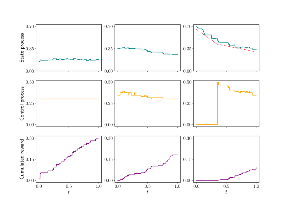
Figure 1: Selected sample realisations of the system for $\epsilon=10^{-1.5}$, starting from ${x=}0.15$ (left), ${x=}{0.35}$ (centre), and ${x=}0.7$ (right).

4.2 Numerical implementation

Adapting (2.4) and (3.4), we normalise the horizon to $1$, and allow the reserve price to vary in $\mathbb{R}$. This allows us to easily set boundary conditions for the equation. When an auction happens with a negative price $x$, the price is set by the competition, which will be a.s. positive. Thus as $x\to-\infty$, the reserve price becomes irrelevant and the value converges to the value of a single auction without reserve price. Conversely, for $\epsilon<1$, as $x\to+\infty$, the probability of $X_{t}^{0,x,\alpha}$ descending below $v$ by time $T$ and generating any revenue decreases due to the noise. Hence, a Neuman boundary condition set to 0 is appropriate at $[0,1)\times\{-\infty,+\infty\}$. In numerical resolution, we will use Neuman boundary conditions equal to 0 on $[0,1)\times{\{-1,3\}}$. Given this domain for the reserve price, we can set the controls on an even mesh in ${{\mathbb{A}}=}[0,{0.5]}$, of fineness $0.01$.

We solve both problems numerically with an explicit finite difference solver, and for simplicity a Riemann sum using the same mesh for the numerical integration part. This formulation is equivalent to a Markov Chain control problem. Let $M_{t}=\{k\Delta_{t}\,;\,k=0,\dots,\lfloor 1/\Delta_{t}\rfloor\}$, $M_{x}={\{-1+k\Delta_{x}\,;\,k=0,\dots,\lfloor 4/\Delta_{x}\rfloor\}}$ be the time and space meshes, with finenesses, $\Delta_{x}=\epsilon^{3/2}/2$, $\Delta_{t}=\Delta_{x}^{2/3}$. Denote $V_{n}(x_{i})$ the output of the solver at time $t_{n}\in\mathcal{{M}}_{t}$ and position $x_{i}\in\mathcal{{M}}_{x}$. For the pure jump problem, we explicitly compute:

$$V_{n}^{\epsilon}(x_{i})=V_{n+1}^{\epsilon}(x_{i})+\frac{\Delta_{t}}{\epsilon}\sup_{a\in\mathbb{A}_{n}}\left(\sum_{x_{j}\in\mathcal{{M}}_{x}}V_{n+1}^{\epsilon}(x_{j})f^{\nu,\epsilon}_{x_{i},a}(x_{j})\Delta_{x}-V_{n+1}^{\epsilon}(x_{i})+r(x_{i},a)\right)\,$$

where $f^{\nu,\epsilon}_{x,a}$ is the transition kernel induced by $b_{1}(x,a,\cdot)$, $b_{2}(x,a,\cdot)$, and $\nu$. For the diffusion, we consider meshes $\mathcal{{M}}_{t}=\{kd_{t}\,;\,k=0,\dots,\lfloor 1/d_{t}\rfloor\}$, $\mathcal{{M}}_{x}={\{-1+kd_{x}\,;\,k=0,\dots,\lfloor 4/d_{x}\rfloor\}}$, with $d_{x}=10^{-2}$, $d_{t}=d_{x}^{2}$ and solve recursively

$$\bar{V}_{n-1}(x_{i})=\bar{V}_{n}(x_{i})+d_{t}\sup_{a\in\mathbb{A}_{n}}\left((\kappa a+(1-\kappa)r_{0}-x)\delta^{u}_{x}\bar{V}_{n}(x_{i})+\frac{1}{2}\sigma^{2}\delta_{xx}\bar{V}_{n}({x_{i}})+r(x_{i},a)\right)$$

where $\delta^{u}_{x}$ and $\delta_{xx}$ are the uplift first order and centred second order finite differences on $\mathcal{{M}}_{x}$ respectively. We took $\mathbb{A}_{n}=\{10^{-2}k;k=0,\dots,{50}\}$ in both cases.

To give some insight into the complexity trade-off, see that, when $\epsilon$ is large, there are relatively few jumps so the time iteration won’t require many steps to get an accurate solution. This scaling is indicated by the $\Delta_{t}/\epsilon$ term. At the same time, the jumps are large so even a coarse mesh in $x$ will be sufficient for the numerical integration to approach the integral. Unfortunately as $\epsilon\to 0$, one must refine both the time mesh, linearly with $1/\epsilon$, and the integration mesh which is paid quadratically due to the non-local nature of the equation. In practice, this makes computations grow at a super-cubic rate with $\epsilon$, which becomes prohibitively expensive quickly. In our example problem, the noise is supported on a bounded interval of size $\sqrt{\epsilon}$, and one thus saves some computation time, but Figure 2 shows the computation cost (pictured with dots) still grows super-quadratically and overcomes the cost of our accurate diffusion mesh (solid horizontal line) even for large $\epsilon$. Even though we computed the diffusive limit to a very high precision, and with an explicit scheme, for $\epsilon$ of order of $10^{-3}$ the CPU time spent on resolution is already $6$ times higher in the pure-jump problem. Note that, in the pure-jump case, if the control were to intervene in a non-linear way we might need to also refine the control mesh with $\epsilon$, further increasing the computational burden.

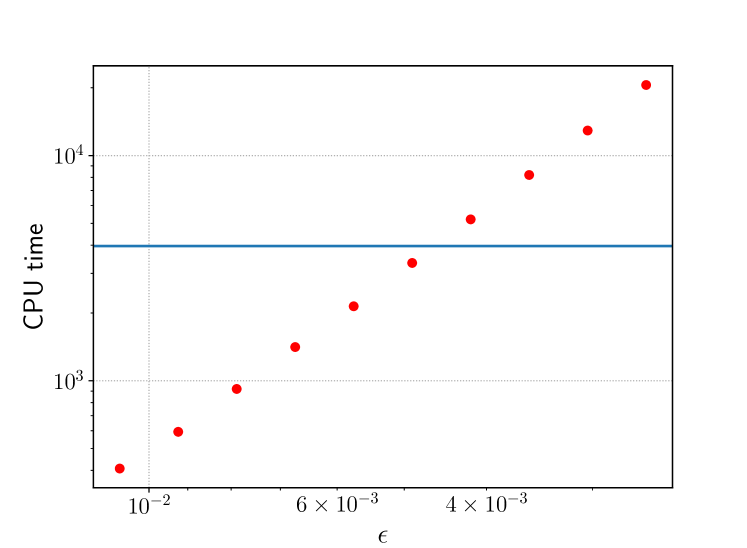
Figure 2: Numerical cost for $V_{\epsilon}$ (log scales).

Beyond gains in computation, Figure 4 verifies that Proposition 3.3 holds with meaningful constants in finite time on this problem. Figure 4 shows that the error is very low even for large values of $\epsilon$, and decreases at the correct rate of $\epsilon^{{1/2}}$. Likewise, Figure 4 shows the rate of Proposition 3.4 also holds even for large $\epsilon$.

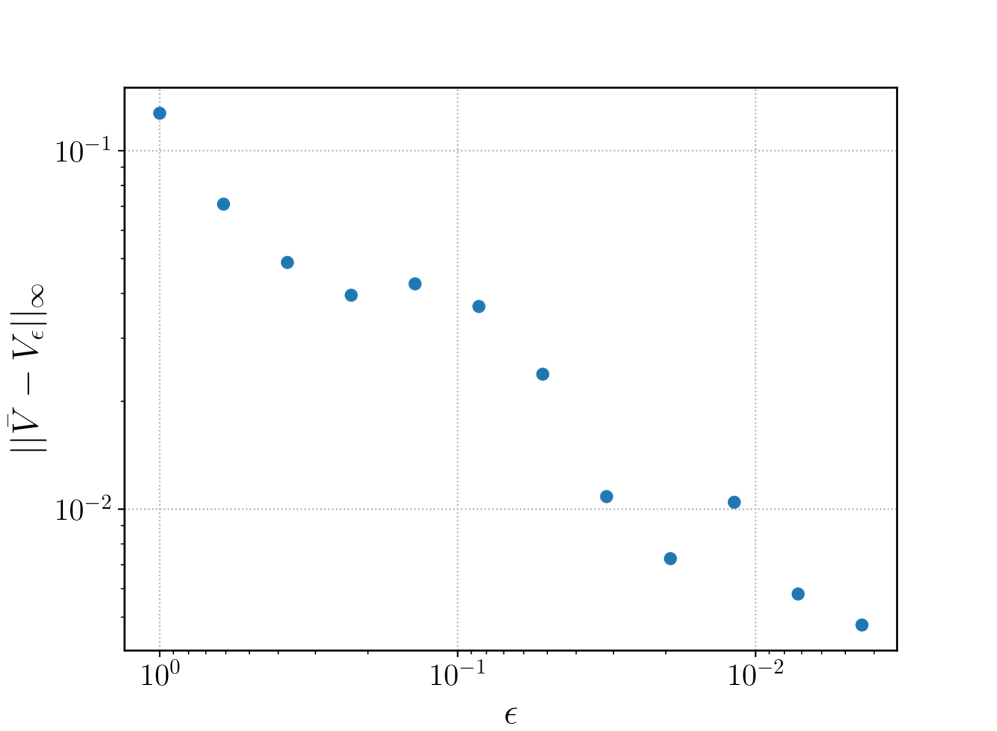
Figure 3: Limit value function error relative to $V_{\epsilon}$, at $t=0$ (log scales).

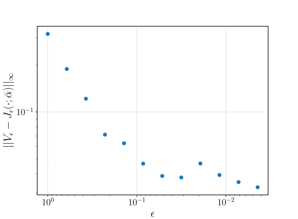
Figure 4: Limit policy error relative to $V_{\epsilon}$, at $t=0$ (log scales).

5 Remark on the diffusive limit of discrete time problems

Instead of considering the diffusive limit of a continuous time pure-jump problem, one could similarly consider a sequence of pure discrete time problems with actions at time $t^{n}_{i}:=iT/n$, $i\leq n$:

$$V_{n}(t,x) :=\sup_{\alpha\in{\mathcal{A}}}\frac{T}{n}\mathbb{E}\left[\sum_{i{=1}}^{n}{\rm 1}_{\{t^{n}_{i}\geq t\}}r(X^{t,x,\alpha}_{t^{n}_{i}-},\alpha_{t^{n}_{i}})\right],$$

with $X^{t,x,\alpha}$ defined by

$$X^{t,x,\alpha}={x+}\sum_{i{=1}}^{n}{\rm 1}_{\{t^{n}_{i}\in(t,\cdot]\}}b(X^{t,x,\alpha}_{t^{n}_{i}-},\alpha_{t^{n}_{i}},\xi_{i}^{n})$$

and in which $(\xi^{n}_{i})_{i\geq 1}$ is i.i.d. following the distribution $\nu$ and ${\mathcal{A}}$ is the collection of ${\mathbb{A}}$-valued processes that are predictable with respect to the ${\mathbb{P}}$-augmented filtration generated by $\sum_{i{=1}}^{n}{\rm 1}_{\{t^{n}_{i}\in[0,\cdot]\}}\xi_{i}^{n}.$

Upon taking $b$ of the form

$$b_{n}=\frac{T}{n}b_{1}+\sqrt{\frac{T}{n}}b_{2},\;\mbox{ with }\mathbb{E}[b_{2}(\cdot,\xi^{n}_{1})]=0,$$

one would obtain the same diffusive limit as in Section 3.3 when letting $n\to\infty$. Namely, the same arguments as in [18, Section 3] combined with Proposition 3.1 and the fact that comparison holds for (3.4) imply that $\lim_{n\to\infty}V_{n}$ is well-defined and is equal to $\bar{V}$.

One can also check that the convergence holds at a speed $n^{-\frac{\beta}{2}}$. Let us sketch the proof. First, the same arguments as in the proof of Theorem 3.3 imply that

$$\delta r_{n}:=\frac{n}{T}{\mathbb{E}\left[\bar{V}(\cdot,\cdot+b_{n}(\cdot,\xi_{i}^{n}))-\bar{V}\right]}-{\mu}\partial_{x}\bar{V}-\frac{1}{2}{\sigma^{2}}\partial_{xx}\bar{V}$$

satisfies

$$\left\lVert\delta r_{n}\right\rVert_{\infty}\leq Cn^{-\frac{\beta}{2}}$$ (5.1)

for some $C>0$ independent on $n$. Thus, by Proposition 3.1

$$0 =\partial_{t}\bar{V}(t,x)\frac{T}{n}+\sup_{a\in{\mathbb{A}}}{\mathbb{E}\left[\bar{V}(t,x+b_{n}(x,a,\xi^{n}_{1}))-\bar{V}(t,x)+\frac{T}{n}(r(x,a)-{\delta r_{n}(x,a)})\right]}$$

so that

$$\bar{V}(t^{n}_{i},x)= \sup_{a\in{\mathbb{A}}}\mathbb{E}\left[\int_{t^{n}_{i}}^{t^{n}_{i+1}}\partial_{t}\bar{V}(t^{n}_{i},x)\mathrm{d}s+\bar{V}(t^{n}_{i},x+b_{n}(x,a,\xi^{n}_{i+1}))+\frac{T}{n}(r(x,a)-{\delta r_{n}(x,a)})\right]$$

$$=\sup_{a\in{\mathbb{A}}}\left(\mathbb{E}\left[\bar{V}(t^{n}_{i+1},x+b_{n}(x,a,\xi^{n}_{i+1}))+\frac{T}{n}r(x,a)\right]\right.$$

$$\leavevmode\nobreak\ \leavevmode\nobreak\ \leavevmode\nobreak\ \leavevmode\nobreak\ \leavevmode\nobreak\ \leavevmode\nobreak\ \leavevmode\nobreak\ \leavevmode\nobreak\ \leavevmode\nobreak\ \leavevmode\nobreak\ +\left.\mathbb{E}\left[\int_{t^{n}_{i}}^{t^{n}_{i+1}}(\partial_{t}\bar{V}(t^{n}_{i},x)-\partial_{t}\bar{V}(s,x+b_{n}(x,a,\xi^{n}_{i+1}))-{\delta r_{n}(x,a)}\mathrm{d}s\right]\right).$$

We then use (3.14) and (5.1) to obtain that

$$\bar{V}(t^{n}_{i},x) =\sup_{a\in{\mathbb{A}}}\mathbb{E}\left[\bar{V}(t^{n}_{i+1},x+b_{n}(x,a,\xi^{n}_{i+1}))+\frac{T}{n}r(x,a)+\int_{t^{n}_{i}}^{t^{n}_{i+1}}\varpi_{n}(s,x,a)\mathrm{d}s\right]$$

in which $|\varpi_{n}|\leq Cn^{-\frac{\beta}{2}}$, for some $C>0$ independent of $n$. It follows that

$$\bar{V}(t^{n}_{i},x)=\sup_{\alpha\in{\mathcal{A}}}\mathbb{E}\left[{\frac{T}{n}\sum_{j=i}^{n}r(X^{t,x,\alpha}_{t^{n}_{j}-},\alpha_{t^{n}_{i}})+\int_{t^{n}_{i}}^{T}\varpi_{n}(s,{X^{t,x,\alpha}_{s}},{\alpha_{s}})\mathrm{d}s}\right],$$

which provides the expected result since $\partial_{t}\bar{V}$ is bounded.

Likewise, the Markovian control defined through (3.23) can be shown to be $n^{-\frac{\beta}{2}}$-optimal for $V_{n}$, see the proof of Proposition 3.4.

6 Conclusion

We studied the diffusion limit of a pure-jump control problem as the jump intensity goes to infinity, upon assuming a correct scaling of the coefficients. Under appropriate conditions, we showed that the second order derivative of the value function associated to the limiting diffusing problem is Hölder continuous and that its Hölder exponent drives the convergence rate. Convergence can even be improved by using a first (or even higher) order correction scheme. This approach is particularly efficient for the numerical approximation of the optimal control associated to a pure jump process with large intensity, as it is the case in auctions associated to online advertising systems.

References

- [1] B. Andrews. Fully nonlinear parabolic equations in two space variables. arXiv preprint math/0402235, 2004.
- [2] G. Barles. Solution de viscosités des équations d’Hamilton Jacobi, volume 17 of Mathématiques et Applications. Springer Verlag, 1994.
- [3] N. Bäuerle. Approximation of optimal reinsurance and dividend payout policies. Mathematical Finance: An International Journal of Mathematics, Statistics and Financial Economics, 14(1):99–113, 2004.
- [4] D. P. Bertsekas and S. E. Shreve. Stochastic Optimal Control. The Discrete-Time Case. Academic Press, New York, 1978.
- [5] A. Blum, V. Kumar, A. Rudra, and F. Wu. Online learning in online auctions. Theoretical Computer Science, 324(2-3):137–146, 2004.
- [6] B. Bouchard. Stochastic targets with mixed diffusion processes and viscosity solutions. Stochastic processes and their applications, 101(2):273–302, 2002.
- [7] B. Bouchard, S. Geiss, and E. Gobet. First time to exit of a continuous Itô process: General moment estimates and -convergence rate for discrete time approximations. Bernoulli, 23(3):1631–1662, 2017.
- [8] B. Bouchard and N. Touzi. Weak dynamic programming principle for viscosity solutions. SIAM Journal on Control and Optimization, 49(3):948–962, 2011.
- [9] P. Brémaud. Point processes and queues: martingale dynamics, Springer series in statistics, 50, Springer, 1981.
- [10] S. Bubeck, N. R. Devanur, Z. Huang, and R. Niazadeh. Multi-scale online learning: Theory and applications to online auctions and pricing. The Journal of Machine Learning Research, 20(1):2248–2284, 2019.
- [11] J. Bulow and P. Klemperer. Auctions versus negotiations. American Economic Review, 86(1):180–94, 1996.
- [12] N. Cesa-Bianchi, C. Gentile, and Y. Mansour. Regret minimization for reserve prices in second-price auctions. IEEE Transactions on Information Theory, 61(1):549–564, 2014.
- [13] H. Chen, D. Yao Fundamentals of Queueing Networks. Stochastic Modeling and Applied Probability, 2001.
- [14] A. Cohen and V. R. Young. Rate of convergence of the probability of ruin in the Cramér–Lundberg model to its diffusion approximation. Insurance: Mathematics and Economics, 93:333–340, 2020.
- [15] M. G. Crandall, H. Ishii, and P.-L. Lions, User’s guide to viscosity solutions of second order partial differential equations. Bull. Amer. Math. Soc. (N.S.), 27(1):1–67, 1992
- [16] L. Croissant, M. Abeille, and C. Calauzenes. Real-time optimisation for online learning in auctions. In Hal Daumé III and Aarti Singh, editors, Proceedings of the 37th International Conference on Machine Learning, volume 119 of Proceedings of Machine Learning Research, pages 2217–2226. PMLR, 13–18 Jul 2020.
- [17] J. Fernandez-Tapia, O. Guéant, and J-M. Lasry. Optimal Real-Time Bidding Strategies. Applied Mathematics Research eXpress, 2017(1):142–183, 09 2016.
- [18] W. H. Fleming and P. E. Souganidis. On the existence of value functions of two-player, zero-sum stochastic differential games. Indiana University Mathematics Journal, 38(2):293–314, 1989.
- [19] J. Jacod and A. Shiryaev. Limit theorems for stochastic processes, volume 288. Springer Science & Business Media, 2013.
- [20] O. A. Ladyzhenskaia, V. Solonnikov, and N. N. Ural’tseva. Linear and quasi-linear equations of parabolic type, volume 23. American Mathematical Soc., 1988.
- [21] G. M. Lieberman. Second order parabolic differential equations. World scientific, 1996.
- [22] R. B. Myerson. Optimal auction design. Mathematics of operations research, 6(1):58–73, 1981.
- [23] M. Ostrovsky and M. Schwarz. Reserve prices in internet advertising auctions: A field experiment. In Proceedings of the 12th ACM Conference on Electronic Commerce, EC ’11, pages 59–60, New York, NY, USA, 2011. Association for Computing Machinery.
- [24] R. Paes Leme, M. Pal, and S. Vassilvitskii. A field guide to personalized reserve prices. In Proceedings of the 25th International Conference on World Wide Web, WWW ’16, pages 1093–1102, Republic and Canton of Geneva, CHE, 2016. International World Wide Web Conferences Steering Committee.
- [25] W. Vickrey. Counterspeculation, auctions, and competitive sealed tenders. The Journal of finance, 16(1):8–37, 1961.