Bootstrap confidence intervals for multiple change points based on moving sum procedures

Abstract

The problem of quantifying uncertainty about the locations of multiple change points by means of confidence intervals is addressed. The asymptotic distribution of the change point estimators obtained as the local maximisers of moving sum statistics is derived, where the limit distributions differ depending on whether the corresponding size of changes is local, i.e. tends to zero as the sample size increases, or fixed. A bootstrap procedure for confidence interval generation is proposed which adapts to the unknown magnitude of changes and guarantees asymptotic validity both for local and fixed changes. Simulation studies show good performance of the proposed bootstrap procedure, and some discussions about how it can be extended to serially dependent errors is provided.

Keywords: Data segmentation, change point estimation, Efron’s Bootstrap, moving sum statistics, scan statistics

1 Introduction

Multiple change point analysis, a.k.a. data segmentation, is an actively researched area with a wide of range of applications in natural and social sciences, medicine, engineering and finance. The canonical data segmentation problem, where the aim is to detect and locate multiple change points in the mean of univariate time series, has received great attention in the past few decades and there exist a variety of methodologies that are computationally fast and achieve consistency in estimating the total number and the locations of multiple change points; see Cho and Kirch, 2021a for an overview of the literature and discussions on how methods proposed for the canonical data segmentation problem offer an important stepping stone for addressing more complex change point problems, such as detecting changes in variance, time series segmentation under parametric models and robust change point analysis.

By contrast, the literature on inference for multiple change points is relatively scarce. Asymptotic (Eichinger and Kirch,, 2018) or approximate (Fang et al.,, 2020) distributions of suitable test statistics have been derived under the null hypothesis of no change point, which enable quantifying uncertainty about the number of change points. A class of multiscale change point segmentation procedures aims at controlling the family-wise error rate (Frick et al.,, 2014) or the false discovery rate (Li et al.,, 2016) of detecting too many change points. There also exist post-selection inference methods which test for a change at estimated change point locations conditional on their estimation procedure, see e.g. Hyun et al., (2021) and Jewell et al., (2019). The Bayesian framework lends itself naturally to change point inference, see Fearnhead, (2006) and Nam et al., (2012).

Another type of uncertainty stems from the localisation of change points. The optimal rate of localisation in change point problems is $O_{P}(1)$ at best (see e.g. Verzelen et al., (2020)), i.e. change point location estimators are not consistent in the usual sense, which makes the problem of inferring uncertainty about change point locations particularly relevant and important. The simultaneous multiscale change point estimator (SMUCE) proposed in Frick et al., (2014) provides a confidence set for all candidate signals from which confidence intervals around the change points can be obtained. Using the inverse relation between confidence intervals and hypothesis tests, Fang et al., (2020) detail how confidence regions can be generated from an approximation of the limit distribution of the test statistic under the null hypothesis. In all of the above, the error distributions are assumed to belong to an exponential family such as Gaussian, or other light-tailed ones. The narrowest significance pursuit (NSP) uses a multi-resolution sup-norm to identify regions containing at least one change point in the mean (Fryzlewicz, 2021a, ) or the median (Fryzlewicz, 2021b, ) at a prescribed confidence level, and allows for heavy-tailed errors.

Meier et al., 2021b outlines the bootstrap construction of confidence intervals around the change points based on the moving sum (MOSUM) procedure proposed in Eichinger and Kirch, (2018). In this paper, we show the theoretical validity of the bootstrap procedure, i.e. that the proposed bootstrap $100(1-\alpha)$%-confidence intervals asymptotically attain the coverage probability of $1-\alpha$ for given $\alpha\in(0,1)$ (see (11) below), and demonstrate its good performance via numerical experiments. Our theoretical contributions build upon the results derived in Antoch et al., (1995) and Antoch and Hušková, (1999) for the case of at most a single change, and accommodate both situations where the changes are local (i.e. tend to zero with the sample size) and when they are fixed while requiring only that the errors have more than two finite moments.

The rest of the paper is organised as follows. Section 2 motivates the use of a bootstrap procedure for confidence interval generation and proposes the bootstrap construction of pointwise and uniform confidence intervals. Section 3 provides results on the asymptotic distributions of change point estimators obtained from the original and the bootstrap data, based on which we establish the validity of bootstrap confidence intervals. In Section 4, we discuss the use of the proposed bootstrap procedure with asymmetric bandwidths and its extension to the case of serially dependent errors. Section 5 shows the good performance of the proposed methodology on simulated datasets in comparison with existing methods and applies it to Hadley Centre central England temperature data, and Section 6 concludes the paper. The implementation of the proposed bootstrap methodology is available in the R package mosum (Meier et al., 2021a, ) as confint method.

2 Bootstrap confidence intervals for change points

In this paper, we consider the following model with multiple change points

$$X_{t} =f_{t}+\varepsilon_{t}=f_{0}+\sum_{j=1}^{q_{n}}d_{j,n}\cdot\mathbb{I}_{\{t>\theta_{j,n}\}}+\varepsilon_{t}=\sum_{j=0}^{q_{n}}\mu_{j,n}\cdot\mathbb{I}_{\{\theta_{j,n}<t\leq\theta_{j+1,n}\}}+\varepsilon_{t},$$ (1)

where $\theta_{j}=\theta_{j,n}$ denote the $q_{n}$ change points (with $\theta_{0}=0$ and $\theta_{q_{n}+1}=n$) at which the mean of $X_{t}$ undergoes changes of (signed) size $d_{j}=d_{j,n}$. We denote by $\delta_{j}=\delta_{j,n}=\min(\theta_{j}-\theta_{j-1},\theta_{j+1}-\theta_{j})$ the minimum distance from $\theta_{j}$ to its neighbouring change points, and by $\Theta=\Theta_{n}=\{\theta_{1},\ldots,\theta_{q_{n}}\}$ the set of change points. Throughout the paper, we focus on the case of i.i.d. errors $\{\varepsilon_{t}\}$ satisfying

$$\mathsf{E}(\varepsilon_{1})=0,\quad 0<\sigma^{2}=\mathsf{var}(\varepsilon_{1})<\infty\quad\text{and}\quad\mathsf{E}(|\varepsilon_{1}|^{\nu})<\infty$$ (2)

for some $\nu>2$, and provide some discussions on the case of dependent errors in Section 4.2.

Under (1), several methods exist that consistently estimate $q_{n}$, the number of change points. On the other hand, the known minimax optimal rate for the estimation of change point locations is $O_{P}(1)$ at best (see e.g. Verzelen et al., (2020)), i.e. the location estimation error does not tend to zero as $n\to\infty$. This makes the task of uncertainty quantification about change point locations by deriving confidence intervals (CI) around $\theta_{j}$, highly important.

In Section 2.1, we motivate the use of a bootstrap procedure for the construction of CIs about change point locations, with a review of its application to the simple case of at-most-one-change (AMOC), i.e. when $q_{n}\leq 1$. Then Section 2.2 describes a procedure based on moving sums for multiple change point detection under (1), and Section 2.3 presents the proposed bootstrap methodology whose validity is established later in Section 3.

2.1 Motivation

In the AMOC setting, classical test statistics such as those based on the CUSUM statistic

$$\mathcal{C}_{k,n}(X)=\sqrt{\frac{k(n-k)}{n}}\left(\bar{X}_{0:k}-\bar{X}_{k:n}\right)\quad\text{with}\quad\bar{X}_{s:e}=\frac{1}{e-s}\sum_{t=s+1}^{e}X_{t},$$

are used to test the null hypothesis $H_{0}:\,q_{n}=0$ (no change point) against $H_{1}:\,q_{n}=1$ (a single change point). When $H_{0}$ is rejected, the CUSUM statistic can directly be used to locate $\theta\equiv\theta_{1}$ by its estimator $\widehat{\theta}=\arg\max_{0<k<n}|\mathcal{C}_{k,n}(X)|$. The asymptotic distribution of $\widehat{\theta}$ depends on unknown quantities, most importantly, on the magnitude of the change. For a local change with $d_{1}=d_{1,n}\to 0$ as $n\to\infty$, the limit is distribution-free (Antoch et al.,, 1995) whereas for a fixed change, the limit depends on the unknown error distribution (Antoch and Hušková,, 1999). Consequently, the asymptotic distribution is of little practical use for constructing a CI about $\theta$ due to the difficulty involved in estimating such quantities.

The bootstrap construction of a CI utilises the difference between the bootstrap estimator, say $\widehat{\theta}^{*}=\arg\max_{0<k<n}|\mathcal{C}_{k,n}(X^{*})|$ maximising the CUSUM statistics computed on a bootstrap sample $\{X_{t}^{*}\}_{t=1}^{n}$, and the original estimator $\widehat{\theta}$, as a proxy for the difference between $\widehat{\theta}$ and the true change point $\theta$. Bootstrap CIs in the AMOC setting have been proposed by Antoch et al., (1995) (accompanied by rigorous proofs for the case of local changes) and Antoch and Hušková, (1999) (their theoretical results cover fixed changes but are given without rigorous proofs). While the asymptotic distributions (and the corresponding proofs) are different in the two regimes determined by the magnitude of $d_{1}$, the same bootstrap procedure can correctly mimic these asymptotic distributions regardless of whether the change is local or fixed, without requiring the knowledge of which regime the problem belongs to or that of the error distribution. As a result, the corresponding bootstrap CI is asymptotically correct in both regimes.

This motivates the use of a bootstrap CI for quantifying uncertainty about the change point location rather than its asymptotic counterpart. An additional testing does not alter the theoretical validity of the bootstrap CI since under $H_{1}$, the test rejects $H_{0}$ with asymptotic power one under weak assumptions even when the nominal level of the test converges slowly to $0$. In such a case, the chance of any false positive also tends to zero asymptotically and, conditional on this asymptotic one-set, the bootstrap CI is either empty (under $H_{0}$) or remains to be asymptotically honest (under $H_{1}$).

2.2 Multiple change point estimation based on moving sums

An obvious difficulty when departing from the AMOC situation is that we do not know the number of change points a priori. For the multiple change point detection problem under (1), Eichinger and Kirch, (2018) propose a moving sum (MOSUM) procedure that makes use of the MOSUM statistic which, for a given bandwidth $G=G_{n}$, is defined as

$$T_{k,n}(G;X)=\sqrt{\frac{G}{2}}\left(\bar{X}_{k-G,k}-\bar{X}_{k,k+G}\right)\quad\text{for}\quad G\leq k\leq n-G.$$ (3)

The statistic $T_{k,n}(G;X)$ takes a large value in modulus around true change points while taking a small value outside their $G$-environments. Therefore, the MOSUM procedure achieves simultaneous detection and localisation of multiple change points by (i) performing a model selection step closely related to change point testing in the AMOC setting, using the asymptotic distribution of $\max_{G\leq k\leq n-G}|T_{k,n}(G;X)|$ under $H_{0}$ to determine ‘significant’ local maxima of the MOSUM statistics, and (ii) identifying the corresponding local maximisers of $|T_{k,n}(G;X)|$ as change point location estimators. Combining the output from the MOSUM procedure applied with a range of bandwidths, it is feasible to perform change point analysis at multiple scales; see Appendix B for further details of the MOSUM procedure and its multiscale extension as proposed by Cho and Kirch, 2021b .

The model selection step in (i) is performed in such a way that the local maximisers in (ii) are asymptotically equivalent to the following oracle estimators:

$$\widetilde{\theta}_{j}=\widetilde{\theta}_{j,n}={\arg\max}_{\theta_{j}-G_{j}<k\leq\theta_{j}+G_{j}}|T_{k,n}(G_{j})|\quad\text{for}\quad j=1,\ldots,q_{n}.$$ (4)

That is, each $\widetilde{\theta}_{j}$ is the local maximiser of the MOSUM statistic in the neighbourhood of $\theta_{j}$ that is determined by a suitable bandwidth $G_{j}$. Here, ‘oracle’ refers to the fact that such estimators are clearly not accessible in practice due to knowing neither the total number nor the locations of the change points. We assume the following on $G_{j},\,j=1,\ldots,q_{n}$:

$$G_{j}=G_{j,n}\to\infty\text{ as }n\to\infty\quad\text{and}\quad 2G_{j}<\delta_{j}.$$ (5)

Eichinger and Kirch, (2018) and Cho and Kirch, 2021b show that MOSUM-based procedures are consistent both in estimating the number of change points as well as their locations and derive the localisation rate (i.e. how close the estimators are to the true change points asymptotically) under mild assumptions on $\{\varepsilon_{t}\}$, see Appendix B. An important step in the proof of such a consistency result is to show that the change point estimators generated by such procedures, say $\widehat{\theta}_{j},\,1\leq j\leq\widehat{q}_{n}$, coincide with the oracle estimators $\widetilde{\theta}_{j},\,1\leq j\leq q_{n}$, on an asymptotic one-set. We formalise this key observation as the following meta-assumption:

Assumption 2.1.

1. For a given $j\in\{1,\ldots,q_{n}\}$, the estimator $\widehat{\theta}_{j}=\widehat{\theta}_{j,n}$ of $\theta_{j}$ satisfies

   $$\mathsf{P}\left(\mathcal{A}_{j}\right)\to 1\text{ as }n\to\infty,\quad\text{where}\quad\mathcal{A}_{j}=\mathcal{A}_{j,n}=\left\{\widehat{\theta}_{j,n}=\widetilde{\theta}_{j,n}\right\}.$$

2. The set of change point estimators $\widehat{\Theta}=\widehat{\Theta}_{n}=\{\widehat{\theta}_{j},\,1\leq j\leq\widehat{q}_{n}:\,\widehat{\theta}_{1}<\ldots<\widehat{\theta}_{\widehat{q}_{n}}\}$ satisfies

   $$\mathsf{P}\left(\mathcal{A}\right)\to 1\text{ as }n\to\infty,\quad\text{where}\quad\mathcal{A}=\mathcal{A}_{n}=\left\{\widehat{q}_{n}=q_{n}\text{ and }\widehat{\theta}_{j,n}=\widetilde{\theta}_{j,n},\,j=1,\ldots,q_{n}\right\}.$$

The equivalence of the oracle estimators and the accessible estimators obtained with a model selection step (as detailed in (9)–(10)), is crucial for the bootstrap CIs introduced in Section 2.3 below, since it allows us to construct bootstrap estimators mimicking the oracle estimators without having to perform any model selection step in the bootstrap world.

2.3 Bootstrap methodology

In this section, we describe the construction of bootstrap CIs for multiple change points, which closely resembles the bootstrap methodology introduced by Antoch et al., (1995) in the AMOC setting.

MOSUM-based change point detection procedures already incorporate some uncertainty quantification for the number of change points and, even their locations, since $|T_{k,n}(G;X)|$ exceeding a critical value indicates that $\{k-G+1,\ldots,k+G\}$ contains a true change point with high probability. However, our aim here is to construct (asymptotically) honest CIs that quantify the uncertainty about the locations of the change points at a prescribed level, with their widths narrower than those given by the bandwidths involved in detecting the corresponding change points.

In what follows, we assume that a set of change point estimators, $\widehat{\Theta}=\{\widehat{\theta}_{j},\,1\leq j\leq\widehat{q}_{n}\}$, is given with $\widehat{q}_{n}$ denoting the estimator of the number of change points, and we adopt the notational convention that $\widehat{\theta}_{0}=0$ and $\widehat{\theta}_{\widehat{q}_{n}+1}=n$. We suppose that each estimator $\widehat{\theta}_{j}$ is detected with a bandwidth $G_{j}$ fulfilling (5), which in turn is used in the construction of bootstrap CIs as described below.

1. Generate a bootstrap sample $\{X_{t}^{*},\,1\leq t\leq n\}$ by randomly drawing $\{X_{t}^{*},\,\widehat{\theta}_{j}<t\leq\widehat{\theta}_{j+1}\}$ with replacement from $\{X_{t},\,\widehat{\theta}_{j}<t\leq\widehat{\theta}_{j+1}\}$ for $j=0,\ldots,\widehat{q}_{n}$.

2. Compute the MOSUM statistics $T_{k,n}(G_{j};X^{*})$ as in (3) with $\{X^{*}_{t}\}$ in place of $\{X_{t}\}$, and locate

   $$\widetilde{\theta}_{j}^{*}={\arg\max}_{\widehat{\theta}_{j}-H_{j}<k\leq\widehat{\theta}_{j}+H_{j}}|T_{k,n}(G_{j};X^{*})|$$ (6)

   for each $j=1,\ldots,q_{n}$, where $H_{j}=\min(G_{j},2\widehat{\delta}_{j}/3)$ with $\widehat{\delta}_{j}=\min(\widehat{\theta}_{j}-\widehat{\theta}_{j-1},\widehat{\theta}_{j+1}-\widehat{\theta}_{j})$.

3. For a given bootstrap sample size $B$, repeat Steps 1–2 $B$ times and record $\widetilde{\theta}_{j}^{*(b)},\,j=1,\ldots,\widehat{q}_{n}$, the local maximisers obtained as in (6), for $b=1,\ldots,B$.

Remark 2.1.

1. In our theoretical analysis, we assume that each $G_{j}$ satisfies (5) in addition to $\widehat{\theta}_{j}-\theta_{j}=o_{P}(\delta_{j})$ (see Assumption 3.1 below) such that $2(\widehat{\theta}_{j}-\widehat{\theta}_{j-1})/3\geq(2/3+o_{P}(1))\delta_{j}\geq(4/3+o_{P}(1))G_{j}$ i.e. $H_{j}=G_{j}$ in (6) with probability converging to one. Consequently, the bootstrap estimator $\widetilde{\theta}_{j}^{*}$ mimics the definition of the oracle estimator $\widetilde{\theta}_{j}$ in (4), with $\widehat{\theta}_{j}$ serving as a change point in the bootstrap sample.

2. In practice, the choice of $G_{j}$ fulfilling (5) is not available and each change point estimator is associated with either a pre-determined bandwidth (as in the case in Eichinger and Kirch, (2018)), or a bandwidth chosen from a range of bandwidths by a multiscale MOSUM procedure (as is the case in Cho and Kirch, 2021b ). Therefore, we cannot guarantee that adjacent estimators, say $\widehat{\theta}_{j-1}$ and $\widehat{\theta}_{j+1}$, are strictly outside the interval $(\widehat{\theta}_{j}-G_{j},\widehat{\theta}_{j}+G_{j}]$. For example, if $\widehat{\theta}_{j-1}$ falls into this interval, two estimators $\widehat{\theta}_{j-1}$ and $\widehat{\theta}_{j}$ compete against each other to be the local maximiser of $|T_{k,n}(G_{j};X^{*})|$ over this interval. When more than $100\,\alpha$% of the bootstrap realisations happen to yield local maxima near $\widehat{\theta}_{j-1}$, the radius of the bootstrap CI is as wide as $G_{j}$ even if the change at $t=\theta_{j}$ (as well as $t=\widehat{\theta}_{j}$ for the bootstrap realisations) is highly pronounced to be detectable. To prevent such events, we propose the slight modification involving $H_{j}$ as in (6) which performs well in practice as shown in Section 5.

At a given level $\alpha\in(0,1)$, a pointwise $100(1-\alpha)\%$ bootstrap CI for each $\theta_{j}$ is constructed as

$$\mathcal{C}^{\text{pw}}_{j}(\alpha) =\left[\widehat{\theta}_{j}-Q_{j}(\alpha),\widehat{\theta}_{j}+Q_{j}(\alpha)\right]\quad\text{with}$$

$$Q_{j}(\alpha) =\inf\left\{c:\,\frac{1}{B}\sum_{b=1}^{B}\mathbb{I}\left(\left|\widetilde{\theta}_{j}^{*(b)}-\widehat{\theta}_{j}\right|\leq c\right)\geq 1-\alpha\right\}.$$ (7)

A uniform bootstrap CI, which provides a guarantee for the simultaneous coverage of $\theta_{j},\,j=1,\ldots,q_{n}$ (as shown later in Section 3), is constructed as follows: Estimating the (signed) size of change as $\widehat{d}_{j}=\bar{X}_{\widehat{\theta}_{j},\widehat{\theta}_{j+1}}-\bar{X}_{\widehat{\theta}_{j-1},\widehat{\theta}_{j}}$, and the (local) variance as

$$\widehat{\sigma}_{j}^{2} =\frac{1}{\widehat{\theta}_{j+1}-\widehat{\theta}_{j-1}-2}\left(\sum_{t=\widehat{\theta}_{j-1}+1}^{\widehat{\theta}_{j}}(X_{t}-\bar{X}_{\widehat{\theta}_{j-1},\widehat{\theta}_{j}})^{2}+\sum_{t=\widehat{\theta}_{j}+1}^{\widehat{\theta}_{j+1}}(X_{t}-\bar{X}_{\widehat{\theta}_{j},\widehat{\theta}_{j+1}})^{2}\right)$$

for $j=1,\ldots,\widehat{q}_{n}$, a uniform $100(1-\alpha)\%$-CI is given by

$$\mathcal{C}^{\text{unif}}_{j}(\alpha) =\left[\widehat{\theta}_{j}-\widehat{d}_{j}^{-2}\widehat{\sigma}_{j}^{2}Q(\alpha),\widehat{\theta}_{j}+\widehat{d}_{j}^{-2}\widehat{\sigma}_{j}^{2}Q(\alpha)\right]\quad\text{with}$$

$$Q(\alpha) =\inf\left\{c:\,\frac{1}{B}\sum_{b=1}^{B}\mathbb{I}\left(\max_{1\leq j\leq\widehat{q}_{n}}\frac{\widehat{d}_{j}^{2}}{\widehat{\sigma}_{j}^{2}}\left|\widetilde{\theta}_{j}^{*(b)}-\widehat{\theta}_{j}\right|\leq c\right)\geq 1-\alpha\right\}.$$ (8)

The quantities $Q_{j}(\alpha)$ (resp. $Q(\alpha)$) are empirical versions of the quantiles of the conditional distribution of $\widetilde{\theta}_{j}^{*}-\widehat{\theta}_{j}$ (as shown in Theorem 3.2 below) obtained by Monte Carlo simulations and converge to the true quantiles as $B\to\infty$, such that the respective bootstrap CIs are asymptotically honest in the sense made precise in (11) below. Unlike the pointwise bootstrap CIs, uniform CIs involve the estimation of the signal-to-noise ratio $d_{j}/\sigma_{j}$ such that $\widetilde{\theta}_{j}^{*}-\widehat{\theta}_{j}$ are treated on an equal footing across $j=1,\ldots,\widehat{q}_{n}$. Lemma A.1 in Appendix A shows that both $\widehat{d}_{j}$ and $\widehat{\sigma}_{j}^{2}$ are consistent and in particular, $\widehat{d}_{j}$ is consistent not only when $d_{j}$ is fixed but also when $d_{j}\to 0$ in the sense that ${\widehat{d}}_{j}/d_{j}\overset{\mathcal{P}}{\to}1$.

3 Theoretical validity of bootstrap confidence intervals

As discussed in Section 2.1, in the AMOC setting, bootstrap CIs have been shown to adapt to whether the (unknown) size of change is local or fixed without requiring the knowledge of the error distribution, which makes their use more practical than the asymptotic CIs. In this section, we show that this is also the case in the presence of multiple change points with the bootstrap procedure introduced in Section 2.3.

In the AMOC setting, the proof of the validity of bootstrap CIs proceeds in two steps: First, the asymptotic distribution of (scaled) difference $\widehat{\theta}-\theta$ is established, and then it is shown that (analogously scaled) $\widehat{\theta}^{*}-\widehat{\theta}$ has the same limit distribution conditional on the observations. When the limit distribution is continuous, quantiles of both differences converge to a true asymptotic quantile such that asymptotic honesty of the bootstrap CIs follows irrespective of the regime determined by the size of the change.

In the multiple change point problem, the estimators $\widehat{\theta}_{j}$ typically involve a model selection step while the construction of bootstrap estimators $\widetilde{\theta}^{*}_{j}$ only mimics the uncertainty stemming from random fluctuations in local maximisation of $|T_{k,n}(G_{j};X^{*})|$ as in (6). Indeed, our bootstrap procedure is designed to mimic the asymptotic distribution of the oracle estimator in (4). Nonetheless, the accessible estimators $\widehat{\theta}_{j}$ asymptotically coincide with the oracle estimators under Assumption 2.1, which allows us to establish the theoretical validity of the proposed bootstrap procedure along the same lines as in the AMOC situation.

For notational ease in the statement of theoretical results, we slightly modify (6) to

$$\widetilde{\theta}_{j}^{*}=\begin{cases}{\arg\max}_{\widehat{\theta}_{j}-G_{j}<k\leq\widehat{\theta}_{j}+G_{j}}|T_{k,n}(G_{j};X^{*})|&\text{for }1\leq j\leq\min(q_{n},\widehat{q}_{n}),\\ 0&\text{for }\widehat{q}_{n}<j\leq q_{n}\end{cases}$$

(see Remark 2.1 (a) for the discussion on asymptotic equivalence between $G_{j}$ and $H_{j}$ appearing in (6)). Also, we define $\widehat{\theta}_{j}=n$ for $\widehat{q}_{n}<j\leq q_{n}$. In doing so, when $\widehat{q}_{n}<q_{n}$, the difference between $\widetilde{\theta}_{j}^{*}$ and $\widehat{\theta}_{j}$ for $\widehat{q}_{n}<j\leq q_{n}$, is made as large as possible. However, this does not influence the asymptotic result due to Assumption 2.1. With these modifications, all the following statements involving the differences $\widetilde{\theta}_{j}^{*}-\widehat{\theta}_{j}$ and $\widehat{\theta}_{j}-\theta_{j}$ are well-defined for any $j=1,\ldots,q_{n}$.

Then under Assumption 2.1, each accessible estimator $\widehat{\theta}_{j}$ coincides with the oracle estimator $\widetilde{\theta}_{j}$ on the asymptotic one-sets $\mathcal{A}_{j}$ and $\mathcal{A}$ (defined in the assumption) such that

$$\sup_{x\in\mathbb{R}}\left|\mathsf{P}\left(\sigma^{-2}d_{j}^{2}|\widehat{\theta}_{j}-\theta_{j}|\leq x\right)-\mathsf{P}\left(\sigma^{-2}d_{j}^{2}|\widetilde{\theta}_{j}-\theta_{j}|\leq x\right)\right| \to 0$$ (9)

and, when $q_{n}=q$ is fixed,

$$\sup_{\mathbf{x}\in\mathbb{R}^{q}}\left|\mathsf{P}\left(\cap_{j=1}^{q}\left\{\sigma^{-2}d_{j}^{2}|\widehat{\theta}_{j}-\theta_{j}|\leq x_{j}\right\}\right)-\mathsf{P}\left(\cap_{j=1}^{q}\left\{\sigma^{-2}d_{j}^{2}|\widetilde{\theta}_{j}-\theta_{j}|\leq x_{j}\right\}\right)\right| \to 0.$$ (10)

In Section 3.1 below, we derive the asymptotic distribution of $\widetilde{\theta}_{j}-\theta_{j}$ and in Section 3.2, we show that the difference $\widetilde{\theta}_{j}^{*}-\widehat{\theta}_{j}$ (conditionally on $X_{1},\ldots,X_{n}$) shares the same limit distribution. Combined with (9)–(10), these results indicate that we can approximate the quantiles of the true difference $\widehat{\theta}_{j}-\theta_{j}$ by those of the bootstrap difference $\widetilde{\theta}_{j}^{*}-\widehat{\theta}_{j}$, which are accessible via Monte Carlo methods. From this, the (asymptotic) validity of the proposed pointwise and uniform CIs follow, i.e.

$$\mathsf{P}\left(\theta_{j}\in\mathcal{C}^{\text{pw}}_{j}(\alpha)\right)\to 1-\alpha\text{ for each $j=1,\ldots,q_{n}$, \ and}$$

$$\mathsf{P}\left(\cap_{j=1}^{q}\left\{\theta_{j}\in\mathcal{C}^{\text{unif}}_{j}(\alpha)\right\}\right)\to 1-\alpha.$$ (11)

3.1 Asymptotic distribution of oracle change point estimators

Theorem 3.1 derives the asymptotic distribution of $\widetilde{\theta}_{j}$ both when the changes are local ($d_{j}=d_{j,n}\to 0$) and when they are fixed. Thanks to Assumption 2.1, the same asymptotic behaviour holds for the accessible change point estimators produced by MOSUM-based procedures.

Theorem 3.1.

Let $\{X_{t}\}_{t=1}^{n}$ satisfy (1)–(2) and $G_{j}$ fulfil (5).

1. If $d_{j}=d_{j,n}\to 0$ and $d_{j}^{2}G_{j}\to\infty$, then it holds as $n\to\infty$,

   $$\sigma^{-2}d_{j}^{2}(\widetilde{\theta}_{j}-\theta_{j})\overset{\mathcal{D}}{\to}\arg\max_{s}\left\{W_{s}-|s|/\sqrt{6}:\,s\in\mathbb{R}\right\}$$

   for $j=1,\ldots,q_{n}$, where $\{W_{s}:\,s\in\mathbb{R}\}$ is a standard Wiener process.

2. If $d_{j}$ is fixed and the errors $\{\varepsilon_{t}\}$ are continuous, then it holds as $n\to\infty$,

   $$\widetilde{\theta}_{j}-\theta_{j}\overset{\mathcal{D}}{\to}\arg\max_{\ell}\left\{-d_{j}\Gamma_{\varepsilon}(\ell)-\ell d_{j}^{2}:\,\ell\in\mathbb{Z}\right\},\quad\text{with}$$

   $$\Gamma_{\varepsilon}(\ell)=\left\{\begin{array}[]{ll}\sum_{t=\ell}^{-1}\varepsilon_{t}^{(1)}-2\sum_{t=\ell}^{-1}\varepsilon_{t}^{(2)}+\sum_{t=\ell}^{-1}\varepsilon_{t}^{(3)}&\text{when }\ell<0,\\ 0&\text{when }\ell=0,\\ \sum_{t=1}^{\ell}\varepsilon_{t}^{(1)}-2\sum_{t=1}^{\ell}\varepsilon_{t}^{(2)}+\sum_{t=1}^{\ell}\varepsilon_{t}^{(3)}&\text{when }\ell>0\end{array}\right.$$

   for $j=1,\ldots,q_{n}$, where $\{\varepsilon_{t}^{(i)},\,t\in\mathbb{Z}\}\overset{\mathcal{D}}{=}\{\varepsilon_{t},\,t\in\mathbb{Z}\}$, $i=1,2,3$, are mutually independent copies of the original error sequence.

3. Suppose that the number of changes is fixed at $q_{n}=q$. For each change point, let the assumptions in (a) or (b) be fulfilled in addition to $4G_{j}<\delta_{j}$. Then it holds as $n\to\infty$,

   $$\sigma^{-2}\left(d_{1}^{2}(\widetilde{\theta}_{j}-\theta_{j}),\ldots,d_{q}^{2}(\widetilde{\theta}_{q}-\theta_{q})\right)\overset{\mathcal{D}}{\to}\left(S_{1},\ldots,S_{q}\right),\quad\text{where}$$

   $$S_{j}=\left\{\begin{array}[]{ll}\arg\max_{s}\{W_{s}^{(j)}-|s|/\sqrt{6}:\,s\in\mathbb{R}\}&\text{when }d_{j}=d_{j,n}\to 0,\\ \sigma^{-2}d_{j}^{2}\arg\max_{\ell}\{-d_{j}\Gamma^{(j)}_{\varepsilon}(\ell)-\ell d_{j}^{2}:\,\ell\in\mathbb{Z}\}&\text{when $d_{j}$ is fixed},\end{array}\right.$$

   with $W_{j}^{(j)}$ (resp. $\Gamma^{(j)}_{\varepsilon}$), $j=1,\ldots,q$, are mutually independent and distributed according to (a) (resp. (b)).

In the case of local changes, the results reported in Theorem 3.1 are closely related to Theorem 3.3 of Eichinger and Kirch, (2018) which also permits time series errors. For the corresponding result in the AMOC situation, see Antoch et al., (1995) (local change) and Antoch and Hušková, (1999) (fixed change). Limiting distributions for multiple change point estimators have also been obtained by Bai and Perron, (1998) in the context of linear models, Yau and Zhao, (2016) for a time series segmentation problem and Kaul and Michailidis, (2021) for the high-dimensional mean change point detection problem.

The additional assumption of continuity of the errors in the case of fixed changes (Theorem 3.1 (b)), is required to avoid ties (a.s.) of the maximum of the limit distribution. If the error distribution is not continuous (e.g. discrete or mixed), those ties may be resolved differently on the RHS of $\overset{\mathcal{D}}{\to}$ than on the LHS, an issue stemming from that the $\arg\max$ is not continuous if the limit does not have a unique, isolated maximum. Therefore, while the underlying process defining the $\arg\max$ on the LHS (denoted by $V_{k,n}$ in the proof given in Appendix A.1) will weakly converge to the process underlying the $\arg\max$ on the RHS (denoted by $\widetilde{V}_{k,n}$ in the proof) even for discrete errors, the $\arg\max$ itself may not because the continuous mapping theorem is not applicable. For the local change considered in (a), the Wiener process with drift on the RHS does not suffer from this issue and thus the continuity of the errors is not required. Ferger, (2004) provide additional insights into the theoretical behaviour of the $\arg\max$ if ties occur. In practice, we may either ignore the ties or report their occurrence explicitly.

As in the AMOC situation, the asymptotic behaviour of the oracle estimator $\widetilde{\theta}_{j}$ (and by Assumption 2.1, the accessible estimator $\widehat{\theta}_{j}$) depends on the regime determined by the magnitude of the change and, in the fixed change case, on the unknown error distribution. Consequently, the limit distribution itself is not suitable for CI generation. Section 3.2 shows that for the bootstrap estimators $\widetilde{\theta}_{j}^{*}$, we have $\widetilde{\theta}_{j}^{*}-\widehat{\theta}_{j}$ (conditional on the data) mimic the distribution of $\widetilde{\theta}_{j}-\theta_{j}$, and thus the bootstrap procedure produces asymptotically honest bootstrap CIs under Assumption 2.1.

3.2 Asymptotic distribution of bootstrap change point estimators

Since the bootstrap procedure is based on the change point estimators $\widehat{\Theta}=\{\widehat{\theta}_{j},\,1\leq j\leq\widehat{q}_{n}\}$, we require the estimators to be sufficiently precise in the following sense:

Assumption 3.1.

For given $j\in\{1,\ldots,q_{n}\}$, we have

$$\widehat{\theta}_{i}-\theta_{i}=o_{P}(\delta_{i})\quad\text{for}\quad i\in\{j-1,j,j+1\},\qquad\text{and}$$

$$d_{i}^{2}(\widehat{\theta}_{i}-\theta_{i})=o_{P}(d_{j}^{2}|\theta_{j}-\theta_{i}|)\quad\text{for}\quad i\in\{j-1,j+1\}.$$

As in the case of Assumption 2.1, MOSUM-based change point detection procedures achieve consistency in multiple change point estimation and thus produce estimators that fulfil Assumption 3.1; we refer to Appendix B for detailed discussions.

Theorem 3.2.

Denote $\mathsf{P}^{*}(\cdot)=\mathsf{P}(\cdot|X_{1},\ldots,X_{n})$. Let (1)–(2) and Assumption 3.1 hold (for a given $j$ in (a) and (b), and for all $j$ in (c)), and $G_{j}$ fulfil (5).

1. If $d_{j}=d_{j,n}\to 0$ and $d_{j}^{2}G_{j}\to\infty$, then the following limit distribution holds for all $x\in\mathbb{R}$ as $n\to\infty$,

   $$\mathsf{P}^{*}\left(\sigma^{-2}d_{j}^{2}(\widetilde{\theta}^{*}_{j}-\widehat{\theta}_{j})\leq x\right)\overset{\mathcal{P}}{\to}\mathsf{P}\left(\arg\max_{s\in\mathbb{R}}\left\{W_{s}-|s|/\sqrt{6}\right\}\leq x\right)$$

   for each $j=1,\ldots,q_{n}$, where $\{W_{s}\}$ is as in Theorem 3.1 (a).

2. If $d_{j}$ is fixed and the errors $\{\varepsilon_{j}\}$ are continuous, then the following limit distribution holds for all $x\in\mathbb{R}$ as $n\to\infty$,

   $$\mathsf{P}^{*}\left(\widetilde{\theta}^{*}_{j}-\widehat{\theta}_{j}\leq x\right)\overset{\mathcal{P}}{\to}\mathsf{P}\left(\arg\max_{\ell\in\mathbb{Z}}\left\{-d_{j}\Gamma_{\varepsilon}(\ell)-\ell d_{j}^{2}\right\}\leq x\right)$$

   for $j=1,\ldots,q_{n}$, where $\{\Gamma_{\varepsilon}(\ell)\}$ is as in Theorem 3.1 (b).

3. Suppose that the number of changes is fixed at $q_{n}=q$. For each change point, let the assumptions in (a) or (b) be fulfilled in addition to $4G_{j}<\delta_{j}$. Then, the following limit distribution holds for all $\mathbf{x}=(x_{1},\ldots,x_{q})^{\top}\in\mathbb{R}^{q}$ as $n\to\infty$,

   $$\mathsf{P}^{*}\left(\sigma^{-2}d_{1}^{2}(\widetilde{\theta}_{1}^{*}-\widehat{\theta}_{1})\leq x_{1},\ldots,\sigma^{-2}d_{q}^{2}(\widetilde{\theta}_{q}^{*}-\widehat{\theta}_{q})\leq x_{q}\right)\overset{\mathcal{P}}{\to}\mathsf{P}\left(S_{1}\leq x_{1},\ldots,S_{q}\leq x_{q}\right),\text{ where}$$

   $$S_{j}=\left\{\begin{array}[]{ll}\arg\max_{s}\{W_{s}^{(j)}-|s|/\sqrt{6}:\,s\in\mathbb{R}\}&\text{when }d_{j}=d_{j,n}\to 0,\\ \sigma^{-2}d_{j}^{2}\arg\max_{\ell}\{-d_{j}\Gamma^{(j)}_{\varepsilon}(\ell)-\ell d_{j}^{2}:\,\ell\in\mathbb{Z}\}&\text{when $d_{j}$ is fixed},\end{array}\right.$$

   with $\{W_{j}^{(j)}\}$ (resp. $\{\Gamma^{(j)}_{\varepsilon}\}$), $j=1,\ldots,q$, are mutually independent and distributed according to (a) (resp. (b)).

To the best of our knowledge, the literature on bootstrap CIs for change points considers only the case of local changes with a distribution-free limit; an exception is Antoch and Hušková, (1999) where their Theorem 7.1 (given without an explicit proof) is on the fixed change case in the AMOC setting.

3.3 Consistency of the bootstrap procedure

Recall that by Assumption 2.1, the accessible estimators $\widehat{\theta}_{j}$ coincide with the oracle ones $\widetilde{\theta}_{j}$ on asymptotic one-sets such that (9)–(10) follow. Then, Theorems 3.1 and 3.2 establish that for each $j=1,\ldots,q_{n}$,

$$\sup_{x\in\mathbb{R}}\left|\mathsf{P}^{*}\left(\sigma^{-2}d_{j}^{2}|\widetilde{\theta}_{j}^{*}-\widehat{\theta}_{j}|\leq x\right)-\mathsf{P}\left(\sigma^{-2}d_{j}^{2}|\widehat{\theta}_{j}-\theta_{j}|\leq x\right)\right|\overset{\mathcal{P}}{\to}0$$

and, when $q_{n}=q$ is fixed,

$$\sup_{\mathbf{x}\in\mathbb{R}^{q}}\left|\mathsf{P}^{*}\left(\cap_{j=1}^{q}\left\{\sigma^{-2}d_{j}^{2}|\widetilde{\theta}_{j}^{*}-\widehat{\theta}_{j}|\leq x_{j}\right\}\right)-\mathsf{P}^{*}\left(\cap_{j=1}^{q}\left\{\sigma^{-2}d_{j}^{2}|\widehat{\theta}_{j}-\theta_{j}|\leq x_{j}\right\}\right)\right|\overset{\mathcal{P}}{\to}0.$$

Together with that $\widehat{d}_{j}/d_{j}\overset{\mathcal{P}}{\to}1$ (Lemma A.1) and Assumption 2.1, the validity of the bootstrap CIs proposed in (7)–(8) follows in the sense of (11). In particular, the bootstrap CIs are asymptotically honest whether the changes are local or fixed, although their construction does not require the knowledge of the regime determined by the magnitude of the changes or the error distribution. The additional model selection step involved in the estimators $\widehat{\theta}_{j}$ does not alter the theoretical validity of the bootstrap CIs by Assumption 2.1.

The simulation studies reported in Section 5 show that the coverage of the bootstrap CI constructed with the oracle estimators $\widetilde{\theta}_{j}$ is generally right on target as expected from the above asymptotic theory. While asymptotically equivalent, bootstrap CIs constructed with the estimators $\widehat{\theta}_{j}$ involving an additional model selection step, have somewhat more conservative coverage in finite samples. Heuristically, this is not surprising as in the latter case, the empirical coverage is computed conditioning on the success of the model selection step, and changes underlying those realisations belonging to the conditioning set tend to be more pronounced.

4 Extensions

4.1 Asymmetric bandwidths

The MOSUM statistic defined in (3) is readily extended to accommodate the use of asymmetric bandwidths $\mathbf{G}=(G_{\ell},G_{r})$, as

$$T_{k,n}(\mathbf{G};X)=\sqrt{\frac{G_{\ell}G_{r}}{G_{\ell}+G_{r}}}\left(\bar{X}_{k-G_{\ell},k}-\bar{X}_{k,k+G_{r}}\right),\quad k=G_{\ell},\ldots,n-G_{r}.$$

In practice, provided that the asymmetric bandwidth is not too unbalanced, its use can improve small sample performance of the MOSUM procedure, see Figure 6 of Meier et al., 2021b for an illustration. Their Theorem 1 extends the asymptotic null distribution of the MOSUM test statistic to the asymmetric case and similarly, we can extend Theorem 3.1 and derive the asymptotic distribution of the corresponding (oracle) change point estimators obtained as in (4), i.e. with the bandwidth $\mathbf{G}_{j}=(G_{j,\ell},G_{j,r})$,

$$\widetilde{\theta}_{j}={\arg\max}_{\theta_{j}-G_{j,\ell}<k\leq\theta_{j}+G_{j,r}}|T_{k,n}(\mathbf{G}_{j};X)|.$$

Analogously, we obtain the bootstrap estimators as

$$\widetilde{\theta}_{j}^{*}={\arg\max}_{\widehat{\theta}_{j}-H_{j,\ell}<k\leq\widehat{\theta}_{j}+H_{j,r}}|T_{k,n}(\mathbf{G}_{j};X^{*})|,$$

where $H_{j,\ell}=\min\{G_{j,\ell},2(\widehat{\theta}_{j}-\widehat{\theta}_{j-1})/3\}$ and $H_{j,r}=\min\{G_{j,r},2(\widehat{\theta}_{j+1}-\widehat{\theta}_{j})/3\}$, similarly as in Section 2.3. Then analogously, we approximate the distribution of $\widetilde{\theta}_{j}-\theta_{j}$ with that of $\widetilde{\theta}_{j}^{*}-\widehat{\theta}_{j}$, using the symmetric construction of the CIs by means of $Q_{j}(\alpha)$ and $Q(\alpha)$ defined as in (7) and (8).

4.2 Dependent errors

In practice, it is more natural to allow for serial dependence in $\{\varepsilon_{t}\}$. In the context of testing for a mean in the AMOC setting, different time series bootstrap methods have successfully been applied such as block permutation Kirch, (2007), block bootstrap Sharipov et al., (2016) or frequency domain-based Kirch and Politis, (2011) methods, and subsampling has been studied by Betken and Wendler, (2018) in the context of mean change point analysis in long-range dependent time series; there also exist bootstrap-based testing procedures for more complex change point problems, see e.g. Bücher and Kojadinovic, (2016) and Emura et al., (2021).

For the multiple change point detection problem in (1), compared to the i.i.d. setting, there are fewer methods that guarantee consistent change point estimation when serial correlations are permitted in $\{\varepsilon_{t}\}$, such as those proposed in Tecuapetla-Gómez and Munk, (2017), Dette et al., (2020), Romano et al., (2021) and Cho and Fryzlewicz, (2020). The single-scale MOSUM procedure studied in Eichinger and Kirch, (2018) and the multiscale MOSUM procedure combined with the localised pruning proposed in Cho and Kirch, 2021b , have been shown to yield consistent estimators for heavy-tailed and/or serially correlated $\{\varepsilon_{t}\}$, see Appendix B.

A natural question is whether we can automatically adapt to the regime determined by the magnitude of changes using time series bootstrap methods. While for local changes, most time series bootstrap methods are expected to yield consistent results, this is no longer the case for the fixed change situation where a standard block bootstrap procedure will not work off the shelf. In this section, we aim at explaining where the main difficulties lie in the construction of bootstrap CIs for change point locations in time series settings.

For local changes, the limit distribution follows from a central limit theorem such that time series bootstrap methods are expected to work well. Indeed, in the AMOC setting with a local change, Hušková and Kirch, (2008, 2010) propose to use a block bootstrap and show its asymptotic validity. More precisely, in place of Step 1 of the bootstrap procedure proposed in Section 2.3, one draws blocks of length $K$ (with $K=K_{n}\to\infty$ at an appropriate rate) from the estimated residuals $\widehat{\varepsilon}_{t}=X_{t}-\widehat{f}_{t}$ to form a bootstrap sample $\{X_{t}^{*}\}$, where $\widehat{f}_{t}$ denotes the piecewise constant signal that takes into account the possible presence of the single change point. With some additional technicality, the results in Hušková and Kirch, (2010) can be extended to show the consistency of thus-constructed bootstrap CIs for multiple local changes under the problem (1) considered here. Other time series bootstrap procedures such as a stationary bootstrap, dependent wild bootstrap or even frequency domain methods are similarly conjectured to achieve consistency.

However, the case of fixed changes needs to be handled with more care in the presence of serial dependence, since the limit distribution is no longer based on a central limit theorem such that one cannot generally expect a bootstrap procedure to work well. The success of the bootstrap method in the i.i.d. case is due to that $\widetilde{\theta}_{j}-\theta_{j}=O_{P}(1)$ (see (12) in the proof of Theorem 3.1 in Appendix A.1), i.e. the asymptotic distribution of $\widetilde{\theta}_{j}$ effectively depends on a sequence of finitely many errors. The joint distribution of this sequence must be mimicked correctly for the construction of the CIs, and the i.i.d. bootstrap described in Section 2.3 correctly approximates the joint distribution of finitely many independent errors asymptotically thanks to the consistency of the empirical distribution function, see (23) in the proof of Theorem 3.2.

In the time series case, for the validity of bootstrap CIs, a bootstrap procedure is required to correctly mimic the joint dependence structure of the three relevant finite stretches appearing in (23) (see also (14) to see where the three stretches come from). While the three stretches are (asymptotically) independent under appropriate assumptions, for correct approximation of the joint distribution, each of these stretches needs to be covered by a single block; if a bootstrap procedure does not fulfil this requirement and two blocks are involved in covering one of those stretches (involvement of more than two blocks is not possible asymptotically as the block length diverges while the length of each stretch is finite), then those two blocks are (conditionally) independent unlike the original series and (23) does not hold.

One possible approach to fulfil this requirement is to center bootstrapped blocks from the residuals $\{\widehat{\varepsilon}_{t}\}$ at the estimator $\widehat{\theta}_{j}$ as well as $\widehat{\theta}_{j}\pm G_{j}$ for individual $j=1,\ldots,\widehat{q}_{n}$. Since in effect, the asymptotic distribution such as that reported in Theorem 3.1 (b) depends on finitely many observations around $\widehat{\theta}_{j}$ and $\widehat{\theta}_{j}\pm G_{j}$ only, this bootstrap procedure essentially amounts to subsampling where only one block for each of the three stretches (which can be considered as a subsample) is involved in determining the distribution of $\widetilde{\theta}_{j}^{*}$ for individual change points. Alternatively, for small enough bandwidths $G_{j}$ (asymptotically, since smaller bandwidths are permitted as more moments exist for $\{\varepsilon_{t}\}$), one can use a block length $K$ diverging faster than $G_{j}$ such that a single block centered at $\widehat{\theta}_{j}$ covers all three stretches simultaneously. A similar idea is explored in Ng et al., (2021) who also suggest to apply subsampling locally at the estimated change point locations.

To summarise, while many time series resampling procedures are expected to return valid bootstrap CIs for local changes, the same will typically not be the case for fixed changes without a carefully designed subsampling method that takes into account the specific structure of the asymptotic distribution involved, and their good practical performance will require longer stretches of stationarity between adjacent change points.

5 Numerical studies

In this section, we investigate the practical performance of the bootstrap CIs on simulated datasets. We consider both the bootstrap CIs constructed with the oracle estimators $\widetilde{\theta}_{j}$ as in (4) (which are inaccessible in practice), and those based on the change point estimators $\widehat{\theta}_{j}$ which are obtained after a model selection step. In the former case, we expect the bootstrap CIs to closely attain the given confidence level since the bootstrap actually mimics the distribution of $\widetilde{\theta}_{j}$. While the model selection step employed for $\widehat{\theta}_{j}$ is asymptotically negligible, simulation results suggest that it leads to somewhat more conservative CIs for the latter case in small samples.

5.1 Set-up

We consider the test signals blocks, fms, mix, teeth10 and stairs10 first introduced in Fryzlewicz, (2014), see Figure 6 in Appendix which plots realisations from the five test signals with Gaussian errors. We introduce an additional scaling factor $\vartheta$ and modify the test signals as follows: Denoting the mean of the original test signal by $f^{\circ}_{t}=f^{\circ}_{0}+\sum_{j=1}^{q_{n}}d_{j}^{\circ}\mathbb{I}_{\{t>\theta_{j}^{\circ}\}}$, with the locations of the change points therein by $\theta^{\circ}_{j}$ and the (signed) size of change by $d^{\circ}_{j}$ for $j=1,\ldots,q_{n}$, we consider the scaled signals $f_{t}=f^{\circ}_{0}+\sum_{j=1}^{q_{n}}d_{j}\mathbb{I}_{\{t>\theta_{j}\}}$ with $d_{j}=d^{\circ}_{j}/\vartheta$ and the change points $\theta_{j},\,j=1,\ldots,q_{n}$ satisfying $\theta_{j+1}-\theta_{j}=\vartheta^{2}(\theta^{\circ}_{j+1}-\theta^{\circ}_{j})$. In doing so, we keep the detectability of each change point determined by $d_{j}^{2}\delta_{j}$ constant across the scaling factor $\vartheta$, while exploring the two different regimes – the local change where $d_{j}=d_{j,n}\to 0$ and the fixed change with constant $d_{j}$ – by varying $\vartheta\in\{1,2,4\}$. In what follows, we only report the results from $\vartheta\in\{1,4\}$ (with $\vartheta=1$ corresponding to the fixed change regime and $\vartheta=4$ to the local one) for brevity. Also, we only provide the results for mix and teeth10 test signals when $\{\varepsilon_{t}\}$ follow Gaussian distributions in the main text, and the rest of the simulation results, including when the errors follow $t_{5}$ distributions, are given in the supplement (see Appendix C); we observe little difference is observed in the results obtained with either Gaussian or $t_{5}$-distributed errors.

All results given below and in Appendix C are based on $2000$ realisations for each simulation setting (with the exception of Section 5.2.3 where $1000$ realisations were generated), and we set $B=1000$ for bootstrap sample generation. We consider $1-\alpha\in\{0.8,0.9,0.95\}$ for the confidence levels.

5.2 Results

5.2.1 Bootstrap CIs constructed with the oracle estimators in (4)

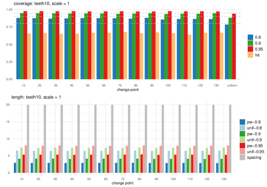
(a) $\vartheta=1$.

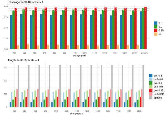
(b) $\vartheta=4$.

Figure 1: teeth10: Bootstrap CIs constructed with the oracle estimators in (4). Top panel (of each sub-figure): coverage of pointwise bootstrap CIs for each $\theta_{j}$ (their locations given as the $x$-axis labels) and that of the uniform ones. Horizontal lines indicate $1-\alpha\in\{0.8,0.9,0.95\}$. We also report the proportion of the event where $\widehat{\theta}_{j}=\theta_{j}$ exactly (‘hit’). Bottom: lengths of pointwise and uniform bootstrap CIs at $1-\alpha\in\{0.8,0.9,0.95\}$. The grey columns ‘spacing’ reports twice the minimum distance to adjacent change points $2\delta_{j}$, for each $\theta_{j},\,j=1,\ldots,q_{n}$.

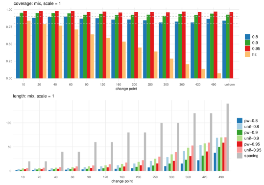
(a) $\vartheta=1$.

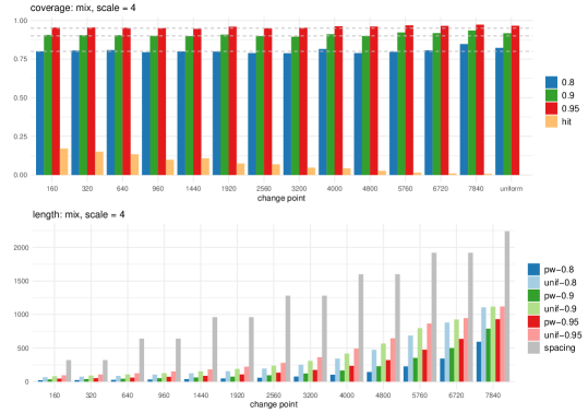
(b) $\vartheta=4$.

Figure 2: mix: Bootstrap CIs constructed with the oracle estimators in (4). See Figure 1 for detailed descriptions.

We first investigate the coverage and the length of bootstrap CIs generated with the estimators $\widetilde{\theta}_{j}$ defined in (4) with $G_{j}=\delta_{j}/2$ for all $j=1,\ldots,q_{n}$, which do not involve any model selection step that amounts to testing whether there indeed exist change points in their vicinity or not. When possibly multiple change points are present, the oracle estimators $\widetilde{\theta}_{j}$ are accessible only in simulations. In contrast, an analogue of $\widetilde{\theta}_{j}$ is accessible in the AMOC setting, and Hušková and Kirch, (2008) take a similar approach in their simulation studies. For given $j$, the coverage of pointwise CIs is calculated as the proportion of simulation realisations where $\mathcal{C}_{j}^{\text{pw}}$ contains $\theta_{j}$. For the uniform CIs, it is calculated as the proportion of the realisations where the uniform bootstrap CIs $\mathcal{C}_{j}^{\text{unif}}$ contain the corresponding $\theta_{j}$ simultaneously for all $j=1,\ldots,q_{n}$. The lengths of CIs reported are obtained by averaging the respective CIs over the $2000$ realisations.

Figures 1–2 report the coverage and the lengths of bootstrap CIs for teeth10 and mix test signals with $\vartheta\in\{1,4\}$, when $\{\varepsilon_{t}\}$ are generated from Gaussian distributions. The reported coverage is close to the nominal level throughout the test signals and $\vartheta$, while the lengths of CIs are not trivial, i.e. the CIs are considerably shorter than the distance to neighbouring change points. We observe that the coverage gets closer to the nominal level with increasing $\vartheta$, i.e. as the size of changes corresponds to the local change regime, which agrees with that the hit rate is considerably lower when $\vartheta=4$ compared to when $\vartheta=1$. Since the bootstrap CIs are for discrete quantities, they are expected not to achieve the confidence level exactly but to be on the conservative side, particularly with smaller $\vartheta$ which corresponds to the fixed change regime (see Theorem 3.1 (b) where the limit distribution of $\widetilde{\theta}_{j}$ is discrete, in contrast to that of the local change regime as in (a)). Between $\vartheta\in\{1,4\}$, the absolute lengths of the CIs are naturally greater when $\vartheta=4$, but their ratio to the corresponding minimum spacing $\delta_{j}$ remains approximately constant across $\vartheta$.

5.2.2 Bootstrap CIs constructed with model selection

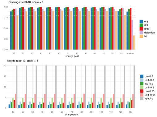
(a) $\vartheta=1$.

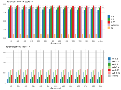
(b) $\vartheta=4$.

Figure 3: teeth10: Bootstrap CIs constructed with model selection. Top panel (of each sub-figure): coverage of pointwise bootstrap CIs for each $\theta_{j}$ (their locations given as the $x$-axis labels) and that of the uniform ones. Horizontal lines indicate $1-\alpha\in\{0.8,0.9,0.95\}$. We also report the proportion of the event where $\widehat{\theta}_{j}=\theta_{j}$ exactly (‘hit’), and that where we do detect the corresponding change points (‘detection’). Bottom: lengths of pointwise and uniform bootstrap CIs at $1-\alpha\in\{0.8,0.9,0.95\}$. The grey columns ‘spacing’ reports twice the minimum distance to adjacent change points $2\delta_{j}$, for each $\theta_{j},\,j=1,\ldots,q_{n}$.

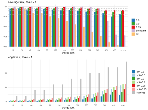
(a) $\vartheta=1$.

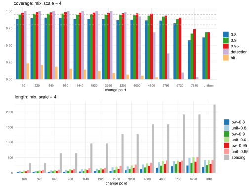
(b) $\vartheta=4$.

Figure 4: mix: Bootstrap CIs constructed with model selection. See Figure 3 for detailed descriptions.

We examine the performance of bootstrap CIs when applied with the change point estimators from the two-stage change point detection procedure proposed in Cho and Kirch, 2021b : Termed MoLP, it first generates candidate change point estimators using the MOSUM procedure with a range of bandwidths (which includes asymmetric bandwidths discussed in Section 4.1), and then prunes down the set of candidates to obtain the final estimators via the localised pruning methodology proposed therein, see Appendix B for further details. The implementation of this two-stage procedure is readily available as the function multiscale.localPrune in the R package mosum (Meier et al., 2021a, ), and we apply it with all the tuning parameters chosen as recommended by default; the set of bandwidths is also obtained according to the automatic bandwidth generation implemented therein with the minimum bandwidth set at $10\vartheta$. Here, $G_{j}$ denotes the bandwidth at which the change point estimator $\widehat{\theta}_{j}$ is detected which is chosen in a data-driven way and therefore often differs from $\delta_{j}/2$. For the test signals teeth10 and stairs10 with $\vartheta=1$, the set of bandwidths excludes the bandwidth $G_{j}=5$ used in Section 5.2.1, as the minimum bandwidth coincides with the minimum spacing $\delta_{j}=10$ of those signals. Even in this adverse situation where the condition $2G_{j}<\delta_{j}$ required for Theorem 3.2 is violated, the proposed methodology works well. Some preliminary numerical results indicate that the issue discussed in Remark 2.1 occurs in this situation, if the bootstrap estimator is calculated over the $G_{j}$-environment around each of the original change point estimators instead of the modified one used in (6).

Unlike in Section 5.2.1, the set of estimators $\widehat{\Theta}$ returned by MoLP may not contain the estimators for all $\theta_{j},\,j=1,\ldots,q_{n}$, in practice. Therefore, we match each change point $\theta_{j}$ with an estimator $\widehat{\theta}\in\widehat{\Theta}$ as follows: If $\widehat{\Theta}\cap\mathcal{I}_{j}\neq\emptyset$ with $\mathcal{I}_{j}=\{\lfloor(\theta_{j-1}+\theta_{j})/2\rfloor+1,\ldots,\lfloor(\theta_{j}+\theta_{j+1})/2\rfloor\}$, we regard that $\theta_{j}$ has been detected, and set an indicator $Z_{j}=1$; otherwise, we set $Z_{j}=0$. If there are multiple estimators falling into the set $\mathcal{I}_{j}$, we set the one closest to $\theta_{j}$ as its estimator $\widehat{\theta}_{j}$. Then, the coverage of the pointwise CIs is calculated as the proportion of realisations where $\mathcal{C}^{\text{pw}}_{j}$ contains $\theta_{j}$ conditional on $Z_{j}=1$, for individual $j=1,\ldots,q_{n}$. The coverage of the uniform CIs is calculated as that of $\mathcal{C}^{\text{unif}}_{j}$ containing $\theta_{j}$, conditional on $|\widehat{\Theta}|=q_{n}$ and $Z_{j}=1$ simultaneously for all $j=1,\ldots,q_{n}$; the lengths of the CIs are also calculated by taking average conditional on the detection of the corresponding change points. Figures 3–4 plot the results from the teeth10 and mix test signals when $\vartheta\in\{1,4\}$.

Table 1: Average coverage of the bootstrap $90\%$-CIs constructed with the oracle estimators and the estimators obtained from MoLP. Under each ‘$\theta_{j}$’, we report the coverage of the corresponding pointwise CI and under ‘uniform’, that of the uniform CI as described in the main text.

We also report the proportion of realisations where individual change points are detected (by MoLP) and where all change points are correctly detected (see the rows headed ‘detection’). test signal $\vartheta$ estimator $\theta_{1}$ $\theta_{2}$ $\theta_{3}$ $\theta_{4}$ $\theta_{5}$ $\theta_{6}$ $\theta_{7}$ $\theta_{8}$ $\theta_{9}$ $\theta_{10}$ $\theta_{11}$ $\theta_{12}$ $\theta_{13}$ uniform mix 1 oracle 0.956 0.948 0.95 0.946 0.926 0.938 0.922 0.926 0.928 0.908 0.934 0.922 0.942 0.927 MoLP 0.964 0.981 0.972 0.971 0.974 0.969 0.965 0.964 0.953 0.931 0.93 0.894 0.857 0.888 detection 0.999 0.999 1 1 1 1 1 1 1 0.994 0.938 0.635 0.3 0.279 4 oracle 0.906 0.904 0.905 0.9 0.898 0.908 0.898 0.895 0.911 0.9 0.922 0.918 0.935 0.917 MoLP 0.948 0.959 0.96 0.961 0.945 0.952 0.946 0.942 0.938 0.933 0.919 0.883 0.672 0.692 detection 1 1 1 1 0.999 0.999 0.998 0.982 0.921 0.692 0.376 0.098 0.031 0.0065 teeth10 1 oracle 0.948 0.946 0.944 0.941 0.942 0.942 0.936 0.94 0.946 0.935 0.939 0.938 0.946 0.882 MoLP 0.933 0.993 0.994 0.992 0.996 0.995 0.992 0.991 0.991 0.993 0.994 0.991 0.946 0.954 detection 0.962 0.946 0.948 0.952 0.952 0.951 0.951 0.954 0.953 0.951 0.948 0.952 0.964 0.7 4 oracle 0.904 0.928 0.916 0.927 0.916 0.916 0.926 0.923 0.919 0.92 0.918 0.922 0.908 0.964 MoLP 0.923 0.933 0.928 0.929 0.926 0.912 0.929 0.924 0.925 0.919 0.914 0.92 0.921 0.91 detection 0.918 0.902 0.908 0.913 0.921 0.926 0.92 0.91 0.908 0.901 0.916 0.915 0.921 0.526

For those change points that are well-detected, the coverage observed here tends to be slightly more conservative compared to that reported in Section 5.2.1, which is attributed to the additional testing and conditioning, see Table 1 for an overview of the comparison. On the other hand, for change points which are difficult to detect (i.e. the test statistics in their vicinity do not exceed the theoretically motivated threshold due to the corresponding $d_{j}^{2}\delta_{j}$ being small), the coverage is poor. Compare e.g. the coverage of the last change point $\theta_{13}$ in the mix test signal reported in Figure 4 (a) (resp. Figure 4 (b)) with that in Figure 2 (a) (resp. Figure 2 (b)); the coverage is below the nominal level in the former and in the latter, we observe that the corresponding CIs are wide. The low coverage of uniform CIs observed in Figure 4 (b) is inherited from that of the change point $\theta_{13}$. In fact, when $\vartheta=4$, the events of $Z_{13}=1$ and $\cap_{j=1}^{13}\{Z_{j}=1\}$ occur only on $3.1\%$ and $0.65\%$ of the realisations, respectively. It indicates that the change at $\theta_{13}$ is too small to be asymptotically detectable. Consequently, the local maxima of the MOSUM statistic are typically not significant and, even if they are, it can be considered spurious (false positives). Additionally, the non-detectability of $\theta_{13}$ results in the location of the local maximum in this stretch being arbitrary in the sense of not being sufficiently close to $\theta_{13}$ in general (recall the generous criterion used to determine whether change points are detected). This example emphasises that the CIs are valid only conditional on actually having the change points detected, and are no substitute for the uncertainty quantification related to whether the change point estimators are spurious or not.

5.2.3 Comparison with SMUCE and NSP

Table 2: Coverage measures, mean and median length of the intervals and execution time (in seconds) returned by MoLP, NSP and SMUCE, averaged over $1000$ realisations.

	$1-\alpha$	$0.8$			$0.9$			$0.95$
test signal		MoLP	NSP	SMUCE	MoLP	NSP	SMUCE	MoLP	NSP	SMUCE
blocks	CM1	0.842	0.927	0.542	0.874	0.964	0.494	0.889	0.983	0.456
	CM2	0.535	0.023	0.006	0.563	0.012	0.002	0.581	0.009	0.001
	mean	31.241	66.151	63.999	34.053	70.712	70.58	36.138	73.771	73.080
	median	23.15	52.656	44.968	25.296	57.457	50.493	27.18	61.14	54.368
	time	0.115	14.448	0.047	0.114	14.444	0.048	0.115	14.336	0.048
fms	CM1	0.785	0.923	0.587	0.868	0.959	0.535	0.892	0.982	0.491
	CM2	0.735	0.475	0.441	0.804	0.374	0.267	0.825	0.302	0.162
	mean	13.381	28.498	25.82	15.952	31.279	30.161	17.653	33.145	33.015
	median	8.227	15.07	14.09	10.498	16.142	15.99	12.224	17.118	16.988
	time	0.035	3.483	0.015	0.035	3.544	0.015	0.035	3.571	0.016
mix	CM1	0.727	0.967	0.329	0.823	0.986	0.261	0.866	0.997	0.184
	CM2	0.189	0.023	0.004	0.22	0.017	0.001	0.232	0.006	0.001
	mean	16.243	25.781	22.742	18.733	27.288	23.825	20.728	28.405	24.209
	median	10.528	18.95	17.311	13.146	20.401	18.911	15.379	21.876	19.322
	time	0.058	3.786	0.017	0.059	3.818	0.017	0.06	3.824	0.018
teeth10	CM1	0.713	0.98	0.311	0.826	0.989	0.44	0.887	0.995	0.560
	CM2	0.484	0.046	0.001	0.571	0.015	0	0.622	0.008	0.000
	mean	3.834	10.883	13.129	5.522	12.248	15.096	7.235	13.698	18.200
	median	3.303	10.437	12.263	4.797	11.928	14.256	6.445	13.264	17.601
	time	0.021	0.778	0.008	0.021	0.839	0.008	0.021	0.889	0.008
stairs10	CM1	0.998	0.994	0.258	0.998	0.998	0.336	0.998	0.998	0.421
	CM2	0.986	0.112	0.054	0.986	0.066	0.041	0.986	0.065	0.048
	mean	17.193	8.918	7.826	17.819	9.651	8.274	18.211	10.329	8.578
	median	18.266	8.743	7.617	18.938	9.501	8.038	19.298	10.218	8.352
	time	0.022	0.648	0.008	0.022	0.687	0.008	0.023	0.717	0.008

We compare the proposed bootstrap procedure combined with MoLP as in Section 5.2.2, with SMUCE (Frick et al.,, 2014) and NSP (Fryzlewicz, 2021a, ) on the five test signals generated with $\vartheta=1$. SMUCE returns a confidence set for $f_{t}$ at a given confidence level $\alpha$ from which confidence bands around change points can be derived; their coverage is comparable with that of the proposed uniform bootstrap CIs, and we provide a comparative study between these two methods in Appendix C.3. NSP aims at returning intervals that contain at least one change point at a prescribed level $\alpha$, and thus its objective is different from those of the CIs obtained by MoLP or SMUCE.

To account for this, we use two coverage measures, referred to as CM1 and CM2, for their evaluation. Proposed in Fryzlewicz, 2021a , CM1 reports the proportion (over $1000$ realisations) where all of the intervals returned by a given method contain at least one true change point. CM2 additionally checks whether each of the true change points is covered by one of the intervals returned. In other words, CM2 is the proportion of realisations where each change point is covered by an interval, in addition to there being no spurious interval that does not contain a change point. Effectively, this measures the unconditional coverage uniformly over all change points and is distinguished from the conditional coverage reported in Section 5.2.2. By construction, CM1 is always greater than or equal to CM2 and it takes the value one even when a method does not return any intervals, whereas CM2 is recorded as zero in such a case. Additionally, we report the mean and the median length of the intervals and execution time (on a 4 GHz Intel Core i7 with 16 GB of RAM running macOS Catalina), see Table 2. In the case of MoLP, the execution time includes time taken by both the detection and the bootstrap procedures.

Overall, MoLP attains good coverage while taking only a fraction of a second to perform change point detection and generate bootstrap CIs based on $B=2000$ bootstrap samples. Also, the lengths of bootstrap CIs are generally shorter than the intervals returned by NSP or SMUCE with the exception of stairs10. The bootstrap CIs returned by MoLP are not designed to account for spurious change point estimators, and they do not provide finite-sample guarantee of controlling CM1. However, their coverage is typically not too far below the desired level and even above it in the case of stairs10 (due to the change point estimators being very precise). In contrast, NSP is the only method giving finite-sample guarantees of controlling CM1 and also the only one achieving this goal. As expected, the coverage measures returned by MoLP increase as $\alpha$ decreases. NSP attains CM1 close to one regardless of $\alpha$ and in the case of SMUCE, its coverage can increase with $\alpha$, an observation also made by several other authors (Chen et al.,, 2014; Fryzlewicz, 2021a, ). According to CM2, MoLP performs best on all test signals. NSP does not explicitly set out to detect changes and as such, the intervals it outputs often under-detects the number of change points in the sense that some changes points are not covered by any of those intervals, as evidenced by the overall small values of CM2.

5.3 Application to central England temperature

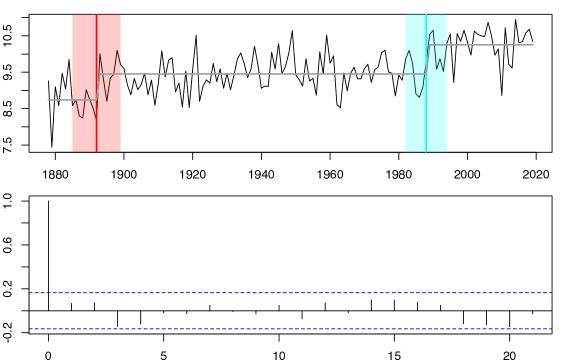
Figure 5: Top: Yearly average temperatures between 1878 and 2019 plotted together with the change points estimated by MoLP (vertical lines), shaded areas representing the $90\%$ uniform confidence intervals around the change points and piecewise constant mean (bold lines) Bottom: Autocorrelations of the data after the two mean shifts are removed.

The Hadley Centre central England temperature (HadCET) dataset (Parker et al.,, 1992) contains the mean daily and monthly temperatures representative of a roughly triangular area enclosed by Lancashire, London and Bristol, UK. We analyse the yearly average of the monthly mean temperatures of the period of 1878–2019 ($n=142$) for change points using MoLP (applied with the significance level $0.2$ and other tuning parameters set at their default values) and derive their 90% CIs, see Table 3 and also the top panel of Figure 5 for the visualisation of the uniform CIs. The bottom panel of Figure 5 shows that after the mean shifts are accounted for, the series exhibits little autocorrelations and thus justifies the use of the proposed bootstrap methodology. The second change point detected at 1987/88 coincides with the global regime shift in Earth’s biophysical systems identified around 1987 (Reid et al.,, 2016), which is attributed to anthropogenic warming and a volcanic eruption.

Table 3: Pointwise and uniform $90\%$ CIs obtained with $\widehat{\theta}_{1}=1892$ and $\widehat{\theta}_{2}=1988$.

	pointwise	uniform
$\theta_{1}$	$[1887,1897]$	$[1885,1899]$
$\theta_{2}$	$[1984,1992]$	$[1983,1993]$

6 Conclusions

In this paper we rigorously analyse a bootstrap method for the construction of CIs for the location of change points obtained from MOSUM-based procedures, both theoretically and in simulation studies. We show that for local changes (i.e. $d_{j}=d_{j,n}\to 0$), the limit distributions of change point estimators are continuous as a functional of a Wiener process with drift, while those for the fixed changes remain discrete. Such results hold under mild assumptions made in (2) that permit non-Gaussianity and heavy-tails, and could even be extended to serially correlated errors as discussed in Section 4.2. Both our theoretical investigation into the asymptotic distribution of the change point estimators and bootstrap CI construction, are based on the oracle estimators in (4) and (6), with the former tied to MOSUM-based change point estimators as noted in Assumption 2.1. To the best of our knowledge, in the fixed change case, there was no proof of the validity of the bootstrap procedure in the literature even for the AMOC setting with CUSUM-based estimators. The proof requires non-standard steps due to the non-Gaussianity of the limit distribution of the change point estimators. Despite the distinct behaviour of the limit distributions for fixed and local changes, the proposed bootstrap procedure adapts to the magnitude of the change without knowing the regime it belongs to.

Numerical studies show that the bootstrap works well with the oracle estimators, and only slightly more conservative when constructed with the estimators which are obtained with an additional model selection step (and thus accessible in practice). The results suggest that the bootstrap CIs behave well in the presence of heavy-tailed errors, and also in comparison with competing methodologies. Both the implementation of the proposed bootstrap methodology as well as the multiple change point detection procedure adopted for simulation studies (MoLP) are available in the R package mosum (Meier et al., 2021a, ).

Appendix A Proofs

A.1 Proof of Theorem 3.1

Assumptions A.1 b) and c) of Eichinger and Kirch, (2018) are fulfilled in the situation considered here; see Komlós et al., (1975, 1976) and Major, (1976) for the invariance principle (although for the proof of this theorem, the functional central limit theorem is sufficient), and Theorem 3.7.8 of Stout and Stout, (1974), for the moment assumption on the sums of the errors. First, note that

$$\widetilde{\theta}_{j}=\arg\max_{k:\,|k-\theta_{j}|\leq G_{j}}V_{k,n}(G_{j}),\quad\text{where}\quad V_{k,n}(G_{j})=(T_{k,n}(G_{j}))^{2}-(T_{\theta_{j},n}(G_{j}))^{2}.$$

The proof of Theorem 3.2 in Eichinger and Kirch, (2018) shows that for any $c>1$

$$\mathsf{P}\left(|\widetilde{\theta}_{j}-\theta_{j}|>c\sigma^{2}d_{j}^{-2}\right)\leq\mathsf{P}\left(\max_{|k-\theta_{j}|>c\sigma^{2}d_{j}^{-2}}V_{k,n}(G_{j})\geq\max_{|k-\theta_{j}|\leq c\sigma^{2}d_{j}^{-2}}V_{k,n}(G_{j})\right)$$

$$\leq O(c^{-1})+o(1).$$ (12)

Therefore,

$$\mathsf{P}\left(\frac{d_{j}^{2}(\widetilde{\theta}_{j}-\theta_{j})}{\sigma^{2}}\leq x\right)=\mathsf{P}\left(-c\leq\frac{d_{j}^{2}(\widetilde{\theta}_{j}-\theta_{j})}{\sigma^{2}}\leq x\right)+O(c^{-1})+o(1).$$

Furthermore by Lemma 5.2 in Eichinger and Kirch, (2018) and the decomposition of $V_{k,n}(G_{j})$ as given in their (5.8), it holds for any $k$ satisfying $-c\leq\sigma^{-2}d_{j}^{2}(k-\theta_{j})<0$,

$$V_{k,n}(G_{j}) =-d_{j}^{2}|\theta_{j}-k|-d_{j}\left(\sum_{t=k-G_{j}+1}^{\theta_{j}-G_{j}}\varepsilon_{t}-2\sum_{t=k+1}^{\theta_{j}}\varepsilon_{t}+\sum_{t=k+G_{j}+1}^{\theta_{j}+G_{j}}\varepsilon_{t}\right)+o_{P}(1)$$ (13)

$$=:\widetilde{V}_{k,n}(G_{j})+o_{P}(1),$$

where the $o_{P}(1)$ term is uniform over $\theta_{j}-G_{j}\leq k<\theta_{j}$, and

$$\left\{d_{j}\left(\sum_{t=k-G_{j}+1}^{\theta_{j}-G_{j}}\varepsilon_{t}-2\sum_{t=k+1}^{\theta_{j}}\varepsilon_{t}+\sum_{t=k+G_{j}+1}^{\theta_{j}+G_{j}}\varepsilon_{t}\right):\,k=\theta_{j}-1,\ldots,\theta_{j}-c\sigma^{2}d_{j}^{-2}\right\}$$ (14)

$$\overset{\mathcal{D}}{=}\left\{U_{n}(\ell)=d_{j}\left(\sum_{t=\ell}^{-1}\varepsilon_{t}^{(1)}-2\sum_{t=\ell}^{-1}\varepsilon_{t}^{(2)}+\sum_{t=\ell}^{-1}\varepsilon_{t}^{(3)}\right):\,\ell=-1,\ldots,-c\sigma^{2}d_{j}^{-2}\right\}.$$

Analogous assertions hold for $\theta_{j}<k\leq\theta_{j}+G_{j}$.

So far, the preceding arguments hold for both the local and the fixed change cases. Now, the proof for the local change ($d_{j}=d_{j,n}\to 0$) in (a) is concluded as in the proof of Theorem 3.3 in Eichinger and Kirch, (2018) by making use of the following functional central limit theorem

$$\left\{\frac{U_{n}(\lfloor s\sigma^{2}d_{j}^{-2}\rfloor)}{\sigma^{2}}:\,-c\leq s\leq c\right\}\overset{D[-c,c]}{\longrightarrow}\{\sqrt{6}\,W(s),\,-c\leq s\leq c\}.$$

We elaborate on the proof here in order to highlight the difference between the local and the fixed change cases. Note that

$$\mathsf{P}\left(-c\leq\frac{d_{j}^{2}(\widetilde{\theta}_{j}-\theta_{j})}{\sigma^{2}}\leq x\right)$$

$$=\mathsf{P}\left(\max_{-c\leq d_{j}^{2}(k-\theta_{j})/\sigma^{2}\leq x}\widetilde{V}_{k,n}(G_{j})\geq\max_{x<d_{j}^{2}(k-\theta_{j})/\sigma^{2}\leq c}\widetilde{V}_{k,n}(G_{j})+o_{P}(1)\right).$$

Thus, for any $\eta>0$, we obtain

$$\mathsf{P}\left(-c\leq\frac{d_{j}^{2}(\widetilde{\theta}_{j}-\theta_{j})}{\sigma^{2}}\leq x\right)$$

$$\leq\mathsf{P}\left(\max_{-c\leq d_{j}^{2}(k-\theta_{j})/\sigma^{2}\leq x}\widetilde{V}_{k,n}(G_{j})\geq\max_{x<d_{j}^{2}(k-\theta_{j})/\sigma^{2}\leq c}\widetilde{V}_{k,n}(G_{j})-\eta\right)+o(1)$$ (15)

$$\to\mathsf{P}\left(\max_{-c\leq s\leq x}\left(-|s|-\sqrt{6}W(s)\right)\geq\max_{x<s\leq c}\left(-|s|-\sqrt{6}W(s)\right)-\eta\right)$$

as well as

$$\mathsf{P}\left(-c\leq d_{j}^{2}\frac{\widetilde{\theta}_{j}-\theta_{j}}{\sigma^{2}}\leq x\right)$$

$$\geq\mathsf{P}\left(\max_{-c\leq d_{j}^{2}(k-\theta_{j})/\sigma^{2}\leq x}\widetilde{V}_{k,n}(G_{j})\geq\max_{x<d_{j}^{2}(k-\theta_{j})/\sigma^{2}\leq c}\widetilde{V}_{k,n}(G_{j})+\eta\right)+o(1)$$ (16)

$$\to\mathsf{P}\left(\max_{-c\leq s\leq x}\left(-|s|-\sqrt{6}W(s)\right)\geq\max_{x<s\leq c}\left(-|s|-\sqrt{6}W(s)\right)+\eta\right).$$

Since the maximum of a Wiener process with drift has a continuous distribution, the limits of both the upper and lower bounds on (15)–(16) coincide on letting $\eta\to 0$ with

$$\mathsf{P}\left(-c\leq{\arg\max}_{-c\leq s\leq c}\left(W(s)-|s|/\sqrt{6}\right)\leq x\right),$$

such that the results follows by letting $c\to\infty$.

The proof of the fixed change case proceeds similarly, apart from that $U_{n}(\ell)$ already coincides with the limit distribution such that no additional functional central limit theorem is necessary. Hence, the upper and lower bounds in (15)–(16) coincide as $\eta\to 0$ as long as the maximum over $U_{n}(\ell)$ (plus drift) has a continuous distribution, which in turn holds provided that $\{\varepsilon_{t}\}$ have a continuous distribution. On the other hand, for discrete distributions where ties in the maximum can occur with positive probability, the two bounds are not guaranteed to converge. In fact, when ties in the maximum exist, the $\arg\max$ over the corresponding functional of $\{\widetilde{V}_{k,n}(G_{j})\}$ (always picking the first of the two maximisers) can differ from the $\arg\max$ over the functional of $\{V_{k,n}(G_{j})\}$, since the $o_{P}(1)$ term can make the second maximum strictly larger than the first for all $n$ (with the two coinciding in the limit).

The assertion for (c) follows immediately from (a) and (b) by noting that the maximisers involve different errors provided that $4G_{j}<\delta_{j}$ for all $j=1,\ldots,q$, and thus are independent.

A.2 Proof of Theorem 3.2

In this section, the notations $o_{P}$ and $O_{P}$ are reserved for the functionals of the original observations $X_{1},\ldots,X_{n}$, which are deterministic given those observations. Also, in order to facilitate the proofs below, we always condition on the following set

$$\mathcal{M}_{j}=\mathcal{M}_{j,n}= \left\{\widehat{\theta}_{j-1}>\theta_{j-2},\quad\widehat{\theta}_{j+1}<\theta_{j+2},\quad|\widehat{\theta}_{j}-\theta_{j}|<\frac{1}{3}\delta_{j}\right.$$

$$\left.\quad\text{and}\quad|\widehat{\theta}_{i}-\theta_{i}|<\frac{1}{3}|\theta_{j}-\theta_{i}|\text{ for }i=j-1,j+1,\right\}.$$ (17)

Under Assumption 3.1, it holds that $\mathsf{P}(\mathcal{M}_{j,n})\to 1$ for each $j$. In addition, we use the notations $\mathsf{E}^{*}(\cdot)=\mathsf{E}(\cdot|X_{1},\ldots,X_{n})$ and $\mathsf{var}^{*}(\cdot)=\mathsf{var}(\cdot|X_{1},\ldots,X_{n})$.

A.2.1 Auxiliary lemmas

In what follows, we denote for $\widehat{\theta}_{j-1}<t\leq\widehat{\theta}_{j}$,

$$\varepsilon_{t}^{*}=X_{t}^{*}-\mathsf{E}^{*}(X_{t}^{*}).$$ (18)

Lemma A.1.

Let (1)–(2) and Assumption 3.1 hold for a given $j$.

1. It holds

   $$\mathsf{E}^{*}(X^{*}_{t})=\begin{cases}\bar{X}_{\widehat{\theta}_{j-1},\widehat{\theta}_{j}}=\mathsf{E}(X_{\theta_{j}})+o_{P}(|d_{j}|)&\text{for }\widehat{\theta}_{j-1}<t\leq\widehat{\theta}_{j},\\ \bar{X}_{\widehat{\theta}_{j},\widehat{\theta}_{j+1}}=\mathsf{E}(X_{\theta_{j+1}})+o_{P}(|d_{j}|)&\text{for }\widehat{\theta}_{j}<t\leq\widehat{\theta}_{j+1}.\end{cases}$$

   In particular, $d_{j}^{*}=\widehat{d}_{j}=\bar{X}_{\widehat{\theta}_{j},\widehat{\theta}_{j+1}}-\bar{X}_{\widehat{\theta}_{j-1},\widehat{\theta}_{j}}=d_{j}+o_{P}(|d_{j}|)$.

2. It holds that $(\sigma^{*}_{t})^{2}=\mathsf{var}^{*}(X^{*}_{t})=\mathsf{var}^{*}(\varepsilon^{*}_{t})=\sigma^{2}+o_{P}(1)$ with $(\sigma^{*}_{t})^{2}$ being constant over each segment $\widehat{\theta}_{j-1}<t\leq\widehat{\theta}_{j}$. Then, the $o_{P}(1)$ term is uniform as long as only finitely many segments are involved.

Proof.

For the proof of (a), note that from the Hájek-Rényi inequality for i.i.d. random variables, it holds

$$\max_{1\leq k\leq\frac{4}{3}(\theta_{j}-\theta_{j-1})}\left|\sum_{t=\theta_{j}-k}^{\theta_{j}}\varepsilon_{t}\right|=O_{P}(\sqrt{\theta_{j}-\theta_{j-1}}),\quad\max_{1\leq k<\frac{1}{3}(\theta_{j}-\theta_{j-1})}\left|\sum_{t=\theta_{j}+1}^{\theta_{j}+k}\varepsilon_{t}\right|=O_{P}(\sqrt{\theta_{j}-\theta_{j-1}}).$$ (19)

Then on $\mathcal{M}_{j}$ defined in (17), the following decomposition holds

$$\mathsf{E}^{*}(X_{t}^{*})=\bar{X}_{\widehat{\theta}_{j-1},\widehat{\theta}_{j}} =\mathsf{E}(X_{\theta_{j}})+\frac{1}{\widehat{\theta}_{j}-\widehat{\theta}_{j-1}}\sum_{\widehat{\theta}_{j-1}+1}^{\widehat{\theta}_{j}}\varepsilon_{t}$$

$$\qquad-\frac{d_{j-1}(\theta_{j-1}-\widehat{\theta}_{j-1})\mathbb{I}_{\{\theta_{j-1}>\widehat{\theta}_{j-1}\}}}{\widehat{\theta}_{j}-\widehat{\theta}_{j-1}}+\frac{d_{j}(\widehat{\theta}_{j}-\theta_{j})\mathbb{I}_{\{\widehat{\theta}_{j}>\theta_{j}\}}}{\widehat{\theta}_{j}-\widehat{\theta}_{j-1}}$$

$$=\mu_{j}+O_{P}((\theta_{j}-\theta_{j-1})^{-1/2})+o_{P}(|d_{j}|)=\mu_{j}+o_{P}(|d_{j}|),$$ (20)

from the bounds in (19), Assumption 3.1 and that $d_{j}^{2}(\theta_{j}-\theta_{j-1})\to\infty$. Analogous assertions hold when $t>\widehat{\theta}_{j}$, completing the proof of (a). Consequently, with $o_{P}(1)$ uniformly in $\widehat{\theta}_{j-1}<t\leq\widehat{\theta}_{j}$

$$\widehat{\varepsilon}_{t}=X_{t}-\bar{X}_{\widehat{\theta}_{j-1},\widehat{\theta}_{j}}=\varepsilon_{t}+o_{P}(1)-d_{j-1}\mathbb{I}_{\{\widehat{\theta}_{j-1}<t\leq\theta_{j-1}\}}+d_{j}\mathbb{I}_{\{\theta_{j}<t\leq\widehat{\theta}_{j}\}}.$$ (21)

For the proof of (b), note that for $\widehat{\theta}_{j-1}<t\leq\widehat{\theta}_{j}$,

$$\mathsf{var}^{*}(\varepsilon^{*}_{t}) =\frac{1}{\widehat{\theta}_{j}-\widehat{\theta}_{j-1}}\sum_{t=\widehat{\theta}_{j-1}+1}^{\widehat{\theta}_{j}}\left(X_{t}-\bar{X}_{\widehat{\theta}_{j-1},\widehat{\theta}_{j}}\right)^{2}=\frac{1}{\widehat{\theta}_{j}-\widehat{\theta}_{j-1}}\sum_{t=\widehat{\theta}_{j-1}+1}^{\widehat{\theta}_{j}}\varepsilon_{t}^{2}+o_{P}(1)=\sigma^{2}+o_{P}(1),$$

by Assumption 3.1 and the law of large numbers, where similar arguments as those adopted in (20) have been used for the terms including the indicators. ∎

The following lemma is the bootstrap analogue to Lemma 5.2 of Eichinger and Kirch, (2018).

Lemma A.2.

Let the assumptions in Theorem 3.2 hold for a given $j$. Then for any sequences $\beta_{n}>0$ and $\xi_{n}\geq 1$, it holds:

1. $\displaystyle\mathsf{P}^{*}\left(\max_{\widehat{\theta}_{j}-G_{j}\leq k\leq\widehat{\theta}_{j}-\xi_{n}}\frac{\left|T_{\widehat{\theta}_{j},n}(G_{j};\varepsilon^{*})-T_{k,n}(G_{j};\varepsilon^{*})\right|}{\widehat{\theta}_{j}-k}>\beta_{n}(1+o_{P}(1))\right)=O_{P}\left(\left(\beta_{n}^{2}G_{j}\xi_{n}\right)^{-1}\right)$.

2. $\displaystyle\mathsf{P}^{*}\left(\max_{\widehat{\theta}_{j}-\xi_{n}\leq k\leq\widehat{\theta}_{j}}\left|T_{\widehat{\theta}_{j},n}(G_{j};\varepsilon^{*})-T_{k,n}(G_{j};\varepsilon^{*})\right|>\beta_{n}(1+o_{P}(1))\right)=O_{P}\left(\beta_{n}^{-2}\,\frac{\xi_{n}}{G_{j}}\right)$.

3. $\displaystyle\mathsf{P}^{*}\left(\max_{\widehat{\theta}_{j}-G_{j}\leq k\leq\widehat{\theta}_{j}-\xi_{n}}\left|T_{\widehat{\theta}_{j},n}(G_{j};\varepsilon^{*})+T_{k,n}(G_{j};\varepsilon^{*})\right|>\beta_{n}(1+o_{P}(1))\right)=O_{P}\left(\beta_{n}^{-2}\right)$.

Proof.

Some straightforward calculations show that for $k\leq\widehat{\theta}_{j}$, we have

$$T_{\widehat{\theta}_{j},n}(G_{j};\varepsilon^{*})-T_{k,n}(G_{j};\varepsilon^{*})=\frac{1}{\sqrt{2G_{j}}}\left(\sum_{t=k+G_{j}+1}^{\widehat{\theta}_{j}+G_{j}}\varepsilon^{*}_{t}+\sum_{t=k-G_{j}+1}^{\widehat{\theta}_{j}-G_{j}}\varepsilon^{*}_{t}-2\sum_{t=k+1}^{\widehat{\theta}_{j}}\varepsilon^{*}_{t}\right).$$ (22)

By the Hájek-Rényi inequality for i.i.d. random variables and Lemmas A.1 (b), the first summand in the RHS of (22) satisfies

$$\mathsf{P}^{*}\left(\max_{\widehat{\theta}_{j}-G_{j}\leq k\leq\widehat{\theta}_{j}-\xi_{n}}\left|\frac{\sum_{t=k+G_{j}+1}^{\widehat{\theta}_{j}+G_{j}}\varepsilon^{*}_{t}}{\widehat{\theta}_{j}-k}\right|>\beta_{n}(1+o_{P}(1))\sqrt{G_{j}}\right)=O_{P}(1)\frac{1}{\beta_{n}^{2}G_{j}\xi_{n}}\mathsf{var}^{*}(\varepsilon^{*}_{\widehat{\theta}_{j}+1})$$

$$=O_{P}\left((\beta_{n}^{2}G_{j}\xi_{n})^{-1}\right),$$

as well as

$$\mathsf{P}^{*}\left(\max_{\widehat{\theta}_{j}-\xi_{n}\leq k\leq\widehat{\theta}_{j}}\left|\sum_{t=k+G_{j}+1}^{\widehat{\theta}_{j}+G_{j}}\varepsilon^{*}_{t}\right|>\beta_{n}(1+o_{P}(1))\sqrt{G_{j}}\right)=O_{P}(1)\frac{\xi_{n}}{\beta_{n}^{2}G_{j}}\mathsf{var}^{*}(\varepsilon^{*}_{\widehat{\theta}_{j}+1})=O_{P}\left(\beta_{n}^{-2}\,\frac{\xi_{n}}{G_{j}}\right).$$

Analogous assertions hold for the other two summands in (22), which lead to (a) and (b). As for (c), noting that $T_{\widehat{\theta}_{j},n}(G_{j};\varepsilon^{*})+T_{k,n}(G_{j};\varepsilon^{*})=2T_{\widehat{\theta}_{j},n}(G_{j};\varepsilon^{*})+T_{k,n}(G_{j};\varepsilon^{*})-T_{\widehat{\theta}_{j},n}(G_{j};\varepsilon^{*})$, the arguments adopted in the proof of (b) and Chebyshev’s inequality lead to the conclusion. ∎

Lemma A.3.

Let (1)–(2) hold and suppose that the change point estimators satisfy Assumption 3.1 for a given $j$. Then, it holds for $\widehat{\theta}_{j-1}<t\leq\widehat{\theta}_{j+1}$,

$$\sup_{x\in\mathbb{R}}\left|\mathsf{P}^{*}(\varepsilon_{t}^{*}\leq x)-\mathsf{P}(\varepsilon_{1}\leq x)\right|\overset{\mathcal{P}}{\to}0.$$

Proof.

Denote $\widehat{F}_{a,b}(Z_{t};x)=(b-a)^{-1}\sum_{t=a+1}^{b}\mathbb{I}_{\{Z_{t}\leq x\}}$ and $F(x)=\mathsf{P}(\varepsilon_{1}\leq x)$. Then for $\widehat{\theta}_{j-1}<t\leq\widehat{\theta}_{j}$, the following decomposition holds on $\mathcal{M}_{j}$ defined in (17):

$$\left|\widehat{F}_{\widehat{\theta}_{j-1},\widehat{\theta}_{j}}\left(\varepsilon_{t}-d_{j-1}\mathbb{I}_{\{\widehat{\theta}_{j-1}<t\leq\theta_{j-1}\}}+d_{j}\mathbb{I}_{\{\theta_{j}<t\leq\widehat{\theta}_{j}\}};x\right)-F(x)\right|$$

$$\leq\left|\widehat{F}_{\widehat{\theta}_{j-1},\widehat{\theta}_{j}}\left(\varepsilon_{t}-d_{j-1}\mathbb{I}_{\{\widehat{\theta}_{j-1}<t\leq\theta_{j-1}\}}+d_{j}\mathbb{I}_{\{\theta_{j}<t\leq\widehat{\theta}_{j}\}};x\right)-\widehat{F}_{{\widehat{\theta}_{j-1},\widehat{\theta}_{j}}}(\varepsilon_{t};x)\right|$$

$$+\left|\widehat{F}_{{\widehat{\theta}_{j-1},\widehat{\theta}_{j}}}(\varepsilon_{t};x)-\widehat{F}_{{\theta_{j-1},\theta_{j}}}(\varepsilon_{t};x)\right|+\left|\widehat{F}_{{\theta_{j-1},\theta_{j}}}(\varepsilon_{t};x)-F(x)\right|=:D_{1}(x)+D_{2}(x)+o_{P}(1),$$

where the $o_{P}(1)$ holds uniformly in $x$ due to the Glivenko-Cantelli theorem. Furthermore,

$$\sup_{x}|D_{1}(x)|\leq\frac{1}{\widehat{\theta}_{j}-\widehat{\theta}_{j-1}}\left(|\widehat{\theta}_{j-1}-\theta_{j-1}|+|\widehat{\theta}_{j}-\theta_{j}|\right)=o_{P}(1)$$

by Assumption 3.1. Similarly, uniformly in $x$, we have

$$|D_{2}(x)|$$

$$\leq\left|\frac{1}{\theta_{j}-\theta_{j-1}}-\frac{1}{\widehat{\theta}_{j}-\widehat{\theta}_{j-1}}\right|\;\left|\sum_{t=\theta_{j-1}+1}^{\theta_{j}}\mathbb{I}_{\{\varepsilon_{t}\leq x\}}\right|+\frac{1}{\widehat{\theta}_{j}-\widehat{\theta}_{j-1}}\left|\sum_{t=\theta_{j-1}+1}^{\theta_{j}}\mathbb{I}_{\{\varepsilon_{t}\leq x\}}-\sum_{t=\widehat{\theta}_{j-1}+1}^{\widehat{\theta}_{j}}\mathbb{I}_{\{\varepsilon_{t}\leq x\}}\right|$$

$$\leq\frac{2}{\widehat{\theta}_{j}-\widehat{\theta}_{j-1}}\left(|\widehat{\theta}_{j-1}-\theta_{j-1}|+|\widehat{\theta}_{j}-\theta_{j}|\right)=o_{P}(1).$$

Analogous assertions hold for $t>\widehat{\theta}_{j}$ which concludes the proof. ∎

Proof of Theorem 3.2.

The proof proceeds analogously as the proof of Theorem 3.1, replacing the sample quantities therein with their bootstrap counterparts and Lemma 5.2 of Eichinger and Kirch, (2018) with Lemma A.2. Lemma A.1 (b) and Lemma 5.1 in Hušková and Kirch, (2008) replace the standard functional central limit theorem adopted in the proof of Theorem 3.1 (a) where $d_{j}=d_{j,n}\to 0$, while Lemma A.3 is required to deal with the fixed change situation.

To elaborate, consider $V_{k,n}^{*}(G_{j})=(T_{k,n}(G_{j};X^{*}))^{2}-(T_{\theta_{j},n}(G_{j};X^{*}))^{2}$. Then, standard arguments analogous to those adopted in the proof of Theorem 3.2 in Eichinger and Kirch, (2018) yield

$$\mathsf{P}^{*}\left(|\widetilde{\theta}_{j}^{*}-\widehat{\theta}_{j}|>c\sigma^{2}d_{j}^{-2}\right)\leq\mathsf{P}^{*}\left(\max_{|k-\widehat{\theta}_{j}|>c\sigma^{2}d_{j}^{-2}}V^{*}_{k,n}(G_{j})\geq\max_{|k-\widehat{\theta}_{j}|\leq c\sigma^{2}d_{j}^{-2}}V^{*}_{k,n}(G_{j})\right)$$

$$\leq O_{P}(c^{-1})+o_{P}(1).$$

This follows from Lemma A.2 where the additional $1+o_{P}(1)$ factor therein is needed to account for $\widehat{d}_{j}=d_{j}(1+o_{P}(1))$, which follows from Lemma A.1 (a). Additionally, for $-c\leq\sigma^{-2}d_{j}^{2}(k-\widehat{\theta}_{j})<0$,

$$V^{*}_{k,n}(G_{j}) =-d_{j}^{2}(1+o_{P}(1))|\widehat{\theta}_{j}-k|$$

$$\quad-d_{j}(1+o_{P}(1))\,\left(\sum_{t=k-G_{j}+1}^{\widehat{\theta}_{j}-G_{j}}\varepsilon^{*}_{t}-2\sum_{t=k+1}^{\widehat{\theta}_{j}}\varepsilon^{*}_{t}+\sum_{t=k+G_{j}+1}^{\widehat{\theta}_{j}+G_{j}}\varepsilon^{*}_{t}\right)+{R^{*(1)}_{n}}(k)$$

$$=-d_{j}^{2}|\widehat{\theta}_{j}-k|-d_{j}\,\left(\sum_{t=k-G_{j}+1}^{\widehat{\theta}_{j}-G_{j}}\varepsilon^{*}_{t}-2\sum_{t=k+1}^{\widehat{\theta}_{j}}\varepsilon^{*}_{t}+\sum_{t=k+G_{j}+1}^{\widehat{\theta}_{j}+G_{j}}\varepsilon^{*}_{t}\right)+{R^{*(1)}_{n}}(k)+{R^{*(2)}_{n}}(k)$$

$$=:\widetilde{V}_{k,n}^{*}(G_{j})+R_{n}^{*}(k).$$

It holds by arguments analogous to those in the proof of Theorem 3.1 (which make use of the decomposition in Equation (5.8) of Eichinger and Kirch, (2018)) for ${R^{*(1)}_{n}}(k)$, and from the (conditional) stochastic boundedness of $U_{n}^{*}(\ell)$ defined below for ${R^{*(2)}_{n}}(k)$, that for any $\tau>0$,

$$\mathsf{P}^{*}\left(\sup_{k:\,|k-\widehat{\theta}_{j}|\leq c\sigma^{2}d_{j}^{-2}}|R_{n}^{*}(k)|\geq\tau\right)=o_{P}(1).$$

On $\mathcal{M}_{j}$ and for $n$ large enough such that $c\sigma^{2}d_{j}^{-2}<G_{j}$, we have

$$\left\{d_{j}\left(\sum_{t=k-G_{j}+1}^{\widehat{\theta}_{j}-G_{j}}\varepsilon^{*}_{t}-2\sum_{t=k+1}^{\widehat{\theta}_{j}}\varepsilon^{*}_{t}+\sum_{t=k+G_{j}+1}^{\widehat{\theta}_{j}+G_{j}}\varepsilon^{*}_{t}\right):k=\widehat{\theta}_{j}-1,\ldots,\widehat{\theta}_{j}-c\sigma^{2}d_{j}^{-2}\,\Big{|}\,X_{1},\ldots,X_{n}\right\}$$

$$\overset{\mathcal{D}}{=}\left\{U_{n}^{*}(\ell)=d_{j}\left(\sum_{t=\ell}^{-1}(\varepsilon^{*}_{t})^{(1)}-2\sum_{t=\ell}^{-1}(\varepsilon_{t}^{*})^{(2)}+\sum_{t=\ell}^{-1}(\varepsilon_{t}^{*})^{(3)}\right):\ell=-1,\ldots,-c\sigma^{2}d_{j}^{-2}\,\Big{|}\,X_{1},\ldots,X_{n}\right\},$$

where $\{(\varepsilon^{*}_{t})^{(3)}\}$ are distributed according to $\{\varepsilon^{*}_{t},\,\widehat{\theta}_{j}<t\leq\widehat{\theta}_{j+1}\}$ and independent of $\{(\varepsilon^{*}_{t})^{(i)}\}$, $i=1,2$, which in turn are independent copies of $\{\varepsilon^{*}_{t},\,\widehat{\theta}_{j-1}<t\leq\widehat{\theta}_{j}\}$. Similar assertions hold for $k$ satisfying $0\leq\sigma^{-2}d_{j}^{2}(k-\widehat{\theta}_{j})\leq c$: Here, $\{(\varepsilon^{*}_{t})^{(1)}\}$ are distributed according to $\{\varepsilon^{*}_{t},\,\widehat{\theta}_{j-1}<t\leq\widehat{\theta}_{j}\}$ and independent of $\{(\varepsilon^{*}_{t})^{(i)}\}$, $i=2,3$, which are independent copies of $\{\varepsilon^{*}_{t},\,\widehat{\theta}_{j}<t\leq\widehat{\theta}_{j+1}\}$, and all of $\{(\varepsilon^{*}_{t})^{(i)},\,t=1,\ldots,c\sigma^{2}d_{j}^{-2},\,i=1,2,3\}$, are independent of $\{(\varepsilon^{*}_{t})^{(i)},\,t=-1,\ldots,-c\sigma^{2}d_{j}^{-2},\,i=1,2,3\}$.

Arguments so far hold in the local and the fixed change cases. Now, in the case of the local change ($d_{j}=d_{j,n}\to 0$) as in (a) the proof is concluded as in the proof of Theorem 3.1 (a) by replacing the functional central limit theorem there with a version suitable for the triangular arrays present in the bootstrap distribution as given in Lemma 5.1 of Hušková and Kirch, (2008), where the assumptions therein are fulfilled due to Lemma A.1 (b). Hence for any $x$, it holds

$$\mathsf{P}^{*}\left(\frac{d_{j}^{2}(\widetilde{\theta}^{*}_{j}-\widehat{\theta}_{j})}{\sigma^{2}}\leq x\right)\overset{\mathcal{P}}{\to}\mathsf{P}\left(\arg\max_{s\in\mathbb{R}}\left\{W_{s}-|s|/\sqrt{6}\right\}\leq x\right).$$

For the fixed change case, unlike in the proof of Theorem 3.1 where the distribution in the limit is the same as that of $U_{n}(\ell)$ such that no additional limit theorem is required, here we do need that $U_{n}^{*}(\ell)$ converges to $U_{n}(\ell)$ in an appropriate sense. Due to the cutting technique employed in this proof, the required convergence follows from Lemma A.3 as below: First, by Lemma A.3 in combination with (conditional) independence under the bootstrap distribution and Lemma A.1, it holds with $L=c\sigma^{2}d_{j}^{-2}$ (which is constant for fixed $d_{j}$) for any $x_{t}^{(i)}$:

$$\mathsf{P}^{*}\left((\varepsilon_{t}^{*})^{(i)}\leq x_{t}^{(i)},\,|t|=1,\ldots,L,\,i=1,2,3\right)\overset{\mathcal{P}}{\to}\mathsf{P}\left(\varepsilon_{t}^{(i)}\leq x_{t}^{(i)},\,|t|=1,\ldots,L,\,i=1,2,3\right)$$ (23)

with $\varepsilon_{t}^{(i)}$ as in Theorem 3.1 (b), such that for any $x_{\ell}$,

$$\mathsf{P}^{*}\left(U_{n}^{*}(\ell)\leq x_{\ell}:\,\ell=-1,\ldots,-L\right)\overset{\mathcal{P}}{\to}\mathsf{P}\left(U_{n}(\ell)\leq x_{\ell}:\,\ell=-1,\ldots,-L\right).$$

The proof can then be concluded as in the proof of Theorem 3.1 on noting that the errors in the limit distribution have a continuous distribution. ∎

Appendix B MOSUM-based procedures for multiple change point estimation

In Eichinger and Kirch, (2018), simultaneous estimation of multiple change points via a single-scale MOSUM procedure has been considered which, for a bandwidth $G=G_{n}$, estimates the locations of the change points as where significant local maxima of the MOSUM statistics in (3) are attained. For the identification of these significant local maxima, different criteria have been considered. One such a criterion regards $\widehat{\theta}$ as a change point estimator when it is the local maximiser of the MOSUM statistic within its $\lfloor\eta G\rfloor$-radius for some $\eta\in(0,1)$, and $|T_{\widehat{\theta},n}(G;X)|>\widehat{\sigma}_{n}\;D_{n}(G;\alpha)$. Here, $D_{n}(G;\alpha)$ is a threshold that controls asymptotically the family-wise error rate (of $\sigma^{-1}|T_{k,n}(G;\varepsilon)|$ exceeding $D_{n}(G;\alpha)$ over $G\leq k\leq n-G$) at the significance level $\alpha\in(0,1)$, and $\widehat{\sigma}_{n}^{2}$ a suitable estimator of $\sigma^{2}$. In the context of testing for a single change point, permutation methods have been proposed as an alternative to the asymptotic threshold (Antoch and Hušková,, 2001; Hušková,, 2004). Such an approach has also been suggested by Arias-Castro et al., (2018) when adopting scan statistics for anomaly detection.

Let the set of estimators obtained as described above be denoted by $\widehat{\Theta}(G)=\{\widehat{\theta}_{j}(G),\,1\leq j\leq\widehat{q}_{n}(G)\}$. Corollary D.2 of Cho and Kirch, 2021b , improving upon Theorem 3.2 of Eichinger and Kirch, (2018), shows that $\widehat{\Theta}(G)$ satisfies:

$$\mathsf{P}\left(\widehat{q}_{n}(G)=q_{n},\,\widehat{\theta}_{j}(G)=\widetilde{\theta}_{j},\,j=1,\ldots,q_{n},\text{ and }\max_{1\leq j\leq q_{n}}d_{j}^{2}|\widehat{\theta}_{j}(G)-\theta_{j}|\leq\rho_{n}\right)\to 1$$ (24)

under mild assumptions on $\{\varepsilon_{t}\}$ permitting heavy-tails and serial dependence, for a suitable bandwidth $G$. The conditions on $G$ depend on the moments of the error sequence on the one hand (such that $G$ can be smaller as $\nu$ in (2) increases) as well as on the distance between neighbouring change points (i.e. $2G<\min_{1\leq j\leq q_{n}}\delta_{j}$) on the other hand. We require the size of the changes to be sufficiently large such that $\min_{1\leq j\leq q_{n}}d_{j}^{2}G\geq D_{n}$ with $D_{n}\to\infty$ at an appropriate rate in relation to the behaviour of $\{\varepsilon_{t}\}$ and, the resulting localisation rate satisfies $D_{n}^{-1}\rho_{n}\to 0$. This, together with the condition on the size of the changes and (24), shows that Assumptions 2.1 and 3.1 are fulfilled by $\widehat{\Theta}(G)$ with an appropriately chosen $G$.

In the important special case where $q_{n}=q$ is finite (as in Theorems 3.1 (c) and 3.2 (c)), the consistency result in (24) holds for $\rho_{n}$ that diverges at an arbitrarily slow rate, i.e. $\max_{1\leq j\leq q}d_{j}^{2}|\widehat{\theta}_{j}(G)-\theta_{j}|=O_{P}(1)$. Theorem 3.1 is closely related to the later result, not only showing that this rate is exact but also deriving the corresponding (non-degenerate) limit distribution. In fact, this localisation rate is minimax optimal in the multiple change point detection problem in (1) (see Verzelen et al., (2020)).

Generally speaking, this single-scale MOSUM procedure performs best with the bandwidth chosen as large as possible while avoiding to have more than one change point within the moving window at any time. Therefore, it lacks adaptivity when the change points are heterogeneous, i.e. when the data sequence contains both large changes over short intervals and small changes over long intervals of stationarity. In such a situation, applying the MOSUM procedure with a range of bandwidths, and then combining information across the multiple bandwidths, is one way of addressing this lack of adaptivity of the single-scale MOSUM procedure, at the cost of requiring a more complicated model selection procedure. The results in this paper take into account the possibility of using different bandwidths $G_{j}$ for the detection of individual $\theta_{j},\,j=1,\ldots,q_{n}$, see (4).

One such model selection procedure is the localised pruning proposed by Cho and Kirch, 2021b . When applied to the set of candidate change point estimators generated by the multiscale MOSUM procedure, it returns $\widehat{\Theta}=\{\widehat{\theta}_{j},\,1\leq j\leq\widehat{q}_{n}\}$ that achieves consistency by correctly estimating the number of change points $q_{n}$ as well as ‘almost’ inheriting the localisation property of $\widetilde{\theta}_{j}$, in the sense that $\max_{1\leq j\leq q_{n}}d_{j}^{2}|\widehat{\theta}_{j}-\theta_{j}|=O_{P}(\nu_{n}\rho_{n})$ with $\rho_{n}$ as in (24) for $\nu_{n}\to\infty$ at an arbitrary rate (see Corollary 4.2 in Cho and Kirch, 2021b ), when the set of bandwidths is suitably chosen. Furthermore, Cho and Kirch, 2021b formulate a rigorous framework permitting the aforementioned heterogeneity in change points and show that, under such a general setting, the multiscale MOSUM procedure combined with the localised pruning (termed MoLP in Section 5.2.2) is (almost) minimax optimal in terms of both separation (related to correctly estimating the number of change points) and localisation rates when $\{\varepsilon_{t}\}$ are i.i.d. sub-Gaussian or when $q_{n}$ is finite.

For algorithmic descriptions of the above procedures and further information about the R package mosum implementing them, see Meier et al., 2021b .

Appendix C Additional simulation results

In this section, we provide additional simulation results obtained with $\{\varepsilon_{t}\}$ following Gaussian distributions (Appendix C) as in Section 5, and $t_{5}$ distributions (Appendix C.2) for the five test signals, see Figure 6 for illustration. We keep the signal-to-noise ratio constant across the two scenarios. When generating bootstrap CIs with the additional model selection step using MoLP procedure, we apply a slightly larger penalty of $\log^{1.1}(n)$ when the errors are generated from $t_{5}$ distributions, in place of $\log^{1.01}(n)$ recommended by default and adopted for the Gaussian errors, for the localised pruning procedure of Cho and Kirch, 2021b ; all other tuning parameters are set identically.

As noted in Section 5, the bootstrap CIs constructed with the oracle estimators $\widetilde{\theta}_{j}$ closely attain the desired confidence level while those constructed with the estimators obtained from the additional model selection step tend to be more conservative, and we observe little difference in their behaviour whether $\{\varepsilon_{t}\}$ follow Gaussian distributions or $t_{5}$ distributions.

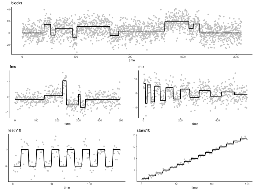
Figure 6: Realisations from the blocks, fms, mix, teeth10 and stairs10 test signals from Fryzlewicz, (2014) with Gaussian errors.

C.1 Gaussian errors

C.1.1 Bootstrap CIs constructed with the oracle estimators in (4)

Figure 7: blocks with $\vartheta=1$.

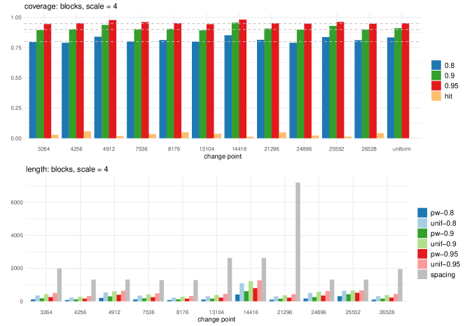
Figure 8: blocks with $\vartheta=4$.

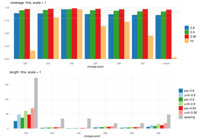
Figure 9: Bootstrap CIs constructed with the oracle estimators in (4): fms with $\vartheta=1$.

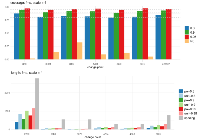
Figure 10: Bootstrap CIs constructed with the oracle estimators in (4): fms with $\vartheta=4$.

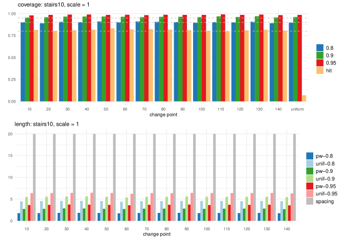
Figure 11: Bootstrap CIs constructed with the oracle estimators in (4): stairs10 with $\vartheta=1$.

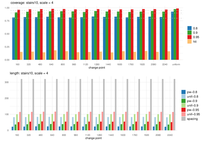
Figure 12: Bootstrap CIs constructed with the oracle estimators in (4): stairs10 with $\vartheta=4$.

C.1.2 Bootstrap CIs constructed with model selection

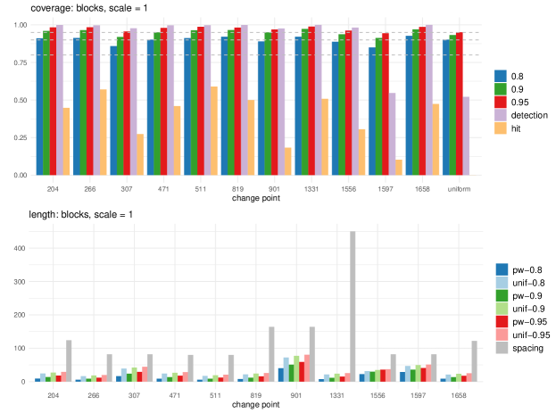
Figure 13: Bootstrap CIs constructed with model selection: blocks with $\vartheta=1$.

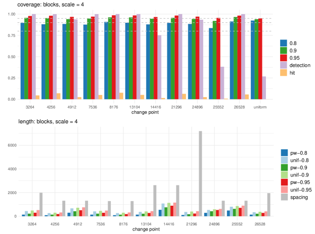
Figure 14: Bootstrap CIs constructed with model selection: blocks with $\vartheta=4$.

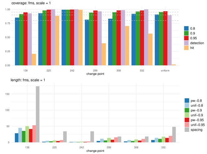
Figure 15: Bootstrap CIs constructed with model selection: fms with $\vartheta=1$.

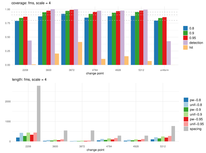
Figure 16: Bootstrap CIs constructed with model selection: fms with $\vartheta=4$.

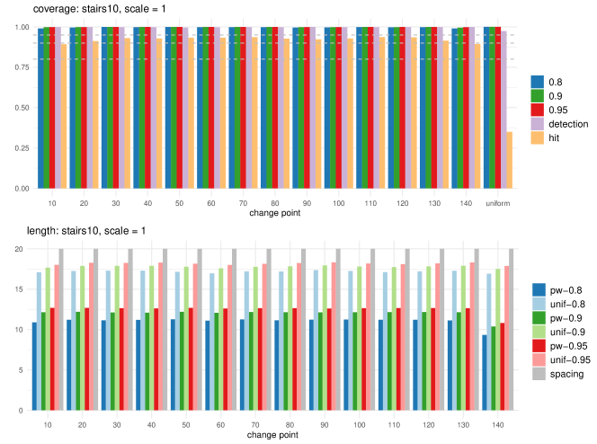
Figure 17: Bootstrap CIs constructed with model selection: stairs10 with $\vartheta=1$.

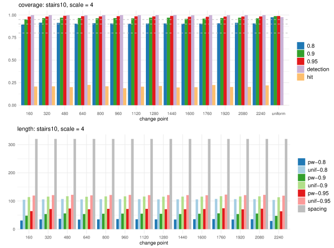
Figure 18: Bootstrap CIs constructed with model selection: stairs10 with $\vartheta=4$.

C.1.3 Comparison of coverage

Tables 4–5 compare the coverage of the bootstrap CIs constructed with the oracle estimators in (4) and those constructed with the model selection step, averaged over $2000$ realisations.

Table 4: Average coverage of the bootstrap CIs constructed with the oracle estimators and the estimators obtained from MoLP, when $\vartheta=1$. We also report the proportion of realisations where individual change points are detected (by MoLP) and where all change points are correctly detected.

test signal	$1-\alpha$	estimator	$\theta_{1}$	$\theta_{2}$	$\theta_{3}$	$\theta_{4}$	$\theta_{5}$	$\theta_{6}$	$\theta_{7}$	$\theta_{8}$	$\theta_{9}$	$\theta_{10}$	$\theta_{11}$	$\theta_{12}$	$\theta_{13}$	$\theta_{14}$	uniform
blocks	0.8	oracle	0.834	0.832	0.844	0.836	0.842	0.831	0.858	0.848	0.787	0.86	0.828	–	–	–	0.838
		MoLP	0.911	0.913	0.859	0.902	0.912	0.921	0.89	0.922	0.888	0.85	0.928	–	–	–	0.902
	0.9	oracle	0.921	0.915	0.932	0.926	0.912	0.912	0.954	0.922	0.892	0.941	0.914	–	–	–	0.926
		MoLP	0.96	0.965	0.92	0.95	0.964	0.965	0.95	0.974	0.937	0.913	0.97	–	–	–	0.932
	0.95	oracle	0.97	0.955	0.976	0.969	0.958	0.957	0.986	0.958	0.947	0.974	0.961	–	–	–	0.958
		MoLP	0.983	0.984	0.957	0.98	0.987	0.982	0.97	0.989	0.962	0.944	0.986	–	–	–	0.951
	—	detection	0.999	0.997	0.978	0.997	0.998	0.999	0.976	1	0.982	0.546	1	–	–	–	0.521
fms	0.8	oracle	0.891	0.887	0.968	0.875	0.87	0.859	–	–	–	–	–	–	–	–	0.856
		MoLP	0.852	0.93	0.992	0.815	0.833	0.919	–	–	–	–	–	–	–	–	0.908
	0.9	oracle	0.95	0.956	0.972	0.95	0.938	0.928	–	–	–	–	–	–	–	–	0.926
		MoLP	0.914	0.98	0.992	0.941	0.946	0.961	–	–	–	–	–	–	–	–	0.952
	0.95	oracle	0.974	0.978	0.986	0.978	0.969	0.972	–	–	–	–	–	–	–	–	0.962
		MoLP	0.945	0.993	0.996	0.979	0.981	0.98	–	–	–	–	–	–	–	–	0.966
	—	detection	0.928	1	1	0.964	0.986	1	–	–	–	–	–	–	–	–	0.895
mix	0.8	oracle	0.9	0.88	0.892	0.899	0.868	0.874	0.856	0.857	0.845	0.814	0.826	0.814	0.864	–	0.84
		MoLP	0.95	0.957	0.926	0.941	0.937	0.926	0.92	0.91	0.898	0.875	0.862	0.828	0.752	–	0.819
	0.9	oracle	0.956	0.948	0.95	0.946	0.926	0.938	0.922	0.926	0.928	0.908	0.934	0.922	0.942	–	0.927
		MoLP	0.964	0.981	0.972	0.971	0.974	0.969	0.965	0.964	0.953	0.931	0.93	0.894	0.857	–	0.888
	0.95	oracle	0.98	0.98	0.976	0.976	0.968	0.972	0.958	0.966	0.969	0.96	0.972	0.966	0.972	–	0.964
		MoLP	0.973	0.993	0.982	0.984	0.988	0.988	0.986	0.984	0.975	0.958	0.956	0.922	0.913	–	0.911
	—	detection	0.999	0.999	1	1	1	1	1	1	1	0.994	0.938	0.635	0.3	–	0.279
teeth10	0.8	oracle	0.878	0.874	0.868	0.872	0.876	0.876	0.872	0.868	0.88	0.856	0.863	0.864	0.862	–	0.784
		MoLP	0.894	0.977	0.983	0.982	0.985	0.989	0.981	0.976	0.98	0.983	0.982	0.981	0.905	–	0.889
	0.9	oracle	0.948	0.946	0.944	0.941	0.942	0.942	0.936	0.94	0.946	0.935	0.939	0.938	0.946	–	0.882
		MoLP	0.933	0.993	0.994	0.992	0.996	0.995	0.992	0.991	0.991	0.993	0.994	0.991	0.946	–	0.954
	0.95	oracle	0.976	0.976	0.974	0.976	0.972	0.974	0.974	0.971	0.971	0.976	0.974	0.974	0.972	–	0.939
		MoLP	0.958	0.996	0.997	0.997	0.998	0.996	0.996	0.996	0.997	0.997	0.997	0.995	0.975	–	0.979
	—	detection	0.962	0.946	0.948	0.952	0.952	0.951	0.951	0.954	0.953	0.951	0.948	0.952	0.964	–	0.7
stairs10	0.8	oracle	0.902	0.89	0.906	0.902	0.91	0.902	0.91	0.907	0.904	0.896	0.902	0.9	0.906	0.89	0.896
		MoLP	0.99	0.995	0.999	0.998	0.999	0.998	0.997	0.998	0.996	0.996	0.998	0.997	0.997	0.99	1
	0.9	oracle	0.956	0.96	0.966	0.967	0.967	0.964	0.96	0.964	0.964	0.96	0.968	0.962	0.97	0.958	0.962
		MoLP	0.997	0.998	0.999	0.999	0.999	0.999	0.999	0.999	0.998	0.998	0.999	0.998	0.999	0.995	1
	0.95	oracle	0.98	0.986	0.989	0.99	0.986	0.987	0.983	0.987	0.986	0.986	0.992	0.986	0.99	0.982	0.986
		MoLP	0.998	0.998	0.999	0.999	0.999	0.999	0.999	0.999	0.998	0.998	0.999	0.999	0.999	0.997	1
	—	detection	0.998	0.998	0.998	0.998	0.996	0.997	0.998	0.998	0.999	0.998	0.998	0.998	0.998	0.999	0.974

Table 5: Average coverage of the bootstrap CIs constructed with the oracle estimators and the estimators obtained from MoLP, when $\vartheta=4$. We also report the proportion of realisations where individual change points are detected (by MoLP) and where all change points are correctly detected.

test signal	$1-\alpha$	estimator	$\theta_{1}$	$\theta_{2}$	$\theta_{3}$	$\theta_{4}$	$\theta_{5}$	$\theta_{6}$	$\theta_{7}$	$\theta_{8}$	$\theta_{9}$	$\theta_{10}$	$\theta_{11}$	$\theta_{12}$	$\theta_{13}$	$\theta_{14}$	uniform
blocks	0.8	oracle	0.796	0.79	0.84	0.802	0.812	0.8	0.852	0.814	0.79	0.837	0.812	–	–	–	0.834
		MoLP	0.897	0.88	0.884	0.877	0.909	0.898	0.879	0.897	0.884	0.836	0.913	–	–	–	0.924
	0.9	oracle	0.895	0.902	0.938	0.903	0.905	0.894	0.957	0.908	0.899	0.93	0.9	–	–	–	0.911
		MoLP	0.956	0.953	0.941	0.947	0.962	0.962	0.945	0.956	0.943	0.92	0.965	–	–	–	0.94
	0.95	oracle	0.945	0.952	0.978	0.962	0.952	0.944	0.982	0.952	0.948	0.962	0.948	–	–	–	0.952
		MoLP	0.978	0.98	0.967	0.97	0.986	0.984	0.966	0.983	0.97	0.955	0.982	–	–	–	0.95
	—	detection	1	1	0.938	1	1	1	0.752	1	0.934	0.382	1	–	–	–	0.268
fms	0.8	oracle	0.877	0.812	0.83	0.82	0.796	0.813	–	–	–	–	–	–	–	–	0.846
		MoLP	0.79	0.872	0.918	0.85	0.874	0.88	–	–	–	–	–	–	–	–	0.796
	0.9	oracle	0.944	0.897	0.92	0.916	0.89	0.926	–	–	–	–	–	–	–	–	0.933
		MoLP	0.844	0.945	0.97	0.916	0.937	0.953	–	–	–	–	–	–	–	–	0.842
	0.95	oracle	0.971	0.947	0.963	0.968	0.946	0.972	–	–	–	–	–	–	–	–	0.966
		MoLP	0.865	0.974	0.988	0.954	0.966	0.976	–	–	–	–	–	–	–	–	0.858
	—	detection	0.438	1	1	0.974	0.977	0.992	–	–	–	–	–	–	–	–	0.426
mix	0.8	oracle	0.8	0.806	0.808	0.794	0.799	0.798	0.788	0.788	0.816	0.789	0.796	0.806	0.847	–	0.822
		MoLP	0.884	0.898	0.903	0.901	0.884	0.884	0.883	0.867	0.873	0.863	0.86	0.821	0.574	–	0.615
	0.9	oracle	0.906	0.904	0.905	0.9	0.898	0.908	0.898	0.895	0.911	0.9	0.922	0.918	0.935	–	0.917
		MoLP	0.948	0.959	0.96	0.961	0.945	0.952	0.946	0.942	0.938	0.933	0.919	0.883	0.672	–	0.692
	0.95	oracle	0.954	0.954	0.952	0.951	0.946	0.96	0.95	0.952	0.962	0.96	0.968	0.965	0.973	–	0.966
		MoLP	0.974	0.982	0.98	0.984	0.975	0.976	0.973	0.967	0.965	0.96	0.934	0.903	0.738	–	0.692
	—	detection	1	1	1	1	0.999	0.999	0.998	0.982	0.921	0.692	0.376	0.098	0.031	–	0.0065
teeth10	0.8	oracle	0.796	0.82	0.798	0.816	0.801	0.805	0.804	0.811	0.802	0.812	0.788	0.802	0.799	–	0.882
		MoLP	0.844	0.869	0.842	0.854	0.847	0.84	0.846	0.84	0.844	0.842	0.836	0.831	0.858	–	0.831
	0.9	oracle	0.904	0.928	0.916	0.927	0.916	0.916	0.926	0.923	0.919	0.92	0.918	0.922	0.908	–	0.964
		MoLP	0.923	0.933	0.928	0.929	0.926	0.912	0.929	0.924	0.925	0.919	0.914	0.92	0.921	–	0.91
	0.95	oracle	0.96	0.974	0.974	0.972	0.972	0.972	0.97	0.971	0.97	0.974	0.973	0.968	0.964	–	0.988
		MoLP	0.959	0.962	0.962	0.961	0.955	0.948	0.958	0.957	0.954	0.952	0.945	0.954	0.956	–	0.945
	—	detection	0.918	0.902	0.908	0.913	0.921	0.926	0.92	0.91	0.908	0.901	0.916	0.915	0.921	–	0.526
stairs10	0.8	oracle	0.814	0.822	0.82	0.828	0.818	0.814	0.82	0.833	0.826	0.83	0.816	0.826	0.83	0.823	0.926
		MoLP	0.893	0.915	0.913	0.904	0.909	0.906	0.903	0.907	0.906	0.904	0.905	0.908	0.913	0.907	0.975
	0.9	oracle	0.912	0.924	0.93	0.932	0.933	0.93	0.92	0.936	0.928	0.927	0.92	0.926	0.938	0.926	0.974
		MoLP	0.951	0.965	0.97	0.966	0.963	0.966	0.963	0.971	0.97	0.957	0.959	0.966	0.97	0.963	0.987
	0.95	oracle	0.962	0.972	0.976	0.979	0.976	0.97	0.974	0.974	0.967	0.97	0.97	0.975	0.974	0.967	0.987
		MoLP	0.981	0.982	0.991	0.986	0.984	0.986	0.985	0.984	0.99	0.98	0.979	0.982	0.983	0.984	0.989
	—	detection	0.998	0.998	0.998	0.996	0.998	0.998	0.998	1	1	0.996	0.998	0.997	0.998	0.998	0.976

C.2 $t_{5}$-distributed errors

C.2.1 Bootstrap CIs constructed with the oracle estimators in (4)

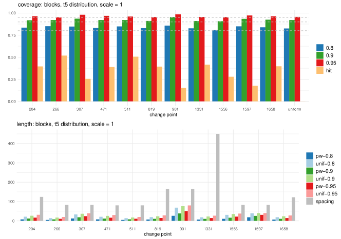
Figure 19: blocks with $\vartheta=1$.

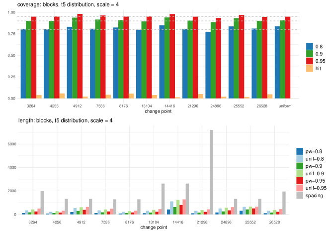
Figure 20: blocks with $\vartheta=4$.

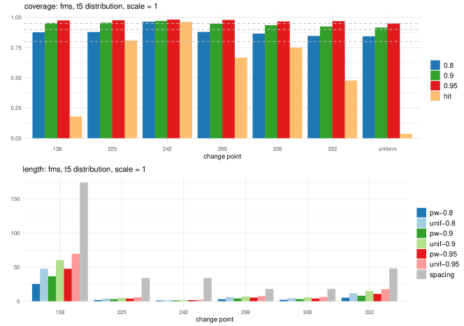
Figure 21: Bootstrap CIs constructed with the oracle estimators in (4): fms with $\vartheta=1$.

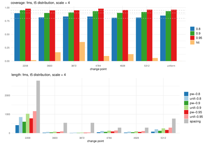
Figure 22: Bootstrap CIs constructed with the oracle estimators in (4): fms with $\vartheta=4$.

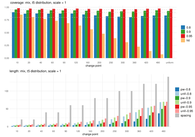
Figure 23: Bootstrap CIs constructed with the oracle estimators in (4): mix with $\vartheta=1$.

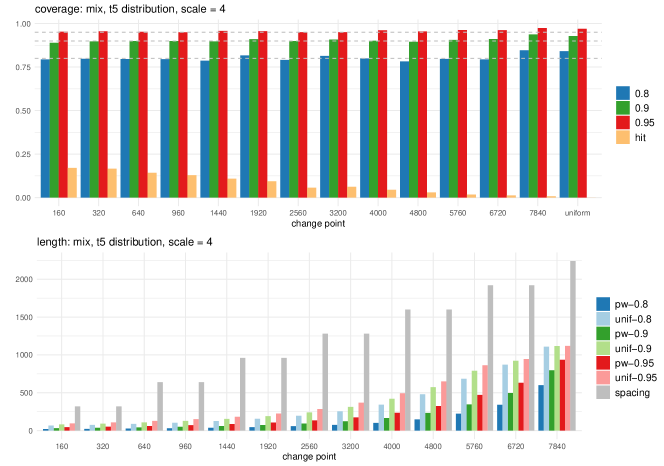
Figure 24: Bootstrap CIs constructed with the oracle estimators in (4): mix with $\vartheta=4$.

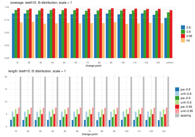
Figure 25: Bootstrap CIs constructed with theoracle estimators in (4): teeth10 with $\vartheta=1$.

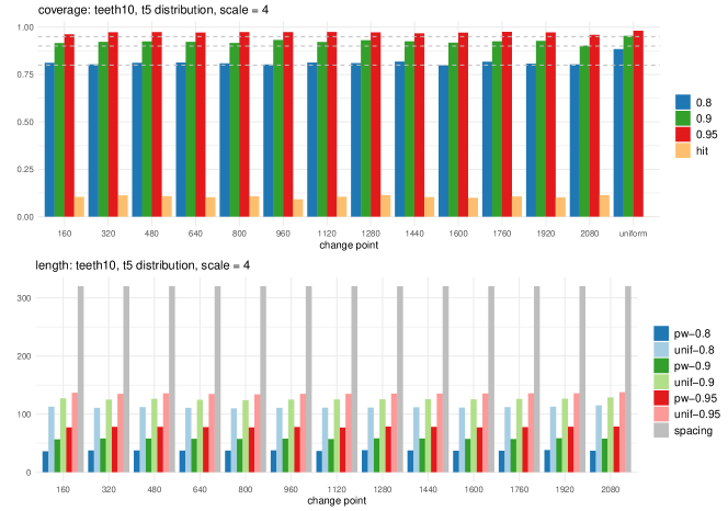
Figure 26: Bootstrap CIs constructed with the oracle estimators in (4): teeth10 with $\vartheta=4$.

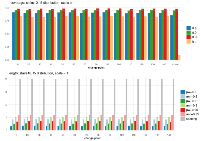
Figure 27: Bootstrap CIs constructed with the oracle estimators in (4): stairs10 with $\vartheta=1$.

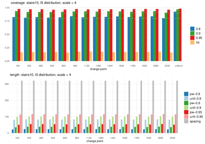
Figure 28: Bootstrap CIs constructed with the oracle estimators in (4): stairs10 with $\vartheta=4$.

C.2.2 Bootstrap CIs constructed with model selection

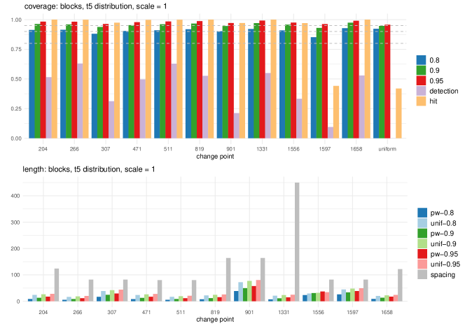
Figure 29: Bootstrap CIs constructed with model selection: blocks with $\vartheta=1$.

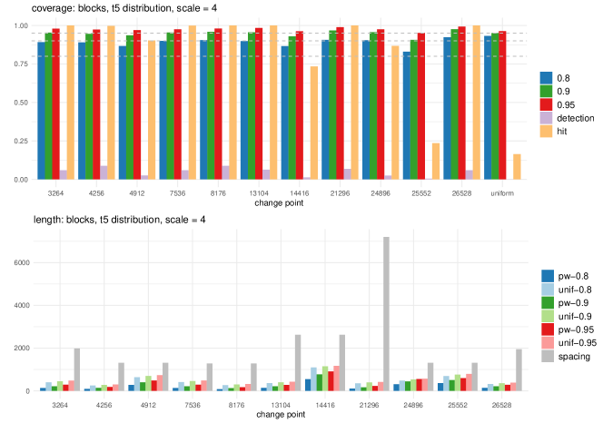
Figure 30: Bootstrap CIs constructed with model selection: blocks with $\vartheta=4$.

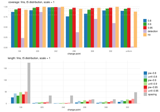
Figure 31: Bootstrap CIs constructed with model selection: fms with $\vartheta=1$.

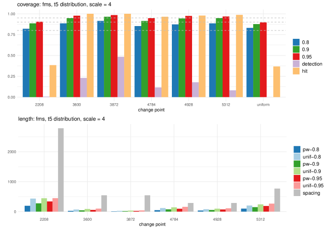
Figure 32: Bootstrap CIs constructed with model selection: fms with $\vartheta=4$.

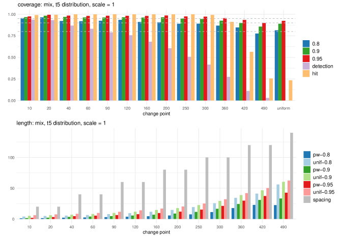
Figure 33: Bootstrap CIs constructed with model selection: mix with $\vartheta=1$.

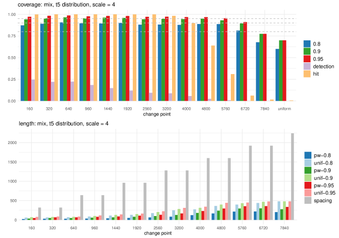
Figure 34: Bootstrap CIs constructed with model selection: mix with $\vartheta=4$.

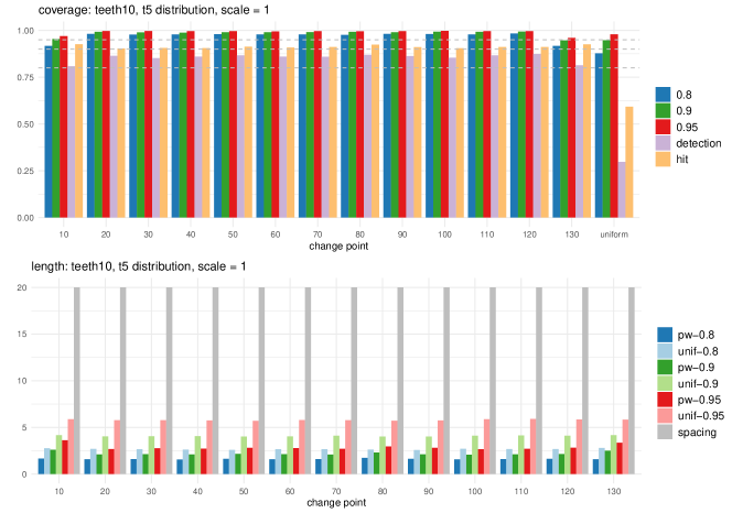
Figure 35: Bootstrap CIs constructed with model selection: teeth10 with $\vartheta=1$.

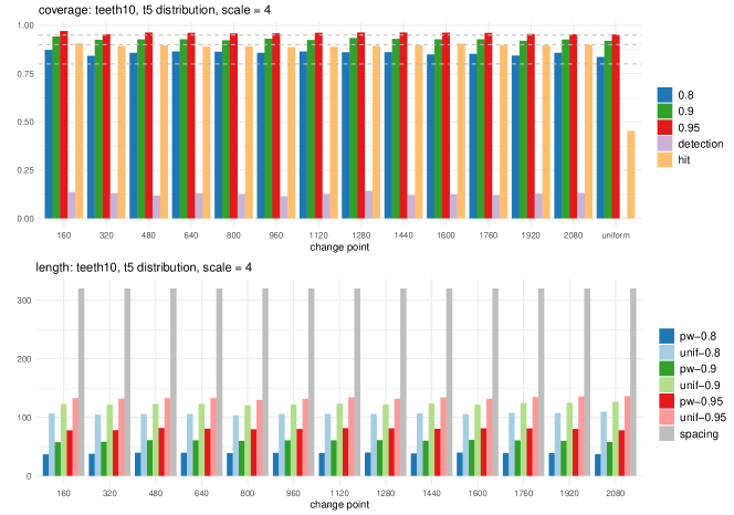
Figure 36: Bootstrap CIs constructed with model selection: teeth10 with $\vartheta=4$.

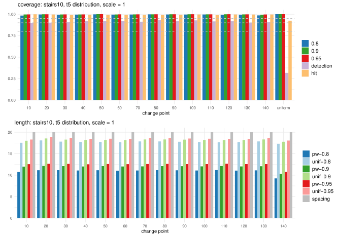
Figure 37: Bootstrap CIs constructed with model selection: stairs10 with $\vartheta=1$.

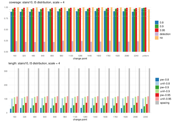
Figure 38: Bootstrap CIs constructed with model selection: stairs10 with $\vartheta=4$.

C.2.3 Comparison of coverage

Table 6: Average coverage of the bootstrap CIs constructed with the oracle estimators and the estimators obtained from MoLP, when $\vartheta=1$. We also report the proportion of realisations where individual change points are detected (by MoLP) and where all change points are correctly detected.

test signal	$1-\alpha$	estimator	$\theta_{1}$	$\theta_{2}$	$\theta_{3}$	$\theta_{4}$	$\theta_{5}$	$\theta_{6}$	$\theta_{7}$	$\theta_{8}$	$\theta_{9}$	$\theta_{10}$	$\theta_{11}$	$\theta_{12}$	$\theta_{13}$	$\theta_{14}$	uniform
blocks	0.8	oracle	0.835	0.851	0.847	0.831	0.848	0.828	0.858	0.826	0.81	0.849	0.838	–	–	–	0.826
		MoLP	0.913	0.914	0.88	0.904	0.91	0.919	0.903	0.922	0.909	0.851	0.928	–	–	–	0.923
	0.9	oracle	0.918	0.92	0.936	0.92	0.92	0.91	0.955	0.91	0.907	0.934	0.925	–	–	–	0.92
		MoLP	0.963	0.959	0.938	0.954	0.961	0.967	0.946	0.97	0.958	0.93	0.974	–	–	–	0.947
	0.95	oracle	0.964	0.952	0.98	0.968	0.96	0.955	0.985	0.956	0.954	0.973	0.963	–	–	–	0.956
		MoLP	0.983	0.982	0.963	0.979	0.984	0.988	0.971	0.992	0.975	0.963	0.99	–	–	–	0.957
	—	detection	1	0.999	0.974	0.998	0.999	1	0.971	1	0.97	0.441	1	–	–	–	0.419
fms	0.8	oracle	0.876	0.878	0.964	0.88	0.866	0.846	–	–	–	–	–	–	–	–	0.843
		MoLP	0.873	0.915	0.984	0.763	0.828	0.91	–	–	–	–	–	–	–	–	0.9
	0.9	oracle	0.954	0.956	0.97	0.948	0.935	0.924	–	–	–	–	–	–	–	–	0.916
		MoLP	0.933	0.974	0.986	0.936	0.927	0.956	–	–	–	–	–	–	–	–	0.95
	0.95	oracle	0.974	0.976	0.982	0.979	0.966	0.968	–	–	–	–	–	–	–	–	0.95
		MoLP	0.961	0.99	0.99	0.975	0.967	0.976	–	–	–	–	–	–	–	–	0.97
	—	detection	0.924	1	1	0.95	0.972	0.998	–	–	–	–	–	–	–	–	0.88
mix	0.8	oracle	0.904	0.873	0.878	0.874	0.876	0.876	0.858	0.84	0.823	0.814	0.806	0.828	0.838	–	0.838
		MoLP	0.955	0.964	0.922	0.919	0.924	0.935	0.91	0.907	0.89	0.891	0.868	0.848	0.777	–	0.814
	0.9	oracle	0.957	0.94	0.949	0.938	0.936	0.938	0.93	0.93	0.912	0.919	0.916	0.93	0.938	–	0.926
		MoLP	0.967	0.983	0.969	0.963	0.962	0.964	0.962	0.965	0.951	0.945	0.925	0.898	0.857	–	0.89
	0.95	oracle	0.98	0.973	0.97	0.968	0.972	0.973	0.966	0.968	0.963	0.962	0.962	0.97	0.972	–	0.968
		MoLP	0.975	0.994	0.984	0.98	0.983	0.982	0.98	0.986	0.975	0.973	0.955	0.934	0.898	–	0.924
	—	detection	0.991	0.994	1	1	1	1	1	1	1	0.992	0.912	0.564	0.256	–	0.234
teeth10	0.8	oracle	0.876	0.873	0.854	0.872	0.86	0.86	0.854	0.86	0.874	0.858	0.864	0.876	0.849	–	0.788
		MoLP	0.917	0.981	0.977	0.978	0.98	0.978	0.978	0.976	0.981	0.981	0.978	0.984	0.917	–	0.877
	0.9	oracle	0.942	0.941	0.934	0.941	0.938	0.939	0.928	0.934	0.946	0.934	0.934	0.936	0.928	–	0.896
		MoLP	0.954	0.992	0.99	0.988	0.99	0.99	0.991	0.992	0.99	0.993	0.992	0.993	0.947	–	0.947
	0.95	oracle	0.977	0.97	0.972	0.972	0.974	0.974	0.968	0.97	0.978	0.967	0.97	0.966	0.966	–	0.938
		MoLP	0.969	0.997	0.997	0.996	0.996	0.994	0.996	0.995	0.996	0.997	0.996	0.996	0.96	–	0.979
	—	detection	0.926	0.904	0.906	0.905	0.912	0.908	0.911	0.924	0.91	0.904	0.912	0.911	0.926	–	0.592
stairs10	0.8	oracle	0.909	0.892	0.899	0.892	0.906	0.907	0.89	0.904	0.91	0.9	0.89	0.897	0.894	0.898	0.854
		MoLP	0.983	0.996	0.993	0.995	0.998	0.995	0.995	0.997	0.996	0.995	0.996	0.993	0.994	0.986	1
	0.9	oracle	0.956	0.95	0.95	0.95	0.95	0.958	0.952	0.959	0.96	0.954	0.944	0.952	0.95	0.95	0.946
		MoLP	0.996	0.998	0.996	0.996	1	0.996	0.997	0.998	0.998	0.998	0.998	0.998	0.997	0.992	1
	0.95	oracle	0.979	0.978	0.98	0.978	0.982	0.982	0.977	0.984	0.984	0.982	0.976	0.98	0.982	0.98	0.976
		MoLP	0.997	0.998	0.997	0.997	1	0.998	0.997	0.998	0.998	0.999	0.998	0.999	0.998	0.996	1
	—	detection	0.998	0.996	0.992	0.994	0.993	0.993	0.992	0.991	0.994	0.996	0.989	0.996	0.996	0.996	0.924

Table 7: Average coverage of the bootstrap CIs constructed with the oracle estimators and the estimators obtained from MoLP, when $\vartheta=4$. We also report the proportion of realisations where individual change points are detected (by MoLP) and where all change points are correctly detected.

test signal	$1-\alpha$	estimator	$\theta_{1}$	$\theta_{2}$	$\theta_{3}$	$\theta_{4}$	$\theta_{5}$	$\theta_{6}$	$\theta_{7}$	$\theta_{8}$	$\theta_{9}$	$\theta_{10}$	$\theta_{11}$	$\theta_{12}$	$\theta_{13}$	$\theta_{14}$	uniform
blocks	0.8	oracle	0.808	0.806	0.831	0.809	0.824	0.797	0.85	0.808	0.774	0.836	0.811	–	–	–	0.838
		MoLP	0.892	0.89	0.867	0.9	0.905	0.898	0.866	0.906	0.904	0.83	0.923	–	–	–	0.933
	0.9	oracle	0.9	0.9	0.938	0.916	0.911	0.894	0.941	0.904	0.886	0.932	0.9	–	–	–	0.909
		MoLP	0.954	0.945	0.936	0.954	0.958	0.956	0.929	0.968	0.956	0.906	0.976	–	–	–	0.951
	0.95	oracle	0.95	0.952	0.981	0.964	0.951	0.952	0.98	0.949	0.934	0.969	0.946	–	–	–	0.949
		MoLP	0.98	0.973	0.97	0.975	0.98	0.984	0.963	0.989	0.975	0.951	0.992	–	–	–	0.963
	—	detection	1	0.997	0.903	0.999	1	1	0.734	1	0.867	0.235	1	–	–	–	0.164
fms	0.8	oracle	0.894	0.817	0.833	0.832	0.81	0.814	–	–	–	–	–	–	–	–	0.851
		MoLP	0.82	0.885	0.914	0.852	0.873	0.885	–	–	–	–	–	–	–	–	0.831
	0.9	oracle	0.953	0.899	0.91	0.932	0.903	0.917	–	–	–	–	–	–	–	–	0.932
		MoLP	0.885	0.947	0.964	0.913	0.944	0.947	–	–	–	–	–	–	–	–	0.876
	0.95	oracle	0.979	0.948	0.95	0.98	0.954	0.962	–	–	–	–	–	–	–	–	0.961
		MoLP	0.905	0.978	0.984	0.947	0.974	0.968	–	–	–	–	–	–	–	–	0.896
	—	detection	0.384	1	1	0.965	0.979	0.987	–	–	–	–	–	–	–	–	0.368
mix	0.8	oracle	0.794	0.797	0.796	0.795	0.786	0.817	0.791	0.814	0.8	0.782	0.796	0.794	0.846	–	0.841
		MoLP	0.873	0.891	0.907	0.896	0.894	0.901	0.88	0.882	0.878	0.888	0.887	0.813	0.677	–	0.6
	0.9	oracle	0.89	0.898	0.9	0.9	0.898	0.91	0.899	0.908	0.902	0.895	0.906	0.91	0.938	–	0.928
		MoLP	0.941	0.954	0.965	0.954	0.962	0.958	0.943	0.947	0.945	0.95	0.931	0.894	0.774	–	0.7
	0.95	oracle	0.954	0.955	0.952	0.95	0.958	0.956	0.95	0.95	0.961	0.954	0.962	0.962	0.974	–	0.97
		MoLP	0.972	0.983	0.986	0.978	0.982	0.98	0.971	0.973	0.968	0.968	0.955	0.911	0.774	–	0.7
	—	detection	0.998	1	1	1	1	1	0.999	0.982	0.899	0.64	0.31	0.062	0.016	–	0.005
teeth10	0.8	oracle	0.812	0.804	0.812	0.813	0.808	0.803	0.814	0.81	0.818	0.798	0.818	0.808	0.804	–	0.884
		MoLP	0.873	0.842	0.858	0.865	0.863	0.857	0.865	0.861	0.861	0.849	0.853	0.843	0.858	–	0.836
	0.9	oracle	0.916	0.922	0.924	0.922	0.916	0.932	0.922	0.931	0.926	0.918	0.926	0.928	0.903	–	0.954
		MoLP	0.942	0.925	0.927	0.928	0.923	0.931	0.924	0.934	0.93	0.928	0.928	0.92	0.927	–	0.92
	0.95	oracle	0.962	0.973	0.974	0.972	0.974	0.974	0.974	0.972	0.968	0.971	0.975	0.972	0.96	–	0.981
		MoLP	0.971	0.955	0.963	0.962	0.958	0.958	0.962	0.963	0.963	0.962	0.961	0.955	0.953	–	0.953
	—	detection	0.906	0.892	0.896	0.89	0.892	0.888	0.888	0.894	0.896	0.905	0.898	0.896	0.9	–	0.454
stairs10	0.8	oracle	0.824	0.813	0.823	0.814	0.82	0.839	0.82	0.83	0.829	0.836	0.824	0.834	0.838	0.804	0.925
		MoLP	0.901	0.898	0.9	0.901	0.909	0.911	0.917	0.911	0.914	0.917	0.921	0.913	0.912	0.9	0.977
	0.9	oracle	0.934	0.921	0.92	0.919	0.923	0.928	0.931	0.926	0.932	0.928	0.923	0.93	0.934	0.908	0.97
		MoLP	0.965	0.961	0.956	0.959	0.964	0.966	0.972	0.964	0.965	0.971	0.969	0.967	0.971	0.964	0.987
	0.95	oracle	0.976	0.971	0.971	0.962	0.968	0.974	0.968	0.974	0.97	0.972	0.975	0.976	0.976	0.963	0.982
		MoLP	0.987	0.987	0.979	0.978	0.984	0.987	0.987	0.981	0.984	0.986	0.986	0.982	0.986	0.981	0.993
	—	detection	0.998	0.997	0.996	0.993	0.998	0.994	0.995	0.998	0.997	0.998	0.998	0.995	0.998	0.996	0.952

C.3 Comparison with SMUCE

As noted in Section 5.2.3, SMUCE (Frick et al.,, 2014) returns confidence bands around change points at a prescribed level $\alpha$ which are readily comparable with the proposed uniform bootstrap CIs.

Several authors noted that the smaller $\alpha$ is set, the constraint imposed by SMUCE on the estimated residuals becomes more lenient and thus it tends to under-estimate the number of change points (Chen et al.,, 2014; Fryzlewicz, 2021a, ). This is demonstrated in Table 8 comparing MoLP (Cho and Kirch, 2021b , described in Section 5.2.2) and SMUCE with varying $\alpha\in\{0.1,0.2,0.45\}$ in terms of their detection accuracy. Here, the latter performs poorly in correctly detecting all $q_{n}$ change points compared to the former and in fact, with the exception of the fms test signal, attains this goal on far less than $10\%$ of realisations even when $\alpha$ is set as generously as $\alpha=0.45$.

Table 8: Proportion of the realisations (out of $2000$) where exactly $q_{n}$ change points estimators correctly detecting the change points are returned by MoLP (Cho and Kirch, 2021b, ) and SMUCE (Frick et al.,, 2014) applied with varying $\alpha\in\{0.1,0.2,0.45\}$ for the five test signals with $\vartheta=1$. We also provide in brackets the proportion of realisations where both MoLP and SMUCE at prescribed $\alpha$ detect all $q_{n}$ change points.

test signals	MoLP	SMUCE($0.45$)	SMUCE($0.2$)	SMUCE($0.1$)
blocks	0.480	0.0065	0.0005	0
	-	(0.0055)	(0)	(0)
fms	0.831	0.684	0.4215	0.248
	-	(0.5855)	(0.3665)	(0.2235)
mix	0.2595	0.0105	0.001	0
	-	(0.0085)	(0.001)	(0)
teeth10	0.698	0.0055	0.0005	0
	-	(0.0055)	(0.0005)	(0)
stairs10	0.9540	0.0785	0.011	0.002
	-	(0.075)	(0.011)	(0.002)

As inferential statements made by SMUCE about the locations of the change points is conditional on correctly estimating the number of change points, the lack of detection accuracy of SMUCE makes fair comparison between our proposed bootstrap methodology and SMUCE difficult. Figure 39 compares the uniform bootstrap CIs constructed with MoLP estimators and SMUCE CIs on the test signal fms. Here, both the coverage and the lengths of CIs are computed for each given confidence level only using the realisations where both MoLP and SMUCE correctly detect the all $q_{n}$ change points. In doing so, both uniform bootstrap CIs and SMUCE CIs show conservative coverage, while the latter are wider than the former at any given confidence level.

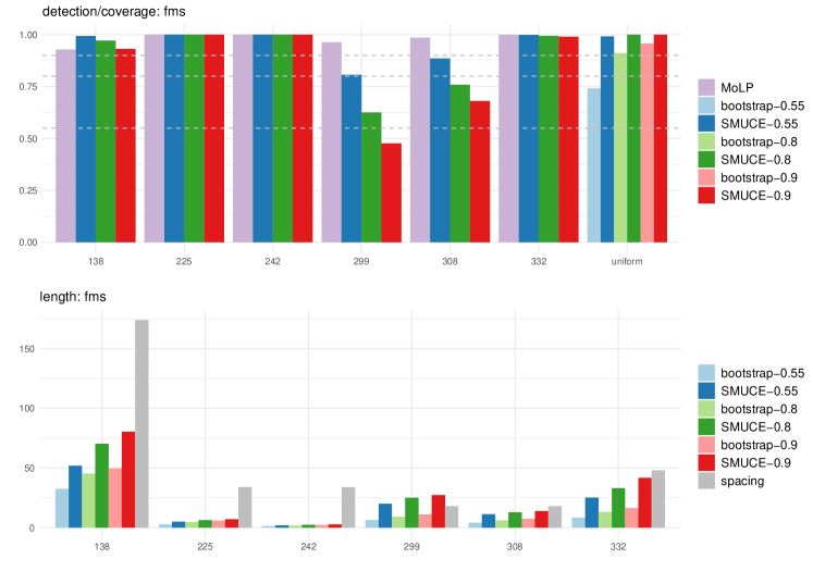
Figure 39: Comparison between Bootstrap CIs constructed with model selection and SMUCE: fms with $\vartheta=1$. Top: Proportion of correctly detecting each $\theta_{j}$ by MoLP and SMUCE (their locations given as the $x$-axis labels) and the coverage of the uniform bootstrap CIs constructed with the estimators from MoLP, and SMUCE CIs at varying confidence level $1-\alpha\in\{0.55,0.8,0.9\}$. Bottom: lengths of uniform bootstrap CIs and SMUCE CIs. We also report $2\delta_{j}$, twice the minimum distance to adjacent change points, for each $\theta_{j},\,j=1,\ldots,q_{n}$.

References

- Antoch and Hušková, (1999) Antoch, J. and Hušková, M. (1999). Estimators of changes. In Asymptotics, Nonparametrics, and Time Series, pages 557–561. CRC Press.
- Antoch and Hušková, (2001) Antoch, J. and Hušková, M. (2001). Permutation tests in change point analysis. Statistics & Probability Letters, 53(1):37–46.
- Antoch et al., (1995) Antoch, J., Hušková, M., and Veraverbeke, N. (1995). Change-point problem and bootstrap. Journal of Nonparametric Statistics, 5(2):123–144.
- Arias-Castro et al., (2018) Arias-Castro, E., Castro, R. M., Tánczos, E., and Wang, M. (2018). Distribution-free detection of structured anomalies: Permutation and rank-based scans. Journal of the American Statistical Association, 113(522):789–801.
- Bai and Perron, (1998) Bai, J. and Perron, P. (1998). Estimating and testing linear models with multiple structural changes. Econometrica, pages 47–78.
- Betken and Wendler, (2018) Betken, A. and Wendler, M. (2018). Subsampling for general statistics under long range dependence with application to change point analysis. Statistica Sinica, 28(3):1199–1224.
- Bücher and Kojadinovic, (2016) Bücher, A. and Kojadinovic, I. (2016). Dependent multiplier bootstraps for non-degenerate u-statistics under mixing conditions with applications. Journal of Statistical Planning and Inference, 170:83–105.
- Chen et al., (2014) Chen, Y., Shah, R. D., and Samworth, R. J. (2014). Discussion of Multiscale change point inference by Frick, Munk and Sieling. Journal of the Royal Statistical Society: Series B, 76:544–546.
- Cho and Fryzlewicz, (2020) Cho, H. and Fryzlewicz, P. (2020). Multiple change point detection under serial dependence: Wild constrast maximisation and gappy schwarz algorithm. arXiv preprint arXiv:2011.13884.
- (10) Cho, H. and Kirch, C. (2021a). Data segmentation algorithms: Univariate mean change and beyond. Econometrics and Statistics (to appear).
- (11) Cho, H. and Kirch, C. (2021b). Two-stage data segmentation permitting multiscale change points, heavy tails and dependence. Annals of the Institute of Statistical Mathematics (to appear).
- Dette et al., (2020) Dette, H., Schüler, T., and Vetter, M. (2020). Multiscale change point detection for dependent data. Scandinavian Journal of Statistics, 47:1243–1274.