A sparse approximate inverse for triangular matrices based on Jacobi iteration

Abstract

In this paper, we propose a simple sparse approximate inverse for triangular matrices (SAIT). Using the Jacobi iteration method, we obtain an expression of the exact inverse of triangular matrix, which is a finite series. The SAIT is constructed based on this series. We apply the SAIT matrices to iterative methods with ILU preconditioners. The two triangular solvers in the ILU preconditioning procedure are replaced by two matrix-vector multiplications, which can be fine-grained parallelized. We test this method by solving some linear systems and eigenvalue problems with preconditioned iterative methods.

Keywords: triangular solver, ILU factorization, iterative method, linear system, eigenvalue problem

1 Introduction

The incomplete LU (ILU) factorization is a type of general-purpose preconditioning techniques for sparse linear systems. There are two main problems in its parallelization. The first is the parallel generation of ILU factors. Many theories and techniques have been used to improve its parallelization. Here are some references on this problem [1, 3, 9, 14, 15, 18]. The second problem is solving triangular systems in the preconditioning procedure. It is easy to solve exactly a triangular system using forward or backward substitution method. However, this is a highly sequential process, and it may be executed many times in solving a system. This is an obstacle to exploit the performance of a parallel computing platform sufficiently. This is the main problem we shall study in this paper.

The simplest parallelization strategy in solving triangular systems is to compute the summations in the substitution methods in parallel:

$$\begin{split}x_{i}=\frac{1}{a_{ii}}\left(b_{i}-\sum_{k=1}^{i-1}a_{ik}x_{k}\right)\quad\text{or}\quad x_{i}=\frac{1}{a_{ii}}\left(b_{i}-\sum_{k=i+1}^{n}a_{ik}x_{k}\right).\end{split}$$

This is a low-level concurrent method, especially for sparse triangular matrices. Its corresponding blocking method can improve the performance. The level-scheduling method with reordering techniques improve the parallelism further [2]. These methods are exact solvers for triangular systems.

Another type of strategy is to replace the exact solutions of triangular systems by approximate ones. This ideal is based on the fact that the incomplete LU factorization is incomplete. This means that even the exact solutions of the triangular systems in ILU are not ’exact’ and these exact solutions could tolerate some errors. The Jacobi iteration method is an easy way to obtain approximate solutions [8, 9], and it mainly involves matrix-vector multiplications and vector additions, which are of fine-grained parallelism. An alternative method is to use sparse approximate inverses (SAI), which is based on the decay of inverses of sparse matrices [11, 12, 19]. With SAIs, the two triangular solvers in ILU preconditioning can be replaced by two matrix-vector multiplications. There are several ways to compute the SAI of a matrix, for example Frobenius norm minimization and incomplete inverse factorization [5, 6, 7, 20]. Also, there are some SAIs specially designed for triangular systems [4, 16, 22]. In [13, 21], the truncated Neumann expansions play a similar role to the SAIs of ILU factors. Some recent processes of this topic are introduced in [1].

When deriving the method we propose in this paper, we compress the Jacobi iteration method to a series firstly. As the iterative matrix in Jacobi iteration method for triangular systems is strictly triangular, the series is finite. We take the truncation of this series as the approximate inverse of triangular matrix and use some dropping strategies to make the inverse keep enough sparsity. We rewrite the truncation of the series as a recursive formula, by which we can avoid computing and storing high-order matrix powers. Then the SAIT algorithm is written in a quite brief way and it mainly involves sparse matrix-matrix multiplications and some dropping rules. The SAIT matrices can be applied to ILU preconditioning. The two triangular solvers can be replaced by two matrix-vector multiplications with a pair of SAIT matrices, which can be fine-grained parallelized.

This paper is organized as follows. In section 2, we propose an exact inverse for triangular matrices base on Jacobi iteration and then construct the general formulation of the SAIT algorithm. In section 3, we use two dropping strategies in the SAIT algorithm. In section 4, we take the SAIT matrices as preconditioners in solving linear systems and eigenvalue problems with preconditioned iterative methods. In section 5, there are some conclusions.

2 The basic idea of the SAIT algorithm

Let $T\in\mathbb{R}^{n\times n}$ be a triangular matrix. We solve the linear equation

$$\begin{split}Tx=b\end{split}$$

by Jacobi iteration method

$$\begin{split}x^{k}=D^{-1}(D-T)x^{k-1}+D^{-1}b.\end{split}$$ (1)

Here, $D$ is the diagonal matrix of $T$. For the sake of simplicity, we denote ${T}_{0}=I-D^{-1}T$. ${T}_{0}$ is a strictly triangular matrix. Then, (1) becomes

$$\begin{split}x^{k}={T}_{0}x^{k-1}+D^{-1}b.\end{split}$$

Letting the initial datum $x^{0}=0$, we list the solution of each iteration:

$$\begin{split}x^{1}&=D^{-1}b\\ x^{2}&={T}_{0}x^{1}+D^{-1}b=({T}_{0}+I)D^{-1}b\\ x^{3}&={T}_{0}x^{2}+D^{-1}b=({T}_{0}^{2}+{T}_{0}+I)D^{-1}b\\ &\cdots\\ x^{k}&={T}_{0}x^{k-1}+D^{-1}b=\left(\sum_{i=0}^{k-1}{T}_{0}^{i}D^{-1}\right)b.\\ \end{split}$$

Denoting

$$\begin{split}M_{k}=\sum_{i=0}^{k-1}{T}_{0}^{i}D^{-1},\end{split}$$ (2)

then we have

$$\begin{split}x^{k}=M_{k}b.\end{split}$$

As ${T}_{0}$ is a strictly triangular matrix, we have ${T}_{0}^{k}=0$ when $k\geq n$. Then we know that the exact inverse of $T$ is a finite series of (2), i.e.

$$\begin{split}T^{-1}=M_{n}\equiv\sum_{i=0}^{n-1}{T}_{0}^{i}D^{-1}.\end{split}$$ (3)

In the following, we construct approximate inverses for the triangular matrix $T$ based on its exact inverse (3). The approximation comes from two aspects, truncation and dropping. Let we study a truncated term $M_{m}$ of (3), where $m<n-1$ and

$$\begin{split}M_{m}=D^{-1}+{T}_{0}D^{-1}+{T}_{0}^{2}D^{-1}+\cdots+{T}_{0}^{m}D^{-1}.\end{split}$$ (4)

In order to avoid computing and storing the high-order terms ${T}_{0}^{i}$ $(i=1,\cdots,m)$ in (4), we rewrite $M_{k}$ as an equivalent form:

$$\begin{split}M_{0}D&=I,\\ M_{1}D&={T}_{0}+I,\\ M_{2}D&={T}_{0}({T}_{0}+I)+I,\\ M_{3}D&={T}_{0}({T}_{0}({T}_{0}+I)+I)+I,\\ &\cdots\\ \end{split}$$ (5)

This is the Horner’s method in calculating the values of polynomial functions. The same method was also proposed by a Chinese mathematician Qin Jiushao in $13^{th}$ century Song dynasty [23]. Furthermore, we present (5) in a recursive formula:

$$\begin{split}M_{0}D&=I,\\ M_{1}D&={T}_{0}(M_{0}D)+I,\\ M_{2}D&={T}_{0}(M_{1}D)+I,\\ M_{3}D&={T}_{0}(M_{2}D)+I,\\ &\cdots\\ M_{m}D&={T}_{0}(M_{m-1}D)+I.\\ \end{split}$$ (6)

To make the matrix more sparse, we perform dropping rules after each multiplication by ${T}_{0}$ in (6). This strategy is summarized in Algorithm 1.

Algorithm 1 Sparse Approximate Inverse for Triangular matrices base on Jacobi iteration (SAIT)

1:  Set the initial data $M=I$, let $D$ be the diagonal matrix of $T$ and let ${T}_{0}=I-D^{-1}T$.

2:  for  $k=1,2,\cdots,m$ do

3:     $M={T}_{0}M+I$

4:     execute dropping rules on $M$

5:  end for

6:  $M=MD^{-1}$

3 Dropping strategies

We use two dropping strategies, threshold-based and pattern-based, to concretize Algorithm 1.

Threshold-based. In step 3 of Algorithm 1, we drop the entries whose magnitudes are small than $\tau$ $(\tau<1)$ in $M$. As the diagonal entries of $M$ are all units, the setting $(\tau<1)$ can guarantee the matrix $M$ being always full-rank during the iterations. This strategy is presented in Algorithm 2. We paste the Matlab code for this algorithm in Appendix A.

Algorithm 2 Threshold-based Sparse Approximate Inverse for Triangular matrices SAIT_Thr$(\tau,m)$

1:  Set the initial data $M=I$, let $D$ be the diagonal matrix of $T$ and let ${T}_{0}=I-D^{-1}T$.

2:  for  $k=1,2,\cdots,m$ do

3:     $M={T}_{0}M+I$

4:     drop the entries in $M$ whose magnitudes are small than $\tau$ $(\tau<1)$

5:  end for

6:  $M=MD^{-1}$

Pattern-based. We set a fixed sparsity pattern ${\boldsymbol{S}}$ in advance, and drop the entries out of ${\boldsymbol{S}}$ in each iteration. The patterns of the power functions of the original matrix are often used in computing sparse approximate inverses [20]. We study the sparsity pattern of $T^{p}$ by

$$\begin{split}T^{p}=((T-D)+D)^{p}=\sum_{i=0}^{p}C_{p}^{i}D^{p-i}(T-D)^{i}.\end{split}$$

Since $(T-D)$ shares the same pattern with ${T}_{0}$, compared with (2), we know that $T^{p}$ has the same pattern with $M_{p+1}$. As $M_{p}$ tends to the exact inverse with $p\to n$, this pattern can be regarded as a truncated pattern of the exact inverse. When $p=0$, it is the Jacobi preconditioner, while when $p=1$, it is the pattern of the original matrix $T$. The pattern of $T^{p}$ can be obtained by Algorithm 1 without dropping any entries in the first $p$ iterations. Then, we keep the pattern of $T^{p}$, and in the following iterations, drop the entries out of this pattern. The number $p$ should not be too large, as the number of nonzeros in the pattern of $M_{p}$ increases rapidly with $p$ increasing. This dropping strategy is summarized in Algorithm 3.

Algorithm 3 Pattern-based Sparse Approximate Inverse for Triangular matrices SAIT_Pat$(p,m)$

1:  Set the initial data $M=I$, let $D$ be the diagonal matrix of $T$ and let ${T}_{0}=I-D^{-1}T$.

2:  for  $k=1,2,\cdots,p$ do

3:     $M={T}_{0}M+I$

4:  end for

5:  keep the sparsity pattern ${\boldsymbol{S}}$ of $M$

6:  for  $k=1,2,\cdots,m$ do

7:     $M={T}_{0}M+I$

8:     drop the entries in $M$ out of the pattern ${\boldsymbol{S}}$

9:  end for

10:  $M=MD^{-1}$

3.1 Balance between the accuracy and iteration counts

Let $L$ and $U$ be the two triangular factors of incomplete LU (ILU) factorization of a matrix $A$, and let $M_{L}$ and $M_{U}$ be the SAIT matrices for them respectively. In ILU preconditioning, the multiplication $LU$ can be regarded as an approximation of $A$, i.e. $LU\approx A$. If we take $M_{L}$ and $M_{U}$ as the approximations of $L^{-1}$ and $U^{-1}$, respectively, the multiplication $M_{U}M_{L}$ can be take an approximate inverse of $A$, i.e.

$$\begin{split}M_{U}M_{L}\approx U^{-1}L^{-1}\approx A^{-1}.\end{split}$$

When the ILU is taken as a preconditioner in an iterative method, we replace the two triangular equations $U(Lx)=y$ by two matrix-vector multiplications $x=M_{U}(M_{L}y)$.

In the Algorithm 2 and 3, if we use smaller threshold $\tau$ and larger $p$, we can obtain more accurate approximate inverses, since the SAIT matrices contains more nonzero entries. However, higher accuracy of SAIT matrices do not mean shorter runtime in solving a system with this preconditioner.

We list the following terms related to an iterative solver with the SAIT preconditioners:

• $iter(M_{L},M_{U})$: the iteration count of an iterative solver with $M_{L}$ and $M_{U}$ in preconditioning procedure.

• $comp(M_{L},M_{U})$: the runtime of computing the two matrix-vector multiplications $M_{U}(M_{L}y)$.

• $othercomp$: the runtime of computing other terms in each iteration except the preconditioning procedure.

Then, the runtime of a preconditioned iterative method can be estimated roughly by the following formula:

$$\begin{split}runtime=iter(M_{L},M_{U})\times\bigg{(}comp(M_{L},M_{U})+othercomp\bigg{)}.\end{split}$$ (7)

We define the ratios of a SAIT matrix $M_{T}$ compared with its original matrix $T$:

$$\begin{split}r=\frac{nnz(M_{T})}{nnz(T)},\end{split}$$

where $nnz(\cdot)$ denotes the number of nonzeros in a matrix. This value is to illustrate the number of nonzeros in a SAIT matrix, and it correlates to the runtime of the part $comp(M_{L},M_{U})$.

When we use iterative methods to solving a linear system, if the iterative method and the computer environment are fixed, the term $othercomp$ is usually fixed. If we use more accurate SAIT matrices, the iteration count $iter(M_{L},M_{U})$ decreases. However, we can not expect that the SAIT preconditioners can reduce the iteration count less than exact triangular solvers. It is probable that after exceeding some point, more nonzeros in $M_{L}$ and $M_{U}$ can not reduce the $iter(M_{L},M_{U})$ further. On the other side, more nonzeros can cause the term $comp(M_{L},M_{U})$ increasing, and sequentially, the total $runtime$ increasing.

In order to reduce the runtime, it should make a balance between the accuracy of SAIT matrices and the iteration count. As the accuracy is mainly decided by the threshold $\tau$ and the number $p$ in the Algorithm 2 and 3, respectively, there should be some $\tau$ or $p$ that make the runtime of an iterative solver with SAIT shortest. We call such parameters Optimal parameters. The optimal parameters may vary with different problems, different methods and different computer environments. We will verify the discussion above using numerical experiments in section 4.3.

4 Numerical experiments

In the numerical experiments, the main test models are the three-dimensional Laplace equation and its eigenvalue problem with homogeneous Dirichlet boundary condition:

$$\begin{split}-\Delta u&=f\quad\,\,\;\text{in}\,\,\Omega,\qquad u=0\quad\text{on}\,\,\partial\Omega\\ \text{and}\quad-\Delta u&=\lambda u\quad\text{in}\,\,\Omega,\qquad u=0\quad\text{on}\,\,\partial\Omega,\end{split}$$ (8)

where $\Omega=[0,1]^{3}$. We use a $102\times 102\times 102$ uniform mesh and finite difference method to discretize them. We obtain the corresponding matrix problems

$$\begin{split}Au_{h}&=f_{h}\\ \text{and}\quad Au_{h}&=\lambda_{h}u_{h}.\end{split}$$ (9)

Here, $A$ is a square matrix with $10^{6}$ rows/columns and it is symmetric positive definite (SPD). We use preconditioned conjugate gradient method (PCG) and LOBPCG method [17] to compute the linear equations and eigenvalue problem in (9), respectively.

We take the level-0 and level-1 ILU factors of the matrix $A$ as the original triangular systems and use the SAIT algorithms to approach their inverses. Then, we take the SAIT matrices as the preconditioners in PCG and LOBPCG. The SAIT matrices are generated by different SAIT algorithms with different parameters. We test and compare their effects in preconditioning the iterative solvers.

The code is implemented in Matlab and is run on a laptop with an Intel i7-6700HQ CPU with 16 GB RAM and a GTX970M GPU with 3 GB memory. We take $10^{-10}$ as the uniform stopping criteria for all the numerical experiments.

4.1 SAIT_Thr$(\tau,m)$ and SAIT_Pat$(p,m)$

We test the numbers of nonzeros in the SAIT matrices generated by the two dropping strategies, the SAIT_Thr$(\tau,m)$ in Algorithm 2 and SAIT_Pat$(p,m)$ in Algorithm 3. Figure 1 shows the ratios of nonzeros in SAIT matrices generated by SAIT_Thr$(\tau,m)$ with different threshold $\tau=0,\;0.01,\;0.02,\;0.05$ and increasing iteration number $m$. The setting $\tau=0$ means that there is no entry dropped in each iteration. In this case, the numbers of nonzeros increase rapidly. For other nonzero $\tau$, the numbers of nonzeros reach different stable states after several iterations. The smaller $\tau$ results in the more nonzeros in its corresponding SAIT matrix. For SAIT_Pat$(p,m)$, a fixed $p$ leads to a fixed pattern, which means that the number of nonzeros of its SAIT matrix is fixed. We put the ratios of the SAIT matrices generated by this algorithm in the legends of Figure 3.

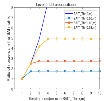
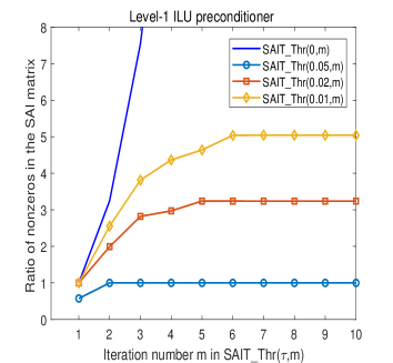
Figure 1: The ratios of the nonzeros in the SAIT matrices generated by SAIT_Thr$(\tau,m)$ with different $\tau$ and $m$ for level-0 (left) and level-1 (right) ILU factors.

Next, we test the effects of SAIT matrices as preconditioners in PCG method. For the matrices generated by SAIT_Thr$(\tau,m)$, the iteration counts of PCG decrease with increasing $m$ until reaching different stable states, shown in Figure 2. When using SAIT_Pat$(p,m)$, the iteration counts keep stable with $m$ varying, shown in Figure 3. For the both algorithms, the small threshold $\tau$ or larger $p$ (more nonzeros) means less iteration count. However, there is no case that the SAIT preconditioners can reduced the iteration counts less than the exact triangular solvers.

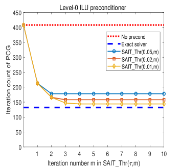
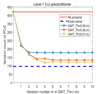
Figure 2: The iteration counts of PCG with SAIT preconditioners generated by SAIT_Thr$(\tau,m)$ with different $\tau$ and $m$ for level-0 (left) and level-1 (right) ILU factors.

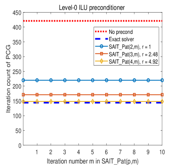
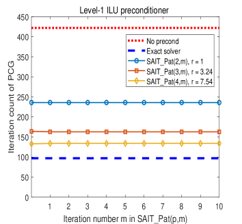
Figure 3: The iteration counts of PCG with SAIT preconditioners generated by SAIT_Pat$(p,m)$ with different $p$ and $m$ for level-0 (left) and level-1 (right) ILU factors.

We also compare the two dropping strategies with a fixed parameter $m=10$. As it is shown in Figure 4, with the same numbers of nonzeros, the PCG iteration counts of SAIT_Thr$(\tau,10)$ are less than that of SAIT_Pat$(p,10)$.

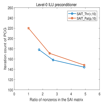
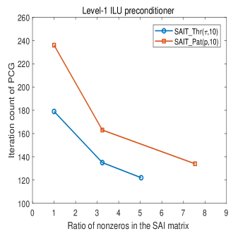
Figure 4: The comparisons of the iteration counts of PCG with SAIT preconditioner generated by SAIT_Thr$(\tau,m)$ and SAIT_Pat$(p,m)$ for level-0 (left) and level-1 (right) ILU factors.

4.2 The balance

Table 1 shows the iteration counts and runtime in solving the linear equation in (9) using PCG with the SAIT preconditioners. We observe that less iteration count does not means shorter runtime. We test more threshold parameters in SAIT_Thr$(\tau,m)$, shown in Figure 5. The iteration count does not decrease continuously with smaller threshold $\tau$ (more nonzeros) after some point. Even though we use the exact inverses which are usually full triangular matrices, the iteration count is equal to the exact triangular solver, which is not an arbitrarily small number. However, a SAIT matrix with too many nonzeros can increase the cost in computing matrix-vector multiplications. From the relation between the runtime and numbers of nonzeros, shown in the right picture of Figure 5, there should exists an optimal threshold $\tau$ in respect of the runtime. Such optimal parameter can be found by numerical experiments for each specific problem.

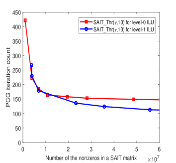
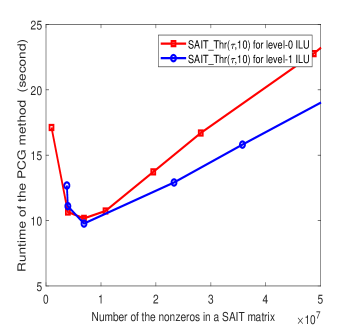
Figure 5: Left: the relation between the PCG iteration counts and the numbers of nonzeros in the SAIT preconditioners. Right:the relation between the runtime of PCG method and the numbers of nonzeros in the SAIT preconditioners.

4.3 Comparison with Jacobi iteration

Since the SAIT algorithms are designed based on Jacobi iteration method, if we use the Jacobi method in the preconditioning procedure directly, it is equivalent to the SAIT matrices generated by SAIT_Thr$(0,m)$, which are more accurate than the cases with thresholds $\tau>0$. In addition, it requires less memory, since a SAIT matrix usually has more nonzeros than its original matrix. We list the iteration counts and runtime of the Jacobi method in Table 2. The PCG iteration counts with Jacobi method can be almost the same as the exact solver after several iteration. However, its runtime is much longer than that of SAIT preconditioners in Table 1. The reason is that Jacobi method involves several matrix-vector multiplications and vector-vector additions in each PCG iteration, while there are only two matrix-vector multiplications with the SAIT preconditioners.

	level-0 ILU			level-1 ILU
	ratio	iter	time (s)	ratio	iter	time (s)
SAIT_Thr(0.05,10)	1.74	189	9.95	1.00	184	9.97
SAIT_Thr(0.02,10)	2.73	168	10.52	3.37	133	12.73
SAIT_Thr(0.01,10)	4.92	154	13.24	5.17	121	15.48
SAIT_Pat(1,10)	1.00	228	10.83	1.00	229	12.22
SAIT_Pat(2,10)	2.48	177	10.95	3.25	158	15.37
SAIT_Pat(3,10)	4.92	154	13.25	7.54	129	22.09

Table 1: The ratios the nonzeros, iteration count and runtime in solving the 3D FDM system using PCG method with different SAIT preconditoners. The red italic numbers are the least iteration account or the shortest runtime of the SAIT preconditoners generated by level-0 and level-1 ILU factors, respectively.

Jacobi iter	level-0 ILU		level-1 ILU
	iter	time (s)	iter	time (s)
1	423	29.88	423	31.87
2	229	21.03	240	24.78
3	173	19.33	169	22.10
4	152	20.43	134	21.19
5	152	23.23	116	21.48
6	149	25.94	108	23.45
7	147	28.19	104	24.74
8	146	30.76	101	27.21
9	145	33.67	97	28.38
10	145	36.60	98	31.31
11	145	39.53	98	33.90
12	145	42.28	98	36.50
13	145	45.66	98	39.25
14	145	48.44	97	41.43
15	145	51.54	97	47.38

Table 2: The iteration counts and runtime in solving the 3D FDM system in (9) using PCG method with Jacobi iteration method as preconditioner. The red italic numbers are the shortest runtime of level-0 and level-1 ILU factors, respectively.

4.4 Acceleration by GPU

The main computations of the basic Conjecture Gradient method are matrix-vector multiplications and vector-inner products. With the SAIT preconditioners, the preconditioning procedure are two matrix-vector multiplications. These operations can be highly parallelized. We use the function $gpuArray$ in Matlab to input the data into GPU. We run the solver with the same preconditioners in Table 1 on the GPU. Though the iteration counts are the similar with the experiments on CPU, the codes are accelerated several times by GPU, shown in Table 3.

	level-0 ILU			level-1 ILU
	ratio	iter	time (s)	ratio	iter	time (s)
SAIT_Thr(0.05,10)	1.74	189	1.34	1.00	184	1.34
SAIT_Thr(0.02,10)	2.73	168	1.33	3.37	133	1.59
SAIT_Thr(0.01,10)	4.92	154	1.81	5.17	121	1.81
SAIT_Pat(1,10)	1.00	228	1.47	1.00	229	1.67
SAIT_Pat(2,10)	2.48	177	1.36	3.25	158	1.92
SAIT_Pat(3,10)	4.92	154	1.80	7.54	129	2.38

Table 3: The same codes in Table 1 are run on GPU.

4.5 Preconditioned solver for eigenvalue problems

When we use the simultaneous preconditioned method LOBPCG to compute the eigenvalue problem in (9), there are many vectors to be dealt with in the preconditioning procedure of each iteration. With SAIT preconditioners, this procedure can be done through two matrix-matrix multiplications. Here, we use the LOBPCG method to compute the first 4 eigenvalues in this problems. We use level-0 and level-1 ILU factorizations, and use SAIT_Thr$(0.01,10)$ to generated the SAIT matrices. Figure 6 and 7 show their results, respectively.

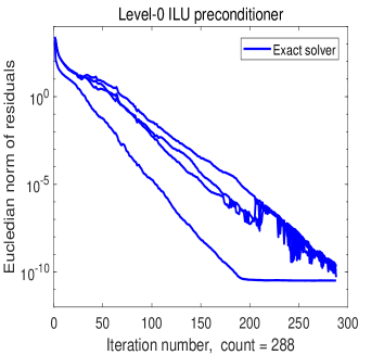
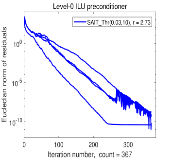
Figure 6: The convergence history in solving Laplace eigenvalue problem using LOPBCG method with the exact solver and a SAT preconditioner generate by SAIT_Thr$(0.03,10)$ for level-0 ILU factors in the preconditioning procedure.

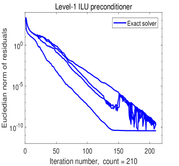
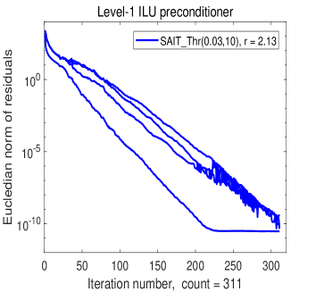
Figure 7: The convergence history in solving Laplace eigenvalue problem using LOPBCG method with the exact solver and a SAT preconditioner generated by SAIT_Thr$(0.03,10)$ for level-1 ILU factors in the preconditioning procedure.

4.6 More examples

We apply the SAIT algorithms to more examples, shown in Table 4. These examples are from the University of Florida sparse matrix collection [10]. Table 5 are the results using the SAIT_Thr$(\tau,10)$ preconditioners. Here, the ratios of nonzeros in the SAIT matrices generated by their corresponding thresholds (may be not optimal) are mainly between 1 and 2. We also try SAIT_Pat$(p,10)$ for these examples, shown in Table 6. Comparing with the results in the two tables, we find that the threshold-based SAIT_Thr$(\tau,10)$ preconditioners preform better than the pattern-based SAIT_Pat$(p,10)$ for these problems. In Table 5, we also compare the iteration counts of SAIT preconditioners with the exact solver. Even though more iterations, the runtime of SAIT can be reduced by parallelization as it is discussed in section 4.4.

	row/column	nnz
apache1	80800	542184
apache2	715176	4817870
thermal1	82654	574458
thermal2	1228045	8580313
parabolic_fem	525825	3674625
G3_circuit	1585478	7660826
ecology2	999999	4995991
thermomech_dM	204316	1423116
thermomech_TC	102158	711558

Table 4: The numbers of rows and nonzeros of some SPD matrices in [10].

	no p.c.	level-0 ILU					level-1 ILU
		exact	$\tau$	ratio	SAIT		exact	$\tau$	ratio	SAIT
apache1	3777	365	0.05	1.46	439	20.3%	249	0.03	1.80	316	26.9%
apache2	5528	882	0.05	1.39	1092	23.8%	587	0.03	1.70	797	35.8%
thermal1	1707	651	0.05	1.43	703	8.0%	363	0.04	1.76	435	19.8%
thermal2	6626	2555	0.05	1.42	2763	8.1%	1401	0.04	1.72	1674	19.5%
parabolic_fem	3515	1423	0.1	0.96	1640	15.2%	845	0.04	1.32	946	12.0%
thermomech_dM	89	10	0.06	1.01	11	10.0%	6	0.02	1.02	8	33.3%
thermomech_TC	89	10	0.06	1.01	11	10.0%	6	0.02	1.02	8	33.3%
ecology2	7127	2123	0.08	2.00	2830	33.3%	1303	0.06	3.25	1942	49.0%
G3_circuit	21205	1182	0.08	2.07	1582	33.8%	643	0.08	2.38	1174	82.6%

Table 5: The iteration counts of PCG method with the exact solver and SAIT preconditioners generated by SAIT_Thr$(\tau,10)$.

	level-0 ILU				level-1 ILU
	m = 2		m = 3		m = 2		m = 3
	ratio	SAIT	ratio	SAIT	ratio	SAIT	ratio	SAIT
thermomech_dM	1	11	1.60	10	1	10	2.37	6
thermomech_TC	1	11	1.60	10	1	10	2.37	6
thermal1	1	847	1.85	690	1	743	2.49	440
thermal2	1	3284	1.85	2674	1	2868	2.48	1635
parabolic_fem	1	1678	1.56	1451	1	1444	2.38	893
apache1	1	3252	2.41	2236	1	4102	3.11	2570
apache2	1	2753	2.42	1818	1	3521	3.12	2500
G3_circuit	1	3993	2.04	2751	1	3713	2.37	2245
ecology2	1	3738	2.00	2799	1	3765	2.25	2549

Table 6: The iteration counts of PCG method with the SAIT preconditioners generated by SAIT_Pat$(p,10)$.

5 Conclusion

We derive an exact inverse for triangular matrix trough Jacobi iteration method. The inverse is a finite series. We take the truncation of this series as the approximate inverse for a triangular matrix. To make the approximate inverses more sparse, we propose two dropping strategies. We apply the SAIT matrices to iterative method with ILU preconditioners. Then the two triangular solvers in ILU preconditioning are replaced by two matrix-vector multiplications, which can be fine-grained parallelized. We present some numerical examples to show the effects of SAIT preconditioners. Though the iteration counts of SAIT matrices are larger than the exact triangular solvers, the runtime can be reduced by parallelization. In this paper, we only present the basic study on this method. There are many things about this method are remained to be studied further, for example, more efficient dropping strategies, choices of the parameters and parallel implementations.

Appendix A The Matlab code of SAIT_Thr$(\tau,m)$

⬇

function M = SAIT_Thr(T,tau,m)

I = speye(size(T,1));

Dn = diag(diag(T).^(-1));

T0 = I - Dn*T;

M = I;

for i = 1 : m

M = T0*M + I;

P = (abs(M)>tau);

M = M.*P;

end

M = M*Dn;

end

References

- [1] Ahmad Abdelfattah, Hartwig Anzt, Jack Dongarra, Mark Gates, Azzam Haidar, Jakub Kurzak, Piotr Luszczek, Stanimire Tomov, Ichitaro Yamazaki, and Asim YarKhan. Linear algebra software for large-scale accelerated multicore computing. Acta Numerica, 25:1–160, 2016.
- [2] Edward Anderson and Youcef Saad. Solving sparse triangular linear systems on parallel computers. Internat. J. High Speed Comput., 1(01):73–95, 1989.
- [3] Hartwig Anzt, Edmond Chow, and Jack Dongarra. ParILUT—a new parallel threshold ILU factorization. SIAM J. Sci. Comput., 40(4):C503–C519, 2018.
- [4] Hartwig Anzt, Thomas K. Huckle, Jürgen Bräckle, and Jack Dongarra. Incomplete sparse approximate inverses for parallel preconditioning. Parallel Comput., 71:1–22, 2018.
- [5] Michele Benzi. Preconditioning techniques for large linear systems: a survey. J. Comput. Phys., 182(2):418–477, 2002.
- [6] Michele Benzi, Carl D. Meyer, and Miroslav Tůma. A sparse approximate inverse preconditioner for the conjugate gradient method. SIAM J. Sci. Comput., 17(5):1135–1149, 1996.
- [7] Michele Benzi and Miroslav Tuma. A comparative study of sparse approximate inverse preconditioners. Appl. Numer. Math., 30(2-3):305–340, 1999.
- [8] Edmond Chow, Hartwig Anzt, Jennifer Scott, and Jack Dongarra. Using Jacobi iterations and blocking for solving sparse triangular systems in incomplete factorization preconditioning. J. Parallel Distrib. Comput., 119:219–230, 2018.
- [9] Edmond Chow and Aftab Patel. Fine-grained parallel incomplete LU factorization. SIAM J. Sci. Comput., 37(2):C169–C193, 2015.
- [10] Timothy A. Davis and Yifan Hu. The University of Florida sparse matrix collection. ACM T. Math. Software (TOMS), 38(1):1, 2011.
- [11] Stephen Demko, William F. Moss, and Philip W Smith. Decay rates for inverses of band matrices. Math. Comp., 43(168):491–499, 1984.
- [12] Victor Eijkhout and Ben Polman. Decay rates of inverses of banded M-matrices that are near to toeplitz matrices. Linear Algebra Appl., 109:247–277, 1988.
- [13] Ivar Gustafsson and Gunhild Lindskog. Completely parallelizable preconditioning methods. Numer. Linear Algebra Appl., 2(5):447–465, 1995.
- [14] Pascal Hénon and Yousef Saad. A parallel multistage ILU factorization based on a hierarchical graph decomposition. SIAM J. Sci. Comput., 28(6):2266–2293, 2006.
- [15] David Hysom and Alex Pothen. A scalable parallel algorithm for incomplete factor preconditioning. SIAM J. Sci. Comput., 22(6):2194–2215, 2001.
- [16] Carlo Janna, Massimilano Ferronato, and Giuseppe Gambolati. A block FSAI-ILU parallel preconditioner for symmetric positive definite linear systems. SIAM J. Sci. Comput., 32(5):2468–2484, 2010.
- [17] Andrew V. Knyazev. Toward the optimal preconditioned eigensolver: Locally optimal block preconditioned conjugate gradient method. SIAM Journal on Scientific Computing, 23(2):517–541, 2001.
- [18] Mardochée Magolu monga Made and Henk A. van der Vorst. A generalized domain decomposition paradigm for parallel incomplete LU factorization preconditionings. Future Gener. Comp. Sy., 17(8):925–932, 2001.
- [19] Reinhard Nabben. Decay rates of the inverse of nonsymmetric tridiagonal and band matrices. SIAM J. Matrix Anal. Appl., 20(3):820–837, 1999.
- [20] Yousef Saad. Iterative methods for sparse linear systems, volume 82. SIAM, 2003.
- [21] Henk A. van der Vorst. A vectorizable variant of some ICCG methods. SIAM J. Sci. Statist. Comput., 3(3):350–356, 1982.
- [22] Arno C. N. van Duin. Scalable parallel preconditioning with the sparse approximate inverse of triangular matrices. SIAM J. Matrix Anal. Appl., 20(4):987–1006, 1999.
- [23] Wen-tsun Wu. Grand Series of Chinese Mathematics (in Chinese), volume V. Beijing Normal University Publishing House, 2000.