Combining Astrometry and Elemental Abundances: The Case of the Candidate Pre-Gaia Halo Moving Groups G03-37, G18-39, and G21-22

Abstract

While most moving groups are young and nearby, a small number have been identified in the Galactic halo. Understanding the origin and evolution of these groups is an important piece of reconstructing the formation history of the halo. Here we report on our analysis of three putative halo moving groups: G03-37, G18-39, and G21-22. Based on Gaia EDR3 data, the stars associated with each group show some scatter in velocity (e.g., Toomre diagram) and integrals of motion (energy, angular momentum) spaces, counter to expectations of moving-group stars. We choose the best candidate of the three groups, G21-22, for follow-up chemical analysis based on high-resolution spectroscopy of six presumptive members. Using a new Python code that uses a Bayesian method to self-consistently propagate uncertainties from stellar atmosphere solutions in calculating individual abundances and spectral synthesis, we derive the abundances of $\alpha$- (Mg, Si, Ca, Ti), Fe-peak (Cr, Sc, Mn, Fe, Ni), odd-$Z$ (Na, Al, V), and neutron-capture (Ba, Eu) elements for each star. We find that the G21-22 stars are not chemically homogeneous. Based on the kinematic analysis for all three groups and the chemical analysis for G21-22, we conclude the three are not genuine moving groups. The case for G21-22 demonstrates the benefit of combining kinematic and chemical information in identifying conatal populations when either alone may be insufficient. Comparing the integrals of motion and velocities of the six G21-22 stars with those of known structures in the halo, we tentatively associate them with the Gaia-Enceladus accretion event.

1 Introduction

The advent of imaging and spectroscopic all-sky surveys over the past two decades has enabled great advances in the study of Milky Way stellar populations and led to the realization that our Galaxy is teeming with substructure (e.g., Helmi, 2020). Notable examples include the Sagittarius dwarf galaxy (e.g., Ibata et al., 1994; Lynden-Bell & Lynden-Bell, 1995; Newberg et al., 2002; Majewski et al., 2003), the dozens of other dwarf galaxies that surround the Milky Way (e.g., Willman et al., 2005), the remnants of the Gaia-Enceladus/Sausage major merger $\approx$10 Gyr ago (Belokurov et al., 2018; Helmi et al., 2018), and other dynamically tagged groups (e.g., Yuan et al., 2020; Naidu et al., 2020; Limberg et al., 2021). Today, thanks to data produced from the ground and from space by e.g., the Dark Energy Survey (Dark Energy Survey Collaboration et al., 2016), the Zwicky Transient Facility (Bellm et al., 2019), Gaia (Gaia Collaboration et al., 2018a) and TESS (Ricker et al., 2015), we are gaining ever deeper understanding of our Galaxy.

Table 1: Literature Properties of G03-37, G18-39, and G21-22

		$U^{\prime}$			$V^{\prime}$			$\left(U^{\prime 2}+W^{\prime 2}\right)^{1/2}$			[Fe/H]			$V_{\mathrm{rot}}$
		(km s-1)			(km s-1)			(km s-1)						(km s-1)
Groups		min	max		min	max		min	max		min	max		min	max
G03-37		-60	55		-335	-255		42	100		-1.79	-1.00		-88	-19
G18-39		-250	-165		-316	-225		162	250		-1.79	-1.00		-88	-19
G21-22		210	287		-316	-202		162	278		-1.79	-1.00		-88	-19

Note. — The data are the range of values characteristic of each candidate group given in Silva et al. (2012). $U^{\prime}$, $V^{\prime}$, and $W^{\prime}$ velocities were derived using radial velocities and proper motions from multiple literature sources and the matrix equations of Johnson & Soderblom (1987), and corrected for the Sun’s velocity $(U,V,W)_{\odot}=(+10.0,+14.9,+7.7)~{}\mathrm{km~{}s}^{-1}$. [Fe/H] were determined using new and literature Strömgren photometry and the calibration equations of Schuster et al. (2006), and $V_{\mathrm{rot}}=V^{\prime}+220~{}\mathrm{km~{}s}^{-1}$, where $220~{}\mathrm{km~{}s}^{-1}$ was taken as the velocity of the local standard of rest about the Galactic center.

For instance, it is now generally accepted that the Galactic halo is composed of two stellar populations, characterized by the blue and red sequences of the Gaia Herztsprung-Russell diagram (Gaia Collaboration et al., 2018a). Stars on the blue sequence tend to be relatively metal-poor, more deficient in $\alpha$-elements (O, Mg, S, Si, Ca, Ti), and have kinematics that are consistent with an accreted population. By contrast, stars on the red sequence are relatively more metal-rich, have more enhanced $\alpha$-element abundances, and have kinematics suggesting these stars formed in situ, either in the disk and subsequently dynamically heated to halo-type orbits, or in the halo itself (e.g., Carollo et al., 2007; Nissen & Schuster, 2010, 2011; Schuster et al., 2012; Ramírez et al., 2012; Haywood et al., 2018; Hawkins et al., 2015).

Identifying halo stars that formed in situ is critical to fully elucidating the evolution of the Galaxy. Here, we examine three halo moving groups from Silva et al. (2012), who identified seven new halo moving groups tentatively associated with $\omega$ Cen and the Kapteyn moving group. We note that the Kapteyn moving group had been long hypothesized to be tidal debris from $\omega$ Cen (e.g. Wylie-de Boer et al., 2010), but this was proven to be unlikely by means similar to the present work (Navarrete et al., 2015). Silva et al. (2012) identified their moving groups using a combination of Strögren photometry of 142 metal-poor stars obtained at the Observatorio Astronómico Nacional at San Pedro Mártir in Baja California, Mexico, and photometry, radial velocities, and proper motions of additional stars from multiple literature sources. Using well established calibrations, they determined distances, metallicities (i.e., [Fe/H]), absolute magnitudes ($M_{\mathrm{V}}$), and Galactic space velocities corrected for the Sun’s velocity ($U^{\prime}$, $V^{\prime}$, $W^{\prime}$) for a total of 1695 stars.

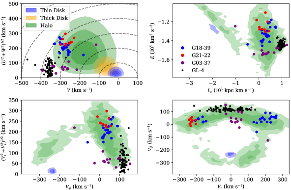
Figure 1: We compare the stars in our three moving groups to stars from the thin disk (blue contours), thick disk (orange contours), halo (green contours), and from the halo substructure GL-4 (Li et al., 2019), for different kinematic metrics describing their motion around the Galaxy. The top left panel shows a Toomre diagram (the contours in this panel show synthetic stars, while all other panels show stars from Gaia DR2 that are kinematically selected as being part of either the thin disk or halo), $\left(U^{2}+W^{2}\right)^{1/2}$ vs. $V$, comparing the stars’ Galactic space velocities. The other panels compare $E$ vs. $L_{\mathrm{z}}$, the orbital energy against the azimuthal angular momentum (top right), $(V^{2}_{\mathrm{r}}+V^{2}_{\mathrm{z}})^{1/2}$ vs. $V_{\phi}$, the combined radial and longitudinal velocities against the azimuthal velocity around the Galaxy (bottom left), and $V_{\phi}$ vs. $V_{\mathrm{r}}$, the azimuthal velocity against the radial velocity. While none of the three Silva et al. (2012) moving groups is as tightly clustered as are the members of GL-4, the stars in G21-22 do appear relatively clustered, suggesting it is the most likely bona fide moving group of the three.

We report our first application of a two-pronged approach to validating stellar associations, Gaia astrometry and chemical abundance analysis, i.e., chemical tagging. We adopted as a starting point the definition of a moving group from (Eggen, 1958), which associates stars based on common space motions. This implies that the stars share a common orbital path about the Galactic center and have done so for at least some amount of time in the past. We further constrained this idea to include the notion that the stars have a shared formation history, i.e., they formed from the same molecular cloud at about the same time. In this scenario, the stars were once members of a now dissociated open cluster or other conatal stellar association and thus, in addition to their shared kinematics, they should have the same age and composition. In addition to this definition, other possible interpretations of moving groups exist, including stars trapped in dynamical resonances arising from the bar or spiral arms (e.g., Amarante et al., 2020) or accreted stars from dwarf galaxies (e.g., Haywood et al., 2018), both sets of which could share common space motions but not necessarily formation histories.

We started with three putative halo moving groups identified by Silva et al. (2012) and for which we had high-resolution spectroscopy: G03-37, G18-39, and G21-22. As is the case with all the groups in Silva et al. (2012), the authors named these moving groups after candidate member stars that appear in the Lowell Proper Motions Survey (Giclas et al., 1959, 1961, 1975). In the sections that follow, we describe our use of precise Gaia proper motions and parallaxes, as well as Gaia radial velocities, to investigate the kinematic properties and dynamical histories of the stars in each group. We then describe our detailed chemical abundance analysis of six stars in G21-22, which we identify as the best candidate to constitute a coherent moving group. Our analysis relied on our new abundance derivation code that uses Bayesian and Markov chain Monte Carlo (MCMC) methods to self-consistently derive stellar parameters, abundances, and uncertainties. We conclude the paper with a discussion on the validity of the G03-38, G18-39, and G21-22 moving groups, and the potential origin of the G21-22 stars.

2 Gaia Astrometry

We first analyzed the dynamical characteristics of the stars in the three moving groups from Silva et al. (2012) on which we focus. A summary of the properties of these groups as presented by Silva et al. (2012) is given in Table 1. We found that nine G03-38, 15 G18-39, and six G21-22 stars have counterparts in the early third Gaia data release (EDR3; Gaia Collaboration et al., 2021; Lindegren et al., 2021) with measured radial velocities. For these stars we have complete six-dimensional phase space information (see Table 7), allowing us to fully analyze the kinematics of the stars in these groups. All kinematic quantities have been derived using the Galactic modeling framework of Astropy v4.0 (Astropy Collaboration et al., 2013, 2018) and the Galactic modeling code, gala (Price-Whelan, 2017), with its built-in Galactic potential MilkyWayPotential (see Table 8). This model combines the disk model from Bovy (2015) with a spherical NFW profile (Navarro et al., 1997).

In the top left panel of Figure 1, we show a Toomre diagram of the stars in each moving group, plotting their combined $(U^{2}+W^{2})^{1/2}$ velocity against $V$. By comparing the positions of the stars in the three Silva et al. (2012) moving groups to those of the Milky Way thin disk, thick disk, and halo populations defined in Bensby et al. (2003), we concluded that the stars in each of the three groups are indeed consistent with being members of the Milky Way halo.

In the remaining three panels, we compare the stars’ integrals of motion, i.e., orbital energy, $E$, against their azimuthal angular momentum, $L_{\mathrm{z}}$ (top right), the azimuthal velocity, $V_{\phi}$, around the Galaxy against the combined radial, $V_{\mathrm{r}}$, and longitudinal, $V_{\mathrm{z}}$, velocities (bottom left), and $V_{\phi}$ against $V_{\mathrm{r}}$ (bottom right). Background contours in each of the three panels represent a random selection of Gaia EDR3 stars with measured radial velocities; halo stars (green contours) are defined by having $(U^{2}+V^{2}+W^{2})^{1/2}>$ 300 km s^-1, while thin disk stars (blue contours) are defined as having $(U^{2}+V^{2}+W^{2})^{1/2}<$ 25 km s^-1. In all four panels of Figure 1, we also compare the three halo moving groups to GL-4, a halo substructure identified in Gaia and LAMOST data by Li et al. (2019).

Regardless of which kinematic parameters are being used, the stars in each of the three Silva et al. (2012) groups show significant scatter—more than is observed within GL-4—calling into question their designation as a moving group. Of the three groups, G21-22 (red symbols) shows the least scatter.

We also used gala and its Galactic potential MilkyWayPotential to integrate stellar orbits around the Milky Way. We defined each star’s position in phase space using its astrometric parameters (position, proper motion, and parallax; Lindegren et al., 2021) and Gaia EDR3 radial velocity (measured by Gaia’s Radial Velocity Spectrometer; Cropper et al., 2018), then integrated each stars’ position backward in time for 200 Myr.

Figure 2 shows that the stars in each of these moving groups do not follow kinematically coherent orbits. Even for G21-22, the Silva et al. (2012) moving group we identified in Figure 1 as having the least scatter, the stellar orbits diverge (see the bottom two panels of Figure 2). This orbital inconsistency strongly suggests that these three moving groups are actually spurious stellar associations. However, uncertainties in the measurement of astrometric parameters, particularly in the parallax, or details of the Galactic model can lead to inaccurate orbits. Therefore, to further constrain the nature of these putative moving groups, we selected the best candidate, G21-22, for a detailed abundance analysis.

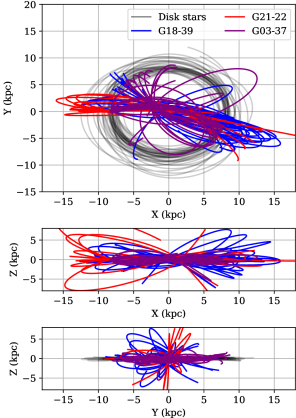
Figure 2: We integrate the orbit of stars (colored lines) in each of the three stellar groups in a Milky Way potential backwards in time for 200 Myr. Compared to randomly chosen disk stars (black lines) the stars in each of the three stellar groups exhibit halo-like orbits. At the accuracy afforded by Gaia EDR3 astrometric precision and radial velocity measurements, none of these three groups appear to have a common origin.

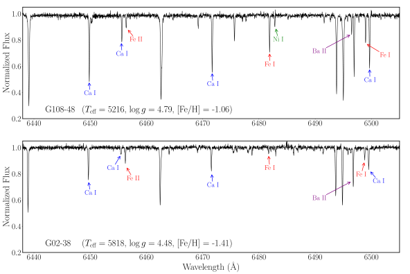
Figure 3: Sample VLT/UVES spectra of G108-48 (top) and G02-38 (bottom), two putative members of G21-22. Some of the lines that have been measured are indicated.

3 Chemical Compositions

3.1 Observations and Data Reduction

We obtained high-resolution spectroscopy of six stars identified by Silva et al. (2012) as members of G21-22 in service mode with the Ultraviolet and Visual Echelle Spectrograph (UVES; Dekker et al., 2000) and the 8.2-m Unit 2 (UT2, Kueyen) telescope of the Very Large Telescope (VLT) at Cerro Paranal, Chile, between the months of 2012 October and 2013 March. A standard dichroic setting (DIC 1) was used to provide a wavelength (incomplete) coverage of 3280 to 6800 Å. The slit width was set to $0.6^{\prime\prime}$, giving a nominal resolving power of $R\approx 65,000$, and the Poisson signal-to-noise (S/N) of the spectra is $\approx$100 near 6500 Å. The data were reduced through the observatory’s standard pipeline processing using the REFLEX environment (Freudling et al., 2013) within the European Southern Observatory Common Pipeline Library and were taken directly from the ESO Science Archive. Representative samples of the spectra are shown in Figure 3.

3.2 Equivalent Widths

We derived stellar parameters and abundances of up to 13 elements—Na, Mg, Al, Si, Ca, Sc, Ti, V, Cr, Mn, Fe, Ni, and Ba—via an equivalent width (EW) analysis assuming local thermodynamic equilibrium (LTE) line formation for each star. Starting with the spectral lines analyzed by Villanova & Geisler (2011) and Sakari et al. (2019), we constructed our linelist with those falling in the wavelength coverage of our VLT/UVES spectra. The transition probabilities ($\log gf$) were checked against atomic parameters based on recent accurate laboratory data provided by the Wisconsin atomic physics program (e.g., Yousefi & Bernath, 2018; Lawler et al., 2019). The laboratory data were accessed via the Python tool Linemake, developed by Vinicius Placco (Placco et al., 2021). In all cases of discrepancy, the laboratory transition probabilities were adopted. The linelist is provided in Table 2.

Table 2: Linelist and Equivalent Widths for Putative Members of G21-22

		$\lambda$		$\chi$		$\log gf$		Equivalent Widths
Species		(Å)		(eV)				G02-38		G82-42	G108-48	119-64	G161-73	HIP 36878
Na I		5682.63	2.10	-0.70	$\cdots$	$\cdots$	19.8	$\cdots$	11.0	21.9
		5688.21	2.10	-0.45	$\cdots$	24.6	33.3	10.1	19.2	31.5
		6160.75	2.10	-1.26	$\cdots$	$\cdots$	6.9	$\cdots$	$\cdots$	$\cdots$
Mg I		5528.41	4.34	-0.62	$\cdots$	169.3	$\cdots$	80.8	121.2	$\cdots$
		5711.09	4.34	-1.83	32.1	58.5	$\cdots$	15.8	35.3	65.7
		6318.72	5.10	-1.73	$\cdots$	$\cdots$	9.3	$\cdots$	$\cdots$	$\cdots$
		6319.24	5.10	-1.95	7.4	$\cdots$	5.5	$\cdots$	$\cdots$	$\cdots$
Al I		6696.02	3.14	-1.35	$\cdots$	$\cdots$	7.2	$\cdots$	$\cdots$	3.7
Si I		5684.52	4.93	-1.65	9.3	14.0	13.9	$\cdots$	12.0	$\cdots$
		5701.10	4.93	-2.05	$\cdots$	$\cdots$	$\cdots$	$\cdots$	$\cdots$	9.2

Note. — Table 2 is published in its entirety online in the machine-readable format. A portion is shown here for guidance regarding its form and content.

EWs of each line were measured using the Python tool pyEW, developed by Monika Adamów. The code attempts to fit each spectral line from a user-provided linelist with Gaussian, multiple Gaussian (combined), and Voigt profiles and provides the best fit as the one that minimizes the least squares errors in the fit to the observed line. All lines were inspected visually to ensure the goodness of each fit. The EWs of each measured line are included in Table 2.

3.3 Stellar Parameters, Abundances, and Errors

To derive stellar parameters and abundances, we made use of our newly developed Python code, SPAE (Stellar Parameters, Abundances, and Errors), that uses a state-of-the-art Bayesian method to self-consistently propagate uncertainties from the stellar atmosphere solutions in calculating individual abundances. SPAE employs the LTE plane-parallel spectral analysis code MOOG (MOOGSILENT version; Sneden, 1973) and Kurucz (2011) model atmosphere grids to derive the abundances of elements included in a user-provided linelist. We note that in the following and throughout the paper, we distinguish [Fe/H]_m, the metallicity of a star relative to the Sun, and [Fe/H], the Fe abundance of a star relative to the solar Fe abundance. The former is used as an input for a model atmosphere; the latter is an output of MOOG.

Starting with an (adjustable) initial parameter grid step defined by an effective temperature ($T_{\rm eff}$), surface gravity ($\log g$), metallicity ([Fe/H]_m), and microturbulent velocity ($\xi$), the code interpolates the Kurucz grids to produce a model atmosphere, and then passes the model and linelist to MOOG to derive the abundances. The resulting Fe I and Fe II abundances are read by SPAE and used to construct the likelihood function, $\mathcal{L}$, which is defined by the minimization of the differences in the derived [Fe I/H] and [Fe II/H] abundances and the model metallicity, [Fe/H]_m:

$$\ln\mathcal{L}_{\mathrm{Fe\,I}}=-N_{\mathrm{Fe\,I}}\times\ln\sigma_{\mathrm{Fe}}+\sum-\frac{\left([\mathrm{Fe\,I/H}]-[\mathrm{Fe/H}]_{\mathrm{m}}\right)^{2}}{2\sigma_{\mathrm{Fe}}^{2}}$$ (1)

and

$$\ln\mathcal{L}_{\mathrm{Fe\,II}}=-N_{\mathrm{Fe\,II}}\times\ln\sigma_{\mathrm{Fe}}+\sum-\frac{\left([\mathrm{Fe\,II/H}]-[\mathrm{Fe/H}]_{\mathrm{m}}\right)^{2}}{2\sigma_{\mathrm{Fe}}^{2}},$$ (2)

where $\sigma_{\mathrm{Fe}}$ is the standard deviation of the combined line-by-line abundances of [Fe I/H] and [Fe II/H], and $N_{\mathrm{Fe\,I}}$ and $N_{\mathrm{Fe\,II}}$ are the number of Fe I and Fe II lines, respectively. The log of the likelihood function is then the sum of the two separate log-likelihoods in Equations 1 and 2:

$$\ln\mathcal{L}=\ln\mathcal{L}_{\mathrm{Fe\,I}}+\ln\mathcal{L}_{\mathrm{Fe\,II}}.$$

Table 3: Stellar Parameters for the Putative G21-22 Members

		G02-38		G82-42		G108-48		G119-64		G161-73		HIP 36878
$T_{\rm eff}$ (K)		$5818\,^{\,+43}_{-\,42}$		$5413\,^{+\,42}_{-\,43}$		$5212\,^{+\,46}_{-\,47}$		$6149\pm 50$		$5981\,^{+\,36}_{-\,33}$		$5333\;^{+\,32}_{-\,34}$
$\log g$ (cgs)		$4.48\pm 0.08$		$4.61\pm 0.08$		$4.77\,^{+\,0.11}_{-\,0.10}$		$4.06\,^{+\,0.12}_{-\,0.13}$		$3.97\,^{+\,0.08}_{-\,0.09}$		$4.55\pm 0.05$
$\xi$ (km s-1)		$1.27\pm 0.08$		$0.65\,^{+\,0.13}_{-\,0.18}$		$0.78\,^{+\,0.18}_{-\,0.21}$		$1.54\pm 0.06$		$1.45\pm 0.05$		$0.49\,^{+\,0.13}_{-\,0.18}$
$\mathrm{[Fe/H]}_{\mathrm{m}}$		$-1.41\pm 0.03$		$-1.17\pm 0.04$		$-1.07\pm 0.04$		$-1.56\pm 0.04$		$-1.07\pm 0.03$		$-1.13\pm 0.03$
Iterations		26,600		30,420		31,200		28,000		30,000		34,000

Table 4: Abundances of Putative G21-22 Stars

		G02-38		G82-42		G108-48		G119-64		G161-73		HIP 36878
$\mathrm{[Fe\;I/H]}$		$-1.41\;\pm 0.03$		$-1.17\;\pm 0.04$		$-1.07\;\pm 0.04$		$-1.56\;\pm 0.04$		$-1.07\;\pm 0.03$		$-1.13\;\pm 0.03$
$\mathrm{[Fe\;II/H]}$		$-1.41\;\pm 0.04$		$-1.19\;\pm 0.05$		$-1.07\;\pm 0.05$		$-1.56\;\pm 0.05$		$-1.06\;\pm 0.04$		$-1.13\;\pm 0.03$
$\mathrm{[Na/Fe]}$		$\cdots$		$-0.36\;\pm 0.05$		$-0.36\;\pm 0.05$		$0.00\;\pm 0.04$		$-0.24\;\pm 0.05$		$-0.20\;\pm 0.04$
$\mathrm{[Mg/Fe]}$		$0.45\;\pm 0.04$		$0.18\;\pm 0.11$		$-0.23\;\pm 0.05$		$0.31\;\pm 0.04$		$0.29\;\pm 0.08$		$0.39\;\pm 0.03$
$\mathrm{[Al/Fe]}$		$\cdots$		$\cdots$		$-0.24\;\pm 0.05$		$\cdots$		$\cdots$		$-0.40\;\pm 0.03$
$\mathrm{[Si/Fe]}$		$0.35\;\pm 0.07$		$0.14\;\pm 0.05$		$0.07\;\pm 0.04$		$\cdots$		$0.19\;\pm 0.09$		$-0.05\;\pm 0.17$
$\mathrm{[Ca/Fe]}$		$0.17\;\pm 0.05$		$0.18\;\pm 0.06$		$0.07\;\pm 0.06$		$0.31\;\pm 0.06$		$0.21\;\pm 0.05$		$0.13\;\pm 0.05$
$\mathrm{[Sc/Fe]}$		$0.13\;\pm 0.06$		$0.11\;\pm 0.09$		$0.12\;\pm 0.08$		$0.12\;\pm 0.08$		$0.02\;\pm 0.06$		$0.16\;\pm 0.06$
$\mathrm{[Ti\;I/Fe]}$		$0.19\;\pm 0.05$		$0.23\;\pm 0.06$		$0.20\;\pm 0.07$		$0.34\;\pm 0.06$		$0.15\;\pm 0.06$		$0.18\;\pm 0.05$
$\mathrm{[Ti\;II/Fe]}$		$0.31\;\pm 0.05$		$0.17\;\pm 0.08$		$0.22\;\pm 0.07$		$0.36\;\pm 0.07$		$0.19\;\pm 0.06$		$0.33\;\pm 0.05$
$\mathrm{[V/Fe]}$		$\cdots$		$0.03\;\pm 0.10$		$0.11\;\pm 0.08$		$\cdots$		$\cdots$		$-0.01\;\pm 0.05$
$\mathrm{[Cr/Fe]}$		$-0.17\;\pm 0.06$		$0.02\;\pm 0.09$		$0.02\;\pm 0.07$		$-0.09\;\pm 0.09$		$-0.18\;\pm 0.05$		$-0.03\;\pm 0.05$
$\mathrm{[Mn/Fe]}$		$-0.41\;\pm 0.08$		$-0.41\;\pm 0.09$		$-0.29\;\pm 0.06$		$-0.44\;\pm 0.05$		$-0.33\;\pm 0.05$		$-0.34\;\pm 0.06$
$\mathrm{[Ni/Fe]}$		$-0.03\;\pm 0.05$		$-0.10\;\pm 0.06$		$-0.08\;\pm 0.06$		$-0.09\;\pm 0.06$		$-0.16\;\pm 0.05$		$-0.07\;\pm 0.04$
$\mathrm{[Ba/Fe]}$		$-0.03\;\pm 0.07$		$\cdots$		$0.23\;\pm 0.10$		$-0.04\;\pm 0.08$		$0.02\;\pm 0.07$		$0.37\;\pm 0.06$

The parameter space is sampled using emcee (Foreman-Mackey et al., 2013), a Python implementation of an affine-invariant ensemble sampler Markov-Chain Monte Carlo (MCMC) algorithm (Goodman & Weare, 2010). We adopted a four-dimensional– $T_{\rm eff}$, $\log g$, [Fe/H]_m, and $\xi$– flat prior probability distribution constrained by the available Kurucz model atmosphere grids. The ensemble solution (posterior probability distribution) is generated by initializing 40 walkers in an $N$-ball around Solar values ($T_{\rm eff}$$=$5777 K, $\log g$$=$4.44, [Fe/H]_m$=$0.01, $\xi$$=$1.38 km s^-1), then iterating 1000 steps, resulting in $4\times 10^{4}$ separate combinations of parameters that are used to produce model atmospheres that are passed onto MOOG to derive abundances.

Figure 4: Fe I abundance versus excitation potential ($\chi$; top) and reduced equivalent width ($\log\mathrm{RW}$; bottom) for the median solution for G161-73. The black line is the least squares fit to the data, with the $r$-value (correlation coefficient) and $p$-value (Wald test with t-distribution) shown in the lower left.

The derived $T_{\rm eff}$, $\log g$, [Fe/H]_m, $\xi$, elemental abundances, and their uncertainties are taken as the median and $1\sigma$ confidence intervals of the ensemble solutions, after accounting for burn-in (iterations to convergence, typically 200-300) and any walkers with low acceptance fractions ($<$$0.40$). We calculated autocorrelation lengths with built-in functions in emcee, and they were found to be $\lesssim 100$ for each star. Note that [Fe/H]_m is determined by considering both Fe I and Fe II, as defined by $\mathcal{L}$. The parameters, along with the final number of iterations included in the ensemble solutions, are given for each star in Table 3.

In addition to the stellar parameters and metallicity, the abundances of the other elements measured are derived with each iteration of the MCMC, resulting in ensemble solutions for each element. In Table 4, the medians and $1\sigma$ confidence intervals of the ensemble solutions for each element are shown, with the abundances given relative to the solar values of Asplund et al. (2009) .

The implementation in SPAE of the likelihood function $\mathcal{L}$ is a departure from the typical method used to spectroscopically derive stellar parameters and abundances. The more typical method, excitation and ionization balance of Fe I and Fe II, entails requiring the line-by-line Fe I abundances to be independent of excitation potential ($\chi$) and EW, and requiring the mean [Fe/H] abundances as derived from Fe I and Fe II lines to be the same. The uncertainties are then typically determined by altering the stellar parameters to achieve $1\sigma$ deviations in the correlations between $\chi$, EW, and the Fe I abundances (e.g., Schuler et al., 2011).

While ionization balance is intrinsic to $\mathcal{L}$, excitation balance is not. Therefore, the ability to check the excitation balance of the median solution, as well as identifying any solution(s) in the ensemble that achieve excitation balance, has been built into SPAE. This allows the user to verify that the solution(s) obtained using the typical method is contained in the posterior distribution and determine its (their) statistical significance relative to the distribution.

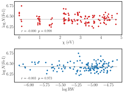
Figure 5: Fe I abundance versus excitation potential (top) and reduced equivalent width (bottom) for the solution satisfying excitation balance at the highest confidence level for G161-73. The black line is the least squares fit to the data, with the $r$-value and $p$-value shown in the lower left.

As an example, in Figure 4 we show the plots of $\log_{10}N$(Fe I) as a function of $\chi$ and reduced equivalent width ($\log_{10}\mathrm{RW}$) for the median solution for G161-73. A linear least squares fit is applied to each relation. For $\chi$, the $r$-value (correlation coefficient) is $r=-0.037$ and the corresponding $p$-value (Wald test with t-distribution) is $p=0.663$, and for $\log_{10}\mathrm{RW}$, $r=-0.009$ and $p=0.916$. While the statistical significance of $r$ is marginal for $\log_{10}\mathrm{RW}$, the $p$-value for $\chi$ indicates that the data are not consistent with the null hypothesis of having a slope of zero and thus formally do not satisfy excitation balance, the criteria for which we have adopted to be $\lvert r\rvert<0.01$ and $p>0.90$. However, of the 30,000 iterations included in the ensemble solution for G161-73, 17 of them do satisfy excitation balance. In Figure 5 we show the correlation plots for the solution satisfying excitation balance at the highest confidence level for G161-73. With $r=-0.000$ and $p=0.998$ for $\chi$ and $r=-0.003$ and $p=0.973$ for $\log_{10}\mathrm{RW}$, this solution is consistent with both relations having a slope of zero. The differences in $T_{\rm eff}$, $\log g$, [Fe/H]_m, and $\xi$ between this solution and the median solution are $-9$ K, $-0.07$ dex, $-0.01$ dex, and 0.02 km $s^{-1}$, respectively.

The position of this solution is indicated by the blue lines in Figure 6, which summarizes the ensemble solution for the stellar parameters of G161-72 as determined by SPAE. All four parameters are within $1\sigma$ of those of the median solution, indicating that SPAE is able to converge on the correct solution for this star. A direct comparison of the SPAE solutions to the solutions satisfying excitation balance at the highest confidence level for each star is shown in Figure 7.

The mean of the stellar parameters of the solutions satisfying excitation balance for each star is provided in Table 5; standard deviations and the number of solutions are also given. The standard deviations demonstrate that although numerous solutions satisfy excitation balance for each star, those solutions occupy a tight parameter space, as would be expected. A major advantage of SPAE is that these solutions are contained in the generated ensemble solution and therefore taken into account in the final stellar parameter and abundance uncertainties. Indeed, the $1\sigma$ confidence intervals of the ensemble solutions are a true measure of the uncertainty in the parameters and abundances as derived with our data.

Table 5: Excitation Balance Stellar Parameters of Putative G21-22 Stars

		G02-38		G82-42		G108-48		G119-64		G161-73		HIP 36878
$T_{\rm eff}$ (K)		$5804.0\pm 1.8$		$5415.4\pm 3.8$		$5197.4\pm 3.9$		$6130.3\pm 1.3$		$5970.4\pm 2.4$		$5333.2\pm 3.9$
$\log g$ (cgs)		$4.467\pm 0.009$		$4.652\pm 0.007$		$4.728\pm 0.005$		$4.029\pm 0.008$		$3.903\pm 0.005$		$4.557\pm 0.003$
$\xi$ (km s-1)		$1.187\pm 0.006$		$0.552\pm 0.017$		$0.794\pm 0.016$		$1.469\pm 0.005$		$1.469\pm 0.004$		$0.487\pm 0.023$
$\mathrm{[Fe/H]}_{\mathrm{m}}$		$-1.402\pm 0.006$		$-1.161\pm 0.010$		$-1.075\pm 0.010$		$-1.560\pm 0.007$		$-1.077\pm 0.007$		$-1.129\pm 0.008$
Solutions		20		10		14		7		17		24

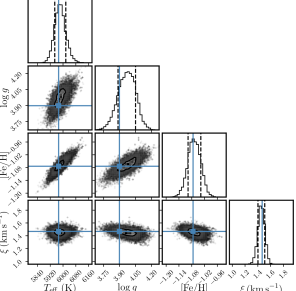
Figure 6: Stellar parameters of the solution satisfying excitation balance at the highest confidence level for G161-73. Lines indicating the values of the parameters are shown overlaid the ensemble solution (posterior distribution) for the star. The $1\sigma$ confidence intervals are shown as the contours in the scatter plots and vertical dashed lines in the histograms.

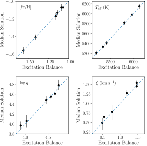
Figure 7: Stellar parameters of the median solution of the ensemble solutions versus stellar parameters of the solution satisfying excitation balance at the highest confidence level for each star. The dotted line is the line of equality, and errorbars represent the $1\sigma$ confidence intervals of the ensemble solutions. The plots demonstrate that the parameters of the solution satisfying excitation balance is within one standard deviation of the median solution for each.

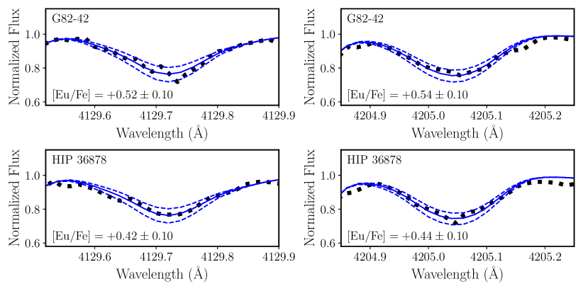
Figure 8: Sample synthesis fits to the Eu II lines at 4129.7 Å (left) and 4205.0 Å (right) for two stars, G82-42 (top) and HIP 36878 (bottom). Observed spectra are shown as dotted lines, best fits to the observed spectra as solid lines, and $\pm 0.10\;\mathrm{dex}$ the best fits as dashed lines.

3.4 Spectral Synthesis: Europium

While we used SPAE to analyze the majority of the elements we discuss in this work, we took a separate approach to deriving the abundances of the predominately $r$-process element Eu. We derived Eu abundances using spectrum synthesis of the Eu II lines at 4129.7 and 4205.0 Å. Other lines typically used for Eu abundances, such as $\lambda 3724$, $\lambda 3819$, $\lambda 6437$, and $\lambda 6645$, were not detected in our spectra. Synthetic spectra were fit to the observed spectra using the synth driver of MOOG, along with a stellar model characterized by the parameters and metallicities from SPAE. Linelists for the 4205 and 4130 Å regions were assembled using Linemake, which includes the atomic data for the Eu II lines from Lawler et al. (2001); we adopted isotopic ratios of 47.8% and 52.2% for ${}^{152}\mathrm{Eu}$ and ${}^{153}\mathrm{Eu}$, respectively, also from Lawler et al. (2001).

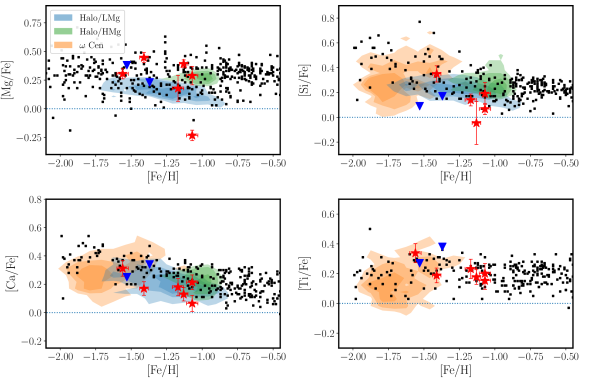
Figure 9: Abundances of $\alpha$-elements as a function of metallicity. G21-22 abundances are given as red stars with error bars representing the final adopted uncertainties listed in Table 4. The blue and green contours represent the abundances of halo stars designated as likely to have been accreted by the Milky Way (LMg) and to have formed in situ (HMg), respectively, from Hayes et al. (2018). The orange contour represents the abundances of the large sample of $\omega$ Cen stars from Johnson & Pilachowski (2010). Blue inverted triangles are abundances of the two stars classified as part of Gaia-Enceladus from Monty et al. (2020). Black squares are general halo star abundances from Venn et al. (2004), Reddy et al. (2006), Nissen & Schuster (2010), Ishigaki et al. (2012), and Roederer et al. (2014).

The linelist was further adjusted by changing slightly the transition probabilities and wavelengths of a handful of lines in the $\lambda 4130$ and $\lambda 4205$ regions to fit a high-quality solar spectrum (Schuler et al., 2015) obtained with the W.M. Keck Observatory and High Resolution Echelle Spectrometer (HIRES; Vogt et al., 1994). None of the atomic parameters of the Eu lines were altered during this process.

Examples of the synthetic fits to the Eu lines are shown in Figure 8. These lines are found in the bluer wavelength regions of our spectra and thus are characterized by lower S/N ratio compared to the redder regions where the rest of the metal lines are measured. The effect of the lower S/N on the Eu lines themselves can be seen in Figure 8. Nonetheless, we measured consistent [Eu/Fe] abundances from each line for each star. The derived [Eu/Fe] abundances are given in Table 6. We adopted a conservative abundance uncertainty of $\pm 0.10\,\mathrm{dex}$ for each star.

Table 6: Europium Abundances

Star		$\mathrm{[Eu/Fe]}_{4129}$		$\mathrm{[Eu/Fe]}_{4205}$		$<\mathrm{[Eu/Fe]}>$
G02-38		+0.53		+0.55		+0.54
G82-42		+0.52		+0.54		+0.53
G108-48		+0.57		+0.60		+0.59
G119-64		+0.50		+0.50		+0.50
G161-73		+0.35		+0.33		+0.34
HIP 36878		+0.42		+0.44		+0.43

4 Discussion

Silva et al. (2012) designated G03-37, G18-39, and G21-22 as moving groups based on stellar density contours in kinematic-metallicity ([Fe/H] vs. $V_{\mathrm{rot}}$) and kinematic (Bottlinger and Toomre) diagrams constructed using Strömgren photometry, radial velocities, and proper motions, mostly obtained from disparate literature sources. We have reproduced this analysis with complete six-dimensional phase space information from Gaia EDR3; the related kinematic and integrals of motion diagrams are shown in Figure 1. Such diagrams are helpful in identifying smaller stellar associations (e.g., Yuan et al., 2020; Limberg et al., 2021), as well as larger structures (e.g., Helmi, 2020), because related stars will generally cluster together in the metallicity and kinematic phase space.

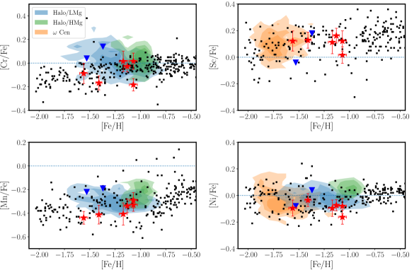
Figure 10: Abundances of Fe-Peak elements as a function of metallicity. Symbols and sources are the same as given in Figure 9. Additional halo star abundances from Ishigaki et al. (2013) are also included.

As an example, in Figure 1 we include 75 stars of the GL-4 halo substructure identified by Li et al. (2019). These stars form a tight group in the integrals of motion and occupy narrow regions in the velocity spaces. If G03-37, G18-39, and G21-22 were true moving groups, a similar degree of clustering would be expected. However, this is not observed for G03-37 nor G18-39, both of which demonstrate larger scatter than GL-4 in the four diagnostics of Figure 1. The G21-22 stars also do not cluster tightly together, although the scatter is reduced compared to the other groups.

With the assumption that moving group stars should not only share common space motions but also compositions, detailed chemical abundance analysis is a powerful tool to complement a dynamical analysis of putative moving group members. Each alone may not be definitive in identifying bona fide members. With the Gaia-based dynamical analysis shown in Figure 1, as well as the orbital analysis shown in Figure 2, seemingly ruling out G03-37 and G18-39 as moving groups but leaving open the possibility for G21-22, we derived detailed abundances for the six stars in that group.

Figure 11: Abundances of the odd-$Z$ elements Na, Al, and V as a function of metallicity. Symbols and sources are the same as given in Figure 9, except for Al, where the orange contour for $\omega$ Cen stars has been replaced with orange circles due to the paucity of these stars with Al abundances. Additional halo star abundances from Ishigaki et al. (2013) are also included.

In Figures 9, 10, 11, and 12, we plot the abundances of $\alpha$- (Mg I, Si I, Ca I, and Ti I), Fe-Peak (Cr I, Sc II, Mn I, and Ni I), odd-$Z$ (Na I, Al I, and V I), and $n$-capture (Ba II and Eu II) elements, respectively, versus [Fe/H] for the six G21-22 stars and other stars in the Galactic halo. Focusing on the G21-22 stars only, it is clear that the six do not compose a chemically homogeneous group. Four stars (G82-42, G108-48, G161-73, and HIP 36878) are characterized by higher metallicities, $\mathrm{[Fe/H]}\approx-1.1$, while the other two are more metal poor at $\mathrm{[Fe/H]}\approx-1.4$ (G02-38) and $\approx-1.6$ (G119-64). For the other elements, their abundances relative to Fe demonstrate mild scatter among the six stars, but nothing unusual is apparent, with the possible exception of the Mg abundance of G108-48. For the metal-rich group, some abundances are consistent within the $1\sigma$ confidence intervals among the stars (Si, Ti, V, Mn, Ni) while some are not (Na, Mg, Ca, Sc, Cr, Ba, Eu).

Taken together, the kinematic metrics and detailed compositions of the G21-22 stars strongly suggest that this collection of stars does not constitute a moving group of stars with a common origin. Given the grouping of four stars in kinematic phase space (Figure 1) and the grouping of four at a metallicity $\mathrm{[Fe/H]}\approx-1.1$, it is possible that a subset of the six stars are members of a moving group. However, the stars in each group are not the same. One of the kinematically similar stars (G02-38) is in the metal-poor group, and the star (G108-48) with the most dissimilar kinematic properties is in the metal-rich group.

4.1 On the Origins of the G21-22 Stars

By comparing the kinematic properties of the G21-22 stars to the models of Meza et al. (2005), Silva et al. (2012) suggest that the stars may be related to the tidal debris of the long hypothesized $\omega$ Cen accretion event (Freeman, 1993) or some other accreted dwarf galaxy. Schuster et al. (2019) offer an alternate explanation, implying the stars formed in situ in the Galaxy and are now trapped in orbital resonances created by the Galactic bar (see also Amarante et al., 2020).

In a search for metal-rich Gaia-Enceladus stars, Zhao & Chen (2021) compare the maximum height above or below the Galactic plane ($z_{\mathrm{max}}$) to the mean Galactic distance ($R_{\mathrm{m}}=R_{\mathrm{apo}}+R_{\mathrm{peri}}/2$, where $R_{\mathrm{apo}}$ is the apocenter distance and $R_{\mathrm{peri}}$ is the pericenter distance) for a sample of stars that includes the star G21-22, after which the putative G21-22 moving group was named. The features of the resulting Zhao & Chen (2021) plot (their figure 7) are similar to those found by Amarante et al. (2020), who compare $z_{\mathrm{max}}$ to $R_{\mathrm{apo}}$ (their figure B1).

Amarante et al. (2020) use newly derived stellar halo and thick-disk fractions, and new stellar kinematics with the Galaxia population synthesis model (Sharma et al., 2011), to conclude that this $z_{\mathrm{max}}$-$R_{\mathrm{apo}}$ relation is a natural consequence of resonant effects. However, Haywood et al. (2018) examine the blue and red sequences of the Gaia HR diagram Gaia Collaboration et al. (2018b) and find a similar relation for $z_{\mathrm{max}}$-$R_{\mathrm{R2D,max}}$ (the apocenter distance projected on the Galactic plane) and, based on this and other dynamical and orbital properties, conclude the blue sequence stars are possible relics of a significant accretion event experienced by the Galaxy.

We attempted to determine the origins of the G21-22 stars by comparing their stellar properties to other stars in the Milky Way halo in kinematic and chemical space. While it is generally accepted that at least part of the halo has been populated by accretion events (e.g., Helmi, 2020), some recent studies suggest that it was built entirely by accretion (Helmi et al., 2017; Naidu et al., 2020). This raises the possibility that the G21-22 stars can be associated to one or more of these structures, each of which occupies a characteristic region in integrals of motion, particularly $E$-$L_{\mathrm{z}}$ (Naidu et al., 2020).

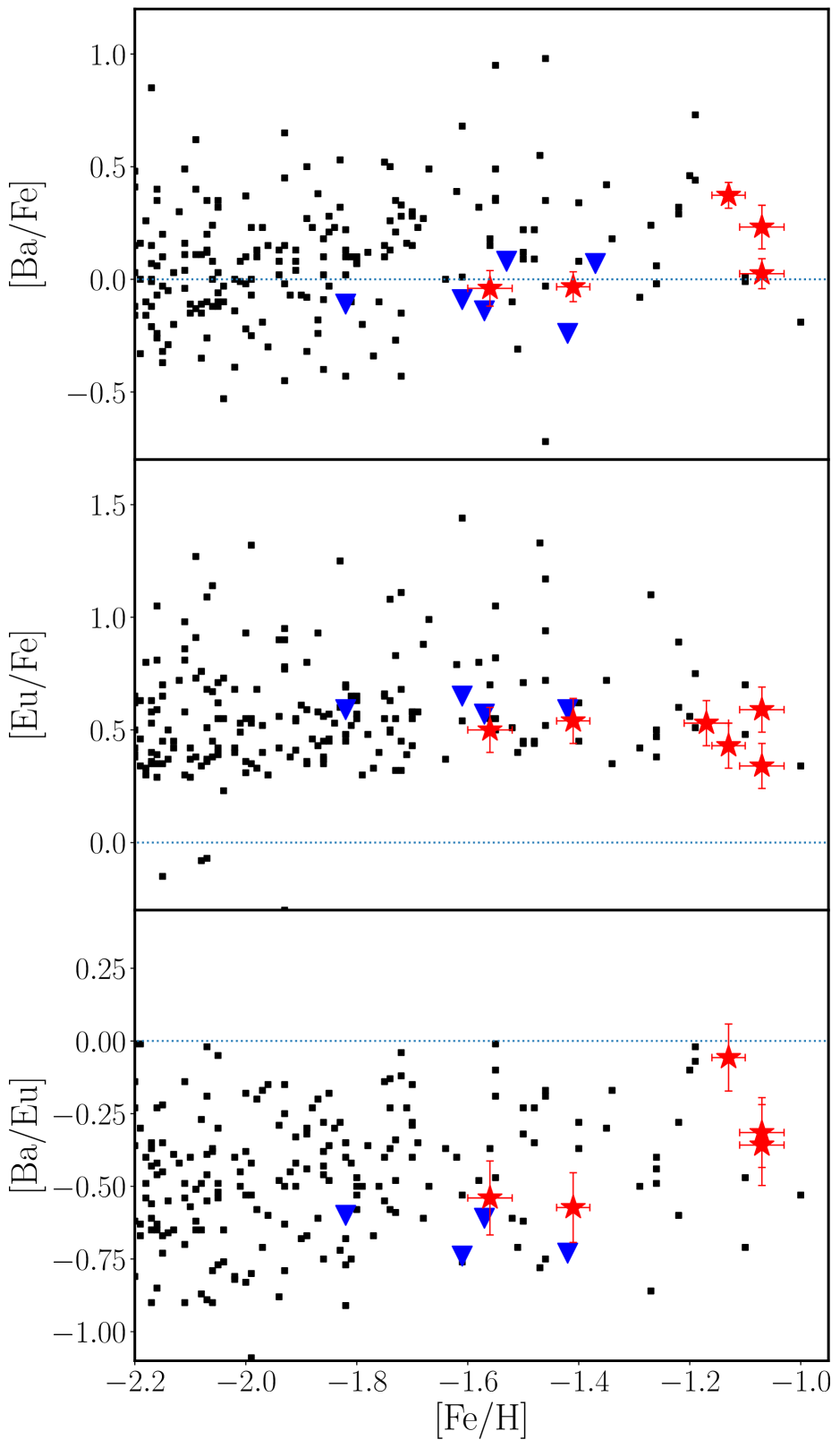
Figure 12: Abundances of Ba, Eu, and Ba relative to Eu as a function of metallicity. Symbols are the same as given in Figure 9 with the following sources: Gaia-Enceladus– Monty et al. (2020) and Aguado et al. (2021); Halo– Gudin et al. (2021); Sagittarius– Hansen et al. (2018).

Naidu et al. (2020) derived their integrals of motion using the same Galactic model as we did (see Section 2). Using these authors’ results as a guide, we can eliminate Sagittarius, Sequoia, Helmi stream, and Thamnos as progenitors of the six G21-22 stars based on their positions in the $E$-$L_{\mathrm{z}}$ and $V_{\phi}$-$V_{\mathrm{r}}$ planes. There is no overlap between these structures and the stars.

The kinematic properties of the stars are consistent with the lower density regions of the high-$\alpha$ disk and in situ halo component of Naidu et al. (2020), but they do not meet the metalicity cutoff set by these authors to distinguish it from the metal-weak thick disk (MWTD), which is taken to be the metal-poor extension of the high-$\alpha$ disk. Conversely, two of the G21-22 stars fall in the [$\alpha$/Fe]-[Fe/H] selection box set for the MWTD, but as we show in Figure 1, the stars are clearly part of the halo and are not consistent with the MWTD in any of the kinematic spaces.

This leaves Gaia-Enceladus, which has been tied to greater than 50% of the Galactic halo (Mackereth et al., 2019), as the possible progenitor. Indeed, the six G21-22 stars are consistent with Gaia-Enceladus in four key diagnostics presented by Naidu et al. (2020): they have eccentricities $e\geq 0.77$ (see Table 8), which is larger than the cutoff value of $e=0.7$, and they overlap with Gaia-Enceladus stars in the $E$-$L_{\mathrm{z}}$, $V_{\phi}$-$V_{\mathrm{r}}$, and [$\alpha$/Fe]-[Fe/H] spaces. Moreover, these stars’ metallicities ([Fe/H]) are within about $1\sigma$ of the mean metallicty of the structure, depending on the value considered (e.g., Vincenzo et al., 2019; Matsuno et al., 2019; Naidu et al., 2020).

To investigate the six G21-22 stars in chemical space, their abundances are plotted with those of general halo populations and $\omega$ Cen in Figures 9, 10, 11, and 12. The general halo population includes stars observed by APOGEE and deemed by Hayes et al. (2018) to have likely been accreted by the Milky Way early in its history (labeled the low-Mg population, LMg) and to have formed in situ, possibly as part of the thick disk (labeled the high-Mg population, HMg). The remaining halo stars are found in Venn et al. (2004), Reddy et al. (2006), Nissen & Schuster (2010), Ishigaki et al. (2012), Ishigaki et al. (2013), and Roederer et al. (2014). Abundances of $\omega$ Cen stars are from Johnson & Pilachowski (2010).

The abundances of $\omega$ Cen, LMg, and HMg occupy distinct regions of the abundance plots, although there is some overlap between LMg and both $\omega$ Cen (at low-[Fe/H]) and HMg (at high-[Fe/H]) for some elements. The G21-22 stars follow the general halo trend, which spans across the $\omega$ Cen, LMg, and HMg stars, and cannot be definitively assigned to any of the three. The abundances of the two more metal-poor stars– G02-38 and G119-64– are consistent with those of $\omega$ Cen, raising the possibility that they are part of the cluster’s tidal debris, as suggested by Silva et al. (2012). However, $L_{\mathrm{z}}$ of these stars are inconsistent with the recently discovered Fimbulthul stream, which has been identified as the tidal stream of $\omega$ Cen (Ibata et al., 2019b, a), arguing against an association with the cluster.

The four more metal-rich stars, G82-42, G108-48, G161-73, and HIP 36878, have abundances generally consistent with those of both the LMg and HMg groups. However, given that the kinematics of all six stars are consistent with Gaia-Enceladus and much of the general halo is composed of stars from Gaia-Enceladus, possibly even the LMg stars, we suggest it as the more likely progenitor of the G21-22 stars. If this is indeed the case, the abundances presented here will add to the nascent list of abundances derived for Gaia-Enceladus stars.

5 Conclusions

We used Gaia astrometry and detailed stellar abundances derived from high-resolution VLT/UVES spectroscopy to investigate the authenticity of three candidate halo moving groups– G03-37, G18-39, and G21-22– identified by Silva et al. (2012). The stars from each group evince significant scatter in integrals of motion (energy, angular momentum) and velocities, contrary to the tight clustering seen for members of moving groups. Moreover, stellar orbits of the stars integrated backward in a Galactic potential over 200 Myr are found to deviate from kinematically coherent orbits, suggesting the stars did not have common space motions in the past. These kinematic diagnostics are counter to what is expected for bona fide moving group stars.

Choosing the putative moving group showing the least scatter in the integrals of motion, we conducted a detailed abundance analysis of the six stars in our G21-22 sample to further investigate the nature of this group. We derived the abundances of 14 elements, including $\alpha$-, Fe-peak, odd-$Z$, and neutron-capture elements, and find that the stars are not chemically homogeneous. Therefore, using the definition of a moving group as a stellar association with a shared formation history, shared space motions, and shared compositions, we concluded that G03-37, G18-39, and G21-22 are not genuine moving groups based on their assigned stars’ discordance in the integrals of motion, integrated orbits, and in the case of G21-22, compositions.

By comparing the integrals of motion of the six stars of G21-22 to those of known and newly discovered structures in the halo presented in Naidu et al. (2020), we tentatively associated the G21-22 stars with the Gaia-Enceladus accretion event. They overlap with Gaia-Enceladus in five key kinematic and chemical diagnostics, while being inconsistent with other major halo structures. If their association is confirmed, the detailed abundances presented here will be valuable in the continued characterization of Gaia-Enceladus and the evolution of the Galactic halo.

While integrals of motion are well established diagnostics for identifying large stellar structures accreted by the Galaxy (e.g., Helmi & de Zeeuw, 2000; Simpson et al., 2019), uncertainties in astrometric parameters can lead to fallacious kinematic quantities that result in uncertain conclusions for smaller associations such as moving groups. Detailed stellar abundances can be used to chemically tag groups of stars, but for stars with disparate positions in the Galaxy– like moving group stars– similar compositions alone may be insufficient to definitely conclude that they share a common formation history. As we have demonstrated, however, the combination of kinematic and chemical information is much more effective at identifying truly conatal populations than either alone.

Appendix A Gaia EDR3 Astrometry and Derived Kinematic Properties of G03-37, G18-39, and G21-22

Table 7 presents the complete six-dimensional phase space information from the early third Gaia data release (EDR3; Gaia Collaboration et al., 2021; Lindegren et al., 2021) for each star identified by Silva et al. (2012) for the three candidate moving groups G03-37, G18-39, and G21-22. The stars were crossed matched in Gaia EDR3 using identifications and positional data from Silva et al. (2012) and Schuster et al. (2006).

Table 7: Observed Gaia EDR3 Characteristics of Halo Moving Group Stars

Star	$\alpha$		$\delta$		$\mu_{\alpha}$		$\mu_{\delta}$	$\varpi$	RV
					(mas yr-1)		(mas yr-1)	(mas)	(km s-1)
G03-37
LP659-016	06:07:22.84	$-$07:10:31.0	$140.85\pm 0.05$	$-120.93\pm 0.05$	$4.18\pm 0.05$	$179.6\pm 2.1$
LP685-044	16:41:57.4	$-$07:52:36.8	$-236.17\pm 0.02$	$-166.37\pm 0.02$	$4.28\pm 0.02$	$\cdots$
G03-37	02:03:02.23	$+$08:51:56.4	$143.31\pm 0.02$	$-98.64\pm 0.02$	$2.45\pm 0.02$	$-83.0\pm 1.6$
G05-36	03:27:00.07	$+$23:46:30.4	$263.00\pm 0.02$	$-344.70\pm 0.01$	$5.76\pm 0.01$	$-9.1\pm 0.3$
G51-07	08:20:06.83	$+$34:42:10.6	$14.54\pm 0.01$	$-377.11\pm 0.01$	$8.36\pm 0.02$	$80.9\pm 3.9$
G53-41	10:27:24.04	$+$01:23:55.4	$-186.34\pm 0.02$	$-294.81\pm 0.02$	$6.06\pm 0.02$	$88.8\pm 0.5$
G142-44	19:38:52.9	$+$16:25:31.1	$-197.36\pm 0.03$	$-185.98\pm 0.03$	$9.05\pm 0.03$	$\cdots$
G170-56	17:38:15.39	$+$18:33:22.2	$-187.82\pm 0.01$	$-203.90\pm 0.01$	$7.68\pm 0.01$	$-239.4\pm 0.5$
G172-61	01:34:23.28	$+$48:44:26.5	$363.98\pm 0.17$	$-57.95\pm 0.16$	$9.44\pm 0.17$	$-203.4\pm 1.9$
G272-122	01:54:32.33	$-$18:27:13.0	$169.11\pm 0.01$	$-147.24\pm 0.01$	$3.61\pm 0.02$	$-15.3\pm 2.0$
HIP 22068	04:44:49.13	$-$32:52:40.0	$352.44\pm 0.01$	$-190.26\pm 0.02$	$7.20\pm 0.01$	$150.2\pm 0.3$
HIP 59490	12:12:01.12	$+$13:15:33.0	$-218.30\pm 0.03$	$-439.48\pm 0.02$	$7.45\pm 0.03$	$99.5\pm 0.3$
HIP 62108	12:43:42.89	$-$44:40:31.8	$-220.73\pm 0.02$	$-17.45\pm 0.01$	$6.80\pm 0.02$	$222.6\pm 0.8$
HIP 69232	14:10:26.70	$-$13:56:11.6	$-339.94\pm 0.04$	$-459.56\pm 0.04$	$7.11\pm 0.04$	$120.2\pm 1.7$
LTT5864	14:46:27.05	$-$35:21:31.5	$-465.91\pm 0.02$	$-246.62\pm 0.02$	$11.19\pm 0.02$	$-139.9\pm 1.2$
G18-39
BD-035166	21:17:18.91	$-$02:44:58.7	$-101.40\pm 0.02$	$-243.28\pm 0.01$	$3.91\pm 0.02$	$-126.9\pm 0.4$
CD-249840	11:36:02.67	$-$24:52:25.0	$-17.91\pm 0.02$	$-211.86\pm 0.02$	$3.63\pm 0.02$	$164.7\pm 0.7$
CD-482445	06:41:26.76	$-$48:13:11.4	$65.05\pm 0.02$	$217.54\pm 0.02$	$5.37\pm 0.01$	$320.8\pm 0.5$
LP490-061	10:43:59.20	$+$12:48:03.8	$-147.43\pm 0.04$	$-97.59\pm 0.03$	$2.38\pm 0.04$	$216.3\pm 3.5$
LP636-003	20:45:01.20	$-$01:40:58.4	$-34.78\pm 0.02$	$-179.62\pm 0.02$	$2.57\pm 0.02$	$\cdots$
LP709-053	02:12:02.41	$-$14:00:29.7	$266.30\pm 0.03$	$-63.26\pm 0.02$	$3.65\pm 0.03$	$-31.4\pm 1.3$
LP877-025	22:53:29.9	$-$23:54:53.6	$-30.32\pm 0.03$	$-396.54\pm 0.03$	$5.53\pm 0.04$	$81.0\pm 1.0$
G10-03	11:10:02.8	$-$02:47:33.0	$144.92\pm 0.02$	$-472.29\pm 0.01$	$9.91\pm 0.02$	$203.1\pm 0.6$
G15-24	15:30:41.34	$+$08:23:38.6	$-391.30\pm 0.02$	$-116.91\pm 0.01$	$6.56\pm 0.02$	$-88.5\pm 0.5$
G18-39	22:18:36.81	$+$08:26:43.3	$283.28\pm 0.02$	$-102.14\pm 0.02$	$6.38\pm 0.02$	$-233.9\pm 0.6$
G31-26	00:08:20.03	$-$05:14:57.0	$352.95\pm 0.03$	$-131.29\pm 0.02$	$5.16\pm 0.03$	$-216.8\pm 1.4$
G34-45	01:42:48.85	$+$22:36:57.0	$74.07\pm 0.02$	$-301.57\pm 0.01$	$7.07\pm 0.02$	$-272.1\pm 6.9$
G36-47	02:57:20.15	$+$26:16:49.7	$259.58\pm 0.02$	$-226.55\pm 0.02$	$4.66\pm 0.03$	$89.5\pm 0.4$
G66-30	14:50:07.49	$+$00:50:25.5	$-291.58\pm 0.15$	$-101.42\pm 0.13$	$6.65\pm 0.14$	$-114.5\pm 5.1$
G70-33	01:03:54.63	$-$03:51:15.3	$339.62\pm 0.02$	$-64.68\pm 0.02$	$4.14\pm 0.02$	$-82.5\pm 3.0$
G86-39	05:23:12.04	$+$33:10:51.3	$391.73\pm 0.02$	$-655.36\pm 0.02$	$12.66\pm 0.02$	$214.7\pm 0.6$
G87-13	06:54:56.36	$+$35:30:54.8	$52.69\pm 0.02$	$-237.88\pm 0.02$	$4.06\pm 0.02$	$206.6\pm 2.5$
G89-14	07:22:31.61	$+$08:49:08.7	$151.20\pm 0.03$	$-269.47\pm 0.02$	$4.40\pm 0.03$	$-38.5\pm 1.7$
G98-53	06:13:49.85	$+$33:24:56.9	$23.21\pm 0.02$	$-325.84\pm 0.01$	$5.46\pm 0.02$	$144.8\pm 1.0$
G120-15	11:06:20.13	$+$31:12:47.5	$-194.82\pm 0.02$	$-129.13\pm 0.02$	$2.98\pm 0.02$	$130.3\pm 0.3$
G157-85	23:36:31.51	$-$08:25:54.9	$260.95\pm 0.06$	$-146.97\pm 0.05$	$3.95\pm 0.06$	$-69.1\pm 2.0$
G176-53	11:46:33.68	$+$50:52:45.9	$-868.72\pm 0.01$	$-544.10\pm 0.01$	$14.16\pm 0.02$	$64.9\pm 0.4$
G187-30	21:11:17.69	$+$33:31:29.8	$502.72\pm 0.01$	$159.62\pm 0.02$	$10.18\pm 0.02$	$-340.2\pm 0.7$
HD 3567	00:38:31.96	$-$08:18:42.1	$20.63\pm 0.03$	$-546.54\pm 0.03$	$8.52\pm 0.02$	$-46.8\pm 0.3$
HD 101063	11:37:40.02	$-$28:51:05.1	$-313.63\pm 0.01$	$-15.67\pm 0.01$	$4.11\pm 0.02$	$183.2\pm 0.4$
G21-22
LP808-022	17:50:36.52	$-$16:59:06.1	$-51.84\pm 0.02$	$-213.58\pm 0.02$	$3.02\pm 0.02$	$\cdots$
G02-38	01:26:55.15	$+$12:00:20.0	$-12.21\pm 0.03$	$-358.99\pm 0.02$	$5.49\pm 0.02$	$-171.9\pm 0.7$
G21-22	18:39:09.54	$+$00:07:07.1	$-163.73\pm 0.02$	$-445.51\pm 0.01$	$6.69\pm 0.02$	$58.9\pm 0.6$
G82-42	04:42:00.01	$-$04:16:52.0	$1.92\pm 0.01$	$-344.68\pm 0.01$	$4.78\pm 0.01$	$-7.8\pm 0.9$
G108-48	07:01:36.89	$+$06:24:17.9	$11.39\pm 0.02$	$-676.01\pm 0.01$	$8.12\pm 0.02$	$-86.9\pm 0.4$
G116-45	09:44:38.16	$+$38:36:34.5	$212.25\pm 0.02$	$-239.66\pm 0.02$	$4.39\pm 0.02$	$-32.9\pm 0.9$
G119-64	11:12:48.09	$+$35:43:35.7	$71.00\pm 0.02$	$-510.84\pm 0.02$	$7.28\pm 0.02$	$-195.0\pm 0.4$
G139-16	17:09:47.21	$+$08:04:19.9	$-160.03\pm 0.01$	$-362.10\pm 0.01$	$5.08\pm 0.01$	$39.7\pm 1.2$
G146-56	10:39:50.60	$+$42:09:01.7	$87.08\pm 0.02$	$-208.15\pm 0.01$	$3.56\pm 0.01$	$\cdots$
G154-25	17:50:36.52	$-$16:59:06.1	$-51.84\pm 0.02$	$-213.58\pm 0.02$	$3.02\pm 0.02$	$\cdots$
G161-73	09:45:37.99	$-$04:40:32.5	$152.15\pm 0.02$	$-250.73\pm 0.02$	$4.37\pm 0.02$	$120.4\pm 0.7$
HIP 36878	07:34:53.41	$-$10:23:17.7	$424.66\pm 0.01$	$-481.99\pm 0.01$	$9.04\pm 0.02$	$80.3\pm 0.8$

Table 8 presents veloicities and integrals of motion for each star identified by Silva et al. (2012) for the three candidate moving groups G03-37, G18-39, and G21-22. The quantities have been derived using the Galactic modeling framework of Astropy v4.0 (Astropy Collaboration et al., 2013, 2018) and the Galactic modeling code, gala (Price-Whelan, 2017), with its built-in Galactic potential MilkyWayPotential (see Table 8). This model combines the disk model from Bovy (2015) with a spherical NFW profile (Navarro et al., 1997).

Table 8: Derived Characteristics of Halo Moving Group Stars

Star	$V_{\rho}$		$V_{z}$		$V_{\phi}$		$U$		$V$	$W$	E	$L_{z}$	$e$
	(km s-1)		(km s-1)		(km s-1)		(km s-1)		(km s-1)	(km s-1)	($10^{5}$ km2 s-2)	($10^{3}$ kpc km s-1)
G03-37
LP659-016	37.8	47.7	22.8	-40.4	-263.7	47.0	-1.53	0.189	0.90
LP685-044	$\cdots$	$\cdots$	$\cdots$	$\cdots$	$\cdots$	$\cdots$	$\cdots$	$\cdots$	$\cdots$
G03-37	62.8	36.5	92.7	-67.1	-332.1	35.7	-1.48	0.774	0.62
G05-36	43.4	-64.6	99.6	-46.7	-339.7	-65.4	-1.47	0.824	0.57
G51-07	48.4	18.8	-25.6	-51.4	-214.8	18.0	-1.54	-0.211	0.90
G53-41	25.0	-104.7	15.6	-27.4	-256.2	-105.4	-1.50	0.127	0.79
G142-44	$\cdots$	$\cdots$	$\cdots$	$\cdots$	$\cdots$	$\cdots$	$\cdots$	$\cdots$	$\cdots$
G170-56	59.0	-35.4	37.0	-62.1	-276.8	-36.2	-1.54	0.297	0.84
G172-61	0.8	57.8	24.4	-4.1	-264.8	57.2	-1.54	0.200	0.88
G272-122	29.8	45.1	44.0	-32.7	-284.4	44.3	-1.53	0.361	0.81
HIP 22068	-0.5	71.2	50.9	-2.0	-291.2	70.6	-1.52	0.416	0.76
HIP 59490	-28.6	14.0	81.8	26.1	-322.0	13.5	-1.52	0.665	0.66
HIP 62108	4.8	61.1	19.3	-7.5	-259.7	60.4	-1.55	0.155	0.90
HIP 69232	-31.8	-37.0	151.3	30.0	-391.4	-37.6	-1.44	1.215	0.37
LTT5864	214.6	-45.3	-126.1	-218.1	-115.5	-46.5	-1.25	-1.015	0.71
G18-39
BD-035166	-165.5	38.3	58.6	161.3	-302.2	38.1	-1.41	0.468	0.82
CD-249840	-145.3	-117.5	24.5	143.3	-260.9	-117.8	-1.39	0.198	0.81
CD-482445	225.4	-5.1	44.1	-227.3	-289.1	-6.3	-1.30	0.360	0.90
LP490-061	227.7	-2.5	87.4	-228.6	-332.7	-3.7	-1.25	0.722	0.81
LP636-003	$\cdots$	$\cdots$	$\cdots$	$\cdots$	$\cdots$	$\cdots$	$\cdots$	$\cdots$	$\cdots$
LP709-053	168.5	123.4	38.8	-171.7	-279.3	122.4	-1.33	0.320	0.75
LP877-025	-188.7	-88.6	41.0	185.9	-282.4	-88.7	-1.34	0.330	0.84
G10-03	-160.8	80.8	19.8	157.9	-259.0	80.6	-1.40	0.161	0.91
G15-24	132.4	73.8	18.3	-135.5	-258.2	72.8	-1.45	0.147	0.87
G18-39	176.4	-3.5	19.0	-179.6	-256.8	-4.6	-1.41	0.154	0.95
G31-26	200.4	107.0	89.8	-204.4	-328.2	105.8	-1.26	0.730	0.72
G34-45	-190.7	34.8	44.6	187.3	-286.6	34.7	-1.36	0.366	0.88
G36-47	179.5	-83.6	48.6	-182.6	-287.2	-84.7	-1.34	0.403	0.82
G66-30	149.0	-21.7	-60.1	-151.9	-180.4	-22.7	-1.44	-0.483	0.80
G70-33	248.2	73.7	57.4	-251.8	-295.6	72.4	-1.21	0.470	0.86
G86-39	230.7	-15.6	15.3	-233.5	-255.4	-16.9	-1.29	0.126	0.97
G87-13	195.0	19.2	37.5	-197.9	-277.9	18.1	-1.35	0.313	0.90
G89-14	-207.5	18.2	29.2	204.9	-266.9	18.1	-1.33	0.243	0.93
G98-53	149.8	-85.6	11.7	-152.4	-252.0	-86.7	-1.40	0.097	0.89
G120-15	234.9	10.8	60.0	-237.5	-301.5	9.6	-1.26	0.495	0.87
G157-85	184.1	-76.6	52.7	-187.4	-290.6	-77.8	-1.35	0.427	0.81
G176-53	209.5	62.3	18.5	-212.6	-258.4	61.2	-1.32	0.151	0.91
G187-30	263.0	-54.1	66.9	-266.5	-304.1	-55.5	-1.18	0.542	0.87
HD 3567	-163.5	-47.1	16.7	160.6	-257.8	-47.4	-1.42	0.136	0.93
HD 101063	259.3	-12.9	49.9	-260.9	-296.7	-14.2	-1.22	0.403	0.91
G21-22
LP808-022	$\cdots$	$\cdots$	$\cdots$	$\cdots$	$\cdots$	$\cdots$	$\cdots$	$\cdots$	$\cdots$
G02-38	-224.2	-57.7	29.6	221.2	-272.2	-57.8	-1.29	0.243	0.90
G21-22	-239.7	-30.7	4.2	236.8	-246.9	-30.7	-1.28	0.034	0.99
G82-42	-204.6	-130.6	2.8	202.1	-241.6	-130.7	-1.26	0.023	0.87
G108-48	-243.6	-171.8	35.0	241.4	-273.6	-171.8	-1.11	0.288	0.77
G116-45	-234.6	137.1	-11.0	231.3	-229.0	137.0	-1.18	-0.091	0.85
G119-64	-233.9	-121.6	46.6	231.4	-286.8	-121.7	-1.20	0.381	0.83
G139-16	-227.4	10.4	56.0	223.8	-298.7	10.3	-1.30	0.446	0.87
G146-56	$\cdots$	$\cdots$	$\cdots$	$\cdots$	$\cdots$	$\cdots$	$\cdots$	$\cdots$	$\cdots$
G154-25	$\cdots$	$\cdots$	$\cdots$	$\cdots$	$\cdots$	$\cdots$	$\cdots$	$\cdots$	$\cdots$
G161-73	-230.8	45.6	17.1	228.1	-252.8	45.5	-1.28	0.140	0.95
HIP 36878	-203.5	87.6	34.0	200.7	-272.4	87.4	-1.31	0.279	0.87

References

- Aguado et al. (2021) Aguado, D. S., Belokurov, V., Myeong, G. C., et al. 2021, ApJ, 908, L8, doi: 10.3847/2041-8213/abdbb8
- Amarante et al. (2020) Amarante, J. A. S., Smith, M. C., & Boeche, C. 2020, MNRAS, 492, 3816, doi: 10.1093/mnras/staa077
- Asplund et al. (2021) Asplund, M., Amarsi, A. M., & Grevesse, N. 2021, arXiv e-prints, arXiv:2105.01661. https://arxiv.org/abs/2105.01661
- Asplund et al. (2009) Asplund, M., Grevesse, N., Sauval, A. J., & Scott, P. 2009, ARA&A, 47, 481, doi: 10.1146/annurev.astro.46.060407.145222
- Astropy Collaboration et al. (2013) Astropy Collaboration, Robitaille, T. P., Tollerud, E. J., et al. 2013, A&A, 558, A33, doi: 10.1051/0004-6361/201322068
- Astropy Collaboration et al. (2018) Astropy Collaboration, Price-Whelan, A. M., Sipőcz, B. M., et al. 2018, AJ, 156, 123, doi: 10.3847/1538-3881/aabc4f
- Bellm et al. (2019) Bellm, E. C., Kulkarni, S. R., Graham, M. J., et al. 2019, PASP, 131, 018002, doi: 10.1088/1538-3873/aaecbe
- Belokurov et al. (2018) Belokurov, V., Erkal, D., Evans, N. W., Koposov, S. E., & Deason, A. J. 2018, MNRAS, 478, 611, doi: 10.1093/mnras/sty982
- Bensby et al. (2003) Bensby, T., Feltzing, S., & Lundström, I. 2003, A&A, 410, 527, doi: 10.1051/0004-6361:20031213
- Bovy (2015) Bovy, J. 2015, ApJS, 216, 29, doi: 10.1088/0067-0049/216/2/29
- Carollo et al. (2007) Carollo, D., Beers, T. C., Lee, Y. S., et al. 2007, Nature, 450, 1020, doi: 10.1038/nature06460
- Cropper et al. (2018) Cropper, M., Katz, D., Sartoretti, P., et al. 2018, A&A, 616, A5, doi: 10.1051/0004-6361/201832763
- Dark Energy Survey Collaboration et al. (2016) Dark Energy Survey Collaboration, Abbott, T., Abdalla, F. B., et al. 2016, MNRAS, 460, 1270, doi: 10.1093/mnras/stw641
- Dekker et al. (2000) Dekker, H., D’Odorico, S., Kaufer, A., Delabre, B., & Kotzlowski, H. 2000, in Society of Photo-Optical Instrumentation Engineers (SPIE) Conference Series, Vol. 4008, Optical and IR Telescope Instrumentation and Detectors, ed. M. Iye & A. F. Moorwood, 534–545, doi: 10.1117/12.395512
- Eggen (1958) Eggen, O. J. 1958, MNRAS, 118, 65, doi: 10.1093/mnras/118.1.65
- Foreman-Mackey (2016) Foreman-Mackey, D. 2016, The Journal of Open Source Software, 1, 24, doi: 10.21105/joss.00024
- Foreman-Mackey et al. (2013) Foreman-Mackey, D., Hogg, D. W., Lang, D., & Goodman, J. 2013, PASP, 125, 306, doi: 10.1086/670067
- Freeman (1993) Freeman, K. C. 1993, in Astronomical Society of the Pacific Conference Series, Vol. 48, The Globular Cluster-Galaxy Connection, ed. G. H. Smith & J. P. Brodie, 608
- Freudling et al. (2013) Freudling, W., Romaniello, M., Bramich, D. M., et al. 2013, A&A, 559, A96, doi: 10.1051/0004-6361/201322494
- Gaia Collaboration et al. (2018a) Gaia Collaboration, Brown, A. G. A., Vallenari, A., et al. 2018a, A&A, 616, A1, doi: 10.1051/0004-6361/201833051
- Gaia Collaboration et al. (2018b) Gaia Collaboration, Babusiaux, C., van Leeuwen, F., et al. 2018b, A&A, 616, A10, doi: 10.1051/0004-6361/201832843
- Gaia Collaboration et al. (2021) Gaia Collaboration, Brown, A. G. A., Vallenari, A., et al. 2021, A&A, 649, A1, doi: 10.1051/0004-6361/202039657
- Giclas et al. (1975) Giclas, H. L., Burnham, R., J., & Thomas, N. G. 1975, Lowell Observatory Bulletin, 8, 9
- Giclas et al. (1961) Giclas, H. L., Burnham, R., & Thomas, N. G. 1961, Lowell Observatory Bulletin, 6, 61
- Giclas et al. (1959) Giclas, H. L., Slaughter, C. D., & Burnham, R. 1959, Lowell Observatory Bulletin, 4, 136
- Goodman & Weare (2010) Goodman, J., & Weare, J. 2010, Communications in Applied Mathematics and Computational Science, 5, 65, doi: 10.2140/camcos.2010.5.65
- Gudin et al. (2021) Gudin, D., Shank, D., Beers, T. C., et al. 2021, ApJ, 908, 79, doi: 10.3847/1538-4357/abd7ed
- Hansen et al. (2018) Hansen, C. J., El-Souri, M., Monaco, L., et al. 2018, ApJ, 855, 83, doi: 10.3847/1538-4357/aa978f
- Harris et al. (2020) Harris, C. R., Millman, K. J., van der Walt, S. J., et al. 2020, Nature, 585, 357, doi: 10.1038/s41586-020-2649-2
- Hawkins et al. (2015) Hawkins, K., Jofré, P., Masseron, T., & Gilmore, G. 2015, MNRAS, 453, 758, doi: 10.1093/mnras/stv1586
- Hayes et al. (2018) Hayes, C. R., Majewski, S. R., Shetrone, M., et al. 2018, ApJ, 852, 49, doi: 10.3847/1538-4357/aa9cec
- Haywood et al. (2018) Haywood, M., Di Matteo, P., Lehnert, M. D., et al. 2018, ApJ, 863, 113, doi: 10.3847/1538-4357/aad235
- Helmi (2020) Helmi, A. 2020, ARA&A, 58, 205, doi: 10.1146/annurev-astro-032620-021917
- Helmi et al. (2018) Helmi, A., Babusiaux, C., Koppelman, H. H., et al. 2018, Nature, 563, 85, doi: 10.1038/s41586-018-0625-x
- Helmi & de Zeeuw (2000) Helmi, A., & de Zeeuw, P. T. 2000, MNRAS, 319, 657, doi: 10.1046/j.1365-8711.2000.03895.x
- Helmi et al. (2017) Helmi, A., Veljanoski, J., Breddels, M. A., Tian, H., & Sales, L. V. 2017, A&A, 598, A58, doi: 10.1051/0004-6361/201629990
- Hunter (2007) Hunter, J. D. 2007, Computing in Science Engineering, 9, 90, doi: 10.1109/MCSE.2007.55
- Ibata et al. (2019a) Ibata, R. A., Bellazzini, M., Malhan, K., Martin, N., & Bianchini, P. 2019a, Nature Astronomy, 3, 667, doi: 10.1038/s41550-019-0751-x
- Ibata et al. (1994) Ibata, R. A., Gilmore, G., & Irwin, M. J. 1994, Nature, 370, 194, doi: 10.1038/370194a0
- Ibata et al. (2019b) Ibata, R. A., Malhan, K., & Martin, N. F. 2019b, ApJ, 872, 152, doi: 10.3847/1538-4357/ab0080
- Ishigaki et al. (2013) Ishigaki, M. N., Aoki, W., & Chiba, M. 2013, ApJ, 771, 67, doi: 10.1088/0004-637X/771/1/67
- Ishigaki et al. (2012) Ishigaki, M. N., Chiba, M., & Aoki, W. 2012, ApJ, 753, 64, doi: 10.1088/0004-637X/753/1/64
- Johnson & Pilachowski (2010) Johnson, C. I., & Pilachowski, C. A. 2010, ApJ, 722, 1373, doi: 10.1088/0004-637X/722/2/1373
- Johnson & Soderblom (1987) Johnson, D. R. H., & Soderblom, D. R. 1987, AJ, 93, 864, doi: 10.1086/114370
- Kurucz (2011) Kurucz, R. L. 2011, Canadian Journal of Physics, 89, 417, doi: 10.1139/p10-104
- Lawler et al. (2019) Lawler, J. E., Hala, Sneden, C., et al. 2019, ApJS, 241, 21, doi: 10.3847/1538-4365/ab08ef
- Lawler et al. (2001) Lawler, J. E., Wickliffe, M. E., den Hartog, E. A., & Sneden, C. 2001, ApJ, 563, 1075, doi: 10.1086/323407
- Li et al. (2019) Li, H., Du, C., Liu, S., Donlon, T., & Newberg, H. J. 2019, ApJ, 874, 74, doi: 10.3847/1538-4357/ab06f4
- Limberg et al. (2021) Limberg, G., Rossi, S., Beers, T. C., et al. 2021, ApJ, 907, 10, doi: 10.3847/1538-4357/abcb87
- Lindegren et al. (2021) Lindegren, L., Klioner, S. A., Hernández, J., et al. 2021, A&A, 649, A2, doi: 10.1051/0004-6361/202039709
- Lynden-Bell & Lynden-Bell (1995) Lynden-Bell, D., & Lynden-Bell, R. M. 1995, MNRAS, 275, 429, doi: 10.1093/mnras/275.2.429
- Mackereth et al. (2019) Mackereth, J. T., Schiavon, R. P., Pfeffer, J., et al. 2019, MNRAS, 482, 3426, doi: 10.1093/mnras/sty2955
- Majewski et al. (2003) Majewski, S. R., Skrutskie, M. F., Weinberg, M. D., & Ostheimer, J. C. 2003, ApJ, 599, 1082, doi: 10.1086/379504
- Matsuno et al. (2019) Matsuno, T., Aoki, W., & Suda, T. 2019, ApJ, 874, L35, doi: 10.3847/2041-8213/ab0ec0
- Meza et al. (2005) Meza, A., Navarro, J. F., Abadi, M. G., & Steinmetz, M. 2005, MNRAS, 359, 93, doi: 10.1111/j.1365-2966.2005.08869.x
- Monty et al. (2020) Monty, S., Venn, K. A., Lane, J. M. M., Lokhorst, D., & Yong, D. 2020, MNRAS, 497, 1236, doi: 10.1093/mnras/staa1995
- Naidu et al. (2020) Naidu, R. P., Conroy, C., Bonaca, A., et al. 2020, ApJ, 901, 48, doi: 10.3847/1538-4357/abaef4
- Navarrete et al. (2015) Navarrete, C., Chanamé, J., Ramírez, I., et al. 2015, ApJ, 808, 103, doi: 10.1088/0004-637X/808/1/103
- Navarro et al. (1997) Navarro, J. F., Frenk, C. S., & White, S. D. M. 1997, ApJ, 490, 493, doi: 10.1086/304888
- Newberg et al. (2002) Newberg, H. J., Yanny, B., Rockosi, C., et al. 2002, ApJ, 569, 245, doi: 10.1086/338983
- Nissen & Schuster (2010) Nissen, P. E., & Schuster, W. J. 2010, A&A, 511, L10, doi: 10.1051/0004-6361/200913877
- Nissen & Schuster (2011) —. 2011, A&A, 530, A15, doi: 10.1051/0004-6361/201116619
- Placco et al. (2021) Placco, V. M., Sneden, C., Roederer, I. U., et al. 2021, Research Notes of the American Astronomical Society, 5, 92, doi: 10.3847/2515-5172/abf651
- Price-Whelan et al. (2020) Price-Whelan, A., Sipőcz, B., Lenz, D., et al. 2020, adrn/gala: v1.3, v1.3, Zenodo, doi: 10.5281/zenodo.4159870
- Price-Whelan (2017) Price-Whelan, A. M. 2017, The Journal of Open Source Software, 2, 388, doi: 10.21105/joss.00388
- Ramírez et al. (2012) Ramírez, I., Meléndez, J., & Chanamé, J. 2012, ApJ, 757, 164, doi: 10.1088/0004-637X/757/2/164
- Reddy et al. (2006) Reddy, B. E., Lambert, D. L., & Allende Prieto, C. 2006, MNRAS, 367, 1329, doi: 10.1111/j.1365-2966.2006.10148.x
- Ricker et al. (2015) Ricker, G. R., Winn, J. N., Vanderspek, R., et al. 2015, Journal of Astronomical Telescopes, Instruments, and Systems, 1, 014003, doi: 10.1117/1.JATIS.1.1.014003
- Roederer et al. (2014) Roederer, I. U., Preston, G. W., Thompson, I. B., et al. 2014, AJ, 147, 136, doi: 10.1088/0004-6256/147/6/136
- Sakari et al. (2019) Sakari, C. M., Roederer, I. U., Placco, V. M., et al. 2019, ApJ, 874, 148, doi: 10.3847/1538-4357/ab0c02
- Schuler & Andrews (2021) Schuler, S., & Andrews, J. 2021, SPAE: Stellar Parameters, Abundances, and Errors. https://github.com/simon-schuler/SPAE
- Schuler et al. (2011) Schuler, S. C., Flateau, D., Cunha, K., et al. 2011, ApJ, 732, 55, doi: 10.1088/0004-637X/732/1/55
- Schuler et al. (2015) Schuler, S. C., Vaz, Z. A., Katime Santrich, O. J., et al. 2015, ApJ, 815, 5, doi: 10.1088/0004-637X/815/1/5
- Schuster et al. (2006) Schuster, W. J., Moitinho, A., Márquez, A., Parrao, L., & Covarrubias, E. 2006, A&A, 445, 939, doi: 10.1051/0004-6361:20053796
- Schuster et al. (2019) Schuster, W. J., Moreno, E., & Fernández-Trincado, J. G. 2019, in Dwarf Galaxies: From the Deep Universe to the Present, ed. K. B. W. McQuinn & S. Stierwalt, Vol. 344, 134–138, doi: 10.1017/S174392131800683X
- Schuster et al. (2012) Schuster, W. J., Moreno, E., Nissen, P. E., & Pichardo, B. 2012, A&A, 538, A21, doi: 10.1051/0004-6361/201118035
- Sharma et al. (2011) Sharma, S., Bland-Hawthorn, J., Johnston, K. V., & Binney, J. 2011, ApJ, 730, 3, doi: 10.1088/0004-637X/730/1/3
- Silva et al. (2012) Silva, J. S., Schuster, W. J., & Contreras, M. E. 2012, Rev. Mexicana Astron. Astrofis., 48, 109
- Simpson et al. (2019) Simpson, C. M., Gargiulo, I., Gómez, F. A., et al. 2019, MNRAS, 490, L32, doi: 10.1093/mnrasl/slz142
- Sneden (1973) Sneden, C. 1973, ApJ, 184, 839, doi: 10.1086/152374
- Venn et al. (2004) Venn, K. A., Irwin, M., Shetrone, M. D., et al. 2004, AJ, 128, 1177, doi: 10.1086/422734
- Villanova & Geisler (2011) Villanova, S., & Geisler, D. 2011, A&A, 535, A31, doi: 10.1051/0004-6361/201117552
- Vincenzo et al. (2019) Vincenzo, F., Spitoni, E., Calura, F., et al. 2019, MNRAS, 487, L47, doi: 10.1093/mnrasl/slz070
- Virtanen et al. (2020) Virtanen, P., Gommers, R., Oliphant, T. E., et al. 2020, Nature Methods, 17, 261, doi: 10.1038/s41592-019-0686-2
- Vogt et al. (1994) Vogt, S. S., Allen, S. L., Bigelow, B. C., et al. 1994, in Society of Photo-Optical Instrumentation Engineers (SPIE) Conference Series, Vol. 2198, Instrumentation in Astronomy VIII, ed. D. L. Crawford & E. R. Craine, 362, doi: 10.1117/12.176725
- Willman et al. (2005) Willman, B., Dalcanton, J. J., Martinez-Delgado, D., et al. 2005, ApJ, 626, L85, doi: 10.1086/431760
- Wylie-de Boer et al. (2010) Wylie-de Boer, E., Freeman, K., & Williams, M. 2010, AJ, 139, 636, doi: 10.1088/0004-6256/139/2/636
- Yousefi & Bernath (2018) Yousefi, M., & Bernath, P. F. 2018, ApJS, 237, 8, doi: 10.3847/1538-4365/aacc6a
- Yuan et al. (2020) Yuan, Z., Myeong, G. C., Beers, T. C., et al. 2020, ApJ, 891, 39, doi: 10.3847/1538-4357/ab6ef7
- Zhao & Chen (2021) Zhao, G., & Chen, Y. 2021, Science China Physics, Mechanics, and Astronomy, 64, 239562, doi: 10.1007/s11433-020-1645-5