Sparse Flows: Pruning Continuous-depth Models

Abstract

Continuous deep learning architectures enable learning of flexible probabilistic models for predictive modeling as neural ordinary differential equations (ODEs), and for generative modeling as continuous normalizing flows. In this work, we design a framework to decipher the internal dynamics of these continuous depth models by pruning their network architectures. Our empirical results suggest that pruning improves generalization for neural ODEs in generative modeling. We empirically show that the improvement is because pruning helps avoid mode-collapse and flatten the loss surface. Moreover, pruning finds efficient neural ODE representations with up to 98% less parameters compared to the original network, without loss of accuracy. We hope our results will invigorate further research into the performance-size trade-offs of modern continuous-depth models.

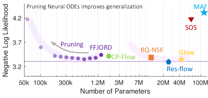
Figure 1: Pruning Neural ODEs improves their generalization with at least 1 order of magnitude less parameters. CIFAR-10 density estimation. Values and methods are described in Table 3.

1 Introduction

The continuous analog of normalizing flows (CNFs) (Chen et al., 2018) efficiently (Grathwohl et al., 2019) maps a latent space to data by ordinary differential equations (ODEs), relaxing the strong constraints over discrete normalizing flows (Rezende and Mohamed, 2015, Dinh et al., 2016, Papamakarios et al., 2017, Kingma and Dhariwal, 2018, Durkan et al., 2019, Huang et al., 2020). CNFs enable learning flexible models by unconstrained neural networks. While recent works investigated ways to improve CNFs’ efficiency (Grathwohl et al., 2019, Finlay et al., 2020, Li et al., 2020), regularize the flows (Yang and Karniadakis, 2020, Onken et al., 2020), or solving their shortcomings such as crossing trajectories (Dupont et al., 2019, Massaroli et al., 2020), less is understood about their inner dynamics during and post training.

In this paper, we set out to use standard pruning algorithms to investigate generalization properties of sparse neural ODEs and continuous normalizing flows. In particular, we investigate how the inner dynamics and the modeling performance of a continuous flow varies if we methodologically prune its neural network architecture. Reducing unnecessary weights of a neural network (pruning) (LeCun et al., 1990, Hassibi and Stork, 1993, Han et al., 2015b, Li et al., 2016) without loss of accuracy results in smaller network size (Hinton et al., 2015, Liebenwein et al., 2021a, b), computational efficiency (Yang et al., 2017, Molchanov et al., 2019, Luo et al., 2017), faster inference (Frankle and Carbin, 2019), and enhanced interpretability (Liebenwein et al., 2020, Lechner et al., 2020a, Baykal et al., 2019a, b). Here, our main objective is to better understand CNFs’ dynamics in density estimation tasks as we increase network sparsity and to show that pruning can improve generalization in neural ODEs.

Figure 2: Pruning enhances generalization of continuous-depth models. Structured pruning (green), unstructured pruning (blue). More details in Section 4.

Pruning improves generalization in neural ODEs.

Our results consistently suggest that a certain ratio of pruning of fully connected neural ODEs leads to lower empirical risk in density estimation tasks, thus obtaining better generalization. We validate this observation on a large series of experiments with increasing dimensionality. See an example here in Figure 2.

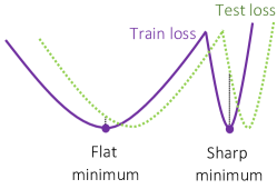
Figure 3: Flat minima result in better generalization compared to sharp minima. Pruning neural ODEs flattens the loss around local minima. Figure is reproduced from Keskar et al. (2017).

Pruning flattens the loss surface of neural ODEs. Additionally, we conduct a Hessian-based empirical investigation on the objective function of the flows-under-test in density estimation tasks to better understand why pruning results in better generalization. We find that for Neural ODEs, pruning decreases the value of the Hessian’s eigenvalues, and as a result, flattens the loss which leads to better generalization, c.f., Keskar et al. (2017) (Figure 3).

Pruning helps avoiding mode-collapse in generative modeling. In a series of multi-modal density estimation tasks, we observe that densely connected CNFs often get stuck in a sharp local minimum (See Figure 3) and as a result, cannot properly distinguish different modes of data. This phenomena is known as mode-collapse. Once we sparsify the flows, the quality of the density estimation task increases significantly and consequently mode-collapse does not occur.

Pruning finds minimal and efficient neural ODE representations. Our framework finds highly optimized and efficient neural ODE architectures via pruning. In many instances, we can reduce the parameter count by 70-98% (6x-50x compression rate). Notably, one cannot directly train such sparse and efficient continuous-depth models from scratch.

2 Background

In this section, we describe the necessary background to construct our framework. We show how to perform generative modeling by continuous depth models using the change of variables formula.

Generative modeling via change of variables.

The change of variables formula uses an invertible mapping $f:\mathbb{R}^{D}\rightarrow\mathbb{R}^{D}$, to wrap a normalized base distribution $p_{z}(\textbf{z})$, to specify a more complex distribution. In particular, given $z\sim p_{z}(\textbf{z})$, a random variable, the log density for function $f(\textbf{z})=\textbf{x}$ can be computed by Dinh et al. (2015):

$$\log p_{x}(\textbf{x})=\log p_{z}(\textbf{z})-\log\det\left|\frac{\partial f(\textbf{z})}{\partial\textbf{z}}\right|,$$ (1)

where $\frac{\partial f(\textbf{z})}{\partial\textbf{z}}$ is the Jacobian of $f$. While theoretically Eq. 1 demonstrates a simple way to finding the log density, from a practical standpoint computation of the Jacobian determinant has a time complexity of $\mathcal{O}(D^{3})$. Restricting network architectures can make its computation more tractable. Examples include designing normalizing flows (Rezende and Mohamed, 2015, Papamakarios et al., 2017, Berg et al., 2018), autoregressive transformations (Kingma et al., 2016, Oliva et al., 2018a, Müller et al., 2019, Wehenkel and Louppe, 2019, Durkan et al., 2019, Jaini et al., 2019), partitioned transformations (Dinh et al., 2016, Kingma and Dhariwal, 2018), universal flows (Kong and Chaudhuri, 2020, Teshima et al., 2020), and the use of optimal transport theorem (Huang et al., 2020).

Alternative to these discrete transformation algorithms, one can construct a generative model similar to (1), and declare $f$ by a continuous-time dynamics (Chen et al., 2018, Grathwohl et al., 2019, Lechner et al., 2020b). Given a sample from the base distribution, one can parametrize an ordinary differential equations (ODEs) by a function $f(\textbf{z}(t),t,\theta)$, and solve the ODE to obtain the observable data. When $f$ is a neural network, the system is called a neural ODE (Chen et al., 2018).

Neural ODEs.

More formally, a neural ODE is defined by finding the solution to the initial value problem (IVP): $\frac{\partial\textbf{z}(t)}{\partial t}=f(\textbf{z}(t),t,\theta)$, $\textbf{z}(t_{0})=\textbf{z}_{0}$, with $\textbf{z}_{0}\sim p_{z_{0}}(\textbf{z}_{0})$, to get $\textbf{z}(t_{n})$ the desired output observations at a terminal integration step $n$ (Chen et al., 2018).

Continuous Normalizing Flows.

If $\textbf{z}(t_{n})$ is set to our observable data, given samples from the base distribution $\textbf{z}_{0}\sim p_{z_{0}}(\textbf{z}_{0})$, the neural ODE described above forms a continuous normalizing flow (CNF). CNFs modify the change in log density by the left hand-side differential equation and as a result the total change in log-density by the right hand-side equation (Chen et al., 2018, Grathwohl et al., 2019):

$$\frac{\partial\log p(\textbf{z}(t))}{\partial t}=-\text{Tr}\left(\frac{\partial f}{\partial\textbf{z}(t)}\right),~{}~{}~{}\log p(\textbf{z}(t_{n}))=\log p(\textbf{z}(t_{0}))-\int_{t_{0}}^{t_{1}}\text{Tr}\left(\frac{\partial f}{\partial\textbf{z}(t)}\right)dt.$$ (2)

The system of two differential equations (the neural ODE ($\frac{\partial\textbf{z}(t)}{\partial t}=f(\textbf{z}(t),t,\theta)$) and (2) can then be solved by automatic differentiation algorithms such as backpropagation through time (Rumelhart et al., 1986, Hasani et al., 2021) or the adjoint sensitivity method (Pontryagin, 2018, Chen et al., 2018). Computation of $\text{Tr}\left(\frac{\partial f}{\partial\textbf{z}(t)}\right)$ costs $\mathcal{O}(D^{2})$. A method called the Free-form Jacobian of Reversible Dynamics (FFJORD) (Grathwohl et al., 2019) improved the cost to $\mathcal{O}(D)$ by using the Hutchinson’s trace estimator (Hutchinson, 1989, Adams et al., 2018). Thus, the trace of the Jacobian can be estimated by: $\text{Tr}\left(\frac{\partial f}{\partial\textbf{z}(t)}\right)=\mathbb{E}_{p(\boldsymbol{\varepsilon})}\left[\boldsymbol{\varepsilon}^{T}\frac{\partial f}{\partial\textbf{z}(t)}\boldsymbol{\varepsilon}\right]$, where $p(\varepsilon)$ is typically set to a Gaussian or Rademacher distribution (Grathwohl et al., 2019). Throughout the paper, we investigate the properties of FFJORD CNFs by pruning their neural network architectures.

3 Pruning Neural ODEs

We enable sparsity in neural ODEs and CNFs by removing, i.e., pruning, redundant weights from the underlying neural network architecture during training. Pruning can tremendously improve the parameter efficiency of neural networks across numerous tasks, such as computer vision (Liebenwein et al., 2020) and natural language processing (Maalouf et al., 2021).

3.1 A General Framework for Training Sparse Flows

Our approach to training Sparse Flows is inspired by iterative learning rate rewinding, a recently proposed and broadly adopted pruning framework as used by Renda et al. (2020), Liebenwein et al. (2020) among others.

In short, our pruning framework proceeds by first training an unpruned, i.e., dense network to obtain a warm initialization for pruning. Subsequently, we proceed by iteratively pruning and retraining the network until we either obtain the desired level of sparsity, i.e., prune ratio or when the loss for a pre-specified hold-out dataset (validation loss) starts to deteriorate (early stopping). We note that our framework is readily applicable to any continuous-depth model and not restricted to FFJORD-like models. Moreover, we can account for various types of pruning, i.e., unstructured pruning of weights and structured pruning of neurons or filters. An overview of the framework is provided in Algorithm 1 and we provide more details below.

3.2 From Dense to Sparse Flows

Train a dense flow for a warm initialization.

To initiate the training process, we first train a densely-connected network to obtain a warm initialization (Line 2 of Algorithm 1). We use Adam with a fixed step learning decay schedule and weight decay in some instances. Based on the warm initialization, we start pruning the network.

Prune for Sparse Flow.

For the prune step (Line 5 of Algorithm 1) we either consider unstructured or structured pruning, i.e., weight or neuron/filter pruning, respectively. At a fundamental level, unstructured pruning aims at inducing sparsity into the parameters of the flow while structured pruning enables reducing the dimensionality of each flow layer.

Table 1: Pruning Methods.

	Unstructured (Han et al., 2015a)	Structured (Li et al., 2016)
Target	Weights	Neurons
Score	$|W_{ij}|$	$\left\lVert W_{i:}\right\rVert_{1}$
Scope	Global	Local

For unstructured pruning, we use magnitude pruning (Han et al., 2015a)), where we prune weights across all layers (global) with magnitudes below a pre-defined threshold. For structured pruning, we use the $\ell_{1}$-norm of the weights associated with the neuron/filter and prune the structures with lowest norm for constant per-layer prune ratio (local) as proposed by Li et al. (2016). See Table 1 for an overview.

Algorithm 1 SparseFlow($f$, $\Phi_{\text{train}}$, $PR$, $e$)

Input: $f$: neural ODE model with parameter set $\theta$; $\Phi_{\text{train}}$: hyper-parameters for training; $PR$: relative prune ratio; $e$: number of training epochs per prune-cycle.
Output: $f(\cdot;\hat{\theta})$: Sparse Flow; $m$: sparse connection pattern.

1:  $\theta_{0}\leftarrow\textsc{RandomInit()}$

2:  $\theta\leftarrow\textsc{Train}(\theta_{0},\Phi_{\text{train}},e)$ $\quad\triangleright$ Initial training stage with dense neural ODE (“warm start”).

3:  $m\leftarrow 1^{|\theta_{0}|}$ $\quad\triangleright$ Initialize binary mask indicating neural connection pattern.

4:  while validation loss of Sparse Flow decreases do

5:     $m\leftarrow\textsc{Prune}(m\odot\theta,PR)$ $\quad\triangleright$ Prune $PR\%$ of the remaining parameters and update mask.

6:     $\theta\leftarrow\textsc{Train}(m\odot\theta,\Phi_{\text{train}},e)$ $\quad\triangleright$ Restart training with updated connection pattern.

7:  end while

8:  $\hat{\theta}\leftarrow m\odot\theta$,     and     return $f(\cdot;\hat{\theta})$, $m$

Train the Sparse Flow.

Following the pruning step, we re-initiate the training with the new sparsity pattern and the unpruned weights (Line 6 of Algorithm 1). Note that we do not change the training hyperparameters between the different stages of training.

Iterate for increased sparsity and performance.

Naturally, we can iteratively repeat the Prune and Train step to further sparsify the flow (Lines 4-7 of Algorithm 1). Moreover, the resulting sparsity-performance trade-off is affected by the total number of iterations, the relative prune ratio $PR$ per iteration, and the amount of training between Prune steps. We find that a good trade-off is to keep the amount of training constant across all iterations and tune it such that the initial, dense flow is essentially trained to (or close to) convergence. Depending on the difficulty of the task and the available compute resources we can then adapt the per-iteration prune ratio $PR$. Note that the overall relative sparsity after $n$ iterations is given by $(1-PR)^{n}$. Detailed hyperparameters and more explanations for each experiment are provided in the supplementary material.

4 Experiments

We perform a diverse set of experiments demonstrating the effect of pruning on the generalization capability of continuous-depth models. Our experiments include pruning ODE-based flows in density estimation tasks with increasing complexity, as well as pruning neural-ODEs in supervised inference tasks. The density estimation tasks were conducted on flows equipped with Free-form Jacobian of Reversible Dynamics (FFJORD) (Grathwohl et al., 2019), using adaptive ODE solvers (Dormand and Prince, 1980). We used two code bases (FFJORD from Grathwohl et al. (2019) and TorchDyn (Poli et al., 2020a)) over which we implemented our pruning framework.

Baselines. In complex density estimation tasks we compare the performance of Sparse Flows to a variety of baseline methods including: FFJORD (Grathwohl et al., 2019), masked autoencoder density estimation (MADE) (Germain et al., 2015), Real NVP (Dinh et al., 2016), masked autoregressive flow (MAF) (Papamakarios et al., 2017), Glow (Kingma and Dhariwal, 2018), convex potential flows (CP-Flow) (Huang et al., 2020), transformation autoregressive networks (TAN) (Oliva et al., 2018b), neural autoregressive flows (NAF) (Huang et al., 2018), and sum-of-squares polynomial flow (SOS) (Jaini et al., 2019).

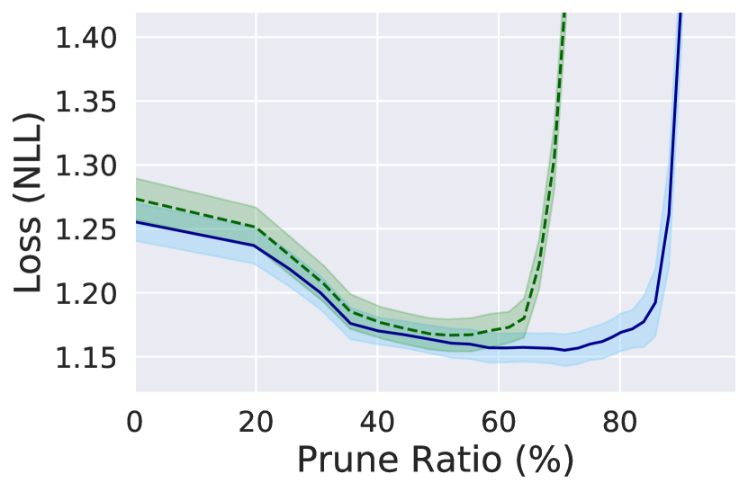
(a) Gaussians

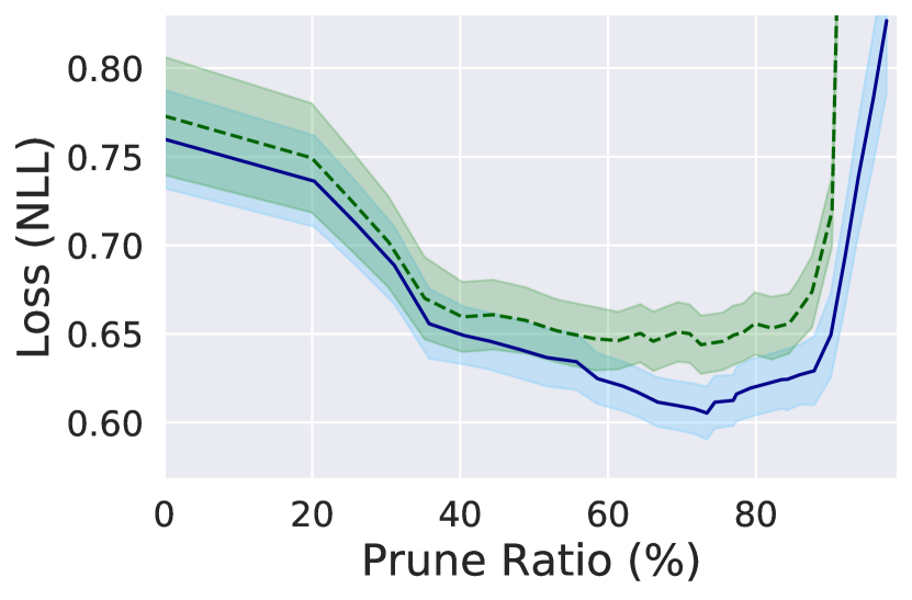
(b) Gaussian Spiral

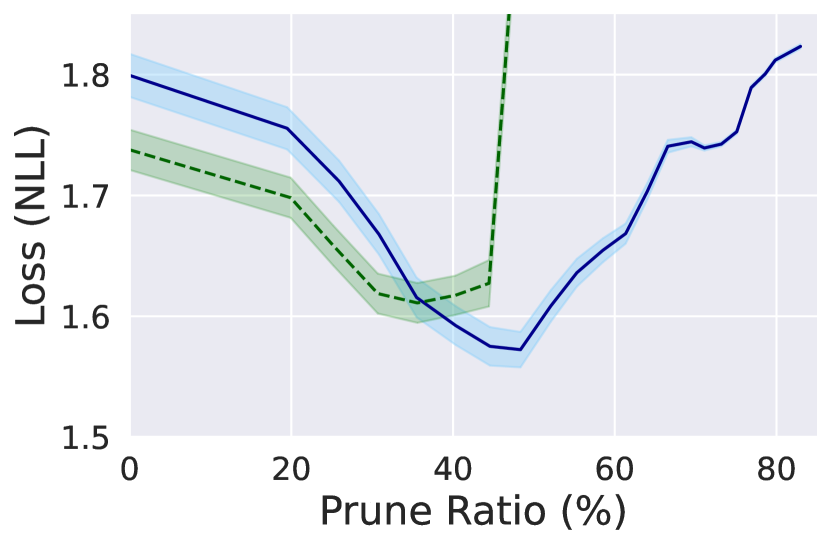
(c) Spiral

Figure 4: Negative log likelihood of Sparse Flow as function of prune ratio. In general, structured pruning is a more constrained problem as we constrain the type of sparsity. Hence, for almost any pruning experiment we can expect that structured pruning performs worse than unstructured pruning starting at a certain prune ratio.

Figure 5: Pruning FFJORD (PR= Prune ratio).

4.1 Density Estimation on 2D Data

In the first set of experiments, we train FFJORD on a multi-modal Gaussian distribution, a multi-model set of Gaussian distributions placed orderly on a spiral as well as a spiral distribution with sparse regions. Figure 5 (first row) illustrates that densely connected flows (prune ratio = 0%) might get stuck in sharp local minima and as a result induce mode collapse (Srivastava et al., 2017a). Once we perform unstructured pruning, we observe that the quality of the density estimation in all tasks considerably improves, c.f. Figure 5 (second and third rows). If we continue sparsifying the flows, depending on the task at hand, the flows get disrupted again.

Therefore, there is a certain threshold for pruning flows required to avoid generative modeling issues such as mode-collapse in continuous flows. We validate this observation by plotting the negative log-likelihood loss as a function of the prune ratio in all three tasks with both unstructured and structured pruning. As shown in Figure 4, we confirm that sparsity in flows improves the performance of continuous normalizing flows.

We further explore the inner dynamics of the flows between unpruned and pruned networks on the multi-modal case, with the aim of understanding how pruning enhances density estimation performance. Figure 6 represents the vector-field constructed by each flow to model 6-Gaussians independently. We observe that sparse flows with PR of 70% attract the vector-field directions uniformly towards the mean of each Gaussian. In contrast, unpruned flows do not exploit this feature and contain converging vectors in between distributions. This is how the mode-collapse occurs.

Figure 6: Multi-modal Gaussian flow and pruning. We observe that Sparse Flows attract the vector-field directions uniformly towards the mean of each Gaussian distribution, while an unpruned flow does not exploit this feature and contains converging vectors in between Gaussians. See Supplements Section S2, for a detailed explanation of these observations.

4.2 Density Estimation on Real Data - Tabular

We scale our experiments to a set of five real-world tabular datasets (prepared based on the instructions given by Papamakarios et al. (2017) and Grathwohl et al. (2019)) to verify our empirical observations about the effect of pruning on the generalizability of continuous normalizing flows. Table 2 summarizes the results. We observe that sparsifying FFJORD flows substantially improves their performance in all 5 tasks. In particular, we gain up to 42% performance gain in the POWER, 35% in GAS, 12% in HEPMASS, 5% in MINIBOONE and 19% in BSDS300.

More importantly, this is achieved with flows with 1 to 3 orders of magnitude less parameters compared to other advanced flows. On MINIBOONE dataset for instance, we found a sparse flow with only 4% of its original network that outperforms its densely-connected FFJORD flow. On MINIBOONE, Autoregressive flows (NAF) and sum-of-squares models (SOS) which outperform all other models possess 8.03 and 6.87 million parameters. In contrast, we obtain a Sparse Flow with only 32K parameters that outperform all models except NAF and SOS.

Table 2: Negative test log-likelihood (NLL) in nats of tabular datasets from (Papamakarios et al., 2017) and corresponding architecture size in number of parameters (#params). Sparse Flow (FFJORD with unstructured pruning) with lowest NLL and competing baseline with lowest NLL are bolded.

Model Power Gas Hepmass Miniboone BSDS300 nats #params nats #params nats #params nats #params nats #params MADE (Germain et al., 2015) 3.08 6K -3.56 6K 20.98 147K 15.59 164K -148.85 621K Real NVP (Dinh et al., 2016) -0.17 212K -8.33 216K 18.71 5.46M 13.84 5.68M -153.28 22.3M MAF (Papamakarios et al., 2017) -0.24 59.0K -10.08 62.0K 17.70 1.47M 11.75 1.64M -155.69 6.21M Glow (Kingma and Dhariwal, 2018) -0.17 N/A -8.15 N/A 18.92 N/A 11.35 N/A -155.07 N/A CP-Flow (Huang et al., 2020) -0.52 5.46M -10.36 2.76M 16.93 2.92M 10.58 379K -154.99 2.15M TAN (Oliva et al., 2018b) -0.60 N/A -12.06 N/A 13.78 N/A 11.01 N/A -159.80 N/A NAF (Huang et al., 2018) -0.62 451K -11.96 443K 15.09 10.7M 8.86 8.03M -157.73 42.3M SOS (Jaini et al., 2019) -0.60 212K -11.99 256K 15.15 4.43M 8.90 6.87M -157.48 9.09M FFJORD (Grathwohl et al., 2019) -0.35 43.3K -8.58 279K 17.53 547K 10.50 821K -128.33 6.70M Sparse Flow -0.45 30K -10.79 194K 16.53 340K 10.84 397K -145.62 4.69M -0.50 23K -11.19 147K 15.82 160K 10.81 186K -148.72 3.55M -0.53 13K -11.59 85K 15.60 75K 9.95 32K -150.45 2.03M -0.52 10K -11.47 64K 15.99 46K 10.54 18K -151.34 1.16M

Let us now look at the loss versus prune-ratio trends in all experiments to conclude our empirical observations on real-world tabular datasets. As shown in Figure 7, we observe that pruning considerably improves the performance of flows at larger scale as well.

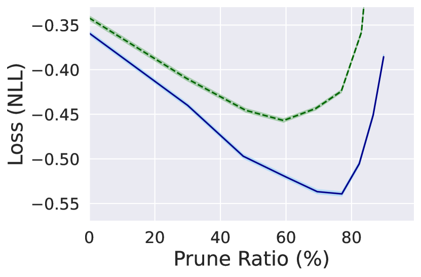
(a) Power

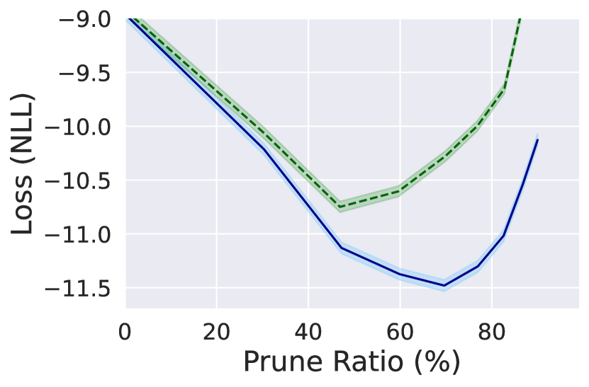
(b) Gas

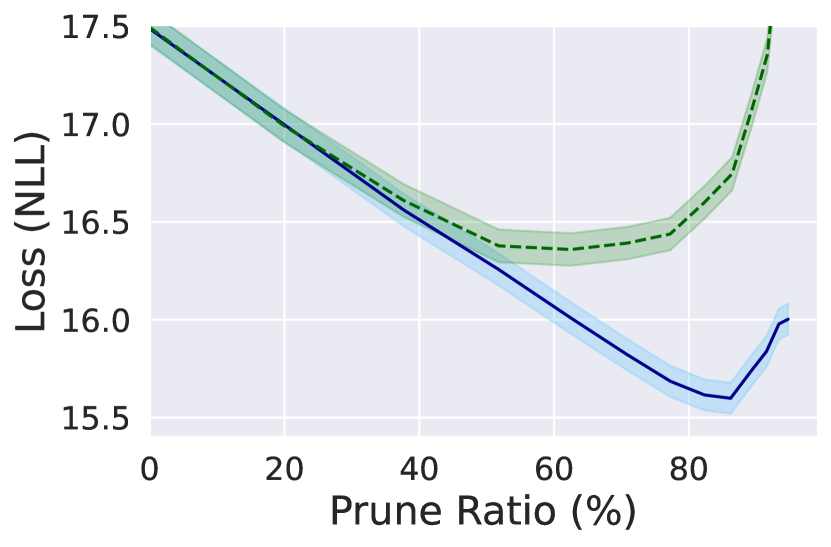
(c) Hepmass

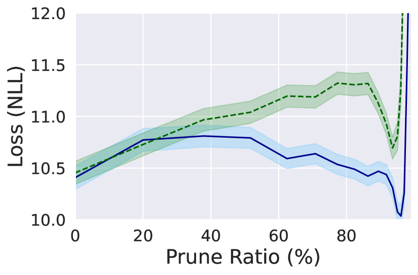
(d) Miniboone

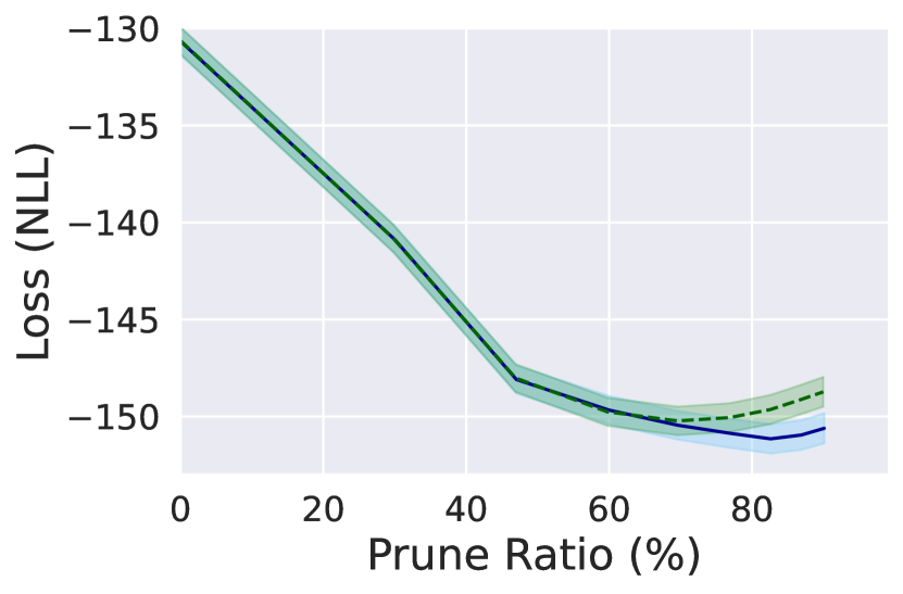
(e) Bsds300

Figure 7: Negative log-likelihood versus prune ratio on tabular datasets.

Table 3: Negative test log-likelihood (NLL) in bits/dim for image datasets and corresponding architecture size in number of parameters (#params). Sparse Flow (FFJORD with unstructured pruning) with lowest NLL and competing baseline with lowest NLL are bolded.

Model	MNIST		CIFAR-10
	bits/dim	#params	bits/dim	#params
MADE (Germain et al., 2015)	1.41	1.20M	5.80	11.5M
Real NVP (Dinh et al., 2016)	1.05	N/A	3.49	N/A
MAF (Papamakarios et al., 2017)	1.91	12.0M	4.31	115M
Glow (Kingma and Dhariwal, 2018)	1.06	N/A	3.35	44.0M
CP-Flow (Huang et al., 2020)	1.02	2.90M	3.40	1.90M
TAN (Oliva et al., 2018b)	1.19	N/A	3.98	N/A
SOS (Jaini et al., 2019)	1.81	17.2M	4.18	67.1M
RQ-NSF (Durkan et al., 2019)		N/A	3.38	11.8M
Residual Flow (Chen et al., 2019)	0.97	16.6M	3.28	25.2M
FFJORD (Grathwohl et al., 2019))	1.01	801K	3.44	1.36M
Sparse Flows (PR=20%)	0.97	641K	3.38	1.09M
Sparse Flows (PR=38%)	0.96	499K	3.37	845K
Sparse Flows (PR=52%)	0.95	387K	3.36	657K
Sparse Flows (PR=63%)	0.95	302K	3.37	510K
Sparse Flows (PR=71%)	0.96	234K	3.38	395K
Sparse Flows (PR=77%)	0.97	182K	3.39	308K
Sparse Flows (PR=82%)	0.98	141K	3.40	239K
Sparse Flows (PR=86%)	0.97	109K	3.42	186K

4.3 Density Estimation on Real Data - Vision

Next, we extend our experiments to density estimation for image datasets, MNIST and CIFAR10. We observe a similar case on generative modeling with both datasets, where pruned flows outperform densely-connected FFJORD flows. On MNIST, a sparse FFJORD flow with 63% of its weights pruned outperforms all other benchmarks. Compared to the second best flow (Residual flow), our sparse flow contains 70x less parameters (234K vs 16.6M). On CIFAR10, we achieve the second best performance with over 38x less parameters compared to Residual flows which performs best.

(a) MNIST

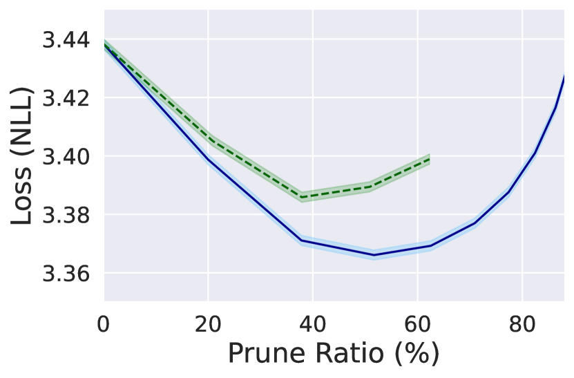
(b) CIFAR10

Figure 8: Loss vs. prune ratio for MNIST and CIFAR10 with unstructured and structured pruning.

Furthermore, on CIFAR10, Glow with 44 million parameters performs on par with our sparse FFJORD network with 657k parameters. It is worth mentioning that FFJORD obtains this results by using a simple Gaussian prior, while Glow takes advantage of learned base distribution (Grathwohl et al., 2019). Figure 8 illustrates the improvement of the loss (negative log-likelihood) in density estimation on image datasets as a result of pruning neural ODEs. Around 60% sparsity of a continuous normalizing flow leads to better generative modeling compared to densely structured flows.

4.4 Pruning Helps Avoid Mode-collapse

To quantitatively explore the effectiveness of pruning on avoiding mode-collapse (as shown qualitatively in Figure 5, we developed a measure adopted from (Srivastava et al., 2017b): The percentage of Good Quality samples— We draw samples from a trained normalizing flow and consider a sample of “good quality” if it is within $n$ ($n$ is typically chosen to be 2, 3, or 5) standard deviations from its nearest mode. We then can report the percentage of the good quality samples as a measure of how well the generative model captures modes.

Table 4 summarizes the results on some synthetic datasets and the large-scale MNIST dataset. We can see that the number of “good quality samples”, which stand for a quantitative metric for mode-collapse, improves consistently with a certain percentage of pruning in all experiments. This observation is very much aligned with our results on the generalization loss, which we will discuss in the following.

Table 4: Percentage of good quality samples as a measure of mode-collapse. Pruning method: structured pruning.

	Gaussian		Gaussian-spiral		MNIST
	Percentage of good quality samples as a measure of mode-collapse
Prune ratio (%)	std = 2	std = 3	std = 2	std = 3	Prune ratio (%)	std = 3	std = 5
0.0	72.89%	89.34%	66.65%	84.01%	0.0	6.94%	58.24%
20.0	79.46%	93.45%	74.29%	90.64%	20.0	8.02%	65.98%
25.6	81.40%	94.90%	78.22%	93.02%	37.8	9.35%	68.11%
52.0	84.30%	96.85%	80.40%	94.29%	51.7	8.70%	67.24%
71.2	81.83%	94.86%	78.06%	93.41%	77.3	8.59%	66.24%
75.1	68.20%	86.10%	78.99%	93.67%	89.3	6.07%	57.28%
98.0	36.01%	76.54%	9.27%	20.32%	91.7	0.02%	32.75%

4.5 Pruning Flattens the Loss Surface for Neural ODEs

What could be the potential reason for the enhanced generalization of pruned CNFs besides their ability to resolve mode-collapse? To investigate this further, we conducted a Hessian-based analysis on the flows-under-test. Dissecting the properties of the Hessian by Eigenanalysis allows us to gain useful insights about the behavior of neural networks (Hochreiter and Schmidhuber, 1997, Sagun et al., 2017, Ghorbani et al., 2019, Erichson et al., 2021, Lechner and Hasani, 2020). We use PyHessian (Yao et al., 2020) tool-set to analyze the Hessian $H$ w.r.t. the parameters of the CNF. This enables us to study the curvature of the loss function as the eigenvalues of the Hessian determines (locally) the loss gradients’ changes.

Table 5: Eigenanalysis of the Hessian $H$ in terms of the largest eigenvalue ($\lambda_{max}$), trace (tr), and condition number ($\kappa$) of pruned and unpruned continuous normalizing flows on the mixture of Gaussian task. Numbers are normalized with respect to the unpruned flow. See more results on other datasets in the supplements Section S3.

Model	NLL	$\lambda_{max}(H)$	$\text{tr}(H)$	$\kappa(H)$
Unpruned FFJORD	1.309	1.000	1.000	1.000
Sparse Flows (PR=20%)	1.163	0.976	0.858	0.825
Sparse Flows (PR=60%)	1.125	0.356	0.583	0.717
Sparse Flows (PR=70%)	1.118	0.295	0.340	0.709
Sparse Flows(PR=90%)	1.148	0.416	0.366	0.547

Larger Hessian eigenvalues therefore, stand for sharper curvatures and their sign identifies upward or downward curvatures. In Table 5, we report the maximum eigenvalue of the Hessian $\lambda_{max}$, Hessian’s Trace, and the condition number $\kappa=\frac{\lambda_{max}}{\lambda_{min}}$. Smaller $\lambda_{max}$ and tr($H$) indicates that our normalizing flow found a flatter minimum. As shown in Figure 3, a flat minimum leads to a better generalization error as opposed to a sharp minimum. We find that up to a certain prune ratio, the maximum of the Hessian decreases and increases thereafter. Therefore, we claim that pruned continuous flows finds flatter local minimum, therefore, it generalize better than their unpruned version.

Moreover, the Hessian condition number $\kappa$ could be an indicator of the robustness and efficiency of a deep model (Bottou and Bousquet, 2008). Smaller $\kappa$ corresponds to obtaining a more robust learned agent. We observe that $\kappa$ also follows the same trend and up to a certain prune ratio it shrinks and then increases again confirming our hypothesis.

4.6 On the Robustness of Decision Boundaries of Pruned ODE-based Flows

While pruning improves performance, it is imperative to investigate their robustness properties in constructing decision boundaries (Lechner et al., 2021). For feedforward deep models it was recently shown that although pruned networks perform as well as their unpruned version, their robustness significantly decreases due to smaller network size (Liebenwein et al., 2021a). Is this also the case for neural ODEs?

Figure 9: Robustness of decision boundaries for pruned networks. Column 1 is the decision boundary. Column 2 = state-space, and column 3 = the flow of data points: it shows the evolution of single samples (each narrow line represents an individual sample’s dimension 1 path) from input to their output through the depth of the network. How does the attenuation of the vector field intensity indicate that the classification boundary is more sensitive to perturbations? Let’s look at the first column and row 3 entry: We see that the classification boundary between the blue half-moon and the orange half-moon is very close to one tail of the blue half-moon. This means that if we perturb the blue half-moon data, some of them might get classified incorrectly based on the extremely pruned network’s decision boundary. As the intensity of the vector field shrinks to the center of the vector field (it is attenuated in the areas distant from the center), the decision boundary is set poorly as opposed to networks with more parameters.

We design an experiment to investigate this. We take a simple 2-Dimensional moon dataset and perform classification using unpruned and pruned neural ODEs. This experiment (shown in Figure 9) demonstrates another valuable property of neural ODEs: We observe that neural ODE instances pruned up to 84%, manage to establish a safe decision boundary for the two half moon classes. This insight about neural ODEs which was obtained by our pruning framework is another testimony of the merits of using neural ODE in decision-critical applications. Additionally, we observe that the decision-boundary gets very close to one of the classes for a network pruned up to 96% which reduces robustness. Though even this network instance provide the same classification accuracy compared to the densely connected version.

The state-space plot illustrates that a neural ODE’s learned vector-field becomes edgier as we keep pruning the network. Nonetheless, we observe that the distribution of the vector-field’s intensity (the color map in the second column) get attenuated as we go further away from its center, in highly pruned networks. This indicates that classification near the decision boundary is more sensitive to perturbations in extremely pruned networks.

Moreover, Column 3 of Figure 9 shows that when the networks are not pruned (column 3, row 1) or are pruned up to a certain threshold (column 3, row 2), the separation between the flow of samples of each class (orange or blue) is more consistent compared to the very pruned network (column 3, row 3). In Column 3, row 3 we see that the flow of individual samples from each class is more dispersed. As a result, the model is more sensitive to perturbations on the input space. This is very much aligned with our observation from column 1 and column 2 of Figure 9.

5 Discussions, Scope and Conclusions

We showed the effectiveness of pruning for continuous neural networks. Pruning improved generalization performance of continuous normalizing flows in density estimation tasks at scale. Additionally, pruning allows us to obtain performant minimal network instances with at least one order of magnitude less parameter count. By providing key insights about how pruning improves generative modeling and inference, we enabled the design of better neural ODE instances.

Ensuring sparse Hessian computation for sparse continuous-depth models. As we prune neural ODE instances, their weight matrices will contain zero entries. However the Hessian with respect to those zero entries is not necessarily zero. Therefore, when we compute the eigenvalues of the Hessian, we must ensure to make the decompositon vector sets the Hessian of the pruned weights to zero before performing our eigenanalysis.

Why experimenting with FFJORD and not CNFs? FFJORD is an elegant trick to efficiently compute the log determinant of the Jacobians in the change of variables formula for CNFs. Thus, FFJORDs are CNFs but faster. To confirm the effectiveness and scalability of our approach, we pruned some CNFs on toy datasets and concluded very similar outcomes (see these results in Appendix).

What are the limitations of Sparse Flows? Similar to any ODE-based learning system, the computational efficiency of sparse flows is highly determined by the choice of their ODE solvers, data and model parameters. As the complexity of any of these fronts increases, the number of function evaluations for a given task increases. Thus we might have a slow training process. This computational overhead can be relaxed in principle by the use of efficient ODE solvers (Poli et al., 2020b) and flow regularization schemes (Massaroli et al., 2020).

What design notes did we learn from applying pruning to neural ODEs? We performed an ablation study over different types of features of neural ODE models. These experiments can be found in the supplements Section S4. Our framework suggested that to obtain a generalizable sparse neural ODE representation, the choice of activation function is important. In particular activations that are Lipschitz continuous, monotonous, and bounded are better design choices for density estimation tasks.

Moreover, we found that the generalizability of sparse neural ODEs is more influenced by their neural network’s width than their depth (number of layers), c.f., Appendix Section S4. Furthermore, pruning neural ODEs allows us to obtain better hyperparameters for the optimization problem by setting a trade-off between the value of the learning rate and weight decay.

In summary, we hope to have shown compelling evidence for the effectiveness of having sparsity in ODE-based flows.

Lucas Liebenwein^∗
MIT CSAIL
lucas@csail.mit.edu
&Ramin Hasani^∗
MIT CSAIL
rhasani@mit.edu
&Alexander Amini
MIT CSAIL
amini@mit.edu
&Daniela Rus
MIT CSAIL
rus@csail.mit.edu

Supplementary Material

S1 Hyperparameters

We provide the necessary hyperparameters to reproduce our experiments below. For each set of experiments (Toy, Tabular, Images) we summarize the architecture of the unpruned model and relevant hyperparameters pertaining to the training/pruning process. All experiments were repeated three times with separate random seeds and average results are reported.

Table S1: Toy Dataset Hyperparameters.

Hyperparameters Gaussians GaussianSpiral Spiral Moon Architecture Layers 2 4 4 2 Hidden Size 128 64 64 128 Activation Sigmoid Sigmoid Sigmoid Tanh Divergence Hutchison Hutchison Hutchison Hutchison Solver Type Dopri Dopri Dopri Dopri Rel. tol. 1.0e-5 1.0e-5 1.0e-5 1.0e-4 Abs. tol 1.0e-5 1.0e-5 1.0e-5 1.0e-4 Backprop. Adjoint Adjoint Adjoint Adjoint (Re-)Training Optimizer AdamW AdamW AdamW Adam Epochs 100 100 100 50 Batch size 1024 1024 1024 128 LR 5.0e-3 5.0e-2 5.0e-2 1.0e-2 $\beta_{1}$ 0.9 0.9 0.9 0.9 $\beta_{2}$ 0.999 0.999 0.999 0.999 Weight decay 1.0e-5 1.0e-2 1.0e-6 1.0e-4 Pruning $PR$ 10% 10% 10% 10%

Table S2: Tabular Datasets Hyperparameters.

Hyperparameters Power Gas Hepmass Miniboone Bsds300 Architecture Please refer to Table 4, Appendix B.1 of Grathwohl et al. (2019). Solver Please refer to Appendix C of Grathwohl et al. (2019). (Re-)Training Optimizer Adam Adam Adam Adam Adam Epochs 100 30 400 400 100 Batch size 10000 1000 10000 1000 10000 LR 1.0e-3 1.0e-3 1.0e-3 1.0e-3 1.0e-3 LR step 0.1@{90, 97} 0.1@{25, 28} 0.1@{250, 295} 0.1@{300, 350} 0.1@{96, 99} $\beta_{1}$ 0.9 0.9 0.9 0.9 0.9 $\beta_{2}$ 0.999 0.999 0.999 0.999 0.999 Weight decay 1.0e-6 1.0e-6 1.0e-6 1.0e-6 1.0e-6 Pruning $PR$ 25% 25% 22% 22% 25%

Table S3: Image Datasets Hyperparameters.

Hyperparameters MNIST CIFAR-10 Architecture Please refer to Appendix B.1 (multi-scale) of Grathwohl et al. (2019). Solver Please refer to Appendix C of Grathwohl et al. (2019). (Re-)Training Optimizer Adam Adam Epochs 50 50 Batch size 200 200 LR 1.0e-3 1.0e-3 LR step 0.1@{45} 0.1@{45} $\beta_{1}$ 0.9 0.9 $\beta_{2}$ 0.999 0.999 Weight decay 0.0 0.0 Pruning $PR$ 22% 22%

S2 Figure 6 Clarifications

In figure below, we show the distribution and vector field of learned FFJORD networks (unpruned (top) and 70% pruned down). The area in the vector field declared with a black circle shows the vector field structure around an actual mode in the dataset. We see that the vector field (which is illustrated by black arrows) attracts samples towards the mean of this distribution in both pruned and unpruned networks.

However, there is a drastic difference between the vector field structure in-between modes (annotated by purple circles), between the unpruned and pruned network. In the unpruned network, the vector field attracts samples in-between modes. In contrast, in the pruned network, the vector field is repellent in-between modes. Correspondingly, this illustration shows how an unpruned network tends to have samples in-between modes, while the pruned network avoids this shortcoming.

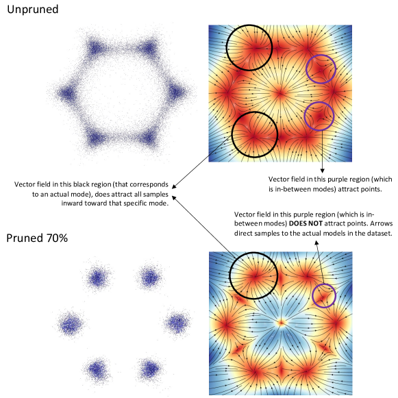
Figure S1: Clarification of how unpruned networks led to mode-collapse and pruned networks did not.

S3 Density Estimation on 2D Data with regular CNF

FFJORD is an efficient way to reparameterize continuous normalizing flows (CNFs) during the backwards pass in order to avoid computing the full Hessian, which can be prohibitively expensive in large-scale experiments. In this section, we validate whether our observations hold independent of the method to compute the Hessian.

Specifically, we train regular CNFs with full Hessian computation on a multi-modal Gaussian distribution, a multi-model set of Gaussian distributions placed orderly on a spiral as well as a spiral distribution with sparse regions following the setup from Section 4.1.

Figure S2 illustrates that densely connected flows (prune ratio = 0%) might get stuck in sharp local minima and thus exhibit unfavorable generalization performance in terms of the NLL. Once we perform pruning, we observe that the quality of the density estimation in all tasks considerably improves. If we continue sparsifying the flows, depending on the task at hand, the flows get disrupted again. Notably, we find that the straightforward Hessian computation may lead to slight improvements compared to using the FFJORD approximation, cf. results for the Spiral dataset using FFJORD and regular CNF as shown in Figure 4(c) and S2(c), respectively. This may be expected in certain cases as FFJORD replaces the exact Hessian computation with an approximation, thus potentially destabilizing training.

Overall, we can experimentally validate that our observations hold regardless of the specific method to compute the Hessian.

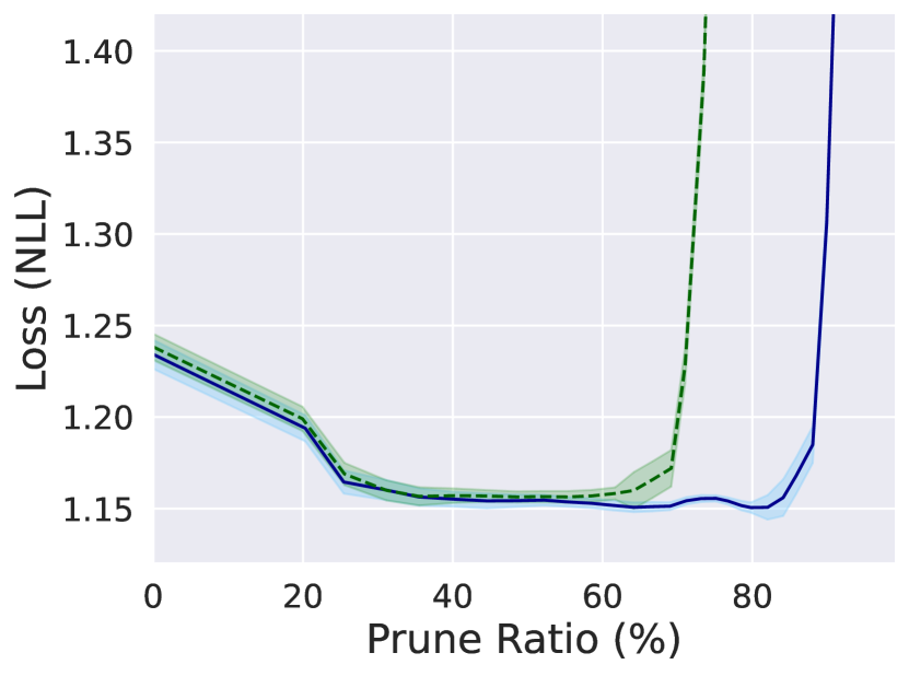
(a) Gaussians

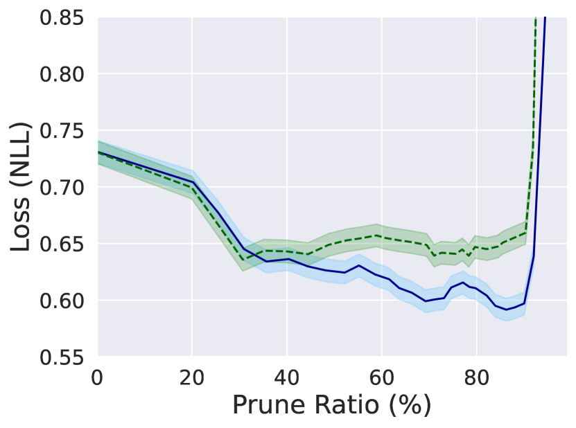
(b) Gaussian Spiral

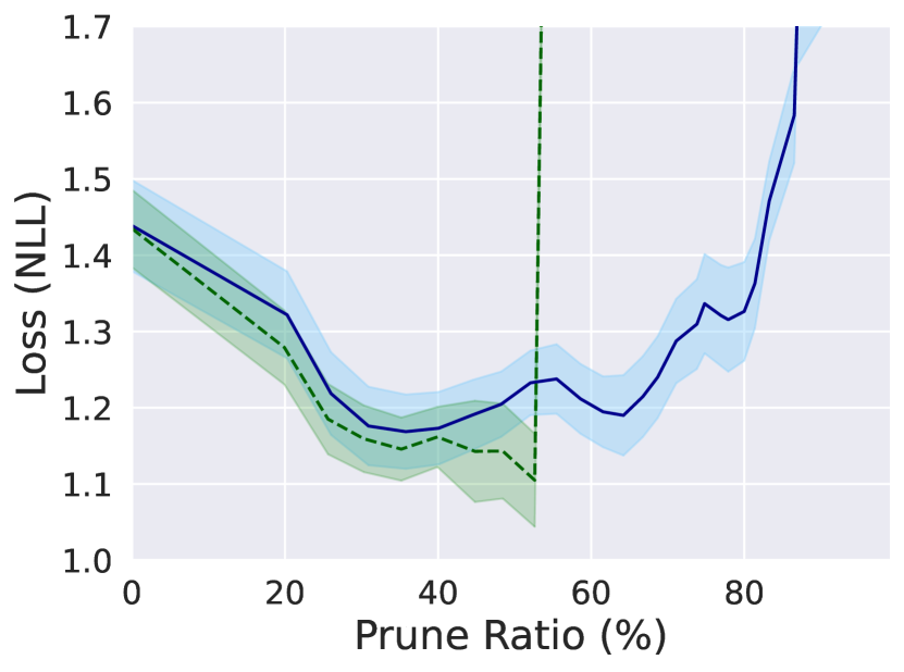
(c) Spiral

Figure S2: Negative log likelihood of Sparse Flow as function of prune ratio. Sparse Flows were trained using regular CNFs instead of the FFJORD approximation. The remaining experimental setup follows Section 4.1.

S4 Tabularized Results for Density Estimation on Real Data - Tabular

Table S4: Negative test log-likelihood (NLL) in nats on Power tabular dataset and corresponding architecture size in number of parameters and prune ratio for Sparse Flow (based on FFJORD). Results for unstructured and structured pruning are reported.

Power		Loss (nats)
Prune ratio (%)	Number of parameters	Unstructured	Structured
0%	43.3K	-0.34	-0.34
30%	30.3K	-0.48	-0.41
47%	23.0K	-0.50	-0.48
60%	17.4K	-0.51	-0.45
70%	13.2K	-0.55	-0.45
77%	9.95K	-0.55	-0.44
82%	7.65K	-0.52	-0.39
87%	5.81K	-0.45	-0.25
90%	4.43K	-0.39	0.04

Table S5: Negative test log-likelihood (NLL) in nats on Gas tabular dataset and corresponding architecture size in number of parameters and prune ratio for Sparse Flow (based on FFJORD). Results for unstructured and structured pruning are reported.

Gas		Loss (nats)
Prune ratio (%)	Number of parameters	Unstructured	Structured
0%	279K	-8.64	-8.64
30%	194K	-10.85	-10.63
47%	147K	-11.15	-10.93
60%	112K	-11.39	-10.69
70%	84.6K	-11.59	-10.20
77%	64.3K	-11.47	-9.95
83%	48.6K	-10.85	-9.85
87%	36.9K	-10.73	-9.16
90%	28.0K	-10.03	-7.58

Table S6: Negative test log-likelihood (NLL) in nats on Hepmass tabular dataset and corresponding architecture size in number of parameters and prune ratio for Sparse Flow (based on FFJORD). Results for unstructured and structured pruning are reported.

Hepmass		Loss (nats)
Prune ratio (%)	Number of parameters	Unstructured	Structured
0%	547K	17.54	17.54
20%	437K	16.90	16.91
38%	340K	16.56	16.54
52%	264K	16.22	16.39
63%	205K	16.00	16.21
71%	160K	15.80	16.48
77%	124K	15.67	16.48
82%	96.7K	15.58	16.35
86%	75.5K	15.59	16.97
89%	59.0K	15.62	16.92
92%	46.4K	15.99	17.34
93%	36.3K	15.90	17.80
95%	28.9K	16.04	18.77

Table S7: Negative test log-likelihood (NLL) in nats on Miniboone tabular dataset and corresponding architecture size in number of parameters and prune ratio for Sparse Flow (based on FFJORD). Results for unstructured and structured pruning are reported.

Miniboone		Loss (nats)
Prune ratio (%)	Number of parameters	Unstructured	Structured
0%	821K	10.38	10.38
20%	656K	10.83	10.87
38%	510K	11.11	10.93
52%	397K	10.50	11.09
62%	308K	10.77	11.10
71%	240K	10.51	11.40
77%	186K	10.64	11.07
82%	145K	10.46	11.50
86%	112K	10.37	11.35
89%	86.9K	10.44	11.11
92%	67.7K	10.60	10.93
94%	52.4K	10.27	10.75
95%	40.8K	10.05	10.41
96%	32.3K	9.90	11.26
97%	24.4K	10.15	12.09
98%	17.6K	10.72	14.92
99%	9.13K	13.61	39.01

Table S8: Negative test log-likelihood (NLL) in nats on Bsds300 tabular dataset and corresponding architecture size in number of parameters and prune ratio for Sparse Flow (based on FFJORD). Results for unstructured and structured pruning are reported.

Power		Loss (nats)
Prune ratio (%)	Number of parameters	Unstructured	Structured
0%	6.70M	-128.32	-128.32
30%	4.69M	-145.54	-145.42
47%	3.55M	-148.78	-148.70
60%	2.68M	-149.96	-149.92
70%	2.03M	-150.28	-150.66
77%	1.54M	-151.11	-150.11
83%	1.16M	-151.22	-149.41
87%	878K	-151.13	-149.42
90%	662K	-150.53	-148.59

S5 Tabularized Results for Density Estimation on Real Data - Vision

Below, we report the tabularized results on MNIST and CIFAR10 for Sparse Flow using unstructured and structured pruning. Note that highly sparse networks can fail to converge beyond a certain prune ratio. Moreover, structured pruning may not converge for lower prune ratios compared to unstructured pruning since we prune away entire channels and neurons in the former.

Table S9: Negative test log-likelihood (NLL) in bits/dim on MNIST and corresponding architecture size in number of parameters and prune ratio for Sparse Flow (based on FFJORD). Results for unstructured and structured pruning are reported.

MNIST		Loss (bits/dim)
Prune ratio (%)	Number of parameters	Unstructured	Structured
0%	801K	1.01	1.01
20%	641K	0.97	0.98
38%	499K	0.96	0.97
52%	387K	0.95	0.97
62%	302K	0.95	0.97
71%	234K	0.96	0.98
77%	182K	0.97	0.98
82%	141K	0.98	0.99
86%	109K	0.97	0.99
89%	84.5K	0.98	1.00

Table S10: Negative test log-likelihood (NLL) in bits/dim on CIFAR10 and corresponding architecture size in number of parameters and prune ratio for Sparse Flow (based on FFJORD). Results for unstructured and structured pruning are reported. “N/A” indicates that Sparse Flow did not converge for the given prune ratio.

CIFAR10		Loss (bits/dim)
Prune ratio (%)	Number of parameters	Unstructured	Structured
0%	1.36M	3.45	3.45
20%	1.09M	3.38	3.39
38%	845K	3.37	3.38
52%	657K	3.36	3.39
63%	510K	3.37	3.40
71%	395K	3.38	N/A
77%	308K	3.39	N/A
82%	239K	3.40	N/A
86%	186K	3.42	N/A
89%	144K	3.43	N/A
92%	112K	3.45	N/A
94%	86.7K	3.48	N/A
95%	67.4K	3.50	N/A

S6 More Hessian Analysis

We performed the following additional Hessian experiments. We observe that our conclusions on the behavior of the Hessian is generalizable to other datasets as well.

Table S11: Gaussians - Hessian Analysis (Structured Pruning)

Model	NLL	$\lambda_{max}(H)$	$\text{tr}(H)$	$\kappa(H)$
Unpruned FFJORD	1.173	0.0190	0.098	48.2k
Sparse Flows(PR=25%)	1.157	0.0110	0.076	2.76k
Sparse Flows(PR=67%)	1.148	0.0090	0.560	15.17k
Sparse Flows(PR=82%)	1.120	0.0065	0.058	22.75k
Sparse Flows(PR=90%)	1.136	0.0035	0.033	4.70k
Sparse Flows(PR=94%)	1.173	0.0069	0.033	3.94k
Sparse Flows(PR=96%)	1.244	0.0071	0.043	0.58k

Table S12: Gaussians-Spiral - Hessian Analysis (Structured Pruning)

Model	NLL	$\lambda_{max}(H)$	$\text{tr}(H)$	$\kappa(H)$
Unpruned FFJORD	0.880	0.0130	0.121	0.34k
Sparse Flows(PR=25%)	0.692	0.0076	0.058	0.76k
Sparse Flows(PR=48%)	0.634	0.0049	0.047	0.22k
Sparse Flows(PR=67%)	0.646	0.0052	0.051	0.75k
Sparse Flows(PR=82%)	0.657	0.0053	0.053	1.69k
Sparse Flows(PR=94%)	0.740	0.0086	0.070	0.11k
Sparse Flows(PR=96%)	0.986	0.0100	0.095	0.23k

S7 Ablation Study

In our ablation we study different types of features of neural ODE models. We have prepared our systematic ablation study with results provided as part of the supplementary material in the proceedings available here: https://openreview.net/forum?id=_1VZo_-aUiT.

Please find the detailed description of this ablation study in the README.txt file. We include this file’s description here as well.

Overview

We test different configurations by applying Sparse Flows (Algorithm 1) to investigate what type of network configurations are most stable and robust with respect to pruning. For each type of sweep (ablation), we highlight one key study and one key result.

Sweep over Optimization Parameters

Setup.

We study the stability of different configurations for the optimizer and how the different configurations affect the generalization performance during pruning.

Key observation.

We can find the most stable parameter configuration for the optimizer by considering sparsifying the flow and thus inducing additional regularization. The most stable optimizer configuration is the one for which we can achieve the most pruning.

Sweep over Model Sizes - Depth vs. Width

Setup.

We study different network configurations with (approximately) the same number of parameters. The networks differ in the depth vs. width configuration. We test deep and narrow vs. shallow and wide.

Key observation.

Increasing the depth of the network while reducing the width of the network, in general, does not help improve the generalization performance of the network over different prune ratios. Specifically, one should pick the minimal depth of the RHS that ensures convergence. Usually, any depth beyond that does not help improve the generalization performance of the flow.

Sweep over Activations

Setup.

We study the same network configurations for the same amount of pruning and vary the activation function of the neural network on the RHS. As we prune, we hope to unearth which activation function is most robust to pruning and consequently to changes in the architecture.

Key observation.

ReLU is usually not a very useful activation function. Rather, some Lipschitz continuous activation functions are most useful. Generally, we found tanh and sigmoid to be most useful, although sigmoid was probably the most robust single configuration across all experiments

Sweep over ODE Solvers

Setup.

We study the same network configurations for the same amount of pruning and vary the ODE solver of the neural ODE flow. As we prune, we hope to unearth which solver is most robust to pruning and consequently to changes in the architecture.

Key observation.

Generally, we found adaptive step size solvers (dopri5) superior to fixed step size solvers (rk4, Euler). Moreover, we found backpropagation through time (BPTT) to be slightly more stable than the adjoint method. Interestingly enough, we could oftentimes only observe the differences between the robustness of the different solvers after we start pruning and sparsifying the flows.

S8 More on Pruning Configurations

Iterative learning rate rewinding: We use learning rate rewinding (LRR) which is a hyperparameter schedule for training/pruning/retraining of neural nets (Renda et al., 2020) (see Algorithm 1).

Pre-defined pruning threshold: We pick a desired prune ratio and prune the weights with the smallest magnitudes until we obtain it. The largest weight that is being pruned constitutes the pre-defined threshold for pruning.

What kinds of structures are being considered in structured pruning? We consider neurons in fully-connected layers and channels with their corresponding filters in convolutional layers for structured pruning. The corresponding pruning score is the norm of the neuron/channel weights as specified in Table 1.

S9 Reproducibility Matters

All code and data which contains the details of the hyperparameters used in all experiments are openly accessible online at: https://github.com/lucaslie/torchprune For the experiments on the toy datasets, we based our code on the TorchDyn library (Poli et al., 2020a). For the experiments on the tabular datasets and image experiments, we based our code on the official code repository of FFJORD (Grathwohl et al., 2019).

References

- Adams et al. (2018) Ryan P Adams, Jeffrey Pennington, Matthew J Johnson, Jamie Smith, Yaniv Ovadia, Brian Patton, and James Saunderson. Estimating the spectral density of large implicit matrices. arXiv preprint arXiv:1802.03451, 2018.
- Baykal et al. (2019a) Cenk Baykal, Lucas Liebenwein, Igor Gilitschenski, Dan Feldman, and Daniela Rus. Data-dependent coresets for compressing neural networks with applications to generalization bounds. In International Conference on Learning Representations, 2019a. URL https://openreview.net/forum?id=HJfwJ2A5KX.
- Baykal et al. (2019b) Cenk Baykal, Lucas Liebenwein, Igor Gilitschenski, Dan Feldman, and Daniela Rus. Sipping neural networks: Sensitivity-informed provable pruning of neural networks. arXiv preprint arXiv:1910.05422, 2019b.
- Berg et al. (2018) Rianne van den Berg, Leonard Hasenclever, Jakub M Tomczak, and Max Welling. Sylvester normalizing flows for variational inference. arXiv preprint arXiv:1803.05649, 2018.
- Bottou and Bousquet (2008) Léon Bottou and Olivier Bousquet. The tradeoffs of large scale learning. In J. Platt, D. Koller, Y. Singer, and S. Roweis, editors, Advances in Neural Information Processing Systems, volume 20. Curran Associates, Inc., 2008. URL https://proceedings.neurips.cc/paper/2007/file/0d3180d672e08b4c5312dcdafdf6ef36-Paper.pdf.
- Chen et al. (2019) Ricky T. Q. Chen, Jens Behrmann, David K Duvenaud, and Joern-Henrik Jacobsen. Residual flows for invertible generative modeling. In H. Wallach, H. Larochelle, A. Beygelzimer, F. d'Alché-Buc, E. Fox, and R. Garnett, editors, Advances in Neural Information Processing Systems, volume 32. Curran Associates, Inc., 2019. URL https://proceedings.neurips.cc/paper/2019/file/5d0d5594d24f0f955548f0fc0ff83d10-Paper.pdf.
- Chen et al. (2018) Tian Qi Chen, Yulia Rubanova, Jesse Bettencourt, and David K Duvenaud. Neural ordinary differential equations. In Advances in neural information processing systems, pages 6571–6583, 2018.
- Dinh et al. (2015) Laurent Dinh, David Krueger, and Yoshua Bengio. Nice: Non-linear independent components estimation. In International Conference on Learning Representations, 2015.
- Dinh et al. (2016) Laurent Dinh, Jascha Sohl-Dickstein, and Samy Bengio. Density estimation using real nvp. arXiv preprint arXiv:1605.08803, 2016.
- Dormand and Prince (1980) John R Dormand and Peter J Prince. A family of embedded runge-kutta formulae. Journal of computational and applied mathematics, 6(1):19–26, 1980.
- Dupont et al. (2019) Emilien Dupont, Arnaud Doucet, and Yee Whye Teh. Augmented neural odes. In Advances in Neural Information Processing Systems, pages 3134–3144, 2019.
- Durkan et al. (2019) Conor Durkan, Artur Bekasov, Iain Murray, and George Papamakarios. Neural spline flows. arXiv preprint arXiv:1906.04032, 2019.
- Erichson et al. (2021) N. Benjamin Erichson, Omri Azencot, Alejandro Queiruga, Liam Hodgkinson, and Michael W. Mahoney. Lipschitz recurrent neural networks. In International Conference on Learning Representations, 2021. URL https://openreview.net/forum?id=-N7PBXqOUJZ.
- Finlay et al. (2020) Chris Finlay, Jörn-Henrik Jacobsen, Levon Nurbekyan, and Adam M Oberman. How to train your neural ode. arXiv preprint arXiv:2002.02798, 2020.
- Frankle and Carbin (2019) Jonathan Frankle and Michael Carbin. The lottery ticket hypothesis: Finding sparse, trainable neural networks. In International Conference on Learning Representations, 2019. URL https://openreview.net/forum?id=rJl-b3RcF7.
- Germain et al. (2015) Mathieu Germain, Karol Gregor, Iain Murray, and Hugo Larochelle. Made: Masked autoencoder for distribution estimation. In Francis Bach and David Blei, editors, Proceedings of the 32nd International Conference on Machine Learning, volume 37 of Proceedings of Machine Learning Research, pages 881–889, Lille, France, 07–09 Jul 2015. PMLR. URL http://proceedings.mlr.press/v37/germain15.html.
- Ghorbani et al. (2019) Behrooz Ghorbani, Shankar Krishnan, and Ying Xiao. An investigation into neural net optimization via hessian eigenvalue density. In International Conference on Machine Learning, pages 2232–2241. PMLR, 2019.
- Grathwohl et al. (2019) Will Grathwohl, Ricky T. Q. Chen, Jesse Bettencourt, Ilya Sutskever, and David Duvenaud. Ffjord: Free-form continuous dynamics for scalable reversible generative models. International Conference on Learning Representations, 2019.
- Han et al. (2015a) Song Han, Huizi Mao, and William J. Dally. Deep compression: Compressing deep neural network with pruning, trained quantization and huffman coding. CoRR, abs/1510.00149, 2015a. URL http://arxiv.org/abs/1510.00149.
- Han et al. (2015b) Song Han, Jeff Pool, John Tran, and William J Dally. Learning both weights and connections for efficient neural networks. In Proceedings of the 28th International Conference on Neural Information Processing Systems-Volume 1, pages 1135–1143, 2015b.
- Hasani et al. (2020) Ramin Hasani, Mathias Lechner, Alexander Amini, Daniela Rus, and Radu Grosu. A natural lottery ticket winner: Reinforcement learning with ordinary neural circuits. In International Conference on Machine Learning, pages 4082–4093. PMLR, 2020.
- Hasani et al. (2021) Ramin Hasani, Mathias Lechner, Alexander Amini, Daniela Rus, and Radu Grosu. Liquid time-constant networks. Proceedings of the AAAI Conference on Artificial Intelligence, 35(9):7657–7666, May 2021.
- Hassibi and Stork (1993) Babak Hassibi and David G Stork. Second order derivatives for network pruning: Optimal brain surgeon. Morgan Kaufmann, 1993.
- Hinton et al. (2015) Geoffrey Hinton, Oriol Vinyals, and Jeff Dean. Distilling the knowledge in a neural network. arXiv preprint arXiv:1503.02531, 2015.
- Hochreiter and Schmidhuber (1997) Sepp Hochreiter and Jürgen Schmidhuber. Long short-term memory. Neural computation, 9(8):1735–1780, 1997.
- Huang et al. (2018) Chin-Wei Huang, David Krueger, Alexandre Lacoste, and Aaron Courville. Neural autoregressive flows. In Jennifer Dy and Andreas Krause, editors, Proceedings of the 35th International Conference on Machine Learning, volume 80 of Proceedings of Machine Learning Research, pages 2078–2087. PMLR, 10–15 Jul 2018. URL http://proceedings.mlr.press/v80/huang18d.html.
- Huang et al. (2020) Chin-Wei Huang, Ricky TQ Chen, Christos Tsirigotis, and Aaron Courville. Convex potential flows: Universal probability distributions with optimal transport and convex optimization. arXiv preprint arXiv:2012.05942, 2020.
- Hutchinson (1989) Michael F Hutchinson. A stochastic estimator of the trace of the influence matrix for laplacian smoothing splines. Communications in Statistics-Simulation and Computation, 18(3):1059–1076, 1989.
- Jaini et al. (2019) Priyank Jaini, Kira A Selby, and Yaoliang Yu. Sum-of-squares polynomial flow. In International Conference on Machine Learning, pages 3009–3018. PMLR, 2019.
- Keskar et al. (2017) Nitish Shirish Keskar, Jorge Nocedal, Ping Tak Peter Tang, Dheevatsa Mudigere, and Mikhail Smelyanskiy. On large-batch training for deep learning: Generalization gap and sharp minima. In 5th International Conference on Learning Representations, ICLR 2017, 2017.
- Kingma and Dhariwal (2018) Diederik P Kingma and Prafulla Dhariwal. Glow: generative flow with invertible 1 1 convolutions. In Proceedings of the 32nd International Conference on Neural Information Processing Systems, pages 10236–10245, 2018.
- Kingma et al. (2016) Diederik P Kingma, Tim Salimans, Rafal Jozefowicz, Xi Chen, Ilya Sutskever, and Max Welling. Improving variational inference with inverse autoregressive flow. arXiv preprint arXiv:1606.04934, 2016.
- Kong and Chaudhuri (2020) Zhifeng Kong and Kamalika Chaudhuri. The expressive power of a class of normalizing flow models. In International Conference on Artificial Intelligence and Statistics, pages 3599–3609. PMLR, 2020.
- Lechner and Hasani (2020) Mathias Lechner and Ramin Hasani. Learning long-term dependencies in irregularly-sampled time series. arXiv preprint arXiv:2006.04418, 2020.
- Lechner et al. (2020a) Mathias Lechner, Ramin Hasani, Alexander Amini, Thomas A Henzinger, Daniela Rus, and Radu Grosu. Neural circuit policies enabling auditable autonomy. Nature Machine Intelligence, 2(10):642–652, 2020a.
- Lechner et al. (2020b) Mathias Lechner, Ramin Hasani, Daniela Rus, and Radu Grosu. Gershgorin loss stabilizes the recurrent neural network compartment of an end-to-end robot learning scheme. In 2020 IEEE International Conference on Robotics and Automation (ICRA), pages 5446–5452. IEEE, 2020b.
- Lechner et al. (2021) Mathias Lechner, Ramin Hasani, Radu Grosu, Daniela Rus, and Thomas A Henzinger. Adversarial training is not ready for robot learning. arXiv preprint arXiv:2103.08187, 2021.
- LeCun et al. (1990) Yann LeCun, John S Denker, and Sara A Solla. Optimal brain damage. In Advances in neural information processing systems, pages 598–605, 1990.
- Li et al. (2016) Hao Li, Asim Kadav, Igor Durdanovic, Hanan Samet, and Hans Peter Graf. Pruning filters for efficient convnets. arXiv preprint arXiv:1608.08710, 2016.
- Li et al. (2020) Xuechen Li, Ting-Kam Leonard Wong, Ricky TQ Chen, and David Duvenaud. Scalable gradients for stochastic differential equations. In International Conference on Artificial Intelligence and Statistics, pages 3870–3882. PMLR, 2020.
- Liebenwein et al. (2020) Lucas Liebenwein, Cenk Baykal, Harry Lang, Dan Feldman, and Daniela Rus. Provable filter pruning for efficient neural networks. In International Conference on Learning Representations, 2020. URL https://openreview.net/forum?id=BJxkOlSYDH.
- Liebenwein et al. (2021a) Lucas Liebenwein, Cenk Baykal, Brandon Carter, David Gifford, and Daniela Rus. Lost in pruning: The effects of pruning neural networks beyond test accuracy. Proceedings of Machine Learning and Systems, 3, 2021a.
- Liebenwein et al. (2021b) Lucas Liebenwein, Alaa Maalouf, Oren Gal, Dan Feldman, and Daniela Rus. Compressing neural networks: Towards determining the optimal layer-wise decomposition. arXiv preprint arXiv:2107.11442, 2021b.
- Luo et al. (2017) Jian-Hao Luo, Jianxin Wu, and Weiyao Lin. Thinet: A filter level pruning method for deep neural network compression. In Proceedings of the IEEE international conference on computer vision, pages 5058–5066, 2017.
- Maalouf et al. (2021) Alaa Maalouf, Harry Lang, Daniela Rus, and Dan Feldman. Deep learning meets projective clustering. In International Conference on Learning Representations, 2021. URL https://openreview.net/forum?id=EQfpYwF3-b.
- Massaroli et al. (2020) Stefano Massaroli, Michael Poli, Jinkyoo Park, Atsushi Yamashita, and Hajime Asma. Dissecting neural odes. In 34th Conference on Neural Information Processing Systems, NeurIPS 2020. The Neural Information Processing Systems, 2020.
- Molchanov et al. (2019) P Molchanov, S Tyree, T Karras, T Aila, and J Kautz. Pruning convolutional neural networks for resource efficient inference. In 5th International Conference on Learning Representations, ICLR 2017-Conference Track Proceedings, 2019.
- Müller et al. (2019) Thomas Müller, Brian McWilliams, Fabrice Rousselle, Markus Gross, and Jan Novák. Neural importance sampling. ACM Transactions on Graphics (TOG), 38(5):1–19, 2019.
- Oliva et al. (2018a) Junier Oliva, Avinava Dubey, Manzil Zaheer, Barnabas Poczos, Ruslan Salakhutdinov, Eric Xing, and Jeff Schneider. Transformation autoregressive networks. In International Conference on Machine Learning, pages 3898–3907. PMLR, 2018a.
- Oliva et al. (2018b) Junier Oliva, Avinava Dubey, Manzil Zaheer, Barnabas Poczos, Ruslan Salakhutdinov, Eric Xing, and Jeff Schneider. Transformation autoregressive networks. In Jennifer Dy and Andreas Krause, editors, Proceedings of the 35th International Conference on Machine Learning, volume 80 of Proceedings of Machine Learning Research, pages 3898–3907. PMLR, 10–15 Jul 2018b. URL http://proceedings.mlr.press/v80/oliva18a.html.
- Onken et al. (2020) Derek Onken, Samy Wu Fung, Xingjian Li, and Lars Ruthotto. Ot-flow: Fast and accurate continuous normalizing flows via optimal transport. arXiv preprint arXiv:2006.00104, 2020.
- Papamakarios et al. (2017) George Papamakarios, Theo Pavlakou, and Iain Murray. Masked autoregressive flow for density estimation. arXiv preprint arXiv:1705.07057, 2017.
- Poli et al. (2020a) Michael Poli, Stefano Massaroli, Atsushi Yamashita, Hajime Asama, and Jinkyoo Park. Torchdyn: A neural differential equations library. arXiv preprint arXiv:2009.09346, 2020a.
- Poli et al. (2020b) Michael Poli, Stefano Massaroli, Atsushi Yamashita, Hajime Asama, Jinkyoo Park, et al. Hypersolvers: Toward fast continuous-depth models. Advances in Neural Information Processing Systems, 33, 2020b.
- Pontryagin (2018) Lev Semenovich Pontryagin. Mathematical theory of optimal processes. Routledge, 2018.
- Renda et al. (2020) Alex Renda, Jonathan Frankle, and Michael Carbin. Comparing fine-tuning and rewinding in neural network pruning. In International Conference on Learning Representations, 2020. URL https://openreview.net/forum?id=S1gSj0NKvB.
- Rezende and Mohamed (2015) Danilo Rezende and Shakir Mohamed. Variational inference with normalizing flows. In International Conference on Machine Learning, pages 1530–1538. PMLR, 2015.
- Rumelhart et al. (1986) David E Rumelhart, Geoffrey E Hinton, and Ronald J Williams. Learning representations by back-propagating errors. nature, 323(6088):533–536, 1986.
- Sagun et al. (2017) Levent Sagun, Utku Evci, V Ugur Guney, Yann Dauphin, and Leon Bottou. Empirical analysis of the hessian of over-parametrized neural networks. arXiv preprint arXiv:1706.04454, 2017.
- Srivastava et al. (2017a) Akash Srivastava, Lazar Valkov, Chris Russell, Michael U. Gutmann, and Charles Sutton. Veegan: Reducing mode collapse in gans using implicit variational learning. In I. Guyon, U. V. Luxburg, S. Bengio, H. Wallach, R. Fergus, S. Vishwanathan, and R. Garnett, editors, Advances in Neural Information Processing Systems, volume 30. Curran Associates, Inc., 2017a. URL https://proceedings.neurips.cc/paper/2017/file/44a2e0804995faf8d2e3b084a1e2db1d-Paper.pdf.
- Srivastava et al. (2017b) Akash Srivastava, Lazar Valkov, Chris Russell, Michael U Gutmann, and Charles Sutton. Veegan: Reducing mode collapse in gans using implicit variational learning. In Proceedings of the 31st International Conference on Neural Information Processing Systems, pages 3310–3320, 2017b.
- Teshima et al. (2020) Takeshi Teshima, Isao Ishikawa, Koichi Tojo, Kenta Oono, Masahiro Ikeda, and Masashi Sugiyama. Coupling-based invertible neural networks are universal diffeomorphism approximators. arXiv preprint arXiv:2006.11469, 2020.
- Vorbach et al. (2021) Charles Vorbach, Ramin Hasani, Alexander Amini, Mathias Lechner, and Daniela Rus. Causal navigation by continuous-time neural networks. arXiv preprint arXiv:2106.08314, 2021.
- Wehenkel and Louppe (2019) Antoine Wehenkel and Gilles Louppe. Unconstrained monotonic neural networks. arXiv preprint arXiv:1908.05164, 2019.
- Yang and Karniadakis (2020) Liu Yang and George Em Karniadakis. Potential flow generator with l2 optimal transport regularity for generative models. IEEE Transactions on Neural Networks and Learning Systems, 2020.
- Yang et al. (2017) Tien-Ju Yang, Yu-Hsin Chen, and Vivienne Sze. Designing energy-efficient convolutional neural networks using energy-aware pruning. In Proceedings of the IEEE Conference on Computer Vision and Pattern Recognition, pages 5687–5695, 2017.
- Yao et al. (2020) Zhewei Yao, Amir Gholami, Kurt Keutzer, and Michael W Mahoney. Pyhessian: Neural networks through the lens of the hessian. In 2020 IEEE International Conference on Big Data (Big Data), pages 581–590. IEEE, 2020.