Damping of the Franz-Keldysh oscillations in the presence of disorder

Abstract

Franz-Keldysh oscillations of the optical absorption in the presence of short-range disorder are studied theoretically. The magnitude of the effect depends on the relation between the mean-free path in a zero field and the distance between the turning points in electric field. Damping of the Franz-Keldysh oscillations by the disorder develops at high absorption frequency. Effect of damping is amplified by the fact that, that electron and hole are most sensitive to the disorder near the turning points. This is because, near the turning points, velocities of electron and hole turn to zero.

I Introduction

Application of electric field to an insulator modifies the shape of the absorption spectrum in two respects: (i) below-threshold part of the spectrum develops a tail which becomes more voluminous upon increasing the field; (ii) above-the-threshold part of the spectrum acquires an oscillating component with a period of oscillations gradually decreasing as the field is increased. This effect predicted by Franz and KeldyshFranz ; Keldysh more than 60 years ago was subsequently observed on a large number of bulk semiconductors, see e.g. Ref. bulk, .

Figure 1: (Color online) Schematic illustration of the above-the-gap electroabsorption in an insulator. Initital kinetic energies of electron and hole are $\hbar\Omega_{e}$ and $\hbar\Omega_{e}$, respectively. Franz-Keldysh oscillations reflect the interference of incident electron (hole) wave with a wave reflected at the corresponding turning point. Disorder, illustrated with dots, leads to the smearing of the interference pattern, and, consequently, to the smearing of the oscillations. It is crucial that patterns for electron and hole are smeared by scattering from different impurities.

Later, theoretical and experimental studies were extended to quantum wellsChemla ; Well and quantum wires.Wire ; Wire1 Less trivial is that Franz-Keldysh oscillations were observed in certain polymers,polymer ; polymer1 and recently, in nanotubes,nanotube ; nanotube1 nanocrystals,nanocrystal and perovskites.perovskite0 ; perovskite1 ; perovskite2 Polymers and perovskites are known to be highly disordered materials with carrier mobilitymobility $\sim 10~{}\text{cm}^{2}\cdot\text{V}^{-1}\cdot\text{s}^{-1}$. Then the question arises, how the inherent disorder in these materials affects the Franz-Keldysh effect. Apparently, the effect of an electric field on the tail part of the absorption spectrum is weakened by the disorder. This is because the disorder creates a tail of its own. Effect of disorder on the above-the-threshold oscillations is of a different physical origin. It is illustrated in Fig. 1. Upon absorption of a photon, electron and hole have kinetic energies $\hbar\Omega_{e}$ and $\hbar\Omega_{h}$, respectively. They get, subsequently, reflected at the points $\pm x_{t}$, shown in the figure, and interfere with incident waves. The resulting density pattern resembles a standing wave. Presence of impurities ”scrambles” the standing-wave pattern, leading to the suppression of the Franz-Keldysh oscillations. This suppression is studied theoretically in the present paper. Superficially, it is clear that, in order to distinguish between the weak and strong disorder limits, one has to compare $x_{t}$ to the mean free path, $l$. For a weak disorder one has $l\gg x_{t}$, so the oscillations are not affected. However, there is a nontrivial aspect to this picture, namely, upon approaching the corresponding turning points, $\pm x_{t}$, kinetic energies of electron and hole turn to zero. Thus, the local mean free paths decrease dramatically. This contributes to the suppression of the interference, and thus, to the damping of the oscillations.

II Smearing of the Franz-Keldysh oscillations by the disorder

Without the disorder, the oscillating part of the absorption coefficient of light with frequency, $\omega$, in the presence of electric field, $F$, is given by

$$A(\Omega)\propto\sin\left[c\left(\frac{\hbar\Omega}{E_{0}}\right)^{3/2}\right],$$ (1)

where $c$ is a constant, and $\hbar\Omega=\hbar\omega-E_{g}$, where $E_{g}$ is a band-gap. For equal masses of electron and hole one has $c=\frac{2^{5/2}}{3}$. Energy, $E_{0}$, in Eq. (1) is defined as

$$E_{0}=\left(\frac{\hbar^{2}F^{2}}{m}\right)^{1/3}.$$ (2)

It has a meaning of the characteristic electron energy in the field, $F$.

Our main result is that, in the presence of disorder, the spectrum $A(\Omega)$ is multiplied by a damping factor $\exp\big{[}-{{\cal L}(\Omega)}\big{]}$, where the function ${\cal L}\left(\Omega\right)$ is defined as

$${\cal L}\left(\Omega\right)=\frac{m\gamma}{\hbar^{2}F}\ln\left(\frac{\hbar\Omega}{E_{0}}\right).$$ (3)

Here $\gamma$ is the factor in the correlation relation,

$$\langle V(x)V(x^{\prime})\rangle=\gamma\delta(x-x^{\prime}),$$ (4)

of the disorder potential, $V(x)$. Disorder leads to a finite scattering time. For electron with energy, $E$, the golden-rule calculation of the scattering time yields

$$\frac{\hbar}{\tau(E)}=\frac{\gamma}{2}\left(\frac{2m}{\hbar^{2}E}\right)^{1/2}.$$ (5)

Expression in the square bracket is a 1D density of states. Upon approaching the turning point, kinetic energy of electron decreases, and, thus, the scattering time shortens. Decrease of velocity upon approaching the turning point leads to additional shortening of the mean free path.

$$l_{E}=\Big{(}\frac{2E}{m}\Big{)}^{1/2}\tau(E)=\frac{2\hbar^{2}}{m\gamma}E.$$ (6)

Note, that oscillating absorption Eq. (1) corresponds to the large-argument asymptote of the square of the Airy function. It applies for $\hbar\Omega\gg E_{0}$ when the argument of sine is big.

Physical meaning of the prefactor $\frac{m\gamma}{\hbar^{2}F}$ in Eq. (3) is the following. Energy scale $E_{0}$ comes from the distance $x_{F}\sim\frac{E_{0}}{F}$. From Eq. (4) it follows that the r.m.s. random potential within the distance $x_{F}$ can be estimated as $V(x_{F})\sim\left(\frac{\gamma}{x_{F}}\right)^{1/2}$. Then the prefactor in Eq. (3) can be cast in the form $\left(\frac{V(x_{F})}{E_{0}}\right)^{2}$.

III General expression for the absorption coefficient

The golden-rule expression for the absorption coefficient of light with frequency, $\omega$, is the following

$$A(\omega)$$

$$\propto\sum_{\mu,\nu}\Big{|}\int d{\bf r}\psi_{\mu}^{e}({\bf r})\left(\psi_{\nu}^{h}({\bf r})\right)^{\ast}\Big{|}^{2}\delta\Big{[}\hbar\Omega_{\mu}^{e}+\hbar\Omega_{\nu}^{h}-\left(\hbar\omega-E_{g}\right)\Big{]},$$ (7)

where $\psi_{\mu}^{e}({\bf r})$, $\psi_{\nu}^{h}({\bf r})$ are the eigenfunctions of the initial and final states, while $\hbar\Omega_{\mu}^{e}$ and $\hbar\Omega_{\nu}^{h}$ are the corresponding energies. Since the eigenfunctions carry information about the disorder, it is convenient to ”decouple” the $\delta$-function as follows

$$\delta\Big{(}\Omega_{\mu}^{e}+\Omega_{\nu}^{h}-\omega+\frac{E_{g}}{\hbar}\Big{)}=\int d\Omega_{1}\int d\Omega_{2}$$

$$\times\delta\left(\omega-\frac{E_{g}}{\hbar}-\Omega_{1}-\Omega_{2}\right)\delta\left(\Omega_{1}-\Omega_{\mu}^{e}\right)\delta\left(\Omega_{2}-\Omega_{\nu}^{h}\right),$$ (8)

and rewrite $A(\omega)$ in the form

$$A(\omega)=\int d\Omega_{1}\int d\Omega_{2}\delta\left(\Omega_{1}+\Omega_{2}+\frac{E_{g}}{\hbar}-\omega\right)$$

$$\times\int d{\bf r}_{1}\int d{\bf r}_{2}\text{Im}G_{e}({\bf r}_{1},{\bf r_{2}},\Omega_{1})\text{Im}G_{h}({\bf r}_{1},{\bf r_{2}},\Omega_{2}),$$ (9)

where the imaginary parts of the Green functions are defined as

$$\text{Im}G_{e}({\bf r}_{1},{\bf r}_{2},\Omega_{1})=\sum_{\mu}\psi_{\mu}^{e}({\bf r}_{1})\left(\psi_{\mu}^{e}({\bf r}_{2})\right)^{\ast}\delta\left(\Omega_{\mu}^{e}-\Omega_{1}\right),$$

$$\text{Im}G_{h}({\bf r}_{1},{\bf r}_{2},\Omega_{2})=\sum_{\nu}\left(\psi_{\nu}^{h}({\bf r}_{1})\right)^{\ast}\psi_{\nu}^{h}({\bf r}_{2})\delta\left(\Omega_{\nu}^{h}-\Omega_{2}\right).$$ (10)

In the presence of disorder, the product $\text{Im}G_{e}\text{Im}G_{h}$ in the right-hand side should be averaged over different configurations. It is crucial, that the disorder-induced smearing of the interference patterns for electrons and holes is dominated by different impurities. This is illustrated in Fig. 1. As a result, the disorder averaging can be performed independently.

IV Semiclassical calculation of the absorption damping in 1D

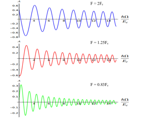
Figure 2: (Color online) Evolution of Franz-Keldysh oscillations with applied electric field is plotted from Eqs. (1) and (3) for three values of electric field, $F$, measured in the units of $F_{c}$ given by Eq. (21). Energy $\hbar\Omega$ is measured in the units of $E_{c}=\left(\frac{m\gamma^{2}}{2\hbar^{2}}\right)^{1/3}$.

Franz-Keldysh oscillations emerge in semiclassical regime, when electron and hole states can be described by local wave vectors

$$k_{e}(x)=\left(\frac{2m}{\hbar^{2}}\right)^{1/2}\left(\hbar\Omega_{1}-Fx\right)^{1/2},$$ (11)

$$k_{h}(x)=\left(\frac{2m}{\hbar^{2}}\right)^{1/2}\left(\hbar\Omega_{2}+Fx\right)^{1/2}.$$ (12)

In accordance with Fig. 1, $k_{e}(x)$ turns to zero at the right turning point, while $k_{h}(x)$ turns to zero at the left turning point. Electron and hole Green functions, which enter the light absorption Eq. (III) can be expressed in terms of $k_{e}(x)$ and $k_{h}(x)$ as follows

$$\text{Im}G_{e}^{(0)}(x_{1},x_{2},\Omega_{1})=\frac{\cos\left(\Phi_{e}(x_{1})-\frac{\pi}{4}\right)\cos\left(\Phi_{e}(x_{2})-\frac{\pi}{4}\right)}{\left(k_{e}(x_{1})k_{e}(x_{2})\right)^{1/2}},$$

$$\text{Im}G_{h}^{(0)}(x_{1},x_{2},\Omega_{2})=\frac{\cos\left(\Psi_{h}(x_{1})+\frac{\pi}{4}\right)\cos\left(\Psi_{h}(x_{2})+\frac{\pi}{4}\right)}{\left(k_{h}(x_{1})k_{h}(x_{2})\right)^{1/2}}.$$ (13)

where the semiclassical actions $\Phi_{e}$ and $\Phi_{h}$ are defined as

$$\Phi_{e}(x_{1})=\int\limits_{x_{1}}^{\hbar\Omega_{1}/F}dx^{\prime}k_{e}(x^{\prime}),~{}\Psi_{h}(x_{1})=\int\limits_{-\hbar\Omega_{2}/F}^{x_{1}}dx^{\prime}k_{h}(x^{\prime}).$$ (14)

Expressions Eq. (IV) are semiclassical and apply away from the turning points:

$$\Big{(}\frac{\hbar\Omega_{1}}{F}-x_{1}\Big{)}\gg\Big{(}\frac{\hbar^{2}}{mF}\Big{)}^{1/3}=x_{F},~{}\Big{(}x_{1}+\frac{\hbar\Omega_{2}}{F}\Big{)}\gg x_{F}.$$ (15)

Our goal is to incorporate disorder into the Green functions. For this purpose we transform the products of the cosines into the sums

$$\text{Im}G_{e}^{(0)}(x_{1},x_{2},\Omega_{1})$$

$$=\frac{\cos\left(\Phi_{e}(x_{1})-\Phi_{e}(x_{2})\right)+\cos\left(\Phi_{e}(x_{1})+\Phi_{e}(x_{2})-\frac{\pi}{2}\right)}{\left(k_{e}(x_{1})k_{e}(x_{2})\right)^{1/2}},$$ (16)

$$\text{Im}G_{h}^{(0)}(x_{1},x_{2},\Omega_{2})$$

$$=\frac{\cos\left(\Psi_{h}(x_{1})-\Psi_{h}(x_{2})\right)+\cos\left(\Psi_{h}(x_{1})+\Psi_{h}(x_{2})+\frac{\pi}{2}\right)}{\left(k_{h}(x_{1})k_{h}(x_{2})\right)^{1/2}}.$$ (17)

Physically, the first term in Eq. (IV) describes the propagation of electron from $x_{1}$ to $x_{2}$, while the second term describes the motion of electron from $x_{1}$ to the turning point, $x=x_{t}$ followed by reflection from the electrostatic barrier and return to $x_{2}$. It is shown in the Appendix in great detail that disorder averaging of the first term amounts to multiplying this term by $\exp(-|x_{2}-x_{1}|/l)$ when the mean free path, $l$, does not depend on $x$. Since, in electric field, kinetic energy of electron is a function of position, and $l$ is a function of energy, we conclude that the mean free path is a function of position. Then the natural generalization of the damping factor is $\exp\Big{(}-\int\limits_{x_{1}}^{x_{2}}\frac{dx}{l(x)}\Big{)}$. Substituting the $x$-dependent kinetic energy into Eq. (6), we get the following expressions for the mean free paths of electrons and holes

$$l_{1}(x)^{-1}=\frac{m\gamma}{2\hbar^{2}(\hbar\Omega_{1}-Fx)},~{}l_{2}(x)^{-1}=\frac{m\gamma}{2\hbar^{2}(\hbar\Omega_{2}+Fx)}.$$ (18)

Thus, incorporation of disorder into the Green functions $\text{Im}G_{e}^{(0)}(x_{1},x_{2})$ and $\text{Im}G_{h}^{(0)}(x_{1},x_{2})$ amounts to ascribing to each cosine in Eqs. (IV and (IV) its corresponding damping factor.

Turning to the product $\text{Im}G_{e}^{(0)}\text{Im}G_{h}^{(0)}$ we notice that the piece of this product that captures the Franz-Keldysh oscillations involves both the reflection of electron from electrostatic barrier at $x=x_{t}$ and reflection of hole from electrostatic barrier at $x=-x_{t}$. This process is encoded into the product

$$\cos\left(\Phi_{e}(x_{1})+\Phi_{e}(x_{2})-\frac{\pi}{2}\right)\cos\left(\Psi_{h}(x_{1})+\Psi_{h}(x_{2})+\frac{\pi}{2}\right)$$

$$=\frac{1}{2}\Bigg{[}-\cos\Big{(}\Phi_{e}(x_{1})-\Psi_{h}(x_{1})+\Phi_{e}(x_{2})-\Psi_{h}(x_{2})\Big{)}$$

$$+\cos\Big{(}\Phi_{e}(x_{1})+\Psi_{h}(x_{1})+\Phi_{e}(x_{2})+\Psi_{h}(x_{2})\Big{)}\Bigg{]}.$$ (19)

It is the second cosine that captures two reflections. The damping factor corresponding to this cosine has the form $\exp\left(-{\cal L}\right)$, where ${\cal L}$ is given by

$${\cal L}=\int\limits_{-\hbar\Omega_{2}/F}^{x_{1}}\frac{dx}{l_{h}(x)}+\int\limits_{x_{1}}^{\hbar\Omega_{1}/F}\frac{dx}{l_{e}(x)}+\int\limits_{-\hbar\Omega_{2}/F}^{x_{2}}\frac{dx}{l_{h}(x)}+\int\limits_{x_{2}}^{\hbar\Omega_{1}/F}\frac{dx}{l_{e}(x)}.$$ (20)

The remaining task is to substitute Eqs. (IV) and (20) into Eq. (III) and perform the integration over $\Omega_{1}$, $\Omega_{2}$, $x_{1}$, $x_{2}$. Integration is determined by rapidly changing cosine Eq. (IV). Concerning the damping factor, it is sufficient to substitute $\Omega_{1}=\Omega_{2}=\frac{E_{g}-\hbar\omega}{2\hbar}$ and set $x_{1}=x_{2}=0$. Integrals in Eq. (20) diverge logarithmically. A natural cutoff of the logarithms is $x_{F}$, see Eq. (15). Then Eq. (20) reduces to our main result Eq. (3).

V Concluding remarks

In traditional semiconductor materials the shape of the Franz-Keldysh oscillations is quite robust.Sipe Previous theoretical studiesexciton1 ; Aspnes ; Dow ; Merkulov ; Dow1 ; Aronov were focused on the effect of electron-hole attraction on electroabsorption. Numerical calculationsSipe indicate that the excitonic effect does not alter the shape of the oscillations. Rather, a smooth background on which Franz-Keldysh oscillations develop becomes more pronounced due to the electron-hole attraction.Sipe Effect of disorder on the oscillations is illustrated in Fig. 2, where the oscillations are plotted from Eqs. (1) and (3) for a given disorder and three values of electric field. It is seen that, while disorder damps the oscillations, this damping becomes less effective upon increasing, $F$. Physically, upon increasing $F$, the travel distance of electron and hole from the respective turning points to the point of their meeting becomes shorter. To estimate quantitatively the critical field, $F_{c}$, above which the effect of disorder becomes negligible, we express $F_{c}$ in terms of the width, $E_{c}$, of the tail in the density of states, which disorder creates in the absence of external field. The width, $E_{c}$, can be estimated by equating the uncertainty, $\frac{\hbar}{\tau(E_{c})}$, given by Eq. (5) to $E_{c}$. This yields $E_{c}=\left(\frac{\gamma}{2}\right)^{2/3}\left(\frac{2m}{\hbar^{2}}\right)^{1/3}$. Now the parameter $\gamma$ can be expressed via the observable $E_{c}$. Then, equating to one the prefactor, $\frac{m\gamma}{\hbar^{2}F}$, in front of logarithm in Eq. (3) yields the value

$$F_{c}=\frac{\left(mE_{c}^{3}\right)^{1/2}}{\hbar}.$$ (21)

For example, setting $m$ equal to the free electron mass, for disordered system with a tail $E_{c}=0.1~{}\text{eV}$, we conclude that Franz-Keldysh oscillations are smeared when the applied field is smaller than $1.5~{}\text{kV}\cdot\text{cm}^{-1}$. Note that, the tail, $E_{c}$, can be related to the mean free path $l_{c}=\left(\frac{\hbar^{2}}{mE_{c}}\right)^{1/2}\approx 10~{}\mathring{A}$. The above values are consistent with those reported for polymers.polymer ; polymer1 Overall, quantitative comparison of theoretical results with numerous experimental data is complicated by the fact that experimental papers do not list the values of electric field, but rather the voltage drop on the sample. Qualitatively though, experimental data on the Franz-Keldysh oscillations are in agreement with our prediction: Decrease of the oscillation period with their number is weak, while the visibility of high-order oscillations increases with increasing, $F$. To account for this effect, the authors of Refs. polymer, , polymer1, adopted a phenomenological approach: in calculation of absorption spectrum the electron energy, $E$, is replaced by $E+i\Gamma$, where parameter $\Gamma$ emulates the disorder. It is used as a fitting parameter. In this regard, within our theory, the role of “coherence length” in Refs. polymer, , polymer1, is played by the mean free path due to impurity scattering and depends strongly on, $F$. We have restricted consideration to the 1D case. The result in 2D does not differ qualitatively. This is because the electron travel path towards the turning point lies close to the travel path of the reflected electron. This is illustrated in Fig. 3. Quantitatively, the difference between the 2D and 1D cases is that the density of states in 2D is constant, so that the mean free path grows with energy slower, as $E^{1/2}$ rather than as $E$.

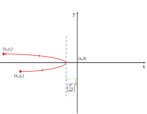
Figure 3: (Color online) Illustration of the Franz-Keldysh oscillations in 2D. Semiclassical trajectory of electron from the point $x_{1},y_{1}$ towards the electrostatic barrier is close to the trajectory from the barrier to the point $x_{2},y_{2}$. Electron, moving along the semiclassical trajectory is scattered by the disorder, which “scrambles” the interference pattern responsible for the oscillations.

Appendix A Average Green’s function near a wall

In the presence of a wall at $y=0$, the Green’s function of a free electron in the half-space $y>0$ has a form

$$G^{(0)}\left(E,y,y^{\prime}\right)=\frac{im}{\hbar^{2}k_{E}}\Big{[}e^{-ik_{E}|y-y^{\prime}|}-e^{-ik_{E}(y+y^{\prime})}\Big{]},$$ (22)

where $k_{E}=\left(\frac{2mE}{\hbar^{2}}\right)^{1/2}$ is a wave vector. The function $G^{(0)}$ satisfies the boundary conditions $G^{(0)}\left(E,0,y^{\prime}\right)=G^{(0)}\left(E,y,0\right)=0$.

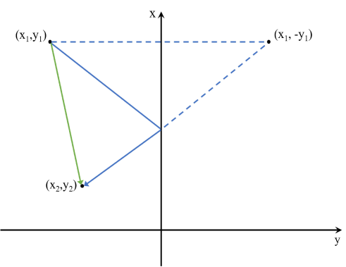
Figure 4: (Color online) Illustration of the 2D Green’s function in the presence of a wall at $y=0$. There are two classical paths between the points $(x_{1},y_{1})$ and $(x_{2},y_{2})$. One path is along the straight line, while the other path corresponds to the shortest classical trajectory reflected from the wall.

With a random disorder potential, $V(y)$, the Green’s function satisfies the Dyson equation

$$G(y_{1},y_{2})=G^{(0)}(y_{1},y_{2})+\int\limits_{0}^{\infty}dyG^{(0)}(y_{1},y)V(y)G(y,y_{2}).$$ (23)

This equation is exact. It can be cast into a different form upon substituting the right-hand side into the integrand

$$G(y_{1},y_{2})=G^{(0)}(y_{1},y_{2})+\int\limits_{0}^{\infty}dyG^{(0)}(y_{1},y)V(y)G^{(0)}(y,y_{2})$$

$$+\int\limits_{0}^{\infty}dy\int\limits_{0}^{\infty}dy^{\prime}G^{(0)}(y_{1},y)V(y)G^{(0)}(y,y^{\prime})V(y^{\prime})G(y^{\prime},y_{2}).$$ (24)

A crucial step which allows to get a closed equation for the average Green’s function is decoupling of averaging in the integrand of Eq. (A). Assuming that the potential $V(y)$ is short-ranged

$$\langle V(y)V(y^{\prime})\rangle=\gamma\delta(y-y^{\prime}),$$ (25)

and performing the averaging, we arrive to the closed RPA equation

$$\langle G(y_{1},y_{2})\rangle=G^{(0)}(y_{1},y_{2})$$

$$+\gamma\int\limits_{0}^{\infty}dyG^{(0)}(y_{1},y)G^{(0)}(y,y)\langle G(y,y_{2})\rangle.$$ (26)

In the absence of the wall, the bare Green’s function is equal to $G^{(0)}=\frac{im}{\hbar^{2}k_{E}}e^{-ik_{E}|y-y^{\prime}|}$ and the lower limit in the integral Eq. (A) should be set to $-\infty$. Then the average Green’s function depends only on the difference $(y_{1}-y_{2})$. This allows to solve Eq. (A) with the help of the Fourier transform. As a result, the disorder leads to a factor $\exp\big{(}-\frac{|y_{1}-y_{2}|}{l}\big{)}$ in the average Green’s function. Here $l$ is the mean free path which can be expressed via the disorder strength as follows

$$l=\frac{\hbar^{4}k_{E}^{2}}{m^{2}\gamma}.$$ (27)

The above result applies when the disorder is weak, namely, for $k_{E}l\gg 1$.

In the presence of the wall, the translational symmetry is violated. Taking the Fourier transform is not permissible. Yet, the form of the disorder-modified average Green’s function can be established from the following reasoning. The travel distance between the points $y_{1}$ and $y_{2}$ is either $|y_{1}-y_{2}|$, when the particle travels directly, or $(y_{1}+y_{2})$, when the travel involves the reflection from the wall. This suggests the following form

$$\langle G\left(E,y,y^{\prime}\right)\rangle$$

$$=\frac{im}{\hbar^{2}k_{E}}\Big{[}e^{-ik_{E}|y-y^{\prime}|}e^{-\frac{|y-y^{\prime}|}{l}}-e^{-ik_{E}(y+y^{\prime})}e^{-\frac{(y+y^{\prime})}{l}}\Big{]}.$$ (28)

of the average Green’s function.

A nontrivial question is a minimal distance at which Eq. (A) applies. We will show that the condition of applicability is $y_{1},y_{2}\gg\frac{1}{k_{E}}$.

To solve the equation Eq. (A) approximately, we make a substitution

$$\langle G(y,y^{\prime})\rangle$$

$$=\frac{im}{\hbar^{2}k_{E}}\Big{[}R_{1}(y,y^{\prime})e^{-ik_{E}|y-y^{\prime}|}-R_{2}(y,y^{\prime})e^{-ik_{E}(y+y^{\prime})}\Big{]},$$ (29)

and assume that $R_{1}$ and $R_{2}$ are slow functions on the scale $k_{E}^{-1}$. Substituting the form Eq. (A) into Eq. (A), we cast it into the form

$$\Big{(}R_{1}(y,y^{\prime})-1\Big{)}e^{-ik_{E}|y-y^{\prime}|}-\Big{(}R_{2}(y,y^{\prime})-1\Big{)}e^{-ik_{E}(y+y^{\prime})}$$

$$=\gamma\left(\frac{im}{\hbar^{2}k_{E}}\right)^{2}\int\limits_{0}^{\infty}dy_{1}\Big{(}e^{-ik_{E}|y-y_{1}|}-e^{-ik_{E}(y+y_{1})}\Big{)}\left(1-e^{-2ik_{E}y_{1}}\right)\Big{(}R_{1}(y_{1},y^{\prime})e^{-ik_{E}|y_{1}-y^{\prime}|}-R_{2}(y_{1},y^{\prime})e^{-ik_{E}(y_{1}+y^{\prime})}\Big{)}.$$ (30)

Without the loss of generality we assume that $y^{\prime}>y$. The key step is dividing the integral in the right-hand-side of Eq. (A) into three domains: (i) $0<y_{1}<y$, (ii) $y<y_{1}<y^{\prime}$, and (iii) $y_{1}>y^{\prime}$. Consider first the domain (i). In this domain, we have $|y-y_{1}|=y-y_{1}$, $|y_{1}-y^{\prime}|=y^{\prime}-y_{1}$. Out of six terms in the integrand only two terms, $-e^{-ik_{E}|y-y_{1}|}R_{2}(y_{1},y^{\prime})e^{-ik_{E}(y_{1}+y^{\prime})}=-e^{-ik_{E}(y+y^{\prime})}R_{2}(y_{1},y^{\prime})$, and $-e^{-ik_{E}y}R_{1}(y_{1},y^{\prime})e^{-ik_{E}y^{\prime}}=-e^{-ik_{E}(y+y^{\prime})}R_{1}(y_{1},y^{\prime})$ do not oscillate with $y_{1}$, since the functions $R_{1}$ and $R_{2}$ are slow. All other terms, e.g. $e^{-ik_{E}|y-y_{1}|}R_{1}(y_{1},y^{\prime})e^{-ik_{E}|y_{1}-y^{\prime}|}=e^{-ik_{E}(y+y^{\prime})}R_{1}(y_{1},y^{\prime})e^{2ik_{E}y_{1}}$, contain rapidly oscillating exponential factors. These factors suppress the integral over the domain (i) down to $k_{E}^{-1}$. Similar strategy is applied to the domains (ii) and (iii). It can be checked that in the domain (iii) there are no slow terms in the integrand. In the domain (ii) there are two slow terms in the integrand, namely $R_{1}(y_{1},y^{\prime})e^{-ik(y^{\prime}-y)}$ and $R_{1}(y_{1},y^{\prime})e^{ik(y^{\prime}-y)}$. Collecting the terms with slow integrand and equating coefficients in front of $e^{-ik_{E}|y-y^{\prime}|}$ and $e^{-ik_{E}(y+y^{\prime})}$ yields the system of equations

$$R_{1}(y,y^{\prime})=1-\gamma\left(\frac{im}{\hbar^{2}k_{E}}\right)^{2}\int\limits_{y}^{y^{\prime}}dy_{1}R_{1}(y_{1},y^{\prime}).$$ (31)

$$R_{2}(y,y^{\prime})=1+\gamma\left(\frac{im}{\hbar^{2}k_{E}}\right)^{2}\int\limits_{0}^{y^{\prime}}dy_{1}R_{1}(y_{1},y^{\prime})$$

$$+\gamma\left(\frac{im}{\hbar^{2}k_{E}}\right)^{2}\int\limits_{0}^{y}dy_{1}R_{2}(y_{1},y^{\prime}).$$ (32)

Exponential decay of $R_{1}$ follows from the fact that the derivative $\frac{dR_{1}}{dy}$ is proportional to n$R_{1}$. It is easy to check that $R_{1}=\exp(-\frac{y^{\prime}-y}{l})$ with $l$ defined by Eq. (27) is the solution of Eq. (31). Equivalently, the solution of Eq. (A) is $R_{2}=\exp(-\frac{y^{\prime}+y}{l})$. Note that in deriving the system Eqs. (31), (A) we assumed that $k_{E}y\gg 1$, $k_{E}y^{\prime}\gg 1$, when the terms with rapidly oscillating integrands can be neglected.

It is straightforward to extend Eq. (A) to the 2D case. The Green function is dominated by two classical paths. The first path with a length $\rho_{1}=\left[(x_{1}-x_{2})^{2}+(y_{1}-y_{2})^{2}\right]^{1/2}$ is along the straight line, while the second path involves the reflection from the wall. As illustrated in Fig. 4, the minimal length of the path of this type is $\rho_{2}=\left[(x_{1}-x_{2})^{2}+(y_{1}+y_{2})^{2}\right]^{1/2}$. Within the numerical factor, the 2D Green’s function has a form

$$\langle G(E,x_{1},y_{1},x_{2},y_{2})\rangle$$

$$=\frac{m}{\left(2\pi\right)^{1/2}\hbar^{5/2}}\Bigg{[}\frac{\exp\left({-ik_{E}\rho_{1}-\frac{\rho_{1}}{l}}\right)}{(k_{E}\rho_{1})^{1/2}}-\frac{\exp\left(-{ik_{E}\rho_{2}-\frac{\rho_{2}}{l}}\right)}{(k_{E}\rho_{2})^{1/2}}\Bigg{]}.$$ (33)

Appendix B Acknowledgements

The work was supported by the Department of Energy, Office of Basic Energy Sciences, Grant No. DE- FG02- 06ER46313. We are grateful to Kameron Hansen, a graduate student’ from Chemistry Department, for picking our interest in electroabsorption in perovskites.

References

- (1) W. Franz, “Einfluss eines elektrischen Feldes auf eine optische Absorptionskante,” Zeitschrift für Naturforschung 13a, 484 (1958).
- (2) L. V. Keldysh, “Behaviour of Non-Metallic Crystals in Strong Electric Fields,” Sov. Phys. JETP 6, 763 (1958).
- (3) T. E. Van Eck, L. M. Walpita, W. S. C. Chang, and H. H. Wieder, “Franz-Keldysh electrorefraction and electroabsorption in bulk InP and GaAs,” Appl. Phys. Lett. 48, 451 (1986).
- (4) D. A. Miller, D. S. Chemla, and S. Schmitt-Rink, “Relation between Electroabsorption in Bulk Semiconductors and in Quantum Wells: The Quantum-Confined Franz-Keldysh Effect,” Phys. Rev. B 33, 6976 (1986).
- (5) P. J. Hughes, B. L. Weiss, and J. Hosea, “Analysis of FranzKeldysh oscillations in photoreflectance spectra of a AlGaAs-GaAs single-quantum well structure,” Journ. of Appl. Phys. 77, 6472 (1995).
- (6) T. Y. Zhang and W. Zhao, “Franz-Keldysh effect and dynamical Franz-Keldysh effect of cylindrical quantum wires,” Phys. Rev. B 73, 245337 (2006).
- (7) D. Li, J. Zhang, Q. Zhang, and Q. Xiong, “ElectricFieldDependent Photoconductivity in CdS Nanowires and Nanobelts: Exciton Ionization, Franz-Keldysh, and Stark Effects,” Nano Lett. 12, 2993 (2012).
- (8) A. Horvath, G. Weiser, C. Lapersonne-Meyer, M. Schott, and S. Spagnoli, “Wannier excitons and Franz-Keldysh effect of polydiacetylene chains diluted in their single crystal monomer matrix,” Phys. Rev. B 53, 13507 (1996).
- (9) G. Weiser, L. Legrand, T. Barisien, A. Choueiry, M. Schott, and S. Dutremez, “Stark effect and Franz-Keldysh effect of a quantum wire realized by conjugated polymer chains of a diacetylene 3NPh2,” Phys. Rev. B 81, 125209 (2010).
- (10) V. Perebeinos and P. Avouris, “Exciton Ionization, Franz-Keldysh and Stark Effects in Carbon Nanotubes,” Nano Lett. 7, 609 (2007).
- (11) M.-H. Ham, B.-S. Kong, W.-J. Kim, H.-T. Jung, and M. S. Strano, “Unusually Large Franz-Keldysh Oscillations at Ultraviolet Wavelengths in Single-Walled Carbon Nanotubes,” Phys. Rev. Lett. 102, 047402 (2009).
- (12) N. V. Tepliakov, M. Yu. Leonov, A. V. Baranov, A. V. Fedorov, and I. D. Rukhlenko, “Quantum theory of electroabsorption in semiconductor nanocrystals,” Opt. Express 24, A52 (2016).
- (13) E. Amerling, S. Baniya, E. Lafalce, C. Zhang, Z. V. Vardeny, and L. Whittaker-Brooks, “Electroabsorption Spectroscopy Studies of (C4H9NH3)2PbI4 OrganicInorganic Hybrid Perovskite Multiple Quantum Wells,” J. Phys. Chem. Lett. 8, 4557 (2017).
- (14) S. Xia, Z. Wang, Y. Ren, Z. Gu, and Y. Wang, “Unusual electric field-induced optical behaviors in cesium lead bromide perovskites,” Appl. Phys. Lett. 115, 201101 (2019).
- (15) G. Walters, M. Wei, O. Voznyy, R. Quintero-Bermudez, A. Kiani, D.-M. Smilgies, R. Munir, A. Amassian, S. Hoogland, and E. Sargent, “The quantum-confined Stark effect in layered hybrid perovskites mediated by orientational polarizability of confined dipole,” Nat. Commun. 9, 4214 (2018).
- (16) C. Motta, F. El-Mellouhi, and S. Sanvito, “Charge carrier mobility in hybrid halide perovskites,” Sci. Rep. 5, 12746 (2015).
- (17) F. Duque-Gomez and J. E. Sipe, “The Franz-Keldysh effect revisited: Electroabsorption interband coupling and excitonic,” Journ. of Phys. Chem. Sol. 76, 138 (2015).
- (18) H. I. Ralph, “On the theory of Franz-Keldysh effect,” J. Phys. C: Solid State Phys. 1, 378 (1968).
- (19) D. E. Aspnes, “Electric-Field Effects on Optical Absorption near Thresholds in Solids,” Phys. Rev. 147, 554, (1966).
- (20) J. D. Dow and D. Redfield, “Electroabsorption in Semiconductors: The Excitonic Absorption Edge,” Phys. Rev. B 1, 3358 (1970).
- (21) I. A. Merkulov, “Influence of exciton effect on electroabsorption in semiconductors,” Zh. Eksp. Teor. Fiz. 66, 2314 (1974). [Sov. Phys. JETP 39, 1140 (1974)].
- (22) F. L. Lederrnan and J. D. Dow, “Theory of electroabsorption by anisotropic and layered semiconductors. I. Two-dimensional excitons in a uniform electric field,” Phys. Rev. B 13, 1633 (1976).
- (23) A. G. Aronov and A. S. Ioselevich, “Effect of electric field on exciton absorption,” Zh. Eksp. Teor. Fiz. 74, 1043 (1978). [Sov. Phys. JETP 47, 548 (1978)].