Resolving the formation of cold H I  filaments in the high velocity cloud complex C

Abstract

The physical properties of galactic halo gas have a profound impact on the life cycle of galaxies. As gas travels through a galactic halo, it undergoes dynamical interactions, influencing its impact on star formation and the chemical evolution of the galactic disk. In the Milky-Way halo, considerable effort has been made to understand the spatial distribution of neutral gas, which are mostly in the form of large complexes. However, the internal variations of their physical properties remains unclear. In this study, we investigate the thermal and dynamical state of the neutral gas in high velocity clouds (HVCs). High-resolution observations (1$\farcm$1) of the 21 cm line emission in the EN field of the DHIGLS H I  survey are used to analyze the physical properties of the bright concentration C I B located at an edge of a large HVC complex, complex C. We use the Gaussian decomposition code ROHSA to model the multiphase content of C I B, and perform a power spectrum analysis to analyze its multi-scale structure. Physical properties of some 200 structures extracted using dendrograms are examined. Each phase exhibits different thermal and turbulent properties. We identify two distinct regions, one of which has a prominent protrusion extending from the edge of complex C that exhibits an ongoing phase transition from warm diffuse gas to cold dense gas and filaments. The scale at which the warm gas becomes unstable and undergoes a thermal condensation is about $15$ pc, corresponding to a cooling time about $1.5$ Myr. Our study characterizes the statistical properties of turbulence in the fluid of a HVC for the first time. We find that a transition from subsonic to trans-sonic turbulence is associated with the thermal condensation, going from large to small scales. A large scale perspective of complex C suggests that hydrodynamic instabilities are involved in creating the structured concentration C I B and the phase transition therein. However, the details of the dynamical and thermal processes remain unclear and will require further investigation, through both observations and numerical simulations.

1 Introduction

In their H I  survey of neutral high-velocity gas (HVC) in the Galactic halo, in the EN field of DHIGLS, Blagrave et al. (2017) remarked on an intricate pattern of coherent narrow ribbons of emission associated with narrow line widths, reminiscent of the cold neutral medium (CNM) in the interstellar medium (ISM) in the Milky Way. In this paper, we investigate quantitatively the multiphase structure of this HVC gas, its thermal and dynamical state, and the origin of the structured concentration itself.

The EN field (or simply EN) is a sub-field at an edge of complex C (Hulsbosch & Raimond, 1966). Complex C was mapped in three parts (I, II, III) by Hulsbosch (1968). With higher resolution (10′), Giovanelli et al. (1973) identified bright concentrations within more diffuse gas. The EN field coincides with their concentration called C I B. Higher spectral resolution observations documented by Cram & Giovanelli (1976) confirmed that the HVC concentrations have narrower line widths than the diffuse gas, and this was interpreted as evidence for two different thermal phases. In particular, their Gaussian decomposition of the line profile #26 within a 20′ beam toward C I B revealed a narrow component with a full width half maximum (FWHM) of 7.58  km s^-1. Building on this pioneering work, and benefiting from the high resolution (1$\farcm$1) EN data mapping the entire C I B concentration, our spectral decomposition below further quantifies that the narrow components noted by Blagrave et al. (2017) have a typical FWHM of 4.2  km s^-1 (velocity dispersion $\sigma=$ FWHM/2.355 about 1.8  km s^-1).

1.1 The HVC context

The reservoir of gas in halos is key to understanding the life cycle of galaxies. Halo gas exists in several forms: hot plasma ($T_{k}\gtrsim 10^{6}$ K, Kerp et al., 1999; Wang et al., 2005), largely-ionized warm and warm-hot gas ($T_{k}\sim 10^{4}$-10⁵ K, Weiner & Williams, 1996; Tufte et al., 1998; Putman et al., 2003; Gaensler et al., 2008), and neutral gas ($T_{k}\lesssim 10^{4}$ K, Muller et al., 1963; Giovanelli et al., 1973; Putman et al., 2002). The hot and warm ionized phases are difficult to detect due to their very diffuse nature, but the neutral phase of the Milky-Way halo provides a major probe of its dynamical state and content (Kalberla et al., 1999).

The physical properties of the neutral Milky-Way halo gas are needed to assess the fuel available for star formation (Putman et al., 2012), and the impact on galactic chemical evolution (Chiappini et al., 2001) due to its low metallicity (Wakker et al., 1999; Gibson et al., 2001; Tripp et al., 2003; Collins et al., 2003, 2007). HVC gas contributes to the mass influx through the Galactic halo, $\sim 0.14$ $M_{\sun}$ yr^-1 from complex C alone (Thom et al., 2008). The neutral gas also indirectly probes the properties of the warm/hot ionized Galactic halo and the origin and evolution of the gas throughout the halo.

From the broadening of the observed H I  lines, the internal structure of HVCs is turbulent (Brüns et al., 2001), but the statistical properties of the energy cascade in the multiphase medium remain largely unexplored. The external dynamics can be probed through the interactions with the surrounding halo gas, for example how the morphology and velocity of HVC gas is affected near interfaces (Brüns et al., 2000).

Empirically, some HVCs exhibit a multiphase structure (Giovanelli et al., 1973; Cram & Giovanelli, 1976; Giovanelli & Haynes, 1976; Cohen & Mirabel, 1979; Wakker & Schwarz, 1991; Brüns et al., 2001; Kalberla & Haud, 2006) as might be expected for colder structures in pressure equilibrium with warmer more diffuse gas (Wolfire et al., 1995a, b), in this case the diffuse halo. However, multiphase structure is not universal and varies between HVCs (Kalberla & Haud, 2006; Hsu et al., 2011).

In the ISM, thermal instability (TI) is thought to be the main process that leads to thermal condensation of the neutral phase, and therefore its multiphase structure (Field, 1965; Wolfire et al., 1995a; Hennebelle & Pérault, 1999, 2000; Audit & Hennebelle, 2005; Marchal & Miville-Deschênes, 2021). However, for the condensation mode of thermal instability to grow freely, the cooling time must be shorter than the dynamical time. For HVCs, both time scales are different than those in the disk and less constrained observationally. But the thermal state of HVCs seems likely to be linked intimately to the dynamical state.

1.2 Our goals

This motives our investigation of both thermal and dynamical aspects. Using the high resolution EN observations, we quantify the multiphase structure of the concentration C I B in HVC complex C in detail. Furthermore, the EN data cover a projected edge of the complex, providing insight into the dynamics of the interaction and origin of the structured concentration produced.

The paper is organized as follows. In Sect. 2 we present the data used in this work and the Gaussian decomposition performed to model its multiphase content. A power spectrum analysis is presented in Sect. 3. In Sect. 4 we analyze the physical properties of structures from EN, including their scaling laws. Thermal equilibrium and thermal instability are discussed in Sect. 5. Sect. 6 examines the origin of the concentration and its relationship to the triggering of the thermal instability in the large-scale context of complex C. A summary is provided in Sect. 7.

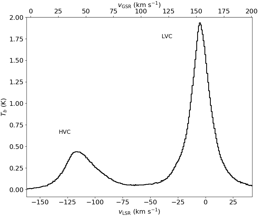
Figure 1: Mean H I  spectrum of the EN dataset from DHIGLS, showing both HVC and LVC peaks well separated by an interval with little emission. Bottom and top axis give velocities in the LSR and GSR, respectively.

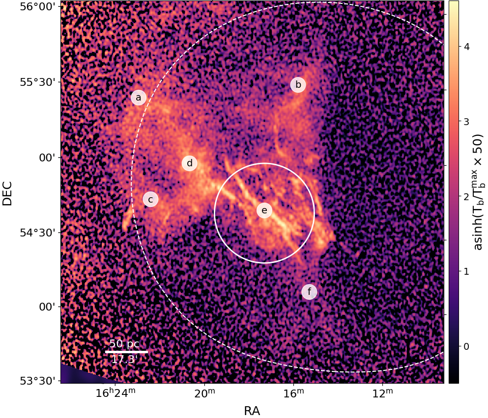
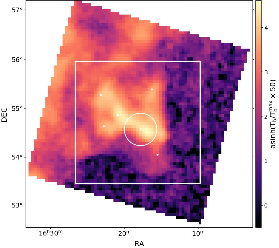
Figure 2: Left: Channel map from the DHIGLS EN data at 1$\farcm$1 resolution for $v_{\rm LSR}=-121$  km s^-1. The area shown is the 6.55 square degrees analysed. Because of the coverage of ST pointings making up the final EN mosaic, the noise increases from a minimum of 0.37 K outward, by a factor two at the open white dashed contour. An asinh non-linear scaling of the brightness has been used to bring this out. White circles labeled (a-f) indicate the positions of the six spectra shown in Fig. 4. The 20′-radius white circle centred on position e corresponds to the beam for profile #26 of Cram & Giovanelli (1976) in which two-component multiphase structure was identified. The physical scale of 50 pc (17$\farcm$3) assumes a distance of 10 kpc. Right: Channel map at lower (10′) resolution and wider coverage from the GHIGLS N1 data. The bright concentration identified as C I B by Giovanelli et al. (1973) is clearly seen at an edge in this broader context. The white box shows the area selected from EN in the left panel.

2 H I  spectral data and decomposition

2.1 Data

The 14.6 square degree EN dataset used in this paper, located at $(\alpha,\,\delta)=(16^{{\mathrm{h}}}$14${}^{{\mathrm{m}}},\,54\degree 49^{\prime})$ or $(l,\,b)=(84\fdg 5,\,44\fdg 3)$ was part of the DHIGLS H I  survey (Blagrave et al., 2017) with the Synthesis Telescope (ST) at the Dominion Radio Astrophysical Observatory. The 256-channel spectrometer, spacing $\Delta v=0.824$  km s^-1and velocity resolution 1.32  km s^-1, was centered at $v_{c}=-60$  km s^-1 relative to the Local Standard of Rest (LSR). The spatial resolution of the ST interferometric data was about 1$\farcm$1. EN is embedded in the N1 field of the GHIGLS H I  survey (Martin et al., 2015) with the Green Bank Telescope (GBT), with spatial resolution about $9\farcm 4$. The DHIGLS EN product has the full range of spatial frequencies, obtained by a rigorous combination of the ST interferometric and GBT single dish data (see Sect. 5 in Blagrave et al., 2017). The pixel size is 18″.

The mean H I  spectrum of the EN dataset is shown in Fig. 1. A velocity range of at least $\Delta v\sim$ 20  km s^-1 with little emission cleanly separates the emission of HVC gas associated with complex C and a low velocity component (LVC) associated with the Milky-Way disk. This important gap coupled with a relatively high fraction of HVC emission limit the confusion between different Galactic environments and, along with the dynamic structure already seen in the N1 data, is what motivated the deep observations with the ST (Blagrave et al., 2017). The top axis of the figure gives the velocity with respect to the Galactic Standard of Rest (GSR):

$$v_{\rm GSR}=v_{\rm LSR}+220\sin(l)\cos(b)\,,$$ (1)

the radial component of the velocity relative to the Sun in a reference frame in which the Galaxy rotates, i.e., removing the effect of the rotation of the LSR about the Galactic Center. This is often thought to be more directly relevant to assessing the kinematics of the HVC gas (Woerden et al., 2004). For a tiny patch like covered by the EN data, the conversion is a simple translation but in the wide-angle context of an entire complex (Sect. 6) it is of more interest.

Figure 2 presents channel maps of HVC emission for $v_{\rm LSR}=-121$  km s^-1, at which the bright concentration C I B was first identified by Giovanelli et al. (1973). On the left is the 6.55 square degree field from the EN data that we analysed and on the right is a corresponding map from the N1 data with the GBT. Both the extent of the bright concentration and the finer spatial structure now available are clearly seen.

As we shall see in much more detail below, most of the diffuse emission is in the upper left triangle of the map; the lower right is relatively void except for a prominent protrusion (“finger”) extending from the main body of emission. The boundary between these triangular areas corresponds to the local “edge” of the much larger complex C and is oriented at position angle about 120° or $-60\degree$. The wider scale context of the concentration C I B is discussed in Sect. 6 and can be seen in Figures 26, 27, and 31 (top right).

The physical scale of 50 pc shown is 17$\farcm$3 at an assumed distance of 10 kpc at this position in complex C. The range of spatial scales accessible (4 pc $\lesssim l\lesssim$ 300 pc) makes C I B a unique laboratory for probing the multi-scale and multiphase properties of neutral gas in HVCs.

2.2 Gaussian decomposition

2.2.1 Model and optimization

We performed multiphase separations of EN and N1 spectra of C I B using the publicly available code ROHSA, a multi-Gaussian decomposition algorithm originally developed for just such analyses. As described by Marchal et al. (2019, hereafter M19), ROHSA is based on a regularized nonlinear least-squares criterion that takes into account the spatial coherence of the emission across a field at coordinates $\bm{r}$ and the multiphase nature of the gas.

The model $\tilde{T}_{b}\big{(}v_{z},\bm{\theta}(\bm{r})\big{)}$ used to fit the measured brightness temperature $T_{b}(v_{z},\bm{r})$ at radial velocity $v_{z}$ and coordinates $\bm{r}$ is

$$\tilde{T}_{b}\big{(}v_{z},\bm{\theta}(\bm{r})\big{)}=\sum_{n=1}^{N}G\big{(}v_{z},\bm{\theta}_{n}(\bm{r})\big{)}\,,$$ (2)

where each of the $N$ Gaussians

$$G\big{(}v_{z},\bm{\theta}_{n}(\bm{r})\big{)}=\bm{a}_{n}(\bm{r})\exp\left(-\frac{\big{(}v_{z}-\bm{\mu}_{n}(\bm{r})\big{)}^{2}}{2\bm{\sigma}_{n}(\bm{r})^{2}}\right)$$ (3)

is parametrized by three 2D spatial fields across $\bm{r}$: $\bm{\theta}_{n}(\bm{r})=\big{(}\bm{a}_{n}(\bm{r}),\,\bm{\mu}_{n}(\bm{r}),\,\bm{\sigma}_{n}(\bm{r})\big{)}$, with amplitude $\bm{a}_{n}\geq\bm{0}$, mean velocity $\bm{\mu}_{n}$, and standard deviation $\bm{\sigma}_{n}$.

The initialization of each Gaussian is accomplished in ROHSA by a multi-resolution procedure from coarse to fine grid (see Sect. 2.4.3 in M19, ). The parameters $\hat{\bm{\theta}}$ are optimized by minimizing a cost function that goes beyond the standard $\chi^{2}$. As described in M19, to penalize variations at the smallest spatial frequencies, the cost function includes Laplacian filtering of each of the three parameter maps $\big{(}\bm{a}_{n},\,\bm{\mu}_{n},\,\bm{\sigma}_{n}\big{)}$, with cost controlled by three hyper-parameters. A fourth penalty term, for minimizing the variance of $\bm{\sigma}_{n}$ across the whole field, is added to enable the multiphase separation. As examined and recommended in M19, the magnitudes of these four hyper-parameters, $\lambda_{\bm{a}},\,\lambda_{\bm{\mu}},\,\lambda_{\bm{\sigma}}$, and $\lambda^{\prime}_{\bm{\sigma}}$, are chosen empirically so that the solution converges toward a noise-dominated residual and a signal that is encoded with a minimum number of Gaussian components.

2.2.2 Decomposition of EN data from DHIGLS

We decomposed the spectra for EN from DHIGLS for the area shown in Fig. 2 (left) and HVC spectral range ($-162.21\leq v_{\rm LSR}$ [ km s^-1] $\leq-60.82$) using $\lambda_{\bm{a}}=1000$, $\lambda_{\bm{\mu}}=100$, $\lambda_{\bm{\sigma}}=1000$, and $\lambda^{\prime}_{\bm{\sigma}}=10$. Because of the relative simplicity of the HVC spectra, as opposed to complex LVC emission from the Milky-Way disk, only a small number of Gaussians, $N=6$, is needed and only four of the six encode emission associated with the HVC; the other two deal with noise at the extreme of the spectral range toward intermediate velocities.

The simple model fits the data well. A map of the reduced chi-squared $\chi^{2}_{r}$ of the decomposition shows no structure, only random fluctuations. Figure 3 shows the one-dimensional probability distribution function (PDF) of $\chi^{2}_{r}$, which peaks near the expected value of 1 denoted by the vertical line.

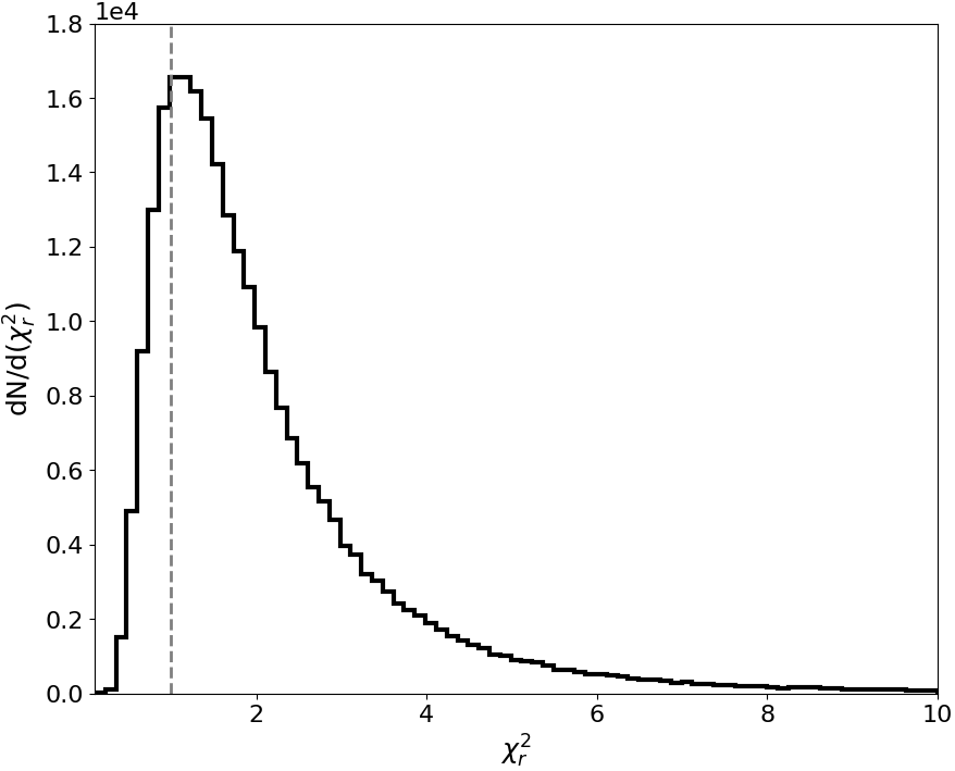
Figure 3: Probability distribution function of the reduced chi-square $\chi^{2}_{r}$ obtained with ROHSA on EN. Vertical line indicates $\chi^{2}_{r}=1$.

Across the field, the spectra are quite varied. Figure 4 illustrates the different decompositions obtained for six lines of sight marked in Fig. 2. Some spectra, particularly in the lower row, contain narrow Gaussian components, indicating the presence of colder gas. Each of these spectra also has emission spread broadly over many channels. This can be fit by broader components, indicating warmer gas, similar to that in the pioneering work of Giovanelli et al. (1973) and Cram & Giovanelli (1976).

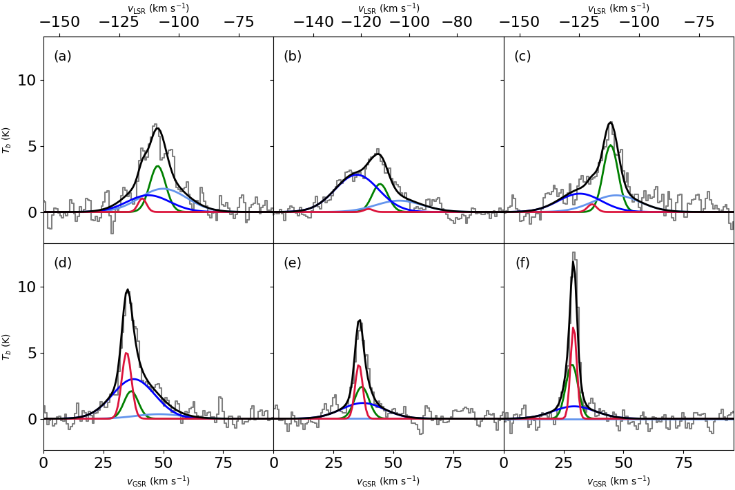
Figure 4: Example Gaussian decomposition by ROHSA for six lines of sight toward C I B, those annotated (a–f) in Fig. 2 (left). The original signal is shown in gray and total signal encoded by ROHSA in black. The four individual Gaussians are color coded: $G_{1}$ (light blue), $G_{2}$ (blue), $G_{3}$ (green), and $G_{4}$ (red).

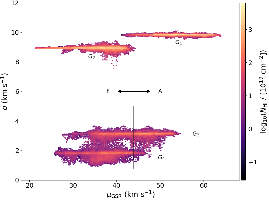
Figure 5: Two-dimensional probability distribution function $\sigma-\mu$

weighted by the column density of each Gaussian along each line of sight. For the two lower clusters $G_{3}$ and $G_{4}$, vertical black line shows the velocity split between region A ($v_{\rm GSR}\geq 44$ km s^-1) and region F.

Table 1: Mean kinematic properties (in  km s^-1) of Gaussians modeling DHIGLS/EN and GHIGLS/N1 data toward C I B

	Component	$G_{1}$	$G_{2}$	$G_{3}$	$G_{4}$
		WNMA	WNMF	LNM	CNM
Field
	$\langle\bm{\sigma}_{n}\rangle$	9.8	8.9	3.1	1.8
EN	$\langle\bm{\mu}_{n}^{\rm{GSR}}\rangle$	55	34.4	44.5	36.8
	$\langle\bm{\mu}_{n}^{\rm{LSR}}\rangle$	$-103.8$	$-124.6$	$-114.8$	$-121.3$
	$\langle\bm{\sigma}_{n}\rangle$	9.6	9.4	7.2	2.6
N1	$\langle\bm{\mu}_{n}^{\rm{GSR}}\rangle$	57.8	25.5	41.1	33.6

It is clear from the original spectra that mean velocities ($\mu$) and dispersions ($\sigma$) of the fitted components vary with position. Figure 5 summarizes the outcome in a two-dimensional PDF of $\sigma-\mu$ weighted by the column density of each Gaussian along each line of sight. In the regularized decomposition obtained with ROHSA, these properties are clustered, each cluster corresponding to one of the four Gaussian components. In particular, the separation vertically into clusters of broader and narrow components results from the hyper-parameter $\lambda^{\prime}_{\bm{\sigma}}$ (M19). Table 1 summarizes the spatially-averaged mean dispersion $\langle\bm{\sigma}_{n}(\bm{r})\rangle$ of each component $n$ and also the mean velocity $\langle\bm{\mu}_{n}(\bm{r})\rangle$, both GSR and LSR.

Clusters $G_{1}$ and $G_{2}$ have similarly large velocity dispersions (separated by only about 1  km s^-1), but cover two distinct velocity ranges and are statistically uncorrelated in their spatial distributions (see Sect. 3.3). Hereafter, these components for two physically distinct regions in this field will be called more memorably WNM_A and WNM_F, respectively, adopting the standard abbreviation WNM for a Warm Neutral Medium “phase”, with subscripts A (“Arc”) and F (“Filaments”) motivated by their different morphologies as described in Sect. 2.4.

This motivated us to identify the unstable (lukewarm) and cold phases, LNM_(A,F) and CNM_(A,F), that are associated with these two regions. To accomplish this within this simple decomposition, the G₃ and G₄ clusters each needs to be divided with respect to velocity $\bm{\mu}_{n}(\bm{r})$. The location of this split was determined by examining the spatial distribution of the emission encoded in the Gaussians, looking for spatial correlations with WNM_A and WNM_F. The resulting split adopted is at $v_{\rm GSR}=44$ km s^-1, marked by the black vertical line in Fig. 5. Not surprisingly, this is close to the velocity extremes where the G₁ and G₂ clusters (WNM_A and WNM_F) separate. Hereafter, gas in clusters G₃ and G₄ with $v_{\rm GSR}\geq 44$ km s^-1 (to the right in the figure) will be called LNM_A and CNM_A, respectively, with the complementary gas being LNM_F and CNM_F.

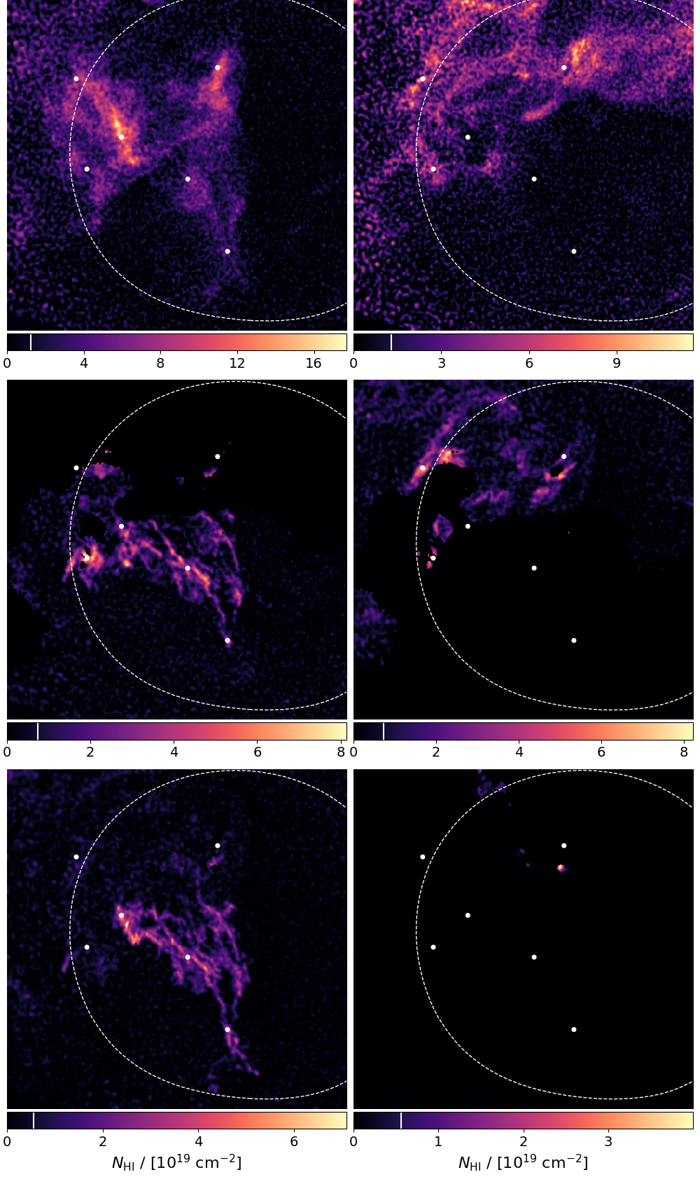
Figure 6: Column density maps of the three HVC phase components identified in two regions of C I B from EN data. (left): WNM_F (top), LNM_F (middle), and CNM_F (bottom); (right): WNM_A (top), LNM_A (middle), and CNM_A (bottom). Note that color bars have different scales. Coordinates (not shown here) are the same as in Fig. 2 (left). The white dots indicate the positions for the six spectra shown in Fig. 4. The white dashed contours indicate where the noise has increased by a factor two relative to the central minimum. The white marks on color bars indicate the column density sensitivity limits (3$\sigma$) within the white dashed contours (see Table 2), showing that the features seen with this color representation are well detected (see also Fig. 29 for another representation).

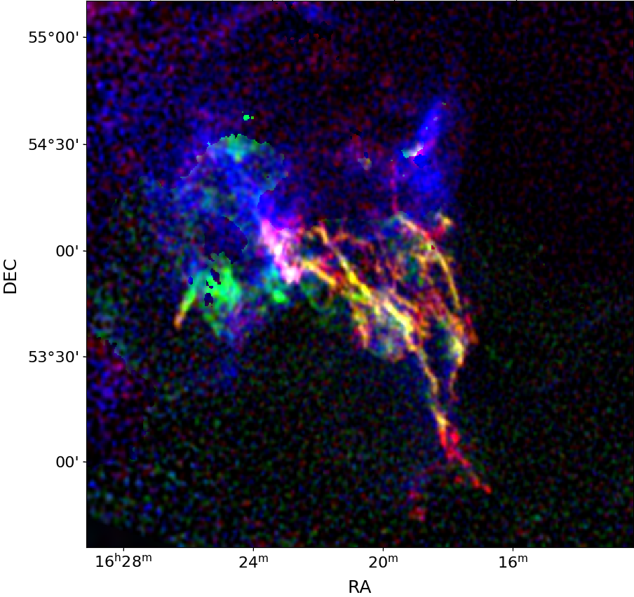
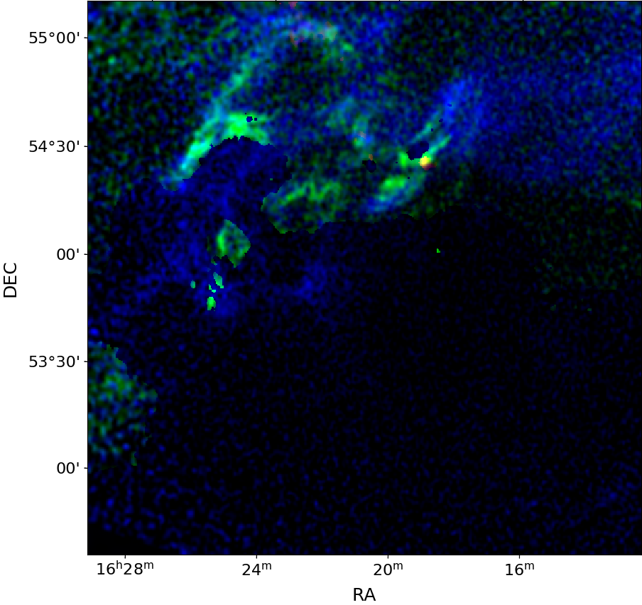
Figure 7: Left: Three-phase view of region F in C I B (EN) from column density maps of WNM_F (blue), LNM_F (green), and CNM_F (red). Maps were scaled with relative weightings of 1, 2, 3 for WNM_F, LNM_F and CNM_F, respectively, to highlight the interrelationship, rather than simply their relative column densities. Right: Same for region A.

2.3 Sensitivity limits

Noise in the spectral data varies over the field, though only by a factor two within the white dashed contour in Fig. 2. In this low-noise central area, the average noise ($3\sigma$) is 1.53 K. Based on this, the corresponding column density sensitivity limit for each phase of regions F and A was evaluated from

$$N_{{\mathrm{H}}\,\mathrm{I}}^{\rm lim}\simeq 0.414\,\sqrt{\langle\sigma(\bm{r})\rangle}\times 10^{19}\,\rm{cm}^{-2}\,,$$ (4)

where $\langle\sigma(\bm{r})\rangle$ is the average dispersion ( km s^-1) of the relevant Gaussians from Table 1. Values are tabulated in Table 2. These are marked on the color bars in Figs. 6 and 29 and can be seen to be reasonable estimates.

Table 2: Column density sensitivity limits (3$\sigma$) by phase (in 10¹⁹ cm^-2)

	WNMF	LNMF	CNMF	WNMA	LNMA	CNMA
$N_{{\mathrm{H}}\,\mathrm{I}}$lim	1.24	0.73	0.56	1.30	0.73	0.56

2.3.1 The impact of spatial resolution

To evaluate the impact of spatial resolution, we performed a decomposition of N1 HVC spectra from the GHIGLS survey in the same velocity range as for the EN data, as detailed in Appendix A. Again ROHSA converges toward four components and a phase separation is still detectable. As seen in Table 1, the mean kinematic properties of Gaussians are fairly similar. The most notable difference is the larger velocity dispersion of $G_{3}$ at the lower spatial resolution of the N1 data (9$\farcm$4 compared to 1$\farcm$1), which would be classified as warm gas. This foreshadows the finding in Sect. 3 that emission in narrow lines (by LNM and CNM gas) has more significant fluctuations on small spatial scales and so is more affected by beam smearing (mixing physically distinct structures inside one beam leads to an unresolved crowding along the velocity axis if their respective velocities are not exactly aligned). In the following, only the higher resolution results are used to analyze the physical properties of the gas toward the concentration C I B.

2.4 Multiphase and multi-scale structure

Figure 6 shows HVC column density maps of the six phases modeled in C I B. Column density detection limits (3$\sigma$, see Table 2) are shown by white marks on the color bars. In region F (right panels), WNM_F, LNM_F, and CNM_F are clearly associated spatially, underlying the split of the $\sigma-\mu$ clusters, especially, LNM ($G_{3}$), in Fig. 5. By contrast, region A shows a dearth of cold gas and emission only in the upper left triangle of the field with a continuous “arc” parallel to the edge in the total column density maps described in Sect. 2.1, Fig. 2.

The finger protruding beyond the edge is traced by WNM_F, LNM_F, and CNM_F and includes very striking elongated filaments along the structure. The close relationship of these filaments to each phase is brought out in Fig. 7 (left), which displays the phases simultaneously, $N_{{\mathrm{H}}\,\mathrm{I}}$ maps of CNM_F, LNM_F, and WNM_F being represented by RGB, respectively). Correlations between phases within each environment and between regions will be quantified statistically in Sect. 3.3.

The other characteristic feature of each $N_{{\mathrm{H}}\,\mathrm{I}}$ map in Fig. 6 is the multi-scale structure. In both regions F and A, lukewarm filaments are visible, often within warmer envelopes. Environment F is furthermore populated with smaller cold filaments within warmer envelopes. Building in this, we focus our analysis on the correlated phases WNM_F, LNM_F, and CNM_F from region F, which are suggestive of an ongoing phase transition where all three phases are present simultaneously. The dearth of cold gas in region A will be discussed in Sect. 6.2.

3 Power spectrum analysis of $N_{{\mathrm{H}}\,\mathrm{I}}$ maps from environment F

To investigate the multi-scale properties, here focusing on region F, we make use of three statistical tools: the power spectrum, the cross power spectrum, and the cross correlation coefficients. For completeness, the results tabulated in Table 3 for region F have their equivalent for region A in Table 4.

3.1 Power spectrum

All spatial (angular) power spectra $P(k)$ presented here are obtained following the methodology described in Martin et al. (2015) and Blagrave et al. (2017). Each power spectrum $P(k)$ is the azimuthal average of the modulus of the Fourier transform of the corresponding field, and is modelled as

$$P(k)=B(k)\times P_{0}k^{\gamma}+N(k)\,,$$ (5)

where, $P_{0}$ is the amplitude of the power spectrum, $\gamma$ is the scaling exponent, $B(k)$ describes the cutoff of the spectrum at high $k$ due to the beam of the instrument, assumed to be a 2D Gaussian of FWHM = 1$\farcm$1, and $N(k)$ is the noise estimated by taking the power spectrum of empty channel maps of the PPV cube. The finite images were apodized using a cosine function to minimize systematic edge effects from the implementation of the Fourier transform.

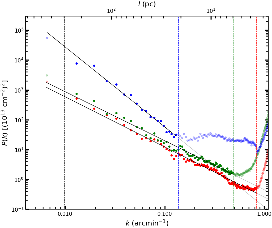
Figure 8: Spatial power spectra and models of the column density maps of WNM_F (blue), LNM_F (green), and CNM_F (red). Corrected (de-convolved) power spectra $P(k)$/$B(k)$ are shown with colored dots. Solid lines show the respective model fits between the vertical dashed lines, chosen to select $k$ ranges avoiding noise or systematics (high- and low-$k$ limits, respectively). Exponents are in Table 3 on the diagonal.

Table 3: Power spectrum analysis of the multiphase region F

	WNMF	LNMF	CNMF
Exponent
WNMF	-2.68$\pm$0.10	-2.51$\pm$0.18	-2.87$\pm$0.37
LNMF		-1.64$\pm$0.03	-2.00$\pm$0.03
CNMF			-1.68$\pm$0.02
Correlation
WNMF	1	0.27$\pm$0.14	0.38$\pm$0.14
LNMF		1	0.53$\pm$0.09
CNMF			1

Table 4: Power spectrum analysis of the multiphase region A

	WNMA	LNMA	CNMA
Exponent
WNMA	-2.37$\pm$0.10	-2.91$\pm$0.50	-2.28$\pm$0.42
LNMA		-1.67$\pm$0.04	-2.16$\pm$0.11
CNMA			-0.53$\pm$0.03
Correlation
WNMA	1	0.32$\pm$0.15	0.10$\pm$0.12
LNMA		1	0.10$\pm$0.12
CNMA			1

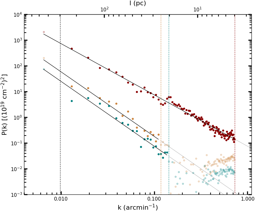
Figure 9: Cross power spectra and models of WNM${}_{\rm F}\times$LNM_F (teal), WNM${}_{\rm F}\times$CNM_F (peru), and LNM${}_{\rm F}\times$CNM_F (dark-red). Corrected cross power spectra $P^{i,j}(k)$/$B(k)$ are shown with colored dots. Solid lines show the respective model fits between the vertical dashed lines. Exponents are in Table 3, off the diagonal.

Figure 8 shows the beam-corrected (de-convolved) spatial power spectra of WNM_F, LNM_F, and CNM_F. LNM_F and CNM_F are well described by power laws in the spatial range 4 pc $\lesssim l\lesssim$ 300 pc. At low spatial frequencies ($k\lesssim$ 0.15), the power spectrum of WNM_F follows a steeper power law. However, at higher $k$, on scales $l\lesssim$ 20 pc, the power spectrum flattens, just as it does for the total $N_{{\mathrm{H}}\,\mathrm{I}}$ of the HVC toward C I B presented by Blagrave et al. (2017, figure 22) using the EN data. This is caused by noise. Unlike CNM_F and LNM_F, the WNM covers parts of the field where the intrinsic noise of the observation is the highest, notably visible in the upper left of WNM_F and WNM_F in Fig 6, outside the white dashed contour that indicates where the noise has increased by a factor two relative to the central minimum. Furthermore, compared to CNM_F and LNM_F, the WNM Gaussian components WNM_F and WNM_F span significantly more channels (i.e., have large velocity dispersions, see Fig. 4), so that again the warm phase is more sensitive to noise (Eq. 4).

Therefore, different spatial ranges are used to fit the power spectrum exponents, as denoted by the vertical dashed lines on the right. These exponents are reported on the diagonal of Table 3. The exponents for LNM_F and CNM_F are significantly less negative (the spectra are flatter) than for WNM_F, quantifying that the unstable and cold phases have relatively more structure on small scales. A similar trend is observed in Table 4 for region A.

3.2 Cross power spectrum

The cross power spectrum $P^{i,j}$(k) is the azimuthal average of the Fourier transform of image $i$ times the conjugate of the Fourier transform of $j$. It is also modeled using Eq. 5. Figure 9 shows the beam corrected spatial cross power spectra of WNM${}_{\rm F}\times$LNM_F, WNM${}_{\rm F}\times$CNM_F, and LNM${}_{\rm F}\times$CNM_F. The cross power spectrum LNM${}_{\rm F}\times$CNM_F is well constrained due to the broad spatial coverage 4 pc $\lesssim l\lesssim$ 300 pc available. On the other hand, WNM${}_{\rm F}\times$LNM_F and WNM${}_{\rm F}\times$CNM_F are dominated by noise on scales $l\lesssim$ 20 pc. Exponents from the model fits are reported in Table 3 in the off-diagonal elements. The cross power spectrum of LNM${}_{\rm F}\times$CNM_F is significantly flatter than WNM${}_{\rm F}\times$CNM_F and WNM${}_{\rm F}\times$LNM_F, considering the uncertainties.

The cross power amplitude of LNM${}_{\rm F}\times$CNM_F is much higher than for the other two cross powers, but similar to the amplitudes for these cooler components in Fig. 8, revealing a strong correlation between these two maps. The exponent for LNM${}_{\rm F}\times$CNM_F is somewhat steeper than for the power spectrum of CNM_F, indicating a relative de-correlation at the smallest scales.

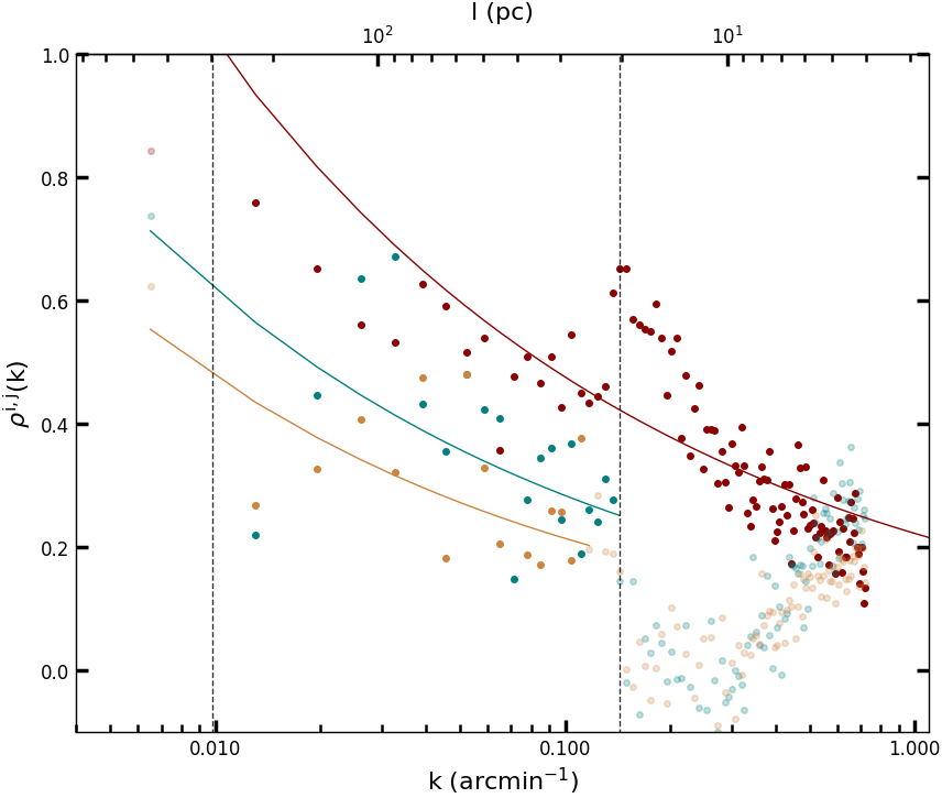
Figure 10: Cross correlation coefficients $\rho^{i,j}(k)$ of LNM${}_{\rm F}\times$CNM_F (dark-red), WNM${}_{\rm F}\times$CNM_F (peru), and WNM${}_{\rm F}\times$LNM_F (teal). Calculated coefficients are shown with colored dots. Solid lines are based on the spectral fits shown in Figs. 8 and 9. Vertical dashed lines shows high- and low-$k$ limits within which the mean and standard deviation of the correlation coefficient for each pair are computed (see Table 3).

3.3 Cross correlation coefficients

For further statistical quantification of the interrelationship between phases, we combined the power spectra and the cross power spectra results to obtain the cross correlation coefficients $\rho^{i,j}(k)$ for each pair of column density maps, formally

$$\rho^{i,j}(k)=\frac{P^{i,j}(k)}{\sqrt{P^{i,i}(k)\,P^{j,j}(k)}}\,.$$ (6)

Figure 10 shows the cross correlation coefficients of LNM${}_{\rm F}\times$CNM_F, WNM${}_{\rm F}\times$CNM_F, and WNM${}_{\rm F}\times$LNM_F. Solid lines show the models $\tilde{\rho}^{i,j}(k)$ obtained using the spectral fits shown in Figs. 8 and 9. Note again the de-correlation toward smaller spatial scales.

In addition, for each pair we calculated the mean and standard deviation (not uncertainty) of the cross correlation coefficients in the spatial range $20$ pc $<l<300$ pc. These results are tabulated in Table 3 (bottom section). The correlation of LNM${}_{\rm F}\times$CNM_F is the highest and as seen in Fig. 10 the other two are not negligible. But in region A, only WNM${}_{\rm A}\times$LNM_A has a hint of correlation.

Finally, for WNM${}_{\rm A}\times$WNM_F we find a cross correlation coefficient of $-0.01\pm 0.13$, which confirms that regions A and F are uncorrelated statistically and should be analyzed independently.

4 Properties of structures from segmentation of $N_{{\mathrm{H}}\,\mathrm{I}}$ maps in region F

As can be appreciated from Fig. 6 (left), the surface coverage of the EN data is large enough to explore substructures within each phase of region F of C I B. The largest scale ($\sim 400$ pc) allows us to segment even the warm phase and the smallest scale ($\sim 2$ pc) allows us to quantify the finer structures seen in the colder phase. For completeness, results of a similar analysis for region A are given in Appendix C.

4.1 Hierarchical clustering of $N_{{\mathrm{H}}\,\mathrm{I}}$ maps from region F using dendrograms

To perform the clustering analysis, we made use of the astrodendro python package that follows the changing topology of the isosurfaces as a function of their contour levels (Rosolowsky et al., 2008). Our choice of this specific method was motivated by the potentially multi-scale nature of the observed phase transition, a direct consequence of turbulence. Also, as noted by Goodman et al. (2009), a dendrogram is almost entirely data driven and is weakly sensitive to the chosen user-parameters.

A detailed description is provided in Appendix B where visualizations of the extracted structures are shown in the left panels of Fig. 29 (see right panels for region A). We obtained $N_{c}=21,$ 60, and 73 structures for WNM_F, LNM_F, and CNM_F, respectively.

In separate subsections below, we have evaluated a number of properties of the structures – physical, thermodynamic, and turbulent – for each phase and for the total ensemble. The values have a considerable range, so that their PDFs are best displayed logarithmically. Although the PDFs are not precisely log-normal, they are well summarized by the mean and standard deviation of the log of the parameter. The value of the parameter corresponding to this mean is reported in Table 5, along with the standard deviation (hereafter “spread”, e.g., 2 for a 0.3 dex standard deviation) in parenthesis.

4.1.1 Evaluation of uncertainties

To evaluate the uncertainties of physical properties derived from dendrograms, we have repeated the segmentation on $N_{{\mathrm{H}}\,\mathrm{I}}$ maps using two series of decompositions obtained with ROHSA. For the first series, composed of 50 runs, in the spectral data for each line of sight we injected Gaussian random noise with the same dispersion as the noise in the original data. The hyper-parameters were kept the same. For the second series, composed of 80 runs, we kept the original data cube (i.e., each run has just the original noise) but randomly perturbed the four ROHSA hyper-parameters in a $\pm 10$% interval around the original values. From the catalogs obtained by segmentation for each run, properties of the structures – physical, thermodynamic, and turbulent – were computed.

The new structures extracted were cross-matched with structures in the original catalogs using their spatial coordinates. The uncertainties of the properties of a structure were estimated by calculating the standard deviation over the cross-matched members for each series. Finally, for each property the contributions from the two series were summed in quadrature to yield the total uncertainty (the contribution from the first series was generally slightly higher than from the second).

These uncertainties were then taken into account in producing the PDFs presented below. In each PDF, the bin size (logarithmically constant) was chosen so that it was larger than the relative uncertainty of the quantity being analyzed in each bin.

4.2 Physical properties

Table 5: Properties of structures in region F

	Symbol	WNMF	LNMF	CNMF	TotalF	Units
	$N_{c}$	21	60	73	154
Physical
Size	$L$	28 (1.6)	7.3 (1.4)	6.4 (1.4)	8.2 (1.8)	pc
Aspect ratio	$r$	2.0 (1.4)	2.1 (1.5)	2.1 (1.5)	2.1 (1.5)
Mass	$M_{{\mathrm{H}}\,\mathrm{I}}$	296 (3.4)	18 (2.3)	12 (1.9)	22 (3.8)	M⊙
Average number of H atoms per unit volume	$n$	0.41 (1.9)	1.4 (1.8)	1.3 (1.9)	2.1 (2.1)	cm-3
Thermodynamic
Doppler velocity dispersion	$\sigma_{T_{b}}$	8.9 (1.0)	3.0 (1.1)	1.6 (1.1)	2.6 (1.8)	km s-1
Turbulent velocity dispersion	$\sigma_{v_{z}}$	0.79 (2.4)	0.94 (1.6)	0.74 (1.8)	0.82 (1.8)	km s-1
Thermal velocity dispersion	$\sigma_{\rm th}$	8.8 (1.0)	2.7 (1.1)	1.3 (1.4)	2.3 (2.0)	km s-1
Kinetic temperature	$T_{k}$	9.5 (1.0)	0.90 (1.2)	0.20 (2.1)	0.62 (4.0)	103 K
Sound speed	$C_{s}$	9.6 (1.0)	3.0 (1.1)	1.4 (1.4)	2.5 (2.0)	km s-1
Thermal crossing time	$t_{\rm cross}^{\rm th}$	2.8 (1.6)	2.4 (1.5)	4.5 (1.8)	3.3 (1.8)	Myr
Turbulent crossing time	$t_{\rm cross}^{v_{z}}$	34 (2.1)	7.6 (1.5)	8.5 (1.7)	9.8 (2.1)	Myr
Thermal pressure	$P_{\rm th}/k_{B}$	3.8 (1.9)	1.2 (1.8)	0.25 (2.8)	0.70 (3.7)	103 K cm-3
Turbulent pressure	$P_{\rm v_{z}}/k_{B}$	0.1 (7.6)	0.5 (2.3)	0.3 (3.1)	0.3 (3.7)	103 K cm-3
Total pressure	$P_{\rm tot}/k_{B}$	4.5 (1.9)	2.0 (1.6)	0.7 (1.8)	1.4 (2.5)	103 K cm-3
Turbulent cascade
Turbulent sonic Mach number	$\mathcal{M}_{s}$	0.14 (2.4)	0.55 (1.7)	0.86 (2.2)	0.56 (2.5)
Mean free path	$\lambda$	0.80 (1.9)	0.24 (1.8)	0.25 (1.9)	0.29 (2.1)	10-3 pc
Kinematic molecular viscosity	$\nu$	1.0 (1.9)	0.09 (1.8)	0.05 (2.0)	0.09 (3.3)	1021 cm2 s-1
Knudsen number	$K_{n}$	2.9 (1.8)	3.2 (1.5)	4.0 (1.6)	3.5 (1.6)	10-5
Reynolds number	$Re$	0.62 (3.9)	2.1 (1.9)	2.7 (2.4)	2.0 (2.7)	104
Dissipation scale	$\eta$	4.0 (2.5)	0.42 (1.6)	0.30 (1.9)	0.49(2.9)	10-2 pc
Dissipation time	$t_{\eta}$	4.9 (3.9)	0.59 (1.9)	0.61 (2.3)	0.80 (3.1)	10-1 Myr
Convective time	$t_{L}$	38 (3.9)	8.5 (1.9)	10 (2.3)	11.3 (3.1)	Myr
Traversal time	$\tau_{L}$	39 (2.1)	8.6 (1.5)	10.1 (1.6)	11.4 (2.0)	Myr
Energy transfer rate	$\epsilon$	0.22 (11)	1.4 (3.7)	0.6 (4.1)	0.7 (5.3)	10-5 L⊙ M${}_{\odot}^{-1}$

Note. — Values correspond to the mean and spread from the logarithmic PDF.

The sky coordinates of a structure in a particular frame (taken to be the International Celestial Reference System for the terminology here) are the mean positions of all pixels, weighted by column density:

$$(\bar{x},\bar{y})=\sum_{\bm{r}}(x(\bm{r}),y(\bm{r}))\,N_{{\mathrm{H}}\,\mathrm{I}}(\bm{r})\,/\,\sum_{\bm{r}}N_{{\mathrm{H}}\,\mathrm{I}}(\bm{r})\,,$$ (7)

where $x$ and $y$ denote the Right Ascension and Declination.

The geometry of each structure is modeled by an on-sky ellipse. Following Hennebelle & Audit (2007) and Miville-Deschênes et al. (2017), the inertia matrix of the projected emission is

$$I=\left[\begin{array}[]{ll}\sigma_{x}^{2}&\sigma_{xy}^{2}\\ \sigma_{xy}^{2}&\sigma_{y}^{2}\end{array}\right]\,,$$ (8)

where the matrix coefficients are

$$\sigma_{xy}^{2}=\sum_{\bm{r}}\left(x(\bm{r})-\bar{x}\right)\left(y(\bm{r})-\bar{y}\right)N_{{\mathrm{H}}\,\mathrm{I}}(\bm{r})\,/\,\sum_{\bm{r}}N_{{\mathrm{H}}\,\mathrm{I}}(\bm{r})\,.$$ (9)

4.2.1 Size

Using the eigenvalues $\lambda_{\rm min}$ and $\lambda_{\rm maj}$ of $I$ and the pixel area $S_{A}=(D\delta)^{2}$ (the scaling with distance $D$ can be tracked), the lengths of the semi-major and semi-minor axes are $L_{{\rm min,\,maj}}=\sqrt{8\ln(2)\,S_{A}\,\lambda_{{\rm min,\,maj}}}$. Making the assumption that the depth along the line of sight is more likely to be $L_{\rm min}$, the volume of the ellipsoid is $V=(4\pi/3)\,L_{\rm min}^{2}L_{\rm maj}$. Finally, our size estimate is simply $L=V^{1/3}$.

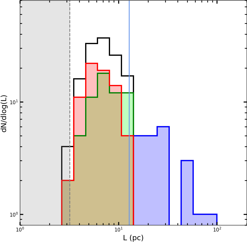
Figure 11: Probability distribution function of the typical size $L$ of structures extracted from WNM_F (blue), LNM_F (green), and CNM_F (red). The total shown in black. The gray dashed line shows physical size of 1$\farcm$1 beam at 10 kpc. The blue vertical line shows physical size of 4$\farcm$4 beam (i.e., the convolved WNM_F map used for the clustering) at the same distance.

Figure 11 shows the PDFs of the size, with color coding for each phase. The PDF for all phases combined is also shown in black (note the logarithmic scale vertically). Sizes range from $\sim$ 3 pc (the spatial resolution of the maps for LNM_F and CNM_F, see vertical gray dashed line) up to $\sim$ 100 pc.

Inspection of Fig. 11 suggests that the PDF of $L$ for CNM_F and LNM_F might be impacted by the resolution, 1$\farcm$1 or 3.2 pc at the assumed distance. Perhaps smaller structures would be identified with observations of higher resolution and higher signal to noise. In none of the statistics, here and below, have we applied any correction for this potential bias. Similarly, because the segmentation for WNM_F was carried out on maps convolved to 4$\farcm$4 (a factor of four in resolution, see vertical blue line for the corresponding physical size), that phase too is potentially impacted. Even so, there is some evidence that the typical size of structures decreases from the warmer to the cooler phases, as expected from the thermal condensation.

4.2.2 Aspect ratio

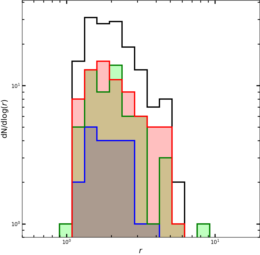
Figure 12: Probability distribution function of the aspect ratio $r$ of structures extracted from WNM_F (blue), LNM_F (green), and CNM_F (red). The total is shown in black.

Figure 12 shows the PDFs of the aspect ratio $r=L_{\rm maj}/L_{\rm min}$. In each phase, $r$ is generally higher than 1.5 and can reach values up to 6 in CNM_F and LNM_F. The shape of the distributions looks similar among phases and the mean of all distributions is close to 2 (see Table 5), showing that elongated structures are seen not just in the cold phase but rather are a multiphase property.

4.2.3 Orientation

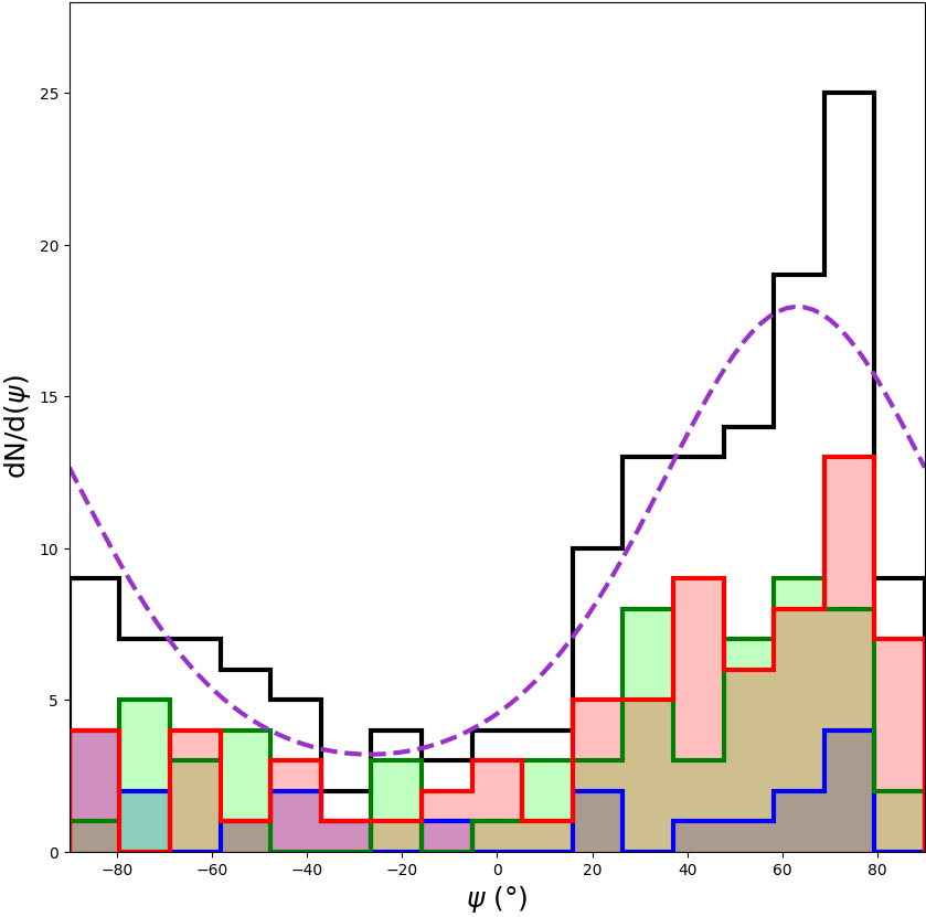
Figure 13: Probability distribution function of the position angle $\psi$ of structures extracted from WNM_F (blue), LNM_F (green), and CNM_F (red). The total is shown in black. The purple dashed line shows the MLE fit of the Von Mises distribution to the (unbinned) orientations of all structures.

The position angle $\psi$ of each structure is

$$\psi=tan^{-1}\left(\frac{v_{2}}{v_{1}}\right)\,,$$ (10)

where $(v_{1},\,v_{2})$ is the eigenvector corresponding to $\lambda_{m\rm ax}$.

Figure 13 shows the PDF of $\psi$ for each phase and the whole sample. CNM_F and LNM_F clearly show a distribution dominated by positive position angles; the evidence for WNM_F is less pronounced. Maximum Likelihood Estimates (MLE) of the location (orientation) and dispersion of a Von Mises distribution fit to the orientations of all of the structures are $+63\degree$ and $31\degree$, respectively. The purple dashed line shows the model.

In region A, we find an orientation of $-43\degree$ and a dispersion of $38\degree$ (see Fig. 30 in Appendix C). That the mean orientations of structures in regions F and A are roughly orthogonal can be appreciated visually from Figs. 6 and 7.

4.2.4 Mass

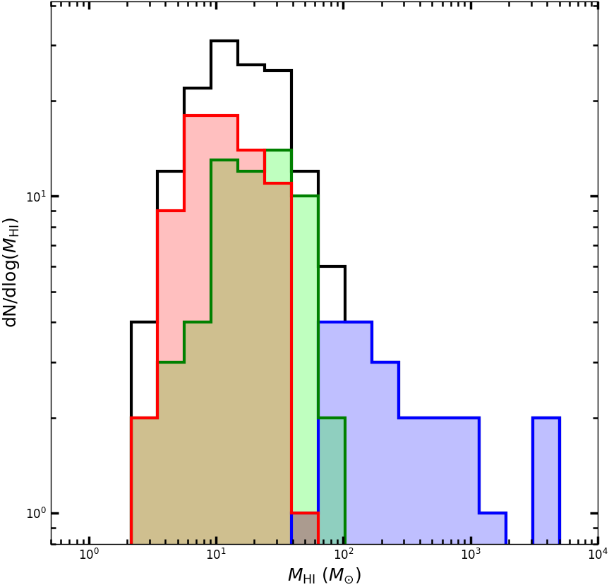
Figure 14: Probability distribution function of the mass $M_{{\mathrm{H}}\,\mathrm{I}}$ of structures extracted from WNM_F (blue), LNM_F (green), and CNM_F (red). The total is shown in black.

The mass of each structure derived from the column density is

$$M_{{\mathrm{H}}\,\mathrm{I}}=S_{A}\,\mu_{m}\,m_{\rm H}\,\sum_{p}N_{{\mathrm{H}}\,\mathrm{I}}^{p}\,.$$ (11)

Here $m_{\rm H}$ is the mass of the hydrogen atom and $\mu_{m}=1.4$ accounts for the atomic Galactic composition, so that $M_{{\mathrm{H}}\,\mathrm{I}}$ is actually the total mass of the neutral gas.

Figure 14 shows the PDFs of $M_{{\mathrm{H}}\,\mathrm{I}}$. Masses increase systematically from CNM_F to LNM_F and WNM_F, with values ranging from $\sim$ 2 $M_{\odot}$ in the cold phase up to $\sim$ 3000 $M_{\odot}$ in the warm phase. Note that CNM structures would reach even lower masses if they were segmented more finely at higher spatial resolution.

The total masses of CNM_F, LNM_F, and WNM_F are $(1,1.5,{\rm and\,}15)\times 10^{3}$ $M_{\odot}$, respectively. The corresponding mass fractions within region F are 0.06, 0.08, and 0.86. Finally, for perspective, the total mass of the neutral gas of these structures, $18\times 10^{3}$ $M_{\odot}$, is just 0.3% of the total atomic mass of complex C (Thom et al., 2008).

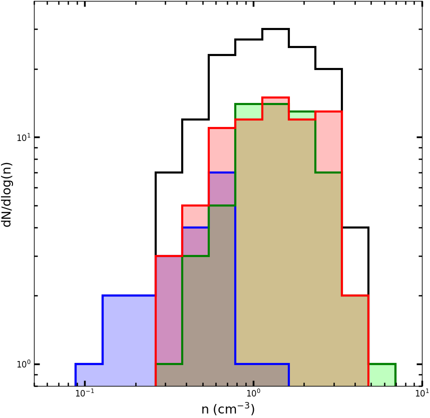
Figure 15: Probability distribution function of the average number density of H atoms $n$ of structures extracted from WNM_F (blue), LNM_F (green), and CNM_F (red). The total is shown in black.

4.2.5 Average number density of H atoms

For each structure, the average number of H atoms per unit volume is

$$n=\frac{1}{\mu_{m}m_{\rm H}}\frac{M_{{\mathrm{H}}\,\mathrm{I}}}{V}\,,$$ (12)

(or equivalently the total column density $N_{{\mathrm{H}}\,\mathrm{I}}$ times $S_{A}$ divided by $(4\pi/3)\,L_{\rm min}^{2}L_{\rm maj}$) which scales as $D^{-1}$. Figure 15 shows the PDFs of $n$. From the condensation mode of thermal instability we expect to observe an increase of the $n$ from the warm to the cold phase. There is some evidence for this, and it is possible that $n$ for CNM_F is underestimated because of the finite resolution.

4.3 Thermodynamic properties

4.3.1 Separation of thermal and non-thermal motions

The observed Doppler dispersions $\sigma_{T_{b}}$ of the structures (Table 5) measure the total velocity dispersion of gas along the line of sight. This is often modeled as a quadratic sum of a thermal component and a non-thermal component

$$\sigma_{T_{b}}=\sqrt{\sigma_{\rm th}^{2}+\sigma_{v_{z}}^{2}}\,.$$ (13)

Separation of the two components is not possible using data for a single line of sight, but can be done statistically for an ensemble. According to studies by Ossenkopf et al. (2006, and references therein), for a turbulent medium the statistics of the 3D velocity field can be recovered from its 2D projection if density fluctuations are small compared to the mean density of the fluid ($\sigma_{\rho/\rho_{0}}\lesssim 0.5$).

To verify that sufficiently small density contrast is the case here, the methodology proposed by Brunt et al. (2010) and applied to 21 cm line emission data in Marchal & Miville-Deschênes (2021) was used to calculate, for each structure, the density contrast of its three-dimensional (3D) density field $\sigma_{\rho/\rho_{0}}$ from the column density contrast of its projection along the line-of-sight $\sigma_{N/N_{0}}$. Brunt et al. (2010), assuming that the statistical properties of $\rho$ are isotropic and using Parseval’s Theorem, have shown that the ratio of these contrasts is

$$R =\left(\frac{\sigma_{N/N_{0}}}{\sigma_{\rho/\rho_{0}}}\right)^{2}$$ (14)

$$=\frac{\left(\sum\limits_{k_{x}=-L_{\rm min}/2+1}^{L_{\rm min}/2}\sum\limits_{k_{y}=-L_{\rm maj}/2+1}^{L_{\rm maj}/2}P^{3D}_{\rho}(k)\right)-P^{3D}_{\rho}(0)}{\left(\sum\limits_{k_{x}=-L_{\rm min}/2+1}^{L_{\rm min}/2}\sum\limits_{k_{y}=-L_{\rm maj}/2+1}^{L_{\rm maj}/2}\sum\limits_{k_{z}=-L_{\rm min}/2+1}^{L_{\rm min}/2}P^{3D}_{\rho}(k)\right)-P^{3D}_{\rho}(0)}\,,$$ (15)

where $P^{3D}_{\rho}(k)$ is the azimuthally-averaged power spectrum of $\rho$.

For a structure of size $L_{\rm min}\times L_{\rm maj}$, two parameters control the ratio $R$: the slope of $P^{3D}_{\rho}(k)$ and the depth of the structure. For this model we consider $P^{3D}_{\rho}(k)\propto k^{-11/3}$, representative of a sub/trans-sonic turbulence. The depth over which velocity fluctuations are averaged is assumed to be $L_{\rm min}$, so that $R$ depends on the aspect ratio $r$ of each structure. For the whole sample, we find a mean value $\sigma_{\rho/\rho_{0}}\sim 0.2$ and a standard deviation of 0.1. This result is not sensitive to a variation of $\pm 1/3$ for the slope of $P^{3D}_{\rho}(k)$.

Having verified that density fluctuations are sufficiently small, using the same formalism (i.e., the same coefficient $R$ for each structure), we can infer the non-thermal velocity dispersion $\sigma_{v_{z}}$ of the three-dimensional (3D) velocity field from the observed dispersion of its projection along the line of sight, $\sigma_{\left<v_{z}\right>_{z}}$. We find a similar velocity dispersion $\sigma_{v_{z}}$ across phases (Table 5), with a value about 0.8  km s^-1 overall. This is a significant part of the Doppler dispersion only for the CNM, as reflected in the thermal velocity dispersions $\sigma_{\rm th}$ recorded, derived using Eq. 13. Formally, nothing prevents the inferred value of $\sigma_{\rm th}$ from being less than the channel spacing of the observations. However, this occurs for only 9 out of the 73 structures in CNM_F and for these there is considerable uncertainty.

Properties derived below that are dependent on these separated velocity dispersions are less directly data-driven than the physical quantities in Sect. 4.2. Nevertheless, tabulating these provides a global view of the properties of the fluid constituting the concentration C I B, which is useful for interpreting our results in the context of condensation via thermal instability.

4.3.2 Velocity dispersions and related properties

The inferred kinetic temperature is $T_{k}=\sigma_{\rm th}^{2}\,m_{\rm H}/k_{B}$, where $k_{B}$ the Boltzmann constant and as used here $\sigma_{\rm th}$ describes the motions of H atoms. The adiabatic sound speed is $C_{s}=\sqrt{\gamma k_{B}T_{k}/\mu_{m}m_{\rm H}}\equiv\sqrt{\gamma/\mu_{m}}\,\sigma_{\rm th}$, with the adiabatic index $\gamma=5/3$ for atomic gas. In combinations with the size of the structure, the thermal crossing time is $t_{\rm cross}^{\rm th}=L/C_{s}$ and the turbulent crossing time is $t_{\rm cross}^{v_{z}}=L/\sigma_{v_{z}}$.

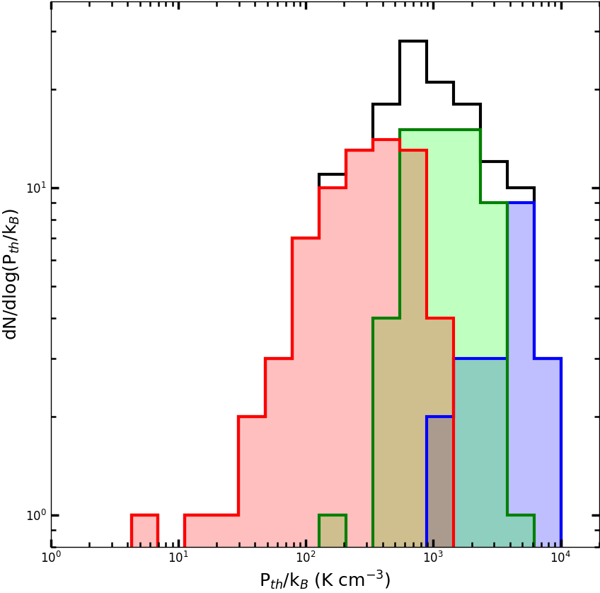
Figure 16: Probability distribution function of the thermal pressure $P_{\rm th}/k_{B}$ of structures extracted from WNM_F (blue), LNM_F (green), and CNM_F (red). The total is shown in black.

4.3.3 Thermal pressure

Given the kinetic temperature and the average number density of H I of a structure, the thermal pressure is

$$P_{\rm th}/k_{B}=\mu_{P}\,n\,T_{k}\equiv\mu_{P}\,n\,\sigma_{\rm th}^{2}m_{\rm H}/k_{B}\,,$$ (16)

with $\mu_{P}=1.1$ accounting for He. Figure 16 shows the PDFs of $P_{\rm th}/k_{B}$ for the phases. There is an apparent decrease of mean thermal pressure from WNM_F to LNM_F and CNM_F (see also Table 5). As mentioned in Sect. 4.2.5, because of finite resolution the average number of H atoms per unit volume of CNM structures might be higher than that above, which would increase the thermal pressure. A secondary compensating effect might be less beam smearing, possibly leading to a lower estimate of the thermal broadening and therefore a lower thermal pressure.

4.4 Turbulent and total pressure

The turbulent pressure can be calculated using the deduced turbulent velocity dispersion:

$$P_{\rm t}/k_{B}=3\,\mu_{P}\,n\,\sigma_{\rm v_{z}}^{2}m_{\rm H}/k_{B}\,.$$ (17)

where the factor 3 account for the dimensionality of $\sigma_{\rm v_{z}}$ (from 1D to 3D). As expected from the typical relative sizes of $\sigma_{\rm v_{z}}$ and $\sigma_{\rm th}$ (Table 6), this pressure is of most interest in the CNM phase. The total pressure is just $P_{\rm tot}/k_{B}=(P_{\rm t}+P_{\rm th})/k_{B}$. Table 6 gives the mean and spread of each quantity calculated for the ensemble.

4.5 Properties of the turbulent cascade

Turbulent fluids are commonly characterized by properties like the Mach number. These can be derived from the velocity dispersions in combinations with the size $L$ and average number of H atoms per unit volume $n$, and so again can be considered as different recastings not as directly data-driven. They are nevertheless useful in connecting to the literature and understanding numerical simulations. Values of such properties are given in Table 5 for structures in different phases. These are motivated and discussed briefly here.

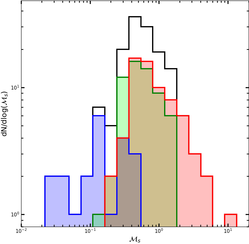
Figure 17: Left: Probability distribution function of the sonic Mach number $\mathcal{M}_{s}$ of structures extracted from WNM_F (blue), LNM_F (green), and CNM_F (red). The total is shown in black.

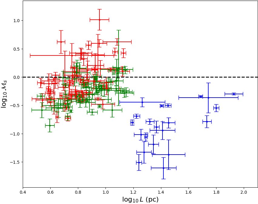
Figure 18: Scatter plot of $\log_{10}\mathcal{M}_{s}$ vs $\log_{10}L$. Values for structures from CNM_F, LNM_F, and WNM_F are shown in red, green, and blue, respectively. The black dashed line indicates $\mathcal{M}_{s}=1$.

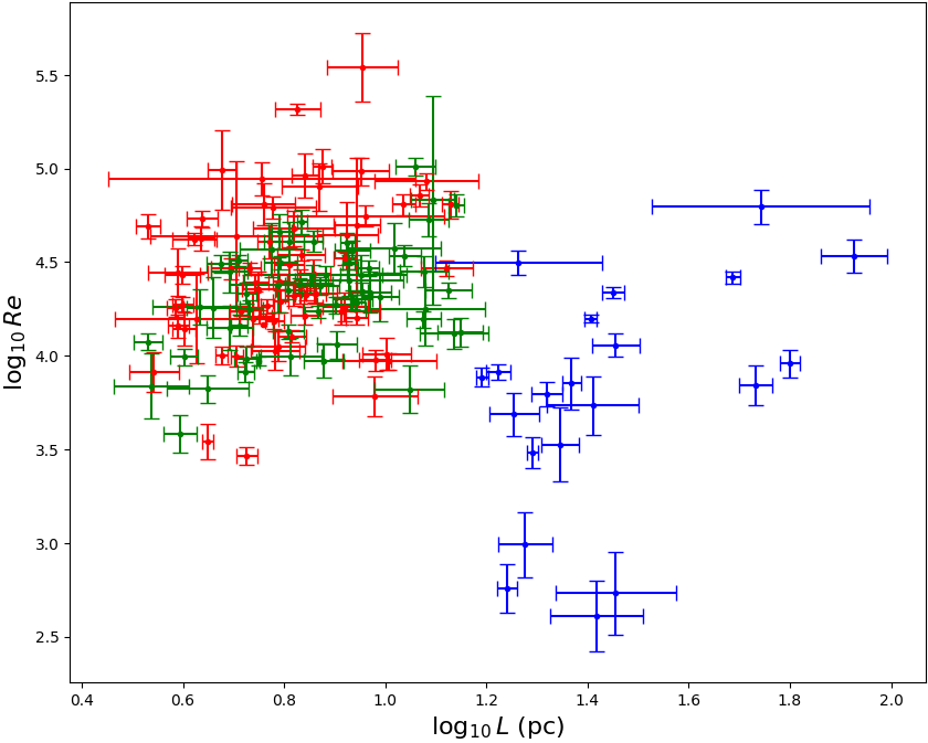
Figure 19: Scatter plot of $\log_{10}Re$ vs $\log_{10}L$. Values for structures from CNM_F, LNM_F, and WNM_F are shown in red, green, and blue, respectively. The black dashed line indicates $\mathcal{M}_{s}=1$.

The turbulent sonic Mach number $\mathcal{M}_{s}$ of a structure is

$$\mathcal{M}_{s}=\frac{\sqrt{3}\,\sigma_{v_{z}}}{C_{s}}\,.$$ (18)

Figure 17 shows the PDFs of $\mathcal{M}_{s}$. Because $\sigma_{v_{z}}$ is fairly constant, $\mathcal{M}_{s}$ increases from the warm phase to the cold phase, from a sub-sonic regime ($0.14\,(2.4)$) to a trans-sonic regime ($0.75\,(2.1)$). This implies an inverse trend of $\mathcal{M}_{s}$ with size, as shown in as Fig. 18.

For properties below involving a mean free path, $\lambda$, we assume $\lambda=1/(n\,\sigma$ with $\sigma=1\times$10^-15 cm² for the hydrogen collision cross-section (Lequeux, 2012). One such property is the kinematic viscosity

$$\nu=\frac{1}{3}\lambda\,v_{\rm th}\,,$$ (19)

where the arithmetic mean speed $v_{\rm th}=\sqrt{8/\pi\gamma}C_{s}\equiv\sqrt{8/\pi\mu}\,\sigma_{\rm th}$.

Another such property is the Knudsen number $Kn=\lambda$/$L$. For an isothermal gas, as assumed here for each individual structure, the ratio of $\mathcal{M}_{s}$ to the Knudsen number is linked directly to the Reynolds number

$$Re=\sqrt{\frac{\pi}{2}}\frac{\mathcal{M}_{s}}{Kn}\,,$$ (20)

which quantifies the relative influence of advection and diffusion in a turbulent fluid. Unlike $\mathcal{M}_{s}$, $Re$ is proportional to $n$, through the inverse dependence on $\lambda$. The net dependence on size is shown in the scatter plot of $Re$ and $L$ in Fig. 19. We observe the same trend as for $\mathcal{M}_{s}$, i.e., $Re$ increases from large warm structures to small cold structures. The typical values of $Re$ are of interest too. If initial perturbations applied to a flow are not too small, turbulence appears at $Re\sim 2000$ (Reynolds, 1883). It therefore seems likely that the turbulence in gas toward C I B is well developed for CNM_F, LNM_F, and even WNM_F, except for four structures with $Re<1000$ (Fig. 19).

Other combinations give characteristic size and time scales for structures. The dissipation scale $\eta$, on which the smallest eddies dissipate the turbulent energy into heat through viscosity, is

$$\eta=LRe^{-3/4}\,,$$ (21)

and the dissipation time scale $t_{\eta}$ is

$$t_{\eta}=\frac{\eta^{2}}{\nu}\,.$$ (22)

Note that $\eta$ and $t_{\eta}$ are also called the Kolmogorov length and time scales. The convective time, also called the large eddy turnover time, is

$$t_{L}=t_{\eta}Re^{1/2}\,.$$ (23)

The traversal time $\tau_{L}$ needed for an eddy of size $L$ to traverse the inertial range, in which viscous effects are essentially negligible, down to the Kolmogorov length scale $\eta$ is related to $Re$ through the relation

$$\tau_{L}=\frac{t_{L}}{1-Re^{-1/2}}\,.$$ (24)

For high $Re$, i.e., fully developed turbulence, $\tau_{L}\sim t_{L}$. Finally, combining the dissipation scale and the dissipation time, the energy transfer rate $\epsilon$ is

$$\epsilon=\frac{\eta^{2}}{t_{\eta}^{3}}\,.$$ (25)

4.6 Scaling laws between properties of extracted structures

4.6.1 Mass and density – size relations

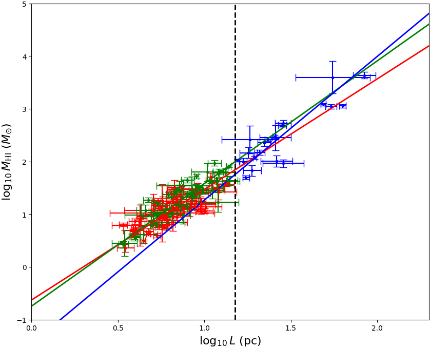
Figure 20: Scatter plot of $\log_{10}M_{{\mathrm{H}}\,\mathrm{I}}$ vs $\log_{10}L$. Values for structures from CNM_F, LNM_F, and WNM_F are shown in red, green, and blue, respectively. Pearson correlation coefficients are 0.90, 0.81, and 0.76, respectively. Solid lines show power law fits using the bisector estimator. Black dashed line marks our estimate of the cooling length scale, at which the warm gas undergoes a phase transition.

A scatter plot of H I  mass (proportional to total column density: Eq. 11) and size is shown in Fig. 20, color coded by phase. Note the logarithmic scales, such that the slope in this diagram is the power-law exponent of the mass-size relation. Using a bisector estimator of the slopes, the exponents are $2.7\pm 0.2$, $2.2\pm 0.2$, and $2.0\pm 0.1$ for WNM_F, LNM_F, and CNM_F, respectively.

Recognizing the uncertainties, we find that the exponent for WNM_F is higher than those of LNM_F and CNM_F. This trend is consistent with the ranking of the exponents found in Sect. 3 for the power spectra of the column density maps (Fig. 8 and Table 3), that for WNM_F being steeper.

By definition, $M\propto n\,L^{3}$. The deviations of the above exponents from 3 show that the average number of H atoms per unit volume $n$ is not constant even within a single phase. Instead, $n$ varies inversely with $L$, with exponents $-0.3\pm 0.2$, $-0.8\pm 0.2$, and $-1.0\pm 0.1$ for WNM_F, LNM_F, and CNM_F, respectively. The increase of $n$ from large to small scales is more pronounced in the unstable and cold phases compared to the warm phase, a result of the thermal condensation.

Finally, we have made an empirical estimate of the typical cooling length scale at which the warm gas is non-linearly unstable (Audit & Hennebelle, 2005). This should be larger than most LNM_F and CNM_F structures and so from Fig. 11 $\lambda_{\rm cool}\sim 15$ pc, as marked by the vertical black dashed line in Fig. 20. This spatial scale is five times higher that the spatial resolution of the observation (also the size of the smallest cold structures) and this estimate is only weakly sensitive to the user parameters of the dendrograms. Note also that this result is driven by the largest structures extracted in LNM_F (i.e., 14.1 pc) as opposed to the smallest structures found in WNM_F. Therefore, it is not affected by the limited spatial resolution of the WNM_F map from the convolution applied to suppress noise (see Appendix B).

4.6.2 Turbulent velocity dispersion – size relation

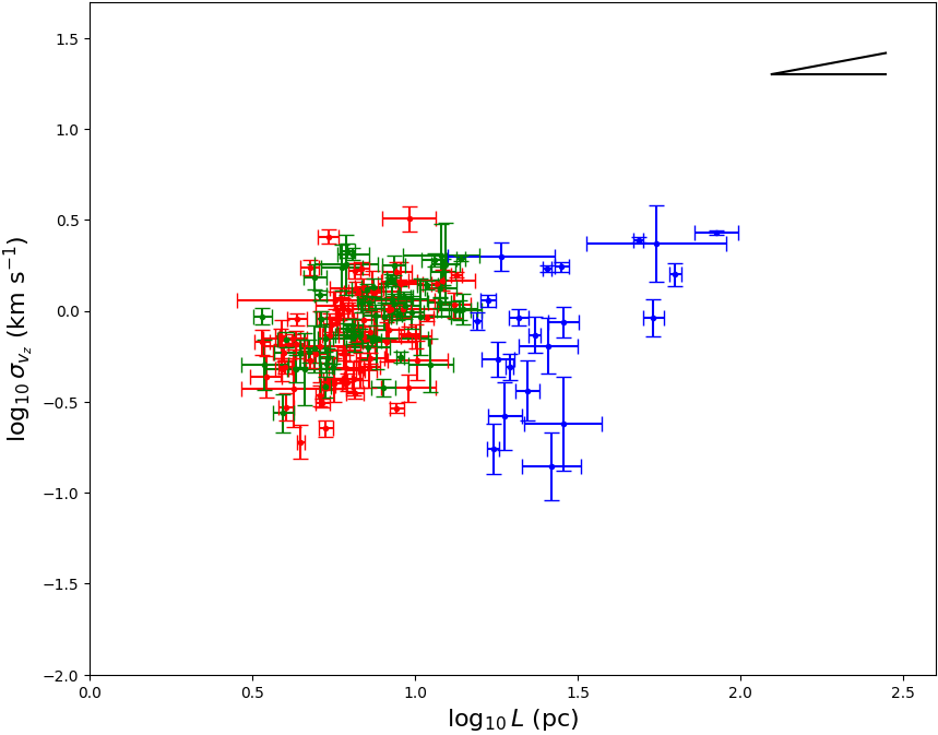
Figure 21: Scatter plot of $\log_{10}\sigma_{v_{z}}$ vs $\log_{10}L$. Values for structures from CNM_F, LNM_F, and WNM_F are shown in red, green, and blue, respectively. The Pearson correlation coefficient is 0.27 for the ensemble. The theoretical slope 1/3 of sub/trans-sonic turbulence is illustrated in the upper right corner.

Figure 21 shows the $\sigma_{v_{z}}-L$ relation, color coded by phase. The two variables are positively correlated, with Pearson correlation coefficient is 0.27. Although the Pearson coefficient is significantly positive, its value is too low for a reliable determination of the power law exponent. Given the Mach numbers obtained in Sect. 4.5, one might expect to see the scaling law of sub/trans-sonic compressible turbulence (Kim & Ryu, 2005), close to Kolmogorov’s prediction of incompressible turbulence $\sigma_{v_{z}}\propto L^{1/3}$ (Kolmogorov, 1941). This is illustrated in the top right corner of Fig. 21.

4.6.3 Kinematic viscosity and energy transfer rate – size relations

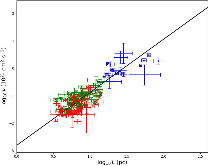
Figure 22: Scatter plot of $\log_{10}\nu$ vs $\log_{10}L$. Values for structures from CNM_F, LNM_F, and WNM_F are shown in red, green, and blue, respectively. The Pearson correlation coefficient is 0.83 for the ensemble and solid black line shows a power law fit.

Figure 22 shows the kinematic viscosity as a function of scale. The Pearson correlation coefficient is 0.83 for the ensemble and a power-law fit using the bisector estimator gives exponent $1.9\pm 0.1$. Noting that $\nu\propto T_{k}^{1/2}n^{-1}$ from Eq. 19, this pronounced scaling is seen to be a direct consequence of the phase transition, which lowers the kinetic temperature and increases the average number of H atoms per unit volume of the fluid as the scale decreases.

The Pearson correlation coefficient of the energy transfer rate – size scaling law (not plotted) is -0.06, showing that no significant trend is observed.

4.6.4 Insights into the turbulent cascade

In summary, the physical properties of structures extracted from region F across phases reveal the presence of a sub/trans-sonic turbulent energy cascade. The warm component is the least turbulent phase with $Re=0.62\,(3.9)\times 10^{4}$.

When the fluid undergoes a phase transition, condensed gas with higher $n$ and lower $T_{k}$ appears as smaller structures and filaments (see Figs. 6 (left), 7 (left), 11, and 12). This change in the thermodynamic properties of the gas modifies a fundamental property of the turbulence, the kinematic viscosity $\nu$. The scale dependence of $\nu$ (Fig. 22) increases the relative strength of turbulence from large scales to small scales (see Fig. 19 for $Re$ and Figs. 17 and 18 for $\mathcal{M}_{s}$). There is a progression from subsonic to trans-sonic turbulence, reaching a state characterized by $\mathcal{M}_{s}=($0.86 (2.2)$)$ in the coldest phase (Table 5).

Despite this change in the statistical properties of the turbulent cascade, a constant energy transfer rate is observed over scales. This favors a scenario where no energy is injected or dissipated along the energy cascade. In other words, this turbulence appears to be self-similar, even if influenced by a phase transition.

The traversal time $\tau_{L}$ decreases from the warm phase to the cold phase (Table 5). This suggests that velocity fluctuations (and therefore density fluctuations) will last longer in the warm phase than in the cold phase. Note that in each phase the traversal time and turbulent crossing time $t_{\rm cross}^{v_{z}}$ are very similar.

5 Thermal equilibrium and thermal instability

The following discussion relates to the interpretation of thermal properties of the structures in different phases in region F. While it is difficult to demonstrate unequivocally that the colder and denser condensations that are observed have formed simply by a triggered thermal instability, we find multiple pieces of evidence pointing in this direction.

5.1 Thermal equilibrium

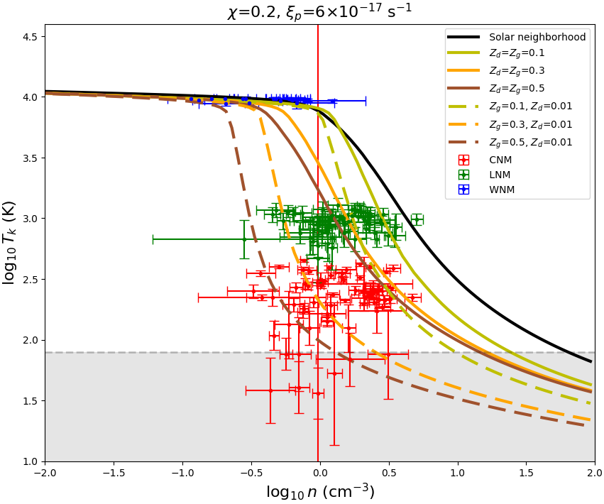
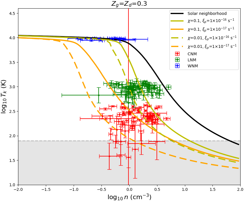
Figure 23: $\log_{10}T_{k}$ – $\log_{10}n$ diagram showing values for structures extracted from WNM_F, LNM_F, and CNM_F, in blue, green, and red, respectively. These data are repeated in left and right panels. The gray dashed line shows the kinetic temperature corresponding to the channel spacing of the observations. Superimposed are theoretical thermal equilibrium curves for a range of model parameters. Left: Colored and dashed lines show curves for varying gas phase metallicity ($Z_{g}$) and dust-to-gas ratio ($Z_{d}$), with fixed FUV interstellar radiation field strength ($\chi=0.2$) and the primary CR ionization rate ($\xi_{p}=6\times 10^{-17}$ s^-1). The black line shows the equilibrium curve for solar neighborhood conditions ($\chi=1$ and $\xi_{p}=2\times 10^{-16}$ s^-1). Right: Colored and dashed lines show curves for varying $\chi$ and $\xi_{p}$, for a fixed gas phase metallicity and dust-to-gas ratio $Z_{g}=Z_{d}=0.3$.

5.1.1 Empirical $T_{k}$ – $n$ diagram and some caveats

Figure 23 shows the $T_{k}$ -$n$ diagram for structures extracted from WNM_F, LNM_F, and CNM_F, color coded by phase. There are nine structures from CNM_F with $T_{k}$ below the horizontal gray dashed line (see Sect. 4.3.1) and these have large uncertainties.

It is instructive to use this figure for comparisons with thermal equilibrium models, but there are some effects that could compromise the comparison in its detail. First, for each phase the dispersion in $T_{k}$ is much smaller than that in $n$. For WNM_F, this is expected because the steep temperature dependence of cooling by collisional excitation of Ly-$\alpha$ constrains the temperature of the warm gas to a narrow range close to $T_{k}\sim 10^{4}$ K. However, for the LNM_F and CNM_F, we would not expect the gas to be so closely isothermal for different structures. The narrowness of the range of $T_{k}$ found arises at least in part from our spectral decomposition using ROHSA, which in enabling phase separation favors a solution with each Gaussian component having a similar Doppler velocity dispersion across the field, as is apparent in Fig. 5. The non-thermal component of the dispersion is fairly uniform, and so this propagates to the derived uniformity in $T_{k}$. Therefore, the ensemble for a given phase, LNM_F or CNM_F, provides a single estimate of the typical temperature for that phase and any temperature variation with density is lost.

Second, the observed $\sigma_{T_{b}}$ for CNM_F, which is quite small, might be biased high by two effects, beam smearing (Sect. 4.2.1) and the finite spectral resolution of the spectrometer. This bias would propagate such that $T_{k}$ might then be lower than we have inferred.

Third, as discussed in Sect. 4.2.1, the limited spatial resolution of the observation is likely to lower the inferred average number of H atoms per unit volume of extracted structures for CNM_F. Allowing for these last two effects, the red dots for structures from CNM_F might tend to be shifted down and/or to the right in Fig. 23.

5.1.2 Modeling the thermal state in C I B

We have calculated the thermal state of the gas using the approximation of a static 1D photodissociation region (PDR) model at the location of C I B in the Galactic halo. This is admittedly oversimplified, but should be a useful benchmark toward deeper understanding. In particular, we calculated the thermal equilibrium curve $\mathcal{L}=0$ using the chemical network presented in Gong et al. (2017), where $\mathcal{L}$ is the net heating and cooling. In the neutral atomic phase of the ISM, heating is dominated by photo-electrons from small dust grains and cooling is dominated by collisional excitation of Ly-$\alpha$ and fine structure lines of OI, CII, and CI. Input parameters of this PDR model are the FUV interstellar radiation field strength $\chi$ (in units of the Draine (1978) field strength, Draine, 1978), the dust abundance $Z_{d}$ and the gas metallicity $Z_{g}$ (each relative to the value in the solar neighborhood), and the primary cosmic ray (CR) ionization rate per H atom, $\xi_{p}$.

To choose plausible values of $\chi$ and $\xi_{p}$, we first evaluated these parameters at the Galactocentric radius of C I B, $R_{\rm C\,I\,B}=11$ kpc, using table 2 in Wolfire et al. (2003). We then applied the scaling with height $z$ above the Galactic plane using equation 4 in Wolfire et al. (1995b), assuming $z=10\,\sin(b_{\rm C\,I\,B})$ kpc. In addition, $\chi$ was multiplied by a factor of 0.6 to lower the midplane intensity to the intensity at the surface of the disk, in order to match the FUV optical depth obtained by Tielens & Hollenbach (1985) (Wolfire et al., 1995b). This approach led to $\chi\sim 0.2$ and $\xi_{p}=6\times 10^{-17}$ s^-1. These values anchor ranges that we have explored. We note that an X-ray radiation field that might assume some importance in the Galactic halo is not included in the model. Its potential effects might be mimicked in part by larger values of these two parameters.

Three gas phase metal abundances, $Z_{g}=(0.1,0.3,0.5)$, were selected ranging over estimated metallicities in complex C (Gibson et al., 2001; Collins et al., 2003, 2007; Tripp et al., 2003). The choice of $Z_{d}$ is more problematic because no dust has been detected in HVCs to date; we explored two possibilities, dust limited by the metallicity, $Z_{d}=Z_{g}$, and a much lower value $Z_{d}=0.01$.

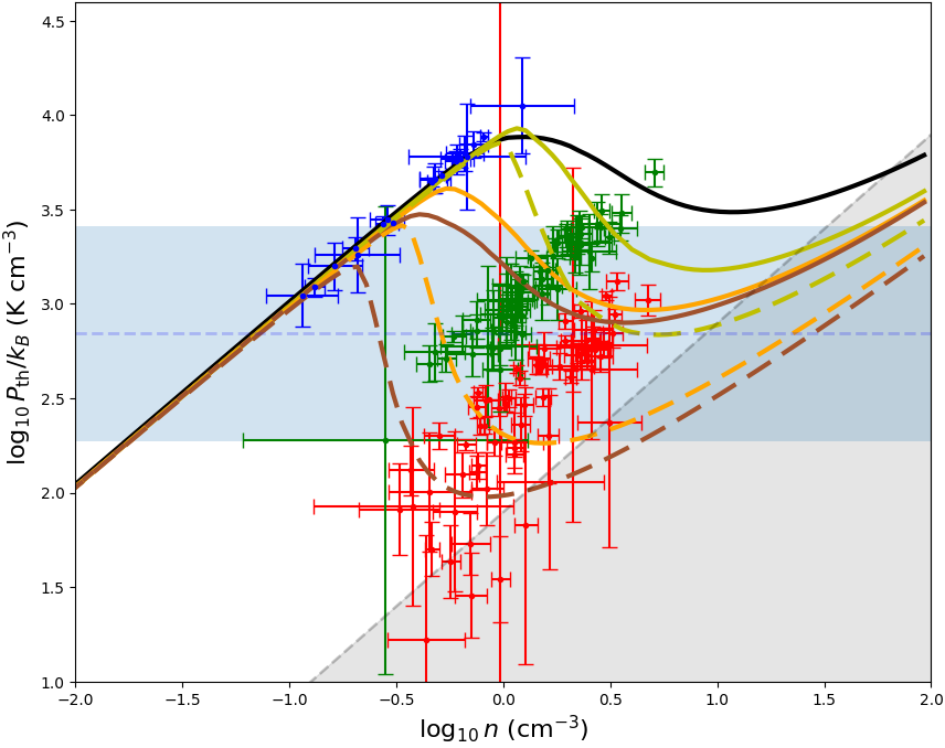
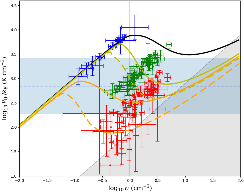
Figure 24: Like Fig. 23 but for a $\log_{10}P_{\rm th}/k_{B}$ – $\log_{10}n$ diagram. The blue horizontal dashed line and surrounding shaded area show the mean and spread of the thermal pressure for the ensemble of structures in region F.

5.1.3 Comparison of models and data

Results of our explorations of parameter space are summarized in the two panels in Fig. 23. Any comparisons made with the properties inferred independently from the data (hereafter, data) are subject to the previous caveats.

In the left panel, colored lines and dashed lines show thermal equilibrium curves for varying metallicity and dust abundance, with fixed $\chi=0.2$ and $\xi_{p}=6\times 10^{-17}$ s^-1. Solid lines are for different pairs of $Z_{g}=Z_{d}=(0.1,0.3,0.5)$. The stability of these curves when $Z_{g}$ and $Z_{d}$ are decreased simultaneously arises because the photoelectric heating by dust is roughly proportional to $Z_{d}$ and the gas cooling is roughly proportional to $Z_{g}$, so that changes in these two processes track each other and the change in $\mathcal{L}$ is small. If the dust abundance $Z_{d}$ is reduced without changing $Z_{g}$, the photo-electric heating is reduced, leading to lower temperatures (dashed curves). In each case, the theoretical thermal equilibrium curve $\mathcal{L}=0$ is unable to reproduce the data in WNM_F, LNM_F, and CNM_F simultaneously. For example, in the case of $Z_{g}=0.3$ and $Z_{d}=0.01$ (dashed orange curve), the theoretical $\mathcal{L}=0$ curve shows rough agreement with the average values in CNM_F but does not extend to the higher density structures seen in the other phases.

In the right panel, solid and dashed lines show thermal equilibrium curves of varying FUV interstellar radiation field strength ($\chi=0.1$ or $\chi=0.01$) and CR ionization rate ($\xi_{p}=10^{-16}$ s^-1 or $\xi_{p}=10^{-17}$ s^-1), for a fixed metallicity and dust abundance ($Z_{g}=Z_{d}=0.3$). Reducing $\chi$ directly reduces the photo-electric heating. Reducing $\xi_{p}$ reduces the electron abundance (ionization fraction of the gas), which then also reduces the efficiency of photo-electric heating. Similar to the left panel, no single theoretical thermal equilibrium curve can reproduce the range of data seen in all three phases. The model with $\chi=0.1$ and $\xi_{p}=10^{-17}$ s^-1 (solid orange curve) passing through the cloud of points for CNM_F, again fails to reproduce the higher densities seen in the other phases.

5.1.4 Deviation from a single thermal equilibrium curve

Although general trends relating to phase separation are present in static models with heating and cooling mechanism in equilibrium, no single thermal equilibrium curve can reproduce the data. There are many failure modes. For example, models that allow a broad range of WNM_F densities predict warmer LNM_F and CNM_F at their inferred densities.

One possible explanation might be local variations in the physical environment ($\chi$ and $\xi_{p}$) or in the gas ($Z_{g}$ and $Z_{d}$). However, given the relatively low gas surface density ($N_{\mathrm{HI}}\gtrsim 2\times 10^{20}~{}\mathrm{cm^{-2}}$, see Fig. 6) and metallicity, significant variations in $\chi$ and $\xi_{p}$ from shielding are not expected, except perhaps in the densest parts of CNM_F that are not well resolved. Local variations of metallicities would require a higher $Z_{g}$ or lower $Z_{d}$ in LNM_F and CNM_F. Plausible local variations of $Z_{g}$ might arise if the H I  observed in C I B is a mixture of the original infalling HVC and the Galactic halo material (Heitsch et al. 2021, in preparation). Local variations of $Z_{d}$ might be produced by mixing with halo material and/or local destruction of dust due to the systematic motions in the encounter.

Alternatively, the gas might just be out of thermal equilibrium. This possibility is implied by the lower thermal pressure in LNM_F and CNM_F (see Table 5) and is supported by the fact that the dynamical timescale (thermal crossing times in Table 5) is comparable to the cooling timescale (see also Sect. 5.2.2). A related caution (or hint) is the widespread presence of the LNM_F phase, which the models suggest is thermally unstable.

5.2 Thermal instability

In the ISM, the formation and steady-state presence of non-gravitational cold condensations has been related to the condensation mode of thermal instability (Field, 1965). To assess the relevance of this physical mechanism to the observed phase transition in EN, we evaluated whether perturbations around the mean thermodynamic state of the gas in C I B would allow the condensation mode of thermal instability to develop and then to grow freely.

5.2.1 Development of the condensation mode

In an idealized non-viscous static fluid in thermal equilibrium, the isobaric criterion for development of the condensation mode of thermal instability can be expressed as

$$\left(\frac{\partial P}{\partial n}\right)_{\mathcal{L}=0}<0$$ (26)

(Field, 1965; Wolfire et al., 1995a). To assess whether this idealized criterion is satisfied in the mean pressure and density range where the phase separation is observed in EN, the properties extracted from WNM_F, LNM_F, and CNM_F are presented in the relevant $P_{\rm th}/k_{B}$ – $n$ phase diagram in Fig. 24, color coded by phase. The mean and spread of the thermal pressure of all structures in C I B are indicated by the light blue line and shaded area. This is lower than in standard models of the solar neighborhood ISM (e.g., Wolfire et al., 1995a, see also the black curves in Fig. 24). The data also reveal the relevant density range to consider.

Superimposed on the two panels are model thermal equilibrium curves corresponding to those presented in Fig. 23. As in the discussion in Sect. 5.1, there is no single model that reproduces the data. However, in the average number of H atoms per unit volume range observed in EN, where a number of the plausibly relevant models do intersect with the mean pressure in LNM_F and CNM_F (green and red points), we can see directly that the curves satisfy Eq. 26. On average, from WNM_F to LNM_F and CNM_F, the pressure drops and the density increases, also satisfying Eq. 26. Thus, depending on the actual local net cooling of the gas in the C I B conditions, pressure perturbations around the average pressure might plausibly trigger the condensation mode of thermal instability, leading to the phase separation observed.

5.2.2 Can the condensation mode grow freely?

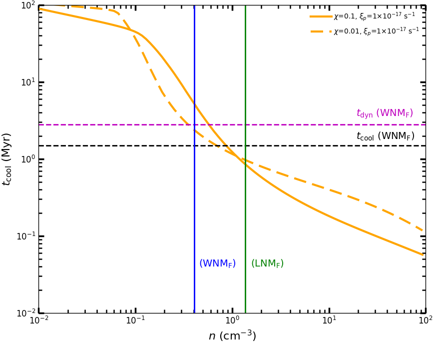
Figure 25: Curves of cooling time versus $n$ for thermal equilibrium models with parameters $\chi=0.2$, $\xi_{p}=6\times 10^{-17}$ s^-1, $Z_{d}=0.01$, $Z_{g}=0.3$ (orange dashed curve), and $\chi=0.01$, $\xi_{p}=1\times 10^{-17}$ s^-1, $Z_{d}=Z_{g}=0.3$ (orange solid curve). The horizontal black dashed line shows the typical cooling time in the WNM_F from Eq. 28. The magenta dashed line shows $t_{\rm dyn}$, the mean thermal crossing time of WNM_F (Table 5). Vertical lines show the mean density of structures from WNM_F and LNM_F, blue and green respectively.

A second criterion, i.e., ensuring that the condensation mode can grow freely, involves dynamical and cooling time scales. When the gas experiences a perturbation (i.e., a compression), condensation is possible if the cooling time of the fluid element is shorter than its dynamical time (Hennebelle & Pérault, 1999):

$$\mathcal{I}=t_{\rm cool}/t_{\rm dyn}<1\,.$$ (27)

The fact that we observe a phase separation implies that $\mathcal{I}<1$ is satisfied. The presence of LNM gas further suggests that the phase transition is ongoing.

The dynamical time, the typical thermal crossing time of the warm phase WNM_F, is about 2.8 Myr (Table 5). Understanding the balance between time scales requires an assessment of $t_{\rm cool}$ in C I B.

First, we inferred $t_{\rm cool}$ from

$$t_{\rm cool}=\lambda_{\rm cool}/C_{s}^{\rm WNM_{1}}\,.$$ (28)

where the typical cooling length $\lambda_{\rm cool}$ was estimated in Sect. 4.6.1 to be about 15 pc. Using $C_{s}^{\rm WNM_{1}}=9.6$  km s^-1, we find $t_{\rm cool}\sim 1.5$ Myr. Compared to the dynamical time, $\mathcal{I}<1$ is satisfied weakly.

Second, we evaluated the theoretical cooling time for the models presented in Sect. 5.1. A selection of the curves is shown in Fig. 25 as a function of $n$. They correspond to the models with parameters $\chi=0.2$, $\xi_{p}=6\times 10^{-17}$ s^-1, $Z_{d}=0.01$, $Z_{g}=0.3$ (orange dashed curve as in Fig. 23 (left), and $\chi=0.01$, $\xi_{p}=1\times 10^{-17}$ s^-1, $Z_{d}=Z_{g}=0.3$ (orange solid curve as in Fig. 23 right). As discussed above, these models do not reproduce the dispersion observed in the $T_{k}-n$ diagram but they provide examples of consistent models approximating the average thermodynamic state of the gas in C I B and establish the plausibility of thermal instability (Fig. 24). For comparison, the horizontal black dashed line shows the typical cooling time from Eq. 28. The magenta dashed line shows the above estimate of $t_{\rm dyn}$ from the mean thermal crossing time of structures from WNM_F, which are larger than $\lambda_{\rm cool}$. Vertical lines show the mean density of structures from WNM_F and LNM_F, in blue and green respectively (see Table 5), bounding the range of typical densities where condensation is observed. In that range, these example models have cooling times that are compatible with the Eq. 28 estimate and also suggestively close enough to $t_{\rm dyn}$ to allow some perturbations to satisfy $\mathcal{I}<1$.

6 Origin of substructure in the large-scale context of complex C

Elongated structures (Fig. 12) are a multi-scale property of the flow in region F. Structures and filaments are very well correlated across phases and scales (Figs. 9 and 10), which indicates that the phase transition is already spatially and anisotropically shaped on large scales. There is no homogeneous warm phase of H I  from which the cooler structures condense.

There is some evidence for the importance of thermal instability in the phase transition (Sect. 5), but thermal equilibrium models are obviously not adequate to describe the complex physical state arising from the interaction of the HVC gas with the Galactic halo. Investigation of the mechanisms that are generated at large scales, lead to the observed thermal condensation, and shape the gas will require numerical simulations.

Simulations in turn need to be set up with appropriate geometries and initial conditions. With observations of just small areas like C I B, this would be challenging, even misleading. For example, the HVC gas in the N1 field has been classified morphologically to be among the substantial sub-population of compact HVCs that show prominent head-tail structure (Brüns et al., 2000). However, the observed CNM here occurs in what in that phenomenology is the “tail”. Of more fundamental importance, this gas is not isolated and so it is instructive to consider the context of its place in complex C.

6.1 Large-scale view from EBHIS

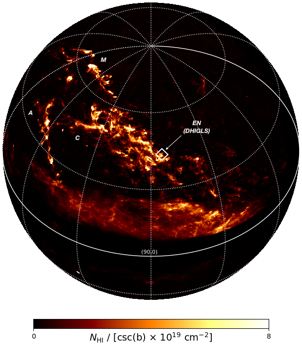
Figure 26: Orthographic projection of $N_{{\mathrm{H}}\,\mathrm{I}}$ of HVC gas selected from EBHIS using $v_{\rm{DEV}}<-80$  km s^-1 ($|v_{\rm{DEV}}|>80$  km s^-1), showing the location of C I B along a projected edge. The white box shows the coverage selected from EN similar to Fig. 2 (right).

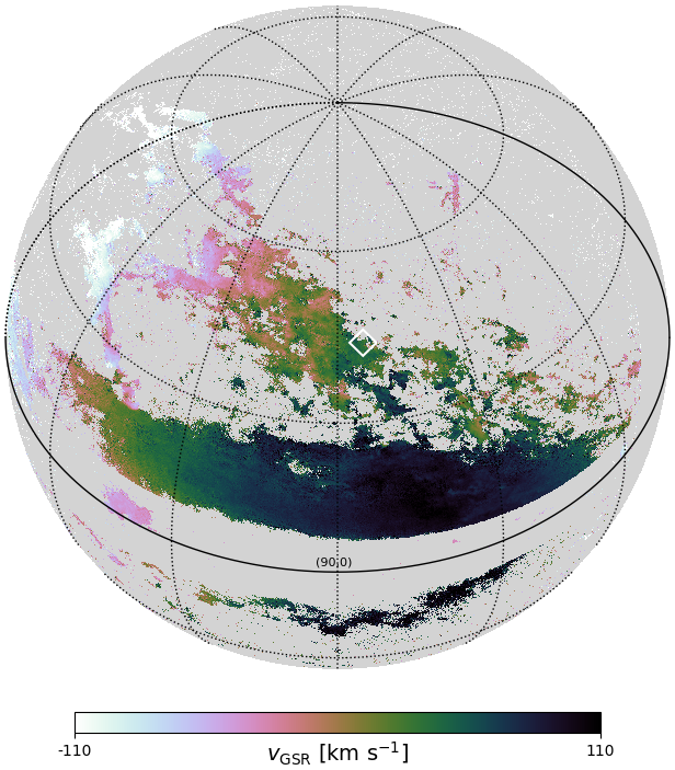
Figure 27: Orthographic projection of the centroid velocity field of the HVC gas in Fig. 26. Note that the velocity is shown in the Galactic Standard of Rest (GSR). The centroid velocity can be calculated even at low $N_{{\mathrm{H}}\,\mathrm{I}}$ but the gray background corresponds to a mask with $N_{{\mathrm{H}}\,\mathrm{I}}<0.5\times 10^{19}$ cm^-2. The white box shows the coverage selected from EN.

This is enabled by the wide sky coverage of the EBHIS data (Kerp et al., 2011; Winkel et al., 2016). Surveyed with the Effelsberg 100-meter radio telescope, EBHIS has a spatial resolution comparable to GHIGLS (10$\farcm$8 and 9$\farcm$4 beams, respectively). To select only the HVC emission, we used the deviation velocity $v_{{\rm DEV}}$ (Appendix D), which measures the difference between the observed $v_{\mathrm{LSR}}$ and the predicted velocities of gas throughout a model H I  disk. In complex C and its neighborhood, $v_{\mathrm{LSR}}$ and $v_{\rm{DEV}}$ are negative. Selecting $v_{\rm{DEV}}<-80$  km s^-1 ($|v_{\rm{DEV}}|>80$  km s^-1) isolates the HVC from the IVC emission (particularly the extended “Intermediate Velocity Arch” (IV Arch, Kuntz & Danly, 1996) that would be included at smaller deviations.

Figure 26 shows a map of the column density $N_{{\mathrm{H}}\,\mathrm{I}}$ of the selected HVC emission, in an orthographic projection centred on $(l,\,b)=(90\degree,\,45\degree)$, close to C I B at $(l,\,b)=(84\fdg 5,\,44\fdg 3)$ indicated by the white arrow. The column density is dominated by complex C and its neighbors, complexes A and M. Most of the emission from the Galactic plane has been removed by the $v_{{\rm DEV}}$ cut, but some emission from the Milky-Way extra-planar gas is still visible at $\lvert b\rvert\leq 30\degree$ (Marasco & Fraternali, 2011). The relative prominence of this non-HVC emission is suppressed by imaging $N_{{\mathrm{H}}\,\mathrm{I}}/\csc b$ here. Also suppressed is the faint extension of complex C to lower $l$ and $b$.

As mentioned in Sect. 2.1 and discussed below, C I B straddles a projected edge of the main body of complex C. Beyond this edge $N_{{\mathrm{H}}\,\mathrm{I}}$ is very low, about two orders of magnitude less than the brighter features in N1.

Figure 27 maps the centroid velocity (in GSR) of the same selected gas with the same orthographic projection. The centroid velocity can be calculated for low column densities too, leading to a more frothy appearance compared to Fig. 26. A velocity gradient on large scales is seen across complex C, going from about $50$  km s^-1 at lower longitudes to about $-50$  km s^-1 in the prominent emission adjacent to complexes A and M.

A connection in PPV space between complexes C and A, reflected in Figs. 26 and 27, was reported by Encrenaz et al. (1971) but its faint emission led Wakker & van Woerden (1991) to catalog them as two distinct entities. In addition to their sub-solar metallicities (Kunth et al., 1994; Wakker et al., 1996; Wakker, 2001; Gibson et al., 2001; Collins et al., 2003, 2007; Tripp et al., 2003), their distance estimates of $D_{C}=10\pm 2.5$ kpc (Thom et al., 2008) and $D_{A}\simeq 8-10$ kpc (Wakker et al., 1996; Ryans et al., 1997a; van Woerden et al., 1999; Wakker et al., 2003; Barger et al., 2012, for the high-latitude part of complex A) also support that they could be physically associated.

Curiously, a similar PPV connection apparently links complexes C and M. However, complex M has a higher, possibly super-solar metallicity (Yao et al., 2011) and current estimates place complex M at $D_{M}\leq 4$ kpc (Danly et al., 1993; Ryans et al., 1997b; Yao et al., 2011), together suggesting that these two complexes are not in fact physically related. Ryans et al. (1997b) suggest that complex M is a part of the Intermediate Velocity Arch.

Clearly, modeling the connections would require further investigation, notably the determination of the 3D orientation of complex C and its neighbors (Heitsch et al., 2016). A locus of velocities and distances might also constrain the “orbits” of the gas complexes (e.g., Lockman et al., 2008, for the Smith Cloud) and possible related galactic progenitors.

6.2 The edge of complex C

Focusing now on the edge of the main body of complex C probed by the EN data, Figs. 26 and 27 show the presence of quasi-periodic scalloping and finger-like structures, of which, importantly, C I B is a part. See also the top right panel of Fig. 31 in Appendix E for a zoomed view. Note that we deliberately use the terminology “edge” to describe what appears in the column density map. This edge corresponds to the projection of the 3D “boundary” between complex C and its surrounding environment, which seems devoid of H I  and could be warm/hot ionized gas of the Galactic halo or of complex C itself (Tufte et al., 1998; Haffner et al., 2003; Fox et al., 2004).

These quasi-periodic finger-like structures that stick out beyond the edge strongly resemble the effects expected from hydrodynamic instabilities, i.e., Kelvin-Helmholtz (KH) instabilities or Rayleigh–Taylor (RT) instabilities (Chandrasekhar, 1961). Differentiating between these two possibilities is challenging, requiring the 3D velocity field of both the HVC gas at this edge and that of the adjacent Galactic halo gas (or unseen ionized component of complex C). In a simplified model, motion parallel to the boundary in a static halo would favor an interpretation in terms of KH instabilities. On the other hand, a relative velocity perpendicular to the boundary would favor an interpretation as RT instabilities.

A further clue is that other substructure with a similar orientation, appears projected against the eastern body of complex C (see, e.g., the zoom in Fig. 31, (top left)), suggesting a complex boundary and interaction in 3D. Interestingly, similar periodic scalloping and finger-like structures are also seen in complexes A and M (see zooms in Fig. 31 (bottom) in Appendix E), again suggesting interaction with warm/hot ionized material. Hydrodynamic instabilities are also relevant in producing structure seen in intermediate velocity clouds like the Draco Nebula (Miville-Deschênes et al., 2017). All of these merit further study.

In recent work, Barger et al. (2020) presented a qualitative study of the hydrodynamic instabilities observed in complex A using archival GBT data contained in the GHIGLS NCPL mosaic plus new targeted data. We had seen similar structures using the EBHIS data (see Fig. 26 and the zoomed in Fig. 31, bottom left). The GBT data reach a spatial resolution of 9$\farcm$1 and a sensitivity of 75 mK per 0.8  km s^-1channel, not unlike EBHIS. Barger et al. (2020) compared their GBT data to the spatial resolution and sensitivity of the HI4PI survey (16$\farcm$2 beam, 43 mK per 1.29  km s^-1channel), concluding that targeted observations of HVCs at the higher resolution were needed to resolve hydrodynamic instabilities. However, HI4PI is a combination of EBHIS (10$\farcm$8 beam) and Galactic All-Sky Survey (GASS; 16$\farcm$1 beam, McClure-Griffiths et al., 2009; Kalberla et al., 2010; Kalberla & Haud, 2015) and for HI4PI the EBHIS data had to be degraded to the resolution of GASS to produce an all-sky survey. Therefore, one should use EBHIS data where available.

Whatever the origin of these large-scale instabilities, they are arguably related to the phase transition found in the EN data. The nature of WNM_A and LNM_A (see the upper and middle left panel of Fig. 6) can now be revisited in this large-scale context. This warm/lukewarm arch follows the local orientation of the edge. Very little CNM is observed along this arch, suggesting that cold structures are preferentially formed along fingers and not in the gas connecting them to the main body. A multiphase analysis using data along the entire edge together with simulations will be useful for understanding the complex details of the connections between scales and the role that instabilities play in the phase transition.

6.3 Comparison with structures in the “tail” of complex C

Hsu et al. (2011) analyzed the physical properties of 79 structures located in what they call the tail of complex C, at $(l,\,b)\sim(32\degree,\,18\degree)$, using 4′-resolution data from the GALFA-HI survey (Peek et al., 2011, 2018). Assuming the same distance of 10 kpc (Thom et al., 2008), the masses deduced for these structures spanned $10^{1.1}-10^{4.8}$ $M_{\odot}$ and the sizes $10^{1.2}-10^{2.6}$ pc. Typical line widths of $20-30$  km s^-1 found were characteristic of warm gas.

Unlike in C I B, where cold structures of both smaller mass and size are found using EN data ($\sim 2$ $M_{\odot}$ and $\sim 3$ pc, respectively), thermal condensation does not seem to be occurring in this part of the complex. The lower spatial resolution relative to DHIGLS seems unlikely to explain this difference. CNM structures are identified in C I B using GHIGLS N1 data at 9$\farcm$4 resolution (Appendix A) and so GALFA-HI data at 4′ resolution ought to have revealed similar cold structures if they were present.

Hsu et al. (2011) suggested that this lack of multiphase structure could be related to the low metallicity of complex C (Sect. 5.1.2), which would increase the cooling time so that it is long compared to the typical lifetime of a structure; if that lifetime is a proxy for the typical dynamical time, then the condensation mode of thermal instability cannot grow freely (Sect. 5.2.2).

At least for the conditions found in C I B above, where the phase transition is observed, cooling does seem to be sufficiently rapid. Perhaps the metallicity is even lower in the tail, for example, due to a higher mixing ratio of the original HVC gas with a (perhaps counter-intuitively) lower-metallicity Galactic halo gas (Heitsch et al. 2021, in preparation). Alternatively, perhaps because of some details of the interaction there is a shorter dynamical time for these structures in the tail preventing the condensation mode from growing freely. The actual situation is undoubtedly complex and, as we began in the introduction of Sect. 6, we conclude by emphasizing the importance of simulations and understanding the basic geometry and environmental context of the underlying interaction.

7 Summary

Our novel study of the multiphase and multi-scale properties of the concentration C I B of HVC complex C is based on high spatial resolution H I  spectra from DHIGLS. ROHSA was used to decompose the spectra and produce maps of the column density, centroid velocity, and velocity dispersion of the multiphase gas. In one of two physical regions, region F, the three thermal phases, WNM_F, LNM_F, and CNM_F, are well correlated, associated with the thermal phase transition. Multi-scale properties of phases within each region have been quantified by a power spectrum analysis. We used dendrograms to perform a hierarchical segmentation of column density maps of the phases and analysed physical properties of the ensembles of structures. As a benchmark of the physical environment at the location of the condensation C I B, we used series of PDR models that compute the chemical and thermal properties of the gas in different environments. Building on this, we evaluated whether perturbations around the mean thermodynamic state of the gas allow the condensation mode of thermal instability to develop and grow freely. Finally, we investigated the large-scale context of C I B within complex C using H I  data from EBHIS.

We conclude that there is an ongoing phase transition in region F, located along a pronounced edge of complex C. The thermal condensation proceeds from large to small scales and the cold phase has more small-scale structure:

• Values corresponding to the mean and spread of the logarithmic PDFs of the average density and kinetic temperature of structures in the H I  phases are 0.41 (1.9) cm^-3 and $9.5\,(1.0)\times 10^{3}$ K (WNM_F), 1.4 (1.8) cm^-3 and $0.90\,(1.2)\times 10^{3}$ K (LNM_F), and 1.3 (1.9) cm^-3 and $0.20\,(2.1)\times 10^{3}$ K (CNM_F). Corresponding values for the mass are $296\,(3.4)\,M_{\odot}$, $18\,(2.3)\,M_{\odot}$, and $12\,(1.9)\,M_{\odot}$, and for the size $28\,(1.6)$ pc, $7.3\,(1.4)$ pc, and $6.4\,(1.4)$ pc.

• The angular power spectrum of the WNM_F column density map is significantly steeper than for LNM_F and CNM_F. The same trend is observed in the slopes of the mass–size relation of the structures.

The turbulent energy cascade in the C I B gas is well described by compressible sub/trans-sonic turbulence:

• From the warm phase to cold phase, both the turbulent Reynolds number and the Mach number increase.

• Nevertheless, a constant energy transfer rate is observed over scales, suggesting that energy is neither injected nor dissipated along the energy cascade.

Our simplified modeling of the thermal state in C I B supports the plausible relevance of the condensation mode of thermal instability:

• There could be local variations of gas properties of the physical environment ($Z_{g}$, $Z_{d}$, $\chi$, and $\xi_{p}$), and/or deviation from thermal and dynamical equilibrium.

• Nevertheless, the mean thermodynamic properties of the gas across different phases are suggestive of the development of the condensation mode of thermal instability.

• The typical scale at which the gas is unstable is about 15 pc, corresponding to a typical cooling time about 1.5 Myr. This is suggestively low enough compared to the mean thermal crossing time in WNM_F (2.8 Myr) to allow the thermal condensations initiated by some perturbations to grow freely.

Clues to the triggering of the thermal instability require a large scale context. The large scale view of complex C suggests that the prominent protrusion in region F, extending from the edge of the complex as the condensation C I B, is the result of a hydrodynamic instability (KH or RT) at the interface. Other similar “fingers” are observed along the edge in complex C and in other complexes. Understanding the complex and intricate connections between scales and the role that these instabilities play in this phase transition will require further investigation through comparison between observations and numerical simulations.

Appendix A Decomposition of the N1 field from GHIGLS

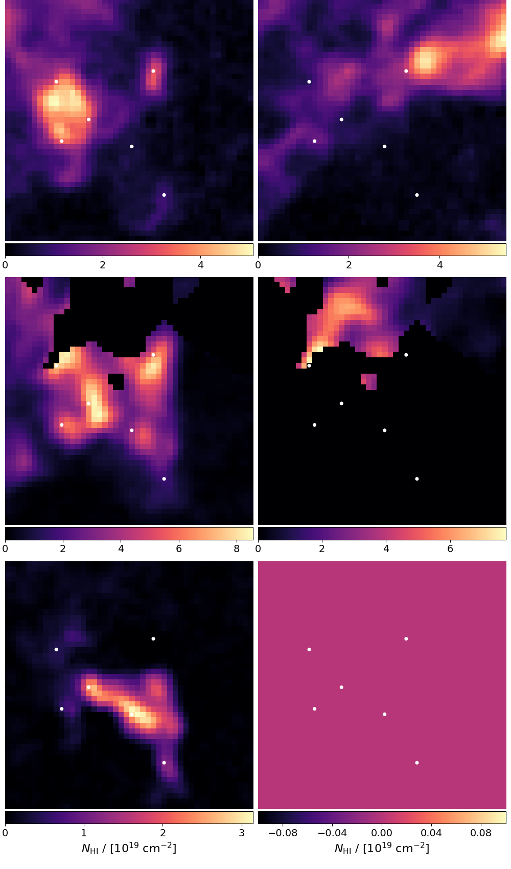
Figure 28: Column density maps of the six HVC phase components from ROHSA from N1 data, to be compared with the higher resolution Fig. 6 from EN data. (left): WNM_F (top), LNM_F (middle), which is actually quite warm (Table 1), and CNM_F (bottom); (right): WNM_A (top), LNM_A (middle), and CNM_A (bottom). Note that color bars have different scales. Coordinates (not shown here) are the same as in Fig. 2 (left). White circles indicate the positions of the six spectra shown in Fig. 4.

As summarized in Sect. 2.3.1, to evaluate the impact of the spatial resolution we performed a decomposition of N1 HVC spectra from the GHIGLS survey, using $N=6$ and all hyper-parameters equal to those used for the decomposition of the GHIGLS/N1 data. In this case, ROHSA also converges toward four components (Table 1). We applied the same procedure as for the DHIGLS/EN data to find the unstable and cold gas associated with regions F and A.

Figure 28 shows column density maps of the six phase components encoding the HVC in C I B (N1). Although at lower resolution here, phase structure as seen for the DHIGLS/EN data in Fig. 6 can be recognized. Importantly, the phase separation in region F shows evidence for cold gas (CNM_F), albeit at a somewhat higher velocity dispersion because of beam smearing (see Sect. 2.3.1, Table 1). On the other hand, the small amount of emission modeled in CNM_A using EN data is not present using N1 data (see lower right panel in Fig. 28).

Appendix B Segmentation of $N_{{\mathrm{H}}\,\mathrm{I}}$ maps using dendrograms

Using astrodendro we obtained a segmentation via hierarchical clustering in maps of $N_{{\mathrm{H}}\,\mathrm{I}}$ from EN data for WNM_F, LNM_F, and CNM_F, and for WNM_A, LNM_A, and CNM_A. To suppress noise, maps of WNM_F and WNM_A were convolved first to 4$\farcm$4, four times the native spatial resolution of EN data. For the six phases, Fig. 29 shows the structures obtained overlaid on the respective parent $N_{{\mathrm{H}}\,\mathrm{I}}$ map.

Table 6 summarizes the values of the three user-selected parameters. For each LNM and CNM phase these are the same: min_value, the threshold in $N_{{\mathrm{H}}\,\mathrm{I}}$ below which data are ignored, set at twice the sensitivity limit (see Table 2); min_delta, the minimum height in $N_{{\mathrm{H}}\,\mathrm{I}}$ required for a structure to be retained, set at the detection limit; and min_npix, the minimum number of pixels required for an independent structure, set at 16 pixels ($\sim 1.2$ times the size of the synthesized beam). Due to the convolution applied to WNM_F and WNM_A, lowering the sensitivity limits from those tabulated in Table 2, both min_value and min_delta were chosen manually to ensure a consistent visual clustering of the data. On finding the resulting clustering, the original WNM maps were used to infer the properties of the structures.

The convolution applied to WNM_F and WNM_A, to lower the noise, increases the size of the smallest structure that could be extracted. Although our methodology provides a realistic segmentation of the WNM maps, smaller warm structures ($<15$ pc) might be missed. However, such structures would be smaller than the larger unstable (LNM) structures extracted and their origin would more likely be attributed to turbulent cascade rather than thermal condensation.

Table 6: User parameters for astrodendro

	minvalue	mindelta	minnpix
	1019 cm-2	1019 cm-2
WNMF	0.5	0.5	16
LNMF	$2\times N_{{\mathrm{H}}\,\mathrm{I}}^{\rm lim}$	$N_{{\mathrm{H}}\,\mathrm{I}}^{\rm lim}$	16
CNMF	$2\times N_{{\mathrm{H}}\,\mathrm{I}}^{\rm lim}$	$N_{{\mathrm{H}}\,\mathrm{I}}^{\rm lim}$	16
WNMA	1	0.5	16
LNMA	$2\times N_{{\mathrm{H}}\,\mathrm{I}}^{\rm lim}$	$N_{{\mathrm{H}}\,\mathrm{I}}^{\rm lim}$	16
CNMA	$2\times N_{{\mathrm{H}}\,\mathrm{I}}^{\rm lim}$	$N_{{\mathrm{H}}\,\mathrm{I}}^{\rm lim}$	16

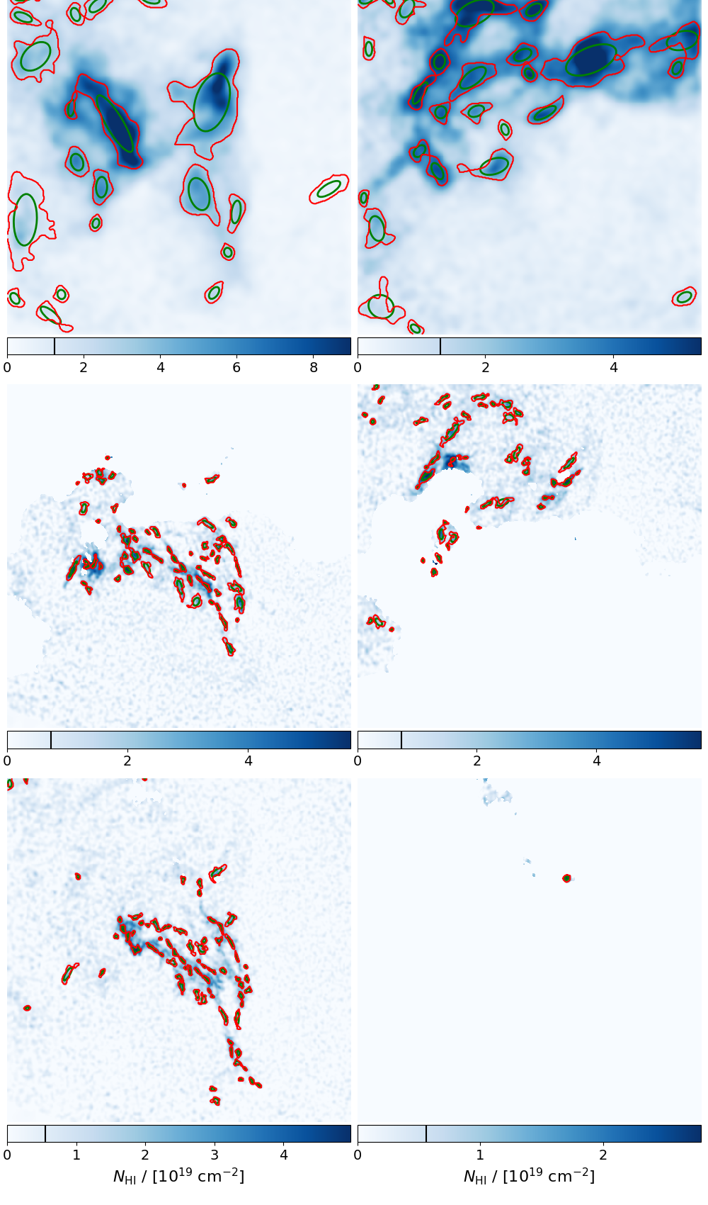
Figure 29: Structures extracted in the three HVC phases in each of two regions identified in C I B from EN using astrodendro. These are shown over the parent map of $N_{{\mathrm{H}}\,\mathrm{I}}$, as red contours over a blue color map (rather than that in Fig. 6) to highlight the clustering results. Corresponding ellipses are superimposed in green. (left): WNM_F (top), LNM_F (middle), and CNM_F (bottom); (right): WNM_A (top), LNM_A (middle), and CNM_A (bottom). The black mark on the color bars shows the sensitivity limits ($3\sigma$) tabulated in Table 2. For WNM_F and WNM_A, this has not been corrected for the convolution applied to suppress noise. Coordinates (not shown here) are the same as in Fig. 2 (left).

Appendix C Properties of structures from segmentation of $N_{{\mathrm{H}}\,\mathrm{I}}$ maps in environment A

Table 5 in Sect. 4.1 summarizes the results from the dendrogram analysis for region F. Here, for completeness and comparison, Table 7 provides a summary for region A.

Figure 30 shows the orientation of the dendrogram structures found for region A. In contrast to Fig. 13 for region F, where the preferred orientation was $+63\degree$, here the preferred orientation in almost orthogonal, $-43\degree$. The latter is interestingly similar to the orientation of the edge defined in Sect. 2.1 ($-60\degree$) and the arc of gas in WNM_A (Sect. 2.4).

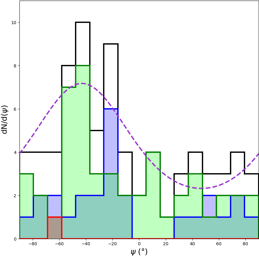
Figure 30: Probability distribution function of the position angle $\psi$ of each structure extracted from WNM_A (blue), LNM_A (green), and CNM_A (red). The total is shown in black. The purple dashed line shows the MLE fit of the Von Mises distribution to the orientations of all structures.

Table 7: Properties of structures in region A

	Symbol	WNMA	LNMA	CNMA	TotalA	Units
	$N_{c}$	26	48	1	75
Physical
Size	$L$	26 (1.5)	7.2 (1.5)	7.9 (1.0)	11.3 (2.1)	pc
Aspect ratio	$r$	1.7 (1.3)	2.0 (1.4)	1.1 (1.0)	1.9 (1.4)
Mass	$M_{{\mathrm{H}}\,\mathrm{I}}$	260 (2.6)	16 (2.3)	19 (1.0)	42 (4.9)	M⊙
Average number of H atoms per unit volume	$n$	0.41 (1.9)	1.21 (2.0)	1.1 (1.0)	0.84 (2.3)	cm-3
Thermodynamic
Doppler velocity dispersion	$\sigma_{T_{b}}$	9.8 (1.0)	3.1 (1.1)	2.1 (1.0)	4.6 (1.8)	km s-1
Turbulent velocity dispersion	$\sigma_{v_{z}}$	0.81 (2.5)	0.60 (2.0)	1.5 (1.0)	0.67 (2.2)	km s-1
Thermal velocity dispersion	$\sigma_{\rm th}$	9.7 (1.0)	2.9 (1.1)	1.4 (1.0)	4.4 (1.8)	km s-1
Kinetic temperature	$T_{k}$	11 (1.0)	1.0 (1.2)	0.24 (1.0)	2.4 (3.2)	103 K
Sound speed	$C_{s}$	11 (1.0)	3.2 (1.1)	1.6 (1.0)	4.8 (1.8)	km s-1
Thermal crossing time	$t_{\rm cross}^{\rm th}$	2.4 (1.5)	2.2 (1.6)	5.1 (1.0)	2.3 (1.6)	Myr
Turbulent crossing time	$t_{\rm cross}^{v_{z}}$	32 (2.1)	12 (1.8)	5.1 (1.0)	17 (2.2)	Myr
Thermal pressure	$P_{\rm th}/k_{B}$	4.8 (1.9)	1.3 (1.9)	0.3 (1.0)	2.0 (2.5)	103 K cm-3
Turbulent pressure	$P_{\rm v_{z}}/k_{B}$	0.1 (6.7)	0.2 (3.8)	1.0 (1.0)	0.1 (4.9)	101 K cm-3
Total pressure	$P_{\rm tot}/k_{B}$	5.6 (1.9)	1.7 (1.9)	1.3 (1.0)	2.6 (2.3)	103 K cm-3
Turbulent cascade
Turbulent sonic Mach number	$\mathcal{M}_{s}$	0.13 (2.5)	0.32 (2.0)	1.7 (1.0)	0.24 (2.5)
Mean free path	$\lambda$	0.78 (1.9)	0.27 (2.0)	0.30 (1.1)	0.39 (2.3)	10-3 pc
Kinematic molecular viscosity	$\nu$	1.1 (1.9)	0.11 (2.0)	0.06 (1.0)	0.24 (3.6)	1021 cm2 s-1
Knudsen number	$K_{n}$	3.0 (1.6)	3.7 (1.5)	3.7 (1.0)	3.4 (1.6)	10-5
Reynolds number	$Re$	0.56 (3.4)	1.1 (2.4)	5.8 (1.0)	0.89 (2.9)	104
Dissipation scale	$\eta$	4.1 (2.2)	0.68 (2.0)	0.21 (1.0)	1.2(3.1)	10-2 pc
Dissipation time	$t_{\eta}$	4.7 (3.8)	1.3 (2.6)	0.24 (1.0)	2.0 (3.6)	10-1 Myr
Convective time	$t_{L}$	35 (2.1)	13 (1.8)	6 (1.0)	18 (2.2)	Myr
Traversal time	$\tau_{L}$	36 (2.1)	13 (1.8)	6 (1.0)	18 (2.3)	Myr
Energy transfer rate	$\epsilon$	0.25 (12)	0.35 (6)	5.3 (1)	0.32 (8)	10-5 L⊙ M${}_{\odot}^{-1}$

Note. — Values correspond to the mean and spread from the logarithmic PDF.

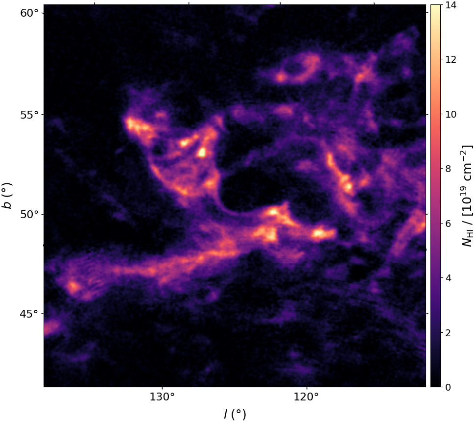
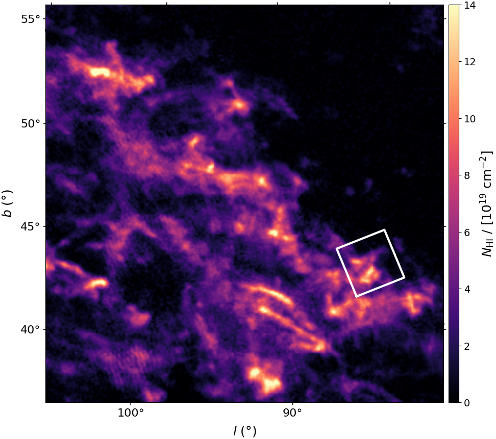
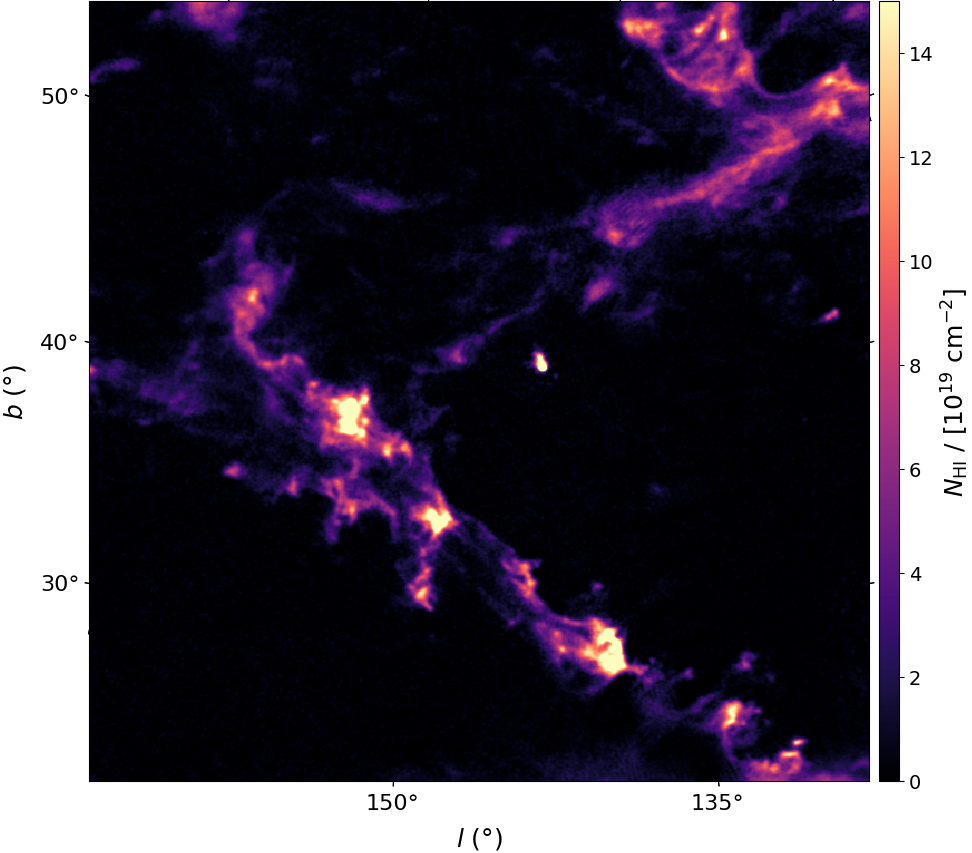
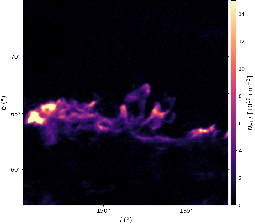
Figure 31: Zoomed images from Fig. 26 highlighting quasi-periodic scalloping and finger-like structures in $N_{{\mathrm{H}}\,\mathrm{I}}$ toward complex C and its neighbors. The apparent orientation of the features depends on the projection in the different maps. Top left: Emission toward the eastern end of complex C. Top right: Main body of complex C with its pronounced upper edge containing C I B (right). The white box shows the coverage selected from the EN data. Bottom left: Complex A and its bridge to complex C in the image above. Bottom right: The western part of complex M, adjacent to upper east end of complex C in projection.

Appendix D Deviation velocity

The deviation velocity for a given line of sight measures the difference between the observed $v_{\mathrm{LSR}}$ and the predicted velocities of H I  gas throughout a differentially-rotating model Galactic disk (Wakker, 1991). It can be used to identify gas in the halo that does not share the motion expected from the disk.

To evaluate the model, we used the rotation curve $v(R)$ at Galactocentric radius $R$ from the galpy “MWPotential2014” (Bovy, 2015) in

$$v_{\mathrm{LSR,\,model}}=\left(\frac{R_{0}}{R}v(R)-v\left(R_{0}\right)\right)\sin l\cos b\,.$$ (D1)

We adopted the simple model of the H I  disk from Wakker (2004), which has radius $R_{\rm{max}}$ = 26 kpc and flared edges $\pm z_{\max}$ in the vertical direction given by

$$z_{\max}=z_{1}\,\,(R<R_{0})\text{ and }z_{\max}=z_{1}+(z_{2}-z_{1})\times\frac{\left(R/R_{0}-1\right)^{2}}{4}\,\,(R>R_{0})\,,$$ (D2)

where $z_{1}$ and $z_{2}$ are 1 and 3 kpc, respectively. At any distance $d$ along the line of sight,

$$R=\sqrt{R_{0}^{2}+(d\cos b)^{2}-2R_{0}(d\cos b)\cos l}\text{ and }z=d\sin b\,.$$ (D3)

For any direction $(l,b)$, $v_{\mathrm{LSR,\,model}}$ can be evaluated using Eqs. D1 – D3 over the range of $d$ inside the model H I  disk ($R<R_{\rm{max}}$ and $|z|<z_{\max}$) to find the minimum and maximum, $v_{\rm{min,\,model}}$ and $v_{\rm{max,\,model}}$, respectively. The deviation velocity is defined as

$$v_{\mathrm{DEV}}=v_{\mathrm{LSR}}-v_{\rm{min,\,model}}\,(v_{\mathrm{LSR}}<0)\text{ and }v_{\mathrm{DEV}}=v_{\mathrm{LSR}}-v_{\rm{max,\,model}}\,(v_{\mathrm{LSR}}>0)\,.$$ (D4)

Appendix E Quasi-periodic scalloping and finger-like structures in complexes C, A, and M

In support of the discussion in Sect. 6.2, Fig. 31 shows $N_{{\mathrm{H}}\,\mathrm{I}}$ maps of the selected HVC emission from EBHIS for areas dominated by complex C and its neighbors, complexes A and M. The relative positions of the panels on the sky can be judged by using the coordinates on the axes, reference to Fig. 26 (albeit in a different projection), and the caption. These zoomed views highlight quasi-periodic scalloping and finger-like structures not only at obvious projected edges but also against the main body of gas, presumably because of projection of the complex boundary in 3D.

References

- Astropy Collaboration et al. (2013) Astropy Collaboration, Robitaille, T. P., Tollerud, E. J., et al. 2013, A&A, 558, A33
- Astropy Collaboration et al. (2018) Astropy Collaboration, Price-Whelan, A. M., Sipőcz, B. M., et al. 2018, AJ, 156, 123
- Audit & Hennebelle (2005) Audit, E., & Hennebelle, P. 2005, A&A, 433, 1
- Barger et al. (2012) Barger, K. A., Haffner, L. M., Wakker, B. P., et al. 2012, ApJ, 761, 145
- Barger et al. (2020) Barger, K. A., Nidever, D. L., Huey-You, C., et al. 2020, ApJ, 902, 154
- Blagrave et al. (2017) Blagrave, K., Martin, P. G., Joncas, G., et al. 2017, ApJ, 834, 126
- Bovy (2015) Bovy, J. 2015, ApJS, 216, 29
- Brüns et al. (2000) Brüns, C., Kerp, J., Kalberla, P. M. W., & Mebold, U. 2000, A&A, 357, 120
- Brunt et al. (2010) Brunt, C. M., Federrath, C., & Price, D. J. 2010, MNRAS, 405, L56
- Brüns et al. (2001) Brüns, C., Kerp, J., & Pagels, A. 2001, A&A, 370, L26
- Chandrasekhar (1961) Chandrasekhar, S. 1961, Hydrodynamic and hydromagnetic stability
- Chiappini et al. (2001) Chiappini, C., Matteucci, F., & Romano, D. 2001, ApJ, 554, 1044
- Cohen & Mirabel (1979) Cohen, R. J., & Mirabel, I. F. 1979, MNRAS, 186, 217
- Collins et al. (2003) Collins, J. A., Shull, J. M., & Giroux, M. L. 2003, ApJ, 585, 336
- Collins et al. (2007) —. 2007, ApJ, 657, 271
- Cram & Giovanelli (1976) Cram, T. R., & Giovanelli, R. 1976, A&A, 48, 39
- Danly et al. (1993) Danly, L., Albert, C. E., & Kuntz, K. D. 1993, ApJ, 416, L29
- Draine (1978) Draine, B. T. 1978, ApJS, 36, 595
- Encrenaz et al. (1971) Encrenaz, P. J., Penzias, A. A., Gott, R., I., Wilson, R. W., & Wrixon, G. T. 1971, A&A, 12, 16
- Field (1965) Field, G. B. 1965, ApJ, 142, 531
- Fox et al. (2004) Fox, A. J., Savage, B. D., Wakker, B. P., et al. 2004, ApJ, 602, 738
- Gaensler et al. (2008) Gaensler, B. M., Madsen, G. J., Chatterjee, S., & Mao, S. A. 2008, PASA, 25, 184
- Gibson et al. (2001) Gibson, B. K., Giroux, M. L., Penton, S. V., et al. 2001, AJ, 122, 3280
- Giovanelli & Haynes (1976) Giovanelli, R., & Haynes, M. P. 1976, MNRAS, 177, 525
- Giovanelli et al. (1973) Giovanelli, R., Verschuur, G. L., & Cram, T. R. 1973, A&AS, 12, 209
- Gong et al. (2017) Gong, M., Ostriker, E. C., & Wolfire, M. G. 2017, ApJ, 843, 38
- Goodman et al. (2009) Goodman, A. A., Rosolowsky, E. W., Borkin, M. A., et al. 2009, Nature, 457, 63
- Górski et al. (2005) Górski, K. M., Hivon, E., Banday, A. J., et al. 2005, ApJ, 622, 759
- Haffner et al. (2003) Haffner, L. M., Reynolds, R. J., Tufte, S. L., et al. 2003, ApJS, 149, 405
- Heitsch et al. (2016) Heitsch, F., Bartell, B., Clark, S. E., et al. 2016, MNRAS, 462, L46
- Hennebelle & Audit (2007) Hennebelle, P., & Audit, E. 2007, A&A, 465, 431
- Hennebelle & Pérault (1999) Hennebelle, P., & Pérault, M. 1999, A&A, 351, 309
- Hennebelle & Pérault (2000) —. 2000, A&A, 359, 1124
- Hsu et al. (2011) Hsu, W. H., Putman, M. E., Heitsch, F., et al. 2011, AJ, 141, 57
- Hulsbosch (1968) Hulsbosch, A. N. M. 1968, Bull. Astron. Inst. Netherlands, 20, 33
- Hulsbosch & Raimond (1966) Hulsbosch, A. N. M., & Raimond, E. 1966, Bull. Astron. Inst. Netherlands, 18, 413
- Hunter (2007) Hunter, J. D. 2007, CSE, 9, 90
- Kalberla & Haud (2006) Kalberla, P. M. W., & Haud, U. 2006, A&A, 455, 481
- Kalberla & Haud (2015) Kalberla, P. M. W., & Haud, U. 2015, A&A, 578, A78
- Kalberla et al. (1999) Kalberla, P. M. W., Kerp, J., & Haud, U. 1999, \aspconf, Vol. 166, HVCs Probing a Gaseous Galactic Halo, ed. B. K. Gibson & M. E. Putman, 155
- Kalberla et al. (2010) Kalberla, P. M. W., McClure-Griffiths, N. M., Pisano, D. J., et al. 2010, A&A, 521, A17
- Kerp et al. (1999) Kerp, J., Burton, W. B., Egger, R., et al. 1999, A&A, 342, 213
- Kerp et al. (2011) Kerp, J., Winkel, B., Ben Bekhti, N., Flöer, L., & Kalberla, P. M. W. 2011, Astronomische Nachrichten, 332, 637
- Kim & Ryu (2005) Kim, J., & Ryu, D. 2005, ApJLetters, 630, L45
- Kolmogorov (1941) Kolmogorov, A. 1941, Akademiia Nauk SSSR Doklady, 30, 301
- Kunth et al. (1994) Kunth, D., Lequeux, J., Sargent, W. L. W., & Viallefond, F. 1994, A&A, 282, 709
- Kuntz & Danly (1996) Kuntz, K. D., & Danly, L. 1996, ApJ, 457, 703
- Lequeux (2012) Lequeux, J. 2012, Le Milieu interstellaire, SAVOIRS ACTUELS (EDP Sciences)
- Lockman et al. (2008) Lockman, F. J., Benjamin, R. A., Heroux, A. J., & Langston, G. I. 2008, ApJ, 679, L21
- Marasco & Fraternali (2011) Marasco, A., & Fraternali, F. 2011, A&A, 525, A134
- Marchal & Miville-Deschênes (2021) Marchal, A., & Miville-Deschênes, M.-A. 2021, ApJ, 908, 186
- Marchal et al. (2019) Marchal, A., Miville-Deschênes, M.-A., Orieux, F., et al. 2019, A&A, 626, A101
- Martin et al. (2015) Martin, P. G., Blagrave, K. P. M., Lockman, F. J., et al. 2015, ApJ, 809, 153
- McClure-Griffiths et al. (2009) McClure-Griffiths, N. M., Pisano, D. J., Calabretta, M. R., et al. 2009, ApJS, 181, 398
- Miville-Deschênes et al. (2017) Miville-Deschênes, M.-A., Salomé, Q., Martin, P. G., et al. 2017, A&A, 599, A109
- Muller et al. (1963) Muller, C. A., Oort, J. H., & Raimond, E. 1963, Academie des Sciences Paris Comptes Rendus, 257, 1661
- Ossenkopf et al. (2006) Ossenkopf, V., Esquivel, A., Lazarian, A., & Stutzki, J. 2006, A&A, 452, 223
- Peek et al. (2011) Peek, J. E. G., Heiles, C., Douglas, K. A., et al. 2011, ApJS, 194, 20
- Peek et al. (2018) Peek, J. E. G., Babler, B. L., Zheng, Y., et al. 2018, ApJS, 234, 2
- Putman et al. (2003) Putman, M. E., Bland-Hawthorn, J., Veilleux, S., et al. 2003, ApJ, 597, 948
- Putman et al. (2012) Putman, M. E., Peek, J. E. G., & Joung, M. R. 2012, ARA&A, 50, 491
- Putman et al. (2002) Putman, M. E., de Heij, V., Staveley-Smith, L., et al. 2002, AJ, 123, 873
- Reynolds (1883) Reynolds, O. 1883, Philosophical Transactions of the Royal Society of London, 174, 935
- Rosolowsky et al. (2008) Rosolowsky, E. W., Pineda, J. E., Kauffmann, J., & Goodman, A. A. 2008, ApJ, 679, 1338
- Ryans et al. (1997a) Ryans, R. S. I., Keenan, F. P., Sembach, K. R., & Davies, R. D. 1997a, MNRAS, 289, 986
- Ryans et al. (1997b) —. 1997b, MNRAS, 289, 83
- Thom et al. (2008) Thom, C., Peek, J. E. G., Putman, M. E., et al. 2008, ApJ, 684, 364
- Tielens & Hollenbach (1985) Tielens, A. G. G. M., & Hollenbach, D. 1985, ApJ, 291, 722
- Tripp et al. (2003) Tripp, T. M., Wakker, B. P., Jenkins, E. B., et al. 2003, AJ, 125, 3122
- Tufte et al. (1998) Tufte, S. L., Reynolds, R. J., & Haffner, L. M. 1998, ApJ, 504, 773
- van der Walt et al. (2011) van der Walt, S., Colbert, S. C., & Varoquaux, G. 2011, CSE, 13, 22
- van Woerden et al. (1999) van Woerden, H., Schwarz, U. J., Peletier, R. F., Wakker, B. P., & Kalberla, P. M. W. 1999, Nature, 400, 138
- Wakker et al. (1996) Wakker, B., Howk, C., Schwarz, U., et al. 1996, ApJ, 473, 834
- Wakker (1991) Wakker, B. P. 1991, A&A, 250, 499
- Wakker (2001) Wakker, B. P. 2001, ApJS, 136, 463
- Wakker (2004) Wakker, B. P. 2004, Astrophysics and Space Science Library, Vol. 312, HVC/IVC Maps and HVC Distribution Functions, ed. H. van Woerden, B. P. Wakker, U. J. Schwarz, & K. S. de Boer, 25
- Wakker & Schwarz (1991) Wakker, B. P., & Schwarz, U. J. 1991, A&A, 250, 484
- Wakker & van Woerden (1991) Wakker, B. P., & van Woerden, H. 1991, A&A, 250, 509
- Wakker et al. (1999) Wakker, B. P., Howk, J. C., Savage, B. D., et al. 1999, Nature, 402, 388
- Wakker et al. (2003) Wakker, B. P., Savage, B. D., Sembach, K. R., et al. 2003, ApJS, 146, 1
- Wakker et al. (2007) Wakker, B. P., York, D. G., Howk, J. C., et al. 2007, ApJ, 670, L113
- Wang et al. (2005) Wang, Q. D., Yao, Y., Tripp, T. M., et al. 2005, ApJ, 635, 386
- Weiner & Williams (1996) Weiner, B. J., & Williams, T. B. 1996, AJ, 111, 1156
- Winkel et al. (2016) Winkel, B., Kerp, J., Flöer, L., et al. 2016, A&A, 585, A41
- Woerden et al. (2004) Woerden, H. v., Wakker, B., Schwarz, U., & Boer, K. d. 2004, High-Velocity Clouds (Springer Science & Business Media)
- Wolfire et al. (1995a) Wolfire, M. G., Hollenbach, D., McKee, C. F., Tielens, A. G. G. M., & Bakes, E. L. O. 1995a, ApJ, 443, 152
- Wolfire et al. (1995b) Wolfire, M. G., McKee, C. F., Hollenbach, D., & Tielens, A. G. G. M. 1995b, ApJ, 453, 673
- Wolfire et al. (2003) —. 2003, ApJ, 587, 278
- Yao et al. (2011) Yao, Y., Shull, J. M., & Danforth, C. W. 2011, ApJ, 728, L16