Fast, high-fidelity Lyman $\alpha$ forests with convolutional neural networks

Abstract

Full-physics cosmological simulations are powerful tools for studying the formation and evolution of structure in the universe but require extreme computational resources. Here, we train a convolutional neural network to use a cheaper N-body-only simulation to reconstruct the baryon hydrodynamic variables (density, temperature, and velocity) on scales relevant to the Lyman-$\alpha$ (Ly$\alpha$) forest, using data from Nyx simulations. We show that our method enables rapid estimation of these fields at a resolution of $\sim$20kpc, and captures the statistics of the Ly$\alpha$ forest with much greater accuracy than existing approximations. Because our model is fully-convolutional, we can train on smaller simulation boxes and deploy on much larger ones, enabling substantial computational savings. Furthermore, as our method produces an approximation for the hydrodynamic fields instead of Ly$\alpha$ flux directly, it is not limited to a particular choice of ionizing background or mean transmitted flux.

1 Introduction

Understanding the distribution and evolution of the matter in the universe is at the core of modern cosmology and a main motivation for the upcoming generation of astronomical surveys. But to extract cosmological insights, observations have to be compared to theoretical predictions for different cosmological scenarios. Predicting observable quantities in general, and Ly$\alpha$ forest specifically, from the underlying large scale structure is complicated by the nonlinear mapping between baryons (responsible for most of observables) and dark matter (which dominates the gravitational dynamics). In the early days preceding “precision cosmology”, simplified models were successfully used, for example baryons-trace-dark-matter approximation (Petitjean et al., 1995), or modifying the matter density field (Gnedin & Hui, 1996) or gravitational potential (Gnedin & Hui, 1998), to mimic the effects of baryonic pressure smoothing. The gas temperature of the intergalacic medium (IGM) in those models is usually computed by imposing a polytropic temperature–density relation (Hui & Gnedin, 1997).

More recently, recipes to model Ly$\alpha$ forest without running full hydrodynamical simulations have been provided by Peirani et al. (2014) and Sorini et al. (2016), as well as models for specific summary statistics in Seljak (2012), but they have not been really used in practice due to their complexity and/or applicability to only a limited range of scales. Thus, Ly$\alpha$ forest forward models rely on computationally expensive hydrodynamical simulations (Iršič et al., 2017; Boera et al., 2019; Walther et al., 2019; Palanque-Delabrouille et al., 2020; Rogers & Peiris, 2020; Walther et al., 2021), and solving inverse problems commonly requires running dozens of simulations, at a rough cost of 2 million CPU hours per simulation (see, for example, Walther et al., 2021). Of course, if one wants to consider cosmological models beyond standard $\Lambda$CDM or to model complex astrophysical phenomena affecting the Ly$\alpha$ signal like high column density absorbers (Rogers et al., 2018), UV background fluctuations (Oñorbe et al., 2019), or HeII reionization (Upton Sanderbeck & Bird, 2020) the number of needed simulations, and thus the computational costs, will increase significantly. Such applications present a clear need for surrogate models which can mitigate some of the cost of running full-fledged hydrodynamic simulations for every test case.

Beyond generation of mock catalogs and hydrodynamic emulators, there is also a growing need for fast hydrodynamical mapping in the context of differentiable forward model reconstructions (Horowitz et al., 2019). There, the underlying matter distribution is reconstructed under constraints from gravitational evolution and using, for example, the three dimensional Ly$\alpha$ tomographic reconstructions under the Fluctuating Gunn-Peterson Approximation (FGPA; Gunn & Peterson (1965)) as done in Horowitz et al. (2019); Porqueres et al. (2019); Horowitz et al. (2020). Reducing the modeling cost via fast and efficient — even if approximate — methods of reproducing the Ly$\alpha$ signal is thus of significant interest to the community. Our paper addresses this issue using data-driven modeling trained on hydrodynamical simulations.

In recent years, deep neural networks (NN) have become a promising method to assist in solving these highly nonlinear problems, by acting as surrogate models (which are differentiable by design) for complex phenomena. In particular, Generative Adversarial Networks (Goodfellow et al. 2014; GANs) and U-Nets (Ronneberger et al., 2015) have proven useful in a variety of cosmology tasks that either directly generate synthetic hydrodynamic quantities (Zamudio-Fernandez et al., 2019), or reconstruct them from dark matter distributions. The latter approach allows one to run cheaper N-body simulations (or even surrogates for N-body evolution) to generate a dark matter distribution, then rapidly estimate the target hydrodynamic quantity corresponding to the dark matter structure. In the context of the thermal and kinematic Sunyaev-Zel’dovich effects, this approach has been shown to be useful in reconstructing electron density, presssure, and momenta in 3D (Thiele et al., 2020) as well as gas pressure in 2D (Tröster et al., 2019). These works showcase the success of neural networks in producing hydrodynamic fields with superior statistical fidelity compared to competing classical or semi-analytical methods. While extremely promising, deep learning approaches are data-hungry, and require generation of training data at the desired output resolution (e.g., $\sim$100 kpc in Thiele et al. 2020) to achieve maximal model fidelity. It is thus important to maintain a reasonable volume of training data when extending such models to finer-scale hydrodynamic reconstruction, and investigate the data needs in such regimes.

In this work, we use neural networks to reconstruct 3D baryon hydrodynamics from N-body dark matter simulations at $\sim$20 kpc/$h$ resolution, roughly an order of magnitude finer than previous neural hydrodynamic reconstructions. Given a snapshot of dark matter, our model allows rapid estimation of baryon density, temperature, and velocity fields, which can be painted in over an arbitrarily large volume at the given resolution.

The paper is organized as follows. We first describe the simulation data used to train our model and detail how we compute FGPA estimates and Ly$\alpha$ forest quantities in Section 2. Then, we describe the model design and training process in Section 3. Our results are presented in Section 4, where we show sample output from our model and make statistical comparisons against the true hydrodynamic fields. Finally, we present conclusions and discussion in Section 5.

2 Simulations

We construct our training and validation datasets from pairs of cosmological simulations run with the Nyx code (Almgren et al., 2013; Lukić et al., 2015). Each pair of simulations share identical initial conditions and cosmology, with one simulation modeling the full-physics problem (dark matter particle N-body dynamics as well as baryon hydrodynamics), while the other just models the evolution of dark matter particles (N-body-only). In Nyx, the dark matter particles are evolved with a particle-mesh scheme, while the additional baryon hydrodynamics are modeled as an inviscid ideal fluid on a set of Eulerian grids. We neglect physics related to galaxy formation, but this is extremely common approach in Ly$\alpha$ cosmological simulations (Iršič et al., 2017; Boera et al., 2019; Walther et al., 2019; Rogers & Peiris, 2020; Walther et al., 2021; Pedersen et al., 2020). This is because regions transparent to Ly$\alpha$ photons at redhisfts $z\gtrsim 2$ are in low density regions (Lukić et al., 2015; McQuinn, 2016), and poorly understood physical processes related to galaxy formation only play a minor role in those regions (Kollmeier et al., 2006; Desjacques et al., 2006).

With this paired dataset, we can train our model to learn a mapping from the cheaper N-body-only simulation into the hydrodynamic fields of the full-physics simulation in a supervised fashion. We use one pair of simulations for training, and an independent pair, with identical cosmology but different initial conditions, for validation. For both the training and validation pairs of simulations, the cosmological parameters are $\Omega_{b}=0.05$, $\Omega_{M}=0.31$, $\Omega_{L}=0.69$, and $h=0.675$. The physical fields of interest are defined on a 3D uniform $1024^{3}$ grid, spanning a cube of $L=20$ Mpc/$h$ per side, with periodic boundary conditions. For the hydrogen and helium mass abundances we adopted values consistent with the CMB observations and Big Bang nucleosynthesis (Coc et al., 2013): $X_{p}$=0.76 and $Y_{p}$=0.24. Dark matter N-body dynamics are evolved with $1024^{3}$ particles, then density and velocities are deposited on the grid using Cloud-In-Cell (CIC) interpolation. We select the $z=3$ snapshot in each simulation for training and validation, as it lies in the center of the range of redshifts most relevant for Ly$\alpha$ analysis.

Data scales in Nyx files can span many orders of magnitude, so we normalize the data to order unity for training stability. For all velocity fields, we scale linearly to $\mathbf{\hat{v}}=\mathbf{v}/(9\times 10^{7}\,\mathrm{cm}\cdot\mathrm{s}^{-1})$. The baryon density and temperature fields have a large dynamic range, so we use

$$\hat{\rho} =\log(\rho/14),$$

$$\hat{T} =\log(T)/8-1.5,$$ (1)

$$\hat{\rho}_{DM} =\log(1+\rho_{DM})/12.$$

where $\rho$ and $T$ are the baryon overdensity and temperature (in Kelvin), respectively, while $\rho_{DM}$ is the overdensity of dark matter. All network outputs are transformed back into their original units before performing analysis or validation on statistical quantities.

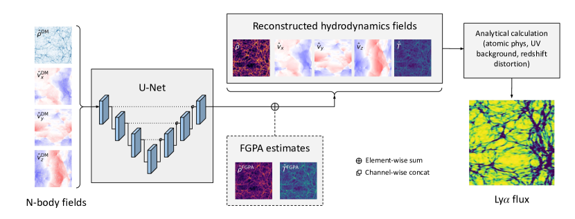
Figure 1: Schematic depicting our model, which predicts the hydrodynamic fields from an input n-body simulation. We train separate networks for $\hat{\rho}$, $\hat{T}$, and $\mathbf{\hat{v}}=(\hat{v}_{x},\hat{v}_{y},\hat{v}_{z})$, and for $\hat{\rho}$ and $\hat{T}$ we predict the correction to the FGPA approximations $\hat{\rho}^{\mathrm{FGPA}},\hat{T}^{\mathrm{FGPA}}$ rather than the full fields. As the model reconstructs the raw hydrodynamic fields, it is independent of Ly$\alpha$-specific physical details.

2.1 FGPA estimates

The long-standing method to reconstruct hydrodynamic quantities for purposes of Ly$\alpha$ modeling is the FGPA (Gunn & Peterson, 1965; Sorini et al., 2016)). This procedure takes the dark matter overdensity $\rho^{DM}$ from the N-body simulation, with or without artificial smoothing, to produce estimates for the baryon density $\rho$ and temperature $T$, given by a power law relation (Hui & Gnedin, 1997)

$$T=T_{0}(\rho/\langle\rho\rangle)^{\gamma-1}\,,$$ (2)

where $\langle\rangle$ denotes averaging over volume. The estimate for $\rho$ is usually attained by applying Gaussian smoothing (with smoothing length $\lambda_{G}$ roughly given by the Jeans filtering scale) to $\rho^{\mathrm{DM}}$ to simulate baryonic pressure smoothing. In this work, we empirically determine the best-fit $T_{0}$, $\gamma$, and $\lambda_{G}$ for our simulation. We best-fit Gaussian smoothing scale using least square differences between the smoothed dark matter density from the N-body simulation and the actual baryon density field from the hydrodynamical simulation. We then fit density and temperature in the hydrodynamical simulations to the power-law relation in eq. 2 as described in Lukić et al. (2015), arriving for our particular simulation and redshift $z=3$, to values:

$$T_{0} =12,300\,\text{K}$$

$$\gamma =1.49$$ (3)

$$\lambda_{G} =43.5\,\text{kpc}/h.$$

We use these values to compute FGPA estimates for the hydrodynamic fields in the test simulation and use the resulting Ly$\alpha$ flux as a baseline to compare against the accuracy of our neural network approach. Additionally, FGPA is a useful starting point for the neural network training process, providing an initial guess upon which the network can improve.

2.2 Lyman $\alpha$ computation

Given the true or estimated baryon hydrodynamics fields, we can then compute Ly$\alpha$ flux analytically. We use the Gimlet code (Friesen et al., 2016) to do this step. We compute the optical depth, $\tau$, of neutral Hydrogen at a fixed redshift, which is related to the transmitted flux fraction with: $F=\exp{(-\tau)}$. We do not account for the finite speed of light when we cast rays in the simulation, but we use the thermodynamical state of baryons at a fixed cosmic time. The simulated spectra are thus not meant to fully reproduce observed Ly$\alpha$ forest spectra, but to recover the flux statistics in a given redshift window. Our calculation of the spectra accounts for Doppler shifts due to bulk flows of the gas and for the thermal broadening of the Ly$\alpha$ line. We have neglected noise and metal contamination, but this is both common procedure in the field, and is not relevant for this paper. We refer to Lukić et al. (2015) for specific details of these calculations. Finally, we rescale the UV background intensity so that the mean flux of all spectra from the network model predictions and hydrodynamical simulation match. Note that with our neural networks we predict the hydrodynamic fields ($\rho$, $T$, $\bf{v}$) directly, thus we use identical pipelines and assumptions when calculating Ly$\alpha$ forest quantities from Nyx simulations and NN models. This makes our approach orthogonal to any particular choices made in modeling Ly$\alpha$ forest from basic thermodynamical quantities.

3 Model Design

As the target baryon hydrodynamical fields each have their own unique features, we partition the problem and train one generator network each for $\hat{\rho}$, $\hat{T}$, and $\mathbf{\hat{v}}$. We use the same U-Net architecture for our generation networks, as this design is efficient in extracting high-level features through sequential downsampling, while maintaining the ability to resolve fine-grained details via skip connections. The fully-convolutional nature of the U-Net allows us to train on smaller sub-volumes and then predict on larger volumes without issue.

3.1 Network architecture

Each downsampling block in our U-Nets consists of a 3D convolution with stride 2, followed by a leaky ReLU activation (Maas et al., 2013). There are a total of 6 downsampling blocks, and a corresponding 6 upsampling blocks. Each upsampling block consists of a 3D transposed convolution with stride 1/2, followed by a ReLU activation (Nair & Hinton, 2010), except the final upsampling convolution, which has a $\tanh$ nonlinearity. After each upsampling block, the incoming skip connections from the corresponding downsampling block are concatenated to the features along the channel axis.

The input to the network consists of the normalized dark matter density and velocity fields $(\hat{\rho}^{DM},\hat{v}^{DM}_{x},\\ \hat{v}^{DM}_{y},\hat{v}^{DM}_{z})$, which are supplied as different feature channels over a 3D volume. During training, we generate samples by randomly cropping sub-volumes from the training simulations. The crop size is a tunable hyperparameter, and we find best performance with crops of size $128^{3}$ for the density and temperature fields, and $256^{3}$ for the velocity fields. As additional augmentations, we randomly apply rotations and transposes from the octahedral group to these training samples. Together, the random crops and rotations implicitly enforce the large-scale homogeneity and isotropy of the universe, and help extend the utility of our single pair of training simulations.

For the baryon density and temperature targets, we observe a performance benefit when incorporating the FGPA estimates into the training workflow, as depicted in Figure 1. In this setup, the network predictions are added to the FGPA estimate to produce the final field, so the model is trained to predict a correction term to the FGPA estimate rather than the full hydrodynamic field at once. This accelerates convergence and improves the statistical fidelity of our final fields.

3.2 Loss functions

The main component of our loss function is the $\mathcal{L}_{1}$ distance between the generated and target fields. The velocity U-Net is trained entirely with this loss function, but for the baryon density and temperature fields we observe an inability to adequately capture high-density/temperature features training only with $\mathcal{L}_{1}$ loss. This is consistent with the well-known tendency of $\mathcal{L}_{1}$ to seek a conservative (maximum-likelihood) estimate and average over fine-scale features, causing noticeable blurring in the network output (Isola et al., 2016).

Thus, for the density and temperature fields we also employ an adversarial loss, given by a discriminator $D$. Contrary to a standard adversarial setup, our discriminator operates in Fourier space rather than the original data space. This is motivated by the observation that taking a sample (cube with side length $N$) and removing the $N/2$ smallest-scale Fourier modes along each axis retains much of the important detail, while reducing dimensionality by a roughly an order of magnitude (a factor of 2 along each dimension). With our large 3D training samples, this reduction of dimensionality helps compensate for the added overhead of training an additional discriminator network.

We thus use the following procedure when training our spectral discriminator $D$. The discriminator’s input fields $x$ are crops (with side length $N=128$) of the baryon density or temperature field, coming from either the training simulation or our generator network. We compute the discrete Fourier transform of these crops (with wavenumbers $\{-N/2,...,0,...,N/2-1\}$) along each dimension, then drop modes with $|k|>=N/4$ to get the truncated Fourier transform $\tilde{x}_{t}$. Then, we feed the truncated Fourier coefficients $f=\tilde{x}_{t}\tilde{x}^{*}_{t}$ to the spectral discriminator, which tries to classify the sample as real or fake. Our discriminator has four downsampling convolutional layers, followed by three fully-connected layers which end in a single output classifying the input as real or fake. To give the spectral discriminator additional context, we concatenate the dark matter density input as an additional feature channel before applying the Fourier truncation.

Following the standard non-saturating GAN formulation (Goodfellow et al., 2014), the adversarial loss for the discriminator is

$$\mathcal{L}_{D}=-\log D(f_{\rm{real}})-\log(1-D(f_{\rm{fake}})),$$ (4)

while the total loss for the $\hat{\rho}$ and $\hat{T}$ U-Nets is

$$\mathcal{L}_{\mathrm{U\mathchar 45\relax Net}}=\lambda\mathcal{L}_{1}+\log D(f_{\rm{fake}}),$$ (5)

where $\lambda=500$ is a hyperparameter to up-weight the importance of the $\mathcal{L}_{1}$ loss.

4 Results

We evaluate the accuracy of our approach primarily by comparing the PDF (Rauch et al., 1997) and 1D power spectra (Croft et al., 1999) of our model’s Ly$\alpha$ fields against those of the test simulation. The Ly$\alpha$ flux variation along some line-of-sight axis is defined with respect to fluctuations about the global mean $\bar{F}$, as $\delta_{F}=(F-\bar{F})/\bar{F}$. From this, the 1D power spectrum $P(k)$ is given by

$$P(k)=\langle\widetilde{\delta}_{F}(k)\widetilde{\delta}^{*}_{F}(k)\rangle,$$ (6)

where $\widetilde{\delta}_{F}(k)$ is the Fourier transform of $\delta_{F}$ and the mean $\langle\rangle$ is taken over all modes with magnitude $k$ along the given line-of-sight axis (one flux skewer per spatial location $i,j$). From this we can compute the transfer function $T(k)$, defined by

$$T(k)=\sqrt{\frac{P^{\mathrm{U\mbox{-}Net}}(k)}{{P^{\mathrm{True}}(k)}}},$$ (7)

to assess how closely our predicted Ly$\alpha$ fields match the test simulation in power spectra.

During training, candidate models are selected based on how closely their hydrodynamic reconstructions for $\hat{\rho}$, $\hat{T}$, and $\mathbf{\hat{v}}$ match the PDFs of the ground truth fields. Then, the hydrodynamic reconstruction is computed for the entire test simulation at once by applying our network to the full 1024³ volume, using periodic padding to enforce the periodic boundary conditions. We choose our final model based on the accuracy of the PDF and $P(k)$ for the Ly$\alpha$ fields computed from the hydrodynamic reconstruction. In the following sections we will visualize our Ly$\alpha$ and corresponding hydrodynamic fields, and detail how closely they mach the test simulation in the summary statistics. We compare against the FGPA Ly$\alpha$ estimates as a baseline. Then, we will analyze the hydrodynamic reconstructions and examine some failure modes.

4.1 Lyman $\alpha$ fields

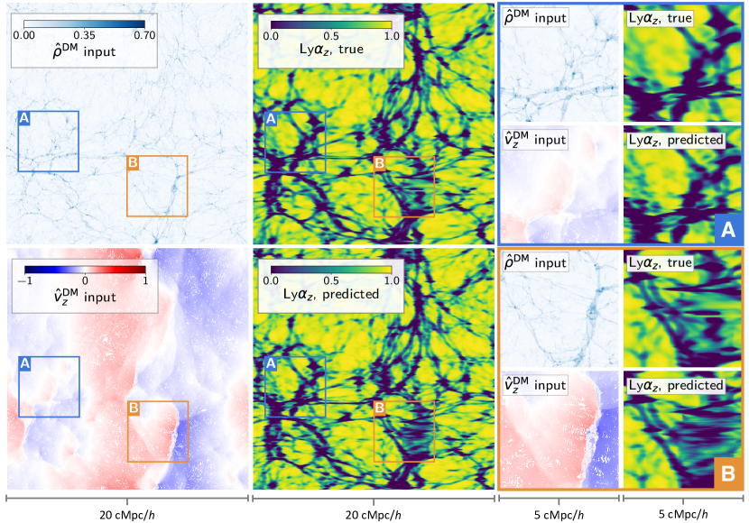
Figure 2: Slices of the test simulation, with the true and predicted Ly$\alpha$ fields along the $z$-axis line-of-sight. At left, we show a slice through the full volume of the input dark matter density and the line-of-sight dark matter velocity $v_{z}$ for reference. The corresponding true and predicted Ly$\alpha_{z}$ fields for this slice are shown in the center panels, and at left we show zoom-ins to regions A and B to better contrast our model against the ground truth.

A visualization of our results is shown in Figure 2, where we render some of the input fields and corresponding Ly$\alpha$ fields at a randomly chosen slice in the $x$-$z$ plane ($z$ was chosen as the line-of-sight here). The slices run the entire length of the simulation box, but several zoomed-in regions are also shown for increased detail on the right-hand side.

The predicted Ly$\alpha$ field has a high degree of visual fidelity, and closely matches the ground truth in diffuse IGM regions where densities are lower or where there is not much gas motion (see zoom-in panel A). By contrast, regions where gas is collapsing onto a filament structure show more of a discrepancy (zoom-in panel B), as the redshift distortion from the velocity field effectively stretches the size of the filament in the redshifted Ly$\alpha$ field and amplifies any discrepancies between the true and reconstructed hydrodynamic fields along the filament. In general, dense filaments and clusters make up an exceedingly small fraction of the total volume, so the model has more difficulty capturing the fine-scale features in these regions due to limited training examples.

Since at $z=3$ the Ly$\alpha$ transmission drops to zero at overdensity of a few (see Fig. 7 in Lukić et al. (2015)), we can still obtain statistically accurate Ly$\alpha$ fields from our hydrodynamic reconstructions without necessarily capturing the full range of scales in the gas physics. This is demonstrated in Figure 3, where we show the PDF and 1D power spectrum of our Ly$\alpha$ estimates and compare against the ground truth. We compute the metrics for Ly$\alpha$ fields with lines-of-sight along all three axes of our box, and plot the mean, minimum and maximum per $F$ and $k$ bin across the three fields.

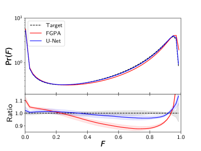
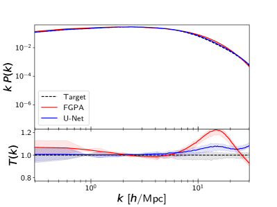
Figure 3: The PDF (left) and power spectrum (right) of full-volume Ly$\alpha$ flux fields from our model and FGPA, compared against the test simulation. Lines and shaded regions represent the mean and min/max per bin across Ly$\alpha$ fields with lines of sight along the $x$, $y$, and $z$ axes.

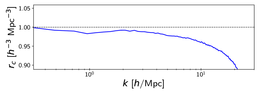
Figure 4: The cross-correlation coefficient $r_{c}$ of our predicted Ly$\alpha$ field over the relevant length scales. We used the $z$-axis line-of-sight for this plot.

In both statistical measures, the Ly$\alpha$ estimates from our model are within a few percent of the ground truth across the relevant $F$ and $k$ bins, significantly improving on the FGPA Ly$\alpha$ estimates. Our model begins to accumulate an excess of power in $P(k)$ near $k\sim 10$ $h$/Mpc, as does FGPA. Beyond 10 $h$/Mpc, both our model and FGPA begin to diverge from the truth, with our model having an excess of power at high wavenumbers while FGPA diverges in the other direction. However, $k\sim 10$ $h$/Mpc is typically the highest mode considered in Ly$\alpha$ spectroscopic studies, limited by contamination from metal lines (see Sorini et al. 2016 and references therein), so we truncate the plot near that wavenumber and do not consider the discrepancies beyond it to be detrimental to our approach.

To further evaluate our model, we compute the cross correlation coefficient $r_{c}$ , defined as

$$r_{c}=\frac{P_{rt}}{\sqrt{P_{rr}P_{tt}}},$$ (8)

where $P_{rt}$ is the cross-power and $P_{rr},P_{tt}$ are the auto-power of the reconstructed and true Ly$\alpha$ fields, respectively. The cross-correlation for the $z$-axis line-of-sight is shown in Figure 4. We see good agreement, with $r_{c}>0.95$ across the relevant $k$ range.

4.2 Hydrodynamic fields

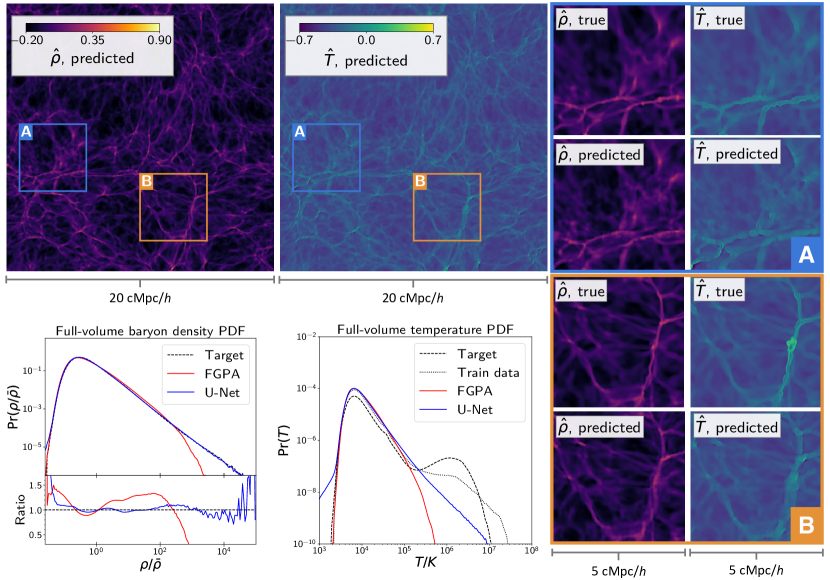
Figure 5: Predicted baryon density and temperature fields, sliced at the same location as plotted in Figure 2. In the right-side panels we show zoom-ins to regions A and B as before. In the lower-left panels, we plot the full-volume PDFs for these fields (after transforming back to original simulation units) compared to the ground truth and FGPA. The reconstructed baryon density field has captured the full range of scales to within $\sim 10\%$, while the temperature field has overfit to the distribution of the train simulation, which differs significantly from the test simulation.

Inspecting the direct output of our model, the hydrodynamic fields, gives more insight into the difficulty of our task. In Figure 5, we visualize slices of the density and temperature fields at the same location as in Figure 2, comparing our reconstructions against the ground truth fields. While there is good agreement by eye, the zoomed-in panels show discrepancies between the true and generated fields, particularly in how sharply resolved the edges of filament structures are. There are also some small-scale artifacts, especially in the temperature field, which possibly contribute to the excess of power seen at small scales in the Ly$\alpha$ $P(k)$.

In the lower left panels, we also plot the PDFs of the two fields, computed over the entire 1024³ volume of the test simulation. The full-volume PDF for the density field actually shows remarkable agreement between our model’s reconstruction and the true field, with the full range of scales captured to within $\sim 10\%$. This is in contrast to FGPA, which completely fails in estimating densities beyond $(\rho/\bar{\rho})\gtrsim 10^{3}$.

In the temperature field, the reconstructions from FGPA and our model both differ significantly from the truth. For reference, we have also plotted the full-volume PDF of the temperature field from the training simulation, and we see that FGPA and our model both closely track the train distribution for $T/K<10^{5}$, indicating overfitting. However, there is a clear distributional difference between the train and test simulations, with the latter having almost an order of magnitude higher contribution from temperatures $T/K>\sim 10^{5}$ and a subsequent deficit in the PDF at lower temperatures. This suggests we are in the low-data regime by training on a single 20 Mpc/$h$ at $\sim 20$ kpc resolution, as the train and test data are not identically distributed despite having identical cosmologies and physical models. Compounding this train-test discrepancy, the clear lack of high temperatures above $T/K=10^{5}$ confirms that our model is failing to correctly resolve the sharp boundaries of high-temperature shocks forming at the edges of filament structures.

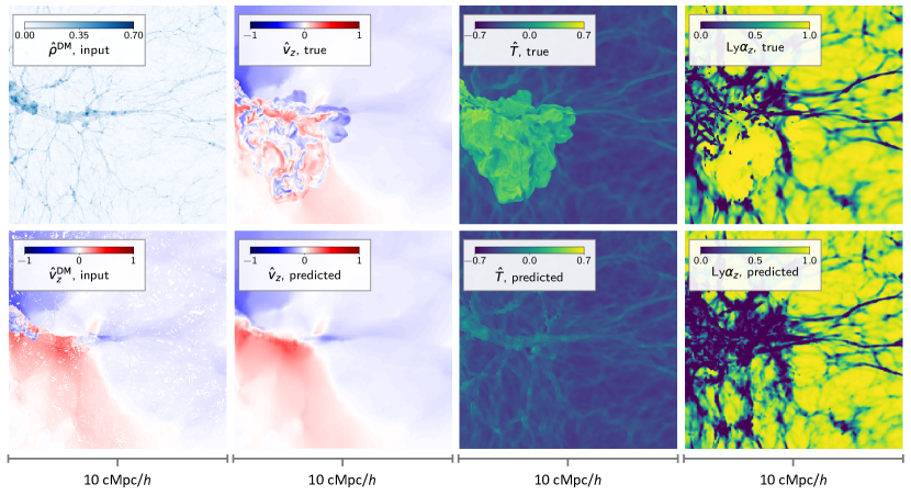
Figure 6: The widespread ($\sim 5$ cMpc) shocked region in the test simulation our model fails to capture. The left column shows some of the input dark matter fields, which indicate a dense cluster but do not otherwise contain information about the exact location and shape of a shock front. The middle panels show the baryon velocity and temperature fields at the same location, and reveal that the model has failed to capture the shock features. At far right, we show the Ly$\alpha$ slices corresponding to this shocked region.

Inspecting the test simulation more closely, we find a rare widespread shocked region of size $\sim 5$ cMpc, a significant fraction of the length of the entire box. In Figure 6 we show slices of this region for the true fields and our model’s reconstructions. It is clear that the model does not reproduce the shock structure, instead painting in a fairly smooth rendering of the filament structures in the area. Given that the model is trained on randomly-cropped sub-volumes of size 2.5 cMpc, it is unreasonable to expect coherent shock structures as large as this to be well-represented. Furthermore, as such structures form $O(1)$ times per 20 Mpc/$h$ box, they are exceedingly rare in the training data. In fact, there is no shocked region as large as this in the training simulation, hence the clear difference between the temperature PDFs in the train and test simulations.

5 Conclusion

In this work we have presented a convolutional neural network approach to map from collisionless n-body simulations to fully hydrodynamical simulations, reconstructing the baryon density, temperature and velocity fields. We find this mapping can match the statistical properties of the true hydrodynamical simulations across a wide range of scales. When computing an observable quantity, Ly$\alpha$ flux, from our model output, we can outperform existing semi-analytical methods across all scales and match the true simulated power-spectra within $\sim 5\%$ up to $k\sim 10$ $h$/Mpc.

The range of scales accurately mapped with this method is well beyond the resolution of next generation observations (Walther et al., 2021). This method provides an alternative to running costly hydrodynamical simulations for mock catalog generation and the construction of Ly$\alpha$ power-spectra emulators. The network can conveniently be trained on small simulated boxes at a given point in cosmological and astrophysical parameter space, then applied to a large dark matter only box at inference time. Thus, as the size of the inference box grows, this approach enables increasingly impressive reductions in computational cost.

Beyond Ly$\alpha$ forest statistics, there are some notable limitations to this method. Processes not well described by the dark matter distribution are difficult to predict, particularly the high temperature gas shocks seen in Figure 6. While these regions have limited effect on summary statistics used for Ly$\alpha$ cosmological analysis, they are of significant astrophysical interest as they are associated with the physics of the Warm Hot Intergalactic Medium (WHIM) (Cen & Ostriker, 1999; Pfrommer et al., 2006; Vazza et al., 2019). Considering our neural network design, the predictions in Figure 6 are not entirely unreasonable given the input dark matter fields from the n-body simulation (visualized in the far left panels). These inputs contain a dense cluster towards the edge, but do not have obvious indicators of the scale or detailed shape of the shock front. Thus, passing these inputs to a deterministic model such as ours yields a more conservative prediction, as the model does not have the expressive capacity to represent the many possible shapes of shocked gas. We thus propose that a variational model producing multi-modal outputs would best resolve shocks like the one shown in Figure 6. Such a model would synthesize multiple realizations of the hydrodynamic variables via some latent variable, conditioned on the input n-body fields. We explore this challenge in Horowitz et al. (2021), a companion work to this paper.

References

- Almgren et al. (2013) Almgren, A. S., Bell, J. B., Lijewski, M. J., Lukić, Z., & Van Andel, E. 2013, ApJ, 765, 39, doi: 10.1088/0004-637X/765/1/39
- Boera et al. (2019) Boera, E., Becker, G. D., Bolton, J. S., & Nasir, F. 2019, ApJ, 872, 101, doi: 10.3847/1538-4357/aafee4
- Cen & Ostriker (1999) Cen, R., & Ostriker, J. P. 1999, ApJ, 514, 1, doi: 10.1086/306949
- Chabanier et al. (2020) Chabanier, S., Bournaud, F., Dubois, Y., et al. 2020, MNRAS, 495, 1825, doi: 10.1093/mnras/staa1242
- Coc et al. (2013) Coc, A., Uzan, J.-P., & Vangioni, E. 2013, arXiv e-prints, arXiv:1307.6955. https://arxiv.org/abs/1307.6955
- Croft et al. (1999) Croft, R. A. C., Weinberg, D. H., Pettini, M., Hernquist, L., & Katz, N. 1999, ApJ, 520, 1, doi: 10.1086/307438
- Desjacques et al. (2006) Desjacques, V., Haehnelt, M. G., & Nusser, A. 2006, MNRAS, 367, L74, doi: 10.1111/j.1745-3933.2006.00143.x
- Friesen et al. (2016) Friesen, B., Almgren, A., Lukić, Z., et al. 2016, Computational Astrophysics and Cosmology, 3, 4, doi: 10.1186/s40668-016-0017-2
- Gnedin & Hui (1996) Gnedin, N. Y., & Hui, L. 1996, ApJ, 472, L73, doi: 10.1086/310366
- Gnedin & Hui (1998) —. 1998, MNRAS, 296, 44, doi: 10.1046/j.1365-8711.1998.01249.x
- Goodfellow et al. (2014) Goodfellow, I. J., Pouget-Abadie, J., Mirza, M., et al. 2014, arXiv e-prints, arXiv:1406.2661. https://arxiv.org/abs/1406.2661
- Gunn & Peterson (1965) Gunn, J. E., & Peterson, B. A. 1965, ApJ, 142, 1633, doi: 10.1086/148444
- Horowitz et al. (2019) Horowitz, B., Lee, K.-G., White, M., Krolewski, A., & Ata, M. 2019, ApJ, 887, 61, doi: 10.3847/1538-4357/ab4d4c
- Horowitz et al. (2020) Horowitz, B., Zhang, B., Lee, K.-G., & Kooistra, R. 2020, arXiv e-prints, arXiv:2007.15994. https://arxiv.org/abs/2007.15994
- Hui & Gnedin (1997) Hui, L., & Gnedin, N. Y. 1997, MNRAS, 292, 27, doi: 10.1093/mnras/292.1.27
- Iršič et al. (2017) Iršič, V., Viel, M., Haehnelt, M. G., et al. 2017, Phys. Rev. D, 96, 023522, doi: 10.1103/PhysRevD.96.023522
- Isola et al. (2016) Isola, P., Zhu, J.-Y., Zhou, T., & Efros, A. A. 2016, arXiv e-prints, arXiv:1611.07004. https://arxiv.org/abs/1611.07004
- Kollmeier et al. (2006) Kollmeier, J. A., Miralda-Escudé, J., Cen, R., & Ostriker, J. P. 2006, ApJ, 638, 52, doi: 10.1086/498104
- Lukić et al. (2015) Lukić, Z., Stark, C. W., Nugent, P., et al. 2015, MNRAS, 446, 3697, doi: 10.1093/mnras/stu2377
- Maas et al. (2013) Maas, A. L., Hannun, A. Y., & Ng, A. Y. 2013, in Proc. icml, Vol. 30, 3
- McQuinn (2016) McQuinn, M. 2016, Annual Review of Astronomy and Astrophysics, 54, 313, doi: 10.1146/annurev-astro-082214-122355
- Nair & Hinton (2010) Nair, V., & Hinton, G. E. 2010, in Proceedings of the 27th international conference on machine learning (ICML-10), 807–814
- Oñorbe et al. (2019) Oñorbe, J., Davies, F. B., Lukić, et al. 2019, MNRAS, 486, 4075, doi: 10.1093/mnras/stz984
- Palanque-Delabrouille et al. (2020) Palanque-Delabrouille, N., Yèche, C., Schöneberg, N., et al. 2020, J. Cosmology Astropart. Phys, 2020, 038, doi: 10.1088/1475-7516/2020/04/038
- Pedersen et al. (2020) Pedersen, C., Font-Ribera, A., Rogers, K. K., et al. 2020, arXiv e-prints, arXiv:2011.15127. https://arxiv.org/abs/2011.15127
- Peirani et al. (2014) Peirani, S., Weinberg, D. H., Colombi, S., et al. 2014, ApJ, 784, 11, doi: 10.1088/0004-637X/784/1/11
- Petitjean et al. (1995) Petitjean, P., Mueket, J. P., & Kates, R. E. 1995, A&A, 295, L9. https://arxiv.org/abs/astro-ph/9502100
- Pfrommer et al. (2006) Pfrommer, C., Springel, V., Enßlin, T. A., & Jubelgas, M. 2006, MNRAS, 367, 113, doi: 10.1111/j.1365-2966.2005.09953.x
- Porqueres et al. (2019) Porqueres, N., Jasche, J., Lavaux, G., & Enßlin, T. 2019, A&A, 630, A151, doi: 10.1051/0004-6361/201936245
- Rauch et al. (1997) Rauch, M., Miralda-Escudé, J., Sargent, W. L. W., et al. 1997, ApJ, 489, 7, doi: 10.1086/304765
- Rogers et al. (2018) Rogers, K. K., Bird, S., Peiris, H. V., et al. 2018, MNRAS, 474, 3032, doi: 10.1093/mnras/stx2942
- Rogers & Peiris (2020) Rogers, K. K., & Peiris, H. V. 2020, arXiv e-prints, arXiv:2007.12705. https://arxiv.org/abs/2007.12705
- Ronneberger et al. (2015) Ronneberger, O., Fischer, P., & Brox, T. 2015, in International Conference on Medical image computing and computer-assisted intervention, Springer, 234–241
- Seljak (2012) Seljak, U. 2012, J. Cosmology Astropart. Phys, 2012, 004, doi: 10.1088/1475-7516/2012/03/004
- Sorini et al. (2016) Sorini, D., Oñorbe, J., Lukić, Z., & Hennawi, J. F. 2016, ApJ, 827, 97, doi: 10.3847/0004-637X/827/2/97
- Thiele et al. (2020) Thiele, L., Villaescusa-Navarro, F., Spergel, D. N., Nelson, D., & Pillepich, A. 2020, ApJ, 902, 129, doi: 10.3847/1538-4357/abb80f
- Tröster et al. (2019) Tröster, T., Ferguson, C., Harnois-Déraps, J., & McCarthy, I. G. 2019, MNRAS, 487, L24, doi: 10.1093/mnrasl/slz075
- Upton Sanderbeck & Bird (2020) Upton Sanderbeck, P., & Bird, S. 2020, MNRAS, 496, 4372, doi: 10.1093/mnras/staa1850
- Vazza et al. (2019) Vazza, F., Ettori, S., Roncarelli, M., et al. 2019, A&A, 627, A5, doi: 10.1051/0004-6361/201935439
- Walther et al. (2021) Walther, M., Armengaud, E., Ravoux, C., et al. 2021, J. Cosmology Astropart. Phys, 2021, 059, doi: 10.1088/1475-7516/2021/04/059
- Walther et al. (2019) Walther, M., Oñorbe, J., Hennawi, J. F., & Lukić, Z. 2019, ApJ, 872, 13, doi: 10.3847/1538-4357/aafad1
- Zamudio-Fernandez et al. (2019) Zamudio-Fernandez, J., Okan, A., Villaescusa-Navarro, F., et al. 2019, arXiv e-prints, arXiv:1904.12846. https://arxiv.org/abs/1904.12846