Extreme Multi-label Learning for
Semantic Matching in Product Search

Abstract.

We consider the problem of semantic matching in product search: given a customer query, retrieve all semantically related products from a huge catalog of size $100$ million, or more. Because of large catalog spaces and real-time latency constraints, semantic matching algorithms not only desire high recall but also need to have low latency. Conventional lexical matching approaches (e.g., Okapi-BM25) exploit inverted indices to achieve fast inference time, but fail to capture behavioral signals between queries and products. In contrast, embedding-based models learn semantic representations from customer behavior data, but the performance is often limited by shallow neural encoders due to latency constraints. Semantic product search can be viewed as an eXtreme Multi-label Classification (XMC) problem, where customer queries are input instances and products are output labels. In this paper, we aim to improve semantic product search by using tree-based XMC models where inference time complexity is logarithmic in the number of products. We consider hierarchical linear models with n-gram features for fast real-time inference. Quantitatively, our method maintains a low latency of $1.25$ milliseconds per query and achieves a $65\%$ improvement of Recall@100 ($60.9\%$ v.s. $36.8\%$) over a competing embedding-based DSSM model. Our model is robust to weight pruning with varying thresholds, which can flexibly meet different system requirements for online deployments. Qualitatively, our method can retrieve products that are complementary to existing product search system and add diversity to the match set.

1. Introduction

In general, product search consists of two building blocks: the matching stage, followed by the ranking stage. When a customer issues a query, the query is passed to several matching algorithms to retrieve relevant products, resulting in a match set. The match set passes through stages of ranking, where top results from the previous stage are re-ranked before the most relevant items are displayed to customers. Figure 1 outlines a product search system.

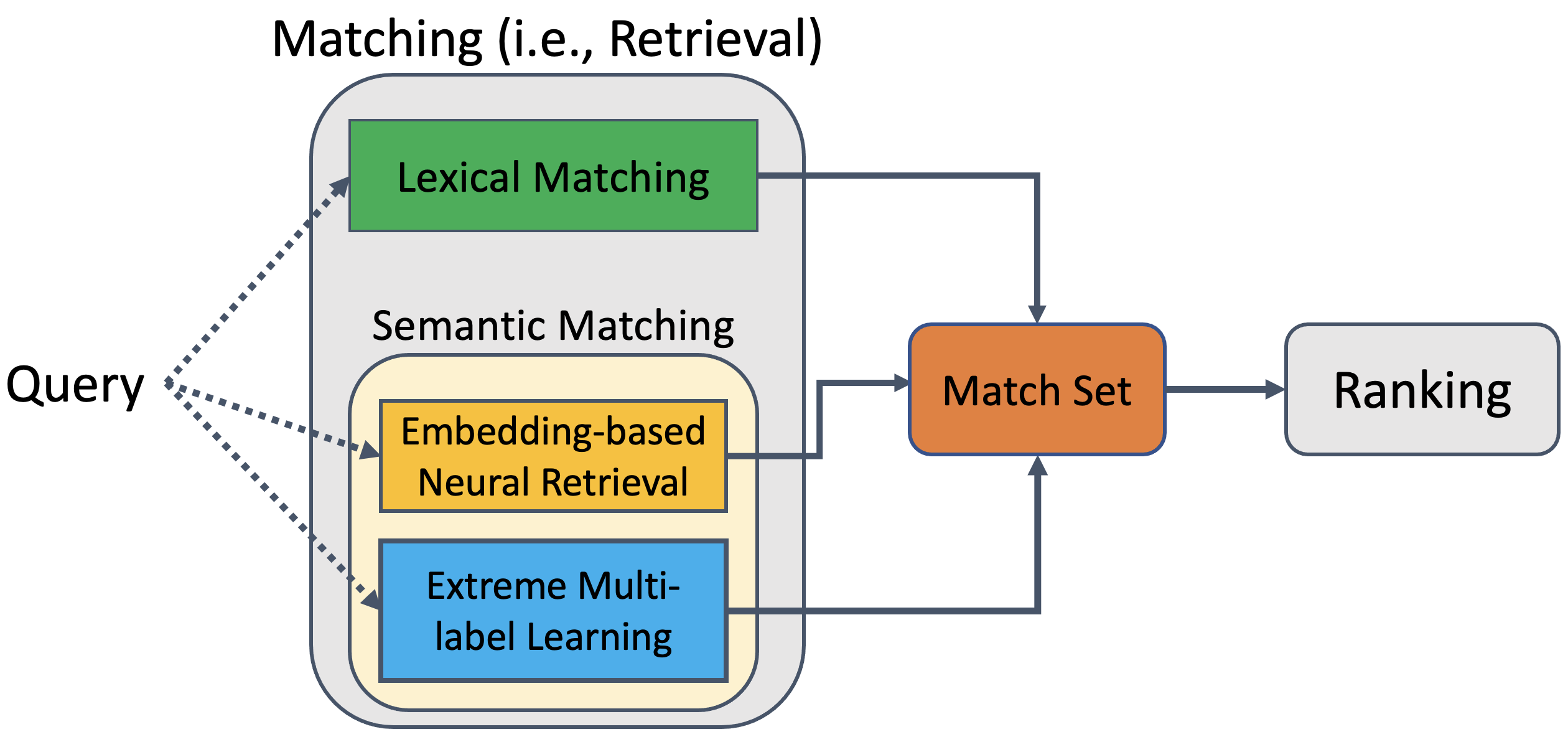
Figure 1. System architecture for augmenting match set with extreme multi-label learning models.

The matching (i.e., retrieval) phase is critical. Ideally, the match set should have a high recall (Manning et al., 2008), containing as many relevant and diverse products that match the customer intent as possible; otherwise, many relevant products won’t be considered in the final ranking phase. On the other hand, the matching algorithm should be highly efficient to meet real-time inference constraints: retrieving a small subset of relevant products in time sublinear to enormous catalog spaces, whose size is as large as 100 million or more.

Matching algorithms can be put into two categories. The first type is lexical matching approaches that score a query-product pair by a weighted sum of overlapping keywords among the pair. One representative example is Okapi-BM25 (Robertson and Walker, 1994; Robertson et al., 2009), which remains state-of-the-art for decades and is still widely used in many retrieval tasks such as open-domain question answering (Lee et al., 2019; Chang et al., 2020a) and passage/document retrieval (Gao et al., 2020; Boytsov and Nyberg, 2020). While the inference of Okapi-BM25 can be done efficiently using an inverted index (Zobel and Moffat, 2006), these index-based lexical matching approaches cannot capture semantic and customer behavior signals (e.g., clicks, impressions, or purchases) tailored from the product search system and are fragile to morphological variants or spelling errors.

The second option is embedding-based neural models that learn semantic representations of queries and products based on the customer behavior signals. The similarity is measured by inner products or cosine distances between the query and product embeddings. To infer in real-time the match set of a novel query, embedding-based neural models need to first vectorize the query tokens into the query embedding, and then find its nearest neighbor products in the embedding space. Finding nearest neighbors can be done efficiently via approximate nearest neighbor search (ANN) methods (e.g., HNSW (Malkov and Yashunin, 2020) or ScaNN (Guo et al., 2020)). Vectorizing query tokens into an embedding, nevertheless, is often the inference bottleneck, that depends on the complexity of neural network architectures.

Using BERT-based encoders (Devlin et al., 2019) for query embeddings is less practical because of the large latency in vectorizing queries. Specifically, consider retrieving the match set of a query from the output space of $100$ millions of products on a CPU machine. In Table 1, we compare the latency of a BERT-based encoder ($12$ layers deep Transformer) with a shallow DSSM (Nigam et al., 2019) encoder ($2$ layers MLP). The inference latency of a BERT-based encoder is $50$ milliseconds per query (ms$/$q) in total, where vectorization and ANN search needs $88\%$ and $12\%$ of the time, respectively. On the other hand, the latency of DSSM encoder is $3.13$ ms$/$q in total, where vectorization only takes $33\%$ of the time.

Vectorizer	latency (ms$/$q)	ANN	latency (ms$/$q)
DSSM (Nigam et al., 2019)	1.00	HNSW (Malkov and Yashunin, 2020)	2.13
BERT-based (Devlin et al., 2019)	44.00	HNSW (Malkov and Yashunin, 2020)	$\approx 6.39$

Table 1. Comparing inference latency of BERT-based encoder with DSSM encoder on a CPU machine, with single-batch, single-thread settings. The latency of BERT-based encoder is taken from HuggingFace Transformers (Wolf et al., 2020, [n.d.]). BERT’s ANN time is estimated by linear extrapolation on the dimensionality $d$, where BERT has $d=768$ and DSSM has $d=256$.

Because of real-time inference constraints, industrial product search engines do not have the luxury to leverage state-of-the-art deep Transformer encoders in embedding-based neural methods, whereas shallow MLP encoders result in limited performance.

In this paper, we take another route to tackle semantic matching by formulating it as an eXtreme Multi-label Classification (XMC) problem, where the goal is tagging an input instance (i.e., query) with most relevant output labels (i.e., products). XMC approaches have received great attention recently in both the academic and industrial community. For instance, the deep learning XMC model X-Transformer (Chang et al., 2020b; Yu et al., 2020) achieves state-of-the-art performance on public academic benchmarks (Bhatia et al., 2016). Partition-based methods such as Parabel (Prabhu et al., 2018) and XReg (Prabhu et al., 2020), as another example, finds successful applications to dynamic search advertising in Bing. In particular, tree-based partitioning XMC models are a staple of modern search engines and recommender systems due to their inference time being sub-linear (i.e., logarithmic) to the enormous output space (e.g., $100$ million or more).

In this paper, we aim to answer the following research question: Can we develop an effective tree-based XMC approach for semantic matching in product search? Our goal is not to replace lexical-based matching methods (e.g., Okapi-BM25). Instead, we aim to complement/augment the match set with more diverse candidates from the proposed tree-based XMC approaches; hence the final stage ranker can produce a good and diverse set of products in response to search queries.

We make the following contributions in this paper.

• We apply the leading tree-based XR-Linear (PECOS) model (Yu et al., 2020) to semantic matching. To our knowledge, we are the first to successfully apply tree-based XMC methods to an industrial scale product search system.

• We explore various $n$-gram TF-IDF features for XR-Linear as vectorizing queries into sparse TF-IDF features is highly efficient for real-time inference.

• We study weight pruning of the XR-Linear model and demonstrate its robustness to different disk-space requirements.

• We present the trade-off between recall rates and real-time latency. Specifically, for beam size $b=15$, XR-Linear achieves Recall$@100$ of $60.9\%$ with a latency of $1.25$ ms$/$q; for beam size $b=50$, XR-Linear achieves Recall$@100$ of $65.7\%$ with a latency of $3.48$ ms$/$q. In contrast, DSSM only has Recall$@100$ of $36.2\%$ with a latency of $3.13$ ms$/$q.

The implementation of XR-Linear (PECOS) is publicly available at https://github.com/amzn/pecos.

2. Related Work

2.1. Semantic Product Search Systems

Two-tower models (a.k.a., dual encoders, Siamese networks) are arguably one of the most popular embedding-based neural models used in passage or document retrieval (Nguyen et al., 2016; Xiong et al., 2021), dialogue systems (Mazaré et al., 2018; Henderson et al., 2019), open-domain question answering (Lee et al., 2019; Guu et al., 2020; Karpukhin et al., 2020), and recommender systems (Covington et al., 2016; Yi et al., 2019; Yang et al., 2020). It is not surprising that two-tower models with ResNet (He et al., 2016) encoder and deep Transformer encoders (Vaswani et al., 2017) achieve state-of-the-art in most computer vision (Kuznetsova et al., 2020) and textual-domain retrieval benchmarks (Craswell et al., 2020), respectively. The more complex the encoder architecture is, nevertheless, the less applicable the deep two-tower models are for industrial product search systems: very few of them can meet the low real-time latency constraint (e.g., 5 ms/q) due to the vectorization bottleneck of query tokens.

One of the exceptions is Deep Semantic Search Model (DSSM) (Nigam et al., 2019), a variant of two-tower retrieval models with shallow multi-layer perceptron (MLP) layers. DSSM is tailored for industrial-scale semantic product search, and was A/B tested online on Amazon Search Engine (Nigam et al., 2019). Another example is two-tower recommender models for Youtube (Covington et al., 2016) and Google Play (Yang et al., 2020), where they also embrace shallow MLP encoders for fast vectorization of novel queries to meet online latency constraints. Finally, (Song et al., 2020) leverages distributed GPU training and KNN softmax, scaling two-tower models for the Alibaba Retail Product Dataset with $100$ million products.

2.2. eXtreme Multi-label Classification (XMC)

To overcome computational issues, most existing XMC algorithms with textual inputs use sparse TF-IDF features and leverage different partitioning techniques on the label space to reduce complexity.

Sparse linear models

Linear one-versus-rest (OVR) methods such as DiSMEC (Babbar and Schölkopf, 2017), ProXML (Babbar and Schölkopf, 2019), PPD-Sparse (Yen et al., 2016; Yen et al., 2017) explore parallelism to speed up the algorithm and reduce the model size by truncating model weights to encourage sparsity. Linear OVR classifiers are also building blocks for many other XMC approaches, such as Parabel (Prabhu et al., 2018), SLICE (Jain et al., 2019), XR-Linear (PECOS) (Yu et al., 2020), to name just a few. However, naive OVR methods are not applicable to semantic product search because their inference time complexity is still linear in the output space.

Partition-based methods

The efficiency and scalability of sparse linear models can be further improved by incorporating different partitioning techniques on the label spaces. For instance, Parabel (Prabhu et al., 2018) partitions the labels through a balanced 2-means label tree using label features constructed from the instances. Other approaches attempt to improve on Parabel, for instance, eXtremeText (Wydmuch et al., 2018), Bonsai (Khandagale et al., 2020), NAPKINXC (Jasinska-Kobus et al., 2020), XReg (Prabhu et al., 2020), and  PECOS (Yu et al., 2020). In particular, the PECOS framework (Yu et al., 2020) allows different indexing and matching methods for XMC problems, resulting in two realizations, XR-Linear and X-Transformer. Also note that tree-based methods with neural encoders such as AttentionXML (You et al., 2019), X-Transformer (PECOS) (Chang et al., 2020b; Yu et al., 2020), and LightXML (Jiang et al., 2021), are mostly the state-of-the-art results on XMC benchmarks, at the cost of longer training time and expensive inference. To sum up, tree-based sparse linear methods are more suitable for the industrial-scale semantic matching problems due to their sub-linear inference time and fast vectorization of the query tokens.

Graph-based methods

SLICE (Jain et al., 2019) and AnnexML (Tagami, 2017) building an approximate nearest neighbor (ANN) graph to index the large output space. For a given instance, the relevant labels can be found quickly via ANN search. SLICE then trains linear OVR classifiers with negative samples induced from ANN. While the inference time complexity of advanced ANN algorithms (e.g., HNSW (Malkov and Yashunin, 2020) or ScaNN (Guo et al., 2020)) is sub-linear, ANN methods typically work better on low-dimensional dense embeddings. Therefore, the inference latency of SLICE and AnnexML still hinges on the vectorization time of pre-trained embeddings.

3. XR-Linear (PECOS): a tree-based XMC method for semantic matching

Overview

Tree-based XMC models for semantic matching can be characterized as follows: given a vectorized query $\mathbf{x}\in\mathbb{R}^{d}$ and a set of labels (i.e., products) $\mathcal{Y}=\{1,\ldots,\ell,\ldots,L\}$, produce a tree-based model that retrieves top $k$ most relevant products in $\mathcal{Y}$. The model parameters are estimated from the training dataset $\{(\mathbf{x}_{i},\mathbf{y}_{i}):i=1,\ldots,n\}$ where $\mathbf{y}_{i}\in\{0,1\}^{L}$ denotes the relevant labels for this query from the output label space $\mathcal{Y}$.

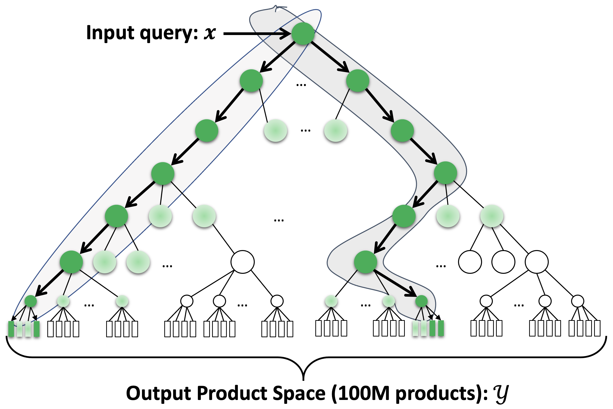
Figure 2. Illustration of inference of XR-Linear (PECOS) (Yu et al., 2020) using beam search with beam width $b=2$ to retrieve $4$ relevant products for the given input query $\mathbf{x}$.

There are many tree-based linear methods  (Prabhu et al., 2018; Wydmuch et al., 2018; Khandagale et al., 2020; Jasinska-Kobus et al., 2020; Prabhu et al., 2020; Yu et al., 2020), and we consider the XR-Linear model within PECOS (Yu et al., 2020) in this paper, due to its flexibility and scalability to large output spaces. The XR-Linear model partitions the enormous label space $\mathcal{Y}$ with hierarchical clustering to form a hierarchical label tree. The $j$th label cluster at depth $t$ is denoted by $\mathcal{Y}^{(t)}_{j}$. The leaves of the tree are the individual labels (i.e., products) of $\mathcal{Y}$. See Figure 2 for an illustration of the tree structure and inference with beam search.

Each layer of the XR-Linear model has a linear OVR classifier that scores the relevance of a cluster $\mathcal{Y}^{(t)}_{j}$ to a query $\mathbf{x}$. Specifically, the unconditional relevance score of a cluster $\mathcal{Y}^{(t)}_{j}$ is

(1) $$f(\mathbf{x},\mathcal{Y}^{(t)}_{j})=\sigma(\mathbf{x}^{\top}\mathbf{w}^{(t)}_{j}),$$

where $\sigma$ is an activation function and $\mathbf{w}^{(t)}_{j}\in\mathbb{R}^{d}$ are model parameters of the $j$-th node at $t$-th layer.

Practically, the weight vectors $\mathbf{w}^{(t)}_{j}$ for each layer $t$ are stored in a $d\times K_{t}$ weight matrix

(2) $$\mathbf{W}^{(t)}=\left[\begin{array}[]{cccc}\mathbf{w}^{(t)}_{1}&\mathbf{w}^{(t)}_{2}&...&\mathbf{w}^{(t)}_{K_{t}}\end{array}\right]\,,$$

where $K_{t}$ denotes the number of clusters at layer $t$, such that $K_{D}=L$ and $K_{0}=1$. In addition, the tree topology at layer $t$ is represented by a cluster indicator matrix $\mathbf{C}^{(t)}\in\{0,1\}^{K_{t+1}\times K_{t}}$. Next, we discuss how to construct the cluster indicator matrix $\mathbf{C}^{(t)}$ and learn the model weight matrix $\mathbf{W}^{(t)}$.

3.1. Hierarchical Label Tree

Tree Construction

Given semantic label representations $\{\mathbf{z}_{\ell}:\mathcal{Y}\}$, the XR-Linear model constructs a hierarchical label tree via $B$ array partitioning (i.e., clustering) in a top-down fashion, where the number of clusters at layer $t=1,\ldots,D$ are

(3) $$K_{D}=L,K_{D-1}=B^{D-1},\ldots,K_{1}=B^{1}.$$

Starting from the node $k$ of layer $t-1$ is a cluster $\mathcal{Y}^{(t)}_{k}$ containing labels assigned to this cluster. For example, $\mathcal{Y}^{(0)}_{1}=\mathcal{Y}$ is the root node clustering including all the labels $\{\ell:1,\ldots,L\}$. To proceed from layer $t-1$ to layer $t$, we perform Spherical $B$-Means (Dhillon and Modha, 2001) clustering to partition $\mathcal{Y}^{(t-1)}_{k}$ into $B$ clusters to form its $B$ child nodes $\{\mathcal{Y}^{(t)}_{B(k-1)+j}:j=1,\ldots,B\}$. Applying this for all parent nodes $k=1,\ldots,B^{t-1}$ at layer $t-1$, the cluster indicator matrix $\mathbf{C}^{(t)}\in\{0,1\}^{K_{t}\times K_{t-1}}$ at layer $t$ is represented by

(4) $$\Big{(}\mathbf{C}^{(t)}\Big{)}_{j,k}=\begin{cases}1,&\text{ if }\mathcal{Y}^{(t)}_{j}\text{ is a child of }\mathcal{Y}^{(t-1)}_{k},\\ 0,&\text{ otherwise}.\end{cases}$$

An illustration with $B=2$ is given in Figure 3.

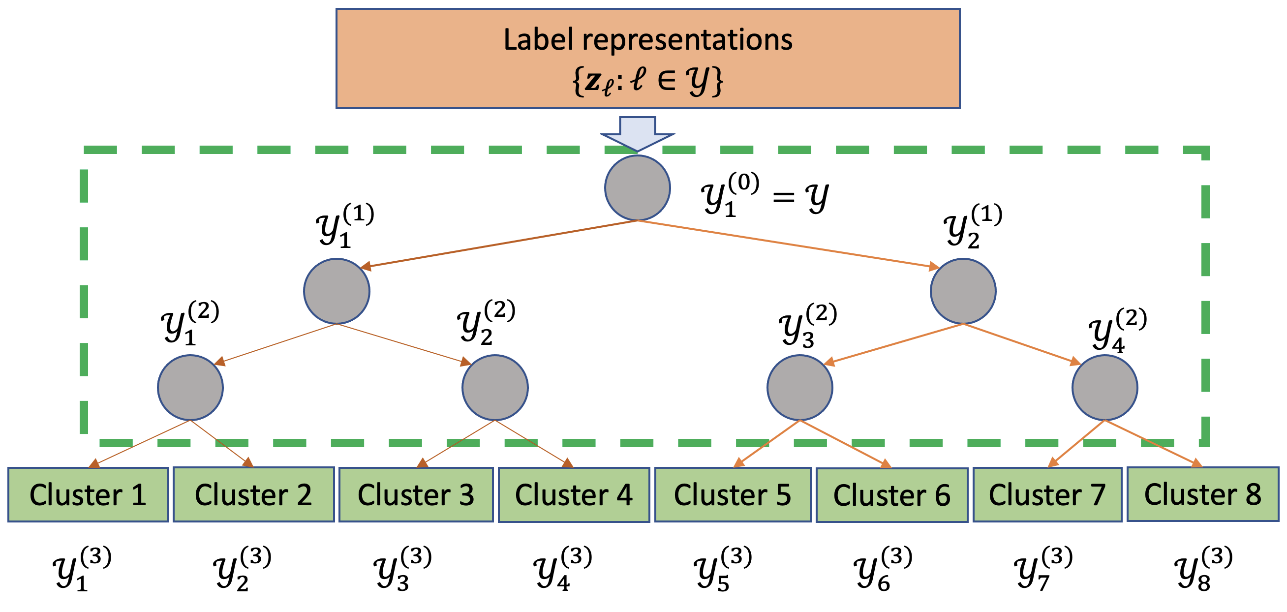
Figure 3. An illustration of hierarchical label clustering (Yu et al., 2020) with recursive $B$-ary partitions with $B=2$.

Label Representations

For semantic matching problem, we present two ways to construct label embeddings, depending on the quality of product information (i.e., titles and descriptions). If product information such as titles and descriptions are noisy or missing, each label is represented by aggregating query feature vectors from positive instances (namely, PIFA):

(5) $$\mathbf{z}_{\ell}^{{\sf PIFA}}=\frac{\mathbf{v}_{\ell}}{\|\mathbf{v}_{\ell}\|},\text{ where }\mathbf{v}_{\ell}=\sum_{i=1}^{n}\mathbf{Y}_{i\ell}\mathbf{x}_{i},\quad\ell\in\mathcal{Y}.$$

Otherwise, labels with rich textual information can be represented by featurization (e.g., $n$-gram TF-IDF or some pre-trained neural embeddings) of its titles and descriptions.

3.2. Sparse Linear Matcher

Given the query feature matrix $\mathbf{X}\in\mathbb{R}^{n\times d}$, the label matrix $\mathbf{Y}\in\{0,1\}^{n\times L}$, and cluster indicator matrices $\{\mathbf{C}^{(t)}\in\{0,1\}^{K_{t}\times K_{t-1}}:K_{0}=1,K_{D}=L,t=1,\ldots,D\}$, we are ready to learn the model parameters $\mathbf{W}^{(t)}$ for layer $t=1,\ldots,D$ in a top-down fashion. For example, at the bottom layer $t=D$, it corresponds to the original XMC problem on the given training data $\{\mathbf{X},\mathbf{Y}^{D}=\mathbf{Y}\}$. For layer $t=D-1$, we construct the XMC problem with the induced dataset $\{\mathbf{X},\mathbf{Y}^{D-1}=\text{binarize}(\mathbf{Y}^{D}\mathbf{C}^{(D)})\}$. Similar recursion is applied to all other intermediate layers.

Learning OVR Classifiers

At layer $t$ with the corresponding XMC dataset $\{\mathbf{X},\mathbf{Y}^{t}\}$, the XR-Linear model considers point-wise loss to learn the parameter matrix $\mathbf{W}^{(t)}\in\mathbb{R}^{d\times K_{t}}$ independently for each column $\ell$, $1\leq\ell\leq K_{t}$. Column $\ell$ of $\mathbf{W}^{(t)}$ is found by solving a binary classification sub-problem:

(6) $$\mathbf{w}^{(t)}_{\ell}=\arg\min_{\mathbf{w}}\sum_{i:\mathcal{M}^{(t)}_{i,\mathbf{c}_{\ell}}\neq 0}\mathcal{L}(\mathbf{Y}_{i\ell}^{t},\mathbf{w}^{\top}\mathbf{x}_{i})+\frac{\lambda}{2}\|\mathbf{w}\|_{2}^{2},\quad\ell=1,\ldots,K_{t},$$

where $\lambda$ is the regularization coefficient, $\mathcal{L}(\cdot,\cdot)$ is the point-wise loss function (e.g., squared hinge loss), $\mathcal{M}^{(t)}\in\{0,1\}^{n\times K_{t-1}}$ is a negative sampling matrix at layer $t$, and $\mathbf{c}_{\ell}=\mathbf{c}_{\ell}^{t}\in\{1,\ldots,K_{t-1}\}$ is the cluster index of the $\ell$-th label (cluster) at the $t$-th layer. Crucially, the negative sampling matrix $\mathcal{M}^{(t)}$ not only finds hard negative instances (queries) for stronger learning signals, but also significantly reduces the size of the active instance set for faster convergence.

In practice, we solve the binary classification sub-problem  (6) via a state-of-the-art efficient solver LIBLINEAR (Fan et al., 2008). Furthermore, $K_{t}$ independent sub-problems at layer $t$ can be computed in an embarrassingly parallel manner to fully utilize the multi-core CPU design in modern hardware.

3.3. Inference

Weight Pruning

The XR-Linear model is composed of $D$ OVR linear classifiers $f^{(t)}(\mathbf{x},\ell)$ parametrized by matrices $\mathbf{W}^{(t)}\in\mathbb{R}^{d\times K_{t}}$, $1\leq t\leq D$ Naively storing the dense parameter matrices is not feasible. To overcome a prohibitive model size, we apply entry-wise weight pruning to sparsify $\mathbf{W}^{(t)}$ (Babbar and Schölkopf, 2017; Prabhu et al., 2018). Specifically, after solving $\mathbf{w}^{(t)}_{\ell}$ for each binary classification sub-problem, we perform a hard thresholding operation to truncate parameters with magnitude smaller than a pre-specified value $\epsilon\geq 0$ to zero:

(7) $$\Big{(}\mathbf{W}^{(t)}\Big{)}_{ij}=\begin{cases}\mathbf{W}^{(t)}_{ij},&\text{ if }|\mathbf{W}^{(t)}_{ij}|>\epsilon,\\ 0,&\text{ otherwise}.\end{cases}$$

We set the pruning threshold $\epsilon$ such that the parameter matrices can be stored in the main memory for real-time inference.

Beam Search

The relevance score of a query-cluster pair $(\mathbf{x},\tilde{\mathcal{Y}})$ is defined to be the aggregation of all ancestor nodes in the tree:

(8) $$f(\mathbf{x},\tilde{\mathcal{Y}})=\prod_{\mathbf{w}\in\mathcal{A}(\tilde{\mathcal{Y}})}\sigma\left(\mathbf{w}\cdot\mathbf{x}\right)\,,$$

where $\mathcal{A}(\tilde{\mathcal{Y}})=\{\mathbf{w}^{(t)}_{i}\mid\tilde{\mathcal{Y}}\subset\mathcal{Y}^{(t)}_{i},t\neq 0\}$ denotes the weight vectors of all ancestors of $\tilde{\mathcal{Y}}$ in the tree, including $\tilde{\mathcal{Y}}$ and disregarding the root. Naturally, this definition extends all the way to the individual labels $\ell\in\mathcal{Y}$ at the bottom of the tree.

In practice, exact inference is typically intractable, as it requires searching the entire label tree. To circumvent this issue, XR-Linear use a greedy beam search of the tree as an approximation. For a query $\mathbf{x}$, this approach discards any clusters at a given level that do not fall into the top $b$ most relevant clusters, where $b$ is the beam search width. The inference time complexity of XR-Linear with beam search (Yu et al., 2020) is

(9) $$\sum_{t=1}^{D}\mathcal{O}\Big{(}b\times\frac{K_{t}}{K_{t-1}}\times T_{f}\big{)}=\mathcal{O}\Big{(}D\times b\times\max\big{(}B,\frac{L}{B^{D-1}}\big{)}\times T_{f}\Big{)},$$

where $T_{f}$ is the time to compute relevance score $f^{(t)}(\mathbf{x},\ell)$. We see that if the tree depth $D=\mathcal{O}(\log_{B}L)$ and max leaf size $L/B^{D-1}$ is a small constant such as $100$, the overall inference time complexity for XR-Linear is

(10) $$\mathcal{O}(b\times T_{f}\times\log L),$$

which is logarithmic in the size of the original output space.

3.4. Tokenization and Featurization

To pre-process the input query or product title, we apply simple normalization (e.g., lower case, remove basic punctuations) and use white space to tokenize the query string into a sequence of smaller components such as words, phrases, or characters. We combine word unigrams, word bigrams, and character trigrams into a bag of $n$-grams feature, and construct sparse high-dimensional TF-IDF features as the vectorization of the query.

Word $n$-grams

The basic form of tokenization is a word unigram. For example, the word unigrams of ”artistic iphone 6s case” are [”artistic”, ”iphone”, ”6s”, ”case”]. However, word unigrams lose word ordering information, which leads us to use higher order $n$-grams, such as bigrams. For example, the word bigram of the same query becomes [”artistic#iphone”, ”iphone#6s”, ”6s#case”]. These $n$-grams capture phrase-level information which helps the model to better infer the customer intent for search.

Character Trigrams

The string is broken into a list of all three-character sequences, and we only consider the trigrams within word boundary. For example, the character trigrams of the query ”artistic iphone 6s case” are [”#ar”, ”art”, ”rti”, ”tis”, ”ist”, ”sti”, ”tic”, ”ic#”, ”#ip”, ”iph”, ”phi”, ”hon”, ”one”, ”#6s”, ”6s#”, ”#ca”, ”cas”, ”ase”, ”se#”]. Character trigrams are robust to typos (”iphone” and ”iphonr”) and can handle compound words (”amazontv” and ”firetvstick”) more naturally. Another advantage for product search is the ability to capture similarity of model parts and sizes.

4. Experimental Results

4.1. Data Preprocessing

We sample over $1$ billion positive query-product pairs as the data set, which covers over $240$ million queries and $100$ million products. A positive pair means aggregated counts of clicks or purchases are above a threshold. While each query-product pair may have a real-valued weight representing the aggregated counts, we do not currently leverage this information and simply treat the training signals as binary feedback. We split the train/test set by time horizon where we use $12$ months of search logs as the training set and the trailing $1$ month as the offline evaluation test set. Approximately 12% of products in the test set are unseen in the training set, which are also known as cold-start products.

For the XR-Linear model and Okapi-BM25, we consider white space tokenization for both query text and product title to vectorize the query feature and product features with $n$-gram TF-IDF. The training signals are extremely sparse, and the resulting query feature matrix has an average of $27.3$ non zero elements per query and the product feature matrix has an average of $142.1$ non zero element per product, with the dimensionality $d=4.2M$. For the DSSM model, both the query feature matrix and product feature matrix are dense low-dimensional (i.e., 256) embeddings, which are more suitable for HNSW inference.

Featurization

For the proposed XR-Linear method, we consider $n$-gram sparse TF-IDF features for the input queries and conduct $\ell_{2}$ normalization of each query vector. The vocabulary size is $4.2$ million, which is determined by the most frequent tokens of word and character level $n$-grams. In particular, there are $1$ million word unigrams, $3$ million word bigrams, and $200$ thousand character trigrams. Note that we consider characters within each word boundary when building the character level $n$-grams vocabulary. The motivation of using character trigrams is to better capture specific model types, certain brand names, and typos.

For out-of-vocabulary (OOV) tokens, we map those unseen tokens into a shared unique token id. It is possible to construct larger bins with hashing tricks  (Weinberger et al., 2009; Joulin et al., 2017; Nigam et al., 2019) that potentially handle the OOV tokens better. We leave the hashing tricks as future work.

4.2. Experimental Setup

Evaluation Protocol

We sample $100,000$ queries as the test set, which comprises $182,000$ query-product pairs with purchase counts being at least one. Given a query in the retrieval stage, semantic matching algorithms need to find the top $100$ relevant products from the catalog space consisting of $100$ million candidate products.

We measure the performance with recall metrics, which are widely-used in retrieval (Chang et al., 2020a; Xiong et al., 2021) and XMC tasks (Prabhu et al., 2018; Reddi et al., 2019; Jain et al., 2019). Specifically, for a predicted score vector $\hat{\mathbf{y}}\in\mathbb{R}^{L}$ and a ground truth label vector $\mathbf{y}\in\{0,1\}^{L}$, Recall$@k$ $(k=10,50,100)$ is defined as

$$\text{Recall}@k=\frac{\ell}{|\mathbf{y}|}\sum_{\ell\in\text{top}_{k}(\hat{\mathbf{y}})}\mathbf{y}_{\ell},$$

where $\text{top}_{k}(\hat{\mathbf{y}})$ denotes the labels with the largest $k$ predict values.

Comparing Methods and Hyper-parameters

We compare XR-Linear with two representative retrieval approaches and describe the hyper-parameter settings.

• XR-Linear: the proposed tree-based XMC model, where the implementation is from PECOS (Yu et al., 2020). We use PIFA to construct semantic product embeddings and build the label tree via hierarchical K-means, where the branching factor is $B=32$, the tree depth is $D=5$, and the maximum number of labels in each cluster is $L/B^{D-1}=100$. The negative sampling strategy is Teacher Forcing Negatives (TFN) (Yu et al., 2020), the transformation predictive function is $\mathcal{L}_{3}$ hinge, and default beam size is $b=10$. Unless otherwise specified, we follow the default hyper-parameter settings of PECOS.

• DSSM (Nigam et al., 2019): the leading neural embedding-based retrieval model in semantic product search applications. We take a saved checkpoint DSSM model from  (Nigam et al., 2019), and generate query and product embeddings on our dataset for evaluation. For fast real-time inference, we use the state-of-the-art approximate nearest neighbor (ANN) search algorithm HNSW (Malkov and Yashunin, 2020) to retrieve relevant products efficiently. Specifically, we use the implementation of NMSLIB (Boytsov and Naidan, 2013). Regarding the hyper-parameter of HNSW, we set $M_{0}=32$, $efC=300$, and vary the beam search width $efS=\{10,50,100,250,500\}$ to see trade-off between inference latency and retrieval quality.

• Okapi-BM25 (Robertson et al., 2009): the lexical matching baseline widely-used in retrieval tasks. We use the implementation of (Trotman et al., 2014) where hyper-parameters are set to $k_{1}=0.5$ and $b=0.45$.

Computing Environments

We run XR-Linear and Okapi-BM25 on a x1.32xlarge AWS instance ($128$ CPUs and $1952$ GB RAM). For the embedding-based model DSSM, the query and product embeddings are generated from a pre-trained DSSM model (Nigam et al., 2019) on a p3.16xlarge AWS instance (8 Nvidia V100 GPUs and $128$ GB RAM). The inference of DSSM leverages the ANN algorithm HNSW, which is conducted on the same x1.32xlarge AWS instance for fair comparison of inference latency.

4.3. Main Results

Comparison of XR-Linear (PECOS) with two representative retrieval approaches (i.e., the neural embedding-based model DSSM and the lexical matching method Okapi-BM25) is presented in Table 2. For XR-Linear, we study different $n$-gram TF-IDF feature realizations. Specifically, we consider four configurations: 1) word-level unigrams with $3$ million features; 2) word-level unigrams and bigrams with $3$ million features; 3) word-level unigrams and bigrams with $5.6$ million features; 4) word-level unigrams and bigrams, plus character-level trigrams, total of $4.2$ million features. Configuration 3) has a larger vocabulary size compared to 2) and 4) to examine the effect of character trigrams.

From $n$-gram TF-IDF configuration 1) to 3), we observe that adding bigram features increases the Recall$@100$ from $54.86\%$ to $58.88\%$, a significant improvement over unigram features alone. However, this also comes at the cost of a $1.57$x larger model size on disk. We will discuss the trade-off between model size and inference latency in Section  4.4. Next, from configuration 3) to 4), adding character trigrams further improves the Recall$@100$ from $58.88\%$ to $60.30\%$, with a slightly larger model size. This empirical result suggests character trigrams can better handle typos and compound words, which are common patterns in real-world product search system. Similar observations are also found in  (Huang et al., 2013; Nigam et al., 2019).

All $n$-gram TF-IDF configurations of XR-Linear achieve higher Recall$@k$ compared to the competitive neural retrieval model DSSM with approximate nearest neighbor search algorithm HNSW. For sanity check, we also conduct exact kNN inference on the DSSM embeddings, and the conclusion remains the same. Finally, the lexical matching method Okapi-BM25 performs poorly on this semantic product search dataset, which may be due to the fact that purchase signals are not well correlated with overlapping token statistics. This indicates another unique difference between semantic product search problem and the conventional web retrieval problem where Okapi-BM25 variants are often a strong baseline (Chen et al., 2017; Lee et al., 2019; Gao et al., 2020).

Training Cost on AWS

We compare the AWS instance cost of XR-Linear (PECOS) and DSSM, where the former is trained on a x1.32xlarge CPU instance ($\$13.3$ per hour) and the latter is trained on a p3.8xlarge GPU instance ($\$24.5$ per hour). From Table 2, the training of XR-Linear takes $42.5$ hours (i.e., includes vectorization, clustering, matching), which amounts to $\$567$ USD. In contrast, the training of DSSM takes $260.0$ hours (i.e., training DSSM with early stopping, building HNSW indexer), which amounts to $\$6365$ USD. In other words, the proposed XR-Linear enjoys a $10x$ smaller training cost compared to DSSM, and thus offers a more frugal solution for large-scale applications such as product search systems.

Methods	Recall$@10$	Recall$@50$	Recall$@100$	Training Time (hr)	Model Size (GB)
XR-Linear (PECOS) (thresholds $\epsilon=0.1$, beam-size $b=10$)
Unigrams (3M)	38.40	52.49	54.86	25.7	90.0
Unigrams $+$ Bigrams (3M)	39.66	54.93	57.70	31.5	212.0
Unigrams $+$ Bigrams (5.6M)	40.71	56.09	58.88	67.9	232.0
Unigrams $+$ Bigrams $+$ Char Trigrams (4.2M)	42.86	57.78	60.30	42.5	295.0
DSSM (Nigam et al., 2019) $+$ HNSW (Malkov and Yashunin, 2020)	18.03	30.22	36.19	263.5	129.0
DSSM (Nigam et al., 2019) $+$ exact kNN	18.37	30.72	36.79	260.0	192.0
Okapi-BM25 (Robertson et al., 2009)	11.62	18.35	21.72

Table 2. Comparing XR-Linear (PECOS) with different $n$-gram features to representative semantic matching algorithms, where the output space is $100$ million products. The results of XR-Linear are obtained by weight pruning threshold $\epsilon=0.1$ and beam search size $b=10$. Training time is measured in hours (hr) and model size on disk is measured in Gigabytes (GB). The model size of DSSM includes the encoders and storing the product embeddings for retrieval. The training time of DSSM model is measured on Nvidia V100 GPUs, while all other methods are benchmarked on Intel CPUs.

4.4. Recall and Inference Latency Trade-off

Depending on the computational environment and resources, semantic product search systems can have various constraints such as model size on disk, real-time inference memory, and most importantly, the real-time inference latency, measured in milliseconds per query (i.e., ms/q) under the single-thread single-CPU setup. In this subsection, we dive deep to study the trade-off between Recall$@100$ and inference latency by varying two XR-Linear hyper-parameters: 1) weight pruning threshold $\epsilon$; 2) inference beam search size $b$.

Pruning threshold ($\epsilon$)	Recall$@10$	Recall$@50$	Recall$@100$	#Parameters	Disk Space (GBs)	Memory (GBs)	Latency (ms/q)
$\epsilon=0.1$	42.86	57.78	60.30	26,994M	295	258	1.2046
$\epsilon=0.2$	42.42	57.22	59.81	15,419M	168	166	1.0176
$\epsilon=0.3$	41.35	55.98	58.52	9,957M	109	118	0.8834
$\epsilon=0.35$	40.50	55.09	57.63	8,182M	90	102	0.8551
$\epsilon=0.4$	39.41	53.86	56.35	6,784M	75	88	0.8330
$\epsilon=0.45$	38.08	52.37	54.85	5,657M	62	76	0.8138

Table 3. Weight pruning of the best XR-Linear (PECOS) with various thresholds $\epsilon$. The model memory is measured by the stable memory consumption when processing input queries sequentially in a single-thread real-time inference setup. The inference latency includes the time for featurizating query tokens into a vector as well as the prediction by XR-Linear model.

Beam Size ($b$)	Recall$@100$	Latency (ms/q)	Throughput (q/s)
$b=1$	20.95	0.1628	6,140.97
$b=5$	49.23	0.4963	2,014.82
$b=10$	57.63	0.8551	1,169.39
$b=15$	60.94	1.2466	802.20
$b=20$	62.72	1.6415	609.19
$b=25$	63.78	2.0080	498.00
$b=30$	64.46	2.4191	413.37
$b=50$	65.74	3.4756	287.72
$b=75$	66.17	4.7759	209.38
$b=100$	66.30	6.0366	165.66

Table 4. The tradeoff between retrieval performance and inference latency of XR-Linear (PECOS) with the threshold $\epsilon=0.35$, which can be flexibly controlled by the beam size $b$.

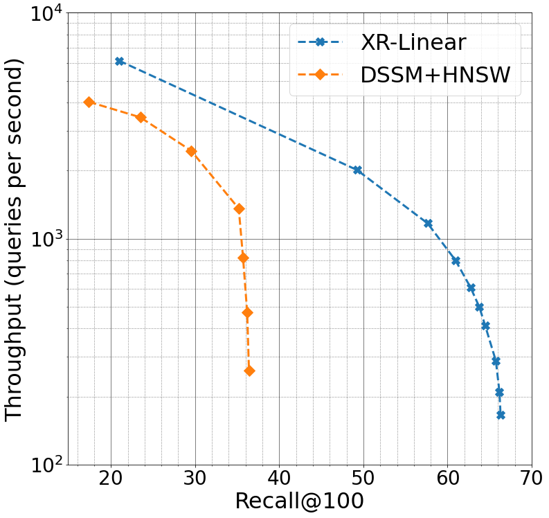
Figure 4. Throughput-Recall Trade-off comparison between XR-Linear (PECOS) and DSSM $+$HNSW. The curve of the latter method is obtained by sweeping the HNSW inference hyper-parameters $efS=\{10,50,100,250,500\}$.

Weight Pruning

As discussed in Section 3.3, we conduct element-wise weight pruning on the parameters of XR-Linear model trained on Unigram$+$Bigrams$+$Char Trigrams ($4.2M$) features. We experiment with the thresholds $\epsilon=\{0.1,0.2,0.3,0.35,0.4,0.45\}$, and the results are shown in Table 3.

From $\epsilon=0.1$ to $\epsilon=0.35$, the model size has a $3$x reduction (i.e., from $295$ GB to $90$ GB), having the same model size as the XR-Linear model trained on unigram ($3M$) features. Crucially, the pruned XR-Linear model still enjoys a sizable improvement over the XR-Linear model trained on unigram ($3M$) features, where the Recall$@100$ is $57.63\%$ versus $54.86\%$. While the real-time inference memory of XR-Linear closely follows its model disk space, the latter has smaller impact on the inference latency. In particular, from $\epsilon=0.1$ to $\epsilon=0.45$, the model size has a $5$x reduction (from $295$ GB to $62$ GB), while the inference latency reduced by only $32.5\%$ (from $1.20$ ms$/$q to $0.81$ ms$/$q). On the other hand, the inference beam search size has a larger impact on real-time inference latency, as we will discuss in the following paragraph.

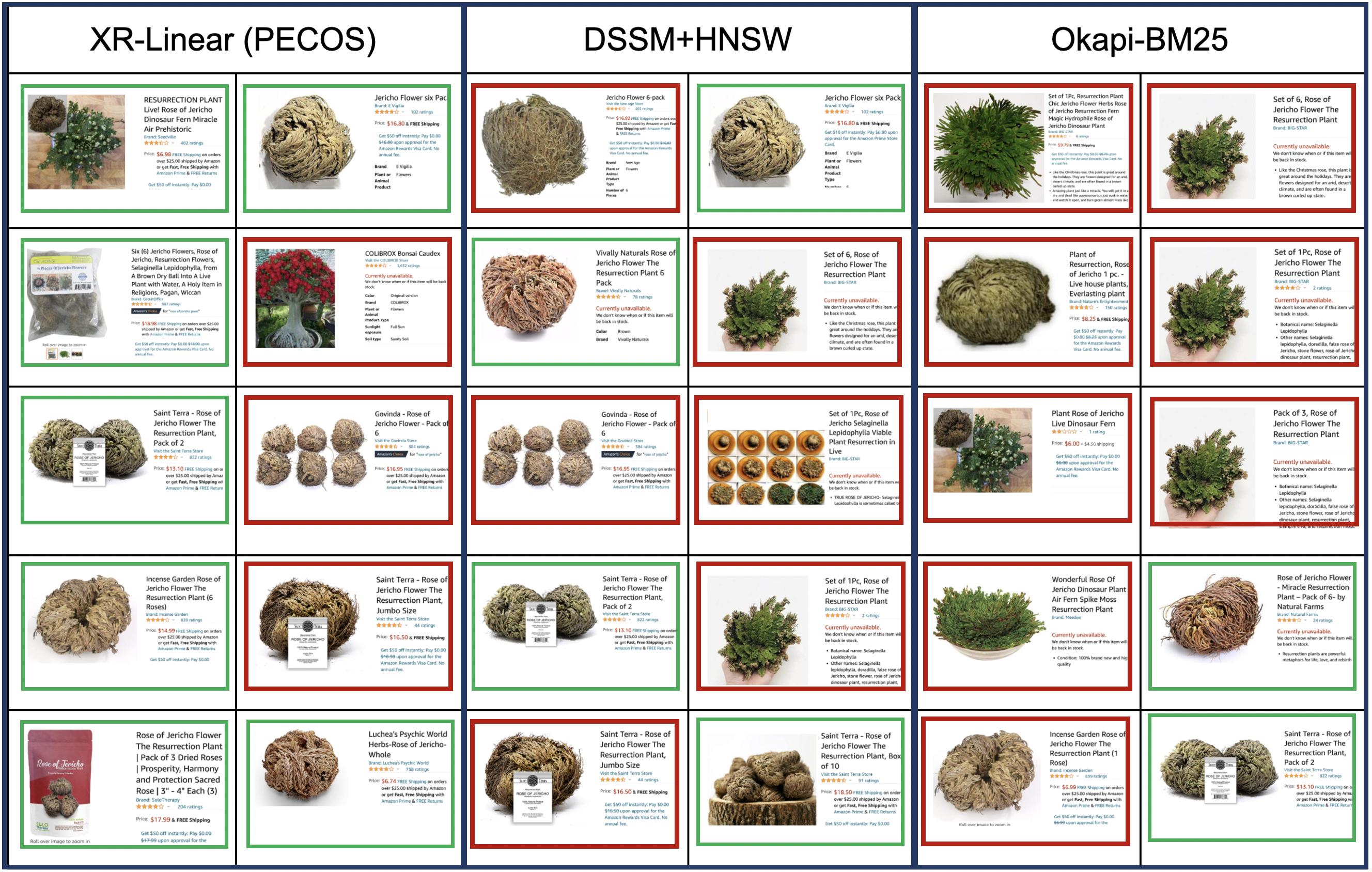
Figure 5. Side-by-side comparison of the retrieved products for XR-Linear (PECOS), DSSM $+$HNSW, and Okapi-BM25. The test query is ”rose of jericho plant”, and green box means there is at least one purchase while red box means no purchase.

Beam Size

We analyze how beam search size of XR-Linear prediction affects the Recall$@100$ and inference latency. The results are presented in Table 4. We also compare the throughput (i.e., inverse of latency, higher the better) versus Recall$@100$ for X-Linear and DSSM $+$ HNSW, as shown in Figure 4.

From beam size $b=1$ to $b=15$, we see a clear trade-off between Recall$@100$ and latency, where the former increases from $20.95\%$ to $60.94\%$, at the cost of $7x$ higher latency (from $0.16$ ms$/$q to $1.24$ ms$/$q). Real-world product search systems typically limit the real-time latency of matching algorithms to be smaller than $5$ ms$/$q. Therefore, even with $b=30$, the proposed XR-Linear approach is still highly applicable for the real-world online deployment setup.

In Figure 4, we also examine the throughput-recall trade-off for the embedding-based retrieval model DSSM (Nigam et al., 2019) that uses HNSW (Malkov and Yashunin, 2020) to do inference. XR-Linear outperforms DSSM $+$ HNSW significantly, with higher retrieval quality and larger throughput (smaller inference latency).

In Figure 5, we present the retrieved products for an example test query ”rose of jericho plant”, and compare the retrieval quality of XR-Linear (PECOS), DSSM $+$HNSW, and Okapi-BM25. From the top $10$ predictions (i.e., retrieved products), we see that XR-Linear covers more products that were purchased, and the retrieved set is more diverse, compared to the other two baselines.

4.5. Online Experiments

We conducted an online A/B test to experiment different semantic matching algorithms on a large-scale e-commerce retail product website. The control in this experiment is the traditional lexical-based matching augmented with candidates generated by DSSM. The treatment is the same traditional lexical-based matching, but augmented with candidates generated by XR-Linear instead. After a period of time, many key performance indicators of the treatment are statistically significantly higher than the control, which is consistent with our offline observations. We leave how to combine DSSM and XR-Linear to generate better match set for product search as future work.

5. Discussion and Future Work

In this work, we presented XR-Linear (PECOS), a tree-based XMC model to augment the match set for an online retail search system and improved product discovery with better recall rates. Specifically, to retrieve products from a $100$ million product catalog, the proposed solution achieves Recall@100 of $60.9\%$ with a low latency of $1.25$ millisecond per query (ms$/$q). Our tree-based linear models is robust to weight pruning which can flexibly meet different system memory or disk space requirements.

One challenge for our method is how to retrieve cold-start products with no training signal (e.g., no clicks nor purchases). One naive solution is to assign cold-start products into nearest relevant leaf node clusters based on distances between product embeddings and cluster centroids. We then use the average of existing product weight vectors which are the nearest neighbors of this novel product to induce the relevance score. This is an interesting setup and we leave it for future work.

References

- (1)
- Babbar and Schölkopf (2017) Rohit Babbar and Bernhard Schölkopf. 2017. DiSMEC: distributed sparse machines for extreme multi-label classification. In WSDM.
- Babbar and Schölkopf (2019) Rohit Babbar and Bernhard Schölkopf. 2019. Data scarcity, robustness and extreme multi-label classification. Machine Learning (2019), 1–23.
- Bhatia et al. (2016) K. Bhatia, K. Dahiya, H. Jain, A. Mittal, Y. Prabhu, and M. Varma. 2016. The extreme classification repository: Multi-label datasets and code. http://manikvarma.org/downloads/XC/XMLRepository.html
- Boytsov and Naidan (2013) Leonid Boytsov and Bilegsaikhan Naidan. 2013. Engineering efficient and effective non-metric space library. In International Conference on Similarity Search and Applications. Springer, 280–293.
- Boytsov and Nyberg (2020) Leonid Boytsov and Eric Nyberg. 2020. Flexible retrieval with NMSLIB and FlexNeuART. arXiv preprint arXiv:2010.14848 (2020).
- Chang et al. (2020a) Wei-Cheng Chang, Felix X. Yu, Yin-Wen Chang, Yiming Yang, and Sanjiv Kumar. 2020a. Pre-training Tasks for Embedding-based Large-scale Retrieval. In International Conference on Learning Representations.
- Chang et al. (2020b) Wei-Cheng Chang, Hsiang-Fu Yu, Kai Zhong, Yiming Yang, and Inderjit S Dhillon. 2020b. Taming Pretrained Transformers for Extreme Multi-label Text Classification. In Proceedings of the 26th ACM SIGKDD International Conference on Knowledge Discovery & Data Mining. 3163–3171.
- Chen et al. (2017) Danqi Chen, Adam Fisch, Jason Weston, and Antoine Bordes. 2017. Reading Wikipedia to Answer Open-Domain Questions. In Proceedings of the 55th Annual Meeting of the Association for Computational Linguistics (ACL) (Volume 1: Long Papers). 1870–1879.
- Covington et al. (2016) Paul Covington, Jay Adams, and Emre Sargin. 2016. Deep neural networks for Youtube recommendations. In Proceedings of the 10th ACM conference on recommender systems. 191–198.
- Craswell et al. (2020) Nick Craswell, Bhaskar Mitra, Emine Yilmaz, Daniel Campos, and Ellen M Voorhees. 2020. Overview of the TREC 2019 deep learning track. arXiv preprint arXiv:2003.07820 (2020).
- Devlin et al. (2019) Jacob Devlin, Ming-Wei Chang, Kenton Lee, and Kristina Toutanova. 2019. BERT: Pre-training of deep bidirectional transformers for language understanding. In Proceedings of the 2019 Conference of the North American Chapter of the Association for Computational Linguistics (NAACL).
- Dhillon and Modha (2001) Inderjit S Dhillon and Dharmendra S Modha. 2001. Concept decompositions for large sparse text data using clustering. Machine learning 42, 1-2 (2001), 143–175.
- Fan et al. (2008) Rong-En Fan, Kai-Wei Chang, Cho-Jui Hsieh, Xiang-Rui Wang, and Chih-Jen Lin. 2008. LIBLINEAR: A library for large linear classification. Journal of machine learning research 9, Aug (2008), 1871–1874.
- Gao et al. (2020) Luyu Gao, Zhuyun Dai, Zhen Fan, and Jamie Callan. 2020. Complementing lexical retrieval with semantic residual embedding. arXiv preprint arXiv:2004.13969 (2020).
- Guo et al. (2020) Ruiqi Guo, Philip Sun, Erik Lindgren, Quan Geng, David Simcha, Felix Chern, and Sanjiv Kumar. 2020. Accelerating large-scale inference with anisotropic vector quantization. In International Conference on Machine Learning. PMLR, 3887–3896.
- Guu et al. (2020) Kelvin Guu, Kenton Lee, Zora Tung, Panupong Pasupat, and Ming-Wei Chang. 2020. REALM: Retrieval-augmented language model pre-training. In Proceedings of the 37th International Conference on Machine Learning (Proceedings of Machine Learning Research, Vol. 119). 3929–3938.
- He et al. (2016) Kaiming He, Xiangyu Zhang, Shaoqing Ren, and Jian Sun. 2016. Deep residual learning for image recognition. In CVPR.
- Henderson et al. (2019) Matthew Henderson, Ivan Vulić, Daniela Gerz, Iñigo Casanueva, Paweł Budzianowski, Sam Coope, Georgios Spithourakis, Tsung-Hsien Wen, Nikola Mrkšić, and Pei-Hao Su. 2019. Training neural response selection for task-oriented dialogue systems. arXiv preprint arXiv:1906.01543 (2019).
- Huang et al. (2013) Po-Sen Huang, Xiaodong He, Jianfeng Gao, Li Deng, Alex Acero, and Larry Heck. 2013. Learning deep structured semantic models for web search using clickthrough data. In Proceedings of the 22nd ACM international conference on Information & Knowledge Management. 2333–2338.
- Jain et al. (2019) Himanshu Jain, Venkatesh Balasubramanian, Bhanu Chunduri, and Manik Varma. 2019. SLICE: Scalable Linear Extreme Classifiers Trained on 100 Million Labels for Related Searches. In Proceedings of the Twelfth ACM International Conference on Web Search and Data Mining. ACM, 528–536.
- Jasinska-Kobus et al. (2020) Kalina Jasinska-Kobus, Marek Wydmuch, Krzysztof Dembczynski, Mikhail Kuznetsov, and Robert Busa-Fekete. 2020. Probabilistic Label Trees for Extreme Multi-label Classification. arXiv preprint arXiv:2009.11218 (2020).
- Jiang et al. (2021) Ting Jiang, Deqing Wang, Leilei Sun, Huayi Yang, Zhengyang Zhao, and Fuzhen Zhuang. 2021. LightXML: Transformer with Dynamic Negative Sampling for High-Performance Extreme Multi-label Text Classification. In Proceedings of the AAAI Conference on Artificial Intelligence.
- Joulin et al. (2017) Armand Joulin, Edouard Grave, Piotr Bojanowski, and Tomas Mikolov. 2017. Bag of Tricks for Efficient Text Classification. In Proceedings of the 15th Conference of the European Chapter of the Association for Computational Linguistics (EACL): Volume 2, Short Papers. Association for Computational Linguistics, 427–431.
- Karpukhin et al. (2020) Vladimir Karpukhin, Barlas Oğuz, Sewon Min, Ledell Wu, Sergey Edunov, Danqi Chen, and Wen-Tau Yih. 2020. Dense passage retrieval for open-domain question answering. arXiv preprint arXiv:2004.04906 (2020).
- Khandagale et al. (2020) Sujay Khandagale, Han Xiao, and Rohit Babbar. 2020. BONSAI-Diverse and Shallow Trees for Extreme Multi-label Classification. Machine Learning (2020).
- Kuznetsova et al. (2020) Alina Kuznetsova, Hassan Rom, Neil Alldrin, Jasper Uijlings, Ivan Krasin, Jordi Pont-Tuset, Shahab Kamali, Stefan Popov, Matteo Malloci, Alexander Kolesnikov, et al. 2020. The open images dataset v4. International Journal of Computer Vision (2020), 1–26.
- Lee et al. (2019) Kenton Lee, Ming-Wei Chang, and Kristina Toutanova. 2019. Latent retrieval for weakly supervised open domain question answering. In Proceedings of the 57th Annual Meeting of the Association for Computational Linguistics (ACL).
- Malkov and Yashunin (2020) Y. A. Malkov and D. A. Yashunin. 2020. Efficient and Robust Approximate Nearest Neighbor Search Using Hierarchical Navigable Small World Graphs. IEEE Transactions on Pattern Analysis and Machine Intelligence 42, 4 (2020), 824–836.
- Manning et al. (2008) Christopher D. Manning, Prabhakar Raghavan, and Hinrich Schütze. 2008. Introduction to information retrieval. Cambridge University Press. https://doi.org/10.1017/CBO9780511809071
- Mazaré et al. (2018) Pierre-Emmanuel Mazaré, Samuel Humeau, Martin Raison, and Antoine Bordes. 2018. Training millions of personalized dialogue agents. In EMNLP.
- Nguyen et al. (2016) Tri Nguyen, Mir Rosenberg, Xia Song, Jianfeng Gao, Saurabh Tiwary, Rangan Majumder, and Li Deng. 2016. MS MARCO: A human generated machine reading comprehension dataset. In CoCo@ NIPS.
- Nigam et al. (2019) Priyanka Nigam, Yiwei Song, Vijai Mohan, Vihan Lakshman, Weitian Ding, Ankit Shingavi, Choon Hui Teo, Hao Gu, and Bing Yin. 2019. Semantic product search. In Proceedings of the 25th ACM SIGKDD International Conference on Knowledge Discovery & Data Mining. 2876–2885.
- Prabhu et al. (2018) Yashoteja Prabhu, Anil Kag, Shrutendra Harsola, Rahul Agrawal, and Manik Varma. 2018. Parabel: Partitioned label trees for extreme classification with application to dynamic search advertising. In WWW.
- Prabhu et al. (2020) Yashoteja Prabhu, Aditya Kusupati, Nilesh Gupta, and Manik Varma. 2020. Extreme regression for dynamic search advertising. In Proceedings of the 13th International Conference on Web Search and Data Mining. 456–464.
- Reddi et al. (2019) Sashank J Reddi, Satyen Kale, Felix Yu, Dan Holtmann-Rice, Jiecao Chen, and Sanjiv Kumar. 2019. Stochastic Negative Mining for Learning with Large Output Spaces. In AISTATS.
- Robertson et al. (2009) Stephen Robertson, Hugo Zaragoza, et al. 2009. The probabilistic relevance framework: BM25 and beyond. Foundations and Trends® in Information Retrieval 3, 4 (2009), 333–389.
- Robertson and Walker (1994) Stephen E Robertson and Steve Walker. 1994. Some simple effective approximations to the 2-Poisson model for probabilistic weighted retrieval. In SIGIR’94. Springer, 232–241.
- Song et al. (2020) Liuyihan Song, Pan Pan, Kang Zhao, Hao Yang, Yiming Chen, Yingya Zhang, Yinghui Xu, and Rong Jin. 2020. Large-Scale Training System for 100-Million Classification at Alibaba. In Proceedings of the 26th ACM SIGKDD International Conference on Knowledge Discovery & Data Mining. 2909–2930.
- Tagami (2017) Yukihiro Tagami. 2017. AnnexML: Approximate nearest neighbor search for extreme multi-label classification. In Proceedings of the 23rd ACM SIGKDD international conference on knowledge discovery and data mining. 455–464.
- Trotman et al. (2014) Andrew Trotman, Antti Puurula, and Blake Burgess. 2014. Improvements to BM25 and language models examined. In Proceedings of the 2014 Australasian Document Computing Symposium. 58–65.
- Vaswani et al. (2017) Ashish Vaswani, Noam Shazeer, Niki Parmar, Jakob Uszkoreit, Llion Jones, Aidan N Gomez, Łukasz Kaiser, and Illia Polosukhin. 2017. Attention is all you need. In NIPS.
- Weinberger et al. (2009) Kilian Weinberger, Anirban Dasgupta, John Langford, Alex Smola, and Josh Attenberg. 2009. Feature hashing for large scale multitask learning. In Proceedings of the 26th annual international conference on machine learning. 1113–1120.
- Wolf et al. ([n.d.]) Thomas Wolf, Julien Chaumond, Lysandre Debut, Victor Sanh, Clement Delangue, Anthony Moi, Pierric Cistac, Morgan Funtowicz, Joe Davison, Sam Shleifer, et al. [n.d.]. HuggingFace Transformer Benchmarking. https://huggingface.co/transformers/benchmarks.html. Accessed: 2021-02-08.
- Wolf et al. (2020) Thomas Wolf, Julien Chaumond, Lysandre Debut, Victor Sanh, Clement Delangue, Anthony Moi, Pierric Cistac, Morgan Funtowicz, Joe Davison, Sam Shleifer, et al. 2020. Transformers: State-of-the-art natural language processing. In Proceedings of the 2020 Conference on Empirical Methods in Natural Language Processing: System Demonstrations. 38–45.
- Wydmuch et al. (2018) Marek Wydmuch, Kalina Jasinska, Mikhail Kuznetsov, Róbert Busa-Fekete, and Krzysztof Dembczynski. 2018. A no-regret generalization of hierarchical softmax to extreme multi-label classification. In NIPS.
- Xiong et al. (2021) Lee Xiong, Chenyan Xiong, Ye Li, Kwok-Fung Tang, Jialin Liu, Paul Bennett, Junaid Ahmed, and Arnold Overwijk. 2021. Approximate nearest neighbor negative contrastive learning for dense text retrieval. In ICLR.
- Yang et al. (2020) Ji Yang, Xinyang Yi, Derek Zhiyuan Cheng, Lichan Hong, Yang Li, Simon Xiaoming Wang, Taibai Xu, and Ed H Chi. 2020. Mixed Negative Sampling for Learning Two-tower Neural Networks in Recommendations. In Companion Proceedings of the Web Conference 2020. 441–447.
- Yen et al. (2017) Ian EH Yen, Xiangru Huang, Wei Dai, Pradeep Ravikumar, Inderjit S. Dhillon, and Eric Xing. 2017. PPDsparse: A parallel primal-dual sparse method for extreme classification. In KDD. ACM.
- Yen et al. (2016) Ian EH Yen, Xiangru Huang, Kai Zhong, Pradeep Ravikumar, and Inderjit S Dhillon. 2016. PD-Sparse: A Primal and Dual Sparse Approach to Extreme Multiclass and Multilabel Classification. In International Conference on Machine Learning (ICML).
- Yi et al. (2019) Xinyang Yi, Ji Yang, Lichan Hong, Derek Zhiyuan Cheng, Lukasz Heldt, Aditee Kumthekar, Zhe Zhao, Li Wei, and Ed Chi. 2019. Sampling-bias-corrected neural modeling for large corpus item recommendations. In Proceedings of the 13th ACM Conference on Recommender Systems. 269–277.
- You et al. (2019) Ronghui You, Zihan Zhang, Ziye Wang, Suyang Dai, Hiroshi Mamitsuka, and Shanfeng Zhu. 2019. AttentionXML: Label Tree-based Attention-Aware Deep Model for High-Performance Extreme Multi-Label Text Classification. In Advances in Neural Information Processing Systems. 5812–5822.
- Yu et al. (2020) Hsiang-Fu Yu, Kai Zhong, and Inderjit S Dhillon. 2020. PECOS: Prediction for Enormous and Correlated Output Spaces. arXiv preprint arXiv:2010.05878 (2020).
- Zobel and Moffat (2006) Justin Zobel and Alistair Moffat. 2006. Inverted files for text search engines. ACM computing surveys (CSUR) 38, 2 (2006), 6–es.