Black Box Variational Bayesian Model Averaging

Abstract

For many decades now, Bayesian Model Averaging (BMA) has been a popular framework to systematically account for model uncertainty that arises in situations when multiple competing models are available to describe the same or similar physical process. The implementation of this framework, however, comes with a multitude of practical challenges including posterior approximation via Markov Chain Monte Carlo and numerical integration. We present a Variational Bayesian Inference approach to BMA as a viable alternative to the standard solutions which avoids many of the aforementioned pitfalls. The proposed method is “black box” in the sense that it can be readily applied to many models with little to no model-specific derivation. We illustrate the utility of our variational approach on a suite of examples and discuss all the necessary implementation details. Fully documented Python code with all the examples is provided as well.

Keywords: Bayesian inference; Model uncertainty; Model selection; Markov Chain Monte Carlo; Model evidence; Variational Bayes

1 Introduction

The existence of several competing models to solve the same or similar problem is a common scenario across scientific applications. One typically encounters a slew of candidate models during standard regression analysis with multiple predictors. Another widely familiar example is a numerical weather prediction with multitudes of forecasting models available. The routine practice in this situation is to select a single model and then make inference based on this model which ignores a major component of uncertainty - model uncertainty (Leamer, 1978). Bayesian model averaging (BMA) is the natural Bayesian framework to systematically account for uncertainty due to several competing models.

For any quantity of interest $\bm{\Delta}$, such as a future observation or an effect size, the BMA posterior density $p(\bm{\Delta}|\bm{d})$ corresponds to the mixture of posterior densities of the individual models $p(\bm{\Delta}|\bm{d},M)$ weighted by their posterior model probabilities $p(M|\bm{d})$:

$$p(\bm{\Delta}|\bm{d})=\sum_{M\in\mathcal{M}}p(\bm{\Delta}|\bm{d},M)p(M|\bm{d}),$$ (1)

where $\mathcal{M}$ denotes the space of all models, $\bm{d}=(d_{1},\cdots,d_{n})$ are given datapoints, and $d_{i}=(x_{i},y_{i})$ for $i=1,\dots,n$ are input-observation pairs. Note, if the space of models is $\mathcal{M}=\{M_{1},\cdots,M_{K}\}$, then the formula in (1) can be equivalenty written as $p(\bm{\Delta}|\bm{d})=\sum_{k=1}^{K}p(\bm{\Delta}|\bm{d},M_{k})p(M_{k}|\bm{d})$ which is a more commonly used notation for BMA. We stick to the notation in (1) to facilitate the developments in section 2.2

The posterior probability of a model $M$ is given by a simple application of the Bayes’ theorem:

$$p(M|\bm{d})=\frac{p(\bm{d}|M)p(M)}{\sum_{M^{\prime}\in\mathcal{M}}p(\bm{d}|M^{\prime})p(M^{\prime})}.$$ (2)

Due to the mixture form of the density (1), determining these probabilities is the key to successful implementation of the BMA framework. To do so, one first needs to assign a suitable prior probability $p(M)$ that $M$ is the true model (assuming there is one such, among the models considered). Hoeting et al. (1999) notes that,

When there is little prior information about the relative plausibility of the models considered, the assumption that all models are equally likely a priory is a reasonable “neutral” choice.

One can, nevertheless, choose informative prior distributions when prior information about the likelihood of each model is available. Eliciting an informative prior is a non-trivial task, but Madigan et al. (1995) provide some guidance in the context of graphical models that can be applied in other settings as well.

The second component of model’s posterior probability is the model’s marginal likelihood, also known as model evidence,

$$p(\bm{d}|M)=\int p(\bm{d}|\bm{\theta}_{M},M)p(\bm{\theta}_{M}|M)\mathop{}\!\textrm{d}\bm{\theta}_{M},$$ (3)

where $\bm{\theta}_{M}$ is the set of model-specific parameters ($\bm{\theta}_{M}=(\bm{\beta},\sigma)$ in regression problems), $p(\bm{\theta}_{M}|M)$ is their prior distribution, and $p(\bm{d}|\bm{\theta}_{M},M)$ is the model’s data likelihood. The evaluation of model evidence is one of the main reasons why BMA becomes computationally challenging in practice, because a closed form solution is available only in special scenarios for the exponential family of distributions with conjugate priors, and thus the integral (3) requires approximation. Some problem-specific algorithms have been developed for direct sampling from BMA posterior density (1) such as the Markov chain Monte Carlo (MCMC) model composition for linear regression models (MC³) (Raftery et al., 1997).

A vast body of literature was produced over the past 30 years on the topic of model evidence approximation, with the simplest approach being the Monte Carlo (MC) integration. The advantage of MC integration is in the method’s ease of implementation, however, one typically needs to generate a large number of samples from prior distribution to achieve reasonable convergence. A popular improvement to the simple MC integration is the harmonic mean estimator which makes the use of samples from posterior distribution of model parameters and therefore converges more quickly. On the other hand, it can be unstable, and it tends to overestimate the evidence (see Raftery et al. (2007); Lenk (2009)). A large class of statistically efficient estimators is based on importance sampling that relies on draws from an importance density which approximates the joint posterior density of model parameters. However, a poor choice of importance density may lead to a huge loss of efficiency. See Neal (2001), Friel and Pettitt (2008), and Pajor (2017) for some examples of estimators with importance sampling. Another classical method is the Laplace approximation. This corresponds to a second order Taylor expansion of the log-likelihood around its maximum, which makes the likelihood normal. Laplace method is efficient for well behaved likelihoods. We refer the reader to Kass and Raftery (1995); Ardia et al. (2012) and Friel and Wyse (2012) for a complete survey of popular approximation methods for the model evidence. Additionally, the more recently proposed Nested Sampling algorithm by Skilling (2006) and expanded by Feroz et al. (2009) provides another alternative to the aforementioned approaches.

Here we want to point out that the definition of BMA relies on the assumption that the true model which represents the physical reality is within the models being considered (i.e. $\mathcal{M}$-closed setting). BMA can lead to misleading results when the true model is not included (i.e. $\mathcal{M}$-open setting). For instance, a scenario with two models – one mediocre and one ”perfect” almost everywhere with a large deviation from the truth at a single point of the input space – will typically result in the selection of the mediocre model. Similarly, BMA can also lead to a suboptimal performance under model misspecification (Clarke, 2003; Masegosa, 2020). Using BMA in the $\mathcal{M}$-open setting additionally creates a logical tension between interpreting $p(M|\bm{d})$ and $p(M)$ as probabilities of $M$ being the true model and knowing that the true model is not in $\mathcal{M}$. One can perhaps reconcile this tension by considering $p(M|\bm{d})$ and $p(M)$ as the probabilities of $M$ being a useful description of physical reality. In what follows, we will assume that the reader is comfortable with assigning a prior over $\mathcal{M}$, even in the $\mathcal{M}$-open setting. We refer to Bernardo and Smith (1994) for a detailed discussion about the conceptual differences between the $\mathcal{M}$-closed and $\mathcal{M}$-open settings and to Fragoso et al. (2018) for a recent survey of BMA methodology. A decision-theoretic approach to account for model uncertainty in $\mathcal{M}$-open setting is presented in Clyde and Iversen (2013). Recently, Phillips et al. (2021) proposed a model-mixing approach for the case when the list of models considered does not contain the true model. Both of these methods address the inadequacy of BMA in $\mathcal{M}$-open setting by not considering models as an extension of the parameter space.

Despite its conceptual and computational challenges, BMA has a long history of use in both natural sciences and humanities because of a superior predictive performance that is theoretically guaranteed (Bernardo and Smith, 1994). Geweke (1999) introduced BMA in economics and later in other fields such as political and social sciences. See the recent review on the use of BMA in Economics by Steel (2020). BMA has also been applied to the medical sciences (Balasubramanian et al., 2014; Schorning et al., 2016), ecology and evolution (Silvestro et al., 2014; Hooten and Hobbs, 2015), genetics (Wei et al., 2011; Wen, 2015), machine learning (Clyde et al., 2011; Hernández et al., 2018; Mukhopadhyay and Dunson, 2020), and lately in nuclear physics (Neufcourt et al., 2019, 2020a, 2020b; Kejzlar et al., 2020).

In this paper, we present a Variational Bayesian Inference (VBI) approach to BMA. VBI is a useful alternative to the sampling-based approximation via MCMC that approximates a target density through optimization. Statisticians and computer scientists (starting with Peterson and Anderson (1987); Jordan et al. (1999)) have been widely using variational techniques because they tend to be faster and easier to scale to massive datasets. Our method is based on the variational inference algorithm with reparametrization gradients developed by Titsias and Lázaro-Gredilla (2014) and Kucukelbir et al. (2017) which can be applied to many models with minimum additional derivations. The proposed approach, which we shall call the black box variational BMA (VBMA), is a one step procedure that simultaneously approximates model evidences and posterior distributions of individual models while enjoying all the advantages (and disadvantages) of VBI. Here we note that this is not the first time a VBI is used in the context of BMA. For instance, Latouche and Robin (2016) developed a variational Bayesian approach specifically for averaging of graphon functions, and Jaureguiberry et al. (2014) use VBI and BMA for audio source separation. However, the VBMA is a general algorithm that can be applied directly to a wide class of models including Bayesian neural networks, generalized linear models, and Gaussian process models.

1.1 Outline of this paper

In section 2, we provide a brief overview of VBI and derive our proposed VBMA algorithm. Then, in section 3, we present a collection of examples that include standard linear regression, logistic regression, and Bayesian model selection. To fully showcase the computational benefits of VBMA, we consider Gaussian process models for residuals of separation energies of atomic nuclei. We compare VBMA with direct sampling BMA via MC³ and with MCMC posterior approximation and evidence computed using MC integration. A fully documented Python code with our algorithm and examples is available at https://github.com/kejzlarv/BBVBMA. Lastly, in section 4, we discuss the pros and cons of VBMA and provide a list of sensible machine learning applications for the proposed methodology.

2 BMA via Variational Bayesian Inference

2.1 Variational Bayesian Inference

VBI strives to approximate a target posterior distribution through optimization. One first considers a family of distributions $q(\bm{\theta}|\bm{\lambda})$, indexed by a variational parameter $\bm{\lambda}$, over the space of model parameters and subsequently finds a member of this family $q^{*}$ closest to the posterior distribution $p(\bm{\theta}|\bm{d})$. The simplest variational family is the mean-field family which assumes independence of all the components in $\bm{\theta}$ but many other families of variational distributions exist; see Wainwright and Jordan (2008); Hoffman and Blei (2015); Ranganath et al. (2016); Tran et al. (2015, 2017); Rezende and Mohamed (2015); Kingma et al. (2016); Kucukelbir et al. (2017); Fortunato et al. (2017); Papamakarios et al. (2017, 2021); Kobyzev et al. (2021); Weilbach et al. (2020). The recent work of Ambrogioni et al. (2021) and the references therein provide a detailed discussion of these class of variational families and their associated implementation challenges. The approximate distribution $q^{*}$ is chosen to minimize the Kullback-Leibler (KL) divergence of $q(\bm{\theta}|\bm{\lambda})$ from $p(\bm{\theta}|\bm{d})$:

$$q^{*}=\operatorname*{argmin}_{q(\bm{\theta}|\bm{\lambda})}KL(q(\bm{\theta}|\bm{\lambda})||p(\bm{\theta}|\bm{d})).$$ (4)

Finding $q^{*}$ is done in practice by maximizing an equivalent objective function (Jordan et al., 1999), the evidence lower bound (ELBO):

$$\mathcal{L}(q)=\mathbb{E}_{q(\bm{\theta}|\bm{\lambda})}\bigg{[}\log p(\bm{d},\bm{\theta})-\log q(\bm{\theta}|\bm{\lambda})\bigg{]}.$$ (5)

The ELBO is the sum between the negative KL divergence of the variational distribution from the true posterior distribution and the log of the marginal data distribution $p(\bm{d})$. The term $\log p(\bm{d})$ is constant with respect to $q(\bm{\theta}|\bm{\lambda})$. It is also a lower bound on $\log p(\bm{d})$ for any choice of $q(\bm{\theta}|\bm{\lambda})$. ELBO can be optimized via standard coordinate- or gradient-ascent methods. However, these techniques are inefficient for large datasets, and so it has become common practice to use the stochastic gradient ascent (SGA) algorithm. SGA updates $\bm{\lambda}$ at the $t^{th}$ iteration according to

$$\bm{\lambda}_{t+1}\leftarrow\bm{\lambda}_{t}+\rho_{t}\tilde{l}(\bm{\lambda}_{t}),$$ (6)

where $\tilde{l}(\bm{\lambda})$ is a realization of the random variable $\tilde{\mathcal{L}}(\bm{\lambda})$ which is an unbiased estimate of the gradient $\nabla_{\bm{\lambda}}\mathcal{L}(\bm{\lambda})$.

Let us now assume that $\log p(\bm{d},\bm{\theta})$ and $\log q(\bm{\theta}|\bm{\lambda})$ are differentiable functions with respect to $\bm{\theta}$, and that the random variable $\bm{\theta}$ can be reparametrized using a differentiable transformation $t(\bm{z},\bm{\lambda})$ of an auxiliary variable $\bm{z}$ so that $\bm{z}\sim\psi(\bm{z})$ and $\bm{\theta}=t(\bm{z},\bm{\lambda})$ imply $\bm{\theta}\sim q(\bm{\theta}|\bm{\lambda})$. It is assumed that $\psi(\bm{z})$ exists in a standard form so that any parameter mean vector is set to zero and scale parameters are set to one. For example, if we consider a real valued $\theta$ with normal variation family $q(\theta|\mu,\sigma^{2})$, then $t(z,(\mu,\sigma))=z\sigma+\mu$ and $z\sim\text{Normal}(0,1)$. Note that the variational parameters are part of the transformation and not the auxiliary distribution. The gradient of the ELBO can be then expressed as the following expectation with respect to the auxiliary distribution $\psi(\bm{z})$ (Titsias and Lázaro-Gredilla, 2014; Kucukelbir et al., 2017):

$$\nabla_{\bm{\lambda}}\mathcal{L}(q)=\mathbb{E}_{\psi(\bm{z})}\bigg{[}\nabla_{\bm{\theta}}(\log p(\bm{d},\bm{\theta})-\log q(\bm{\theta}|\bm{\lambda}))\times\nabla_{\bm{\lambda}}t(\bm{z},\bm{\lambda})\bigg{]}.$$ (7)

The expectation (7) does not have a closed form in general, nevertheless, one can use $S$ samples from $\psi(\bm{z})$ to construct its unbiased MC estimate for the SGA (6)

$$\tilde{l}(\bm{\lambda})=\frac{1}{S}\sum^{S}_{s=1}\bigg{[}\nabla_{\bm{\theta}}(\log p(\bm{d},t(\bm{z}[s],\bm{\lambda}))-\log q(t(\bm{z}[s],\bm{\lambda})|\bm{\lambda}))\times\nabla_{\bm{\lambda}}t(\bm{z}[s],\bm{\lambda})\bigg{]},$$ (8)

where $\bm{z}[s]\sim\psi(\bm{z})$. Since that the differentiability assumptions and the reparametrization trick allows the use of autodifferentiation to take gradients, the method is black box in nature (Kucukelbir et al., 2017). The disadvantage of reparametrization gradient is that it requires differentiable models, i.e, models with no discrete variables. One can use the so called score gradient (Ranganath et al., 2014) for models with discrete variables which is also black box in nature, however, the variance of the gradient estimates can be large and lead to unreliable results (Ruiz et al., 2016). The estimate (8) can be conveniently used in the SGA algorithm which converges to a local maximum of $\mathcal{L}(\bm{\lambda})$ (global for $\mathcal{L}(\bm{\lambda})$ concave (Bottou et al., 1997)) when the learning rate $\rho_{t}$ follows the Robbins-Monro conditions (Robbins and Monro, 1951)

$$\sum_{t=1}^{\infty}\rho_{t}=\infty,\hskip 28.45274pt\sum_{t=1}^{\infty}\rho^{2}_{t}<\infty.$$ (9)

Choosing an optimal learning rate $\rho_{t}$ can be challenging in practice. Ideally, one would want the rate to be small in situations where MC estimates of the ELBO gradient are erratic (large variance) and large when the MC estimates are relatively stable (small variance). The elements of variational parameter $\lambda$ can also differ in scale, and the selected learning rate should accommodate these varying, potentially small, scales. The ever increasing abundance of stochastic optimization in machine learning applications spawned development of numerous algorithms for element-wise adaptive scale learning rates. We use the Adam algorithm (Kingma and Ba, 2014) which is a popular and easy-to-implement adaptive rate algorithm. However, there are many other frequently used algorithms such as the AdaGrad (Duchi et al., 2011), the ADADELTA (Zeiler, 2012), or the RMSprop (Tieleman and Hinton, 2012). The step size associated with Adam is kept constant throughout the paper. However, as pointed out in Shazeer and Stern (2018), one may achieve a better performance by making use of linear ramp-up followed by some form of decay (Vaswani et al., 2017). In the Supplement, we provide the results based on RMSprop for comparison. We did not observe significant differences between RMSprop and Adam for the examples in section 3.

Below, we extend the standard VBI that approximates a distribution of model parameters to a scenario where a distribution over the model space needs to be also approximated.

2.2 Black Box Variational BMA

For any quantity of interest $\bm{\Delta}$, such as a future observation or an effect size, the BMA posterior density $p(\bm{\Delta}|\bm{d})$ corresponds to the mixture of posterior densities of the individual models $p(\bm{\Delta}|\bm{d},M)$ weighted by their posterior model probabilities $p(M|\bm{d})$ as in equations (1), (2), and (3).

In order to facilitate variational inference, we reformulate the problem of BMA as follows

$$p(\bm{\Delta}|\bm{d})=\int p(\bm{\Delta}|\bm{d},M,\bm{\theta}_{M})p(M,\bm{\theta}_{M}|\bm{d})\mathop{}\!\textrm{d}\mu(M,\bm{\theta}_{M})$$ (10)

where $\mu$ is the product measure of counting and Lebesgue. Note, the expression (10) indeed summarizes the equations (1), (2) and (3) in one step. In practice, the most difficult quantity to compute is $p(M,\bm{\theta}_{M}|\bm{d})$. We shall now consider the joint posterior distribution of the model $M$ and its corresponding parameter $\bm{\theta}_{M}$ as our parameter of interest. Note, the above notation allows for the dependence of $\bm{\theta}$ on the model $M$. This is needed as the indexing parameter of each model could differ in dimension, distribution, etc. As explained in Section 2, there has been a plethora of literature in using variational inference to obtain the posterior distribution $\bm{\theta}$ for a given model. In this section, we adapt the variational inference to obtain the joint distribution of the model and the parameter together in one stroke.

We next assume a variational approximation to the posterior distribution $p(M,\bm{\theta}_{M}|\bm{d})$ of the form $q(M,\bm{\theta}_{M}|\bm{\lambda}_{M})=q(M)q(\bm{\theta}_{M}|M,\bm{\lambda}_{M})$, where $q(M)$ is the variational model weight of model $M$ and $q(\bm{\theta}_{M}|\bm{\lambda}_{M})$ is the variational distribution of $\bm{\theta}_{M}$ under model $M$ and is indexed by its corresponding variational parameter $\bm{\lambda}_{M}$. Note that we treat $(M,\bm{\theta}_{M})$ as a random variable which takes on the values $(m,\bm{\theta}_{m})$ for varying values of $m\in\mathcal{M}=\{M_{1},\cdots,M_{K}\}$. The density of this random variable is given by $p(m,\bm{\theta}_{m}|\bm{d})$ under the true posterior, and by $q(m)q(\bm{\theta}_{m}|\bm{\lambda}_{m})$ under the variational posterior. Here $q(m)$ for $m\in\mathcal{M}$ can be any categorical distribution satisfying $\sum_{m\in\mathcal{M}}q(m)=1$. For each $m\in\mathcal{M}$, $q(\bm{\theta}_{m}|\bm{\lambda}_{m})$ can be any parametric distribution indexed by the parameters $\bm{\lambda}_{m}$. Possible choices of $q(\bm{\theta}_{m}|\bm{\lambda}_{m})$ include but are not restricted to mean field variational family of the form $q(\bm{\theta}_{m}|\bm{\lambda}_{m})=\prod_{i}q(\theta_{m}^{i}|\lambda_{m}^{i})$. We additionally assume that $\bm{\theta}_{M}$ can be reparametrized using a differentiable transformation $t(\bm{z}_{M},\bm{\lambda}_{M})$ of an auxiliary variable $\bm{z}_{M}$ so that $\bm{z}_{M}\sim\psi(\bm{z}_{M})$ and $\bm{\theta}_{M}=t(\bm{z}_{M},\bm{\lambda}_{M})$. We avoid the inherent dependence of $t(\cdot)$ on $M$ to simplify the notation.

Thus, the optimal variational distribution $q^{*}$ is given by

$$q^{*}=\operatorname*{argmin}_{q}KL(q(M,\bm{\theta}_{M}|\bm{\lambda}_{M})||p(M,\bm{\theta}_{M}|\bm{d})).$$ (11)

Again, in the KL expression above, we assume that $M$ is a random variable whose values are the individual models in the model space $\mathcal{M}$. As explained in section 2, finding $q^{*}$ is obtained in practice by maximizing an equivalent objective function (Jordan et al., 1999), the ELBO

$$\mathcal{L}(q)=\mathbb{E}_{q(M,\bm{\theta}_{M}|\bm{\lambda}_{M})}\bigg{[}\log p(\bm{d},M,\bm{\theta}_{M})-\log q(M,\bm{\theta}_{M}|\bm{\lambda}_{M})\bigg{]},$$ (12)

this time, subject to constraint $\sum_{M\in\mathcal{M}}q(M)=1$. Since $q(\bm{\theta}_{M}|\bm{\lambda}_{M})$ is a parametric family indexed by the parameters $\bm{\lambda}_{M}$, it is indeed a valid density function. However, since the categorical distribution $q(M)$ has freely varying parameters, the constraint $\sum_{M\in\mathcal{M}}q(M)=1$ is imposed. To accommodate the constraint, using Lagrange multipliers, we optimize

$$\mathcal{L}(q)=\mathbb{E}_{q(M,\bm{\theta}_{M}|\bm{\lambda}_{M})}[\log p(\bm{d},M,\bm{\theta}_{M})-\log q(M,\bm{\theta}_{M}|\bm{\lambda}_{M})]-\varrho(\sum_{M\in\mathcal{M}}q(M)-1).$$

The ELBO can be simplified further

$$\mathbb{E}_{q(M,\bm{\theta}_{M}|\lambda_{M})}[\log p(\bm{d},M,\bm{\theta}_{M})-\log q(M,\bm{\theta}_{M}|\bm{\lambda}_{M})]-\varrho(\sum_{M\in\mathcal{M}}q(M)-1)$$

$$=\mathbb{E}_{q(M,\bm{\theta}_{M}|\lambda_{M})}[\log p(\bm{d}|M,\bm{\theta}_{M})+\log p(\bm{\theta}_{M}|M)+\log p(M)$$

$$\enskip\qquad\qquad\qquad-\log q(\bm{\theta}_{M}|M,\bm{\lambda}_{M})-\log q(M)]-\varrho(\sum_{M\in\mathcal{M}}q(M)-1)$$

$$=\sum_{M\in\mathcal{M}}q(M)\mathbb{E}_{q(\bm{\theta}_{M}|M,\bm{\lambda}_{M})}[\log p(\bm{d}|M,\bm{\theta}_{M})+\log p(\bm{\theta}_{M}|M)+\log p(M)$$

$$\enskip\enskip\qquad\qquad\qquad\qquad\qquad-\log q(\bm{\theta}_{M}|M,\bm{\lambda}_{M})-\log q(M)]-\varrho(\sum_{M\in\mathcal{M}}q(M)-1).$$

Since the parameters $q(M)$ for $M\in\mathcal{M}$ do not depend on the variational parameters $\bm{\lambda}_{M}$, therefore $\nabla_{\lambda_{M}}\varrho(\sum_{M\in\mathcal{M}}q(M)-1)=0$. Thus, one obtains $\nabla_{\lambda_{M}}\mathcal{L}(q)=q(M)\mathcal{G}_{M}$ where

$${\mathcal{G}_{M}} =\mathbb{E}_{\psi(\bm{z}_{M})}[\nabla_{\bm{\theta}_{M}}(\log p(\bm{d}|M,\bm{\theta}_{M})+\log p(\bm{\theta}_{M}|M)-\log q(\bm{\theta}_{M}|M,\bm{\lambda}_{M}))\times\nabla_{\bm{\lambda}_{M}}t(\bm{z}_{M},\bm{\lambda}_{M})].$$

To estimate the quantity $\mathcal{G}_{M}$, we can generate multiple samples from the distribution $\psi(\bm{z}_{M})$ and then use the MC estimate

$$\widehat{\mathcal{G}}_{M}=\frac{1}{S}\sum_{s=1}^{S}[\nabla_{\bm{\theta}_{M}} (\log p(\bm{d}|M,t(\bm{z}_{M}[s],\bm{\lambda}_{M}))+\log p(t(\bm{z}_{M}[s],\bm{\lambda}_{M})|M)$$

$$-\log q(t(\bm{z}_{M}[s],\bm{\lambda}_{M})|M,\bm{\lambda}_{M}))\times\nabla_{\bm{\lambda}_{M}}t(\bm{z}_{M}[s],\bm{\lambda}_{M})].$$

To derive the update of $q(M)$, note that

$$\nabla_{q(M)}\mathcal{L}(q) =\underbrace{\mathbb{E}_{q(\bm{\theta}_{M}|M,\bm{\lambda}_{M})}[(\log p(\bm{d}|M,\bm{\theta}_{M})+\log p(\bm{\theta}_{M}|M)-\log q(\bm{\theta}_{M}|M,\bm{\lambda}_{M}))]}_{\mathcal{L}_{M}}$$

$$+\log p(M)-\log q(M)-1-\varrho,$$

where $\mathcal{L}_{M}$ is nothing but the ELBO under a fixed model $M$. Equating the above derivative to 0, we get a closed form expression for $q(M)$ as

$$q(M)=\exp(\mathcal{L}_{M}+\log p(M)-1-\varrho)\propto\exp(\mathcal{L}_{M}+\log p(M)).$$

It only remains to generate the quantity $\mathcal{L}_{M}$, which we get again by multiple samples from the distribution $\psi(\bm{z}_{M})$ and then use the MC estimate

$$\widehat{\mathcal{L}}_{M}=\frac{1}{S}\sum_{s=1}^{S}[\log p(\bm{d}|M,t(\bm{z}_{M}[s],\bm{\lambda}_{M}))+\log p(t(\bm{z}_{M}[s],\bm{\lambda}_{M})|M)-\log q(t(\bm{z}_{M}[s],\bm{\lambda}_{M})|M,\bm{\lambda}_{M})].$$

This allows us to get Algorithm 1 for VBMA.

Algorithm 1 Black Box Variational BMA

  Start with an initial choice of $(\bm{\lambda}_{M},q(M))_{M\in\mathcal{M}}$ and a learning rate $\rho$.

  repeat

     By generating $\bm{z}_{M}[1],\cdots,\bm{z}_{M}[S]$ from $\psi(\bm{z}_{M})$, calculate

$$\widehat{\mathcal{G}}_{M}=\frac{1}{S}\sum_{s=1}^{S}[\nabla_{\bm{\theta}_{M}} (\log p(\bm{d}|M,t(\bm{z}_{M}[s],\bm{\lambda}_{M}))+\log p(t(\bm{z}_{M}[s],\bm{\lambda}_{M})|M)$$

$$-\log q(t(\bm{z}_{M}[s],\bm{\lambda}_{M})|M,\bm{\lambda}_{M}))\times\nabla_{\bm{\lambda}_{M}}t(\bm{z}_{M}[s],\bm{\lambda}_{M})]$$

     Update $\bm{\lambda}_{M}$ as

$$\bm{\lambda}_{M}=\bm{\lambda}_{M}+\rho q(M)\widehat{\mathcal{G}}_{M}$$

     Using the already generated $\bm{z}_{M}[1],\cdots,\bm{z}_{M}[S]$, calculate

$$\widehat{\mathcal{L}}_{M}=\frac{1}{S}\sum_{s=1}^{S} [\log p(\bm{d}|M,t(\bm{z}_{M}[s],\bm{\lambda}_{M}))+\log p(t(\bm{z}_{M}[s],\bm{\lambda}_{M})|M)$$

$$-\log q(t(\bm{z}_{M}[s],\bm{\lambda}_{M})|M,\bm{\lambda}_{M})]$$

     Update $q(M)$ as

$$\widetilde{q}(M)=\exp(\widehat{\mathcal{L}}_{M}+\log p(M))$$

and $q(M)=\widetilde{q}(M)/\sum_{M\in\mathcal{M}}\widetilde{q}(M)$.

  until Convergence of $\widehat{\mathcal{L}}(q)$ where

$$\widehat{\mathcal{L}}(q)=\sum_{M\in\mathcal{M}}q(M)\widehat{\mathcal{L}}_{M}$$

2.2.1 Implementation Details and Variational Families

The general form of VBMA algorithm allows the user to select the variational family that is most appropriate for the problem at hand. As we noted in Section 2, there is a vast pool of candidate families that vary by their expressiveness and ability to capture complex structure of unknown parameters many of which can be used in reparametrization gradients. In the subsequent applications, we shall consider mean-field variational families with normal distributions for real valued variables and log-normal distributions for positive variables. Despite its simplicity, the mean-field variational family can approximate a wide class of posteriors and is good enough to achieve consistency for the variational posterior for a wide class of models (Wang and Blei, 2018; Zhang and Gao, 2020; Bhattacharya and Maiti, 2021). Moreover, all the strictly positive variational parameters $\lambda$ will be transformed as

$$\tilde{\lambda}=\log(e^{\lambda}-1)$$ (13)

to avoid constrained optimization. See Appendix A for the details on the reparametrization of normal and log-normal mean-field families.

Besides the choice of suitable variational family for VBMA, another practical consideration needs to be made regarding the updates of variational parameter given by $\bm{\lambda}_{M}=\bm{\lambda}_{M}+\rho q(M)\widehat{\mathcal{G}}_{M}$. Since each step directly depends on the variational approximation of the posterior model probabilities $q(M)$, the updates can be computationally unstable unless the ELBO of each individual model is close to convergence. We therefore recommend setting $q(M):=1/K$, where $K$ is the number of models considered, until the variation approximation of the posterior model probabilities stabilizes. Additionally, we recommend to compute the final values of $\widetilde{q}(M)$, and $q(M)$ respectively, as an average of the last several hundred iterations of the Algorithm (1) for a greater reliability of the estimates.

3 Examples

Below, we provide a suite of illustrative real data examples to demonstrate how VBMA serves as a viable alternative to approximate the BMA posterior distribution. First, we analyze the U.S. crime data under the standard linear regression model. Second, we consider a logistic regression model for a heart disease dataset. We also show that VBMA provides a convenient solution to Bayesian model selection with Bayes factors. To fully showcase the computational benefits of VBMA, we study Gaussian process models for the residuals of separation energies of atomic nuclei where the standard MCMC-based implementation is challenging in practice. Each of the examples looks at a situation with several competing models without any prior knowledge of which is better; thus we set the prior model weights to be uniform over the model space. All the reparametrization gradients in the following applications were obtained using the autodifferentiation engine in Python package PyTorch (Paszke et al., 2019).

3.1 Bayesian Linear Regression

In this example, we compare VBMA with the MCMC algorithm MC³ using the aggregated crime data on 47 U.S. states of Vandaele (1978) which has been considered by Raftery et al. (1997) to illustrate the efficiency of BMA in regression scenario with a multitude of candidate models. For simplicity, we concentrate only on a minimal subset of 3 out of 15 predictors of the crime rate and following Raftery et al. (1997), we log transformed all the continuous variables (predictors were also centered).

Given the response variable $y$, we consider models of the form

$$y=\beta_{0}+\sum_{j=1}^{p}\beta_{j}x_{j}+\epsilon,$$ (14)

where $x_{1},\dots,x_{p}$ is a subset of a set of candidate predictors $x_{1},\dots,x_{k}$. In this specific example, we consider three predictors: $x_{1}$ corresponding to the percentage of males age 14-24, $x_{2}$ corresponds to the probability of imprisonment, and $x_{3}$ contains the mean years of schooling in the state. We assign $\epsilon$ a normal distribution with mean zero and precision $\phi$. The $\epsilon$’s are assumed to be independent for distinct cases. For the parameters in each model (14), we use Zellner’s g-prior (Zellner, 1986; Raftery et al., 1997)

$$\phi \propto 1/\phi,$$

$$\beta_{0} \propto 1,$$

$$\beta_{1},\dots\beta_{p} \propto N(0,g(\bm{X}^{{}^{\prime}}\bm{X})^{-1}/\phi),$$

where $g=n$ and $\bm{X}$ is the design matrix. Zellner’s g-prior is one of the most popular conjugate Normal-Gamma prior distributions for linear models that is convenient and provides Bayesian computation with marginal likelihoods that can be evaluated analytically.

3.1.1 Results

Table 1: The top four linear regression models of the crime data according to their posterior model probabilities. The star indicates the inclusion of predictor in the model and the model ID is provided for easier referencing. Comparison between the VBMA and the MC based averaging is shown.

	Inclusion				$p(M|\bm{d})$
Model	Intercept	$\bm{x_{1}}$	$\bm{x_{2}}$	$\bm{x_{3}}$	MC3	VBMA
0	*		*		$0.58$	$0.57$
1	*		*	*	0.17	0.15
2	*	*	*		$0.11$	$0.11$
3	*	*	*	*	0.07	0.05

Table 1 shows the estimates of model posterior probabilities obtained with VBMA and through the MCMC algorithm MC³ for the top four models. The VBMA results are based on a pre-training sequence of $500$ iterations with the model probabilities set to 1/8 and $200$ iterations of updating according to Algorithm 1. Ten MC samples from the variational distributions were used to estimate the ELBO gradient. The displayed probabilities were determined as the average over the last $100$ iterations of the algorithm to ensure stability of the estimates. The MC³ results were computed with R package BAS (Clyde et al., 2011). Clearly, the VBMA based values closely match the MC³ with small deviations for the models with lower posterior probabilities. However, this difference does not dramatically impact the data analysis.

Besides the model posterior probabilities, one can asses the fidelity of VBMA using the posterior distributions of regression coefficients based on the model average. Figure 1 shows the posterior distributions for the coefficients of the percentage of males 14-24, the probability of imprisonment, and the mean years of schooling based on the model averaging results. The figure additionally displays $\mathbb{P}(\beta=0|\bm{d})$ obtained by first summing the posterior model probabilities across the models for each predictor and then subtracting the value from one. We can see that the posterior distributions based on VBMA coincides with those obtained with MC³. On the other hand, and somewhat expectantly, the computational overhead needed to compute the reparametrization gradients is unnecessarily large for the simple case of linear regression. The pre-training sequence took 4-10 seconds per model and the averaging of all 8 models took approximately 27 seconds on a mid-range laptop. Contrary to that, the MC³ estimates were instantaneous for all the practical purposes. We shall start seeing the computational efficiency of VBMA in the subsequent applications.

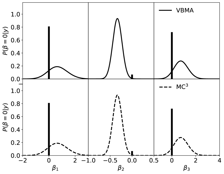
Figure 1: Posterior distributions for predictor slopes based on VBMA (first row) and MC³ (second row). Namely, $\beta_{1}$ corresponds to the percentage of males 14-24, $\beta_{2}$ to the probability of imprisonment, and $\beta_{3}$ to the mean years of schooling. The density is scaled so that the maximum of the density is equal to $\mathbb{P}(\beta\neq 0|\bm{d})$. The spike corresponds to to $\mathbb{P}(\beta=0|\bm{d})$.

Predictive Performance

Similar to Raftery et al. (1997), we asses the predictive ability of VBMA by randomly splitting the U.S. crime data into a training and a testing dataset. A 50-50 split was chosen here due to a relatively small size of the dataset. We subsequently re-run the VBMA (and MC³) using the training dataset. The predictive performance was measured through coverage of Bayesian predictive intervals (equal-tails) with the credibility level ranging from $10\%$ to $90\%$ with $10\%$ increments. A $(1-\alpha)\times 100\%$ prediction interval is a posterior credible interval within which a (predicted) observation falls with probability $(1-\alpha)$. An equal-tail interval is chosen so that the posterior probability of being below the interval is as likely as being above it (Gelman et al., 2013). Figure 2 shows the predictive coverage of the two methods plotted against each other with the diagonal dashed line indicating a perfect agreement between the methods. We can see that the coverages for the procedures match in general with small discrepancies at lower quantiles. Additionally, we compare the model averaging predictions with those obtained by the best models according to the adjusted $R^{2}$ and Mallows’ $C_{p}$ under both VBMA and MC³. Adjusted $R^{2}$ and Mallows’ $C_{p}$ are commonly used model selection and evaluation criteria in a regression setting. Adjusted $R^{2}$ measures quality of the model in terms of total variability explained, whereas Mallows’ $C_{p}$ estimates the size of the bias that is introduced into the predicted responses by having a model that is missing one or more important predictors (James et al., 2013). Both of these model selection strategies lead to $M_{3}$ as the best model. However, $M_{3}$ generally under-performed the model averaging and underestimated the declared coverage. We can see that by the general shift of the respected curve in comparison to the averaging results.

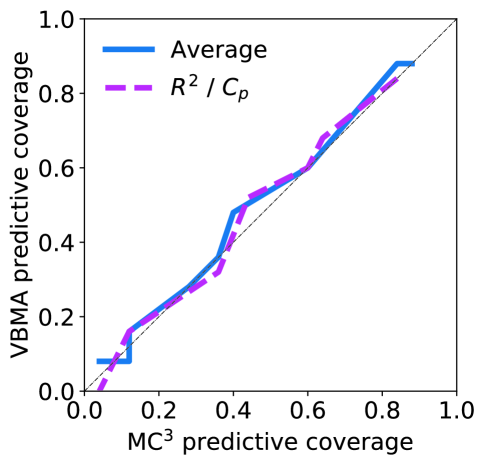
Figure 2: Comparison between coverages of Bayesian predictive interval (equal-tails) on a testing set of 22 observations. The horizontal axis corresponds to the predictive coverage of MC³ based intervals and the vertical axis to the coverage of VBMA. The diagonal line corresponds to the perfect agreement between the two methods.

3.2 Bayesian Logistic Regression

Unlike the standard linear regression, generalized linear models such as logistic regression exemplify the slew of challenges that one can encounter when implementing BMA. First, the evaluation of the evidence integral does not have an analytic form and the integration can be high-dimensional. Additionally, direct sampling from the BMA posterior through MC³ algorithm is not available. One therefore needs to approximate the evidence integral and consequently approximate the BMA posterior with MC samples from the mixture of the posteriors of each of the individual models.

Here we illustrate the utility of VBMA on the analysis of heart disease data (Dua and Graff, 2017) to asses the factors that contribute to the risk of heart attack. The models used are logistic regression models with logit link function of the form

$$\log\bigg{(}\frac{\mathbb{P}(y=1)}{\mathbb{P}(y=0)}\bigg{)}=\beta_{0}+\sum_{j=1}^{p}\beta_{j}x_{j},$$ (15)

where $y=1$ corresponds to subjects with higher chance of heart attack, and $y=0$ to those with a smaller chance of heart attack. In this example, we shall consider five predictors, namely $x_{1}$ is the serum cholestoral in g/dl, $x_{2}$ is their resting blood pressure on admission to the hospital, $x_{3}$ is the biological sex, $x_{4}$ is the age, and $x_{5}$ is the maximum hear rate achieved during examination. This gives the total of 32 candidate models. All the continuous variables were again log transformed and centered. For the parameters in each model (15), we use independent normal prior distributions.

3.2.1 Results

Table 2: The top eight logistic regression models of the heart rate data according to their posterior model probabilities. The star indicates the inclusion of predictor in the model and the model ID is provided for easier referencing. Comparison between the VBMA and the MC based averaging is shown.

	Inclusion						$p(M|\bm{d})$
Model	Intercept	$\bm{x_{1}}$	$\bm{x_{2}}$	$\bm{x_{3}}$	$\bm{x_{4}}$	$\bm{x_{5}}$	MC	VBMA
1	*	*	*	*		*	0.45	0.43
2	*	*	*	*	*	*	0.28	0.28
3	*	*		*	*	*	0.09	0.09
4	*	*		*		*	0.06	0.06
5	*		*	*	*	*	0.05	0.06
6	*		*	*		*	0.04	0.05
7	*			*	*	*	0.01	0.02
8	*			*		*	$<0.01$	$<0.01$

Table 2 shows the estimates of model posterior probabilities obtained with VBMA as compared to those computed using MC integration for the top 8 models. The VBMA results are based on a pre-training sequence of $500$ iterations with the model probabilities set to 1/32 and $100$ iterations of updating according to Algorithm 1. Ten MC samples from the variational distributions were used to estimate the ELBO gradient. The MC-based posterior model probabilities are based on $7.5\times 10^{5}$ samples. This large number of samples was necessary in order to achieve reasonable convergence. We again observe a close match of the VBMA model posteriors with the MC model posteriors.

Figure 3 shows the posterior distribution of regression coefficients based on the model average. The MCMC results were obtained with No-U-Turn sampler (Homan and Gelman, 2014) implemented in Python package for Bayesian statistical modeling PyMC3 (Salvatier et al., 2016). Analogically to the linear regression example, VBMA algorithm with reparametrization gradients captures the posterior distributions well including the parameter uncertainties. When it comes to the computation times, we start seeing the benefits of VBMA for non-conjugate models. The pre-training sequence took 3-4 seconds per model and the averaging of all 32 models took approximately 20 seconds on a mid-range laptop. On the other hand, the MC estimates of evidence integrals required 20 minutes per model, and 20-50 seconds was needed to obtain $3\times 10^{4}$ samples via No-U-Turn sampler.

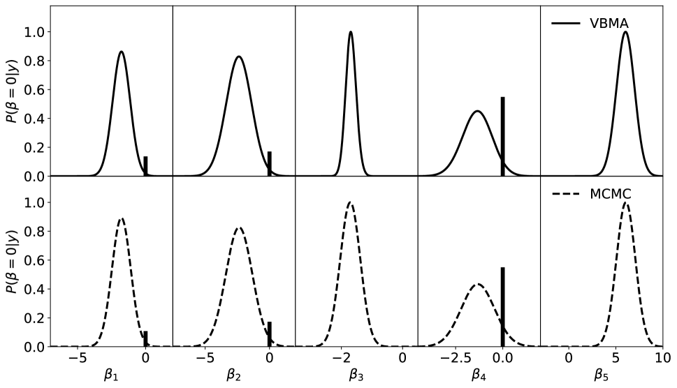
Figure 3: Posterior distributions for predictor slopes based on VBMA (first row) and MCMC (second row). Namely, $\beta_{1}$ corresponds to the serum cholestoral in g/dl, $\beta_{2}$ to the resting blood pressure on admission to the hospital, $\beta_{3}$ to the biological sex, $\beta_{4}$ to the age, and $\beta_{5}$ is the maximum hear rate achieved during examination. The density is scaled so that the maximum of the density is equal to $\mathbb{P}(\beta\neq 0|\bm{d})$. The spike corresponds to to $\mathbb{P}(\beta=0|\bm{d})$.

3.3 Bayesian Model Selection

Here, we demonstrate that the VBMA algorithm can be conveniently applied in the generalization of Bayesian hypotheses testing, that is, model selection with Bayes factors. Instead of averaging, suppose that we wish to compare the two Bayesian models,

$$M_{0}:\bm{d}\sim p(\bm{d}|\bm{\theta}_{0}),\bm{\theta}_{0}\sim p(\bm{\theta}_{0}),\hskip 14.22636ptM_{1}:\bm{d}\sim p(\bm{d}|\bm{\theta}_{1}),\bm{\theta}_{1}\sim p(\bm{\theta}_{1}),$$

where the definition of the parameter $\bm{\theta}$ may differ between models. Then, the Bayes factor $B_{01}$ in support of model $M_{0}$ is given by

$$B_{01}=\frac{p(\bm{d}|M_{0})}{p(\bm{d}|M_{1})}=\frac{p(M_{0}|\bm{d})p(M_{1})}{p(M_{1}|\bm{d})p(M_{0})},$$ (16)

where $p(M_{i}|\bm{d})$ for $i\in\{0,1\}$ is the model’s posterior probability defined in equation (2). The quantity $B_{01}$ is the ratio of the posterior odds of model $M_{0}$ to its prior odds and represents the information about the evidence provided by the data in favor of model $M_{0}$ as opposed to $M_{1}$ (Kass and Raftery, 1995). It should be clear from the definition of (16) that the Bayesian model selection suffers from exactly the same computational challenges as BMA. To this extent, VBMA directly approximates posterior probabilities of individual models and Bayes factors can be conveniently computed as a byproduct of the algorithm without the need of approximating the model evidence (3).

3.3.1 Linear and Logistic Regression Examples

To illustrate the Bayesian model selection via VBMA, we consider the following hypotheses for both linear and logistic regression examples above and compare the VBMA based results with their MC counterparts:

$$H_{0}:\beta_{1}=0,\hskip 14.22636ptH_{1}:\beta_{1}\neq 0.$$ (17)

For the linear regression case, this corresponds to comparing models $M_{1}$ and $M_{3}$. For the logistic regression example, we need to compare models $M_{5}$ and $M_{2}$. Table 3 presents the respective Bayes factor approximations. For both linear and logistic regression examples, VBMA approximations qualitatively agree with the MC based approximations. The results show that the U.S crime data favor the linear regression model with $\beta_{1}=0$, and the heart disease data favor logistic regression model with $\beta_{1}\neq 0$.

Table 3: Bayes factors obtained via VBMA approximation and MC methods. Models $M_{1}$ and $M_{3}$ are considered for the linear regression example and models $M_{5}$ and $M_{2}$ for the logistic regression example. Bayes factor larger than 1 indicates selection of the model with $\beta_{1}=0$ and vice versa.

	Bayes Factor
Example	MC	VBMA
Linear regression	2.43	3.00
Logistic regression	0.18	0.21

3.4 Nuclear Mass Predictions

As an illustration of VBMA in a scenario where application of standard MCMC-based inference is challenging in practice, we study the separation energies of atomic nuclei which were the subject of various recent machine learning applications (Gaussian process modeling) in the field of nuclear physics (Neufcourt et al., 2018, 2019, 2020b, 2020c). Namely, our focus is the two-neutron separation energy ($S_{2n}$) which is a fundamental property of atomic nucleus and is defined as the energy required to remove two neutrons from the nucleus. The $S_{2n}$ values can be obtained through a nuclear mass difference. The knowledge of separation energies determines the limits of nuclear existence and predictions of these quantities can help guide the experimental research at future rare isotope facilities.

In this example, we shall consider 6 state-of-the-art nuclear mass models based on the nuclear density functional theory (DFT) (Nazarewicz, 2016): the Skyrme energy density functionals SkM^∗ (Bartel et al., 1982), SkP (Dobaczewski et al., 1984), SLy4 (Chabanat et al., 1995), SV-min (Klüpfel et al., 2009), UNEDF0 Kortelainen et al. (2010), and UNEDF1 (Kortelainen et al., 2012). These are global nuclear mass models, because the are capable of reliably describing the whole nuclear chart. Our analysis closely follows that of Neufcourt et al. (2020c), where we consider the statistical model for the differences $y_{i}=S_{2n}^{exp}(\bm{x}_{i})-S_{2n}^{th}(\bm{x}_{i})$ between the observed experimental data and the predictions given by the theoretical models of the form

$$y_{i}=f(\bm{x}_{i})+\sigma\epsilon_{i},$$ (18)

where $\bm{x}_{i}=(Z_{i},N_{i})$ corresponds to the the proton number $Z_{i}$ and the neutron number $N_{i}$ of a nucleus. The function $f(\cdot)$ represents the systematic discrepancy between the underlying physical process and the theoretical mass model. The quantity $\sigma\epsilon_{i}$ is the scaled experimental error which is assumed to be i.i.d. normal with mean zero. For the systematic discrepancy, Neufcourt et al. (2020c) take a Gaussian process (GP) on the two dimensional space $x=(Z,N)$:

$$f(\bm{x})\sim\mathcal{GP}(\beta,k(\bm{x},\bm{x}^{\prime})),$$ (19)

where $\beta$ is the constant mean and $k$ is the squared exponential covariance function characterized by the scale $\eta$ and characteristic correlation ranges $\nu_{Z}$ and $\nu_{N}$:

$$k(\bm{x},\bm{x}^{\prime})=\eta^{2}e^{-\frac{(Z-Z^{\prime})^{2}}{2\nu_{Z}^{2}}-\frac{(N-N^{\prime})^{2}}{2\nu_{N}^{2}}}.$$ (20)

The GP with covariance (20) is a sensible nonparametric model for the systematic discrepancy as it is expected to be relatively smooth and stationary (Neufcourt et al., 2020a). Since neither of the six Skyrme energy functionals a-priory stands out on the full nuclear domain, using BMA for averaging or model selection is a logical approach here that will allow for predictions with realistically quantified uncertainties.

As the experimental observations, we take the most recent measured values of two-neutron separation energies from the AME2003 dataset (Audi et al., 2003) as training data ($n=1029$) and keep all additional data tabulated in AME2016 (Wang et al., 2017) for a testing dataset $(n=120)$. The domains of these datasets are depicted in Figure 4. Note that we use both even-even (meaning both $Z$ and $N$ are even) and odd-even nuclei jointly for the training to fully account for the correlations between systematic discrepancies unlike Neufcourt et al. (2020c) who fitted independent GPs on the two domains separately to make the computations manageable. Using the proposed VBMA approach, we are able to do computations in matter of minutes which would take dozens of hours using the standard MCMC approximation.

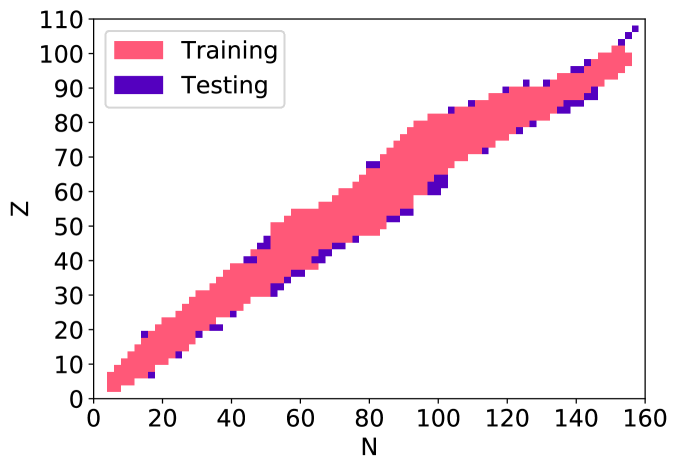
Figure 4: The nuclear chart of even-even and odd-even nuclei divided into the training and testing datasets for the GP modeling of the residuals of two-neutron separation energies $S_{2n}$. $Z$ corresponds to the proton number and $N$ is the neutron number.

3.5 Results

The performance of VBMA in averaging of the GP enhanced nuclear mass models was compared with BMA based on the posterior approximation by No-U-Turn sampler and the MC estimates of evidence integrals. Similarly to the previous examples, the VBMA results are based on a pre-training sequence of $300$ iterations with the model probabilities set to 1/6. This pre-training sequence lead to the selection of UNEDF1 ($p(M|\bm{d})=1$) with stable ELBOs and so no further training was needed. Ten MC samples from the variational distributions were used to estimate the reparametrization gradient gradient. The resulting root-mean-square error (RMSE) on the testing dataset of 120 nuclei was 0.406 MeV as compared to the RMSE of 0.419 MeV given by the MCMC approximation. These RMSE values are consistent with those obtained by Neufcourt et al. (2020c). The MCMC results are based on $2\times 10^{4}$ posterior samples ($10^{4}$ burn-in) and the MC posterior model probabilities are based on $2\times 10^{5}$ samples which also lead to the selection of UNEDF1.

The MCMC implementation proved to be significantly more time consuming. It required 15-20 hours per model to generate the posterior samples and about six hours for the MC integration. On the other hand, the variational approach required between 20 to 25 minutes per model which clearly demonstrates the utility of VBMA in more complex modeling scenarios. The fidelity of Bayesian predictive intervals was equivalent between the VBMA and MCMC similarly to the linear regression example. We refer the reader to the Supplement for additional results containing the study of predictive coverage.

4 Discussion

We presented a VBI approach to BMA that avoids some of the practical challenges that burdens the standard MCMC based approaches to approximate the BMA posterior, especially numerical evaluation of the evidence integral and long sampling times of MCMC sampler. The fidelity of the method was demonstrated on a series of pedagogical examples including the averaging of linear and logistic regression models and Bayesian model selection via Bayes factors. To fully showcase the computational benefits of VBMA, we applied our methodology to nuclear mass models with GP model for systematic discrepancies. The observed speed-up in the case of GP modeling was at least fifty-fold compared to the standard MCMC approaches.

The proposed procedure is “black box” in the sense that it can be readily applied to wide range of models with minimal additional derivations needed. For instance, VBMA can be conveniently applied to nonconjugate models including generalized linear models, Bayesian neural networks, and Deep latent Gaussian models (Blei et al., 2017).

Additionally, VBMA is a general VBI algorithm and the presented implementation with the Adam learning rate and the mean-field variational family is just one of many implementations. One can consider any adaptive learning rate and other variational family available in the literature. VBMA can also be simply modified for greater scalability in the scenarios with complex machine learning models that need to be fitted to massive datasets. First, one can subsample from the data to construct computationally cheap noisy estimates of ELBO gradients. Secondly, the nature of VBMA allows for immediate parallelization across the models. To achieve a faster convergence of the algorithm, VBMA can be augmented with Rao-Blackwellizaiton (Casella and Robert, 1996), control variates (Ross, 2006), and importance sampling Ruiz et al. (2016) to even further reduce the variance of noisy gradient estimators.

Of course, the use of VBI comes at a cost and one cannot avoid the general pitfalls of variational methods. Using mean-field families can lead to posterior distributions with underestimated uncertainties in cases of highly correlated parameters. One can improve the fidelity of posteriors by using more complex variational family that does not assume independence of unknown parameters (Blei et al., 2017; Wang and Blei, 2018). The choice of adaptive learning rate can be sometimes challenging in practice, and one may observe significant differences among the adaptive learning rates, and a careful sensitivity analysis must be performed. For the models considered in this work, we do not observe significant differences between the RMSprop and the Adam (see the Supplement). The reparametrization gradient used in Algorithm 1 works only for differentiable models with no discrete variables. One can use the score gradient (Ranganath et al., 2014) for models with discrete variables which is also black box in nature, however, the variance of the gradient estimates is larger than that of reparametrization gradients. Lastly, the computational overhead of VBMA for simple models (such as linear regression) can be too high to achieve any meaningful advantage, however, the use of VBMA in complex models can lead to significant computational gains.

Acknowledgments

The authors thank the reviewers, the Associate Editor, and the Editor for their helpful comments and ideas. This work was supported in part through computational resources and services provided by the Institute for Cyber-Enabled Research at Michigan State University.

Funding

The research is partially supported by the National Science Foundation funding DMS-1952856 and OAC-2004601.

Appendix A Parametrization of Variational Families

A.1 Normal Variational Family

Let us consider a real valued parameter $\theta$ with normal variation family $q(\theta|\mu,\sigma^{2})$ parametrized by the mean $\mu$ and variance $\sigma^{2}$. Under the transformation (13), we get the following expressions for the log likelihood of the variational distribution

$$\log q(\theta|\mu,\lambda_{\sigma})=-\frac{1}{2}\log[\log(e^{\lambda_{\sigma}}+1)]-\frac{1}{2}\log 2\pi-\frac{1}{2}\frac{(\theta-\mu)^{2}}{\log(e^{\lambda_{\sigma}}+1)}.$$ (21)

The reparametrization gradient is then obtained with $z\sim\text{Normal}(0,1)$ so that

$$\theta=t(z,(\mu,\lambda_{\sigma}))=z\times\sqrt{\log(e^{\lambda_{\sigma}}+1)}+\mu.$$

A.2 Log-normal Variational Family

For a positive-valued parameters, we shall consider a log-normal variational family $q(\theta|m,\tau^{2})$ parametrized by the mean $m$ and variance $\tau^{2}$:

$$\log q(\theta|m,\lambda_{\tau})=-\log\theta-\frac{1}{2}\log[\log(e^{\lambda_{\tau}}+1)]-\frac{1}{2}\log 2\pi-\frac{1}{2}\frac{(\log\theta-\mu)^{2}}{\log(e^{\lambda_{\tau}}+1)}$$

The reparametrization gradient is then obtained with $z\sim\text{Normal}(0,1)$ so that

$$\theta=t(z,(\mu,\lambda_{\tau}))=e^{z\times\sqrt{\log(e^{\lambda_{\tau}}+1)}+\mu}.$$

References

- Ambrogioni et al. (2021) Ambrogioni, L., K. Lin, E. Fertig, S. Vikram, M. Hinne, D. Moore, and M. van Gerven (2021, 13–15 Apr). Automatic structured variational inference. In A. Banerjee and K. Fukumizu (Eds.), Proceedings of The 24th International Conference on Artificial Intelligence and Statistics, Volume 130 of Proceedings of Machine Learning Research, pp. 676–684. PMLR.
- Ardia et al. (2012) Ardia, D., N. Baştürk, L. Hoogerheide, and H. K. van Dijk (2012). A comparative study of monte carlo methods for efficient evaluation of marginal likelihood. Computational Statistics and Data Analysis 56(11), 3398–3414. 1st issue of the Annals of Computational and Financial Econometrics Sixth Special Issue on Computational Econometrics.
- Audi et al. (2003) Audi, G., A. Wapstra, and C. Thibault (2003). The AME2003 atomic mass evaluation: (ii). tables, graphs and references. Nuclear Physics A 729, 337–676.
- Balasubramanian et al. (2014) Balasubramanian, J. B., S. Visweswaran, G. F. Cooper, and V. Gopalakrishnan (2014). Selective model averaging with Bayesian rule learning for predictive biomedicine. AMIA Joint Summits on Translational Science proceedings AMIA Summit on Translational Science 2014, 17–22.
- Bartel et al. (1982) Bartel, J., P. Quentin, M. Brack, C. Guet, and H.-B. Håkansson (1982). Towards a better parametrisation of Skyrme-like effective forces: a critical study of the SkM force. Nuclear Physics A 386(1), 79–100.
- Bernardo and Smith (1994) Bernardo, J. M. and A. F. M. Smith (1994). Reference analysis, Chapter Inference. Wiley.
- Bhattacharya and Maiti (2021) Bhattacharya, S. and T. Maiti (2021). Statistical foundation of variational bayes neural networks. Neural Networks 137, 151–173.
- Blei et al. (2017) Blei, D. M., A. Kucukelbir, and J. D. McAuliffe (2017). Variational inference: A review for statisticians. Journal of the American Statistical Association 112(518), 859–877.
- Bottou et al. (1997) Bottou, L., Y. Le Cun, and Y. Bengio (1997). Global training of document processing systems using graph transformer networks. In Proceedings of Computer Vision and Pattern Recognition (CVPR), pp. 489–493. IEEE.
- Casella and Robert (1996) Casella, G. and C. P. Robert (1996). Rao-blackwellisation of sampling schemes. Biometrika 83(1), 81–94.
- Chabanat et al. (1995) Chabanat, E., P. Bonche, P. Haensel, J. Meyer, and R. Schaeffer (1995). New Skyrme effective forces for supernovae and neutron rich nuclei. Physica Scr. 1995(T56), 231.
- Clarke (2003) Clarke, B. (2003, 11). Comparing bayes model averaging and stacking when model approximation error cannot be ignored. The Journal of Machine Learning Research 4, 683–712.
- Clyde and Iversen (2013) Clyde, M. and E. Iversen (2013, 01). Bayesian Model Averaging in the M-Open Framework, pp. 484–498.
- Clyde et al. (2011) Clyde, M. A., J. Ghosh, and M. L. Littman (2011). Bayesian adaptive sampling for variable selection and model averaging. Journal of Computational and Graphical Statistics 20, 80–101.
- Dobaczewski et al. (1984) Dobaczewski, J., H. Flocard, and J. Treiner (1984). Hartree-Fock-Bogolyubov description of nuclei near the neutron-drip line. Nucl. Phys. A 422(1), 103–139.
- Dua and Graff (2017) Dua, D. and C. Graff (2017). UCI machine learning repository.
- Duchi et al. (2011) Duchi, J., E. Hazan, and Y. Singer (2011). Adaptive subgradient methods for online learning and stochastic optimization. The Journal of Machine Learning Research 12, 2121–2159.
- Feroz et al. (2009) Feroz, F., M. P. Hobson, and M. Bridges (2009). Multinest: an efficient and robust bayesian inference tool for cosmology and particle physics. Monthly Notices of the Royal Astronomical Society 398, 1601–1614.
- Fortunato et al. (2017) Fortunato, M., C. Blundell, and O. Vinyals (2017). Bayesian recurrent neural networks. arXiv preprint arXiv: 1704.02798.
- Fragoso et al. (2018) Fragoso, T. M., W. Bertoli, and F. Louzada (2018). Bayesian model averaging: A systematic review and conceptual classification. International Statistical Review 86, 1–28.
- Friel and Pettitt (2008) Friel, N. and A. N. Pettitt (2008). Marginal likelihood estimation via power posteriors. Journal of the Royal Statistical Society: Series B (Statistical Methodology) 70(3), 589–607.
- Friel and Wyse (2012) Friel, N. and J. Wyse (2012). Estimating the evidence – a review. Statistica Neerlandica 66(3), 288–308.
- Gelman et al. (2013) Gelman, A., J. Carlin, H. Stern, D. Dunson, A. Vehtari, and D. Rubin (2013). Bayesian Data Analysis (Third ed.). CRC Pres.
- Geweke (1999) Geweke, J. (1999). Using simulation methods for Bayesian econometric models: inference, development, and communication. Econometric Reviews 18, 1–73.
- Hernández et al. (2018) Hernández, B., A. E. Raftery, S. R. Pennington, and A. C. Parnell (2018). Bayesian additive regression trees using Bayesian model averaging. Statistics and Computing 28, 869–890.
- Hoeting et al. (1999) Hoeting, J. A., D. Madigan, A. E. Raftery, and C. T. Volinsky (1999). Bayesian model averaging: A tutorial. Statistical Science 14, 382–401.
- Hoffman and Blei (2015) Hoffman, M. and D. Blei (2015, 09–12 May). Stochastic structured variational inference. In Proceedings of the Eighteenth International Conference on Artificial Intelligence and Statistics, Volume 38, San Diego, CA, pp. 361–369. PMLR.
- Homan and Gelman (2014) Homan, M. D. and A. Gelman (2014). The No-U-Turn Sampler: Adaptively setting path lengths in Hamiltonian Monte Carlo. Journal of Machine Learning Research 15, 1351–1381.
- Hooten and Hobbs (2015) Hooten, M. B. and N. T. Hobbs (2015). A guide to Bayesian model selection for ecologists. Ecological Monographs 85, 3–28.
- James et al. (2013) James, G., D. Witten, T. Hastie, and R. Tibshirani (2013). An Introduction to Statistical Learning: with Applications in R. New York, NY: Springer New York.
- Jaureguiberry et al. (2014) Jaureguiberry, X., E. Vincent, and G. Richard (2014). Variational bayesian model averaging for audio source separation. In 2014 IEEE Workshop on Statistical Signal Processing (SSP), pp. 33–36.
- Jordan et al. (1999) Jordan, M. I., Z. Ghahramani, T. S. Jaakkola, and L. K. Saul (1999). An introduction to variational methods for graphical models. Machine Learning 37, 183–233.
- Kass and Raftery (1995) Kass, R. E. and A. E. Raftery (1995). Bayes factors. Journal of the American Statistical Association 90, 773–795.
- Kejzlar et al. (2020) Kejzlar, V., L. Neufcourt, W. Nazarewicz, and P.-G. Reinhard (2020, jul). Statistical aspects of nuclear mass models. Journal of Physics G: Nuclear and Particle Physics 47(9), 094001.
- Kingma and Ba (2014) Kingma, D. and J. Ba (2014, 12). Adam: A method for stochastic optimization. International Conference on Learning Representations.
- Kingma et al. (2016) Kingma, D. P., T. Salimans, R. Jozefowicz, X. Chen, I. Sutskever, and M. Welling (2016). Improved variational inference with inverse autoregressive flow. In D. Lee, M. Sugiyama, U. Luxburg, I. Guyon, and R. Garnett (Eds.), Advances in Neural Information Processing Systems, Volume 29. Curran Associates, Inc.
- Klüpfel et al. (2009) Klüpfel, P., P.-G. Reinhard, T. J. Bürvenich, and J. A. Maruhn (2009, Mar). Variations on a theme by Skyrme: A systematic study of adjustments of model parameters. Phys. Rev. C 79(3), 034310.
- Kobyzev et al. (2021) Kobyzev, I., S. J. Prince, and M. A. Brubaker (2021, Nov). Normalizing flows: An introduction and review of current methods. IEEE Transactions on Pattern Analysis and Machine Intelligence 43(11), 3964–3979.
- Kortelainen et al. (2010) Kortelainen, M., T. Lesinski, J. J. Moré, W. Nazarewicz, J. Sarich, N. Schunck, M. V. Stoitsov, and S. M. Wild (2010). Nuclear energy density optimization. Physical Review C 82(2), 024313.
- Kortelainen et al. (2012) Kortelainen, M., J. McDonnell, W. Nazarewicz, P.-G. Reinhard, J. Sarich, N. Schunck, M. V. Stoitsov, and S. M. Wild (2012). Nuclear energy density optimization: large deformations. Physical Review C 85, 024304.
- Kucukelbir et al. (2017) Kucukelbir, A., D. Tran, R. Ranganath, A. Gelman, and D. M. Blei (2017). Automatic differentiation variational inference. Journal of Machine Learning Research 18(14), 1–45.
- Latouche and Robin (2016) Latouche, P. and S. S. Robin (2016). Variational Bayes model averaging for graphon functions and motif frequencies inference in W-graph models. Statistics and Computing 26(6), 1173 – 1185.
- Leamer (1978) Leamer, E. E. (1978). Specification Searches: Ad Hoc Inference with Nonexperimental Data. Wiley.
- Lenk (2009) Lenk, P. (2009). Simulation pseudo-bias correction to the harmonic mean estimator of integrated likelihoods. Journal of Computational and Graphical Statistics 18(4), 941–960.
- Madigan et al. (1995) Madigan, D., J. Gavrin, and A. E. Raftery (1995). Eliciting prior information to enhance the predictive performance of bayesian graphical models. Communications in Statistics - Theory and Methods 24(9), 2271–2292.
- Masegosa (2020) Masegosa, A. (2020). Learning under model misspecification: Applications to variational and ensemble methods. In H. Larochelle, M. Ranzato, R. Hadsell, M. F. Balcan, and H. Lin (Eds.), Advances in Neural Information Processing Systems, Volume 33, pp. 5479–5491. Curran Associates, Inc.
- Mukhopadhyay and Dunson (2020) Mukhopadhyay, M. and D. B. Dunson (2020). Targeted random projection for prediction from high-dimensional features. Journal of the American Statistical Association 115(532), 1998–2010.
- Nazarewicz (2016) Nazarewicz, W. (2016). Challenges in nuclear structure theory. Journal of Physics G: Nuclear and Particle Physics 43, 044002.
- Neal (2001) Neal, R. (2001, 01). Annealed importance sampling. Statistics and Computing 11.
- Neufcourt et al. (2020a) Neufcourt, L., Y. Cao, S. Giuliani, W. Nazarewicz, E. Olsen, and O. B. Tarasov (2020a, Jan). Beyond the proton drip line: Bayesian analysis of proton-emitting nuclei. Physical Review C 101, 014319.
- Neufcourt et al. (2020b) Neufcourt, L., Y. Cao, S. Giuliani, W. Nazarewicz, E. Olsen, and O. B. Tarasov (2020b, Jan). Beyond the proton drip line: Bayesian analysis of proton-emitting nuclei. Phys. Rev. C 101, 014319.
- Neufcourt et al. (2020c) Neufcourt, L., Y. Cao, S. A. Giuliani, W. Nazarewicz, E. Olsen, and O. B. Tarasov (2020c, Apr). Quantified limits of the nuclear landscape. Phys. Rev. C 101, 044307.
- Neufcourt et al. (2019) Neufcourt, L., Y. Cao, W. Nazarewicz, E. Olsen, and F. Viens (2019, Feb). Neutron drip line in the Ca region from Bayesian Model Averaging. Physical Review Letters 122, 062502.
- Neufcourt et al. (2018) Neufcourt, L., Y. Cao, W. Nazarewicz, and F. Viens (2018). Bayesian approach to model-based extrapolation of nuclear observables. Physical Review C 98, 034318.
- Pajor (2017) Pajor, A. (2017). Estimating the Marginal Likelihood Using the Arithmetic Mean Identity. Bayesian Analysis 12(1), 261 – 287.
- Papamakarios et al. (2021) Papamakarios, G., E. Nalisnick, D. J. Rezende, S. Mohamed, and B. Lakshminarayanan (2021). Normalizing flows for probabilistic modeling and inference. Journal of Machine Learning Research 22(57), 1–64.
- Papamakarios et al. (2017) Papamakarios, G., T. Pavlakou, and I. Murray (2017). Masked autoregressive flow for density estimation. In I. Guyon, U. V. Luxburg, S. Bengio, H. Wallach, R. Fergus, S. Vishwanathan, and R. Garnett (Eds.), Advances in Neural Information Processing Systems, Volume 30. Curran Associates, Inc.
- Paszke et al. (2019) Paszke, A., S. Gross, F. Massa, A. Lerer, J. Bradbury, G. Chanan, T. Killeen, Z. Lin, N. Gimelshein, L. Antiga, A. Desmaison, A. Kopf, E. Yang, Z. DeVito, M. Raison, A. Tejani, S. Chilamkurthy, B. Steiner, L. Fang, J. Bai, and S. Chintala (2019). Pytorch: An imperative style, high-performance deep learning library. In Advances in Neural Information Processing Systems 32, pp. 8024–8035. Curran Associates, Inc.
- Peterson and Anderson (1987) Peterson, C. and J. R. Anderson (1987). A mean field theory learning algorithm for neural networks. Complex Systems 1, 995–1019.
- Phillips et al. (2021) Phillips, D. R., R. J. Furnstahl, U. Heinz, T. Maiti, W. Nazarewicz, F. M. Nunes, M. Plumlee, M. T. Pratola, S. Pratt, F. G. Viens, and S. M. Wild (2021, 5). Get on the band wagon: a bayesian framework for quantifying model uncertainties in nuclear dynamics. Journal of Physics. G, Nuclear and Particle Physics 48(7).
- Raftery et al. (1997) Raftery, A. E., D. Madigan, and J. A. Hoeting (1997). Bayesian model averaging for linear regression models. Journal of the American Statistical Association 92(437), 179–191.
- Raftery et al. (2007) Raftery, A. E., M. A. Newton, J. M. Satagopa, and P. N. Krivitsk (2007). Estimating the integrated likelihood via posterior simulation using the harmonic mean identity. In Bayesian Statistics 8, pp. 1–45. Oxford University Press.
- Ranganath et al. (2014) Ranganath, R., S. Gerrish, and D. Blei (2014). Black box variational inference. In Proceedings of the Seventeenth International Conference on Artificial Intelligence and Statistics, Volume 33 of Proceedings of Machine Learning Research, pp. 814–822. PMLR.
- Ranganath et al. (2016) Ranganath, R., D. Tran, and D. M. Blei (2016). Hierarchical variational models. In Proceedings of the 33rd International Conference on International Conference on Machine Learning – Volume 48, ICML’16, pp. 2568–2577. JMLR.
- Rezende and Mohamed (2015) Rezende, D. and S. Mohamed (2015, 07–09 Jul). Variational inference with normalizing flows. In F. Bach and D. Blei (Eds.), Proceedings of the 32nd International Conference on Machine Learning, Volume 37 of Proceedings of Machine Learning Research, Lille, France, pp. 1530–1538. PMLR.
- Robbins and Monro (1951) Robbins, H. and S. Monro (1951, 09). A stochastic approximation method. Annals of Mathematical Statistics 22(3), 400–407.
- Ross (2006) Ross, S. M. (2006). Simulation (Fourth ed.). Orlando, FL: Academic Press, Inc.
- Ruiz et al. (2016) Ruiz, F. J. R., M. K. Titsias, and D. M. Blei (2016). Overdispersed black-box variational inference. In Proceedings of the Thirty-Second Conference on Uncertainty in Artificial Intelligence, UAI’16, Arlington, Virginia, USA, pp. 647–656. AUAI Press.
- Salvatier et al. (2016) Salvatier, J., T. V. Wiecki, and C. Fonnesbeck (2016). Probabilistic programming in python using pymc3. PeerJ Computer Science 2, e55.
- Schorning et al. (2016) Schorning, K., B. Bornkamp, F. Bretz, and H. Dette (2016). Model selection versus model averaging in dose finding studies. Statistics in Medicine 35, 4021–4040.
- Shazeer and Stern (2018) Shazeer, N. and M. Stern (2018, 10–15 Jul). Adafactor: Adaptive learning rates with sublinear memory cost. In J. Dy and A. Krause (Eds.), Proceedings of the 35th International Conference on Machine Learning, Volume 80 of Proceedings of Machine Learning Research, pp. 4596–4604. PMLR.
- Silvestro et al. (2014) Silvestro, D., J. Schnitzler, L. H. Liow, A. Antonelli, and N. Salamin (2014). Bayesian estimation of speciation and extinction from incomplete fossil occurrence data. Systematic Biology 63, 349–367.
- Skilling (2006) Skilling, J. (2006). Nested sampling for general bayesian computation. Bayesian Analysis 1(4), 833–860.
- Steel (2020) Steel, M. F. J. (2020, September). Model averaging and its use in economics. Journal of Economic Literature 58(3), 644–719.
- Tieleman and Hinton (2012) Tieleman, T. and G. Hinton (2012). Lecture 6.5—RmsProp: Divide the gradient by a running average of its recent magnitude. COURSERA: Neural Networks for Machine Learning.
- Titsias and Lázaro-Gredilla (2014) Titsias, M. and M. Lázaro-Gredilla (2014, 22–24 Jun). Doubly stochastic variational bayes for non-conjugate inference. In E. P. Xing and T. Jebara (Eds.), Proceedings of the 31st International Conference on Machine Learning, Volume 32 of Proceedings of Machine Learning Research, Bejing, China, pp. 1971–1979. PMLR.
- Tran et al. (2015) Tran, D., D. M. Blei, and E. M. Airoldi (2015). Copula variational inference. In Proceedings of the 28th International Conference on Neural Information Processing Systems - Volume 2, NeurIPS’15, Cambridge, MA, pp. 3564–3572. MIT Press.
- Tran et al. (2017) Tran, D., R. Ranganath, and D. M. Blei (2017). Hierarchical implicit models and likelihood-free variational inference. In Proceedings of the 31st International Conference on Neural Information Processing Systems, NeurIPS’17, pp. 5529–5539.
- Vandaele (1978) Vandaele, W. (1978). Participation in illegitimate activities-ehrlich revisited (from deterrence and incapacitation-estimating the effects of criminal sanctions on crime rates, p 270-335, 1978, alfred blumstein et al, ed.-see ncj-44669).
- Vaswani et al. (2017) Vaswani, A., N. Shazeer, N. Parmar, J. Uszkoreit, L. Jones, A. N. Gomez, L. u. Kaiser, and I. Polosukhin (2017). Attention is all you need. In I. Guyon, U. V. Luxburg, S. Bengio, H. Wallach, R. Fergus, S. Vishwanathan, and R. Garnett (Eds.), Advances in Neural Information Processing Systems, Volume 30. Curran Associates, Inc.
- Wainwright and Jordan (2008) Wainwright, M. J. and M. I. Jordan (2008). Graphical models, exponential families, and variational inference. Foundations and Trends® in Machine Learning 1(1–2), 1–305.
- Wang et al. (2017) Wang, M., G. Audi, F. G. Kondev, W. J. Huang, S. Naimi, and X. Xu (2017). The AME2016 atomic mass evaluation (II). tables, graphs and references. Chinese Physics C 41, 030003.
- Wang and Blei (2018) Wang, Y. and D. M. Blei (2018). Frequentist consistency of variational Bayes. Journal of the American Statistical Association 0(0), 1–15.
- Wei et al. (2011) Wei, W., S. Visweswaran, and G. F. Cooper (2011). The application of naive Bayes model averaging to predict Alzheimer’s disease from genome-wide data. Journal of the American Medical Informatics Association 18, 370–375.
- Weilbach et al. (2020) Weilbach, C., B. Beronov, F. Wood, and W. Harvey (2020, 26–28 Aug). Structured conditional continuous normalizing flows for efficient amortized inference in graphical models. In S. Chiappa and R. Calandra (Eds.), Proceedings of the Twenty Third International Conference on Artificial Intelligence and Statistics, Volume 108 of Proceedings of Machine Learning Research, pp. 4441–4451. PMLR.
- Wen (2015) Wen, X. (2015). Bayesian model comparison in genetic association analysis: linear mixed modeling and SNP set testing. Biostatistics 16, 701–712.
- Zeiler (2012) Zeiler, M. D. (2012). Adadelta: An adaptive learning rate method. ArXiv 1212.5701.
- Zellner (1986) Zellner, A. (1986). On assessing prior distributions and bayesian regression analysis with g prior distributions. Bayesian Inference and Decision Techniques: Essays in Honor of Brune de Finetti, 233–243.
- Zhang and Gao (2020) Zhang, F. and C. Gao (2020). Convergence rates of variational posterior distributions. The Annals of Statistics 48(4), 2180 – 2207.