An inverse random source problem for the biharmonic wave equation

Peijun Li Department of Mathematics, Purdue University, West Lafayette, Indiana 47907, USA lipeijun@math.purdue.edu  and  Xu Wang Department of Mathematics, Purdue University, West Lafayette, Indiana 47907, USA wang4191@purdue.edu
Abstract.

This paper is concerned with an inverse source problem for the stochastic biharmonic operator wave equation. The driven source is assumed to be a microlocally isotropic Gaussian random field with its covariance operator being a classical pseudo-differential operator. The well-posedness of the direct problem is examined in the distribution sense and the regularity of the solution is discussed for the given rough source. For the inverse problem, the strength of the random source, involved in the principal symbol of its covariance operator, is shown to be uniquely determined by a single realization of the magnitude of the wave field averaged over the frequency band with probability one. Numerical experiments are presented to illustrate the validity and effectiveness of the proposed method for the case that the random source is the white noise.

Key words and phrases:
inverse random source problem, biharmonic operator, Gaussian random fields, stochastic differential equations, pseudo-differential operator, principal symbol
2010 Mathematics Subject Classification:
35R30, 35R60, 65M32
The research is supported in by part the NSF grant DMS-1912704.

1. Introduction

As one of the important research subjects in inverse scattering theory, inverse source problems for wave propagation have diverse scientific and industrial applications such as antenna design and synthesis, medical imaging [11]. They have continuously attracted much attention from many researchers. We refer to [5] and the references cited therein for some recent advances on this topic. Meanwhile, the study on boundary value problems for higher-order elliptic operators has generated sustained interest in the mathematics community [7]. The biharmonic operator, which may arise from the modeling of elasticity for example, appears to be a natural candidate for such a study [23, 24, 25]. Compared with inverse problems involving the second order differential operators, the inverse problems for the biharmonic operator are much less studied. The reason is not only the increase of the order which leads to the failure of the methods developed for the second order equations, but also the properties of the solutions for the higher order equations are more sophisticated. Some of the inverse boundary value problems for bi- and poly-harmonic operators can be found in [8, 12, 13, 21, 26, 27, 28].

In practice, there are many uncertainties caused by the unpredictability of the surrounding environment, incomplete knowledge of the studied system, fine-scale spatial or temporal variations, etc., which cannot be neglected during analysis or simulation. To take account of uncertainties, it would be reasonable and important to introduce random parameters to the mathematical modeling. Stochastic inverse problems refer to as inverse problems that involve randomness. Compared to their deterministic counterparts, stochastic inverse problems are more difficult due to two extra challenges: the random parameter is sometimes too rough to exist point-wisely and can only be interpreted as a distribution; the statistics such as the average and variance of the random parameter are required to be reconstructed. New methodology needs to be developed not only for the inverse problems but also for the corresponding direct problems in stochastic settings.

In this work, we consider an inverse source problem for the stochastic biharmonic wave equation

Δ2uk4u=find,superscriptΔ2𝑢superscript𝑘4𝑢𝑓insuperscript𝑑\Delta^{2}u-k^{4}u=f\quad\text{in}~{}\mathbb{R}^{d}, (1.1)

where d=2𝑑2d=2 or 333 and k>0𝑘0k>0 is the wavenumber. The wave field u𝑢u and its Laplacian ΔuΔ𝑢\Delta u are required to satisfy the Sommerfeld radiation condition

limrrd12(ruiku)=limrrd12(rΔuikΔu)=0,r=|x|.formulae-sequencesubscript𝑟superscript𝑟𝑑12subscript𝑟𝑢i𝑘𝑢subscript𝑟superscript𝑟𝑑12subscript𝑟Δ𝑢i𝑘Δ𝑢0𝑟𝑥\lim_{r\to\infty}r^{\frac{d-1}{2}}\left(\partial_{r}u-{\rm i}ku\right)=\lim_{r\to\infty}r^{\frac{d-1}{2}}\left(\partial_{r}\Delta u-{\rm i}k\Delta u\right)=0,\quad r=|x|. (1.2)

The source f𝑓f is assumed to be a microlocally isotropic Gaussian random field of order m𝑚-m (cf. Definition 1) such that its covariance operator is a classical pseudo-differential operator with principal symbol μ(x)|ξ|m𝜇𝑥superscript𝜉𝑚\mu(x)|\xi|^{-m}, where μ𝜇\mu is called the strength of the random source f𝑓f. The microlocally isotropic Gaussian random field can be viewed as one of the generalized fractional Gaussian random fields (cf. [18]), which cover a wide class of frequently studied Gaussian random fields, such as the white noise with m=0𝑚0m=0 and translations of the classical fractional Brownian motions with m(d,d+1)𝑚𝑑𝑑1m\in(d,d+1). In particular, if md𝑚𝑑m\leq d, the random field f𝑓f is too rough to exist point-wisely, and should be interpreted as a distribution.

For the white noise case with m=0𝑚0m=0, the random source can be equivalently rewritten as f=μW˙𝑓𝜇˙𝑊f=\sqrt{\mu}\dot{W}, where W˙˙𝑊\dot{W} denotes the white noise. Then the biharmonic wave equation (1.1) is interpreted as a stochastic partial differential equation driven by an additive white noise. The Itô isometry can be used in this case to derive the recovery formula for the strength μ𝜇\mu. We refer to [2, 4] and [3] for the inverse random source problem of the acoustic and elastic wave equations, respectively, where the strength μ𝜇\mu is shown to be uniquely determined by the variance of the wave field at multiple frequencies.

As a generalized Gaussian random field, the microlocally isotropic Gaussian random field with a general m𝑚m is studied in recent years (cf. [6, 9, 16, 18]) to handle a larger class of Gaussian random fields whose increments are not independent if m0𝑚0m\neq 0 and hence the Itô isometry is not available. For the case m[d,d+12)𝑚𝑑𝑑12m\in[d,d+\frac{1}{2}), by using the microlocal analysis of the Fourier integral operators, it was shown in [16] for both the acoustic and elastic wave equations that the strength μ𝜇\mu is uniquely determined by almost surely a single realization of the amplitude of the scattering field averaged over the frequency band. In [18] and [19], these results are extended to rougher sources with m(d2,d]𝑚𝑑2𝑑m\in(d-2,d] for the acoustic and electromagnetic wave equations by exploring an equivalent model in terms of the fractional Laplacian μ(Δ)m4W˙𝜇superscriptΔ𝑚4˙𝑊\sqrt{\mu}(-\Delta)^{-\frac{m}{4}}\dot{W}. We mention that the existing work do not contain the case m=0𝑚0m=0 for d=2,3𝑑23d=2,3, i.e., the white noise case is not included in the framework of the study for microlocally isotropic Gaussian random fields. To the best of our knowledge, little is known for stochastic inverse problems on higher order wave equations. This is the first study on the inverse random source problem of the biharmonic operator wave equation.

In this paper, we intend to examine both the direct and inverse source problems for the biharmonic operator. A particular interest is on the rough source with md𝑚𝑑m\leq d such that f𝑓f should be interpreted as a distribution. We show that the direct problem is well-posed with m(d6,d]𝑚𝑑6𝑑m\in(d-6,d] in the distribution sense (cf. Theorem 3.2). The results of this work contain the white noise case m=0𝑚0m=0 and even rougher cases m<0𝑚0m<0 for both the two- and three-dimensional problems due to the fact that the fundamental solution to the biharmonic operator is more regular than that of the Helmholtz operator (cf. Lemma 3.1). For the inverse problem, we prove that the strength μ𝜇\mu of the random source is uniquely determined by almost surely a single realization of the magnitude of the wave field u𝑢u averaged over the frequency band (cf. Theorems 4.2 and 4.5), which is summarized in the following theorem.

Theorem 1.1.

Let f𝑓f be a centered microlocally isotropic Gaussian random field of order m𝑚-m in a bounded domain Dd𝐷superscript𝑑D\subset\mathbb{R}^{d} with m(d6,d]𝑚𝑑6𝑑m\in(d-6,d] and d=2,3𝑑23d=2,3, and Ud𝑈superscript𝑑U\subset\mathbb{R}^{d} be a bounded domain that having a positive distance to D𝐷D, i.e., dist(D,U)=r0>0𝐷𝑈subscript𝑟00(D,U)=r_{0}>0. For any xU𝑥𝑈x\in U, it holds almost surely that

limT1TT2Tkm+7d|u(x;k)|2dk=116(2π)d1D1|xζ|d1μ(ζ)dζ=:Td(x).\lim_{T\to\infty}\frac{1}{T}\int_{T}^{2T}k^{m+7-d}|u(x;k)|^{2}dk=\frac{1}{16(2\pi)^{d-1}}\int_{D}\frac{1}{|x-\zeta|^{d-1}}\mu(\zeta)d\zeta=:T_{d}(x).

Moreover, the strength μ𝜇\mu can be uniquely determined by data {Td(x)}xUsubscriptsubscript𝑇𝑑𝑥𝑥𝑈\{T_{d}(x)\}_{x\in U}.

The paper is organized as follows. In Section 2, we introduce the regularity and kernel functions of microlocally isotropic Gaussian random fields, as well as the fundamental solution to the biharmonic operator wave equation. Section 3 addresses the well-posedness of the direct problem and the regularity of the solution for the stochastic biharmonic wave equation. Section 4 is devoted to the inverse problem, where the uniqueness is obtained for the reconstruction of the strength of the random source. Numerical experiments are presented in Section 5 for the white noise case to illustrate the theoretical results. The paper is concluded with some general remarks and future work in Section 6.

2. Preliminaries

In this section, we introduce some basic properties of microlocally isotropic Gaussian random fields and the fundamental solution to the biharmonic operator wave equation, which are essential for the study of both the direct and inverse problems.

2.1. Microlocally isotropic Gaussian random fields

Let us begin with the definition of a microlocally isotropic Gaussian random field, and then we discuss the regularity and the kernel function of such a random field.

Definition 1.

A Gaussian random field f𝑓f is said to be microlocally isotropic of order m𝑚-m in Dd𝐷superscript𝑑D\subset\mathbb{R}^{d} if its covariance operator 𝒬fsubscript𝒬𝑓\mathcal{Q}_{f} is a classical pseudo-differential operator and the principal symbol of 𝒬fsubscript𝒬𝑓\mathcal{Q}_{f} has the form μ(x)|ξ|m𝜇𝑥superscript𝜉𝑚\mu(x)|\xi|^{-m} with μC0(D)𝜇superscriptsubscript𝐶0𝐷\mu\in C_{0}^{\infty}(D) and μ0𝜇0\mu\geq 0, where μ𝜇\mu is called the strength of the random field f𝑓f.

As is known, a pseudo-differential operator can be expressed through the Fourier transform

(𝒬fφ)(x):=1(2π)ddeixξσ(x,ξ)φ^(ξ)𝑑ξ,assignsubscript𝒬𝑓𝜑𝑥1superscript2𝜋𝑑subscriptsuperscript𝑑superscript𝑒i𝑥𝜉𝜎𝑥𝜉^𝜑𝜉differential-d𝜉\displaystyle(\mathcal{Q}_{f}\varphi)(x):=\frac{1}{(2\pi)^{d}}\int_{\mathbb{R}^{d}}e^{{\rm i}x\cdot\xi}\sigma(x,\xi)\hat{\varphi}(\xi)d\xi, (2.1)

where σSm(d×d)𝜎superscript𝑆𝑚superscript𝑑superscript𝑑\sigma\in S^{-m}(\mathbb{R}^{d}\times\mathbb{R}^{d}) is called the symbol of the pseudo-differential operator. Here

Sm(d×d):={a(z,ξ)C(d×d):|ξαzβa(z,ξ)|Cα,β(1+|ξ|)m|α|}assignsuperscript𝑆𝑚superscript𝑑superscript𝑑conditional-set𝑎𝑧𝜉superscript𝐶superscript𝑑superscript𝑑superscriptsubscript𝜉𝛼superscriptsubscript𝑧𝛽𝑎𝑧𝜉subscript𝐶𝛼𝛽superscript1𝜉𝑚𝛼S^{-m}(\mathbb{R}^{d}\times\mathbb{R}^{d}):=\Big{\{}a(z,\xi)\in C^{\infty}(\mathbb{R}^{d}\times\mathbb{R}^{d}):|\partial_{\xi}^{\alpha}\partial_{z}^{\beta}a(z,\xi)|\leq C_{\alpha,\beta}(1+|\xi|)^{-m-|\alpha|}\Big{\}}

is the space of symbols of order m𝑚-m, where α,β𝛼𝛽\alpha,\beta are multi-indices whose length are defined by |α|:=j=1dαjassign𝛼superscriptsubscript𝑗1𝑑subscript𝛼𝑗|\alpha|:=\sum_{j=1}^{d}\alpha_{j} for any multi-index α=(α1,,αd)𝛼subscript𝛼1subscript𝛼𝑑\alpha=(\alpha_{1},\cdots,\alpha_{d}).

The microlocally isotropic Gaussian random field covers a wide range of frequently studied Gaussian random fields such as the white noise and translated fraction Brownian motions (cf. [18]). It possesses several important properties, which play an important role in the recovery of the strength for the random source. For example, the symbol σ𝜎\sigma of the covariance operator 𝒬fsubscript𝒬𝑓\mathcal{Q}_{f} is invariant under changes of variables. Moreover, the Schwartz kernel Kfsubscript𝐾𝑓K_{f} given by

(𝒬fφ)(x)=dKf(x,y)φ(y)𝑑ysubscript𝒬𝑓𝜑𝑥subscriptsuperscript𝑑subscript𝐾𝑓𝑥𝑦𝜑𝑦differential-d𝑦\displaystyle(\mathcal{Q}_{f}\varphi)(x)=\int_{\mathbb{R}^{d}}K_{f}(x,y)\varphi(y)dy (2.2)

is a homogeneous function of xy𝑥𝑦x-y and is singular only at the diagonal. Combining (2.1) and (2.2) yields that the kernel Kfsubscript𝐾𝑓K_{f} can be represented in terms of its symbol σ𝜎\sigma via the Fourier transform (cf. [18]):

Kf(y,z)=1(2π)ddei(yz)ξσ(z,ξ)𝑑ξ.subscript𝐾𝑓𝑦𝑧1superscript2𝜋𝑑subscriptsuperscript𝑑superscript𝑒i𝑦𝑧𝜉𝜎𝑧𝜉differential-d𝜉\displaystyle K_{f}(y,z)=\frac{1}{(2\pi)^{d}}\int_{\mathbb{R}^{d}}e^{{\rm i}(y-z)\cdot\xi}\sigma(z,\xi)d\xi.

It is clear to note that the regularity of the random field f𝑓f is determined by its covariance operator 𝒬fsubscript𝒬𝑓\mathcal{Q}_{f}, and hence is determined essentially by the principal symbol of the pseudo-differential operator 𝒬fsubscript𝒬𝑓\mathcal{Q}_{f}. To investigate the regularity of f𝑓f, we consider the following fractional Gaussian random field (cf. [18, 22]):

f~:=μ(Δ)m4W˙,assign~𝑓𝜇superscriptΔ𝑚4˙𝑊\tilde{f}:=\sqrt{\mu}(-\Delta)^{-\frac{m}{4}}\dot{W},

where W˙˙𝑊\dot{W} denotes the white noise and can be understood as the formal derivative of the real-valued d𝑑d-parameter Brownian sheet W𝑊W (cf. [10, Chapter 2.1]). The regularity of f~~𝑓\tilde{f} is relatively easy to get since the regularity of the white noise has already been investigated. It is shown in [18, Proposition 2.5] that f~~𝑓\tilde{f} satisfies Assumption 1 and has the principal symbol μ(x)|ξ|m𝜇𝑥superscript𝜉𝑚\mu(x)|\xi|^{-m}. Consequently, the microlocally isotropic Gaussian random field f𝑓f has the same regularity as f~~𝑓\tilde{f}. The result is stated in the following lemma and the proof can be found in [18, Lemma 2.6].

Lemma 2.1.

Let f𝑓f be a microlocally isotropic Gaussian random field of order m𝑚-m in Dd𝐷superscript𝑑D\subset\mathbb{R}^{d}.

  • (i)

    If m(d,d+2)𝑚𝑑𝑑2m\in(d,d+2), then fC0,α(D)𝑓superscript𝐶0𝛼𝐷f\in C^{0,\alpha}(D) almost surely for all α(0,md2)𝛼0𝑚𝑑2\alpha\in(0,\frac{m-d}{2}).

  • (ii)

    If m(,d]𝑚𝑑m\in(-\infty,d], then fWmd2ϵ,p(D)𝑓superscript𝑊𝑚𝑑2italic-ϵ𝑝𝐷f\in W^{\frac{m-d}{2}-\epsilon,p}(D) almost surely for all ϵ>0italic-ϵ0\epsilon>0 and p>1𝑝1p>1.

By Lemma 2.1, if m(d,d+2)𝑚𝑑𝑑2m\in(d,d+2), then f𝑓f is almost surely Hölder continuous and is relatively smooth; if m(,d]𝑚𝑑m\in(-\infty,d], then the random field f𝑓f is too rough to exist point-wisely. For such a rough f𝑓f, it should be interpreted as a distribution in the Schwartz distribution space 𝒟superscript𝒟\mathcal{D}^{\prime}. The covariance operator is defined by

𝒬fφ,ψ:=𝔼[f,φf,ψ]φ,ψ𝒟,formulae-sequenceassignsubscript𝒬𝑓𝜑𝜓𝔼delimited-[]𝑓𝜑𝑓𝜓for-all𝜑𝜓𝒟\langle\mathcal{Q}_{f}\varphi,\psi\rangle:=\mathbb{E}[\langle f,\varphi\rangle\langle f,\psi\rangle]\quad\forall~{}\varphi,\psi\in\mathcal{D},

where 𝒟𝒟\mathcal{D} stands for the space of test functions with 𝒟superscript𝒟\mathcal{D}^{\prime} being its dual space, and

f,φ:=df(x)φ(x)𝑑xassign𝑓𝜑subscriptsuperscript𝑑𝑓𝑥𝜑𝑥differential-d𝑥\langle f,\varphi\rangle:=\int_{\mathbb{R}^{d}}f(x)\varphi(x)dx

is the dual product. In this paper, we are interested in rough sources which satisfy following assumption.

Assumption 1.

Assume that the random source f𝑓f is a centered microlocally isotropic Gaussian random field of order m𝑚-m in a bounded domain Dd𝐷superscript𝑑D\subset\mathbb{R}^{d} with strength μ𝜇\mu and m(d6,d]𝑚𝑑6𝑑m\in(d-6,d].

According to the relationship between f𝑓f and f~~𝑓\tilde{f}, the leading term in the Schwartz kernel of f𝑓f is the same as the one of f~~𝑓\tilde{f}. Based on the expression of the kernel of f~~𝑓\tilde{f} given in [22, Theorem 3.3], we have the following explicit expression for the kernel Kfsubscript𝐾𝑓K_{f}.

Lemma 2.2.

Let f𝑓f be a microlocally isotropic Gaussian random field of order m𝑚-m in Dd𝐷superscript𝑑D\subset\mathbb{R}^{d}. Denote by H:=md2assign𝐻𝑚𝑑2H:=\frac{m-d}{2} the general Hurst parameter.

  • (i)

    If H𝐻H is a nonnegative integer, then

    Kf(x,y)=C1(m,d)|xy|2Hln|xy|+r(x,y),subscript𝐾𝑓𝑥𝑦subscript𝐶1𝑚𝑑superscript𝑥𝑦2𝐻𝑥𝑦𝑟𝑥𝑦K_{f}(x,y)=C_{1}(m,d)|x-y|^{2H}\ln|x-y|+r(x,y),

    where C1(m,d)=(1)H+12m+1πd2/(H!Γ(m2))subscript𝐶1𝑚𝑑superscript1𝐻1superscript2𝑚1superscript𝜋𝑑2𝐻Γ𝑚2C_{1}(m,d)=(-1)^{H+1}2^{-m+1}\pi^{-\frac{d}{2}}/(H!\Gamma(\frac{m}{2})) with Γ()Γ\Gamma(\cdot) being the Gamma function, and r(x,y)𝑟𝑥𝑦r(x,y) denotes the residual which is more regular than the leading term.

  • (ii)

    If H𝐻H is not a nonnegative integer and m>0𝑚0m>0, then

    Kf(x,y)=C2(m,d)|xy|2H+r(x,y),subscript𝐾𝑓𝑥𝑦subscript𝐶2𝑚𝑑superscript𝑥𝑦2𝐻𝑟𝑥𝑦K_{f}(x,y)=C_{2}(m,d)|x-y|^{2H}+r(x,y),

    where C2(m,d)=2mπd2Γ(H)/Γ(m2)subscript𝐶2𝑚𝑑superscript2𝑚superscript𝜋𝑑2Γ𝐻Γ𝑚2C_{2}(m,d)=2^{-m}\pi^{-\frac{d}{2}}\Gamma(-H)/\Gamma(\frac{m}{2}).

  • (iii)

    If H𝐻H is not a nonnegative integer and m(2n2,2n)𝑚2𝑛22𝑛m\in(-2n-2,-2n) with n𝑛n being a nonnegative integer, then

    Kf(x,y)=C2(m,d)|xy|2H[1j=0n|xy|2jcjΔjδ(xy)]+r(x,y),subscript𝐾𝑓𝑥𝑦subscript𝐶2𝑚𝑑superscript𝑥𝑦2𝐻delimited-[]1superscriptsubscript𝑗0𝑛superscript𝑥𝑦2𝑗subscript𝑐𝑗superscriptΔ𝑗𝛿𝑥𝑦𝑟𝑥𝑦K_{f}(x,y)=C_{2}(m,d)|x-y|^{2H}\left[1-\sum_{j=0}^{n}|x-y|^{2j}c_{j}\Delta^{j}\delta(x-y)\right]+r(x,y),

    where c0=1subscript𝑐01c_{0}=1 and

    cj=Ad2jj!d(d+2)(d+2j2)subscript𝑐𝑗subscript𝐴𝑑superscript2𝑗𝑗𝑑𝑑2𝑑2𝑗2\quad c_{j}=\frac{A_{d}}{2^{j}j!d(d+2)\cdots(d+2j-2)}

    for j1𝑗1j\geq 1 with Ad=2πd2/Γ(d2)subscript𝐴𝑑2superscript𝜋𝑑2Γ𝑑2A_{d}=2\pi^{\frac{d}{2}}/\Gamma(\frac{d}{2}) being the surface area of the unit sphere in dsuperscript𝑑\mathbb{R}^{d}, and δ()𝛿\delta(\cdot) is the Dirac delta function centered at 00.

  • (iv)

    If H𝐻H is not a nonnegative integer and m=2n𝑚2𝑛m=-2n with n𝑛n being a nonnegative integer, then

    Kf(x,y)=(Δ)nδ(xy)+r(x,y).subscript𝐾𝑓𝑥𝑦superscriptΔ𝑛𝛿𝑥𝑦𝑟𝑥𝑦K_{f}(x,y)=(-\Delta)^{n}\delta(x-y)+r(x,y).
Remark 2.3.

In cases (iii) and (iv) of Lemma 2.2, all the partial derivatives for the Dirac delta function should be interpreted as distributions, and hence the kernels Kfsubscript𝐾𝑓K_{f} in these cases should also be interpreted as distributions (cf. [14]). More precisely, for any test functions φ,ψ𝒟𝜑𝜓𝒟\varphi,\psi\in\mathcal{D}, Kfsubscript𝐾𝑓K_{f} given in (iii) and (iv) satisfies

ddKf(x,y)φ(x)ψ(y)𝑑x𝑑ysubscriptsuperscript𝑑subscriptsuperscript𝑑subscript𝐾𝑓𝑥𝑦𝜑𝑥𝜓𝑦differential-d𝑥differential-d𝑦\displaystyle\int_{\mathbb{R}^{d}}\int_{\mathbb{R}^{d}}K_{f}(x,y)\varphi(x)\psi(y)dxdy
=\displaystyle= C2(m,d)dd|xy|2H[φ(x)ψ(y)j=0ncj|xy|2jφ(x)Δjψ(x)]𝑑x𝑑ysubscript𝐶2𝑚𝑑subscriptsuperscript𝑑subscriptsuperscript𝑑superscript𝑥𝑦2𝐻delimited-[]𝜑𝑥𝜓𝑦superscriptsubscript𝑗0𝑛subscript𝑐𝑗superscript𝑥𝑦2𝑗𝜑𝑥superscriptΔ𝑗𝜓𝑥differential-d𝑥differential-d𝑦\displaystyle~{}C_{2}(m,d)\int_{\mathbb{R}^{d}}\int_{\mathbb{R}^{d}}|x-y|^{2H}\left[\varphi(x)\psi(y)-\sum_{j=0}^{n}c_{j}|x-y|^{2j}\varphi(x)\Delta^{j}\psi(x)\right]dxdy

and

ddKf(x,y)φ(x)ψ(y)𝑑x𝑑y=dφ(x)(Δ)nψ(x)𝑑x,subscriptsuperscript𝑑subscriptsuperscript𝑑subscript𝐾𝑓𝑥𝑦𝜑𝑥𝜓𝑦differential-d𝑥differential-d𝑦subscriptsuperscript𝑑𝜑𝑥superscriptΔ𝑛𝜓𝑥differential-d𝑥\displaystyle\int_{\mathbb{R}^{d}}\int_{\mathbb{R}^{d}}K_{f}(x,y)\varphi(x)\psi(y)dxdy=\int_{\mathbb{R}^{d}}\varphi(x)(-\Delta)^{n}\psi(x)dx,

respectively.

2.2. The fundamental solution

Denote by Φ(x,y,k)Φ𝑥𝑦𝑘\Phi(x,y,k) the outgoing fundamental solution to the biharmonic wave operator =Δ2k4superscriptΔ2superscript𝑘4\mathcal{L}=\Delta^{2}-k^{4} such that

Δ2Φ(x,y,k)k4Φ(x,y,k)=δ(xy)ind,superscriptΔ2Φ𝑥𝑦𝑘superscript𝑘4Φ𝑥𝑦𝑘𝛿𝑥𝑦insuperscript𝑑\displaystyle\Delta^{2}\Phi(x,y,k)-k^{4}\Phi(x,y,k)=-\delta(x-y)\quad\text{in}~{}\mathbb{R}^{d}, (2.3)

where δ𝛿\delta is the Dirac delta distribution. The expression of ΦΦ\Phi can be obtained from two different approaches.

The first approach makes use of the operator decomposition. Since the biharmonic wave operator can be written as the product of the Helmholtz and modified Helmholtz operators, i.e., =(Δk2)(Δ+k2)Δsuperscript𝑘2Δsuperscript𝑘2\mathcal{L}=(\Delta-k^{2})(\Delta+k^{2}), the fundamental solution ΦΦ\Phi is a linear composition of the fundamental solutions to the Helmholtz equation (Δ+k2)u=0Δsuperscript𝑘2𝑢0(\Delta+k^{2})u=0 and the modified Helmholtz equation (Δk2)u=0Δsuperscript𝑘2𝑢0(\Delta-k^{2})u=0, respectively. Hence, we may obtain that ΦΦ\Phi depends on |xy|𝑥𝑦|x-y| and is given in the form (cf. [26, 27])

Φ(x,y,k)Φ𝑥𝑦𝑘\displaystyle\Phi(x,y,k) =i8k2(k2π|xy|)d22(Hd22(1)(k|xy|)+2iπKd22(k|xy|))absenti8superscript𝑘2superscript𝑘2𝜋𝑥𝑦𝑑22superscriptsubscript𝐻𝑑221𝑘𝑥𝑦2i𝜋subscript𝐾𝑑22𝑘𝑥𝑦\displaystyle=\frac{\rm i}{8k^{2}}\left(\frac{k}{2\pi|x-y|}\right)^{\frac{d-2}{2}}\left(H_{\frac{d-2}{2}}^{(1)}(k|x-y|)+\frac{2\rm i}{\pi}K_{\frac{d-2}{2}}(k|x-y|)\right)
=i8k2(k2π|xy|)d22(Hd22(1)(k|xy|)+id2+1Hd22(1)(ik|xy|)),absenti8superscript𝑘2superscript𝑘2𝜋𝑥𝑦𝑑22superscriptsubscript𝐻𝑑221𝑘𝑥𝑦superscripti𝑑21superscriptsubscript𝐻𝑑221i𝑘𝑥𝑦\displaystyle=\frac{\rm i}{8k^{2}}\left(\frac{k}{2\pi|x-y|}\right)^{\frac{d-2}{2}}\left(H_{\frac{d-2}{2}}^{(1)}(k|x-y|)+{\rm i}^{\frac{d}{2}+1}H_{\frac{d-2}{2}}^{(1)}({\rm i}k|x-y|)\right),

where Hν(1)superscriptsubscript𝐻𝜈1H_{\nu}^{(1)} is the Hankel function of the first kind and order ν𝜈\nu\in\mathbb{R}, and

Kν(z)=π2iν+1Hν(1)(iz),π<argzπ2formulae-sequencesubscript𝐾𝜈𝑧𝜋2superscripti𝜈1superscriptsubscript𝐻𝜈1i𝑧𝜋𝑧𝜋2\displaystyle K_{\nu}(z)=\frac{\pi}{2}{\rm i}^{\nu+1}H_{\nu}^{(1)}({\rm i}z),\quad-\pi<\arg z\leq\frac{\pi}{2} (2.4)

is the Macdonald function (also known as the modified Bessel function of the second kind) of order ν𝜈\nu\in\mathbb{R}. More precisely, we have

Φ(x,y,k)={i8k2(H0(1)(k|xy|)H0(1)(ik|xy|)),d=2,18πk2|xy|(eik|xy|ek|xy|),d=3,\Phi(x,y,k)=\left\{\begin{aligned} &\frac{\rm i}{8k^{2}}\left(H_{0}^{(1)}(k|x-y|)-H_{0}^{(1)}({\rm i}k|x-y|)\right),\quad&d=2,\\ &\frac{1}{8\pi k^{2}|x-y|}\left(e^{{\rm i}k|x-y|}-e^{-k|x-y|}\right),\quad&d=3,\end{aligned}\right. (2.5)

where we use the fact

H12(1)(z)=2πzeizi.superscriptsubscript𝐻121𝑧2𝜋𝑧superscript𝑒i𝑧iH_{\frac{1}{2}}^{(1)}(z)=\sqrt{\frac{2}{\pi z}}\frac{e^{{\rm i}z}}{\rm i}.

The fundamental solution ΦΦ\Phi may also be derived from the Fourier transform. Let

Φk(x):=1[1|ξ|4k4](x),assignsubscriptΦ𝑘𝑥superscript1delimited-[]1superscript𝜉4superscript𝑘4𝑥\displaystyle\Phi_{k}(x):=\mathcal{F}^{-1}\left[\frac{1}{|\xi|^{4}-k^{4}}\right](x), (2.6)

where 1superscript1\mathcal{F}^{-1} denotes the inverse Fourier transform. Taking the Fourier transform of (2.3) gives that Φk(xy)subscriptΦ𝑘𝑥𝑦\Phi_{k}(x-y) also satisfies (2.3) and hence

Φk(xy)=Φ(x,y,k).subscriptΦ𝑘𝑥𝑦Φ𝑥𝑦𝑘\Phi_{k}(x-y)=\Phi(x,y,k).

3. The direct problem

In this section, we examine the well-posedness of the direct problem (1.1)–(1.2) in a proper sense when the source f𝑓f is a rough random field satisfying Assumption 1. The basic idea is to derive an equivalent integral equation, which will also be used in the recovery of the strength for the random source.

Using the fundamental solution ΦΦ\Phi or ΦksubscriptΦ𝑘\Phi_{k} given in (2.5) or (2.6), we define the volume potential

k(ϕ)(x):=dΦ(x,y,k)ϕ(y)𝑑y=(Φkϕ)(x),assignsubscript𝑘italic-ϕ𝑥subscriptsuperscript𝑑Φ𝑥𝑦𝑘italic-ϕ𝑦differential-d𝑦subscriptΦ𝑘italic-ϕ𝑥\displaystyle\mathcal{H}_{k}(\phi)(x):=-\int_{\mathbb{R}^{d}}\Phi(x,y,k)\phi(y)dy=-(\Phi_{k}*\phi)(x),

where * denotes the convolution of ΦksubscriptΦ𝑘\Phi_{k} and ϕitalic-ϕ\phi.

Lemma 3.1.

Let B𝐵B and G𝐺G be two bounded domains in dsuperscript𝑑\mathbb{R}^{d}. The operator k:Hs1(B)Hs2(G):subscript𝑘superscript𝐻subscript𝑠1𝐵superscript𝐻subscript𝑠2𝐺\mathcal{H}_{k}:H^{-s_{1}}(B)\to H^{s_{2}}(G) is bounded and satisfies

k(Hs1(B),Hs2(G))1k3sless-than-or-similar-tosubscriptnormsubscript𝑘superscript𝐻subscript𝑠1𝐵superscript𝐻subscript𝑠2𝐺1superscript𝑘3𝑠\|\mathcal{H}_{k}\|_{\mathcal{L}(H^{-s_{1}}(B),H^{s_{2}}(G))}\lesssim\frac{1}{k^{3-s}}

for s:=s1+s2(0,3)assign𝑠subscript𝑠1subscript𝑠203s:=s_{1}+s_{2}\in(0,3) with s1,s20subscript𝑠1subscript𝑠20s_{1},s_{2}\geq 0.

Proof.

For any ϕC0(B)italic-ϕsuperscriptsubscript𝐶0𝐵\phi\in C_{0}^{\infty}(B) and ψC0(G)𝜓superscriptsubscript𝐶0𝐺\psi\in C_{0}^{\infty}(G), we still denote by ϕitalic-ϕ\phi and ψ𝜓\psi the zero extensions to dB¯superscript𝑑¯𝐵\mathbb{R}^{d}\setminus\overline{B} and dG¯superscript𝑑¯𝐺\mathbb{R}^{d}\setminus\overline{G}, respectively. Then

kϕ,ψsubscript𝑘italic-ϕ𝜓\displaystyle\langle\mathcal{H}_{k}\phi,\psi\rangle =kϕ^,ψ^=d1|ξ|4k4ϕ^(ξ)ψ^(ξ)𝑑ξabsent^subscript𝑘italic-ϕ^𝜓subscriptsuperscript𝑑1superscript𝜉4superscript𝑘4^italic-ϕ𝜉^𝜓𝜉differential-d𝜉\displaystyle=\langle\widehat{\mathcal{H}_{k}\phi},\hat{\psi}\rangle=-\int_{\mathbb{R}^{d}}\frac{1}{|\xi|^{4}-k^{4}}\hat{\phi}(\xi)\hat{\psi}(\xi)d\xi
=Ω1(1+|ξ|2)s2|ξ|4k4𝒥s1ϕ^(ξ)𝒥s2ψ^(ξ)𝑑ξΩ2(1+|ξ|2)s2|ξ|4k4𝒥s1ϕ^(ξ)𝒥s2ψ^(ξ)𝑑ξabsentsubscriptsubscriptΩ1superscript1superscript𝜉2𝑠2superscript𝜉4superscript𝑘4^superscript𝒥subscript𝑠1italic-ϕ𝜉^superscript𝒥subscript𝑠2𝜓𝜉differential-d𝜉subscriptsubscriptΩ2superscript1superscript𝜉2𝑠2superscript𝜉4superscript𝑘4^superscript𝒥subscript𝑠1italic-ϕ𝜉^superscript𝒥subscript𝑠2𝜓𝜉differential-d𝜉\displaystyle=-\int_{\Omega_{1}}\frac{(1+|\xi|^{2})^{\frac{s}{2}}}{|\xi|^{4}-k^{4}}\widehat{\mathcal{J}^{-s_{1}}\phi}(\xi)\widehat{\mathcal{J}^{-s_{2}}\psi}(\xi)d\xi-\int_{\Omega_{2}}\frac{(1+|\xi|^{2})^{\frac{s}{2}}}{|\xi|^{4}-k^{4}}\widehat{\mathcal{J}^{-s_{1}}\phi}(\xi)\widehat{\mathcal{J}^{-s_{2}}\psi}(\xi)d\xi
=:𝒜+,\displaystyle=:{\mathscr{A}}+{\mathscr{B}},

where ϕ^=[ϕ]^italic-ϕdelimited-[]italic-ϕ\hat{\phi}=\mathcal{F}[\phi] is the Fourier transform of ϕitalic-ϕ\phi,

Ω1:=assignsubscriptΩ1absent\displaystyle\Omega_{1}:= {ξd:||ξ|k|>k2}={ξd:|ξ|>3k2 or |ξ|<k2},conditional-set𝜉superscript𝑑𝜉𝑘𝑘2conditional-set𝜉superscript𝑑𝜉3𝑘2 or 𝜉𝑘2\displaystyle\left\{\xi\in\mathbb{R}^{d}:||\xi|-k|>\frac{k}{2}\right\}=\left\{\xi\in\mathbb{R}^{d}:|\xi|>\frac{3k}{2}\text{ or }|\xi|<\frac{k}{2}\right\},
Ω2:=assignsubscriptΩ2absent\displaystyle\Omega_{2}:= {ξd:||ξ|k|<k2}={ξd:k2<|ξ|<3k2},conditional-set𝜉superscript𝑑𝜉𝑘𝑘2conditional-set𝜉superscript𝑑𝑘2𝜉3𝑘2\displaystyle\left\{\xi\in\mathbb{R}^{d}:||\xi|-k|<\frac{k}{2}\right\}=\left\{\xi\in\mathbb{R}^{d}:\frac{k}{2}<|\xi|<\frac{3k}{2}\right\},

and 𝒥s:𝒮(d)𝒮(d):superscript𝒥𝑠𝒮superscript𝑑𝒮superscript𝑑\mathcal{J}^{s}:\mathcal{S}(\mathbb{R}^{d})\to\mathcal{S}(\mathbb{R}^{d}) is the Bessel potential of order s𝑠s\in\mathbb{R} defined by (cf. [20])

𝒥sϕ:=(IΔ)s2ϕ=1[(1+||2)s2ϕ^]ϕ𝒮(d)\mathcal{J}^{s}\phi:=(I-\Delta)^{\frac{s}{2}}\phi=\mathcal{F}^{-1}\left[(1+|\cdot|^{2})^{\frac{s}{2}}\hat{\phi}\right]\quad\forall~{}\phi\in\mathcal{S}(\mathbb{R}^{d})

with 𝒮(d)𝒮superscript𝑑\mathcal{S}(\mathbb{R}^{d}) being the Schwartz space of all rapidly decreasing smooth functions.

For any s(0,32)𝑠032s\in(0,\frac{3}{2}), the term 𝒜𝒜\mathscr{A} satisfies

|𝒜|𝒜\displaystyle|\mathscr{A}| Ω1(1+|ξ|2)s2||ξ|k|(|ξ|+k)(|ξ|2+k2)|𝒥s1ϕ^||𝒥s2ψ^|𝑑ξabsentsubscriptsubscriptΩ1superscript1superscript𝜉2𝑠2𝜉𝑘𝜉𝑘superscript𝜉2superscript𝑘2^superscript𝒥subscript𝑠1italic-ϕ^superscript𝒥subscript𝑠2𝜓differential-d𝜉\displaystyle\leq\int_{\Omega_{1}}\frac{(1+|\xi|^{2})^{\frac{s}{2}}}{||\xi|-k|(|\xi|+k)(|\xi|^{2}+k^{2})}|\widehat{\mathcal{J}^{-s_{1}}\phi}||\widehat{\mathcal{J}^{-s_{2}}\psi}|d\xi
1k{|ξ|>3k2}{|ξ|<k2}(1+|ξ|2)s2(|ξ|+k)(|ξ|2+k2)|𝒥s1ϕ^||𝒥s2ψ^|𝑑ξless-than-or-similar-toabsent1𝑘subscript𝜉3𝑘2𝜉𝑘2superscript1superscript𝜉2𝑠2𝜉𝑘superscript𝜉2superscript𝑘2^superscript𝒥subscript𝑠1italic-ϕ^superscript𝒥subscript𝑠2𝜓differential-d𝜉\displaystyle\lesssim\frac{1}{k}\int_{\{|\xi|>\frac{3k}{2}\}\cup\{|\xi|<\frac{k}{2}\}}\frac{(1+|\xi|^{2})^{\frac{s}{2}}}{(|\xi|+k)(|\xi|^{2}+k^{2})}|\widehat{\mathcal{J}^{-s_{1}}\phi}||\widehat{\mathcal{J}^{-s_{2}}\psi}|d\xi
1k{|ξ|>3k2}1|ξ|3s|𝒥s1ϕ^||𝒥s2ψ^|𝑑ξ+1k{|ξ|<k2}1k3s|𝒥s1ϕ^||𝒥s2ψ^|𝑑ξless-than-or-similar-toabsent1𝑘subscript𝜉3𝑘21superscript𝜉3𝑠^superscript𝒥subscript𝑠1italic-ϕ^superscript𝒥subscript𝑠2𝜓differential-d𝜉1𝑘subscript𝜉𝑘21superscript𝑘3𝑠^superscript𝒥subscript𝑠1italic-ϕ^superscript𝒥subscript𝑠2𝜓differential-d𝜉\displaystyle\lesssim\frac{1}{k}\int_{\{|\xi|>\frac{3k}{2}\}}\frac{1}{|\xi|^{3-s}}|\widehat{\mathcal{J}^{-s_{1}}\phi}||\widehat{\mathcal{J}^{-s_{2}}\psi}|d\xi+\frac{1}{k}\int_{\{|\xi|<\frac{k}{2}\}}\frac{1}{k^{3-s}}|\widehat{\mathcal{J}^{-s_{1}}\phi}||\widehat{\mathcal{J}^{-s_{2}}\psi}|d\xi
1k4sϕHs1(B)ψHs2(G).less-than-or-similar-toabsent1superscript𝑘4𝑠subscriptnormitalic-ϕsuperscript𝐻subscript𝑠1𝐵subscriptnorm𝜓superscript𝐻subscript𝑠2𝐺\displaystyle\lesssim\frac{1}{k^{4-s}}\|\phi\|_{H^{-s_{1}}(B)}\|\psi\|_{H^{-s_{2}}(G)}.

To estimate term \mathscr{B}, we use the change of variables

ξ=(2k|ξ|1)ξ,superscript𝜉2𝑘𝜉1𝜉\xi^{*}=\left(\frac{2k}{|\xi|}-1\right)\xi,

which maps the domain Ω21:={ξ:k2<|ξ|<k}assignsubscriptΩ21conditional-set𝜉𝑘2𝜉𝑘\Omega_{21}:=\{\xi:\frac{k}{2}<|\xi|<k\} to the domain Ω22:={ξ:k<|ξ|<3k2}assignsubscriptΩ22conditional-set𝜉𝑘𝜉3𝑘2\Omega_{22}:=\{\xi:k<|\xi|<\frac{3k}{2}\}, and has the Jacobian

J(ξ)=|det(ξξ)|=(2k|ξ|1)d1.𝐽𝜉superscript𝜉𝜉superscript2𝑘𝜉1𝑑1J(\xi)=\left|\det\left(\frac{\partial\xi^{*}}{\partial\xi}\right)\right|=\left(\frac{2k}{|\xi|}-1\right)^{d-1}.

Then term \mathscr{B} satisfies

\displaystyle\mathscr{B} =Ω21Ω22(1+|ξ|2)s2|ξ|4k4𝒥s1ϕ^(ξ)𝒥s2ψ^(ξ)𝑑ξabsentsubscriptsubscriptΩ21subscriptΩ22superscript1superscript𝜉2𝑠2superscript𝜉4superscript𝑘4^superscript𝒥subscript𝑠1italic-ϕ𝜉^superscript𝒥subscript𝑠2𝜓𝜉differential-d𝜉\displaystyle=-\int_{\Omega_{21}\cup\Omega_{22}}\frac{(1+|\xi|^{2})^{\frac{s}{2}}}{|\xi|^{4}-k^{4}}\widehat{\mathcal{J}^{-s_{1}}\phi}(\xi)\widehat{\mathcal{J}^{-s_{2}}\psi}(\xi)d\xi
=Ω21(1+|ξ|2)s2|ξ|4k4𝒥s1ϕ^(ξ)𝒥s2ψ^(ξ)𝑑ξΩ21(1+|ξ|2)s2|ξ|4k4𝒥s1ϕ^(ξ)𝒥s2ψ^(ξ)J(ξ)𝑑ξabsentsubscriptsubscriptΩ21superscript1superscript𝜉2𝑠2superscript𝜉4superscript𝑘4^superscript𝒥subscript𝑠1italic-ϕ𝜉^superscript𝒥subscript𝑠2𝜓𝜉differential-d𝜉subscriptsubscriptΩ21superscript1superscriptsuperscript𝜉2𝑠2superscriptsuperscript𝜉4superscript𝑘4^superscript𝒥subscript𝑠1italic-ϕsuperscript𝜉^superscript𝒥subscript𝑠2𝜓superscript𝜉𝐽𝜉differential-d𝜉\displaystyle=-\int_{\Omega_{21}}\frac{(1+|\xi|^{2})^{\frac{s}{2}}}{|\xi|^{4}-k^{4}}\widehat{\mathcal{J}^{-s_{1}}\phi}(\xi)\widehat{\mathcal{J}^{-s_{2}}\psi}(\xi)d\xi-\int_{\Omega_{21}}\frac{(1+|\xi^{*}|^{2})^{\frac{s}{2}}}{|\xi^{*}|^{4}-k^{4}}\widehat{\mathcal{J}^{-s_{1}}\phi}(\xi^{*})\widehat{\mathcal{J}^{-s_{2}}\psi}(\xi^{*})J(\xi)d\xi
=Ω21[1|ξ|4k4+J(ξ)|ξ|4k4](1+|ξ|2)s2𝒥s1ϕ^(ξ)𝒥s2ψ^(ξ)𝑑ξabsentsubscriptsubscriptΩ21delimited-[]1superscript𝜉4superscript𝑘4𝐽𝜉superscriptsuperscript𝜉4superscript𝑘4superscript1superscript𝜉2𝑠2^superscript𝒥subscript𝑠1italic-ϕ𝜉^superscript𝒥subscript𝑠2𝜓𝜉differential-d𝜉\displaystyle=-\int_{\Omega_{21}}\left[\frac{1}{|\xi|^{4}-k^{4}}+\frac{J(\xi)}{|\xi^{*}|^{4}-k^{4}}\right](1+|\xi|^{2})^{\frac{s}{2}}\widehat{\mathcal{J}^{-s_{1}}\phi}(\xi)\widehat{\mathcal{J}^{-s_{2}}\psi}(\xi)d\xi
Ω21J(ξ)|ξ|4k4[(1+|ξ|2)s2𝒥s1ϕ^(ξ)𝒥s2ψ^(ξ)(1+|ξ|2)s2𝒥s1ϕ^(ξ)𝒥s2ψ^(ξ)]𝑑ξsubscriptsubscriptΩ21𝐽𝜉superscriptsuperscript𝜉4superscript𝑘4delimited-[]superscript1superscriptsuperscript𝜉2𝑠2^superscript𝒥subscript𝑠1italic-ϕsuperscript𝜉^superscript𝒥subscript𝑠2𝜓superscript𝜉superscript1superscript𝜉2𝑠2^superscript𝒥subscript𝑠1italic-ϕ𝜉^superscript𝒥subscript𝑠2𝜓𝜉differential-d𝜉\displaystyle\quad-\int_{\Omega_{21}}\frac{J(\xi)}{|\xi^{*}|^{4}-k^{4}}\left[(1+|\xi^{*}|^{2})^{\frac{s}{2}}\widehat{\mathcal{J}^{-s_{1}}\phi}(\xi^{*})\widehat{\mathcal{J}^{-s_{2}}\psi}(\xi^{*})-(1+|\xi|^{2})^{\frac{s}{2}}\widehat{\mathcal{J}^{-s_{1}}\phi}(\xi)\widehat{\mathcal{J}^{-s_{2}}\psi}(\xi)\right]d\xi
=Ω21[1|ξ|4k4+J(ξ)|ξ|4k4](1+|ξ|2)s2𝒥s1ϕ^(ξ)𝒥s2ψ^(ξ)𝑑ξabsentsubscriptsubscriptΩ21delimited-[]1superscript𝜉4superscript𝑘4𝐽𝜉superscriptsuperscript𝜉4superscript𝑘4superscript1superscript𝜉2𝑠2^superscript𝒥subscript𝑠1italic-ϕ𝜉^superscript𝒥subscript𝑠2𝜓𝜉differential-d𝜉\displaystyle=-\int_{\Omega_{21}}\left[\frac{1}{|\xi|^{4}-k^{4}}+\frac{J(\xi)}{|\xi^{*}|^{4}-k^{4}}\right](1+|\xi|^{2})^{\frac{s}{2}}\widehat{\mathcal{J}^{-s_{1}}\phi}(\xi)\widehat{\mathcal{J}^{-s_{2}}\psi}(\xi)d\xi
Ω21J(ξ)|ξ|4k4[(1+|ξ|2)s2(1+|ξ|2)s2]𝒥s1ϕ^(ξ)𝒥s2ψ^(ξ)𝑑ξsubscriptsubscriptΩ21𝐽𝜉superscriptsuperscript𝜉4superscript𝑘4delimited-[]superscript1superscriptsuperscript𝜉2𝑠2superscript1superscript𝜉2𝑠2^superscript𝒥subscript𝑠1italic-ϕ𝜉^superscript𝒥subscript𝑠2𝜓𝜉differential-d𝜉\displaystyle\quad-\int_{\Omega_{21}}\frac{J(\xi)}{|\xi^{*}|^{4}-k^{4}}\left[(1+|\xi^{*}|^{2})^{\frac{s}{2}}-(1+|\xi|^{2})^{\frac{s}{2}}\right]\widehat{\mathcal{J}^{-s_{1}}\phi}(\xi)\widehat{\mathcal{J}^{-s_{2}}\psi}(\xi)d\xi
Ω21J(ξ)|ξ|4k4(1+|ξ|2)s2[𝒥s1ϕ^(ξ)𝒥s1ϕ^(ξ)]𝒥s2ψ^(ξ)𝑑ξsubscriptsubscriptΩ21𝐽𝜉superscriptsuperscript𝜉4superscript𝑘4superscript1superscriptsuperscript𝜉2𝑠2delimited-[]^superscript𝒥subscript𝑠1italic-ϕsuperscript𝜉^superscript𝒥subscript𝑠1italic-ϕ𝜉^superscript𝒥subscript𝑠2𝜓𝜉differential-d𝜉\displaystyle\quad-\int_{\Omega_{21}}\frac{J(\xi)}{|\xi^{*}|^{4}-k^{4}}(1+|\xi^{*}|^{2})^{\frac{s}{2}}\left[\widehat{\mathcal{J}^{-s_{1}}\phi}(\xi^{*})-\widehat{\mathcal{J}^{-s_{1}}\phi}(\xi)\right]\widehat{\mathcal{J}^{-s_{2}}\psi}(\xi)d\xi
Ω21J(ξ)|ξ|4k4(1+|ξ|2)s2𝒥s1ϕ^(ξ)[𝒥s2ψ^(ξ)𝒥s2ψ^(ξ)]𝑑ξsubscriptsubscriptΩ21𝐽𝜉superscriptsuperscript𝜉4superscript𝑘4superscript1superscriptsuperscript𝜉2𝑠2^superscript𝒥subscript𝑠1italic-ϕsuperscript𝜉delimited-[]^superscript𝒥subscript𝑠2𝜓superscript𝜉^superscript𝒥subscript𝑠2𝜓𝜉differential-d𝜉\displaystyle\quad-\int_{\Omega_{21}}\frac{J(\xi)}{|\xi^{*}|^{4}-k^{4}}(1+|\xi^{*}|^{2})^{\frac{s}{2}}\widehat{\mathcal{J}^{-s_{1}}\phi}(\xi^{*})\left[\widehat{\mathcal{J}^{-s_{2}}\psi}(\xi^{*})-\widehat{\mathcal{J}^{-s_{2}}\psi}(\xi)\right]d\xi
=:1+2+3+4.\displaystyle=:\mathscr{B}_{1}+\mathscr{B}_{2}+\mathscr{B}_{3}+\mathscr{B}_{4}.

Note that

|1|ξ|4k4+J(ξ)|ξ|4k4|=1superscript𝜉4superscript𝑘4𝐽𝜉superscriptsuperscript𝜉4superscript𝑘4absent\displaystyle\left|\frac{1}{|\xi|^{4}-k^{4}}+\frac{J(\xi)}{|\xi^{*}|^{4}-k^{4}}\right|= |1(|ξ|k)(|ξ|+k)(|ξ|2+k2)+2k|ξ||ξ|(k|ξ|)(3k|ξ|)(|ξ|24k|ξ|+5k2)|1𝜉𝑘𝜉𝑘superscript𝜉2superscript𝑘22𝑘𝜉𝜉𝑘𝜉3𝑘𝜉superscript𝜉24𝑘𝜉5superscript𝑘2\displaystyle\left|\frac{1}{(|\xi|-k)(|\xi|+k)(|\xi|^{2}+k^{2})}+\frac{2k-|\xi|}{|\xi|(k-|\xi|)(3k-|\xi|)(|\xi|^{2}-4k|\xi|+5k^{2})}\right|
=\displaystyle= |2k(3|ξ|26k|ξ|+k2)|ξ|(|ξ|+k)(|ξ|2+k2)(3k|ξ|)(|ξ|24k|ξ|+5k2)|1k4less-than-or-similar-to2𝑘3superscript𝜉26𝑘𝜉superscript𝑘2𝜉𝜉𝑘superscript𝜉2superscript𝑘23𝑘𝜉superscript𝜉24𝑘𝜉5superscript𝑘21superscript𝑘4\displaystyle\left|\frac{2k(3|\xi|^{2}-6k|\xi|+k^{2})}{|\xi|(|\xi|+k)(|\xi|^{2}+k^{2})(3k-|\xi|)(|\xi|^{2}-4k|\xi|+5k^{2})}\right|\lesssim\frac{1}{k^{4}}

if d=2𝑑2d=2, and

|1|ξ|4k4+J(ξ)|ξ|4k4|=1superscript𝜉4superscript𝑘4𝐽𝜉superscriptsuperscript𝜉4superscript𝑘4absent\displaystyle\left|\frac{1}{|\xi|^{4}-k^{4}}+\frac{J(\xi)}{|\xi^{*}|^{4}-k^{4}}\right|= |1(|ξ|k)(|ξ|+k)(|ξ|2+k2)+(2k|ξ|)2|ξ|2(k|ξ|)(3k|ξ|)(|ξ|24k|ξ|+5k2)|1𝜉𝑘𝜉𝑘superscript𝜉2superscript𝑘2superscript2𝑘𝜉2superscript𝜉2𝑘𝜉3𝑘𝜉superscript𝜉24𝑘𝜉5superscript𝑘2\displaystyle\left|\frac{1}{(|\xi|-k)(|\xi|+k)(|\xi|^{2}+k^{2})}+\frac{(2k-|\xi|)^{2}}{|\xi|^{2}(k-|\xi|)(3k-|\xi|)(|\xi|^{2}-4k|\xi|+5k^{2})}\right|
=\displaystyle= |2(|ξ|44k|ξ|3+5k2|ξ|22k3|ξ|2k4)|ξ|2(|ξ|+k)(|ξ|2+k2)(3k|ξ|)(|ξ|24k|ξ|+5k2)|1k4less-than-or-similar-to2superscript𝜉44𝑘superscript𝜉35superscript𝑘2superscript𝜉22superscript𝑘3𝜉2superscript𝑘4superscript𝜉2𝜉𝑘superscript𝜉2superscript𝑘23𝑘𝜉superscript𝜉24𝑘𝜉5superscript𝑘21superscript𝑘4\displaystyle\left|\frac{-2(|\xi|^{4}-4k|\xi|^{3}+5k^{2}|\xi|^{2}-2k^{3}|\xi|-2k^{4})}{|\xi|^{2}(|\xi|+k)(|\xi|^{2}+k^{2})(3k-|\xi|)(|\xi|^{2}-4k|\xi|+5k^{2})}\right|\lesssim\frac{1}{k^{4}}

if d=3𝑑3d=3, which leads to

|1|1k4sϕHs1(B)ψHs2(G).less-than-or-similar-tosubscript11superscript𝑘4𝑠subscriptnormitalic-ϕsuperscript𝐻subscript𝑠1𝐵subscriptnorm𝜓superscript𝐻subscript𝑠2𝐺|\mathscr{B}_{1}|\lesssim\frac{1}{k^{4-s}}\|\phi\|_{H^{-s_{1}}(B)}\|\psi\|_{H^{-s_{2}}(G)}.

For term 2subscript2\mathscr{B}_{2}, since

|J(ξ)|ξ|4k4[(1+|ξ|2)s2(1+|ξ|2)s2]|𝐽𝜉superscriptsuperscript𝜉4superscript𝑘4delimited-[]superscript1superscriptsuperscript𝜉2𝑠2superscript1superscript𝜉2𝑠2\displaystyle\left|\frac{J(\xi)}{|\xi^{*}|^{4}-k^{4}}\left[(1+|\xi^{*}|^{2})^{\frac{s}{2}}-(1+|\xi|^{2})^{\frac{s}{2}}\right]\right|
=\displaystyle= |(2k|ξ|)d1(|ξ|2|ξ|2)|ξ|d1(k|ξ|)(3k|ξ|)(|ξ|24k|ξ|+5k2)s(1+θ|ξ|2+(1θ)|ξ|2)s1|superscript2𝑘𝜉𝑑1superscriptsuperscript𝜉2superscript𝜉2superscript𝜉𝑑1𝑘𝜉3𝑘𝜉superscript𝜉24𝑘𝜉5superscript𝑘2𝑠superscript1𝜃superscriptsuperscript𝜉21𝜃superscript𝜉2𝑠1\displaystyle\left|\frac{(2k-|\xi|)^{d-1}(|\xi^{*}|^{2}-|\xi|^{2})}{|\xi|^{d-1}(k-|\xi|)(3k-|\xi|)(|\xi|^{2}-4k|\xi|+5k^{2})}s(1+\theta|\xi^{*}|^{2}+(1-\theta)|\xi|^{2})^{s-1}\right|
=\displaystyle= |2(2k|ξ|)d1(|ξ|+|ξ|)|ξ|d1(3k|ξ|)(|ξ|24k|ξ|+5k2)s(1+θ|ξ|2+(1θ)|ξ|2)s1|1k4sless-than-or-similar-to2superscript2𝑘𝜉𝑑1superscript𝜉𝜉superscript𝜉𝑑13𝑘𝜉superscript𝜉24𝑘𝜉5superscript𝑘2𝑠superscript1𝜃superscriptsuperscript𝜉21𝜃superscript𝜉2𝑠11superscript𝑘4𝑠\displaystyle\left|\frac{2(2k-|\xi|)^{d-1}(|\xi^{*}|+|\xi|)}{|\xi|^{d-1}(3k-|\xi|)(|\xi|^{2}-4k|\xi|+5k^{2})}s(1+\theta|\xi^{*}|^{2}+(1-\theta)|\xi|^{2})^{s-1}\right|\lesssim\frac{1}{k^{4-s}}

for some θ(0,1)𝜃01\theta\in(0,1), we then get

|2|1k4sϕHs1(B)ψHs2(G).less-than-or-similar-tosubscript21superscript𝑘4𝑠subscriptnormitalic-ϕsuperscript𝐻subscript𝑠1𝐵subscriptnorm𝜓superscript𝐻subscript𝑠2𝐺|\mathscr{B}_{2}|\lesssim\frac{1}{k^{4-s}}\|\phi\|_{H^{-s_{1}}(B)}\|\psi\|_{H^{-s_{2}}(G)}.

For term 3subscript3\mathscr{B}_{3}, it holds (cf. [20, Theorem 3.2])

|3|subscript3\displaystyle|\mathscr{B}_{3}| Ω21|J(ξ)(1+|ξ|2)s2(|ξ||ξ|)|ξ|4k4||M(|𝒥s1ϕ^|)(ξ)+M(|𝒥s1ϕ^|)(ξ)||𝒥s2ψ^(ξ)|𝑑ξabsentsubscriptsubscriptΩ21𝐽𝜉superscript1superscriptsuperscript𝜉2𝑠2superscript𝜉𝜉superscriptsuperscript𝜉4superscript𝑘4𝑀^superscript𝒥subscript𝑠1italic-ϕsuperscript𝜉𝑀^superscript𝒥subscript𝑠1italic-ϕ𝜉^superscript𝒥subscript𝑠2𝜓𝜉differential-d𝜉\displaystyle\leq\int_{\Omega_{21}}\left|\frac{J(\xi)(1+|\xi^{*}|^{2})^{\frac{s}{2}}(|\xi^{*}|-|\xi|)}{|\xi^{*}|^{4}-k^{4}}\right|\left|M(|\nabla\widehat{\mathcal{J}^{-s_{1}}\phi}|)(\xi^{*})+M(|\nabla\widehat{\mathcal{J}^{-s_{1}}\phi}|)(\xi)\right|\left|\widehat{\mathcal{J}^{-s_{2}}\psi}(\xi)\right|d\xi
=Ω21|2(2k|ξ|)d1(1+|ξ|2)s2|ξ|d1(3k|ξ|)(|ξ|24k|ξ|+5k2)|absentsubscriptsubscriptΩ212superscript2𝑘𝜉𝑑1superscript1superscriptsuperscript𝜉2𝑠2superscript𝜉𝑑13𝑘𝜉superscript𝜉24𝑘𝜉5superscript𝑘2\displaystyle=\int_{\Omega_{21}}\left|\frac{2(2k-|\xi|)^{d-1}(1+|\xi^{*}|^{2})^{\frac{s}{2}}}{|\xi|^{d-1}(3k-|\xi|)(|\xi|^{2}-4k|\xi|+5k^{2})}\right|
×|M(|𝒥s1ϕ^|)(ξ)+M(|𝒥s1ϕ^|)(ξ)||𝒥s2ψ^(ξ)|dξabsent𝑀^superscript𝒥subscript𝑠1italic-ϕsuperscript𝜉𝑀^superscript𝒥subscript𝑠1italic-ϕ𝜉^superscript𝒥subscript𝑠2𝜓𝜉𝑑𝜉\displaystyle\qquad\times\left|M(|\nabla\widehat{\mathcal{J}^{-s_{1}}\phi}|)(\xi^{*})+M(|\nabla\widehat{\mathcal{J}^{-s_{1}}\phi}|)(\xi)\right|\left|\widehat{\mathcal{J}^{-s_{2}}\psi}(\xi)\right|d\xi
1k3sϕHs1(B)ψHs2(G),less-than-or-similar-toabsent1superscript𝑘3𝑠subscriptnormitalic-ϕsuperscript𝐻subscript𝑠1𝐵subscriptnorm𝜓superscript𝐻subscript𝑠2𝐺\displaystyle\lesssim\frac{1}{k^{3-s}}\|\phi\|_{H^{-s_{1}}(B)}\|\psi\|_{H^{-s_{2}}(G)},

where M(f)𝑀𝑓M(f) is the Hardy–Littlewood maximal function of f𝑓f. The term 4subscript4\mathscr{B}_{4} can be estimated similarly.

Combining the above estimates, we conclude that

|kϕ,ψ|1k3sϕHs1(B)ψHs2(G)ϕC0(B),ψC0(G),formulae-sequenceless-than-or-similar-tosubscript𝑘italic-ϕ𝜓1superscript𝑘3𝑠subscriptnormitalic-ϕsuperscript𝐻subscript𝑠1𝐵subscriptnorm𝜓superscript𝐻subscript𝑠2𝐺formulae-sequencefor-allitalic-ϕsuperscriptsubscript𝐶0𝐵𝜓superscriptsubscript𝐶0𝐺|\langle\mathcal{H}_{k}\phi,\psi\rangle|\lesssim\frac{1}{k^{3-s}}\|\phi\|_{H^{-s_{1}}(B)}\|\psi\|_{H^{-s_{2}}(G)}\quad\forall~{}\phi\in C_{0}^{\infty}(B),~{}\psi\in C_{0}^{\infty}(G),

where s(0,3)𝑠03s\in(0,3). The proof is completed by extending the above result to ϕHs1(B)italic-ϕsuperscript𝐻subscript𝑠1𝐵\phi\in H^{-s_{1}}(B) and ψHs2(G)𝜓superscript𝐻subscript𝑠2𝐺\psi\in H^{-s_{2}}(G) according to the facts C0(B)superscriptsubscript𝐶0𝐵C_{0}^{\infty}(B) is dense in L2(B)superscript𝐿2𝐵L^{2}(B) and Hs1(B)=L2(B)¯Hs1(B)H^{-s_{1}}(B)=\overline{L^{2}(B)}^{\|\cdot\|_{H^{-s_{1}}(B)}}. ∎

Theorem 3.2.

Let f𝑓f satisfy Assumption 1. Then the problem (1.1)–(1.2) admits a unique solution

u(x;k)=DΦ(x,y,k)f(y)𝑑y𝑢𝑥𝑘subscript𝐷Φ𝑥𝑦𝑘𝑓𝑦differential-d𝑦\displaystyle u(x;k)=-\int_{D}\Phi(x,y,k)f(y)dy (3.1)

in the distribution sense such that uWlocγ,q(d)𝑢superscriptsubscript𝑊𝑙𝑜𝑐𝛾𝑞superscript𝑑u\in W_{loc}^{\gamma,q}(\mathbb{R}^{d}) almost surely for any q>1𝑞1q>1 and 0<γ<min{6d+m2,6d+m2+(1q12)d}0𝛾6𝑑𝑚26𝑑𝑚21𝑞12𝑑0<\gamma<\min\left\{\frac{6-d+m}{2},\frac{6-d+m}{2}+\left(\frac{1}{q}-\frac{1}{2}\right)d\right\}.

Proof.

The uniqueness can be proved similarly to the deterministic case given in [21]. It then suffices to show the existence and regularity of the solution.

We first prove that the random field u𝑢u defined in (3.1) is a solution of (1.1)–(1.2) in the distribution sense. In fact, for any test function v𝒟𝑣𝒟v\in\mathcal{D} with 𝒟𝒟\mathcal{D} being the C0(d)superscriptsubscript𝐶0superscript𝑑C_{0}^{\infty}(\mathbb{R}^{d}) equipped with a convex topology, it holds

Δ2uk4u,vsuperscriptΔ2𝑢superscript𝑘4𝑢𝑣\displaystyle\langle\Delta^{2}u-k^{4}u,v\rangle =d(Δ2k4)Φ(,y,k)f(y)𝑑y,vabsentsubscriptsuperscript𝑑superscriptΔ2superscript𝑘4Φ𝑦𝑘𝑓𝑦differential-d𝑦𝑣\displaystyle=-\left\langle\int_{\mathbb{R}^{d}}(\Delta^{2}-k^{4})\Phi(\cdot,y,k)f(y)dy,v\right\rangle
=dδ(y)f(y)dy,v=f,v.\displaystyle=\left\langle\int_{\mathbb{R}^{d}}\delta(\cdot-y)f(y)dy,v\right\rangle=\langle f,v\rangle.

Hence, u=kf𝑢subscript𝑘𝑓u=\mathcal{H}_{k}f satisfies (1.1) in the distribution sense, where fWmd2ϵ,p(D)𝑓superscript𝑊𝑚𝑑2italic-ϵ𝑝𝐷f\in W^{\frac{m-d}{2}-\epsilon,p}(D) with m(d6,d]𝑚𝑑6𝑑m\in(d-6,d] for any ϵ>0italic-ϵ0\epsilon>0 and p>1𝑝1p>1 according to Lemma 2.1. Moreover, for any s1(dm2,3)subscript𝑠1𝑑𝑚23s_{1}\in(\frac{d-m}{2},3) and p2𝑝2p\geq 2, the condition 12>1pmd2ϵ+s1d121𝑝𝑚𝑑2italic-ϵsubscript𝑠1𝑑\frac{1}{2}>\frac{1}{p}-\frac{\frac{m-d}{2}-\epsilon+s_{1}}{d} is satisfied and hence the embedding

Wmd2ϵ,p(D)Hs1(D)superscript𝑊𝑚𝑑2italic-ϵ𝑝𝐷superscript𝐻subscript𝑠1𝐷W^{\frac{m-d}{2}-\epsilon,p}(D)\hookrightarrow H^{-s_{1}}(D)

is continuous according to the Kondrachov embedding theorem.

For any bounded domain Gd𝐺superscript𝑑G\subset\mathbb{R}^{d} with a C1superscript𝐶1C^{1}-boundary, it follows from Lemma 3.1 that k:Hs1(D)Hs2(G):subscript𝑘superscript𝐻subscript𝑠1𝐷superscript𝐻subscript𝑠2𝐺\mathcal{H}_{k}:H^{-s_{1}}(D)\to H^{s_{2}}(G) is bounded for any positive s2<3s1<6d+m2subscript𝑠23subscript𝑠16𝑑𝑚2s_{2}<3-s_{1}<\frac{6-d+m}{2}. Choosing s2=6d+m2ϵsubscript𝑠26𝑑𝑚2italic-ϵs_{2}=\frac{6-d+m}{2}-\epsilon for any sufficiently small ϵ>0italic-ϵ0\epsilon>0, then parameters γ𝛾\gamma and q𝑞q given in the theorem satisfy γ<s2𝛾subscript𝑠2\gamma<s_{2} and 1q>12s2γd1𝑞12subscript𝑠2𝛾𝑑\frac{1}{q}>\frac{1}{2}-\frac{s_{2}-\gamma}{d} such that the embedding

Hs2(G)Wγ,q(G)superscript𝐻subscript𝑠2𝐺superscript𝑊𝛾𝑞𝐺\quad H^{s_{2}}(G)\hookrightarrow W^{\gamma,q}(G)

is also continuous. We then conclude that ksubscript𝑘\mathcal{H}_{k} is bounded from Wmd2ϵ,p(D)superscript𝑊𝑚𝑑2italic-ϵ𝑝𝐷W^{\frac{m-d}{2}-\epsilon,p}(D) to Wγ,q(G)superscript𝑊𝛾𝑞𝐺W^{\gamma,q}(G) with p2𝑝2p\geq 2, and hence u=kfWγ,q(G)𝑢subscript𝑘𝑓superscript𝑊𝛾𝑞𝐺u=\mathcal{H}_{k}f\in W^{\gamma,q}(G), which completes the proof. ∎

It is easy to verify that the solution u=kf𝑢subscript𝑘𝑓u=\mathcal{H}_{k}f obtained above is a linear combination of the solutions to the second order differential equations Δu±k2u=fplus-or-minusΔ𝑢superscript𝑘2𝑢𝑓\Delta u\pm k^{2}u=f. In fact, we may rewrite the fundamental solution ΦΦ\Phi as

Φ(x,y,k)=12k2Φ+(x,y,k)12k2Φ(x,y,k),Φ𝑥𝑦𝑘12superscript𝑘2subscriptΦ𝑥𝑦𝑘12superscript𝑘2subscriptΦ𝑥𝑦𝑘\displaystyle\Phi(x,y,k)=\frac{1}{2k^{2}}\Phi_{+}(x,y,k)-\frac{1}{2k^{2}}\Phi_{-}(x,y,k),

where

Φ+(x,y,k):=assignsubscriptΦ𝑥𝑦𝑘absent\displaystyle\Phi_{+}(x,y,k):= i4(k2π|xy|)d22Hd22(1)(k|xy|),i4superscript𝑘2𝜋𝑥𝑦𝑑22superscriptsubscript𝐻𝑑221𝑘𝑥𝑦\displaystyle\frac{\rm i}{4}\left(\frac{k}{2\pi|x-y|}\right)^{\frac{d-2}{2}}H_{\frac{d-2}{2}}^{(1)}(k|x-y|),
Φ(x,y,k):=assignsubscriptΦ𝑥𝑦𝑘absent\displaystyle\Phi_{-}(x,y,k):= 12π(k2π|xy|)d22Kd22(k|xy|)12𝜋superscript𝑘2𝜋𝑥𝑦𝑑22subscript𝐾𝑑22𝑘𝑥𝑦\displaystyle\frac{1}{2\pi}\left(\frac{k}{2\pi|x-y|}\right)^{\frac{d-2}{2}}K_{\frac{d-2}{2}}(k|x-y|)

are Green’s functions to the second order linear operators Δ±k2plus-or-minusΔsuperscript𝑘2\Delta\pm k^{2} and satisfy

ΔΦ±(x,y,k)±k2Φ±(x,y,k)=δ(xy)ind.plus-or-minusΔsubscriptΦplus-or-minus𝑥𝑦𝑘superscript𝑘2subscriptΦplus-or-minus𝑥𝑦𝑘𝛿𝑥𝑦insuperscript𝑑\displaystyle\Delta\Phi_{\pm}(x,y,k)\pm k^{2}\Phi_{\pm}(x,y,k)=-\delta(x-y)\quad\text{in}~{}\mathbb{R}^{d}.

Then

v±:=dΦ±(x,y,k)ϕ(y)𝑑yassignsuperscript𝑣plus-or-minussubscriptsuperscript𝑑subscriptΦplus-or-minus𝑥𝑦𝑘italic-ϕ𝑦differential-d𝑦\displaystyle v^{\pm}:=-\int_{\mathbb{R}^{d}}\Phi_{\pm}(x,y,k)\phi(y)dy

are solutions of the equations Δv±±k2v±=fplus-or-minusΔsuperscript𝑣plus-or-minussuperscript𝑘2superscript𝑣plus-or-minus𝑓\Delta v^{\pm}\pm k^{2}v^{\pm}=f such that

u=12k2(v+v).𝑢12superscript𝑘2superscript𝑣superscript𝑣\displaystyle u=\frac{1}{2k^{2}}(v^{+}-v^{-}). (3.2)

4. The inverse problem

In this section, we study the inverse source problem, which is to determine the strength μ𝜇\mu of the random source f𝑓f based on some proper data of the wave field u𝑢u. Let Ud𝑈superscript𝑑U\subset\mathbb{R}^{d} be the measurement domain, which is bounded and satisfies dist(D,U)=r0>0𝐷𝑈subscript𝑟00(D,U)=r_{0}>0.

The inverse problem in the two dimensions is more tedious than the three-dimensional case due to the different form of the fundamental solution. For the two-dimensional problem, it requires an asymptotic expansion of the Hankel function and an additional truncation technique in order to get the recovery formula for μ𝜇\mu. In the following, we begin with the discussion on the three-dimensional case and then proceed to the more involved two-dimensional case.

4.1. The three-dimensional case

For the case d=3𝑑3d=3 and m(3,3]𝑚33m\in(-3,3], it follows from Assumption 1 and (2.5) that the distributional solution (3.1) has the form

u(x;k)=18πk2Deik|xy|ek|xy||xy|f(y)𝑑y.𝑢𝑥𝑘18𝜋superscript𝑘2subscript𝐷superscript𝑒i𝑘𝑥𝑦superscript𝑒𝑘𝑥𝑦𝑥𝑦𝑓𝑦differential-d𝑦\displaystyle u(x;k)=-\frac{1}{8\pi k^{2}}\int_{D}\frac{e^{{\rm i}k|x-y|}-e^{-k|x-y|}}{|x-y|}f(y)dy. (4.1)

To get the recovery result based on the data from a single realization almost surely, the decay property of the solution with respect to the frequency is needed. According to the linear combination (3.2), the required decay property of the solution u𝑢u can be obtained based on an analogue of the ergodicity in the frequency domain of v+superscript𝑣v^{+} (cf. [16]) and the exponential decay property of vsuperscript𝑣v^{-}, which is stated in the following lemma.

Lemma 4.1.

Let f𝑓f satisfy Assumption 1 with d=3𝑑3d=3. For k1,k21subscript𝑘1subscript𝑘21k_{1},k_{2}\geq 1, it holds uniformly for xU𝑥𝑈x\in U that

|𝔼[u(x;k1)u(x;k2)¯]|𝔼delimited-[]𝑢𝑥subscript𝑘1¯𝑢𝑥subscript𝑘2\displaystyle\big{|}\mathbb{E}\big{[}u(x;k_{1})\overline{u(x;k_{2})}\big{]}\big{|} k12k22[(k1+k2)m(1+|k1k2|)M1+k1M2+k2M2],less-than-or-similar-toabsentsuperscriptsubscript𝑘12superscriptsubscript𝑘22delimited-[]superscriptsubscript𝑘1subscript𝑘2𝑚superscript1subscript𝑘1subscript𝑘2subscript𝑀1superscriptsubscript𝑘1subscript𝑀2superscriptsubscript𝑘2subscript𝑀2\displaystyle\lesssim k_{1}^{-2}k_{2}^{-2}\left[(k_{1}+k_{2})^{-m}(1+|k_{1}-k_{2}|)^{-M_{1}}+k_{1}^{-M_{2}}+k_{2}^{-M_{2}}\right], (4.2)
|𝔼[u(x;k1)u(x;k2)]|𝔼delimited-[]𝑢𝑥subscript𝑘1𝑢𝑥subscript𝑘2\displaystyle\left|\mathbb{E}\left[u(x;k_{1})u(x;k_{2})\right]\right| k12k22[(k1+k2)M1(1+|k1k2|)m+k1M2+k2M2],less-than-or-similar-toabsentsuperscriptsubscript𝑘12superscriptsubscript𝑘22delimited-[]superscriptsubscript𝑘1subscript𝑘2subscript𝑀1superscript1subscript𝑘1subscript𝑘2𝑚superscriptsubscript𝑘1subscript𝑀2superscriptsubscript𝑘2subscript𝑀2\displaystyle\lesssim k_{1}^{-2}k_{2}^{-2}\left[(k_{1}+k_{2})^{-M_{1}}(1+|k_{1}-k_{2}|)^{-m}+k_{1}^{-M_{2}}+k_{2}^{-M_{2}}\right], (4.3)

where M1,M2>0subscript𝑀1subscript𝑀20M_{1},M_{2}>0 are arbitrary integers. In particular, if k1=k2=ksubscript𝑘1subscript𝑘2𝑘k_{1}=k_{2}=k, then

𝔼|u(x;k)|2=[164π2D1|xζ|2μ(ζ)𝑑ζ]km4+O(km5)𝔼superscript𝑢𝑥𝑘2delimited-[]164superscript𝜋2subscript𝐷1superscript𝑥𝜁2𝜇𝜁differential-d𝜁superscript𝑘𝑚4𝑂superscript𝑘𝑚5\displaystyle\mathbb{E}|u(x;k)|^{2}=\left[\frac{1}{64\pi^{2}}\int_{D}\frac{1}{|x-\zeta|^{2}}\mu(\zeta)d\zeta\right]k^{-m-4}+O(k^{-m-5}) (4.4)

as k𝑘k\to\infty.

Proof.

According to (4.1), we get

𝔼[u(x;k1)u(x;k2)¯]𝔼delimited-[]𝑢𝑥subscript𝑘1¯𝑢𝑥subscript𝑘2\displaystyle\mathbb{E}\big{[}u(x;k_{1})\overline{u(x;k_{2})}\big{]} =164π2k12k22DDeik1|xy|ek1|xy||xy|eik2|xz|ek2|xz||xz|𝔼[f(y)f(z)]𝑑y𝑑zabsent164superscript𝜋2superscriptsubscript𝑘12superscriptsubscript𝑘22subscript𝐷subscript𝐷superscript𝑒isubscript𝑘1𝑥𝑦superscript𝑒subscript𝑘1𝑥𝑦𝑥𝑦superscript𝑒isubscript𝑘2𝑥𝑧superscript𝑒subscript𝑘2𝑥𝑧𝑥𝑧𝔼delimited-[]𝑓𝑦𝑓𝑧differential-d𝑦differential-d𝑧\displaystyle=\frac{1}{64\pi^{2}k_{1}^{2}k_{2}^{2}}\int_{D}\int_{D}\frac{e^{{\rm i}k_{1}|x-y|}-e^{-k_{1}|x-y|}}{|x-y|}\frac{e^{-{\rm i}k_{2}|x-z|}-e^{-k_{2}|x-z|}}{|x-z|}\mathbb{E}[f(y)f(z)]dydz
=164π2k12k22DDei(k1|xy|k2|xz|)|xy||xz|Kf(y,z)𝑑y𝑑zabsent164superscript𝜋2superscriptsubscript𝑘12superscriptsubscript𝑘22subscript𝐷subscript𝐷superscript𝑒isubscript𝑘1𝑥𝑦subscript𝑘2𝑥𝑧𝑥𝑦𝑥𝑧subscript𝐾𝑓𝑦𝑧differential-d𝑦differential-d𝑧\displaystyle=\frac{1}{64\pi^{2}k_{1}^{2}k_{2}^{2}}\int_{D}\int_{D}\frac{e^{{\rm i}(k_{1}|x-y|-k_{2}|x-z|)}}{|x-y||x-z|}K_{f}(y,z)dydz
164π2k12k22DDeik1|xy|k2|xz|+ek1|xy|ik2|xz||xy||xz|Kf(y,z)𝑑y𝑑z164superscript𝜋2superscriptsubscript𝑘12superscriptsubscript𝑘22subscript𝐷subscript𝐷superscript𝑒isubscript𝑘1𝑥𝑦subscript𝑘2𝑥𝑧superscript𝑒subscript𝑘1𝑥𝑦isubscript𝑘2𝑥𝑧𝑥𝑦𝑥𝑧subscript𝐾𝑓𝑦𝑧differential-d𝑦differential-d𝑧\displaystyle\quad-\frac{1}{64\pi^{2}k_{1}^{2}k_{2}^{2}}\int_{D}\int_{D}\frac{e^{{\rm i}k_{1}|x-y|-k_{2}|x-z|}+e^{-k_{1}|x-y|-{\rm i}k_{2}|x-z|}}{|x-y||x-z|}K_{f}(y,z)dydz
+164π2k12k22DDek1|xy|k2|xz||xy||xz|Kf(y,z)𝑑y𝑑z164superscript𝜋2superscriptsubscript𝑘12superscriptsubscript𝑘22subscript𝐷subscript𝐷superscript𝑒subscript𝑘1𝑥𝑦subscript𝑘2𝑥𝑧𝑥𝑦𝑥𝑧subscript𝐾𝑓𝑦𝑧differential-d𝑦differential-d𝑧\displaystyle\quad+\frac{1}{64\pi^{2}k_{1}^{2}k_{2}^{2}}\int_{D}\int_{D}\frac{e^{-k_{1}|x-y|-k_{2}|x-z|}}{|x-y||x-z|}K_{f}(y,z)dydz
=:I1(x;k1,k2)+I2(x;k1,k2)+I3(x;k1,k2).\displaystyle=:{\rm I}_{1}(x;k_{1},k_{2})+{\rm I}_{2}(x;k_{1},k_{2})+{\rm I}_{3}(x;k_{1},k_{2}).

The first term I1subscriptI1{\rm I}_{1} has been estimated in [17, Lemma A.1] and satisfies

|I1(x;k1,k2)|k12k22(k1+k2)m(1+|k1k2|)M1less-than-or-similar-tosubscriptI1𝑥subscript𝑘1subscript𝑘2superscriptsubscript𝑘12superscriptsubscript𝑘22superscriptsubscript𝑘1subscript𝑘2𝑚superscript1subscript𝑘1subscript𝑘2subscript𝑀1\displaystyle|{\rm I}_{1}(x;k_{1},k_{2})|\lesssim k_{1}^{-2}k_{2}^{-2}(k_{1}+k_{2})^{-m}(1+|k_{1}-k_{2}|)^{-M_{1}} (4.5)

and

I1(x;k,k)subscriptI1𝑥𝑘𝑘\displaystyle{\rm I}_{1}(x;k,k) =164π2k4[(D1|xζ|μ(ζ)𝑑ζ)km+O(km1)]absent164superscript𝜋2superscript𝑘4delimited-[]subscript𝐷1𝑥𝜁𝜇𝜁differential-d𝜁superscript𝑘𝑚𝑂superscript𝑘𝑚1\displaystyle=\frac{1}{64\pi^{2}k^{4}}\left[\left(\int_{D}\frac{1}{|x-\zeta|}\mu(\zeta)d\zeta\right)k^{-m}+O(k^{-m-1})\right]
=[164π2D1|xζ|2μ(ζ)𝑑ζ]km4+O(km5),absentdelimited-[]164superscript𝜋2subscript𝐷1superscript𝑥𝜁2𝜇𝜁differential-d𝜁superscript𝑘𝑚4𝑂superscript𝑘𝑚5\displaystyle=\left[\frac{1}{64\pi^{2}}\int_{D}\frac{1}{|x-\zeta|^{2}}\mu(\zeta)d\zeta\right]k^{-m-4}+O(k^{-m-5}), (4.6)

where M1>0subscript𝑀10M_{1}>0 is an arbitrary integer.

The other two terms can be estimated by utilizing Lemma 2.2 and the exponential decay property of the integrant, i.e., ek1|xy|k1M2superscript𝑒subscript𝑘1𝑥𝑦superscriptsubscript𝑘1subscript𝑀2e^{-k_{1}|x-y|}\leq k_{1}^{-M_{2}} for any M2>0subscript𝑀20M_{2}>0 since |xy|𝑥𝑦|x-y| is bounded below and above for any xU𝑥𝑈x\in U and yD𝑦𝐷y\in D. Without loss of generality, we only consider the leading term in the kernel function Kfsubscript𝐾𝑓K_{f} and omit the residual r𝑟r since it is more regular than the corresponding leading term. For d=3𝑑3d=3, we get m(3,3]𝑚33m\in(-3,3] according to Assumption 1. We take the term I2subscriptI2{\rm I}_{2} as an example, whose estimate is given separately for different cases of m𝑚m.

(i) The case m(0,3]𝑚03m\in(0,3]. By Lemma 2.2, it holds

Kf(y,z)={C1(m,3)ln|yz|,m=3,C2(m,3)|yz|m3,m(0,3),subscript𝐾𝑓𝑦𝑧casessubscript𝐶1𝑚3𝑦𝑧𝑚3subscript𝐶2𝑚3superscript𝑦𝑧𝑚3𝑚03K_{f}(y,z)=\begin{cases}C_{1}(m,3)\ln|y-z|,&\quad m=3,\\ C_{2}(m,3)|y-z|^{m-3},&\quad m\in(0,3),\end{cases}

and hence

DD|Kf(y,z)|𝑑y𝑑z<subscript𝐷subscript𝐷subscript𝐾𝑓𝑦𝑧differential-d𝑦differential-d𝑧\int_{D}\int_{D}|K_{f}(y,z)|dydz<\infty

due to the boundedness of the domain D𝐷D. Then the term I2subscriptI2{\rm I}_{2} satisfies

|I2(x;k1,k2)|subscriptI2𝑥subscript𝑘1subscript𝑘2\displaystyle|{\rm I}_{2}(x;k_{1},k_{2})| k12k22DDek2|xz|+ek1|xy||xy||xz||Kf(y,z)|𝑑y𝑑zless-than-or-similar-toabsentsuperscriptsubscript𝑘12superscriptsubscript𝑘22subscript𝐷subscript𝐷superscript𝑒subscript𝑘2𝑥𝑧superscript𝑒subscript𝑘1𝑥𝑦𝑥𝑦𝑥𝑧subscript𝐾𝑓𝑦𝑧differential-d𝑦differential-d𝑧\displaystyle\lesssim k_{1}^{-2}k_{2}^{-2}\int_{D}\int_{D}\frac{e^{-k_{2}|x-z|}+e^{-k_{1}|x-y|}}{|x-y||x-z|}|K_{f}(y,z)|dydz
k12k22(k1M2+k2M2),less-than-or-similar-toabsentsuperscriptsubscript𝑘12superscriptsubscript𝑘22superscriptsubscript𝑘1subscript𝑀2superscriptsubscript𝑘2subscript𝑀2\displaystyle\lesssim k_{1}^{-2}k_{2}^{-2}\left(k_{1}^{-M_{2}}+k_{2}^{-M_{2}}\right),

where M2>0subscript𝑀20M_{2}>0 is an arbitrary integer.

(ii) The case m=0𝑚0m=0. We get from Lemma 2.2 (iv) with n=0𝑛0n=0 that

Kf(y,z)=δ(yz),subscript𝐾𝑓𝑦𝑧𝛿𝑦𝑧K_{f}(y,z)=\delta(y-z),

which leads to

|I2(x;k1,k2)|subscriptI2𝑥subscript𝑘1subscript𝑘2\displaystyle|{\rm I}_{2}(x;k_{1},k_{2})| =|164π2k12k22De(ik1k2)|xy|+e(k1ik2)|xy||xy|2𝑑y|absent164superscript𝜋2superscriptsubscript𝑘12superscriptsubscript𝑘22subscript𝐷superscript𝑒isubscript𝑘1subscript𝑘2𝑥𝑦superscript𝑒subscript𝑘1isubscript𝑘2𝑥𝑦superscript𝑥𝑦2differential-d𝑦\displaystyle=\left|\frac{1}{64\pi^{2}k_{1}^{2}k_{2}^{2}}\int_{D}\frac{e^{({\rm i}k_{1}-k_{2})|x-y|}+e^{(-k_{1}-{\rm i}k_{2})|x-y|}}{|x-y|^{2}}dy\right|
k12k22(k1M2+k2M2)less-than-or-similar-toabsentsuperscriptsubscript𝑘12superscriptsubscript𝑘22superscriptsubscript𝑘1subscript𝑀2superscriptsubscript𝑘2subscript𝑀2\displaystyle\lesssim k_{1}^{-2}k_{2}^{-2}\left(k_{1}^{-M_{2}}+k_{2}^{-M_{2}}\right)

with M2>0subscript𝑀20M_{2}>0 being an arbitrary integer.

(iii) The case m(2,0)𝑚20m\in(-2,0). Utilizing Lemma 2.2 (iii) with n=0𝑛0n=0 and Remark 2.3, we get

|I2(x;k1,k2)|subscriptI2𝑥subscript𝑘1subscript𝑘2\displaystyle|{\rm I}_{2}(x;k_{1},k_{2})| |C2(m,3)|64π2k12k22|DDeik1|xy||xy|(ek2|xz||xz|ek2|xy||xy|)|yz|m3𝑑y𝑑z|absentsubscript𝐶2𝑚364superscript𝜋2superscriptsubscript𝑘12superscriptsubscript𝑘22subscript𝐷subscript𝐷superscript𝑒isubscript𝑘1𝑥𝑦𝑥𝑦superscript𝑒subscript𝑘2𝑥𝑧𝑥𝑧superscript𝑒subscript𝑘2𝑥𝑦𝑥𝑦superscript𝑦𝑧𝑚3differential-d𝑦differential-d𝑧\displaystyle\leq\frac{|C_{2}(m,3)|}{64\pi^{2}k_{1}^{2}k_{2}^{2}}\left|\int_{D}\int_{D}\frac{e^{{\rm i}k_{1}|x-y|}}{|x-y|}\left(\frac{e^{-k_{2}|x-z|}}{|x-z|}-\frac{e^{-k_{2}|x-y|}}{|x-y|}\right)|y-z|^{m-3}dydz\right|
+|C2(m,3)|64π2k12k22|DDek1|xy||xy|(eik2|xz||xz|eik2|xy||xy|)|yz|m3𝑑y𝑑z|.subscript𝐶2𝑚364superscript𝜋2superscriptsubscript𝑘12superscriptsubscript𝑘22subscript𝐷subscript𝐷superscript𝑒subscript𝑘1𝑥𝑦𝑥𝑦superscript𝑒isubscript𝑘2𝑥𝑧𝑥𝑧superscript𝑒isubscript𝑘2𝑥𝑦𝑥𝑦superscript𝑦𝑧𝑚3differential-d𝑦differential-d𝑧\displaystyle\quad+\frac{|C_{2}(m,3)|}{64\pi^{2}k_{1}^{2}k_{2}^{2}}\left|\int_{D}\int_{D}\frac{e^{-k_{1}|x-y|}}{|x-y|}\left(\frac{e^{-{\rm i}k_{2}|x-z|}}{|x-z|}-\frac{e^{-{\rm i}k_{2}|x-y|}}{|x-y|}\right)|y-z|^{m-3}dydz\right|.

Since the estimates are the same for the two terms on the right-hand side of the above inequality, to estimate the term I2subscriptI2\rm I_{2}, it suffices to estimate the integral

(x,y)::𝑥𝑦absent\displaystyle\mathcal{I}(x,y): =D(ek2|xz||xz|ek2|xy||xy|)|yz|m3𝑑zabsentsubscript𝐷superscript𝑒subscript𝑘2𝑥𝑧𝑥𝑧superscript𝑒subscript𝑘2𝑥𝑦𝑥𝑦superscript𝑦𝑧𝑚3differential-d𝑧\displaystyle=\int_{D}\left(\frac{e^{-k_{2}|x-z|}}{|x-z|}-\frac{e^{-k_{2}|x-y|}}{|x-y|}\right)|y-z|^{m-3}dz
=D{y}(Fx(y+z~)Fx(y))|z~|m3𝑑z~absentsubscript𝐷𝑦subscript𝐹𝑥𝑦~𝑧subscript𝐹𝑥𝑦superscript~𝑧𝑚3differential-d~𝑧\displaystyle=\int_{D-\{y\}}\left(F_{x}(y+\tilde{z})-F_{x}(y)\right)|\tilde{z}|^{m-3}d\tilde{z}

for xU𝑥𝑈x\in U and yD𝑦𝐷y\in D, where

Fx(z):=ek2|xz||xz|.assignsubscript𝐹𝑥𝑧superscript𝑒subscript𝑘2𝑥𝑧𝑥𝑧F_{x}(z):=\frac{e^{-k_{2}|x-z|}}{|x-z|}.

It is clear to note that Fxsubscript𝐹𝑥F_{x} is smooth in D𝐷D and its derivatives decay exponentially. Define

F~x(y,r)=1A3|z~|=rFx(y+z~)𝑑s(z~),subscript~𝐹𝑥𝑦𝑟1subscript𝐴3subscript~𝑧𝑟subscript𝐹𝑥𝑦~𝑧differential-d𝑠~𝑧\tilde{F}_{x}(y,r)=\frac{1}{A_{3}}\int_{|\tilde{z}|=r}F_{x}(y+\tilde{z})ds(\tilde{z}),

where A3subscript𝐴3A_{3} is the surface area of the unit sphere in 3superscript3\mathbb{R}^{3} given in Lemma 2.2 and R:=maxy,zD|yz|assignsuperscript𝑅subscript𝑦𝑧𝐷𝑦𝑧R^{*}:=\max\limits_{y,z\in D}|y-z|. We get from [14, (1.1.5)1.1.5(1.1.5)] that

|(x,y)|𝑥𝑦\displaystyle|\mathcal{I}(x,y)| =|D{y}(Fx(y+z~)Fx(y))|z~|m3𝑑z~|absentsubscript𝐷𝑦subscript𝐹𝑥𝑦~𝑧subscript𝐹𝑥𝑦superscript~𝑧𝑚3differential-d~𝑧\displaystyle=\left|\int_{D-\{y\}}\left(F_{x}(y+\tilde{z})-F_{x}(y)\right)|\tilde{z}|^{m-3}d\tilde{z}\right|
=|A30R(F~x(y,r)Fx(y))rm1𝑑r|k2M2,absentsubscript𝐴3superscriptsubscript0superscript𝑅subscript~𝐹𝑥𝑦𝑟subscript𝐹𝑥𝑦superscript𝑟𝑚1differential-d𝑟less-than-or-similar-tosuperscriptsubscript𝑘2subscript𝑀2\displaystyle=\left|A_{3}\int_{0}^{R^{*}}\left(\tilde{F}_{x}(y,r)-F_{x}(y)\right)r^{m-1}dr\right|\lesssim k_{2}^{-M_{2}},

where we use the fact

|F~x(y,r)Fx(y)|k2M2r2less-than-or-similar-tosubscript~𝐹𝑥𝑦𝑟subscript𝐹𝑥𝑦superscriptsubscript𝑘2subscript𝑀2superscript𝑟2|\tilde{F}_{x}(y,r)-F_{x}(y)|\lesssim k_{2}^{-M_{2}}r^{2}

based on the Pizzetti formula (cf. [14])

F~x(y,r)=Fx(y)+ΔFx(y)21!dr2++ΔjFx(y)2jj!d(d+2)(d+2j2)r2j+asr0formulae-sequencesubscript~𝐹𝑥𝑦𝑟subscript𝐹𝑥𝑦Δsubscript𝐹𝑥𝑦21𝑑superscript𝑟2superscriptΔ𝑗subscript𝐹𝑥𝑦superscript2𝑗𝑗𝑑𝑑2𝑑2𝑗2superscript𝑟2𝑗as𝑟0\tilde{F}_{x}(y,r)=F_{x}(y)+\frac{\Delta F_{x}(y)}{2\cdot 1!d}r^{2}+\cdots+\frac{\Delta^{j}F_{x}(y)}{2^{j}j!d(d+2)\cdots(d+2j-2)}r^{2j}+\cdots\quad\text{as}\quad r\to 0

and the exponential decay property of Fxsubscript𝐹𝑥F_{x}.

(iii) The case m=2𝑚2m=-2. Based on Lemma 2.2 (iv) with n=1𝑛1n=1 and Remark 2.3, it holds that

|II(x;k1,k2)|II𝑥subscript𝑘1subscript𝑘2\displaystyle|{\rm II}(x;k_{1},k_{2})| =164π2k12k22|D(eik1|xy||xy|(Δy)ek2|xy||xy|+ek1|xy||xy|(Δy)eik2|xy||xy|)𝑑y|absent164superscript𝜋2superscriptsubscript𝑘12superscriptsubscript𝑘22subscript𝐷superscript𝑒isubscript𝑘1𝑥𝑦𝑥𝑦subscriptΔ𝑦superscript𝑒subscript𝑘2𝑥𝑦𝑥𝑦superscript𝑒subscript𝑘1𝑥𝑦𝑥𝑦subscriptΔ𝑦superscript𝑒isubscript𝑘2𝑥𝑦𝑥𝑦differential-d𝑦\displaystyle=\frac{1}{64\pi^{2}k_{1}^{2}k_{2}^{2}}\left|\int_{D}\left(\frac{e^{{\rm i}k_{1}|x-y|}}{|x-y|}(-\Delta_{y})\frac{e^{-k_{2}|x-y|}}{|x-y|}+\frac{e^{-k_{1}|x-y|}}{|x-y|}(-\Delta_{y})\frac{e^{-{\rm i}k_{2}|x-y|}}{|x-y|}\right)dy\right|
k12k22(k1M2+k2M2),less-than-or-similar-toabsentsuperscriptsubscript𝑘12superscriptsubscript𝑘22superscriptsubscript𝑘1subscript𝑀2superscriptsubscript𝑘2subscript𝑀2\displaystyle\lesssim k_{1}^{-2}k_{2}^{-2}\left(k_{1}^{-M_{2}}+k_{2}^{-M_{2}}\right),

where we use again the smoothness and exponential decay property of the function ek2|xy||xy|superscript𝑒subscript𝑘2𝑥𝑦𝑥𝑦\frac{e^{-k_{2}|x-y|}}{|x-y|} for xU𝑥𝑈x\in U and yD𝑦𝐷y\in D.

(iv) The case m(3,2)𝑚32m\in(-3,-2). This case can be proved through the same procedure used in the case (iii) by applying Lemma 2.2 (iii) with n=1𝑛1n=1 and the Pizzetti formula.

We can now conclude from the above discussions that

|I2(x;k1,k2)|k12k22(k1M2+k2M2),less-than-or-similar-tosubscriptI2𝑥subscript𝑘1subscript𝑘2superscriptsubscript𝑘12superscriptsubscript𝑘22superscriptsubscript𝑘1subscript𝑀2superscriptsubscript𝑘2subscript𝑀2\displaystyle|{\rm I}_{2}(x;k_{1},k_{2})|\lesssim k_{1}^{-2}k_{2}^{-2}\left(k_{1}^{-M_{2}}+k_{2}^{-M_{2}}\right), (4.7)

which also leads to

I2(x;k,k)=O(km5)subscriptI2𝑥𝑘𝑘𝑂superscript𝑘𝑚5\displaystyle{\rm I}_{2}(x;k,k)=O(k^{-m-5}) (4.8)

by choosing M2>m+1subscript𝑀2𝑚1M_{2}>m+1.

Following the similar estimates as those for the term I2subscriptI2{\rm I}_{2}, we may show that the term I3subscriptI3{\rm I}_{3} satisfies

|I3(x;k1,k2)|k12M2k22M2k12k22(k1M2+k2M2)less-than-or-similar-tosubscriptI3𝑥subscript𝑘1subscript𝑘2superscriptsubscript𝑘12subscript𝑀2superscriptsubscript𝑘22subscript𝑀2less-than-or-similar-tosuperscriptsubscript𝑘12superscriptsubscript𝑘22superscriptsubscript𝑘1subscript𝑀2superscriptsubscript𝑘2subscript𝑀2\displaystyle|{\rm I}_{3}(x;k_{1},k_{2})|\lesssim k_{1}^{-2-M_{2}}k_{2}^{-2-M_{2}}\lesssim k_{1}^{-2}k_{2}^{-2}\left(k_{1}^{-M_{2}}+k_{2}^{-M_{2}}\right) (4.9)

and

I3(x;k,k)=O(km5).subscriptI3𝑥𝑘𝑘𝑂superscript𝑘𝑚5\displaystyle{\rm I}_{3}(x;k,k)=O(k^{-m-5}). (4.10)

As a result, the estimate (4.2) is proved by combining (4.5), (4.7) and (4.9), and the estimate (4.4) is concluded by using (4.1), (4.8) and (4.10). The proof is completed by noting that the formula (4.3) can be estimated based on the same procedure as the proof of (4.2). ∎

Theorem 4.2.

Let f𝑓f satisfy Assumption 1 with d=3𝑑3d=3. For any xU𝑥𝑈x\in U, it holds almost surely that

limT1TT2Tkm+4|u(x;k)|2dk=164π2D1|xζ|2μ(ζ)dζ=:T3(x).\displaystyle\lim_{T\to\infty}\frac{1}{T}\int_{T}^{2T}k^{m+4}|u(x;k)|^{2}dk=\frac{1}{64\pi^{2}}\int_{D}\frac{1}{|x-\zeta|^{2}}\mu(\zeta)d\zeta=:T_{3}(x). (4.11)

Moreover, the strength μ𝜇\mu can be uniquely recovered by the measurement {T3(x)}xUsubscriptsubscript𝑇3𝑥𝑥𝑈\{T_{3}(x)\}_{x\in U}.

Proof.

If T3(x)subscript𝑇3𝑥T_{3}(x) is known for xU𝑥𝑈x\in U, which is smooth in U𝑈U, then the strength μ𝜇\mu can be uniquely recovered by solving a deconvolution problem (cf. [15, Theorem 1]).

Next, we prove (4.11). It follows from Lemma 4.1 that

limT1TT2Tkm+4𝔼|u(x;k)|2𝑑k=164π2D1|xζ|2μ(ζ)𝑑ζ.subscript𝑇1𝑇superscriptsubscript𝑇2𝑇superscript𝑘𝑚4𝔼superscript𝑢𝑥𝑘2differential-d𝑘164superscript𝜋2subscript𝐷1superscript𝑥𝜁2𝜇𝜁differential-d𝜁\lim_{T\to\infty}\frac{1}{T}\int_{T}^{2T}k^{m+4}\mathbb{E}|u(x;k)|^{2}dk=\frac{1}{64\pi^{2}}\int_{D}\frac{1}{|x-\zeta|^{2}}\mu(\zeta)d\zeta.

It then suffices to show that

limT1TT2TY(x;k)𝑑k=0subscript𝑇1𝑇superscriptsubscript𝑇2𝑇𝑌𝑥𝑘differential-d𝑘0\displaystyle\lim_{T\to\infty}\frac{1}{T}\int_{T}^{2T}Y(x;k)dk=0 (4.12)

almost surely with

Y(x;k)::𝑌𝑥𝑘absent\displaystyle Y(x;k): =km+4(|u(x;k)|2𝔼|u(x;k)|2)absentsuperscript𝑘𝑚4superscript𝑢𝑥𝑘2𝔼superscript𝑢𝑥𝑘2\displaystyle=k^{m+4}\left(|u(x;k)|^{2}-\mathbb{E}|u(x;k)|^{2}\right)
=km+4(ur(x;k)2𝔼[ur(x;k)2])+km+4(ui(x;k)2𝔼[ui(x;k)2])absentsuperscript𝑘𝑚4subscript𝑢rsuperscript𝑥𝑘2𝔼delimited-[]subscript𝑢rsuperscript𝑥𝑘2superscript𝑘𝑚4subscript𝑢isuperscript𝑥𝑘2𝔼delimited-[]subscript𝑢isuperscript𝑥𝑘2\displaystyle=k^{m+4}\left(u_{\rm r}(x;k)^{2}-\mathbb{E}[u_{\rm r}(x;k)^{2}]\right)+k^{m+4}\left(u_{\rm i}(x;k)^{2}-\mathbb{E}[u_{\rm i}(x;k)^{2}]\right) (4.13)

being a real-valued random process. Here, ur:=[u]assignsubscript𝑢r𝑢u_{\rm r}:=\Re[u] and ui:=[u]assignsubscript𝑢i𝑢u_{\rm i}:=\Im[u] denote the real and imaginary parts of u𝑢u, respectively. Note that

𝔼|1TT2TY(x;k)𝑑k|2=1T2T2TT2T𝔼[Y(x;k1)Y(x;k2)]𝑑k1𝑑k2.𝔼superscript1𝑇superscriptsubscript𝑇2𝑇𝑌𝑥𝑘differential-d𝑘21superscript𝑇2superscriptsubscript𝑇2𝑇superscriptsubscript𝑇2𝑇𝔼delimited-[]𝑌𝑥subscript𝑘1𝑌𝑥subscript𝑘2differential-dsubscript𝑘1differential-dsubscript𝑘2\displaystyle\mathbb{E}\left|\frac{1}{T}\int_{T}^{2T}Y(x;k)dk\right|^{2}=\frac{1}{T^{2}}\int_{T}^{2T}\int_{T}^{2T}\mathbb{E}[Y(x;k_{1})Y(x;k_{2})]dk_{1}dk_{2}.

To show (4.12), we only need to show

limT1T2T2TT2T𝔼[Y(x;k1)Y(x;k2)]𝑑k1𝑑k2=0.subscript𝑇1superscript𝑇2superscriptsubscript𝑇2𝑇superscriptsubscript𝑇2𝑇𝔼delimited-[]𝑌𝑥subscript𝑘1𝑌𝑥subscript𝑘2differential-dsubscript𝑘1differential-dsubscript𝑘20\displaystyle\lim_{T\to\infty}\frac{1}{T^{2}}\int_{T}^{2T}\int_{T}^{2T}\mathbb{E}[Y(x;k_{1})Y(x;k_{2})]dk_{1}dk_{2}=0. (4.14)

According to (4.1), we get

𝔼[Y(x;k1)Y(x;k2)]𝔼delimited-[]𝑌𝑥subscript𝑘1𝑌𝑥subscript𝑘2\displaystyle\mathbb{E}[Y(x;k_{1})Y(x;k_{2})] =k1m+4k2m+4𝔼[(ur(x;k1)2𝔼[ur(x;k1)2])(ur(x;k2)2𝔼[ur(x;k2)2])]absentsuperscriptsubscript𝑘1𝑚4superscriptsubscript𝑘2𝑚4𝔼delimited-[]subscript𝑢rsuperscript𝑥subscript𝑘12𝔼delimited-[]subscript𝑢rsuperscript𝑥subscript𝑘12subscript𝑢rsuperscript𝑥subscript𝑘22𝔼delimited-[]subscript𝑢rsuperscript𝑥subscript𝑘22\displaystyle=k_{1}^{m+4}k_{2}^{m+4}\mathbb{E}\left[\left(u_{\rm r}(x;k_{1})^{2}-\mathbb{E}[u_{\rm r}(x;k_{1})^{2}]\right)\left(u_{\rm r}(x;k_{2})^{2}-\mathbb{E}[u_{\rm r}(x;k_{2})^{2}]\right)\right]
+k1m+4k2m+4𝔼[(ur(x;k1)2𝔼[ur(x;k1)2])(ui(x;k2)2𝔼[ui(x;k2)2])]superscriptsubscript𝑘1𝑚4superscriptsubscript𝑘2𝑚4𝔼delimited-[]subscript𝑢rsuperscript𝑥subscript𝑘12𝔼delimited-[]subscript𝑢rsuperscript𝑥subscript𝑘12subscript𝑢isuperscript𝑥subscript𝑘22𝔼delimited-[]subscript𝑢isuperscript𝑥subscript𝑘22\displaystyle\quad+k_{1}^{m+4}k_{2}^{m+4}\mathbb{E}\left[\left(u_{\rm r}(x;k_{1})^{2}-\mathbb{E}[u_{\rm r}(x;k_{1})^{2}]\right)\left(u_{\rm i}(x;k_{2})^{2}-\mathbb{E}[u_{\rm i}(x;k_{2})^{2}]\right)\right]
+k1m+4k2m+4𝔼[(ui(x;k1)2𝔼[ui(x;k1)2])(ur(x;k2)2𝔼[ur(x;k2)2])]superscriptsubscript𝑘1𝑚4superscriptsubscript𝑘2𝑚4𝔼delimited-[]subscript𝑢isuperscript𝑥subscript𝑘12𝔼delimited-[]subscript𝑢isuperscript𝑥subscript𝑘12subscript𝑢rsuperscript𝑥subscript𝑘22𝔼delimited-[]subscript𝑢rsuperscript𝑥subscript𝑘22\displaystyle\quad+k_{1}^{m+4}k_{2}^{m+4}\mathbb{E}\left[\left(u_{\rm i}(x;k_{1})^{2}-\mathbb{E}[u_{\rm i}(x;k_{1})^{2}]\right)\left(u_{\rm r}(x;k_{2})^{2}-\mathbb{E}[u_{\rm r}(x;k_{2})^{2}]\right)\right]
+k1m+4k2m+4𝔼[(ui(x;k1)2𝔼[ui(x;k1)2])(ui(x;k2)2𝔼[ui(x;k2)2])]superscriptsubscript𝑘1𝑚4superscriptsubscript𝑘2𝑚4𝔼delimited-[]subscript𝑢isuperscript𝑥subscript𝑘12𝔼delimited-[]subscript𝑢isuperscript𝑥subscript𝑘12subscript𝑢isuperscript𝑥subscript𝑘22𝔼delimited-[]subscript𝑢isuperscript𝑥subscript𝑘22\displaystyle\quad+k_{1}^{m+4}k_{2}^{m+4}\mathbb{E}\left[\left(u_{\rm i}(x;k_{1})^{2}-\mathbb{E}[u_{\rm i}(x;k_{1})^{2}]\right)\left(u_{\rm i}(x;k_{2})^{2}-\mathbb{E}[u_{\rm i}(x;k_{2})^{2}]\right)\right]
=:𝒴1+𝒴2+𝒴3+𝒴4.\displaystyle=:{\mathcal{Y}}_{1}+{\mathcal{Y}}_{2}+{\mathcal{Y}}_{3}+{\mathcal{Y}}_{4}.

It is shown in [6, Lemma 4.2] that for two real-valued random variables X𝑋X and Z𝑍Z with (X,Z)𝑋𝑍(X,Z) being a Gaussian random vector and 𝔼[X]=𝔼[Z]=0𝔼delimited-[]𝑋𝔼delimited-[]𝑍0\mathbb{E}[X]=\mathbb{E}[Z]=0, it holds

𝔼[(X2𝔼X2)(Z2𝔼Z2)]=2(𝔼[XZ])2.𝔼delimited-[]superscript𝑋2𝔼superscript𝑋2superscript𝑍2𝔼superscript𝑍22superscript𝔼delimited-[]𝑋𝑍2\mathbb{E}[(X^{2}-\mathbb{E}X^{2})(Z^{2}-\mathbb{E}Z^{2})]=2(\mathbb{E}[XZ])^{2}.

Note that, for any fixed xU𝑥𝑈x\in U and k>1𝑘1k>1, ur(x;k)subscript𝑢r𝑥𝑘u_{\rm r}(x;k) and ui(x;k)subscript𝑢i𝑥𝑘u_{\rm i}(x;k) are both real-valued Gaussian random variables. Hence, we obtain

𝒴1subscript𝒴1\displaystyle{\mathcal{Y}}_{1} =2k1m+4k2m+4(𝔼[ur(x;k1)ur(x;k2)])2absent2superscriptsubscript𝑘1𝑚4superscriptsubscript𝑘2𝑚4superscript𝔼delimited-[]subscript𝑢r𝑥subscript𝑘1subscript𝑢r𝑥subscript𝑘22\displaystyle=2k_{1}^{m+4}k_{2}^{m+4}(\mathbb{E}[u_{\rm r}(x;k_{1})u_{\rm r}(x;k_{2})])^{2}
=12k1m+4k2m+4([𝔼[u(x;k1)u(x;k2)]+𝔼[u(x;k1)u(x;k2)¯]])2.absent12superscriptsubscript𝑘1𝑚4superscriptsubscript𝑘2𝑚4superscript𝔼delimited-[]𝑢𝑥subscript𝑘1𝑢𝑥subscript𝑘2𝔼delimited-[]𝑢𝑥subscript𝑘1¯𝑢𝑥subscript𝑘22\displaystyle=\frac{1}{2}k_{1}^{m+4}k_{2}^{m+4}\left(\Re\big{[}\mathbb{E}[u(x;k_{1})u(x;k_{2})]+\mathbb{E}[u(x;k_{1})\overline{u(x;k_{2})}]\big{]}\right)^{2}.

The estimate of 𝒴1subscript𝒴1{\mathcal{Y}}_{1} is given below for the two different cases: (i) m>0𝑚0m>0 and (ii) m0𝑚0m\leq 0.

(i) For the case m>0𝑚0m>0, by choosing M1=msubscript𝑀1𝑚M_{1}=m in Lemma 4.1, we get

𝒴1subscript𝒴1\displaystyle{\mathcal{Y}}_{1} k1m+4k2m+4(k12k22[(k1+k2)m(1+|k1k2|)m+k1M2+k2M2])2less-than-or-similar-toabsentsuperscriptsubscript𝑘1𝑚4superscriptsubscript𝑘2𝑚4superscriptsuperscriptsubscript𝑘12superscriptsubscript𝑘22delimited-[]superscriptsubscript𝑘1subscript𝑘2𝑚superscript1subscript𝑘1subscript𝑘2𝑚superscriptsubscript𝑘1subscript𝑀2superscriptsubscript𝑘2subscript𝑀22\displaystyle\lesssim k_{1}^{m+4}k_{2}^{m+4}\left(k_{1}^{-2}k_{2}^{-2}\left[(k_{1}+k_{2})^{-m}(1+|k_{1}-k_{2}|)^{-m}+k_{1}^{-M_{2}}+k_{2}^{-M_{2}}\right]\right)^{2}
(1+|k1k2|)2m+k12M2+mk2m+k1mk22M2+m,less-than-or-similar-toabsentsuperscript1subscript𝑘1subscript𝑘22𝑚superscriptsubscript𝑘12subscript𝑀2𝑚superscriptsubscript𝑘2𝑚superscriptsubscript𝑘1𝑚superscriptsubscript𝑘22subscript𝑀2𝑚\displaystyle\lesssim(1+|k_{1}-k_{2}|)^{-2m}+k_{1}^{-2M_{2}+m}k_{2}^{m}+k_{1}^{m}k_{2}^{-2M_{2}+m}, (4.15)

where we use the fact

k1mk2m(k1+k2)2m=(k1k2(k1+k2)2)m1.superscriptsubscript𝑘1𝑚superscriptsubscript𝑘2𝑚superscriptsubscript𝑘1subscript𝑘22𝑚superscriptsubscript𝑘1subscript𝑘2superscriptsubscript𝑘1subscript𝑘22𝑚1k_{1}^{m}k_{2}^{m}(k_{1}+k_{2})^{-2m}=\left(\frac{k_{1}k_{2}}{(k_{1}+k_{2})^{2}}\right)^{m}\leq 1.

Note that

𝒴11:=1T2T2TT2T(1+|k1k2|)2m𝑑k1𝑑k2=2T2T2Tk22T(1+k1k2)2m𝑑k1𝑑k2.assignsubscript𝒴111superscript𝑇2superscriptsubscript𝑇2𝑇superscriptsubscript𝑇2𝑇superscript1subscript𝑘1subscript𝑘22𝑚differential-dsubscript𝑘1differential-dsubscript𝑘22superscript𝑇2superscriptsubscript𝑇2𝑇superscriptsubscriptsubscript𝑘22𝑇superscript1subscript𝑘1subscript𝑘22𝑚differential-dsubscript𝑘1differential-dsubscript𝑘2{\mathcal{Y}}_{11}:=\frac{1}{T^{2}}\int_{T}^{2T}\int_{T}^{2T}(1+|k_{1}-k_{2}|)^{-2m}dk_{1}dk_{2}=\frac{2}{T^{2}}\int_{T}^{2T}\int_{k_{2}}^{2T}(1+k_{1}-k_{2})^{-2m}dk_{1}dk_{2}.

If m=12𝑚12m=\frac{1}{2},

𝒴11=2T2T2Tln(1+2Tk2)𝑑k22Tln(1+2T).subscript𝒴112superscript𝑇2superscriptsubscript𝑇2𝑇12𝑇subscript𝑘2differential-dsubscript𝑘22𝑇12𝑇{\mathcal{Y}}_{11}=\frac{2}{T^{2}}\int_{T}^{2T}\ln(1+2T-k_{2})dk_{2}\leq\frac{2}{T}\ln(1+2T).

If m=1𝑚1m=1,

𝒴11=2T2T2ln(1+T).subscript𝒴112𝑇2superscript𝑇21𝑇{\mathcal{Y}}_{11}=\frac{2}{T}-\frac{2}{T^{2}}\ln(1+T).

If m12,1𝑚121m\neq\frac{1}{2},1,

𝒴11=22(1+T)22mT2(22m)(12m)2(12m)T.subscript𝒴1122superscript1𝑇22𝑚superscript𝑇222𝑚12𝑚212𝑚𝑇{\mathcal{Y}}_{11}=\frac{2-2(1+T)^{2-2m}}{T^{2}(2-2m)(1-2m)}-\frac{2}{(1-2m)T}.

The above estimates lead to

limT1T2T2TT2T(1+|k1k2|)2m𝑑k1𝑑k2=0subscript𝑇1superscript𝑇2superscriptsubscript𝑇2𝑇superscriptsubscript𝑇2𝑇superscript1subscript𝑘1subscript𝑘22𝑚differential-dsubscript𝑘1differential-dsubscript𝑘20\displaystyle\lim_{T\to\infty}\frac{1}{T^{2}}\int_{T}^{2T}\int_{T}^{2T}(1+|k_{1}-k_{2}|)^{-2m}dk_{1}dk_{2}=0 (4.16)

for m>0𝑚0m>0. Moreover, by choosing M2>msubscript𝑀2𝑚M_{2}>m, we have

limT1T2T2TT2Tk12M2+mk2m𝑑k1𝑑k2subscript𝑇1superscript𝑇2superscriptsubscript𝑇2𝑇superscriptsubscript𝑇2𝑇superscriptsubscript𝑘12subscript𝑀2𝑚superscriptsubscript𝑘2𝑚differential-dsubscript𝑘1differential-dsubscript𝑘2\displaystyle\lim_{T\to\infty}\frac{1}{T^{2}}\int_{T}^{2T}\int_{T}^{2T}k_{1}^{-2M_{2}+m}k_{2}^{m}dk_{1}dk_{2} =limT1T2(2T)2M2+m+1T2M2+m+12M2+m+1(2T)m+1Tm+1m+1absentsubscript𝑇1superscript𝑇2superscript2𝑇2subscript𝑀2𝑚1superscript𝑇2subscript𝑀2𝑚12subscript𝑀2𝑚1superscript2𝑇𝑚1superscript𝑇𝑚1𝑚1\displaystyle=\lim_{T\to\infty}\frac{1}{T^{2}}\frac{(2T)^{-2M_{2}+m+1}-T^{-2M_{2}+m+1}}{-2M_{2}+m+1}\frac{(2T)^{m+1}-T^{m+1}}{m+1}
=limT(22M2+m+11)(2m+11)(2M2+m+1)(m+1)T2M2+2m=0,absentsubscript𝑇superscript22subscript𝑀2𝑚11superscript2𝑚112subscript𝑀2𝑚1𝑚1superscript𝑇2subscript𝑀22𝑚0\displaystyle=\lim_{T\to\infty}\frac{(2^{-2M_{2}+m+1}-1)(2^{m+1}-1)}{(-2M_{2}+m+1)(m+1)}T^{-2M_{2}+2m}=0, (4.17)

which, together with (4.1) and (4.16), leads to

limT1T2T2TT2T𝒴1𝑑k1𝑑k2=0.subscript𝑇1superscript𝑇2superscriptsubscript𝑇2𝑇superscriptsubscript𝑇2𝑇subscript𝒴1differential-dsubscript𝑘1differential-dsubscript𝑘20\lim_{T\to\infty}\frac{1}{T^{2}}\int_{T}^{2T}\int_{T}^{2T}{\mathcal{Y}}_{1}dk_{1}dk_{2}=0.

(ii) For the case m0𝑚0m\leq 0, an application of Lemma 4.1 yields

𝒴1subscript𝒴1\displaystyle{\mathcal{Y}}_{1} k1m+4k2m+4(k12k22[(k1+k2)m(1+|k1k2|)M1+k1M2+k2M2])2less-than-or-similar-toabsentsuperscriptsubscript𝑘1𝑚4superscriptsubscript𝑘2𝑚4superscriptsuperscriptsubscript𝑘12superscriptsubscript𝑘22delimited-[]superscriptsubscript𝑘1subscript𝑘2𝑚superscript1subscript𝑘1subscript𝑘2subscript𝑀1superscriptsubscript𝑘1subscript𝑀2superscriptsubscript𝑘2subscript𝑀22\displaystyle\lesssim k_{1}^{m+4}k_{2}^{m+4}\left(k_{1}^{-2}k_{2}^{-2}\left[(k_{1}+k_{2})^{-m}(1+|k_{1}-k_{2}|)^{-M_{1}}+k_{1}^{-M_{2}}+k_{2}^{-M_{2}}\right]\right)^{2}
k1mk2m(k1+k2)2m(1+|k1k2|)2M1+k12M2+mk2m+k1mk22M2+mless-than-or-similar-toabsentsuperscriptsubscript𝑘1𝑚superscriptsubscript𝑘2𝑚superscriptsubscript𝑘1subscript𝑘22𝑚superscript1subscript𝑘1subscript𝑘22subscript𝑀1superscriptsubscript𝑘12subscript𝑀2𝑚superscriptsubscript𝑘2𝑚superscriptsubscript𝑘1𝑚superscriptsubscript𝑘22subscript𝑀2𝑚\displaystyle\lesssim k_{1}^{m}k_{2}^{m}(k_{1}+k_{2})^{-2m}(1+|k_{1}-k_{2}|)^{-2M_{1}}+k_{1}^{-2M_{2}+m}k_{2}^{m}+k_{1}^{m}k_{2}^{-2M_{2}+m} (4.18)

due to the fact

(k1+k2)M1(1+|k1k2|)m(1+|k1k2|)M1(k1+k2)m.less-than-or-similar-tosuperscriptsubscript𝑘1subscript𝑘2subscript𝑀1superscript1subscript𝑘1subscript𝑘2𝑚superscript1subscript𝑘1subscript𝑘2subscript𝑀1superscriptsubscript𝑘1subscript𝑘2𝑚(k_{1}+k_{2})^{-M_{1}}(1+|k_{1}-k_{2}|)^{-m}\lesssim(1+|k_{1}-k_{2}|)^{-M_{1}}(k_{1}+k_{2})^{-m}.

It is easy to obtain

limT1T2T2TT2T(k12M2+mk2m+k1mk22M2+m)𝑑k1𝑑k2=0subscript𝑇1superscript𝑇2superscriptsubscript𝑇2𝑇superscriptsubscript𝑇2𝑇superscriptsubscript𝑘12subscript𝑀2𝑚superscriptsubscript𝑘2𝑚superscriptsubscript𝑘1𝑚superscriptsubscript𝑘22subscript𝑀2𝑚differential-dsubscript𝑘1differential-dsubscript𝑘20\displaystyle\lim_{T\to\infty}\frac{1}{T^{2}}\int_{T}^{2T}\int_{T}^{2T}\left(k_{1}^{-2M_{2}+m}k_{2}^{m}+k_{1}^{m}k_{2}^{-2M_{2}+m}\right)dk_{1}dk_{2}=0 (4.19)

for any M2>0subscript𝑀20M_{2}>0 according to (4.1). In addition,

1T2T2TT2Tk1mk2m(k1+k2)2m(1+|k1k2|)2M1𝑑k1𝑑k21superscript𝑇2superscriptsubscript𝑇2𝑇superscriptsubscript𝑇2𝑇superscriptsubscript𝑘1𝑚superscriptsubscript𝑘2𝑚superscriptsubscript𝑘1subscript𝑘22𝑚superscript1subscript𝑘1subscript𝑘22subscript𝑀1differential-dsubscript𝑘1differential-dsubscript𝑘2\displaystyle\frac{1}{T^{2}}\int_{T}^{2T}\int_{T}^{2T}k_{1}^{m}k_{2}^{m}(k_{1}+k_{2})^{-2m}(1+|k_{1}-k_{2}|)^{-2M_{1}}dk_{1}dk_{2}
(1T2T2TT2Tk12mk22m(k1+k2)4m𝑑k1𝑑k2)12(1T2T2TT2T(1+|k1k2|)4M1𝑑k1𝑑k2)12less-than-or-similar-toabsentsuperscript1superscript𝑇2superscriptsubscript𝑇2𝑇superscriptsubscript𝑇2𝑇superscriptsubscript𝑘12𝑚superscriptsubscript𝑘22𝑚superscriptsubscript𝑘1subscript𝑘24𝑚differential-dsubscript𝑘1differential-dsubscript𝑘212superscript1superscript𝑇2superscriptsubscript𝑇2𝑇superscriptsubscript𝑇2𝑇superscript1subscript𝑘1subscript𝑘24subscript𝑀1differential-dsubscript𝑘1differential-dsubscript𝑘212\displaystyle\lesssim\left(\frac{1}{T^{2}}\int_{T}^{2T}\int_{T}^{2T}k_{1}^{2m}k_{2}^{2m}(k_{1}+k_{2})^{-4m}dk_{1}dk_{2}\right)^{\frac{1}{2}}\left(\frac{1}{T^{2}}\int_{T}^{2T}\int_{T}^{2T}(1+|k_{1}-k_{2}|)^{-4M_{1}}dk_{1}dk_{2}\right)^{\frac{1}{2}}
0asTformulae-sequenceabsent0as𝑇\displaystyle\to~{}0\quad\text{as}\quad T\to\infty

for any M1>0subscript𝑀10M_{1}>0 based on (4.16) and the fact

1T2T2TT2Tk12mk22m(k1+k2)4m𝑑k1𝑑k21T2T2TT2T(k12mk22m+k12mk22m)𝑑k1𝑑k21.less-than-or-similar-to1superscript𝑇2superscriptsubscript𝑇2𝑇superscriptsubscript𝑇2𝑇superscriptsubscript𝑘12𝑚superscriptsubscript𝑘22𝑚superscriptsubscript𝑘1subscript𝑘24𝑚differential-dsubscript𝑘1differential-dsubscript𝑘21superscript𝑇2superscriptsubscript𝑇2𝑇superscriptsubscript𝑇2𝑇superscriptsubscript𝑘12𝑚superscriptsubscript𝑘22𝑚superscriptsubscript𝑘12𝑚superscriptsubscript𝑘22𝑚differential-dsubscript𝑘1differential-dsubscript𝑘2less-than-or-similar-to1\displaystyle\frac{1}{T^{2}}\int_{T}^{2T}\int_{T}^{2T}k_{1}^{2m}k_{2}^{2m}(k_{1}+k_{2})^{-4m}dk_{1}dk_{2}\lesssim\frac{1}{T^{2}}\int_{T}^{2T}\int_{T}^{2T}\left(k_{1}^{-2m}k_{2}^{2m}+k_{1}^{2m}k_{2}^{-2m}\right)dk_{1}dk_{2}\lesssim 1.

The above estimate together with (4.1) and (4.19) also gives rise to

limT1T2T2TT2T𝒴1𝑑k1𝑑k2=0.subscript𝑇1superscript𝑇2superscriptsubscript𝑇2𝑇superscriptsubscript𝑇2𝑇subscript𝒴1differential-dsubscript𝑘1differential-dsubscript𝑘20\lim_{T\to\infty}\frac{1}{T^{2}}\int_{T}^{2T}\int_{T}^{2T}{\mathcal{Y}}_{1}dk_{1}dk_{2}=0.

The terms 𝒴2subscript𝒴2{\mathcal{Y}}_{2}, 𝒴3subscript𝒴3{\mathcal{Y}}_{3} and 𝒴4subscript𝒴4{\mathcal{Y}}_{4} can be estimated similarly. The details are omitted for brevity. Combining these estimates yields (4.14) and completes the proof. ∎

4.2. The two-dimensional case

For the case d=2𝑑2d=2 and m(4,2]𝑚42m\in(-4,2], we obtain from Assumption 1 and (2.5) that the distributional solution given in (3.1) takes the form

u(x;k)=i8k2D(H0(1)(k|xy|)H0(1)(ik|xy|))f(y)𝑑y.𝑢𝑥𝑘i8superscript𝑘2subscript𝐷superscriptsubscript𝐻01𝑘𝑥𝑦superscriptsubscript𝐻01i𝑘𝑥𝑦𝑓𝑦differential-d𝑦\displaystyle u(x;k)=-\frac{\rm i}{8k^{2}}\int_{D}\left(H_{0}^{(1)}(k|x-y|)-H_{0}^{(1)}({\rm i}k|x-y|)\right)f(y)dy. (4.20)

To get the recovery formula of the strength μ𝜇\mu for the random source f𝑓f, we recall the following asymptotic expansion of the Hankel function on \mathbb{C} (cf. [1]):

H0(1)(z)=j=0ajz(j+12)eizas|z|,formulae-sequencesuperscriptsubscript𝐻01𝑧superscriptsubscript𝑗0subscript𝑎𝑗superscript𝑧𝑗12superscript𝑒i𝑧as𝑧H_{0}^{(1)}(z)=\sum_{j=0}^{\infty}a_{j}z^{-(j+\frac{1}{2})}e^{{\rm i}z}\quad\text{as}\quad|z|\to\infty,

where

a0=2πeiπ4,aj=2π(i8)j(l=1j(2l1)2/j!)eiπ4,j1.formulae-sequencesubscript𝑎02𝜋superscript𝑒i𝜋4formulae-sequencesubscript𝑎𝑗2𝜋superscripti8𝑗superscriptsubscriptproduct𝑙1𝑗superscript2𝑙12𝑗superscript𝑒i𝜋4𝑗1a_{0}=\sqrt{\frac{2}{\pi}}e^{-\frac{{\rm i}\pi}{4}},\quad a_{j}=\sqrt{\frac{2}{\pi}}\left(\frac{\rm i}{8}\right)^{j}\left(\prod_{l=1}^{j}(2l-1)^{2}/j!\right)e^{-\frac{{\rm i}\pi}{4}},\quad j\geq 1.

Define the truncated functions

H0,N(1)(z)::superscriptsubscript𝐻0𝑁1𝑧absent\displaystyle H_{0,N}^{(1)}(z): =j=0Najz(j+12)eiz,absentsuperscriptsubscript𝑗0𝑁subscript𝑎𝑗superscript𝑧𝑗12superscript𝑒i𝑧\displaystyle=\sum_{j=0}^{N}a_{j}z^{-(j+\frac{1}{2})}e^{{\rm i}z},
ΦN(x,y,k)::subscriptΦ𝑁𝑥𝑦𝑘absent\displaystyle\Phi_{N}(x,y,k): =i8k2(H0,N(1)(k|xy|)H0,N(1)(ik|xy|)).absenti8superscript𝑘2superscriptsubscript𝐻0𝑁1𝑘𝑥𝑦superscriptsubscript𝐻0𝑁1i𝑘𝑥𝑦\displaystyle=\frac{\rm i}{8k^{2}}\left(H_{0,N}^{(1)}(k|x-y|)-H_{0,N}^{(1)}({\rm i}k|x-y|)\right).

For any N𝑁N\in\mathbb{N}, a simple calculation yields

Φ(x,y,k)ΦN(x,y,k)Φ𝑥𝑦𝑘subscriptΦ𝑁𝑥𝑦𝑘\displaystyle\Phi(x,y,k)-\Phi_{N}(x,y,k) =i8k2j=N+1(aj(k|xy|)(j+12)eik|xy|aj(ik|xy|)(j+12)ek|xy|)absenti8superscript𝑘2superscriptsubscript𝑗𝑁1subscript𝑎𝑗superscript𝑘𝑥𝑦𝑗12superscript𝑒i𝑘𝑥𝑦subscript𝑎𝑗superscripti𝑘𝑥𝑦𝑗12superscript𝑒𝑘𝑥𝑦\displaystyle=\frac{\rm i}{8k^{2}}\sum_{j=N+1}^{\infty}\left(a_{j}(k|x-y|)^{-(j+\frac{1}{2})}e^{{\rm i}k|x-y|}-a_{j}({\rm i}k|x-y|)^{-(j+\frac{1}{2})}e^{-k|x-y|}\right)
=O(1k2(k|xy|)N+32)ask|xy|.formulae-sequenceabsent𝑂1superscript𝑘2superscript𝑘𝑥𝑦𝑁32as𝑘𝑥𝑦\displaystyle=O\left(\frac{1}{k^{2}(k|x-y|)^{N+\frac{3}{2}}}\right)\quad\text{as}\quad k|x-y|\to\infty. (4.21)

Based on the truncated fundamental solution ΦNsubscriptΦ𝑁\Phi_{N} with N=3𝑁3N=3, we consider the truncated solution

u3(x;k)::subscript𝑢3𝑥𝑘absent\displaystyle u_{3}(x;k): =DΦ3(x,y,k)f(y)𝑑yabsentsubscript𝐷subscriptΦ3𝑥𝑦𝑘𝑓𝑦differential-d𝑦\displaystyle=-\int_{D}\Phi_{3}(x,y,k)f(y)dy
=i8k2D(H0,3(1)(k|xy|)H0,3(1)(ik|xy|))f(y)𝑑yabsenti8superscript𝑘2subscript𝐷superscriptsubscript𝐻031𝑘𝑥𝑦superscriptsubscript𝐻031i𝑘𝑥𝑦𝑓𝑦differential-d𝑦\displaystyle=-\frac{\rm i}{8k^{2}}\int_{D}\left(H_{0,3}^{(1)}(k|x-y|)-H_{0,3}^{(1)}({\rm i}k|x-y|)\right)f(y)dy
=i8k2j=03ajD((k|xy|)(j+12)eik|xy|(ik|xy|)(j+12)ek|xy|)f(y)𝑑y.absenti8superscript𝑘2superscriptsubscript𝑗03subscript𝑎𝑗subscript𝐷superscript𝑘𝑥𝑦𝑗12superscript𝑒i𝑘𝑥𝑦superscripti𝑘𝑥𝑦𝑗12superscript𝑒𝑘𝑥𝑦𝑓𝑦differential-d𝑦\displaystyle=-\frac{\rm i}{8k^{2}}\sum_{j=0}^{3}a_{j}\int_{D}\left((k|x-y|)^{-(j+\frac{1}{2})}e^{{\rm i}k|x-y|}-({\rm i}k|x-y|)^{-(j+\frac{1}{2})}e^{-k|x-y|}\right)f(y)dy.
Lemma 4.3.

Let f𝑓f satisfy Assumption 1 with d=2𝑑2d=2. For k1much-greater-than𝑘1k\gg 1 and xU𝑥𝑈x\in U, the error between the solution u𝑢u and the truncated solution u3subscript𝑢3u_{3} satisfies

|u(x;k)u3(x;k)|{k72,m(4,0],k112,m(0,2],less-than-or-similar-to𝑢𝑥𝑘subscript𝑢3𝑥𝑘casessuperscript𝑘72𝑚40superscript𝑘112𝑚02|u(x;k)-u_{3}(x;k)|\lesssim\begin{cases}k^{-\frac{7}{2}},\quad&m\in(-4,0],\\ k^{-\frac{11}{2}},\quad&m\in(0,2],\end{cases}

almost surely.

Proof.

According to (4.2), for yD𝑦𝐷y\in D and xU𝑥𝑈x\in U with dist(D,U)=r0>0𝐷𝑈subscript𝑟00(D,U)=r_{0}>0, we get

|Φ(x,y,k)Φ3(x,y,k)|Φ𝑥𝑦𝑘subscriptΦ3𝑥𝑦𝑘\displaystyle|\Phi(x,y,k)-\Phi_{3}(x,y,k)| =O(k132|xy|92),absent𝑂superscript𝑘132superscript𝑥𝑦92\displaystyle=O\left(k^{-\frac{13}{2}}|x-y|^{-\frac{9}{2}}\right),
|yiΦ(x,y,k)yiΦ3(x,y,k)|subscriptsubscript𝑦𝑖Φ𝑥𝑦𝑘subscriptsubscript𝑦𝑖subscriptΦ3𝑥𝑦𝑘\displaystyle|\partial_{y_{i}}\Phi(x,y,k)-\partial_{y_{i}}\Phi_{3}(x,y,k)| =O(k112|xy|92),absent𝑂superscript𝑘112superscript𝑥𝑦92\displaystyle=O\left(k^{-\frac{11}{2}}|x-y|^{-\frac{9}{2}}\right),
|yiyj2Φ(x,y,k)yiyj2Φ3(x,y,k)|subscriptsuperscript2subscript𝑦𝑖subscript𝑦𝑗Φ𝑥𝑦𝑘subscriptsuperscript2subscript𝑦𝑖subscript𝑦𝑗subscriptΦ3𝑥𝑦𝑘\displaystyle|\partial^{2}_{y_{i}y_{j}}\Phi(x,y,k)-\partial^{2}_{y_{i}y_{j}}\Phi_{3}(x,y,k)| =O(k92|xy|92),absent𝑂superscript𝑘92superscript𝑥𝑦92\displaystyle=O\left(k^{-\frac{9}{2}}|x-y|^{-\frac{9}{2}}\right),
|yiyjyl3Φ(x,y,k)yiyjyl3Φ3(x,y,k)|subscriptsuperscript3subscript𝑦𝑖subscript𝑦𝑗subscript𝑦𝑙Φ𝑥𝑦𝑘subscriptsuperscript3subscript𝑦𝑖subscript𝑦𝑗subscript𝑦𝑙subscriptΦ3𝑥𝑦𝑘\displaystyle|\partial^{3}_{y_{i}y_{j}y_{l}}\Phi(x,y,k)-\partial^{3}_{y_{i}y_{j}y_{l}}\Phi_{3}(x,y,k)| =O(k72|xy|92).absent𝑂superscript𝑘72superscript𝑥𝑦92\displaystyle=O\left(k^{-\frac{7}{2}}|x-y|^{-\frac{9}{2}}\right).

If m(4,0]𝑚40m\in(-4,0], then fWmd2ϵ,p(D)W3,p(D)𝑓superscript𝑊𝑚𝑑2italic-ϵ𝑝𝐷superscript𝑊3𝑝𝐷f\in W^{\frac{m-d}{2}-\epsilon,p}(D)\subset W^{-3,p}(D) for any p>1𝑝1p>1 according to Lemma 2.1. We then get

|u(x;k)u3(x;k)|Φ(x,,k)Φ3(x,,k)W3,q(D)fW3,p(D)k72𝑢𝑥𝑘subscript𝑢3𝑥𝑘subscriptnormΦ𝑥𝑘subscriptΦ3𝑥𝑘superscript𝑊3𝑞𝐷subscriptnorm𝑓superscript𝑊3𝑝𝐷less-than-or-similar-tosuperscript𝑘72|u(x;k)-u_{3}(x;k)|\leq\|\Phi(x,\cdot,k)-\Phi_{3}(x,\cdot,k)\|_{W^{3,q}(D)}\|f\|_{W^{-3,p}(D)}\lesssim k^{-\frac{7}{2}}

with q𝑞q satisfying 1p+1q=11𝑝1𝑞1\frac{1}{p}+\frac{1}{q}=1.

If m(0,2]𝑚02m\in(0,2], then fWmd2ϵ,p(D)W1,p(D)𝑓superscript𝑊𝑚𝑑2italic-ϵ𝑝𝐷superscript𝑊1𝑝𝐷f\in W^{\frac{m-d}{2}-\epsilon,p}(D)\subset W^{-1,p}(D) for any p>1𝑝1p>1, and hence

|u(x;k)u3(x;k)|Φ(x,,k)Φ3(x,,k)W1,q(D)fW1,p(D)k112,𝑢𝑥𝑘subscript𝑢3𝑥𝑘subscriptnormΦ𝑥𝑘subscriptΦ3𝑥𝑘superscript𝑊1𝑞𝐷subscriptnorm𝑓superscript𝑊1𝑝𝐷less-than-or-similar-tosuperscript𝑘112|u(x;k)-u_{3}(x;k)|\leq\|\Phi(x,\cdot,k)-\Phi_{3}(x,\cdot,k)\|_{W^{1,q}(D)}\|f\|_{W^{-1,p}(D)}\lesssim k^{-\frac{11}{2}},

which completes the proof. ∎

Similar to the three-dimensional case, to get the recovery formula in the almost surely sense, we need to show the asymptotical independence of the truncated solution u3subscript𝑢3u_{3}, which is stated in the following lemma.

Lemma 4.4.

Let f𝑓f satisfy Assumption 1. For k1,k21subscript𝑘1subscript𝑘21k_{1},k_{2}\geq 1, it holds uniformly for xU𝑥𝑈x\in U that

|𝔼[u3(x;k1)u3(x;k2)¯]|𝔼delimited-[]subscript𝑢3𝑥subscript𝑘1¯subscript𝑢3𝑥subscript𝑘2\displaystyle\big{|}\mathbb{E}\big{[}u_{3}(x;k_{1})\overline{u_{3}(x;k_{2})}\big{]}\big{|} k152k252[(k1+k2)m(1+|k1k2|)M1+k1M2+k2M2],less-than-or-similar-toabsentsuperscriptsubscript𝑘152superscriptsubscript𝑘252delimited-[]superscriptsubscript𝑘1subscript𝑘2𝑚superscript1subscript𝑘1subscript𝑘2subscript𝑀1superscriptsubscript𝑘1subscript𝑀2superscriptsubscript𝑘2subscript𝑀2\displaystyle\lesssim k_{1}^{-\frac{5}{2}}k_{2}^{-\frac{5}{2}}\left[(k_{1}+k_{2})^{-m}(1+|k_{1}-k_{2}|)^{-M_{1}}+k_{1}^{-M_{2}}+k_{2}^{-M_{2}}\right], (4.22)
|𝔼[u3(x;k1)u3(x;k2)]|𝔼delimited-[]subscript𝑢3𝑥subscript𝑘1subscript𝑢3𝑥subscript𝑘2\displaystyle\big{|}\mathbb{E}\big{[}u_{3}(x;k_{1})u_{3}(x;k_{2})\big{]}\big{|} k152k252[(k1+k2)M1(1+|k1k2|)m+k1M2+k2M2],less-than-or-similar-toabsentsuperscriptsubscript𝑘152superscriptsubscript𝑘252delimited-[]superscriptsubscript𝑘1subscript𝑘2subscript𝑀1superscript1subscript𝑘1subscript𝑘2𝑚superscriptsubscript𝑘1subscript𝑀2superscriptsubscript𝑘2subscript𝑀2\displaystyle\lesssim k_{1}^{-\frac{5}{2}}k_{2}^{-\frac{5}{2}}\left[(k_{1}+k_{2})^{-M_{1}}(1+|k_{1}-k_{2}|)^{-m}+k_{1}^{-M_{2}}+k_{2}^{-M_{2}}\right], (4.23)

where M1,M2>0subscript𝑀1subscript𝑀20M_{1},M_{2}>0 are arbitrary integers. In particular, if k1=k2=ksubscript𝑘1subscript𝑘2𝑘k_{1}=k_{2}=k, then

𝔼|u3(x;k)|2=[132πD1|xζ|μ(ζ)𝑑ζ]km5+O(km6).𝔼superscriptsubscript𝑢3𝑥𝑘2delimited-[]132𝜋subscript𝐷1𝑥𝜁𝜇𝜁differential-d𝜁superscript𝑘𝑚5𝑂superscript𝑘𝑚6\displaystyle\mathbb{E}|u_{3}(x;k)|^{2}=\left[\frac{1}{32\pi}\int_{D}\frac{1}{|x-\zeta|}\mu(\zeta)d\zeta\right]k^{-m-5}+O(k^{-m-6}). (4.24)
Proof.

The truncated solution u3subscript𝑢3u_{3} at two different frequencies k1subscript𝑘1k_{1} and k2subscript𝑘2k_{2} satisfies

𝔼[u3(x;k1)u3(x;k2)¯]𝔼delimited-[]subscript𝑢3𝑥subscript𝑘1¯subscript𝑢3𝑥subscript𝑘2\displaystyle\mathbb{E}\big{[}u_{3}(x;k_{1})\overline{u_{3}(x;k_{2})}\big{]}
=164k12k22j,l=03ajal¯DD((k1|xy|)(j+12)eik1|xy|(ik1|xy|)(j+12)ek1|xy|)absent164superscriptsubscript𝑘12superscriptsubscript𝑘22superscriptsubscript𝑗𝑙03subscript𝑎𝑗¯subscript𝑎𝑙subscript𝐷subscript𝐷superscriptsubscript𝑘1𝑥𝑦𝑗12superscript𝑒isubscript𝑘1𝑥𝑦superscriptisubscript𝑘1𝑥𝑦𝑗12superscript𝑒subscript𝑘1𝑥𝑦\displaystyle=\frac{1}{64k_{1}^{2}k_{2}^{2}}\sum_{j,l=0}^{3}a_{j}\overline{a_{l}}\int_{D}\int_{D}\left((k_{1}|x-y|)^{-(j+\frac{1}{2})}e^{{\rm i}k_{1}|x-y|}-({\rm i}k_{1}|x-y|)^{-(j+\frac{1}{2})}e^{-k_{1}|x-y|}\right)
×((k2|xz|)(l+12)eik2|xz|(ik2|xz|)(l+12)ek2|xz|)𝔼[f(y)f(z)]dydzabsentsuperscriptsubscript𝑘2𝑥𝑧𝑙12superscript𝑒isubscript𝑘2𝑥𝑧superscriptisubscript𝑘2𝑥𝑧𝑙12superscript𝑒subscript𝑘2𝑥𝑧𝔼delimited-[]𝑓𝑦𝑓𝑧𝑑𝑦𝑑𝑧\displaystyle\quad\times\left((k_{2}|x-z|)^{-(l+\frac{1}{2})}e^{-{\rm i}k_{2}|x-z|}-(-{\rm i}k_{2}|x-z|)^{-(l+\frac{1}{2})}e^{-k_{2}|x-z|}\right)\mathbb{E}[f(y)f(z)]dydz
=164k12k22j,l=03ajal¯k1j+12k2l+12DDei(k1|xy|k2|xz|)|xy|j+12|xz|l+12𝔼[f(y)f(z)]𝑑y𝑑zabsent164superscriptsubscript𝑘12superscriptsubscript𝑘22superscriptsubscript𝑗𝑙03subscript𝑎𝑗¯subscript𝑎𝑙superscriptsubscript𝑘1𝑗12superscriptsubscript𝑘2𝑙12subscript𝐷subscript𝐷superscript𝑒isubscript𝑘1𝑥𝑦subscript𝑘2𝑥𝑧superscript𝑥𝑦𝑗12superscript𝑥𝑧𝑙12𝔼delimited-[]𝑓𝑦𝑓𝑧differential-d𝑦differential-d𝑧\displaystyle=\frac{1}{64k_{1}^{2}k_{2}^{2}}\sum_{j,l=0}^{3}\frac{a_{j}\overline{a_{l}}}{k_{1}^{j+\frac{1}{2}}k_{2}^{l+\frac{1}{2}}}\int_{D}\int_{D}\frac{e^{{\rm i}(k_{1}|x-y|-k_{2}|x-z|)}}{|x-y|^{j+\frac{1}{2}}|x-z|^{l+\frac{1}{2}}}\mathbb{E}[f(y)f(z)]dydz
164k12k22j,l=03ajal¯k1j+12(ik2)l+12DDeik1|xy|k2|xz||xy|j+12|xz|l+12𝔼[f(y)f(z)]𝑑y𝑑z164superscriptsubscript𝑘12superscriptsubscript𝑘22superscriptsubscript𝑗𝑙03subscript𝑎𝑗¯subscript𝑎𝑙superscriptsubscript𝑘1𝑗12superscriptisubscript𝑘2𝑙12subscript𝐷subscript𝐷superscript𝑒isubscript𝑘1𝑥𝑦subscript𝑘2𝑥𝑧superscript𝑥𝑦𝑗12superscript𝑥𝑧𝑙12𝔼delimited-[]𝑓𝑦𝑓𝑧differential-d𝑦differential-d𝑧\displaystyle\quad-\frac{1}{64k_{1}^{2}k_{2}^{2}}\sum_{j,l=0}^{3}\frac{a_{j}\overline{a_{l}}}{k_{1}^{j+\frac{1}{2}}(-{\rm i}k_{2})^{l+\frac{1}{2}}}\int_{D}\int_{D}\frac{e^{{\rm i}k_{1}|x-y|-k_{2}|x-z|}}{|x-y|^{j+\frac{1}{2}}|x-z|^{l+\frac{1}{2}}}\mathbb{E}[f(y)f(z)]dydz
164k12k22j,l=03ajal¯(ik1)j+12k2l+12DDek1|xy|ik2|xz||xy|j+12|xz|l+12𝔼[f(y)f(z)]𝑑y𝑑z164superscriptsubscript𝑘12superscriptsubscript𝑘22superscriptsubscript𝑗𝑙03subscript𝑎𝑗¯subscript𝑎𝑙superscriptisubscript𝑘1𝑗12superscriptsubscript𝑘2𝑙12subscript𝐷subscript𝐷superscript𝑒subscript𝑘1𝑥𝑦isubscript𝑘2𝑥𝑧superscript𝑥𝑦𝑗12superscript𝑥𝑧𝑙12𝔼delimited-[]𝑓𝑦𝑓𝑧differential-d𝑦differential-d𝑧\displaystyle\quad-\frac{1}{64k_{1}^{2}k_{2}^{2}}\sum_{j,l=0}^{3}\frac{a_{j}\overline{a_{l}}}{({\rm i}k_{1})^{j+\frac{1}{2}}k_{2}^{l+\frac{1}{2}}}\int_{D}\int_{D}\frac{e^{-k_{1}|x-y|-{\rm i}k_{2}|x-z|}}{|x-y|^{j+\frac{1}{2}}|x-z|^{l+\frac{1}{2}}}\mathbb{E}[f(y)f(z)]dydz
+164k12k22j,l=03ajal¯(ik1)j+12(ik2)l+12DDek1|xy|k2|xz||xy|j+12|xz|l+12𝔼[f(y)f(z)]𝑑y𝑑z164superscriptsubscript𝑘12superscriptsubscript𝑘22superscriptsubscript𝑗𝑙03subscript𝑎𝑗¯subscript𝑎𝑙superscriptisubscript𝑘1𝑗12superscriptisubscript𝑘2𝑙12subscript𝐷subscript𝐷superscript𝑒subscript𝑘1𝑥𝑦subscript𝑘2𝑥𝑧superscript𝑥𝑦𝑗12superscript𝑥𝑧𝑙12𝔼delimited-[]𝑓𝑦𝑓𝑧differential-d𝑦differential-d𝑧\displaystyle\quad+\frac{1}{64k_{1}^{2}k_{2}^{2}}\sum_{j,l=0}^{3}\frac{a_{j}\overline{a_{l}}}{({\rm i}k_{1})^{j+\frac{1}{2}}(-{\rm i}k_{2})^{l+\frac{1}{2}}}\int_{D}\int_{D}\frac{e^{-k_{1}|x-y|-k_{2}|x-z|}}{|x-y|^{j+\frac{1}{2}}|x-z|^{l+\frac{1}{2}}}\mathbb{E}[f(y)f(z)]dydz
=:J1(x;k1,k2)+J2(x;k1,k2)+J3(x;k1,k2)+J4(x;k1,k2).\displaystyle=:{\rm J}_{1}(x;k_{1},k_{2})+{\rm J}_{2}(x;k_{1},k_{2})+{\rm J}_{3}(x;k_{1},k_{2})+{\rm J}_{4}(x;k_{1},k_{2}).

For the term J1subscriptJ1{\rm J}_{1}, we have from [17, Lemma A.1] that

|J1(x;k1,k2)|k152k252(k1+k2)m(1+|k1k2|)M1less-than-or-similar-tosubscriptJ1𝑥subscript𝑘1subscript𝑘2superscriptsubscript𝑘152superscriptsubscript𝑘252superscriptsubscript𝑘1subscript𝑘2𝑚superscript1subscript𝑘1subscript𝑘2subscript𝑀1|{\rm J}_{1}(x;k_{1},k_{2})|\lesssim k_{1}^{-\frac{5}{2}}k_{2}^{-\frac{5}{2}}(k_{1}+k_{2})^{-m}(1+|k_{1}-k_{2}|)^{-M_{1}}

and

J1(x;k,k)subscriptJ1𝑥𝑘𝑘\displaystyle{\rm J}_{1}(x;k,k) =|a0|264k5DDei(k|xy|k|xz|)|xy|12|xz|12𝔼[f(y)f(z)]𝑑y𝑑zabsentsuperscriptsubscript𝑎0264superscript𝑘5subscript𝐷subscript𝐷superscript𝑒i𝑘𝑥𝑦𝑘𝑥𝑧superscript𝑥𝑦12superscript𝑥𝑧12𝔼delimited-[]𝑓𝑦𝑓𝑧differential-d𝑦differential-d𝑧\displaystyle=\frac{|a_{0}|^{2}}{64k^{5}}\int_{D}\int_{D}\frac{e^{{\rm i}(k|x-y|-k|x-z|)}}{|x-y|^{\frac{1}{2}}|x-z|^{\frac{1}{2}}}\mathbb{E}[f(y)f(z)]dydz
+164k4j,l=0jorl03ajal¯kj+l+1DDei(k|xy|k|xz|)|xy|j+12|xz|l+12𝔼[f(y)f(z)]𝑑y𝑑z164superscript𝑘4superscriptsubscript𝑗𝑙0𝑗or𝑙03subscript𝑎𝑗¯subscript𝑎𝑙superscript𝑘𝑗𝑙1subscript𝐷subscript𝐷superscript𝑒i𝑘𝑥𝑦𝑘𝑥𝑧superscript𝑥𝑦𝑗12superscript𝑥𝑧𝑙12𝔼delimited-[]𝑓𝑦𝑓𝑧differential-d𝑦differential-d𝑧\displaystyle\quad+\frac{1}{64k^{4}}\sum_{\begin{subarray}{c}j,l=0\\ j\,\text{or}\,l\neq 0\end{subarray}}^{3}\frac{a_{j}\overline{a_{l}}}{k^{j+l+1}}\int_{D}\int_{D}\frac{e^{{\rm i}(k|x-y|-k|x-z|)}}{|x-y|^{j+\frac{1}{2}}|x-z|^{l+\frac{1}{2}}}\mathbb{E}[f(y)f(z)]dydz
=132π[D1|xζ|μ(ζ)𝑑ζ]km5+O(km6),absent132𝜋delimited-[]subscript𝐷1𝑥𝜁𝜇𝜁differential-d𝜁superscript𝑘𝑚5𝑂superscript𝑘𝑚6\displaystyle=\frac{1}{32\pi}\left[\int_{D}\frac{1}{|x-\zeta|}\mu(\zeta)d\zeta\right]k^{-m-5}+O(k^{-m-6}),

where M1>0subscript𝑀10M_{1}>0 is an arbitrary integer.

Similar to the three-dimensional case, the other three terms can be estimated by taking advantage of the exponential decay of the integrants. We then obtain

|J2(x;k1,k2)+J3(x;k1,k2)+J4(x;k1,k2)|k152k252(k1M2+k2M2)less-than-or-similar-tosubscriptJ2𝑥subscript𝑘1subscript𝑘2subscriptJ3𝑥subscript𝑘1subscript𝑘2subscriptJ4𝑥subscript𝑘1subscript𝑘2superscriptsubscript𝑘152superscriptsubscript𝑘252superscriptsubscript𝑘1subscript𝑀2superscriptsubscript𝑘2subscript𝑀2|{\rm J}_{2}(x;k_{1},k_{2})+{\rm J}_{3}(x;k_{1},k_{2})+{\rm J}_{4}(x;k_{1},k_{2})|\lesssim k_{1}^{-\frac{5}{2}}k_{2}^{-\frac{5}{2}}\left(k_{1}^{-M_{2}}+k_{2}^{-M_{2}}\right)

for any M2>0subscript𝑀20M_{2}>0 and

J2(x;k,k)+J3(x;k,k)+J4(x;k,k)=O(km6)subscriptJ2𝑥𝑘𝑘subscriptJ3𝑥𝑘𝑘subscriptJ4𝑥𝑘𝑘𝑂superscript𝑘𝑚6{\rm J}_{2}(x;k,k)+{\rm J}_{3}(x;k,k)+{\rm J}_{4}(x;k,k)=O(k^{-m-6})

by choosing M2>m+1subscript𝑀2𝑚1M_{2}>m+1.

The estimates above lead to (4.22) and (4.24). The proof of (4.23) is to combine a similar proof of (4.22) and [17, Corollary 5.4]. ∎

Based on the estimates for the truncated solution u3subscript𝑢3u_{3}, the unique recovery of the strength can be obtained by a single realization of the wave field u𝑢u in the almost surely sense, which is stated in the following theorem.

Theorem 4.5.

Let f𝑓f satisfy Assumption 1. For any xU𝑥𝑈x\in U, it holds almost surely that

limT1TT2Tkm+5|u(x;k)|2dk=132πD1|xζ|μ(ζ)dζ=:T2(x),\displaystyle\lim_{T\to\infty}\frac{1}{T}\int_{T}^{2T}k^{m+5}|u(x;k)|^{2}dk=\frac{1}{32\pi}\int_{D}\frac{1}{|x-\zeta|}\mu(\zeta)d\zeta=:T_{2}(x), (4.25)

and the strength μ𝜇\mu can be uniquely determined by the measurement {T2(x)}xUsubscriptsubscript𝑇2𝑥𝑥𝑈\{T_{2}(x)\}_{x\in U}.

Proof.

Using (4.24) in Lemma 4.4, we get for xU𝑥𝑈x\in U that

limT1TT2Tkm+5𝔼|u3(x;k)|2𝑑k=132πD1|xζ|μ(ζ)𝑑ζ.subscript𝑇1𝑇superscriptsubscript𝑇2𝑇superscript𝑘𝑚5𝔼superscriptsubscript𝑢3𝑥𝑘2differential-d𝑘132𝜋subscript𝐷1𝑥𝜁𝜇𝜁differential-d𝜁\displaystyle\lim_{T\to\infty}\frac{1}{T}\int_{T}^{2T}k^{m+5}\mathbb{E}|u_{3}(x;k)|^{2}dk=\frac{1}{32\pi}\int_{D}\frac{1}{|x-\zeta|}\mu(\zeta)d\zeta. (4.26)

First we show that

limT1TT2Tkm+5|u3(x;k)|2𝑑k=132πD1|xζ|μ(ζ)𝑑ζsubscript𝑇1𝑇superscriptsubscript𝑇2𝑇superscript𝑘𝑚5superscriptsubscript𝑢3𝑥𝑘2differential-d𝑘132𝜋subscript𝐷1𝑥𝜁𝜇𝜁differential-d𝜁\displaystyle\lim_{T\to\infty}\frac{1}{T}\int_{T}^{2T}k^{m+5}|u_{3}(x;k)|^{2}dk=\frac{1}{32\pi}\int_{D}\frac{1}{|x-\zeta|}\mu(\zeta)d\zeta (4.27)

in the almost surely sense. In fact, following the same procedure as the proof of (4.12) in Theorem 4.2 and utilizing Lemma 4.4, we have almost surely that

limT1TT2Tkm+5(|u3(x;k)|2𝔼|u3(x;k)|2)𝑑k=0,subscript𝑇1𝑇superscriptsubscript𝑇2𝑇superscript𝑘𝑚5superscriptsubscript𝑢3𝑥𝑘2𝔼superscriptsubscript𝑢3𝑥𝑘2differential-d𝑘0\lim_{T\to\infty}\frac{1}{T}\int_{T}^{2T}k^{m+5}\left(|u_{3}(x;k)|^{2}-\mathbb{E}|u_{3}(x;k)|^{2}\right)dk=0,

which, together with (4.26), leads to (4.27).

Note that

1TT2Tkm+5|u(x;k)|2𝑑k1𝑇superscriptsubscript𝑇2𝑇superscript𝑘𝑚5superscript𝑢𝑥𝑘2differential-d𝑘\displaystyle\frac{1}{T}\int_{T}^{2T}k^{m+5}|u(x;k)|^{2}dk =1TT2Tkm+5|u3(x;k)|2𝑑kabsent1𝑇superscriptsubscript𝑇2𝑇superscript𝑘𝑚5superscriptsubscript𝑢3𝑥𝑘2differential-d𝑘\displaystyle=\frac{1}{T}\int_{T}^{2T}k^{m+5}|u_{3}(x;k)|^{2}dk
+1TT2Tkm+5|u(x;k)u3(x;k)|2𝑑k1𝑇superscriptsubscript𝑇2𝑇superscript𝑘𝑚5superscript𝑢𝑥𝑘subscript𝑢3𝑥𝑘2differential-d𝑘\displaystyle\quad+\frac{1}{T}\int_{T}^{2T}k^{m+5}|u(x;k)-u_{3}(x;k)|^{2}dk
+2TT2Tkm+5[u3(x;k)¯(u(x;k)u3(x;k))]𝑑k,2𝑇superscriptsubscript𝑇2𝑇superscript𝑘𝑚5¯subscript𝑢3𝑥𝑘𝑢𝑥𝑘subscript𝑢3𝑥𝑘differential-d𝑘\displaystyle\quad+\frac{2}{T}\int_{T}^{2T}k^{m+5}\Re\left[\overline{u_{3}(x;k)}(u(x;k)-u_{3}(x;k))\right]dk,

where

2TT2Tkm+5[u3(x;k)¯(u(x;k)u3(x;k))]𝑑k2𝑇superscriptsubscript𝑇2𝑇superscript𝑘𝑚5¯subscript𝑢3𝑥𝑘𝑢𝑥𝑘subscript𝑢3𝑥𝑘differential-d𝑘\displaystyle\frac{2}{T}\int_{T}^{2T}k^{m+5}\Re\left[\overline{u_{3}(x;k)}(u(x;k)-u_{3}(x;k))\right]dk
[1TT2Tkm+5|u3(x;k)|2𝑑k]12[1TT2Tkm+5|u(x;k)u3(x;k)|2𝑑k]12.less-than-or-similar-toabsentsuperscriptdelimited-[]1𝑇superscriptsubscript𝑇2𝑇superscript𝑘𝑚5superscriptsubscript𝑢3𝑥𝑘2differential-d𝑘12superscriptdelimited-[]1𝑇superscriptsubscript𝑇2𝑇superscript𝑘𝑚5superscript𝑢𝑥𝑘subscript𝑢3𝑥𝑘2differential-d𝑘12\displaystyle\lesssim\left[\frac{1}{T}\int_{T}^{2T}k^{m+5}|u_{3}(x;k)|^{2}dk\right]^{\frac{1}{2}}\left[\frac{1}{T}\int_{T}^{2T}k^{m+5}|u(x;k)-u_{3}(x;k)|^{2}dk\right]^{\frac{1}{2}}.

As a result, to prove (4.25), it suffices to show

limT1TT2Tkm+5|u(x;k)u3(x;k)|2𝑑k=0.subscript𝑇1𝑇superscriptsubscript𝑇2𝑇superscript𝑘𝑚5superscript𝑢𝑥𝑘subscript𝑢3𝑥𝑘2differential-d𝑘0\lim_{T\to\infty}\frac{1}{T}\int_{T}^{2T}k^{m+5}|u(x;k)-u_{3}(x;k)|^{2}dk=0.

For the case m(4,0]𝑚40m\in(-4,0], according to Lemma 4.3, it holds

1TT2Tkm+5|u(x;k)u3(x;k)|2𝑑k1TT2Tkm2𝑑k0asT.formulae-sequenceless-than-or-similar-to1𝑇superscriptsubscript𝑇2𝑇superscript𝑘𝑚5superscript𝑢𝑥𝑘subscript𝑢3𝑥𝑘2differential-d𝑘1𝑇superscriptsubscript𝑇2𝑇superscript𝑘𝑚2differential-d𝑘0as𝑇\displaystyle\frac{1}{T}\int_{T}^{2T}k^{m+5}|u(x;k)-u_{3}(x;k)|^{2}dk\lesssim\frac{1}{T}\int_{T}^{2T}k^{m-2}dk\to 0\quad\text{as}~{}T\to\infty.

For the case m(0,2]𝑚02m\in(0,2], an application of Lemma 4.3 leads to

1TT2Tkm+5|u(x;k)u3(x;k)|2𝑑k1TT2Tkm6𝑑k0asT,formulae-sequenceless-than-or-similar-to1𝑇superscriptsubscript𝑇2𝑇superscript𝑘𝑚5superscript𝑢𝑥𝑘subscript𝑢3𝑥𝑘2differential-d𝑘1𝑇superscriptsubscript𝑇2𝑇superscript𝑘𝑚6differential-d𝑘0as𝑇\displaystyle\frac{1}{T}\int_{T}^{2T}k^{m+5}|u(x;k)-u_{3}(x;k)|^{2}dk\lesssim\frac{1}{T}\int_{T}^{2T}k^{m-6}dk\to 0\quad\text{as}~{}T\to\infty,

which completes the proof. ∎

5. Numerical experiments

In this section, we present some numerical experiments to demonstrate the validity and effectiveness of the proposed method. Specifically, we consider the case d=2𝑑2d=2 and m=0𝑚0m=0, i.e., the random source is generated by the white noise in the form

f=μW˙,𝑓𝜇˙𝑊f=\sqrt{\mu}\dot{W},

where μC0(D)𝜇superscriptsubscript𝐶0𝐷\mu\in C_{0}^{\infty}(D) and μ0𝜇0\mu\geq 0.

5.1. The reconstruction formula

When the random source is taken as the white noise model, both the covariance operator and its symbol have simpler forms. Based on the Itô isometry, the covariance operator 𝒬fsubscript𝒬𝑓\mathcal{Q}_{f} is given explicitly by

𝒬fφ,ψ=𝔼[f,φf,ψ]=𝔼[Dφ(x)μ(x)𝑑W(x)Dψ(y)μ(y)𝑑W(y)]=μφ,ψsubscript𝒬𝑓𝜑𝜓𝔼delimited-[]𝑓𝜑𝑓𝜓𝔼delimited-[]subscript𝐷𝜑𝑥𝜇𝑥differential-d𝑊𝑥subscript𝐷𝜓𝑦𝜇𝑦differential-d𝑊𝑦𝜇𝜑𝜓\langle\mathcal{Q}_{f}\varphi,\psi\rangle=\mathbb{E}[\langle f,\varphi\rangle\langle f,\psi\rangle]=\mathbb{E}\left[\int_{D}\varphi(x)\sqrt{\mu(x)}dW(x)\int_{D}\psi(y)\sqrt{\mu(y)}dW(y)\right]=\langle\mu\varphi,\psi\rangle

for any φ,ψ𝒟𝜑𝜓𝒟\varphi,\psi\in\mathcal{D}, which implies

(𝒬fφ)(x)=μ(x)φ(x)=1(2π)22eixξμ(x)φ^(ξ)𝑑ξ.subscript𝒬𝑓𝜑𝑥𝜇𝑥𝜑𝑥1superscript2𝜋2subscriptsuperscript2superscript𝑒i𝑥𝜉𝜇𝑥^𝜑𝜉differential-d𝜉(\mathcal{Q}_{f}\varphi)(x)=\mu(x)\varphi(x)=\frac{1}{(2\pi)^{2}}\int_{\mathbb{R}^{2}}e^{{\rm i}x\cdot\xi}\mu(x)\hat{\varphi}(\xi)d\xi.

Hence, the symbol σ(x,ξ)𝜎𝑥𝜉\sigma(x,\xi) of the pseudo-differential operator 𝒬fsubscript𝒬𝑓\mathcal{Q}_{f} has only one term σ(x,ξ)=μ(x)𝜎𝑥𝜉𝜇𝑥\sigma(x,\xi)=\mu(x) with μ𝜇\mu being the strength of the source f𝑓f.

Consequently, when using the second moment of u𝑢u to recover the strength μ𝜇\mu, the wave number k𝑘k is not required to be sufficiently large for the white noise case. More precisely, according to the expression of the solution given in (4.20), we get

u(x;k)=i8k2D(H0(1)(k|xy|)H0(1)(ik|xy|))μ(y)𝑑W(y),𝑢𝑥𝑘i8superscript𝑘2subscript𝐷superscriptsubscript𝐻01𝑘𝑥𝑦superscriptsubscript𝐻01i𝑘𝑥𝑦𝜇𝑦differential-d𝑊𝑦\displaystyle u(x;k)=-\frac{\rm i}{8k^{2}}\int_{D}\left(H_{0}^{(1)}(k|x-y|)-H_{0}^{(1)}({\rm i}k|x-y|)\right)\sqrt{\mu(y)}dW(y), (5.1)

which leads to

64k4𝔼|u(x;k)|2=64superscript𝑘4𝔼superscript𝑢𝑥𝑘2absent\displaystyle 64k^{4}\mathbb{E}|u(x;k)|^{2}= D|H0(1)(k|xy|)H0(1)(ik|xy|)|2μ(y)𝑑y.subscript𝐷superscriptsuperscriptsubscript𝐻01𝑘𝑥𝑦superscriptsubscript𝐻01i𝑘𝑥𝑦2𝜇𝑦differential-d𝑦\displaystyle\int_{D}\left|H_{0}^{(1)}(k|x-y|)-H_{0}^{(1)}({\rm i}k|x-y|)\right|^{2}\mu(y)dy. (5.2)

Noting that the function |H0(1)(k|xy|)H0(1)(ik|xy|)|2superscriptsuperscriptsubscript𝐻01𝑘𝑥𝑦superscriptsubscript𝐻01i𝑘𝑥𝑦2|H_{0}^{(1)}(k|x-y|)-H_{0}^{(1)}({\rm i}k|x-y|)|^{2} involved in the above integral has no singularity, we get theoretically that the strength μ𝜇\mu can be uniquely determined through (5.2) at a single frequency. However, similar to the inverse random source problem for elastic waves studied in [3], the numerical solution is rather unstable if one uses the numerical integration of (5.2) directly to recover the strength μ𝜇\mu due to the fast decay of its singular values. To handle the instability, a modified integral equation and regularization technique are required to get a more stable and accurate result.

Note that H0(1)=J0+iY0superscriptsubscript𝐻01subscript𝐽0isubscript𝑌0H_{0}^{(1)}=J_{0}+{\rm i}Y_{0} with J0subscript𝐽0J_{0} and Y0subscript𝑌0Y_{0} being the real-valued Bessel functions of the first kind and the second kind, respectively, and the function

iH0(1)(ik|xy|)=2πK0(k|xy|)isuperscriptsubscript𝐻01i𝑘𝑥𝑦2𝜋subscript𝐾0𝑘𝑥𝑦{\rm i}H_{0}^{(1)}({\rm i}k|x-y|)=\frac{2}{\pi}K_{0}(k|x-y|)

obtained by (2.4) with d=2𝑑2d=2 is also real-valued. We then split the solution u𝑢u into its real and imaginary parts as follows:

[u(x;k)]𝑢𝑥𝑘\displaystyle\Re[u(x;k)] =18k2D(Y0(k|xy|)+iH0(1)(ik|xy|))μ(y)𝑑W(y),absent18superscript𝑘2subscript𝐷subscript𝑌0𝑘𝑥𝑦isuperscriptsubscript𝐻01i𝑘𝑥𝑦𝜇𝑦differential-d𝑊𝑦\displaystyle=\frac{1}{8k^{2}}\int_{D}\left(Y_{0}(k|x-y|)+{\rm i}H_{0}^{(1)}({\rm i}k|x-y|)\right)\sqrt{\mu(y)}dW(y),
[u(x;k)]𝑢𝑥𝑘\displaystyle\Im[u(x;k)] =18k2DJ0(k|xy|)μ(y)𝑑W(y),absent18superscript𝑘2subscript𝐷subscript𝐽0𝑘𝑥𝑦𝜇𝑦differential-d𝑊𝑦\displaystyle=-\frac{1}{8k^{2}}\int_{D}J_{0}(k|x-y|)\sqrt{\mu(y)}dW(y),

and use the modified integral equation

64k4𝔼[([u(x;k)])2([u(x;k)])2]64superscript𝑘4𝔼delimited-[]superscript𝑢𝑥𝑘2superscript𝑢𝑥𝑘2\displaystyle 64k^{4}\mathbb{E}\left[(\Re[u(x;k)])^{2}-(\Im[u(x;k)])^{2}\right]
=D[(Y0(k|xy|)+iH0(1)(ik|xy|))2(J0(k|xy|))2]μ(y)𝑑yabsentsubscript𝐷delimited-[]superscriptsubscript𝑌0𝑘𝑥𝑦isuperscriptsubscript𝐻01i𝑘𝑥𝑦2superscriptsubscript𝐽0𝑘𝑥𝑦2𝜇𝑦differential-d𝑦\displaystyle=\int_{D}\left[\left(Y_{0}(k|x-y|)+{\rm i}H_{0}^{(1)}({\rm i}k|x-y|)\right)^{2}-\left(J_{0}(k|x-y|)\right)^{2}\right]\mu(y)dy
=:DG(xy)μ(y)dy\displaystyle=:\int_{D}G(x-y)\mu(y)dy (5.3)

to reconstruct the strength μ𝜇\mu.

5.2. The synthetic data

The direct problem is solved numerically to generate the synthetic data. In the experiments, we choose a square domain D:=[1,1]×[1,1]assign𝐷1111D:=[-1,1]\times[-1,1] for the support and the measurement domain U𝑈U, which is specified in the next subsection, such that dist(D,U)>0𝐷𝑈0(D,U)>0. For square domains D𝐷D and U𝑈U, we define two index sets

𝒯U::subscript𝒯𝑈absent\displaystyle\mathcal{T}_{U}: ={𝒊=(i1,i2):il=0,,NU,l=1,2},absentconditional-set𝒊subscript𝑖1subscript𝑖2formulae-sequencesubscript𝑖𝑙0subscript𝑁𝑈𝑙12\displaystyle=\{{\boldsymbol{i}}=(i_{1},i_{2}):i_{l}=0,\cdots,N_{U},~{}l=1,2\},
𝒯D::subscript𝒯𝐷absent\displaystyle\mathcal{T}_{D}: ={𝒋=(j1,j2):jl=0,,ND,l=1,2}absentconditional-set𝒋subscript𝑗1subscript𝑗2formulae-sequencesubscript𝑗𝑙0subscript𝑁𝐷𝑙12\displaystyle=\{{\boldsymbol{j}}=(j_{1},j_{2}):j_{l}=0,\cdots,N_{D},~{}l=1,2\}

with NU=40subscript𝑁𝑈40N_{U}=40 and ND=20subscript𝑁𝐷20N_{D}=20, and define two sets of discrete points

{x𝒊}𝒊𝒯U::subscriptsubscript𝑥𝒊𝒊subscript𝒯𝑈absent\displaystyle\{x_{\boldsymbol{i}}\}_{\boldsymbol{i}\in\mathcal{T}_{U}}: ={x𝒊=(xi1(1),xi2(2))U:x𝒊=x(0,0)+(i1δx,i2δx)}𝒊𝒯U,absentsubscriptconditional-setsubscript𝑥𝒊superscriptsubscriptsuperscript𝑥1subscript𝑖1subscriptsuperscript𝑥2subscript𝑖2top𝑈subscript𝑥𝒊subscript𝑥00superscriptsubscript𝑖1𝛿𝑥subscript𝑖2𝛿𝑥top𝒊subscript𝒯𝑈\displaystyle=\left\{x_{\boldsymbol{i}}=(x^{(1)}_{i_{1}},x^{(2)}_{i_{2}})^{\top}\in U:x_{\boldsymbol{i}}=x_{(0,0)}+(i_{1}\delta x,i_{2}\delta x)^{\top}\right\}_{\boldsymbol{i}\in\mathcal{T}_{U}},
{y𝒋}𝒋𝒯D::subscriptsubscript𝑦𝒋𝒋subscript𝒯𝐷absent\displaystyle\{y_{\boldsymbol{j}}\}_{\boldsymbol{j}\in\mathcal{T}_{D}}: ={y𝒋=(yj1(1),yj2(2))D:y𝒋=y(0,0)+(j1δy,j2δy)}𝒊𝒯D,absentsubscriptconditional-setsubscript𝑦𝒋superscriptsubscriptsuperscript𝑦1subscript𝑗1subscriptsuperscript𝑦2subscript𝑗2top𝐷subscript𝑦𝒋subscript𝑦00superscriptsubscript𝑗1𝛿𝑦subscript𝑗2𝛿𝑦top𝒊subscript𝒯𝐷\displaystyle=\left\{y_{\boldsymbol{j}}=(y^{(1)}_{j_{1}},y^{(2)}_{j_{2}})^{\top}\in D:y_{\boldsymbol{j}}=y_{(0,0)}+(j_{1}\delta y,j_{2}\delta y)^{\top}\right\}_{\boldsymbol{i}\in\mathcal{T}_{D}},

where δx=1/NU𝛿𝑥1subscript𝑁𝑈\delta x=1/N_{U} and δy=1/ND𝛿𝑦1subscript𝑁𝐷\delta y=1/N_{D}. The synthetic data is generated at the discrete points {x𝒊}𝒊𝒯Usubscriptsubscript𝑥𝒊𝒊subscript𝒯𝑈\{x_{\boldsymbol{i}}\}_{\boldsymbol{i}\in\mathcal{T}_{U}}, and the solution u(x𝒊;k)𝑢subscript𝑥𝒊𝑘u(x_{\boldsymbol{i}};k) is approximated through the numerical quadrature of the Itô integral (5.1) by

u(x𝒊;k)unum(x𝒊,ω,k):=18ik2𝒋𝒯D(H0(1)(k|x𝒊y𝒋|)H0(1)(ik|x𝒊y𝒋|))μ(y𝒋)δ𝒋W,𝑢subscript𝑥𝒊𝑘subscript𝑢numsubscript𝑥𝒊𝜔𝑘assign18isuperscript𝑘2subscript𝒋subscript𝒯𝐷superscriptsubscript𝐻01𝑘subscript𝑥𝒊subscript𝑦𝒋superscriptsubscript𝐻01i𝑘subscript𝑥𝒊subscript𝑦𝒋𝜇subscript𝑦𝒋subscript𝛿𝒋𝑊u(x_{\boldsymbol{i}};k)\approx u_{\rm num}(x_{\boldsymbol{i}},\omega,k):=\frac{1}{8{\rm i}k^{2}}\sum_{\boldsymbol{j}\in\mathcal{T}_{D}}\left(H_{0}^{(1)}(k|x_{\boldsymbol{i}}-y_{\boldsymbol{j}}|)-H_{0}^{(1)}({\rm i}k|x_{\boldsymbol{i}}-y_{\boldsymbol{j}}|)\right)\sqrt{\mu(y_{\boldsymbol{j}})}\delta_{\boldsymbol{j}}W,

where

δ𝒋W:=I𝒋𝑑W(y)=𝑑|I𝒋|ξ𝒋.assignsubscript𝛿𝒋𝑊subscriptsubscript𝐼𝒋differential-d𝑊𝑦𝑑subscript𝐼𝒋subscript𝜉𝒋\displaystyle\delta_{\boldsymbol{j}}W:=\int_{I_{\boldsymbol{j}}}dW(y)\overset{d}{=}\sqrt{|I_{\boldsymbol{j}}|}\xi_{\boldsymbol{j}}.

Here, the notation A=𝑑B𝐴𝑑𝐵A\overset{d}{=}B means that A𝐴A and B𝐵B have the same distribution, {ξ𝒋}𝒋𝒯Dsubscriptsubscript𝜉𝒋𝒋subscript𝒯𝐷\{\xi_{\boldsymbol{j}}\}_{\boldsymbol{j}\in\mathcal{T}_{D}} is a set of independent identically distributed normal random variables, I𝒋=[j1δy,(j1+1)δy]×[j2δy,(j2+1)δy]subscript𝐼𝒋subscript𝑗1𝛿𝑦subscript𝑗11𝛿𝑦subscript𝑗2𝛿𝑦subscript𝑗21𝛿𝑦I_{\boldsymbol{j}}=[j_{1}\delta y,(j_{1}+1)\delta y]\times[j_{2}\delta y,(j_{2}+1)\delta y] is a square with side length δy𝛿𝑦\delta y, and |I𝒋|subscript𝐼𝒋|I_{\boldsymbol{j}}| is the area of I𝒋subscript𝐼𝒋I_{\boldsymbol{j}}.

5.3. The numerical method

According to (5.1), we define the measurement

(x,k)=64k4𝔼[([u(x;k)])2([u(x;k)])2],xU.formulae-sequence𝑥𝑘64superscript𝑘4𝔼delimited-[]superscript𝑢𝑥𝑘2superscript𝑢𝑥𝑘2𝑥𝑈\mathcal{M}(x,k)=64k^{4}\mathbb{E}\left[(\Re[u(x;k)])^{2}-(\Im[u(x;k)])^{2}\right],\quad x\in U.

Then its evaluation at the discrete points {x𝒊}𝒊𝒯Usubscriptsubscript𝑥𝒊𝒊subscript𝒯𝑈\{x_{\boldsymbol{i}}\}_{\boldsymbol{i}\in\mathcal{T}_{U}} can be approximated by

(x𝒊,k)𝒋𝒯D|I𝒋|G(x𝒊y𝒋)μ(y𝒋).subscript𝑥𝒊𝑘subscript𝒋subscript𝒯𝐷subscript𝐼𝒋𝐺subscript𝑥𝒊subscript𝑦𝒋𝜇subscript𝑦𝒋\mathcal{M}(x_{\boldsymbol{i}},k)\approx\sum_{\boldsymbol{j}\in\mathcal{T}_{D}}|I_{\boldsymbol{j}}|G(x_{\boldsymbol{i}}-y_{\boldsymbol{j}})\mu(y_{\boldsymbol{j}}).

In the numerical experiments, the measurement is taken as

num(x𝒊,k):=64k41Pω=1P[([unum(x𝒊,ω,k)]2([unum(x𝒊,ω,k)]2)],\mathcal{M}_{\rm num}(x_{\boldsymbol{i}},k):=64k^{4}\frac{1}{P}\sum_{\omega=1}^{P}\left[(\Re[u_{\rm num}(x_{\boldsymbol{i}},\omega,k)]^{2}-(\Im[u_{\rm num}(x_{\boldsymbol{i}},\omega,k)]^{2})\right],

where P=1000𝑃1000P=1000 denotes the number of sample paths used to approximate the expectation involved in (x𝒊,k)subscript𝑥𝒊𝑘\mathcal{M}(x_{\boldsymbol{i}},k). Then the strength μ𝜇\mu at the discrete points {y𝒋}𝒋𝒯Dsubscriptsubscript𝑦𝒋𝒋subscript𝒯𝐷\{y_{\boldsymbol{j}}\}_{\boldsymbol{j}\in\mathcal{T}_{D}} can be numerically recovered through the formula

num(x𝒊,k)=𝒋𝒯D|I𝒋|G(x𝒊y𝒋)μ(y𝒋).subscriptnumsubscript𝑥𝒊𝑘subscript𝒋subscript𝒯𝐷subscript𝐼𝒋𝐺subscript𝑥𝒊subscript𝑦𝒋𝜇subscript𝑦𝒋\displaystyle\mathcal{M}_{\rm num}(x_{\boldsymbol{i}},k)=\sum_{\boldsymbol{j}\in\mathcal{T}_{D}}|I_{\boldsymbol{j}}|G(x_{\boldsymbol{i}}-y_{\boldsymbol{j}})\mu(y_{\boldsymbol{j}}). (5.4)

As mentioned in Section 5.1, a regularization technique is required to overcome the instability of the inverse problem. Next we introduce the regularized Kaczmarz method, which is a regularized iterative method with two loops. To enhance the stability and get more accurate reconstructions, we choose N=4𝑁4N=4 measurement domains

U1subscript𝑈1\displaystyle U_{1} =[1.5,2.5]×[1.5,2.5],absent1.52.51.52.5\displaystyle=[1.5,2.5]\times[1.5,2.5],
U2subscript𝑈2\displaystyle U_{2} =[1.5,2.5]×[2.5,1.5],absent1.52.52.51.5\displaystyle=[1.5,2.5]\times[-2.5,-1.5],
U3subscript𝑈3\displaystyle U_{3} =[2.5,1.5]×[2.5,1.5],absent2.51.52.51.5\displaystyle=[-2.5,-1.5]\times[-2.5,-1.5],
U4subscript𝑈4\displaystyle U_{4} =[2.5,1.5]×[1.5,2.5].absent2.51.51.52.5\displaystyle=[-2.5,-1.5]\times[1.5,2.5].

For each domain Unsubscript𝑈𝑛U_{n}, n=1,,N𝑛1𝑁n=1,\cdots,N, according to (5.4), we get a linear system in the form

bn=Anq,n=1,,N,formulae-sequencesubscript𝑏𝑛subscript𝐴𝑛𝑞𝑛1𝑁b_{n}=A_{n}q,\quad n=1,\cdots,N,

where bnsubscript𝑏𝑛b_{n} is the discrete measurement vector with components num(x𝒊,k)subscriptnumsubscript𝑥𝒊𝑘\mathcal{M}_{\rm num}(x_{\boldsymbol{i}},k) for x𝒊Unsubscript𝑥𝒊subscript𝑈𝑛x_{\boldsymbol{i}}\in U_{n}, Ansubscript𝐴𝑛A_{n} is the matrix generated by G(x𝒊y𝒋)𝐺subscript𝑥𝒊subscript𝑦𝒋G(x_{\boldsymbol{i}}-y_{\boldsymbol{j}}) and q𝑞q is the unknown vector consisting of μ(y𝒋)𝜇subscript𝑦𝒋\mu(y_{\boldsymbol{j}}). The inner loop of the Kaczmarz algorithm is formed by taking iterations with respect to the index n𝑛n. The outer loop with respect to the index l=1,,L𝑙1𝐿l=1,\cdots,L is used to ensure the convergence of the method as L𝐿L\to\infty (cf. [3]). Given an initial guess q0=0superscript𝑞00q^{0}=0, for each l+𝑙subscriptl\in\mathbb{N}_{+}, the regularized Kaczmarz algorithm reads

{q0=ql,qn=qn1+An(γI+AnAn)1(bnAnqn1),n=1,,N,ql+1=qN,casessubscript𝑞0superscript𝑞𝑙otherwiseformulae-sequencesubscript𝑞𝑛subscript𝑞𝑛1superscriptsubscript𝐴𝑛topsuperscript𝛾𝐼subscript𝐴𝑛superscriptsubscript𝐴𝑛top1subscript𝑏𝑛subscript𝐴𝑛subscript𝑞𝑛1𝑛1𝑁otherwisesuperscript𝑞𝑙1subscript𝑞𝑁otherwise\displaystyle\begin{cases}q_{0}=q^{l},\\ q_{n}=q_{n-1}+A_{n}^{\top}(\gamma I+A_{n}A_{n}^{\top})^{-1}(b_{n}-A_{n}q_{n-1}),\quad n=1,\cdots,N,\\ q^{l+1}=q_{N},\end{cases}

where γ>0𝛾0\gamma>0 is the regularization parameter.

5.4. The numerical examples

We present two numerical examples to illustrate the validity and effectiveness of the proposed method.
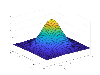
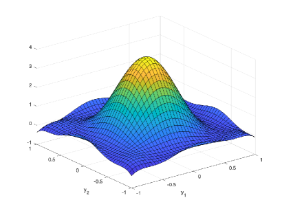
Refer to caption
Refer to caption
Figure 1. Example 1: (a) the exact strength; (b) the reconstructed strength at a single frequency k=2𝑘2k=2.

Example 1: Reconstruct the strength function given by

μ(y1,y2)=4e4(y12+y22),y=(y1,y2)D.formulae-sequence𝜇subscript𝑦1subscript𝑦24superscript𝑒4superscriptsubscript𝑦12superscriptsubscript𝑦22𝑦superscriptsubscript𝑦1subscript𝑦2top𝐷\mu(y_{1},y_{2})=4e^{-4(y_{1}^{2}+y_{2}^{2})},\quad y=(y_{1},y_{2})^{\top}\in D.

The exact strength μ𝜇\mu is plotted in Figure 1(a). For the reconstruction, we choose the iteration number of the outer loop L=6𝐿6L=6 and the regularization parameter γ=107𝛾superscript107\gamma=10^{-7}. Figure 1(b) plots the reconstructed strength by using a single frequency k=2𝑘2k=2. It is clear to see that the bump of the exact strength is well reconstructed by using data with only one frequency. The reason is that the strength function only contains few low frequency Fourier modes and all the high frequency Fourier modes decay exponentially fast.

Example 2: Reconstruct the strength function give by

μ(y1,y2)=μ~(3y1,3y2),𝜇subscript𝑦1subscript𝑦2~𝜇3subscript𝑦13subscript𝑦2\mu(y_{1},y_{2})=\tilde{\mu}(3y_{1},3y_{2}),

where

μ~(y1,y2)=0.3(1y1)2ey12(y2+1)2(0.2y1y13y25)ey12y220.03e(y1+1)2y22.~𝜇subscript𝑦1subscript𝑦20.3superscript1subscript𝑦12superscript𝑒superscriptsubscript𝑦12superscriptsubscript𝑦2120.2subscript𝑦1superscriptsubscript𝑦13superscriptsubscript𝑦25superscript𝑒superscriptsubscript𝑦12superscriptsubscript𝑦220.03superscript𝑒superscriptsubscript𝑦112superscriptsubscript𝑦22\tilde{\mu}(y_{1},y_{2})=0.3(1-y_{1})^{2}e^{-y_{1}^{2}-(y_{2}+1)^{2}}-(0.2y_{1}-y_{1}^{3}-y_{2}^{5})e^{-y_{1}^{2}-y_{2}^{2}}-0.03e^{-(y_{1}+1)^{2}-y_{2}^{2}}.

The exact strength μ𝜇\mu is plotted in Figure 2(a). This example is harder since it contains a few more Fourier modes than Example 1. It is expected that the multi-frequency data is needed to reconstruct the strength. To incorporate the data with multiple frequencies, one more outer loop is added to the Kaczmarz algorithm and this loop is taken with respect to the wavenumber k𝑘k. We choose the iteration number of the intermediate loop L=6𝐿6L=6 and the regularization parameter γ=105𝛾superscript105\gamma=10^{-5}. As a comparison, Figure 2(b) shows the reconstruction at a single frequency k=2𝑘2k=2. Clearly, it is insufficient to reconstruct all the details of the true strength by using only a single low frequency data. Figure 2(c) plots the reconstruction by using multi-frequency data at k=1:3:𝑘13k=1:3. The improvement of the reconstruction is obvious and some details of the true strength are already recovered. Figure 2(d) shows the reconstruction by using multi-frequency data at k=1:5:𝑘15k=1:5. As a few more high frequency data is used, it can be seen that almost all the details of the exact strength are recovered.
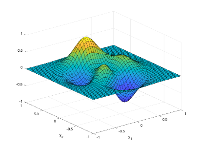
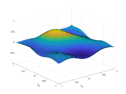
Refer to caption
Refer to caption
Refer to caption
Refer to caption
Figure 2. Example 2: (a) the exact strength; (b) the reconstructed strength at a single frequency k=2𝑘2k=2; (c) the reconstructed strength by using multiple frequencies k=1:3:𝑘13k=1:3; (d) the reconstructed strength by using multiple frequencies k=1:5:𝑘15k=1:5.

6. Conclusion

We have studied the direct and inverse problems for the stochastic biharmonic operator wave equation driven by a microlocally isotropic Gaussian random source whose covariance operator is a classical pseudo-differential operator. Since the source is too rough to exist pointwisely, it can only be interpreted as a distribution. The well-posedness of the direct problem is obtained in the distribution sense for such a rough source. For the inverse problem, we show that a single realization of the magnitude of the wave field averaged over the frequency band is enough to uniquely determine the strength of the random source. Numerical experiments are presented for the white noise model to demonstrate the effectiveness of the proposed method.

Since the inverse source problem is linear, one can get an explicit integral expression of the wave field by using the fundamental solution, which is essential in getting the reconstruction formula. If the medium or potential function is a random field, the framework used in the present work is not applicable anymore since the inverse random potential or medium problem is nonlinear. We refer to [12, 28, 26, 27] for related inverse potential problems for the deterministic equations with the biharmonic operator. It is open for the inverse random potential or medium problem of the biharmonic wave equation. We hope to be able to report the progress on these problems elsewhere in the future.

References

  • [1] M. Abramowitz and I. A. Stegun, editors, Handbook of Mathematical Functions with Formulas, Graphs, and Mathematical Tables, Dover Publications, Inc., New York, 1992.
  • [2] G. Bao, C. Chen, and P. Li, Inverse random source scattering problems in several dimensions, SIAM/ASA J. Uncertainty Quantification, 4 (2016), 1263–1287.
  • [3] G. Bao, C. Chen, and P. Li, Inverse random source scattering for elastic waves, SIAM J. Numer. Anal., 55 (2017), 2616–2643.
  • [4] G. Bao, S.-N. Chow, P. Li, and H. Zhou, An inverse random source problem for the Helmholtz equation, Math. Comp., 83 (2014), 215–233.
  • [5] G. Bao, P. Li, J. Lin, and F. Triki, Inverse scattering problems with multi-frequencies, Inverse Problems, 31 (2015), 093001.
  • [6] P. Caro, T. Helin, and M. Lassas, Inverse scattering for a random potential, Anal. Appl. (Singap.), 17 (2019), 513–567.
  • [7] F. Gazzola, H.-C. Grunau, and G. Sweers, Polyharmonic Boundary Value Problems, Positivity Preserving and Nonlinear Higher Order Elliptic Equations in Bounded Domains, Lecture Notes in Mathematics, Springer-Verlag, Berlin, Heidelberg, 2010.
  • [8] Y. Gong and X. Xu, Inverse random source problem for biharmonic equation in two dimensions, Inverse Probl. Imaging, 13 (2019), 635–652.
  • [9] T. Helin, M. Lassas, and L. Oksanen, Inverse problem for the wave equation with a white noise source, Comm. Math. Phys., 332 (2014), 933–953.
  • [10] H. Holden, B. Øksendal, J. Ubøe, and T. Zhang, Stochastic Partial Differential Equations, A Modeling, White Noise Functional Approach, Second edition, Universitext, Springer, New York, 2010.
  • [11] V. Isakov, Inverse Source Problems, Mathematical Surveys and Monographs, 34, American Mathematical Society, Providence, RI, 1990.
  • [12] K. Krupchyk, M. Lassas, and G. Uhlmann, Determining a first order perturbation of the biharmonic operator by partial boundary measurements, J. Funct. Anal., 262 (2012), 1781–1801.
  • [13] K. Krupchyk, M. Lassas, and G. Uhlmann, Inverse boundary value problems for the perturbed polyharmonic operator, Trans. Amer. Math. Soc., 366 (2014), 95–112.
  • [14] N. S. Landkof, Foundations of Modern Potential Theory, Translated from the Russian by A. P. Doohovskoy, Die Grundlehren der mathematischen Wissenschaften, Band 180, Springer-Verlag, New York-Heidelberg, 1972.
  • [15] M. Lassas, L. Päivärinta, and E. Saksman, Inverse scattering problem for a two dimensional random potential, Comm. Math. Phys., 279 (2008), 669–703.
  • [16] J. Li, T. Helin, and P. Li, Inverse random source problems for time-harmonic acoustic and elastic waves, Comm. Partial Differential Equations, 45 (2020), 1335–1380.
  • [17] J. Li, P. Li, and X. Wang, Inverse elastic scattering for a random potential, arXiv:2007.05790.
  • [18] P. Li and X. Wang, Inverse random source scattering for the Helmholtz equation with attenuation, SIAM J. Appl. Math., 81 (2021), 485–506.
  • [19] P. Li and X. Wang, An inverse random source problem for Maxwell’s equations, Multiscale Model. Simul. 19 (2021), 25–45.
  • [20] P. Li and X. Wang, Regularity of distributional solutions to stochastic acoustic and elastic scattering problems, J. Differential Equations, 285 (2021), 640–662.
  • [21] P. Li, X. Yao, and Y. Zhao, Stability for an inverse source problem of the biharmonic operator, arXiv:2102.04631.
  • [22] A. Lodhia, S. Sheffield, X. Sun, and S. Watson, Fractional Gaussian fields: a survey, Probab. Surv., 13 (2016), 1–56.
  • [23] N. V. Movchan, R. C. McPhedran, A. B. Movchan, and C. G. Poulton, Wave scattering by platonic grating stacks, Proc. R. Soc. A, 465 (2009), 3383–3400.
  • [24] J. Rousseau and L. Robbiano, Spectral inequality and resolvent estimate for the bi-harmonic operator, J. Eur.Math. Soc., 22 (2020), 1003–1094.
  • [25] A. P. S. Selvadurai, Partial Differential Equations in Mechanics 2 The Biharmonic Equation, Poisson’s Equation, Springer-Verlag, Berlin, 2000.
  • [26] T. Tyni and M. Harju, Inverse backscattering problem for perturbations of biharmonic operator, Inverse Problems, 33 (2017), 105002.
  • [27] T. Tyni and V. Serov, Scattering problems for perturbations of the multidimensional biharmonic operator, Inverse Probl. Imaging, 12 (2018), 205–227.
  • [28] Y. Yang, Determining the first order perturbation of a bi-harmonic operator on bounded and unbounded domains from partial data, J. Differential Equations, 257 (2014), 3607–3639.