Multi-objective Asynchronous Successive Halving

Abstract

Hyperparameter optimization (HPO) is increasingly used to automatically tune the predictive performance (e.g., accuracy) of machine learning models. However, in a plethora of real-world applications, accuracy is only one of the multiple – often conflicting – performance criteria, necessitating the adoption of a multi-objective (MO) perspective. While the literature on MO optimization is rich, few prior studies have focused on HPO. In this paper, we propose algorithms that extend asynchronous successive halving (ASHA) to the MO setting. Considering multiple evaluation metrics, we assess the performance of these methods on three real world tasks: (i) Neural architecture search, (ii) algorithmic fairness and (iii) language model optimization. Our empirical analysis shows that MO ASHA enables to perform MO HPO at scale. Further, we observe that that taking the entire Pareto front into account for candidate selection consistently outperforms multi-fidelity HPO based on MO scalarization in terms of wall-clock time. Our algorithms (to be open-sourced) establish new baselines for future research in the area.

1 Introduction

With the increasing complexity of deep neural networks (DNNs), such as convolutional neural networks (CNNs) Lecun1999:Object and Transformers Vaswani2017:Attention , the task of tuning their hyperparameters has become critically important, but also time-consuming and costly. To automate this process, hyperparameter optimization (HPO) is routinely used to maximize predictive performance. However, in many real-world applications, predictive performance is not the only relevant performance objective. Instead, users are interested in simultaneously optimizing several objectives such as fairness, interpretability or latency. For instance, prior work has shown that improving fairness can have an adverse impact on model accuracy corbett2017algorithmic and that optimizing fairness w.r.t. one metric can deteriorate others kleinberg2016inherent . Similarly, while increasing the size of a LSTM-based language model can lead to improvements in perplexity, it can also significantly increase the prediction cost Strubell2019:Energy .

Despite the pervasiveness of multi-objective (MO) problems in the context of HPO, the area of multi-objective hyperparameter optimization (MO-HPO) has received little attention from the research community so far. While a few studies exist, most notably, based on multi-objective Bayesian optimization (MBO), these are limited to a narrow range of tasks Lobato2016 (i.e. fast and accurate neural networks for MNIST Lecun1998:MNIST ) and the empirical analysis is limited; evaluations are often performed on synthetic functions and/or focuses on a small number of objectives, usually no more than three.

In this paper, we extend asynchronous successive halving (ASHA) Li2018:Massively , which is a scheduler for distributed multi-fidelity HPO, to the MO setting. As is standard when optimizing several objectives simultaneously, we cast the problem as that of approximating the Pareto front. The Pareto front is the set of all non-dominated solutions to the MO problem; these are the solutions for which none of the objectives can be improved without degrading another one. Recovering the Pareto is convenient in practice as it enables users to navigate the optimal trade-off between the multiple objectives.

Our goal is to efficiently recover well-rounded fronts in real-world scenarios. The gradient-free MO optimization algorithms we introduce leverage an asynchronous successive halving scheduler (ASHA) Li2018:Massively and rely on MO optimization strategies based on scalarizing the objective vector (e.g., scalarization technique of Knowles2006:Parego ; Golovin2020 ), as well as approaches that take the geometry of the whole Pareto front into account (e.g., the non-dominated sorting technique of Deb2002:Fast ). The resulting MO-HPO algorithms benefit from early stopping and parallelization to deliver significant performance gains over existing MBO techniques.

We evaluate the performance of these algorithms using several performance metrics such as dominated hypervolume Zitzler1998:Multiobjective and quality of the minimax solution. We also investigate how different algorithms navigate the solution space over time and the speed at which they recover the Pareto front. We perform an empirical comparison across a diverse range of MO tasks ranging from fairness-aware learning over neural architecture search to language modeling. Results indicate that techniques that take the geometry of the current Pareto front approximation into account perform consistently better than the scalarization-based techniques across different tasks. In fact, in some cases, the scalarization-based techniques are not significantly better than a random search over the hyperparameter space.

To summarize, our main contributions are:

1. We obtain multi-fidelity HPO algorithms by extending ASHA to the MO setting, considering scalarization-based selection techniques, as well as techniques informed by the geometry of the Pareto front.

2. We evaluate these multi-fidelity MO-HPO algorithms on a range of real-world tasks and evaluation metrics, showing that they can be used effectively to navigate trade-offs between various objectives.

3. We show that exploration schemes informed by the geometry of the Pareto front outperform the scalarization based techniques on HPO problems.

2 Related Work

BO allows to build cheap to evaluate surrogate models that can be used to trade-off exploration and exploitation. Multi-objective Bayesian optimization (MBO) techniques have been developed and can be categorized into three classes. First, scalarization-based MBO methods map the vector of all objectives to a single scalar value Knowles2006:Parego ; Zhang2009:Expensive ; Nakayama2009:Sequential ; Paria2019:Flexible ; Zhang2020:Random ; Golovin2020 and then use conventional single-objective (SO) BO techniques. While these methods are comparatively easy to implement and scale gracefully with the number of objectives, they are not guaranteed to convergence to the full Pareto front with the notable exception of Golovin2020 . A second class of MBO techniques optimize a performance measure of Pareto front approximations, namely the dominated hypervolume Zitzler1998:Multiobjective . Both the expected hypervolume improvement (EHI) Emmerich2011:Hypervolume and probability of hyper-improvement (PHI) Keane2006:Statistical extend their single-objective BO counterparts, the expected improvement Mockus1978:Application ; Jones1998:Efficient and the probability of improvement Kushner1964:New , respectively. Other methods include step-wise uncertainty reduction (SUR) Picheny2015:Multiobjective , smsEGO Ponweiser2008:Multiobjective ; Wagner2010:Expected and expected maximin improvement (EMMI) Svenson2010:Multiobjective . Third, information-theoretic MBO approaches have been proposed. They aim to reduce uncertainty about the location of the Pareto front. Methods in this class tend to be more sample efficient and scale better with the number of objectives. PAL Zuluaga2013:Active iteratively reduces the size of a discrete uncertainty set. PESMO Hernandez2016:Predictive adapts the predictive entropy search (PES) Hernandez2014:Predictive criterion. Pareto front entropy search (PFES) Suzuki2019:Multi is suitable when dealing with decoupled objectives. MESMO Belakaria2019:Max builds on the max-value entropy-search criterion Wang2017:Max and enjoys an asymptotic regret bound. Building on MESMO, two recent works have proposed MF-OSEMO Belakaria2020:Multi and iMOCA Belakaria2020:Information , two multi-fidelity based information-theoretic MBO techniques which internally use continuous fidelity Gaussian processes.

MO evolutionary algorithms (EA) identify promising solution candidates that are close to the Pareto front and mutate them to conduct exploration Elsken2019 . At the heart of many EA methods lies non-dominated-sorting srinivas1994 which ranks candidates in a two stage process. First, candidates are grouped into multiple distinct Pareto fronts by iteratively computing a front and reducing the candidate set until all points are assigned. Second, candidates inside the individual fronts are ranked using crowding distance Deb2002:Fast to encourage uniform exploration. We refer to Emmerich2018 for a survey on EA approaches.

Rather than evaluating poor models for the maximum resource budget, typically epochs, multi-fidelity HPO iteratively allocates resources to hyperparameter configurations that perform sufficiently well at certain checkpoints (or rungs). Hyperband Li2017Hyperband is an extension of Successive Halving Jamieson2016:Non which samples random candidates, compares their performance after their intermediate budget allocation is exhausted, and only let the most promising candidates run for larger computational budgets. Waiting for all configurations to finish to make a stopping decision is wasteful as it causes idle workers. ASHA Li2018:Massively is an asynchronous extension of Hyperband, yielding a large improvement in wall clock time. Recently, Schmucker2020:Multi applied simple scalarization (i.e., linear mixture of objectives) to Hyperband and Salinas2021:Multi investigated the combination of EA and Hyperband when considering tuning hyperparameters and hardware jointly. Finally a parallel work investigates the performance of different MF approaches when optimizing only two objectives for computer-vision tasks guerrero2021 . In our work, we adapted the non-dominating sorting idea from EA with an ASHA-style early-stopping mechanism, investigating the performance of the proposed methods in several different scenarios, from NAS to Algorithmic Fairness optimizing over many different objectives.

3 Background: Multi-Objective Optimization (MO)

The MO problem

In many real world settings there is not just one, but multiple potentially conflicting objectives of interest. For example when working with hardware constraint systems one desires predictive models that are accurate and have low resource consumption. Assume one needs to decide between two solutions $\bm{x}_{1},\bm{x}_{2}$. Each individual objective induces a distinct ordinal relationship between the candidates, but while $\bm{x}_{1}$ might dominate $\bm{x}_{2}$ in one objective it might be worse in another. Because there is rarely a single best solution, the MO problem is to identify the Pareto front – the set of all non-dominated solutions – to help users to make an informed trade-off.

More formally, let $f:\mathcal{X}\rightarrow\mathbb{R}^{n}$ be a function over domain $\mathcal{X}$ that we aim to minimize. Given two points $\bm{x}_{1},\bm{x}_{2}\in\mathcal{X}$, we write $\bm{x}_{1}\succeq\bm{x}_{2}$ if $\bm{x}_{2}$ is weakly-dominated by $\bm{x}_{1}$, that is, iff $f(\bm{x}_{1})_{i}\leq f(\bm{x}_{2})_{i},\forall i\in[n]$. We write $\bm{x}_{1}\succ\bm{x}_{2}$ if $\bm{x}_{2}$ is dominated by $\bm{x}_{1}$, that is, iff $\bm{x}_{1}\succeq\bm{x}_{2}$ and $\exists i\in[n]$ s.t. $f(\bm{x}_{1})_{i}<f(\bm{x}_{2})_{i}$. The Pareto front of $f$ is defined by $\mathcal{P}_{f}=\{\bm{x}\in\mathcal{X}|\not\exists\bm{x}^{\prime}\in\mathcal{X}:\bm{x}^{\prime}\succ\bm{x}\}$, that is, the set of all non-dominated points. As $\mathcal{P}_{f}$ is often an infinite object, MO algorithms aim to recover an approximation set $A\subset\mathcal{X}$ of non-dominated objective vectors. A popular measure of approximation quality is the dominated hypervolume Zitzler1998:Multiobjective . Given an approximation set $A$ and a reference point $\bm{r}$ the hypervolume indicator $\mathcal{H}$ is given by:

$$\mathcal{H}(A)=\text{Vol}\left(\{\bm{x}\in\mathbb{R}^{n}|\exists\bm{z}\in A:\bm{z}\succeq\bm{x}\wedge\bm{x}\succeq\bm{r}\}\right).$$ (1)

Hypervolume related quantities are usually computed by partitioning the space into hyper-cubes which are then summed. This operation scales exponentially with the number objective functions and can cause a bottleneck for related MO optimization approaches.

Scalarization for MO

Scalarization techniques reduce the MO to an SO problem by optimizing a linear combination of the multiple competing objectives. For some $\bm{w}\in\mathbb{R}^{n}$, solving the MO minimization problem consists in solving the following optimization problem:

$$\min_{\bm{x}\in\mathcal{X}}V(f(\bm{x},r_{t}),\bm{w}),$$ (2)

where $V:\mathbf{R}^{n}\times\mathbf{R}^{n}\rightarrow\mathbf{R}$ is a scalarization function of choice. Some concrete choices of $V$ are the inner product between objective and weight vector (also known an Random Weights) and the scalarization functions employed by ParEGO Knowles2006:Parego and Golovin Golovin2020 :

$$\begin{split}V_{\text{RW}}(\bm{y},\bm{w})=\bm{y}^{\top}\bm{w},\quad V_{\text{ParEGO}}(\bm{y},\bm{w})=\max_{j\in\{1,\dots,n\}}(w_{j}y_{j})+\rho(\bm{y}^{\top}\bm{w})\\ V_{\text{Golovin}}(\bm{y},\bm{w})=\min_{j\in\{1,\dots,n\}}(\max(0,y_{j}/w_{j}))^{n}.\quad\quad\quad\quad\quad\end{split}$$ (3)

4 Distributed Asynchronous Multi-objective Hyperparameter Optimization

Our work builds on Schmucker2020:Multi . The authors evaluated various MBO techniques on MO-HPO tasks and artificial functions (an excerpt of their study is provided in Appendix C). They reported, perhaps surprisingly, that in many cases random search could yield a sample complexity comparable to BO in the MO setting, while being easy to parallelize. Motivated by these observations, they proposed a Hyperband-style algorithm that uses random scalarization for hyperparameter candidate selection. Given a computational budget, single objective Hyperband Li2017Hyperband starts by providing a small initial resource allocation $r_{0}$ to each randomly sampled model configuration. If a configuration does not seem promising after its allocation is exhausted (e.g., in terms of validation error), Hyperband uses an early-stopping rule to terminate unpromising candidates and reallocates (larger) additional resource $r_{t}$ to the most promising ones. This process is repeated until the total budget is exhausted. Hyperband extends the Successive Halving algorithm Jamieson2016:Non by introducing an additional parameter $\eta$ which is used to trade-of the number candidate hyperparameters with a per candidate budget.

To adapt Hyperband to the MO domain, Schmucker2020:Multi use scalarization to reduce each configuration’s evaluation vector to a single real valued scalar which allows for an easy candidate ranking. For this each individual configuration $\bm{x}\in\mathcal{X}$ is equipped with a distinct set of $m$ vectors $W=\{\bm{w}_{1},\dots,\bm{w}_{m}\}$ sampled uniformly from $\Delta_{n}$ (i.e., the set of all vectors in the positive orthant with entries summing up to one). The performance of configuration $\bm{x}$ after partial training is then measured by

$$e_{V}(\bm{x},W,r_{t})=\min_{\bm{w}\in W}V(f(\bm{x},r_{t}),\bm{w}).$$ (4)

While the use of scalarization techniques is a convenient response to the candidate selection problem, as it allows the application of single objective BO, it comes with multiple shortcomings. It is known that scalarization techniques can only capture restricted Pareto shapes Golovin2020 . Moreover, each individual weight vector only encourages exploration in a single direction and, if the set of weight vectors $W$ is not chosen carefully, it can fail to recover the full Pareto front altogether. The use of linear scalarization schemes also tends to focus heavily on the objective value of smallest magnitude which can cause failure for non-convex Pareto fronts. Finally, scalarization techniques are heavily affected by rescaling of objective values.

1 function non_dom_sorting($P$)

2       $i=1$

3       while $P\neq\emptyset$ do

4             $F_{i}\leftarrow\{\bm{\theta}\in P:\bm{\theta}\,\,\text{non-dominated}\}$

5             $(P,\,i)\leftarrow(P\setminus F_{i},\,i+1)$

6            

7      return $F_{1},\dots,F_{m}$

8      

 

9 function selector_eps_net($P$, $n$)

10       $F_{1},\dots,F_{m}\leftarrow\texttt{non\_dom\_sorting}(P)$

11       $\mathcal{C}\leftarrow[F_{1}\text{.pop}()]$

12       for $F=F_{1},\dots,F_{m}$ do

13             while $F\neq\emptyset$ do

14                   $\bm{\theta}\leftarrow\min_{\bm{\theta}\in F}\max_{\bm{\theta}^{\prime}\in\mathcal{C}}\|\bm{y}_{\bm{\theta}}-\bm{y}_{\bm{\theta}^{\prime}}\|_{2}$

15                   $\mathcal{C}\text{.append}(\bm{\theta})$

16                   $F\leftarrow F\setminus\{\bm{\theta}\}$

17                  

18      return $\mathcal{C}_{1},\dots,\mathcal{C}_{n}$

19      

 

20 function selector_nsga_ii($P$, $n$)

21       $F_{1},\dots,F_{m}\leftarrow\texttt{non\_dom\_sorting}(P)$

22       $\mathcal{C}\leftarrow[\,]$

23       for $F=F_{1},\dots,F_{m}$ do

24             $\mathcal{C}\leftarrow\mathcal{C}+\texttt{crowding\_dist\_sorting}(F)$

25            

26      return $\mathcal{C}_{1},\dots,\mathcal{C}_{n}$

27      

Algorithm 1 Multi-objective selector

Data: $R$, $r_{0}$, $s$, $\eta$ (default $\eta=3$)

1 function mo_asha()

2       repeat

3             for each free worker do

4                   $(\bm{\theta},k)\leftarrow\texttt{get\_job}()$

5                   run_evaluation($\bm{\theta}$, $r_{0}\eta^{s+k}$)

6                  

7            for completed job $(\bm{\theta},k)$ with objective vector $\bm{y}_{\bm{\theta}}$ do

8                   update $\bm{\theta}$ in rung $k$ with $\bm{y}_{\bm{\theta}}$

9                  

10      until budget exhausted

 

11 function get_job()

12       for $k=\lfloor\log_{\eta}(R/r_{0})\rfloor-s-1,\dots,1,0$ do

13             $\text{candidates}\leftarrow\texttt{mo\_selector}(\text{rung}\,k,\left|\text{rung}\,k\right|/\eta)$

14             $\text{promotable}\leftarrow\{\bm{\theta}\in\text{candidates}:\bm{\theta}\,\,\text{not promoted}\}$

15             if $\,|\text{promotable}|>0$ then

16                   return (promotable[0], $k+1$)

17                  

18      draw random configuration $\bm{\theta}$

19       return $(\bm{\theta},0)$

20      

Algorithm 2 Multi-objective ASHA

To mitigate these issues we propose to move away from scalarization.

Instead, we make use of non-dominating sorting for budget allocation. In particular we adapt the NSGA-II Deb2002:Fast selection mechanism and the $\epsilon$-net Salinas2021:Multi (EpsNet) exploration strategy which ranks candidates in the same Pareto front by iteratively selecting the candidate with the largest euclidean distance from the set previously selected configurations. The pseudo-code for non-dominating sorting is presented in Algorithm 1, as well as the structure of EpsNet and NSGA-II. They both use a non-dominating sorting sub-routine, and they differ by their internal inner selection loop (please refer to the original NSGA-II paper Deb2002:Fast for a complete definition of crowding_dist_sorting). In contrast to scalarization based techniques which assign a single value to each candidate independently of other configurations, EpsNet and NSGA-II use information about the global geometry of the Pareto front approximation. They use non-dominating sorting to categorize evaluated candidates into multiple fronts and rank candidates in the individual fronts in a way that encourages a uniform coverage of the true Pareto front. By making decisions informed by the global geometry of the current Pareto front approximation these selections strategies encourage a more uniform exploration of the different objectives and are less impacted by objective values of different magnitudes.

We further replace the distributed synchronous scheduler used in Hyperband by the distributed asynchronous scheduler used in ASHA to improve wall-clock time. In each rung (i.e., a round of resources consumed), Hyperband waits until all configurations have exhausted their resource allocation. Especially when optimizing large neural networks where some configurations take much longer to evaluate than others this can be expensive because it causes idle workers. ASHA avoids this issue by assigning workers new configurations as soon as they terminate their current evaluation. It does so by operating on multiple rungs in parallel and by making its allocation decision based on partial information. This procedure has been shown to yield large wall-clock time improvements in the single objective setting. An overview of our proposed method is provided by Algorithm 2. It defines a family of MO-ASHA algorithms that can be equipped with candidate selection strategies. As concrete choices of selection strategies we experimentally evaluate the three scalarization schemes from Equation 3 as well as the non-dominated sorting strategies NSGA-II and EpsNet.

5 Multi-objective Optimization Tasks

We consider three challenging MO hyperparameter optimization problems as detailed next.

Task 1: Neural Architecture Search (NAS)

The goal of neural architecture search (NAS) is to automatically find network architectures where the search space may include number of convolutional layers, size of the convolutions or type of pooling. While initial works aims only at finding architectures with high prediction accuracy zoph2017neural , deploying such models (e.g., on the edge) also requires to consider other objectives such as cost or latency. We refer to Benmeziane2021 for a survey on hardware-aware NAS. In particular, scalarization schemes have been considered in Computer Vision Tan2018 ; Wu2019 , where the objectives were mapped to a single real value via a fixed set of weights trying to achieve a good trade-off. Having to fix the weights a priori is impractical and restrictive as each specific scalarization can only capture restricted Pareto shapes Golovin2020 . Other approaches such as Elsken2019 propose to tailor EA to NAS by modeling the nature of the multiple competing objectives explicitly. Considering these recent trends, we conducted experiments on the NAS-201 benchmark  Dong2020:Nasbench201 which contains tabular evaluations of accuracy and latency for 15625 architectures on 3 datasets.

Task 2: Algorithmic Fairness

Algorithmic fairness aims to train accurate models subject to fairness criteria. Prior work has proposed several fairness criteria, whose suitability depends on the application domain, and it has been shown that criteria,commonly referred to acceptance-based and error-based, can be in conflict with each other friedler2016possibility ; fairness2018verma ; kleinberg2018inherent .

Let $Y$ be the true label, $\hat{Y}$ the predicted label, and $S$ a binary sensitive attribute (i.e., the population is formed by two subgroups). We consider the following criteria:

• Statistical Parity (SP) requires equal Positive Rates (PR) across subgroups: $P(\hat{Y}=1|S=0)=P(\hat{Y}=1|S=1)$,

• Equal Opportunity (EO) requires equal True Positive Rates (TPR) across subgroups: $P(\hat{Y}=1|Y=1,S=0)=P(\hat{Y}=1|Y=1,S=1)$;

• Equalized Odds (EOdd) requires equality of False Positive Rates (FPR) in addition to EO.

The extension to more than two sensitive features values and more than two classes is straightforward.

In general, algorithmic fairness methods can be divided into three families: (i) post-processing to modify a pre-trained model to increase the fairness of its outcomes feldman2015certifying ; hardt2016equality ; pleiss2017fairness ; (ii) in-processing to enforce fairness constraints during training agarwal2018reductions ; donini2018empirical ; zafar2017fairness ; zafar2019fairness ; and (iii) pre-processing to modify the data representation and then apply standard machine learning algorithms calmon2017optimized ; zemel2013learning . Most of approaches provide solutions for only a single fairness metric. For example, feldman2015certifying is limited to demographic parity definition of fairness. In contrast to in-processing methods, which are often dependent on the model class (e.g., zafar2017fairness ; Zhang2018 ; donini2018empirical ) and hence have limited extensibility, using MO-HPO allows us to consider any fairness constraint and while being agnostic to the specific model as it operates only on its hyperparameters.

Task 3: Training Language Models

Language modeling assign a probability value to a given input text sequence $\mathbf{t}=(t_{1},t_{2},\ldots,t_{T})$ by modeling individual token probabilities as $p(\mathbf{t})=\prod_{i=1}^{T}p(t_{i}|t_{1},t_{2},\ldots,t_{i-1})$. The most popular evaluation metric for language models (LM) is perplexity over a held-out set. A high perplexity indicates that the LM is “surprised” to see the input sequences. As a result, a low perplexity is a desirable property. However, perplexity is shown to not always correlate with other desirable metrics such as word error rate Chen1998:Evaluation . Word error rate measures the accuracy of the LM in predicting the next word by comparing the word that is predicted to be most likely by the LM with the ground truth next word in the sequence. Moreover, while larger LMs can lead to lower perplexity, it may also result in higher prediction time due to increased network size. In this work, we consider Transformer-based LMs that not only minimize perplexity, but also lead to low prediction time and low word error rate.

6 Experiments

We evaluate our approach on the three different HPO tasks discussed in Section 5: (i) Neural architecture search using NAS-201 benchmark Dong2020:Nasbench201 , (ii) algorithmic fairness training MLP models on Adult dataset Kohavi1996:Scaling and (iii) Transformer language models optimization on Wikitext2 Merity2016:Pointer corpus. Hyperparameter spaces are provided by Tables 2, 3 and 4 in Appendix A. We compare MO-ASHA implementations employing 3 different scalarization techniques (RW, ParEGO, Golovin), 2 globally informed selection strategies (NSGA-II, EpsNet) and random search (RS) baseline. Following Schmucker2020:Multi each scalarization method is equipped with 100 random vectors. As ASHA hyperparameters we chose reduction factor $\eta=3$, minimum resource budget $r_{0}=1$ and maximum budget $R=200$ for NAS-201 and Adult and $R=81$ for Wikitext2. For our evaluations, we normalize all objectives values with quantiles using the empirical CDF which scales objective ranges to the $[0,1]$ interval making our comparisons robust to monotonic transformations of the objectives Binois2020 . This allows us to compute the dominated hypervolume with respect to worst case reference point $\vec{1}\in\mathbb{R}^{n}$. For Adult and Wikitext2 a reference Pareto front approximation $\mathcal{A}$ is formed by accumulating the evaluations from all runs and epochs. The tabular nature NAS-201 allows us to determine the exact Pareto front.

NAS-201 benchmark dataset

Figure 1: Left: Difference in dominated hypervolume of the Pareto front approximations for the different methods with respect to the real Pareto front approximation over time for ImageNet16-120 dataset. The objectives of interest are two: error (ERR) and prediction time (TIME). Right: Pareto fronts found by the different methods for the same dataset, compared to the ground truth Pareto front (i.e., the best Pareto front that can be obtained from NAS-201 network architectures).

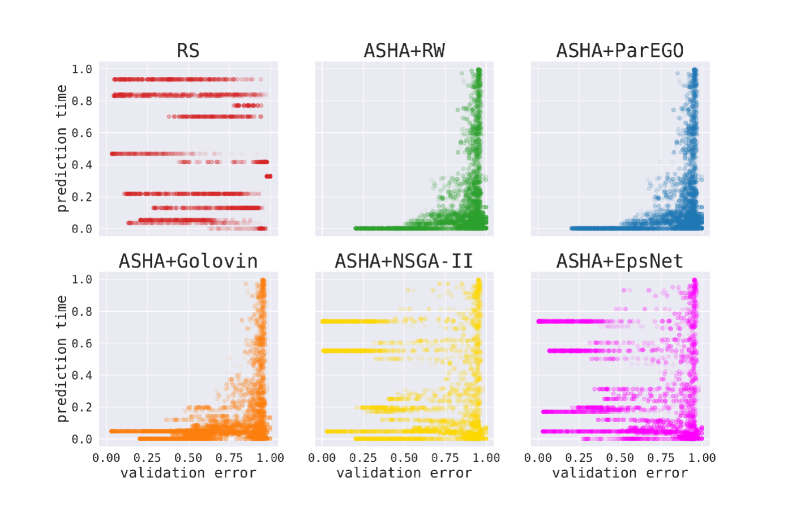
Figure 2: Objective values visualizing how different methods explore the NAS-201 ImageNet16-120 architecture space over time. Each model evaluation is represented by a single dot. Darker color indicates that the model has been evaluated later in time during the search.

In the first experiment we search for fast and accurate Res-Net architectures using the tabular NAS-201 benchmark dataset. NAS-201 describes a 6-dimensional search space and provides evaluations of 15625 different neural network architectures on 3 datasets. We perform 10 runs using 4 parallel workers on AWS ml.c4.xlarge instances. We set a maximum run time of 3 hours for Cifar-10, 5 hours for Cifar-100 and 8 hours for ImageNet16-120 datasets. We optimize over two objectives: the validation error (ERR) and the prediction or inference time (TIME).

The left side of Figure 1 visualizes the difference in dominated hypervolume of the approximations to the real ImageNet16-120 Pareto front over time. The plot shows the performance of the different methods, highlighting that the group of methods relying on scalarization techniques (RW, ParEGO, Golovin) obtains worse performance than the methods using geometric information (NSGA-II, EpsNet). Especially, EpsNet obtains the best performance at the end of the time budget. In this task, RS performs sufficiently well, outperforming RW and ParEGO, and being very competitive in the first phases of the exploration, due to the full training it performs for each choice of hyperparameters.

The right side of Figure 1 shows the Pareto fronts recovered by the different methods, as well as the ground truth front (i.e., the Pareto front of all possible NAS-201 networks). It is interesting to note how scalarization techniques tend to penalize one objective heavier than the other, focusing on models with very low prediction time, and avoiding the area of the search space with slower more accurate models. This shows the advantage of globally informed algorithms being able to explore the search space more uniformly. In fact, globally informed techniques are more robust towards objectives of different magnitude. Experimental results for Cifar-10 and Cifar-100 datasets are provided in Appendix B. Cifar-100 confirms the insights we presented for ImageNet16-120. Cifar-10 is a rather simple problem and all MO-ASHA variants perform roughly the same.

Finally, another important aspect to analyse is how the different algorithms explore the search space over time. Similar dominated hypervolume can be achieved with different exploration strategies. We visualize the models evaluated by the different methods (considering each epoch as an evaluation) over time in Figure 2 to see which parts of the search space they focus on. Each dot represents an evaluation and darker colors indicates evaluation at a later point in time. We can observe that RW, ParEGO and Golovin tend to focus heavily on finding models with low prediction times and fail to explore slower models that yield the best accuracy. Random search does not show this bias, but suffers from inefficient resource allocation. NSGA-II and EpsNet have a more balanced exploration scheme that on one side explores faster models with good accuracy, but also considers slower candidates which leads to the discovery of very accurate models.

Fair model for Adult dataset

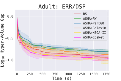
Figure 3: Left: Difference in dominated hypervolume of the Pareto front approximations for the different methods with respect to the combined front approximation over time on Adult with two objectives: ERR and DSP. Right: Pareto fronts found by the different methods on the same dataset.

Table 1: Average validation error (and standard deviation) over 10 repetitions for the best fair models for different methods. We use the fairness constraint: DSP $\leq 0.1$.

Fairness Method	Validation error	MO Method	Validation error
FERM	0.164 $\pm$ 0.010	RS	0.166 $\pm$ 0.005
Zafar	0.187 $\pm$ 0.001	ASHA+RW	0.166 $\pm$ 0.001
Adversarial	0.237 $\pm$ 0.001	ASHA+ParEGO	0.167 $\pm$ 0.003
FERM pre-processed	0.228 $\pm$ 0.013	ASHA+Golovin	0.164 $\pm$ 0.002
SMOTE	0.178 $\pm$ 0.005	ASHA+NSGA-II	0.165 $\pm$ 0.003
CBO MLP	0.167 $\pm$ 0.017	ASHA+EpsNet	0.166 $\pm$ 0.004

For the second set of experiments we selected the Adult Kohavi1996:Scaling dataset and search for MLP models that are both accurate and fair with respect to a sensitive attribute. The Adult dataset is based on census data, and contains binary gender as sensitive attribute. The binary classification task is to predict if the annual income of an individual exceeds 50K USD. This dataset is commonly used to compare the performance of different algorithmic fairness techniques. The search space of considered MLP models is 10 dimensional. Because the dataset is rather small and training a model until convergence is fast we reduced the maximum run time to 30 minutes. We perform 10 runs using 4 parallel workers on AWS ml.c4.xlarge instances and use a 70%/30% random split to form training and validation set.

We train MLP models, optimizing for low validation error (ERR) and different fairness objectives: Statistical Parity (SP), Equal Opportunity (EO) and Equalized Odds. Specifically, we use the violation of the fairness constraint as a measure of unfairness (i.e., objective). In the case of EO, we introduce difference in equal opportunity (DEO), that is the absolute value of the difference of the TPRs between the two sub-groups. And, analogously, we define difference in statistical parity (DSP) and difference in false positive rates (DFP).

The left side of Figure 3 visualizes the difference in dominated hypervolume of the individual front approximations to combined approximation $\mathcal{A}$ over time. The experiments confirm the observations made in the NAS setting. NSGA-II and EpsNet outperform the other methods, with Golovin performing slightly better than RW and ParEGO performing worst. Interestingly, in this task, RS proves to be a competitive baseline at the very beginning (due to complete model training for each parameter choice) and at the end of the 30 minute runs. Aligning with these observations, Appendix B shows results for 3- and 4-objective settings combining various fairness criteria. The right side of Figure 3 visualizes the Pareto front approximations recovered by the different methods. Unlike in the NAS-201 experiments we do not have access to the ground truth Pareto front. Interestingly, this Pareto front is concave which explains the poor performance of linear scalarization methods as they can only recover convex fronts.

It is important to note how using a MO approach allows us to be agnostic towards the underlying machine learning algorithm and combination of objectives (here fairness constraints). This is crucial considering that many the state-of-the-art algorithmic fairness methods can only accommodate specific models or specific fairness definitions. In order to compare the models obtained using the MO approaches to state-of-the-art algorithmic fairness methods we followed the same experimental setting proposed in perrone2020fair and Schmucker2020:Multi . We select a single measure of fairness, i.e. DSP, and find the model with highest accuracy such that the DSP value is less or equal $0.1$. This is a common scenario in algorithmic fairness, where $0.1$ DSP is often considered acceptable.

In Table 1, we report the results of this experiment, comparing MO algorithms versus the following algorithmic fairness methods: Zafar zafar2017fairness , Adversarial debiasing Zhang2018 , Fair Empirical Risk Minimization (FERM and FERM pre-processed) donini2018empirical , constrained BO approach (CBO) for fair models perrone2020fair , and SMOTE chawla2002smote . These results, show that the MO approach is very competitive compared to model- and constraint-specific methods (FERM, Zafar, Adversarial), and also without knowing a priori the threshold of our fairness constraint (as instead needed for CBO).

Language Models for Wikitext2 dataset

Figure 4: Left: Difference in dominated hypervolume of the Pareto front approximations for the different methods with respect to the combined front approximation over time on Wikitext2 with two objectives: PPL and ERR. Right: Pareto fronts found by the different methods on the same dataset.

In the last set of experiments we optimize Transformer based language models on the Wikitext2 corpus for perplexity (PPL), word error rate (ERR) and inference time (TIME). The search space described in Appendix A captures 6 dimensions. We perform 5 runs using a single worker on AWS ml.g4dn.xlarge instances and set the maximum run time to 12h. This experiment is computationally demanding which forced us to perform fewer runs. In total we used 720 GPU hours / 1 GPU month.

The left side of Figure 4 visualizes the difference in dominated hypervolume of the Pareto front approximations to combined Pareto front approximation $\mathcal{A}$. All methods except random search perform roughly the same during the first 3h of the experiment. ParEGO and Golovin show good performance towards the 7h mark. Towards the end of the time budget, EpsNet obtains the best Pareto front approximations. The right side of Figure 4 shows the Pareto fronts recovered by the different methods. Unlike in the two prior experiments perplexity and word error rate are not very conflicting with each other and the main problem is to decide which models to allocate the computational budget too. Taking a look at the performance of random search it is easy to see that naive random sampling does not lead to satisfactory performance. Figure 10 in Appendix B visualizes how the different exploration strategies explore the search space over time. We observe correlation between perplexity and word error rate objectives. Compared to the experiments on the other datasets we are only able to evaluate a rather small number of configurations. Random search spends a lot of computational resources on configurations that turn out to be unsuitable. Overall, the figure underlines the point that the main challenge in this task is efficient resource allocation. Given a larger computational budget it would be interesting to see how the different approaches compare to each other at a point of saturation (i.e. how long does it take each method until it does not discover further useful candidates).

7 Conclusion

In this paper we presented multiple extensions of ASHA to MO in the context of HPO. We evaluated the performance of several methods across three distinct tasks: neural architectural search, algorithmic fairness and language modeling, where the goal of optimizing multiple objectives rises naturally. Our experiments showed that MO ASHA enables MO HPO at scale. Our empirical analysis showed the best performance when MO ASHA is used in synergy with EpsNet selection mechanism to utilize the global geometry of the Pareto front approximation. Our proposal outperforms multi-fidelity HPO based on multi-objective scalarization with respect to the wall-clock time performances by a large margin. All the implemented algorithms will be open-sourced in AutoGluon agtabular .

Appendix A Experimental Setup

Adding to Section 6, we provide additional details about the experimental setup. Descriptions of the hyperparameter spaces used for the NAS-201, Adult, and Wikitext2 experiments are provided by Tables 2, 3 and 4 respectively. For parameters that capture values ranging across multiple orders of magnitude we apply a logarithmic scaling. The NAS-201 and Adult experiments were all performed using AWS ml.c4.xlarge instances providing 4 cores of an Intel Xeon E5-2666 v3 CPU as well as 7.5GB of RAM. For the Wikitext2 experiments we used AWS ml.g4dn.xlarge instances providing 4 cores of a second generation Intel Xeon Cascade Lake CPU, 16GB of RAM as well as one NVIDIA T4 Tensor Core GPU. For the Adult experiment we used Scikit-learn [43] (version 0.24) and for the Wikitext2 experiment we used PyTorch [42] (version 1.8.1).

Table 2: NAS-201, ResNet search space

Parameter	Type	Domain
$x_{0}$	categorical	{skip_connect, conv_1x1, conv_3x3, pool_3x3, none }
$x_{1}$	categorical	{skip_connect, conv_1x1, conv_3x3, pool_3x3, none }
$x_{2}$	categorical	{skip_connect, conv_1x1, conv_3x3, pool_3x3, none }
$x_{3}$	categorical	{skip_connect, conv_1x1, conv_3x3, pool_3x3, none }
$x_{4}$	categorical	{skip_connect, conv_1x1, conv_3x3, pool_3x3, none }
$x_{5}$	categorical	{skip_connect, conv_1x1, conv_3x3, pool_3x3, none }

Table 3: Adult, Sklearn MLP search space

Parameter	Type	Domain	Scaling
n_layers	integer	$\{1,2,3,4\}$	linear
layer_1	integer	$\{2,\dots,32\}$	linear
layer_2	integer	$\{2,\dots,32\}$	linear
layer_3	integer	$\{2,\dots,32\}$	linear
layer_4	integer	$\{2,\dots,32\}$	linear
alpha	real	$[10^{-6},\dots,10^{-1}]$	logarithmic
learning_rate_init	real	$[10^{-6},\dots,10^{-2}]$	logarithmic
beta_1	real	$[0.001,0.99]$	logarithmic
beta_2	real	$[0.001,0.99]$	logarithmic
tol	real	$[10^{-5},10^{-2}]$	logarithmic

Table 4: Wikitext2, Transformer search space

Parameter	Type	Domain	Scaling
lr	real	$[1,50]$	logarithmic
dropout	real	$[0,0.99]$	linear
batch_size	integer	$\{8,\dots,256\}$	linear
clip	real	$[0.1,2]$	linear
lr_factor	integer	$\{1,\dots,100\}$	logarithmic
emsize	integer	$\{32,\dots,1024\}$	linear

Appendix B Additional Experimental Results

Adding to Section 6, we visualize further experimental results. Figure 5 shows the hypervolume dominated by Pareto front approximations recovered by the different MO-ASHA methods and random search over time for the NAS-201 Cifar-10 dataset. Corresponding to that, Figure 6 visualizes how the different methods explore the search space over time. Analogously, Figure 7 and 8 show dominated hypervolume and exploration over time for the NAS-201 Cifar-100 dataset. The left and right side of Figure 9 show the dominated hypervolume over time for a 3 objective (ERR, DSP, DEO) and a 4 objective (ERR, DSP, DEO, DFP) fair machine learning problem on the Adult dataset respectively. Adding to Figure 4 in the main body, Figure 10 indicates which parts of the search space the methods explore over time. Finally, Figure 11 shows the dominated hypervolume over time for a language model task on the Wikitext2 experiment under word error rate (ERR) and prediction cost (TIME) objectives and correspondingly Figure 12 visualizes the exploration of the search space over time.

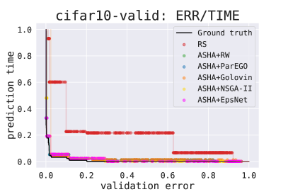
Figure 5: Left: Difference in dominated hypervolume of the Pareto front approximations for the different methods with respect to the optimal Pareto front approximation over time on NAS-201 Cifar-10 dataset with two objectives: ERR and TIME. Right: Pareto fronts found by the different methods on the same dataset.

Figure 6: Objective values visualizing how different methods explore the NAS-201 Cifar-10 architecture space over time. Each model evaluation is represented by a single dot. Darker colors indicate that the model has been evaluated later in time during the search.

Figure 7: Left: Difference in dominated hypervolume of the Pareto front approximations for the different methods with respect to the optimal Pareto front approximation over time on NAS-201 Cifar-100 dataset with two objectives: ERR and TIME. Right: Pareto fronts found by the different methods on the same dataset.

Figure 8: Objective values visualizing how different methods explore the NAS-201 Cifar-100 architecture space over time. Each model evaluation is represented by a single dot. Darker colors indicate that the model has been evaluated later in time during the search.

Figure 9: Left: Difference in dominated hypervolume of the Pareto front approximations for the different methods with respect to the combined front approximation over time on Adult with three objectives: ERR, DSP and DEO. Right: Analog with four objectives: ERR, DSP, DEO and DFP.

Figure 10: Objective values for the exploration of the search space by the different techniques on Wikitext2 dataset under PPL and ERR objectives. Each model evaluation is represented by a single dot, and darker colors indicate that the model has been evaluated later in time during the search.

Figure 11: Left: Difference in dominated hypervolume of the Pareto front approximations for the different methods with respect to the combined front approximation over time on Wikitext2 dataset with two objectives: ERR and TIME. Right: Pareto fronts found by the different methods on the same dataset.

Figure 12: Objective values for the exploration of the search space for the different techniques on Wikitext2 dataset under ERR and TIME objectives. Each model evaluated is represented by a single dot, and darker colors indicate that the model has been evaluated later in time during the search.

Appendix C Comparison with Multi-objective Bayesian Optimization

A recent work [49] evaluated various MBO techniques as well as random search on multiple HPO tasks and artificial functions and investigated the use of multi-fidelity optimization for multi-objective HPO. With Figure 13 we include an excerpt of that study showing dominated hypervolume over time averaged over 5 random seeds for Sklearn MLP optimization on Adult datasets for 2 (ERR, DSP), 3 (ERR, DSP, DEO) and 4 (ERR, DSP, DEO, DFP) objective fairness settings. While [49] allowed the Hyperband methods to use multiple parallel workers we restrict each method to serial execution. One can observe that on these tasks random search can yield comparable sample complexity while causing minimal computational overhead. Unlike GP-based iterative methods, random search is easy to parallelize. Both are desirable properties for HPO algorithms intended to be run on large-scale systems. This motivates the use of multi-fidelity techniques such as Hyperband [36] and ASHA [37] as natural extensions of random search for designing multi-objective HPO algorithms.

Figure 13: Difference in dominated hypervolume of the Pareto front approximations returned by the different methods with respect to the combined front over time on Adult dataset. ERR, DSP, DEO and DFP objective are considered. The average and standard deviation for 5 random seeds is shown. For both scalarization schemes, the Hyperband method obtains Pareto front approximations with larger hypervolume in a shorter wall-clock time compared to multi-objective Bayesian optimization techniques. Random search is surprisingly competitive.

References

- [1] A. Agarwal, A. Beygelzimer, M. Dudik, J. Langford, and H. Wallach. A reductions approach to fair classification. ICML, 2018.
- [2] Syrine Belakaria, Aryan Deshwal, and Janardhan Rao Doppa. Max-value entropy search for multi-objective bayesian optimization. In Advances in Neural Information Processing Systems, pages 7823–7833, 2019.
- [3] Syrine Belakaria, Aryan Deshwal, and Janardhan Rao Doppa. Information-theoretic multi-objective bayesian optimization with continuous approximations. arXiv preprint arXiv:2009.05700, 2020.
- [4] Syrine Belakaria, Aryan Deshwal, and Janardhan Rao Doppa. Multi-fidelity multi-objective bayesian optimization: An output space entropy search approach. In AAAI, pages 10035–10043, 2020.
- [5] Hadjer Benmeziane, Kaoutar El Maghraoui, Hamza Ouarnoughi, Smail Niar, Martin Wistuba, and Naigang Wang. A Comprehensive Survey on Hardware-Aware Neural Architecture Search. pages 1–30, 2021. arXiv: 2101.09336.
- [6] Mickael Binois, Victor Picheny, Patrick Taillandier, and Abderrahmane Habbal. The kalai-smorodinsky solution for many-objective bayesian optimization. Journal of Machine Learning Research, 21(150):1–42, 2020.
- [7] F. Calmon, D. Wei, B. Vinzamuri, K. N. Ramamurthy, and K. R. Varshney. Optimized pre-processing for discrimination prevention. NeurIPS, 2017.
- [8] N. V. Chawla, K. W. Bowyer, L. O. Hall, and W. P. Kegelmeyer. SMOTE: Synthetic minority over-sampling technique. Journal of Artificial Intelligence Research, 2002.
- [9] Stanley F Chen, Douglas Beeferman, and Roni Rosenfeld. Evaluation metrics for language models. 1998.
- [10] Sam Corbett-Davies, Emma Pierson, Avi Feller, Sharad Goel, and Aziz Huq. Algorithmic decision making and the cost of fairness. In Proceedings of the 23rd acm sigkdd international conference on knowledge discovery and data mining, pages 797–806, 2017.
- [11] Kalyanmoy Deb, Amrit Pratap, Sameer Agarwal, and TAMT Meyarivan. A fast and elitist multiobjective genetic algorithm: Nsga-ii. IEEE transactions on evolutionary computation, 6(2):182–197, 2002.
- [12] Xuanyi Dong and Yi Yang. Nas-bench-201: Extending the scope of reproducible neural architecture search. In International Conference on Learning Representations (ICLR), 2020.
- [13] M. Donini, L. Oneto, S. Ben-David, J. S. Shawe-Taylor, and M. Pontil. Empirical risk minimization under fairness constraints. NeurIPS, 2018.
- [14] Thomas Elsken, Frank Hutter, and Jan Hendrik Metzen. Efficient multi-objective neural architecture search via Lamarckian evolution. 7th International Conference on Learning Representations, ICLR 2019, pages 1–23, 2019. arXiv: 1804.09081.
- [15] Michael TM Emmerich, André H Deutz, and Jan Willem Klinkenberg. Hypervolume-based expected improvement: Monotonicity properties and exact computation. In 2011 IEEE Congress of Evolutionary Computation (CEC), pages 2147–2154. IEEE, 2011.
- [16] Michael T.M. Emmerich and André H. Deutz. A tutorial on multiobjective optimization: fundamentals and evolutionary methods. Natural Computing, 17(3):585–609, 2018. ISBN: 0123456789.
- [17] Nick Erickson, Jonas Mueller, Alexander Shirkov, Hang Zhang, Pedro Larroy, Mu Li, and Alexander Smola. Autogluon-tabular: Robust and accurate automl for structured data. arXiv preprint arXiv:2003.06505, 2020.
- [18] M. Feldman, S. A. Friedler, J. Moeller, C. Scheidegger, and S. Venkatasubramanian. Certifying and removing disparate impact. ACM SIGKDD, 2015.
- [19] S. A. Friedler, C. Scheidegger, and S. Venkatasubramanian. On the (im)possibility of fairness. arXiv preprint arXiv:1609.07236, 2016.
- [20] Daniel Golovin and Qiuyi Zhang. Random Hypervolume Scalarizations for Provable Multi-Objective Black Box Optimization. 2020.
- [21] Julia Guerrero-Viu, Sven Hauns, Sergio Izquierdo, Guilherme Miotto, Simon Schrodi, Andre Biedenkapp, Thomas Elsken, Difan Deng, Marius Lindauer, and Frank Hutter. Bag of Baselines for Multi-objective Joint Neural Architecture Search and Hyperparameter Optimization. arXiv:2105.01015 [cs, stat], May 2021. arXiv: 2105.01015.
- [22] M. Hardt, E. Price, and N. Srebro. Equality of opportunity in supervised learning. NeurIPS, 2016.
- [23] José Miguel Henrández-Lobato, Matthew W. Hoffman, and Zoubin Ghahramani. Predictive entropy search for efficient global optimization of black-box functions. In Proceedings of the 27th International Conference on Neural Information Processing Systems - Volume 1, NIPS’14, page 918–926, Cambridge, MA, USA, 2014. MIT Press.
- [24] Daniel Hernández-Lobato, Jose Hernandez-Lobato, Amar Shah, and Ryan Adams. Predictive entropy search for multi-objective bayesian optimization. In International Conference on Machine Learning, pages 1492–1501, 2016.
- [25] José Miguel Hernández-Lobato, Michael A. Gelbart, Ryan P. Adams, Matthew W. Hoffman, and Zoubin Ghahramani. A general framework for constrained bayesian optimization using information-based search. Journal of Machine Learning Research, 17(160):1–53, 2016.
- [26] Kevin Jamieson and Ameet Talwalkar. Non-stochastic best arm identification and hyperparameter optimization. In Artificial Intelligence and Statistics, pages 240–248, 2016.
- [27] Donald R Jones, Matthias Schonlau, and William J Welch. Efficient global optimization of expensive black-box functions. Journal of Global optimization, 13(4):455–492, 1998.
- [28] Andy J Keane. Statistical improvement criteria for use in multiobjective design optimization. AIAA journal, 44(4):879–891, 2006.
- [29] J. Kleinberg. Inherent trade-offs in algorithmic fairness. SIGMETRICS, 2018.
- [30] Jon Kleinberg, Sendhil Mullainathan, and Manish Raghavan. Inherent trade-offs in the fair determination of risk scores. arXiv preprint arXiv:1609.05807, 2016.
- [31] Joshua Knowles. Parego: a hybrid algorithm with on-line landscape approximation for expensive multiobjective optimization problems. IEEE Transactions on Evolutionary Computation, 10(1):50–66, 2006.
- [32] Ron Kohavi. Scaling up the accuracy of naive-bayes classifiers: A decision-tree hybrid. In Kdd, volume 96, pages 202–207, 1996.
- [33] H. J. Kushner. A New Method of Locating the Maximum Point of an Arbitrary Multipeak Curve in the Presence of Noise. Journal of Basic Engineering, 86(1):97–106, 03 1964.
- [34] Yann LeCun. The mnist database of handwritten digits. http://yann. lecun. com/exdb/mnist/, 1998.
- [35] Yann LeCun, Patrick Haffner, Léon Bottou, and Yoshua Bengio. Object recognition with gradient-based learning. In Shape, contour and grouping in computer vision, pages 319–345. Springer, 1999.
- [36] L. Li, K. Jamieson, G. DeSalvo, Afshin Rostamizadeh, and Ameet Talwalkar. Hyperband: A novel bandit-based approach to hyperparameter optimization. J. Mach. Learn. Res., 18:185:1–185:52, 2017.
- [37] Liam Li, Kevin Jamieson, Afshin Rostamizadeh, Ekaterina Gonina, Moritz Hardt, Ben Recht, and Ameet Talwalkar. Massively parallel hyperparameter tuning. 2018.
- [38] Stephen Merity, Caiming Xiong, James Bradbury, and Richard Socher. Pointer sentinel mixture models. arXiv preprint arXiv:1609.07843, 2016.
- [39] Jonas Mockus, Vytautas Tiesis, and Antanas Zilinskas. The application of bayesian methods for seeking the extremum. Towards global optimization, 2(117-129):2, 1978.
- [40] Hirotaka Nakayama, Yeboon Yun, and Min Yoon. Sequential approximate multiobjective optimization using computational intelligence. Springer Science & Business Media, 2009.
- [41] Biswajit Paria, Kirthevasan Kandasamy, and Barnabás Póczos. A flexible framework for multi-objective bayesian optimization using random scalarizations. In UAI, 2019.
- [42] Adam Paszke, Sam Gross, Francisco Massa, Adam Lerer, James Bradbury, Gregory Chanan, Trevor Killeen, Zeming Lin, Natalia Gimelshein, Luca Antiga, Alban Desmaison, Andreas Kopf, Edward Yang, Zachary DeVito, Martin Raison, Alykhan Tejani, Sasank Chilamkurthy, Benoit Steiner, Lu Fang, Junjie Bai, and Soumith Chintala. Pytorch: An imperative style, high-performance deep learning library. In H. Wallach, H. Larochelle, A. Beygelzimer, F. d'Alché-Buc, E. Fox, and R. Garnett, editors, Advances in Neural Information Processing Systems 32, pages 8024–8035. Curran Associates, Inc., 2019.
- [43] F. Pedregosa, G. Varoquaux, A. Gramfort, V. Michel, B. Thirion, O. Grisel, M. Blondel, P. Prettenhofer, R. Weiss, V. Dubourg, J. Vanderplas, A. Passos, D. Cournapeau, M. Brucher, M. Perrot, and E. Duchesnay. Scikit-learn: Machine learning in Python. Journal of Machine Learning Research, 12:2825–2830, 2011.
- [44] Valerio Perrone, Michele Donini, Krishnaram Kenthapadi, and Cédric Archambeau. Fair bayesian optimization. AutoML Workshop - ICML, 2020.
- [45] Victor Picheny. Multiobjective optimization using gaussian process emulators via stepwise uncertainty reduction. Statistics and Computing, 25(6):1265–1280, 2015.
- [46] G. Pleiss, M. Raghavan, F. Wu, J. Kleinberg, and K. Q. Weinberger. On fairness and calibration. NeurIPS, 2017.
- [47] Wolfgang Ponweiser, Tobias Wagner, Dirk Biermann, and Markus Vincze. Multiobjective optimization on a limited budget of evaluations using model-assisted -metric selection. In International Conference on Parallel Problem Solving from Nature, pages 784–794. Springer, 2008.
- [48] D. Salinas, V. Perrone, O. Cruchant, and C. Archambeau. A multi-objective perspective on jointly tuning hardware and hyperparameters. ICLR Workshop on Neural Architecture Search, 2021.
- [49] R. Schmucker, M. Donini, V. Perrone, M. B. Zafar, and C. Archambeau. Multi-objective multi-fidelity hyperparameter optimization with application to fairness. NeurIPS Workshop on Meta-Learning, 2020.
- [50] Nidamarthi Srinivas and Kalyanmoy Deb. Multiobjective optimization using nondominated sorting in genetic algorithms. Evolutionary computation, 2(3):221–248, 1994.
- [51] Emma Strubell, Ananya Ganesh, and Andrew McCallum. Energy and policy considerations for deep learning in NLP. In Proceedings of the 57th Annual Meeting of the Association for Computational Linguistics, pages 3645–3650, Florence, Italy, July 2019. Association for Computational Linguistics.
- [52] Shinya Suzuki, Shion Takeno, Tomoyuki Tamura, Kazuki Shitara, and Masayuki Karasuyama. Multi-objective bayesian optimization using pareto-frontier entropy. arXiv preprint arXiv:1906.00127, 2019.
- [53] Joshua D Svenson and Thomas J Santner. Multiobjective optimization of expensive black-box functions via expected maximin improvement. The Ohio State University, Columbus, Ohio, 32, 2010.
- [54] Mingxing Tan, Bo Chen, Ruoming Pang, Vijay Vasudevan, Mark Sandler, Andrew Howard, and Quoc V. Le. MnasNet: Platform-Aware Neural Architecture Search for Mobile. 2018.
- [55] Ashish Vaswani, Noam Shazeer, Niki Parmar, Jakob Uszkoreit, Llion Jones, Aidan N Gomez, Lukasz Kaiser, and Illia Polosukhin. Attention is all you need. arXiv preprint arXiv:1706.03762, 2017.
- [56] S. Verma and J. Rubin. Fairness definitions explained. FairWare, 2018.
- [57] Tobias Wagner, Michael Emmerich, André Deutz, and Wolfgang Ponweiser. On expected-improvement criteria for model-based multi-objective optimization. In International Conference on Parallel Problem Solving from Nature, pages 718–727. Springer, 2010.
- [58] Zi Wang and Stefanie Jegelka. Max-value entropy search for efficient bayesian optimization. In Proceedings of the 34th International Conference on Machine Learning - Volume 70, ICML’17, page 3627–3635. JMLR.org, 2017.
- [59] Bichen Wu, Xiaoliang Dai, Peizhao Zhang, Yanghan Wang, Fei Sun, Yiming Wu, Yuandong Tian, Peter Vajda, Yangqing Jia, and Kurt Keutzer. FBNET: Hardware-aware efficient convnet design via differentiable neural architecture search. Proceedings of the IEEE Computer Society Conference on Computer Vision and Pattern Recognition, 2019-June:10726–10734, 2019. arXiv: 1812.03443 ISBN: 9781728132938.
- [60] M. B. Zafar, I. Valera, M. Gomez-Rodriguez, and K. P. Gummadi. Fairness constraints: Mechanisms for fair classification. AISTATS, 2017.
- [61] M. B. Zafar, I. Valera, M. Gomez-Rodriguez, and K. P. Gummadi. Fairness constraints: A flexible approach for fair classification. JMLR, 2019.
- [62] R. Zemel, Y. Wu, K. Swersky, T. Pitassi, and C. Dwork. Learning fair representations. ICML, 2013.
- [63] B. H. Zhang, B. Lemoine, and M. Mitchell. Mitigating unwanted biases with adversarial learning. AIES, 2018.
- [64] Qingfu Zhang, Wudong Liu, Edward Tsang, and Botond Virginas. Expensive multiobjective optimization by moea/d with gaussian process model. IEEE Transactions on Evolutionary Computation, 14(3):456–474, 2009.
- [65] Richard Zhang and Daniel Golovin. Random hypervolume scalarizations for provable multi-objective black box optimization. In Hal Daumé III and Aarti Singh, editors, Proceedings of the 37th International Conference on Machine Learning, volume 119 of Proceedings of Machine Learning Research, pages 11096–11105. PMLR, 13–18 Jul 2020.
- [66] Eckart Zitzler and Lothar Thiele. Multiobjective optimization using evolutionary algorithms—a comparative case study. In International conference on parallel problem solving from nature, pages 292–301. Springer, 1998.
- [67] Barret Zoph and Quoc V. Le. Neural architecture search with reinforcement learning, 2017.
- [68] Marcela Zuluaga, Guillaume Sergent, Andreas Krause, and Markus Püschel. Active learning for multi-objective optimization. In International Conference on Machine Learning, pages 462–470, 2013.