Lifting convex inequalities for bipartite bilinear programs
Abstract
The goal of this paper is to derive new classes of valid convex inequalities for quadratically constrained quadratic programs (QCQPs) through the technique of lifting. Our first main result shows that, for sets described by one bipartite bilinear constraint together with bounds, it is always possible to sequentially lift a seed inequality that is valid for a restriction obtained by fixing variables to their bounds, when the lifting is accomplished using affine functions of the fixed variables. In this setting, sequential lifting involves solving a non-convex nonlinear optimization problem each time a variable is lifted, just as in Mixed Integer Linear Programming. To reduce the computational burden associated with this procedure, we develop a framework based on subadditive approximations of lifting functions that permits sequence-independent lifting of seed inequalities for separable bipartite bilinear sets. In particular, this framework permits the derivation of closed-form valid inequalities. We then study a separable bipartite bilinear set where the coefficients form a minimal cover with respect to the right-hand-side. For this set, we introduce a bilinear cover inequality, which is second-order cone representable. We argue that this bilinear cover inequality is strong by showing that it yields a constant-factor approximation of the convex hull of the original set. We study its lifting function and construct a two-slope subadditive upper bound. Using this subadditive approximation, we lift fixed variable pairs in closed-form, thus deriving a lifted bilinear cover inequality that is valid for general separable bipartite bilinear sets with box constraints.
1 Introduction
1.1 Generating strong cutting planes through lifting
Lifting is a technique that is used to derive or strengthen classes of cutting planes. It was first introduced to optimization in the context of mixed integer linear programming (MILP); see [46] for a review. The lifting process has two steps:
-
•
Fixing and generation of a seed inequality: In the first step, the set of interest is restricted by fixing a subset of variables, say , to specific values (typically to one of their bounds), say . A valid inequality , which we call seed inequality, is then generated for the restriction .
-
•
Lifting the seed inequality: The seed inequality , when viewed with “zero coefficients" for the fixed variables is typically not valid for the original set . The task in the lifting step is to generate an inequality , which (i) is valid for and (ii) satisfies . Under condition (ii), inequality reduces to inequality when is set to . The process of lifting is often accomplished by rotating or titling the seed inequality [27].
Though condition (ii) is not strictly necessary to impose, we require it in the remainder of the paper as otherwise is weak on the face .
Lifting, as a technique for generating cutting-planes in MILP, has been extensively researched. Originally devised for node packing and knapsack sets [43, 44, 7, 35, 10], lifting was extended to general settings [54, 55, 31, 32, 47, 48, 4] and used to derive families of valid inequalities for many sets including [19, 38, 3, 1, 36, 22, 56, 57, 58, 28]. Many of the classes of cutting planes that have yielded significant computational gains can be obtained through lifting. This includes lifted cover inequalities [31], lifted tableaux cuts [22, 41], and even the Gomory mixed integer cut [26]; see [9, 50, 25, 21, 12, 11, 13, 6, 14, 24, 13] for papers related to lifting in the infinite group problem model. Similarly, mixing inequalities [33] can be viewed as an outcome of lifting [24].
Significantly fewer articles have focused on studying how lifting can be applied to nonlinear programs and mixed integer nonlinear programs. Exceptions include [51], which develops a general theory for lifting linear inequalities in nonlinear programming, [42] which applies lifting to derive the convex hull of a nonlinear set, [34] which studies lifting for the pooling problem, [5] which uses lifting for conic integer programs, and [20] which develops strong inequalities for mixed integer bilinear programs.
1.2 Goal of this paper
The goal of this paper is to derive new classes of valid convex inequalities for quadratically constrained quadratic programs (QCQPs) through the technique of lifting.
Generating valid inequalities for single row relaxations (together with bounds and integrality restrictions), i.e., for knapsack constraints, was the first, and arguably the most important step in the development of computationally useful cutting-planes in MILP. Motivated by this observation, various cutting-planes and convexification techniques for sets defined by a single non-convex quadratic constraint together with bounds have recently been investigated; see [20, 53, 2] for classes of valid inequalities for single constraint QCQPs and [23, 52] for convex hull results for such sets. The paper [45] studies a set similar to the one we study, albeit with integer variables. Further, [23] demonstrates that cuts obtained from one-row relaxations of QCQPs can be useful computationally. The paradigm of intersection cuts has also been explored to generate cuts for single-constraint QCQPs [40, 16]. Due to lack of space, we refrain from describing here the vast literature on convexification techniques for QCQPs and instead refer interested readers to [18, 52] and the references therein.
In this paper, we investigate the lifting of a convex seed inequality for a feasible region defined by a single (non-convex) quadratic constraint together with bound constraints. Apart from [5], we are not aware of any paper that attempts to study or employ lifting of convex nonlinear inequalities. To the best of our knowledge, this is the first study that derives lifted valid inequalities for general non-convex quadratic constraints with arbitrary number of variables. An extended abstract of this paper was accepted for publication in IPCO 2021 [30].
1.3 Main contributions
-
•
Can we always lift? We present an example in two variables that illustrates that, even when a set is defined by a convex quadratic constraint, it might not always be possible to lift a linear seed inequality, valid for the restriction obtained by fixing a variable at lower bound, when we assume is an affine function of the fixed variable. Our main result, by contrast, establishes that there exists a large class of sets, described by a single bipartite bilinear constraint [23] together with bounds, for which it is always possible to lift when variables are fixed at their bounds. Note that any quadratic constraint can be relaxed to a bipartite bilinear constraint.
-
•
Sequence-independent lifting. The lifting of a fixed variable requires the solution of a non-convex nonlinear optimization problem. When multiple variables must be lifted one at a time, this process (referred to as sequential lifting) can be computationally prohibitive. Further, the form of the lifted inequality obtained will differ depending on the order in which variables are lifted. For MILPs, it was shown in [55] that when the so-called lifting function is subadditive, lifting is far more computationally tractable in part because the form of the lifted inequality is independent of the order in which variables are lifted. We develop a similar general result for sequence-independent lifting of seed inequalities for separable bipartite bilinear constraints.
-
•
Bilinear covering set and bilinear cover inequality. We next study a separable bipartite bilinear set whose coefficients form a minimal cover with respect to the right-hand-side. For this set, we derive a bilinear cover inequality. This second-order cone representable valid inequality yields a constant-factor approximation of the convex hull of the original set.
-
•
Sequence-independent lifting of bilinear cover inequality. We construct a two-slope subadditive upper bound of the lifting function corresponding to the bilinear cover inequality. This function is reminiscent of the two-slope subadditive functions studied in the context of cutting-planes for the infinite group relaxation [29, 49, 37], although there is no apparent connection. Using this subadditive function, we lift fixed variable pairs in closed-form, thus describing a family of lifted bilinear cover inequalities, which are valid for general separable bipartite bilinear constraints.
Notation and organization of the paper
Given a positive integer , we denote the set by . Given a set and , we use to denote the set . We also use to denote the convex hull of set . The rest of the paper is organized as follows. In Section 2 we present our main results. In Section 3 we discuss some key directions for future research. Sections 4-10 give the proofs of the results described in Section 2.
2 Main results
Before we discuss our results, we first present two examples that illustrate how lifting can be performed for a set defined by a quadratic constraint and what challenges can arise during such procedure.
Example 1.
Consider the set First, we fix to obtain the restriction . The seed inequality is a valid convex inequality for . We next show how it can be lifted into a valid inequality for . Observe that, although valid for , the seed inequality is not valid for , since violates it while belonging to . We therefore must introduce variable into the seed inequality so as to make it valid. In particular we seek for which
| (1) |
is valid for . This question can be answered by solving the problem
| (2) |
where a key challenge is to first ascertain that the supremum is finite. When is finite, it is clear that choosing any in (1) yields a valid inequality for . Problem (2) can be analyzed using the following facts: (1) for any fixed value of , we can always assume that an extreme point is the optimal solution, as the objective is to maximize a convex function, and (2) the extreme points of the set where is fixed to a value within its bounds are well-understood [52]. This suggests that one can inspect all different values of to establish that the supremum is finite. We illustrate these calculations next.
Example 1 might suggest that lifting can always be performed when seeking to derive a linear valid inequality. Example 2 shows that it is not so.
Example 2.
Consider the set
The inequality is valid for the set obtained from by fixing . By setting up an optimization problem similar to (2), it is easy to verify that there is no for which is valid for .
In Example 2, () set is convex, () we are trying to lift a linear inequality, and () is fixed to a bound. Even then, it is not possible to lift the seed inequality when we insist that lifting should be accomplished using an affine function of the fixed variable; see Example 4 in Section 3 for further discussion.
2.1 Sufficient conditions under which seed inequalities can be lifted
In Theorem 1, we identify a large class of single row QCQPs where lifting can be accomplished using affine functions of the fixed variables.
Definition 1.
A set is a bipartite bilinear set444We use the term bipartite, perhaps redundantly, to highlight that variables can be divided into two groups, such that any degree two term comes from product of variables one each from these two groups [23]. if it is of the form
where , , , and .
Theorem 1.
Let be a bipartite bilinear set. Given and for , , assume that inequality is valid for , where is a concave function defined on . Then, for any , there exists a finite for which is valid for .
Remark 1.
The proof of Theorem 1 is presented in Section 4 and uses calculations similar to those presented in Example 1. In particular, using a characterization of extreme points of the bipartite bilinear set [23], the proof reduces to establishing the result for three-variable problems where one of the variables is fixed. For a three-variable problem, a number of cases have to be analyzed to verify that the optimal value of an optimization problem similar to (2) is finite. The proof can be turned into an algorithm to compute the lifting coefficients, although not necessarily an efficient or practical one.
Theorem 1 assumes that, when variables and are fixed, they are fixed at their bounds (either or .) When this assumption is not imposed, we show next through an example that lifting may not be possible.
Example 3.
Consider the bipartite bilinear set First, we argue that the seed inequality is valid for the restriction of where . This is clear as when and when . Next, we claim that there is no such that is valid for . Assume by contradiction that is valid for for some . Since , we must have . Since , we must have . This is the desired contradiction as the former expression requires that while the later requires that .
2.2 A framework for sequence-independent lifting
Given a set of variables fixed at their bounds and a seed inequality for the corresponding restriction, a valid inequality for the original problem can be obtained by lifting each fixed variable one at the time. This computationally demanding process requires the solution of a non-convex nonlinear optimization problem, similar to (2), to lift each variable. It results in a lifted inequality whose form depends on the order in which variables are lifted. Next, we study situations where the lifting inequality obtained does not depend on the order in which variables are lifted. In particular, we develop a subadditive theory for lifting in QCQPs that is inspired by that originally developed in MILP in [55]. We consider the special case of separable bipartite bilinear constraints.
Definition 2.
A set is a separable bipartite bilinear set if it is of the form
for some and for , i.e., variables and , for , appear in only one term.
In the separable case, it is natural to lift each pair of variables and together. Next, we derive conditions that guarantee that the form of the lifted inequality obtained is independent of the order in which these pairs are lifted. This result is obtained, as is common in MILP, by deriving a subadditive upper bound on the lifting function of the seed inequality, from which all lifting coefficients can be derived.
Definition 3.
Let be a separable bipartite bilinear set. Assume that is a partition of (i.e., with ) and that , is a valid inequality for . For , we define the lifting function of the seed inequality as
Structured approximations of lifting functions allow for simple lifting of inequalities as described next in Proposition 1, whose proof can be found in Section 5.
Proposition 1.
Let be a separable bipartite bilinear set and let be a partition of . Let be the lifting function of seed inequality for where is a concave function. Assume there exists and concave functions for such that
-
(i)
, ;
-
(ii)
subadditive, (i.e., , ) with ;
-
(iii)
for ,
-
(iv)
for ,
Then, the lifted inequality is a valid convex inequality for .
The statement of Proposition 1 does not specify the type of functional forms to use in ensuring that conditions (iii) and (iv) are satisfied. It is however clear from the definition that choosing to be the concave envelope of over when , and the concave envelope of over when is the preferred choice for .
Remark 2.
While we state the result of Proposition 1 for a set defined by a single separable bipartite bilinear constraint, a similar result would also hold for sets defined by multiple separable bipartite bilinear constraints.
2.3 A seed inequality from a minimal covering set
To generate lifted inequalities for separable bipartite bilinear sets, we focus next on a family of restrictions we refer to as minimal covering sets. For such minimal covering sets, we introduce a provably strong convex, second-order cone representable valid inequality. We use this inequality as the seed in our lifting procedures.
Definition 4.
Let be a positive integer. We say that for form a minimal cover of , if (i) for all , , (ii) , (iii) , . For a separable bipartite bilinear set , we say that a partition of , where , is a minimal cover yielding partition if: for form a minimal cover of . For a minimal cover yielding partition, we let , ; we define and similarly.
Remark 3.
When , conditions (ii) and (iii) in the definition of minimal cover imply condition (i) For example, if for some , then (ii) implies , contradicting (iii). Now (iii) together with for implies .
Notation 1.
Assuming that for form a minimal cover of , we use (i) , (ii) , (iii) , (iv) when , to be any index in such that .
For a minimal cover, conditions (ii) and (iii) in Definition 4 imply that and for all , respectively. Simple computations show that .
Our overall plan is the following. We will fix for and for . Then, we will find a valid seed inequality for the set where the coefficients form a minimal cover. Finally, we will lift this seed inequality. One key reason to generate cuts from a seed inequality corresponding to a minimal cover is the following result.
Theorem 2.
For a nonempty separable bilinear set , either there exists at least one minimal cover yielding partition or is polyhedral.
Loosely speaking, the proof of Theorem 2, which is given in Section 6, is based on showing that if there is no minimal cover yielding partition, then is “almost" a packing-type set, i.e., a set of the form where s are non-negative. For packing sets , [51] shows that where
We say “almost", since there are non-packing sets such as , where there is no partition that yields a minimal cover. Such sets are “overwhelmingly" like a packing set; in the case of the example, it is a perturbation of the packing set . For such sets it is not difficult to show that is polyhedral.
Since the main focus of this paper is the study of lifted convex (nonlinear) inequalities and since in the packing case the convex hull is trivially obtained using McCormick inequalities [39], the remainder of the paper will concentrate on the case where there exists a minimal cover yielding partition.
Associated with a minimal cover is a convex valid inequality that we present next.
Theorem 3.
Consider the separable bipartite bilinear minimal covering set as presented in Definition 2 where , form a minimal cover of . Then, the bilinear cover inequality is valid for :
| (3) |
Our proof of Theorem 3, which is presented in Section 7, uses techniques from disjunctive programming [8] and an “approximate version" of Fourier-Motzkin projection. In particular, using the minimal covering property of the coefficients and a characterization of the extreme points of bipartite bilinear sets [23], we obtain second-order cone representable sets whose union contains all the extreme points separable bipartite bilinear set. Next we write an extended formulation [8, 15] of the convex hull of the union of these sets. Finally, we use the Fourier-Motzkin procedure to project out the auxiliary variables of the extended formulation one at a time. This procedure works to project out most of the variables. The last step however requires a relaxation to be constructed so that projection can be carried in closed-form. Finally we obtain an inequality that is in fact stronger than (3).
Inequality (3) can be viewed as a strengthening of an inequality presented in [53] for the set obtained from by relaxing upper bounds on variables, i.e., where for and . The convex hull of is shown in [53] to be described by nonnegativity constraints together with
| (4) |
The ensuing proposition, whose proof we skip due to lack of space shows that (3) improves on (4). It essentially proceeds by comparing the coefficients of variable pairs inside of the inequalities. Moreover, if and there exists such that , then (3) strictly dominates (4).
Even though Proposition 2 hints at the strength of the bilinear cover inequality, it can be easily verified that (3) does not produce the convex hull of . However there are a number of reasons to use this inequality as a seed for lifting. The first reason is that, not only is inequality (3) second-order cone representable, we only need to introduce one extra variable representing for each , to write it as a second-order cone representable set. Apart from the convenience of using this inequality within modern conic solvers, the main reason for considering it as a seed inequality is its strength. In particular, we prove next that (3) provides a constant factor approximation of the convex hull of the original set.
Theorem 4.
Let be a bipartite bilinear minimal covering set Let . Then
Since is a set of the covering type (that is, its recession cone is the non-negative orthant), we have that . The proof of Theorem 4, which is given in Section 8, is based on optimizing linear functions with non-negative coefficients on and and proving a bound of on the ratio of their optimal objective function values.
2.4 Lifting the bilinear cover inequality
We now follow the framework of Proposition 1 to perform sequence-independent lifting of the bilinear cover inequality. The first step is to study the lifting function.
Theorem 5.
Let be the lifting function for valid inequality (3). Define
| (5) |
where and where if exists and otherwise. Then
-
(i)
,
-
(ii)
is subadditive over with , and
-
(iii)
for .
Although computing the lifting function for an arbitrary valid inequality, in general, appears to be a difficult task, the bilinear cover inequality (3) has sufficient structure that we can derive a strong subadditive upper bound in Theorem 5. The key to proving Theorem 5, as we show in Section 9, is to first obtain the lifting function exactly in a region around the origin, and to argue that the linear upper bound of the lifting function for this region upper bounds the lifting function globally. Figure 1 presents examples of the lifting function , and the upper bound we derived in Theorem 5 for the cases when exists and for the case when it does not.
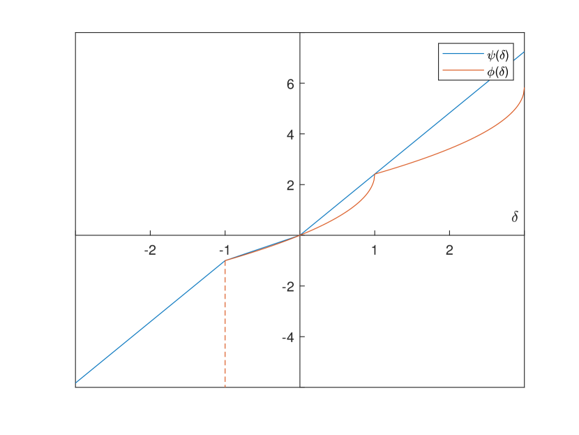
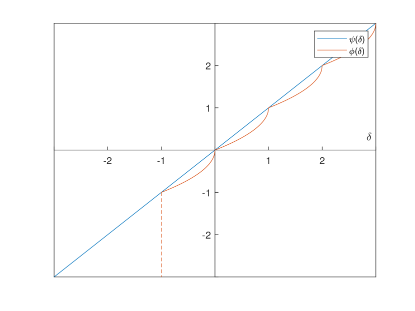
We observe in Figure 1 that the lifting function is not subadditive since it is convex in a neighborhood of the origin. Therefore, building a subadditive approximation is required to achieve sequence-independent lifting.
Building on the subadditive upper bound obtained in Theorem 5, we are now able to lift the bilinear cover inequality in a sequence-independent manner.
Theorem 6.
Consider the separable bipartite bilinear set presented in Definition 2. Let be a minimal cover yielding partition and let be defined as in Theorems 3 and 5 (We clarify that they are calculated using instead of ). Let , , , and, be as in Definition 4. Then inequality
| (6) |
is valid for where for are the concave functions:
-
(i)
for ;
-
(ii)
for ;
-
(iii)
for ;
-
(iv)
for with when , and in all other cases where , with
3 Future directions
The results presented in this paper open up new avenues for generating cutting-planes for QCQPs. They also raise new theoretical and computational questions that can be investigated. To illustrate this assertion, we revisit Example 2 next.
Example 4.
Consider with the same fixing as in Example 2, i.e., . For the associated restriction , consider the seed inequality .
In contrast to our earlier discussion, consider now the problem of lifting this seed inequality into an inequality of the form . Finding the values of that generate a valid inequality is equivalent to solving the problem
Using constraint we can bound the objective function as: It follows that selecting yields a valid inequality for . Note first that leads to an invalid inequality since is a feasible point. Moreover, any yields an invalid inequality, since the point where and is feasible. Therefore, the inequality is the strongest such lifted inequality.
The above example raises the question of obtaining a complete characterization of when one can accomplish lifting, i.e., of generalizing Theorem 1 to situations where the functional form of the lifted variable is not necessarily linear. It would also be valuable to develop a theory to accomplish sequence-independent lifting in the more general case of bipartite bilinear programs, instead of just the separable case. On the computational side, one key question is to understand the complexity of separating the lifted bilinear cover inequality presented in Theorem 6 and to design efficient computational schemes to perform separation. Finally, extensive numerical experiments should be conducted to understand the practical strength of these inequalities and to determine how useful they can be in the solution of QCQPs. Given the strength of the seed inequality, we are hopeful that these lifted inequalities could yield nontrivial dual bound improvements.
4 Proof of Theorem 1
Theorem 1.
Without loss of generality, we assume that we lift a component of the variable , say with . In addition, we assume ; if not we may perform the operation and .
In order to find a lifting coefficient, We examine the following optimization problem
Now note that , assuming it exists, is a valid the coefficient for lifting, i.e., is a valid lifted inequality. Any coefficient larger than is also valid for lifting.
From the concavity of (i.e., convexity of ), for any specific the optimal solution must be an extreme point. According to [23], all extreme points satisfy the following property: except one pair of , all other pairs will be equal to either or . Thus, for any pair of partitions (denoted by ) and (denoted by ), define
We clearly have . In addition, observe that where . Therefore in order to prove that , it is sufficient to show that for any partition , . Therefore, we now focus on one instance of such partitions.
We define and as: , , , In addition, define , , , , and so that we have equivalently
where is after the appropriate restriction. Note that is concave. As we are focusing on the pair of partitions , for simplicity we rewrite the problem as
and . It remains to prove .
For any and , we have
It is clear that for any . Therefore, to show that , it is sufficient to show that . We define
| (0.1) | ||||
| (0.2) | ||||
| (0.3) | ||||
| (0.4) | ||||
| (0.5) | ||||
Denote the feasible region of (7) as . Since (because the seed inequality is assumed to be valid for the restriction), one can prove that by showing that there exists such that
We denote the feasible region of the above problem as .
For , we define to be the optimal value of (7) where constraint is at to equality. We use to denote the corresponding feasible region. For example,
Note that , since the objective function in computing is maximizing a convex function, implying that there exists an optimal solution where at least one of the constraints (0.1)-(0.5) is active.
Thus, to prove that it suffices to show that there exists such that
| (8) |
The case of :
We present a proof of (8) for the case of . The proof is similar for the cases of , , and .
First it is straightforward to verify that there exists a sufficiently small such that for any , we have one of the following two cases: (i) (including the case ) and (ii) , as, for sufficiently small , we may assume that it is impossible that .
-
(i)
We have (this holds even in the case when or ), i.e., .
-
(ii)
We consider two sub-cases:
-
(a)
if , the feasibility of yields . Thus, we have for (actually in case (i).).
-
(b)
if , assume first that . Then . We also denote and since , we have that for .
Since , we have as well as .
Utilizing the fact that (the upper bound from the fact that is assumed to be sufficiently small) and the concavity of , we obtain
(9) We now have
where the second inequality comes from the fact that and , and the third inequality follows from (9), and the last equality follows from Taylor’s series expansion of around .
Thus, there exists such that for . A similar argument holds for the case of .
-
(a)
The case of :
If , then it is easy to see that there always exists an optimal solution to the optimization problem corresponding to computing such that one of (0.1)-(0.4) is active. Therefore if , it is sufficient to verify (8) for , , , and as .
Therefore, we consider the case of for . Without loss of generality assume that or perform the transformation . We in addition assume that or we can scale all parameters by . The problem can now be rewritten as
We denote its feasible region by .
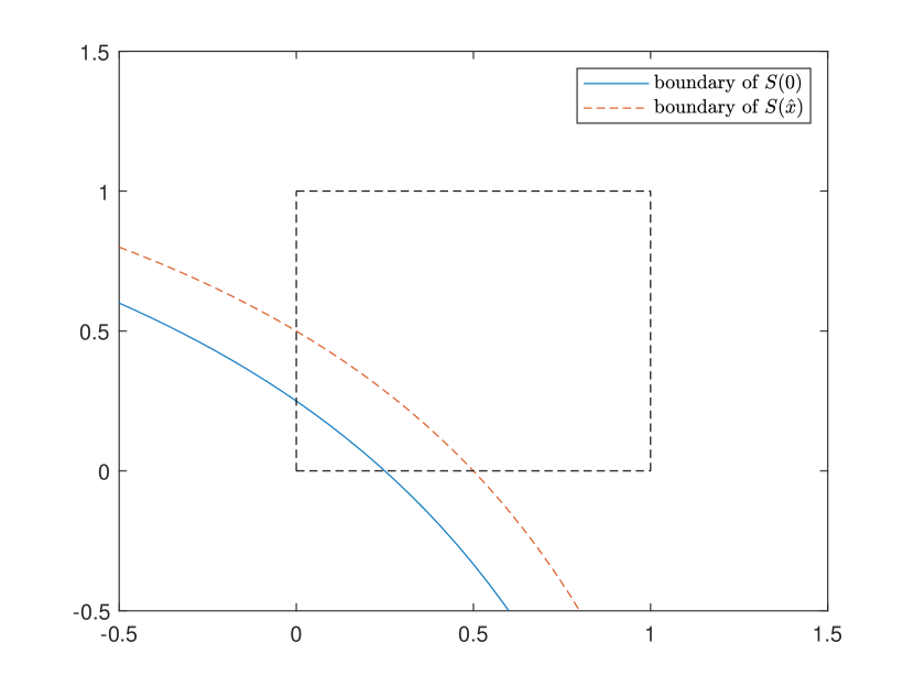
The feasible region is the boundary of a hyperbola intersected with the box. If both the connected components of the hyperbola intersect the box, or , then it is easy to see that there exists an optimal solution of the optimization problem corresponding to computation of where at least one of (0.1)-(0.4) is active, i.e., . So we can disregard this case as well and assume that only one of the connected components of the hyperbola is feasible, as well as .
Note again that if , then there exists such that for all and thus . Therefore we may assume that Let and .
-
(i)
We first consider the case when . Feasibility of requires or . In addition, as only one part of the hyperbola is feasible for for (and sufficiently small), we obtain that either or , and in addition .
-
(a)
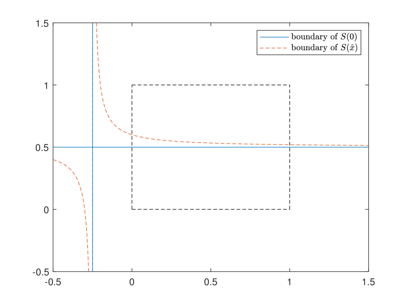
If and (see Fig 2(a)),
as clearly , we have
Thus, depending on the sign of (i.e. sign of for sufficiently small ), for we have, using concavity of , either
or
where is greater than in the first case and is less than in the second. From the continuity of we can get independent of and such that
Therefore, we conclude that
where the second equation comes from the monotonicity of on for sufficiently small , due to the fact that . Since , we have that . Thus, there exists such that for .
-
(b)
If and , a similar analysis can be conducted to obtain such that for .
-
(c)
If or , then so that .
-
(d)
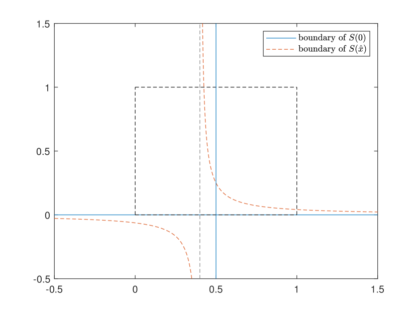
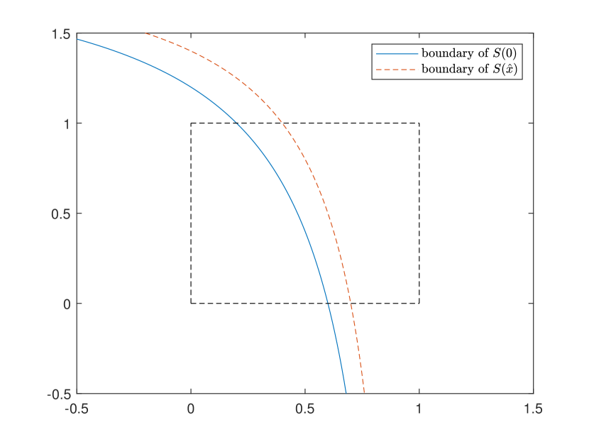
(subcase 1) If with (see Fig 2(b)), we have and (since ). Therefore, for , and for ,
Note that for , using concavity of , we have that
Thus and we obtain such that .
-
(e)
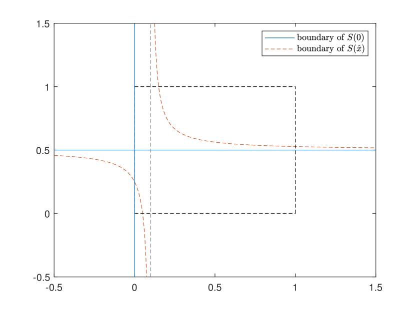
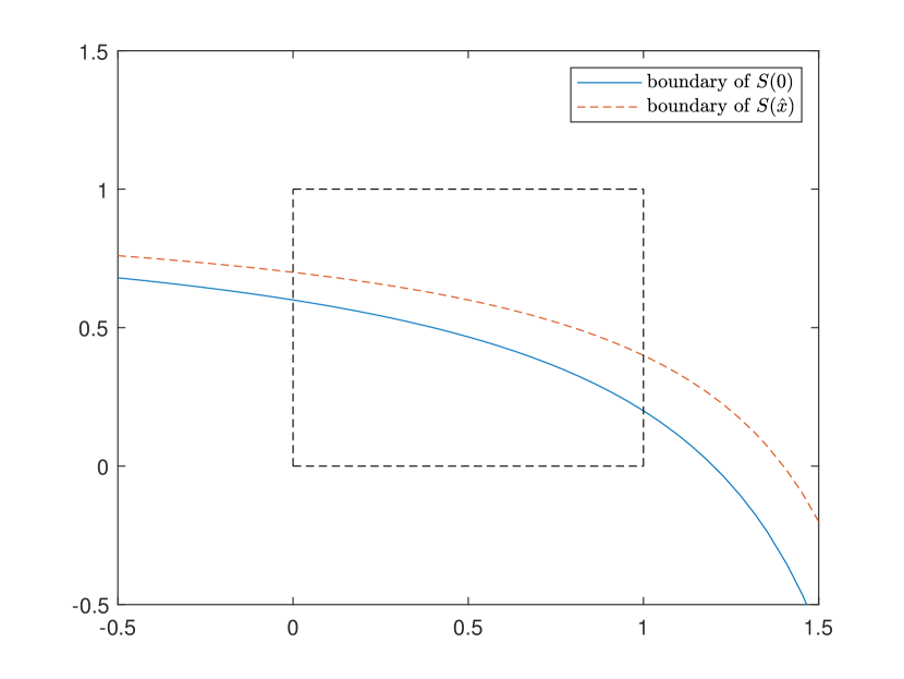
(subcase 1) If with (see Fig 2(c)), we have and . For we have so . For , we have
For , using concavity of , we write
Thus and we get such that .
-
(a)
-
(ii)
We next consider the case when . As discussed above, we assume for all and sufficiently small, and thus . In addition, if for and sufficiently small, we have or but not both.
-
(a)
In the case , for , we denote . Since , we may assume , or . Then clearly and therefore
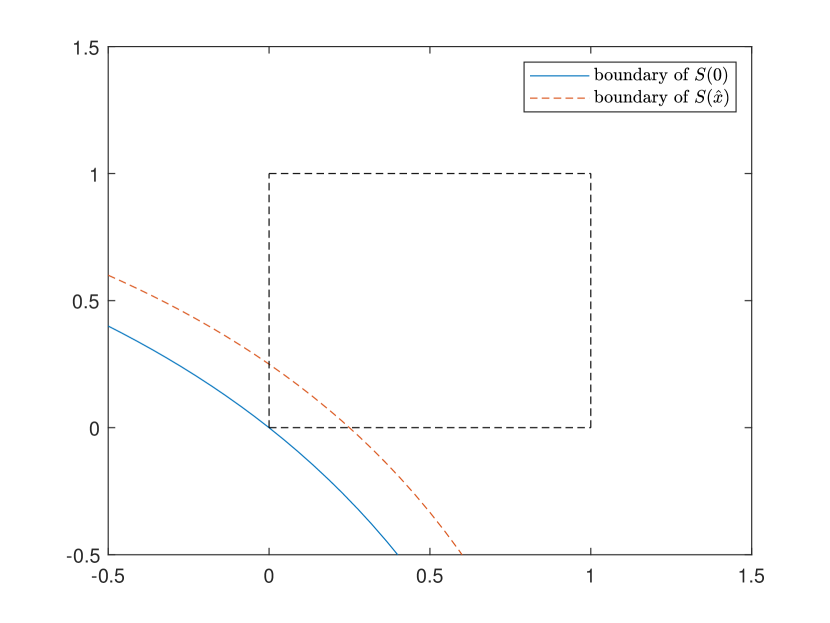
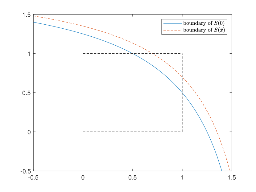
(Subcase 1) If (see Fig 2(d)), we have and . Thus, for , we obtain a curve between and Thus, for any within the curve, from concavity of , it is clear that
where the second inequality uses the concavity of and the fact that for sufficiently small , , and is a constant obtained by taking the derivative of the “max" term times (since , the term is differentiable.) Thus, by setting we have for all sufficiently small .
(Subcase 2) If , but (see Fig 2(e)). Then the curve for is between and . We find such that are within the curve. From the convex nature of one part of the hyperbola, it can be verified that , Consider and denote , noting that and
where
while noting that if , then .
Note that and thus for and therefore for sufficiently small, we obtain or for any . Thus for ,
while noting that continuity gives independent of , .
Now for the case of we have that
Therefore, there exists independent of such that .
A similar analysis of provides for , where is a constant independent of and .
Finally, we combine the results for and . Since they cover the whole curve with overlapping, we have for .
(Subcase 3) If but (see Fig 2(f)), we apply a similar analysis for with and obtain a constant independent of and . We thus get for .
(Subcase 4) If but (see Fig 2(g)), we apply a similar analysis for with and similarly obtain a constant independent of and .
- (b)
-
(a)
∎
5 Proof of Proposition 1
Proposition 1.
Consider any feasible solution . Then
where the first inequality holds because of assumptions (iii) and (iv), the second inequality holds because assumption (ii) requires to be subadditive over its range, the third inequality holds because assumption (i) requires to be an upper bound on , the equality holds from the definition of , and the last inequality is satisfied because is a feasible solution to the preceding optimization problem. ∎∎
6 Proof of Theorem 2
Theorem 2.
Suppose . It follows from [23] that the extreme points of are such that for all for some .
Assume first that has an extreme point where for some with . Define the partition with , , and . Since , we have . Since , we conclude that is a minimal cover yielding partition.
Assume second that all extreme points are such that for all with . Denote and, for , define
It is clear that . Because, for any , is a polytope [51, Proposition 17], we conclude that is a polytope. ∎∎
7 Proof of Theorem 3
Theorem 3.
For , define
First observe that, because for form a minimal cover, we have that for each . This implies that sets are nonempty. We next argue that where . To this end, consider any extreme point of . Then, [23] shows that there exists a partition of such that for , for and . Because for form a minimal cover, it must be that as otherwise . We conclude that . Since is compact, it follows that . Further, since , it is clear that .
We now use disjunctive programming to obtain an extended formulation of . This formulation introduces convex multipliers and copies of variables for each disjunct . Because disjunct yields constraints for , variables and for can be eliminated from the formulation in favor of . Renaming variables as , we obtain
because the constraint functions of each are positively homogeneous.
Using the fact that , we obtain and . Eliminating these variables from the formulation, we obtain
| (19) |
Because projecting variables from the above formulation seems difficult, we relax the above set by using, for each the following inequality
| (20) |
which holds as where the first inequality is obtained by expanding the square and using the arithmetic-geometry mean inequality . Substituting (20) in (19), we obtain:
| (26) |
Using Fourier-Motzkin to project variables , we obtain together with
which is a convex inequality. Retaining only the first term in the maximum for each pair and multiplying through by yields the weaker convex inequality (3). ∎∎
8 Proof of Theorem 4
In this section, we provide a proof of Theorem 4. We say that is a set of the covering type if whenever , then for all such that . Due to lack of space we skip the proof of the next proposition; see [17] for a similar result.
Proposition 3.
Let and let and be sets of the covering type, such that . If there exists , such that for any , , where and , then
Following Proposition 3, Theorem 4 will be proven if, for all ,
satisfy . To this end, we prove first four ancillary results in Lemmas 1-4.
Assumption 1.
, .
Assumption 1 is without loss of generality as it can always be achieved by renaming variables as , if necessary.
Lemma 1.
For and , define
Then, when . Further, when ,
Proof.
When , it follows from Assumption 1 that . The result holds trivially. For , setting , we write , a problem with linear constraints and a convex objective over . When , is optimal and the result follows as . When , the problem has as unique stationary point over . We conclude that is optimal for the constrained problem. ∎∎
Lemma 2.
Let . Then, .
Proof.
Since an optimal solution to the problem defining can always be chosen among the extreme points of and since the proof of Theorem 3 in Section 7 establishes that extreme points of belong to , we write that . Points of satisfy for and . Since , it suffices to consider solutions that satisfy in the above problem, yielding the result. ∎∎
Rearranging the variables if necessary, assume from now on that As a consequence of this assumption and Lemma 2, we obtain that
| (29) |
Lemma 3.
Let . Then for .
Proof.
When , the result is clear. Assume therefore that . When , we write that , where the inequality holds because . When (or equivalently , we write that , where the last inequality holds because . ∎
Lemma 4.
Assume that satisfies (3), i.e., . Define for . Then (i) for all , (ii) for at most one .
Proof.
We are now ready to give a proof of Theorem 4 that inequality (3) yields strong bounds for optimization problems over .
Theorem 4.
Let be an optimal solution for the relaxation defining and let . From Lemma 4, it is sufficient to consider the following three cases.
First assume that for some . Lemma 4 implies for . Then
where the first inequality holds because of Lemma 3, the second inequality holds because for , the third inequality is because from Lemma 4 and because is monotonically increasing, and the fourth inequality holds because of (29).
Second assume that . Lemma 4 implies that for . Similarly,
Finally assume that for all , and we use the same proof as just given. ∎∎
9 Proof of Theorem 5
In this section, we provide a proof of Theorem 5, which gives a subadditive over-approximation to the lifting function of the minimal covering inequality. We first pose
Assumption 2.
.
Assumption 2 can always be achieved by reordering the variables since the notion of minimal cover requires that for ; see discussion following Notation 1.
We next present ancillary results in Lemmas 5-9 and Proposition 4 that are used in the derivation of the approximation of the lifting function. The proof of Lemma 5 is straightforward and can be obtained by investigating signs of derivatives.
Lemma 5.
For where , the function is decreasing when and increasing when .
Lemma 6 establishes that the lifting function exhibits local convexity.
Lemma 6.
Any point of the lifting function corresponding to an optimal solution with at least one index such that , is locally convex, i.e., there exists and such that for all .
Proof.
Let be a point for which an optimal solution () to the problem defining is such that . Define . Consider and construct so that , for any and . From the feasibility of for , we conclude that is a feasible solution to the optimization problem defining . Therefore,
where the last inequality holds because and because the concavity of the square root function over implies that . ∎∎
To obtain the tightest linear over-approximation of for , we next narrow down the set of points where function can achieve a local maximum.
Proposition 4.
Assume that is a local maximizer of the function and that is an optimal solution to the problem defining . Then either
-
(i)
all pairs belong to , or
-
(ii)
there exists such that for all .
Proof.
Assume that (i) does not hold, i.e., there exists for which . We show that (ii) holds. From Lemma 6, there exists and such that for . Without loss of generality, we assume . We consider two cases. Assume first that . For any we have or equivalently . Assume second that . For any we have or equivalently . From analyzing these cases, we see that can be a local maximum only if and all points in are also local maxima. ∎∎
We now derive a linear over-approximation to the function for .
Lemma 7.
Define if and otherwise. Then for .
Proof.
The result holds trivially for since . Our main tool to prove this result is Proposition 4 which will allow us to verify the value of only for a finite set of values of . However, since Proposition 4 holds only for , we first prove the result in an interval that has as an end point.
As mentioned above, the first part of the proof investigates the function in a neighborhood of the point . There are two cases to consider.
For the first case, assume that . Consider . Because the problem defining consists of maximizing a convex function, optimal solutions can be found at extreme points of the feasible region. It follows that there exists an optimal solution that is such that for all for some .
Further, at most one index can be such that as otherwise which would made this solution infeasible for the problem defining .
Also, if there exists with , then . If not, and thus , infeasible. Thus, , i.e., , and as , we obtain
where the last step follows from Lemma 5. Note that is well-defined and convex on . Therefore, it is easy to verify that for , and thus for .
If there is no with , we can verify and . Thus,
where the last step follows Lemma 5. The function is again convex. Therefore, it is easy to verify that for . Thus we obtain that for .
For the second case , i.e., . Note that in this case . Consider . Similar to above, there exists an optimal solution that is such that for all for some . In addition, there exists exactly one index with , or otherwise we obtain a contradiction to . As and , we obtain
The second part of the proof investigates the function away from the origin. As we are attempting to show that bounded from above by , it is sufficient to consider all local maximas of . It follows from Proposition 4 that it is sufficient to verify the condition at values of such that for . (This is because, at other local maximas, the function is locally constant and so it is sufficient to check at the end points of these “constant intervals" where .) Any such local maximum is therefore such that there exists with for and for . We denote it as . It is easily verified that . Let such that , and we have
Consider two cases. On the one hand, if , then and . Thus,
where the inequality follows from the fact that is decreasing on for , and the second last equality holds because .
On the other hand, if , then we have for any . Thus
| ∎ |
∎
Next, we derive an over-approximation of when .
Lemma 8.
Define . For , we have
Further, for .
Proof.
When , as the right-hand-side of the problem defining is larger than . Consider therefore the case when . There exists an optimal solution of the problem defining that is such that for all for some . Further, . We obtain
where the last step follows from Lemma 5. Finally, observe that is convex in . Therefore, by taking a linear inequality tight at and , we obtain that since and . ∎∎
By combining Lemmas 7 and 8, we obtain the following over-approximation of :
Note that the function is not subadditive. Lemma 9 describes a subadditive function that upper bounds , thus giving a subadditive upper bound of .
Lemma 9.
It holds that . Further, the function
is subadditive.
Proof.
Define when and when . Function satisfies and is subadditive since it is straightforward to verify that . Thus, for , such that , we already have that . It remains to consider the cases where at least one of , or belongs to . We do so by considering the possible values of and by assuming without loss of generality that . We use the fact that for , . There are three cases to consider. First assume that . In this case, . Second assume that . In this case, and so that Third assume that . There are two subcases. If , we have If , then . Therefore ∎∎
10 Proof of Theorem 6
Theorem 6.
Following Theorems 3 and 5, it is sufficient to show that for and for , where is the subadditive over-approximation of derived in Theorem 5. We discuss the possible cases.
-
(i)
Assume . We must find for where the equality holds as . As is the best concave upper bound for , we choose .
-
(ii)
Assume . We must find for where the equality holds since . As is the best convex lower bound for , we choose .
-
(iii)
Assume . We must find for . As , .
-
(iv)
Assume . In this case, we must find for . Since , Similar to (iii), we have , and . Thus, is a concave upper bound of .
Next we improve this upper bound when . As and (defined in Theorem 6) are concave, it remains to show the following:
Claim 1.
For , for .
Observe that
Consider first the function :
-
•
:
-
•
: we simply prove for . To this end, we verify: (i) and (ii) . This is sufficient since is a concave function and is a linear function. The proof of (i) is straightforward. To prove (ii) observe that is equivalent to verifying or equivalently which holds since .
Consider second the function :
-
•
: by construction, .
-
•
: first observe that for , where . Since is concave it is sufficient to verify that . This condition holds as which is equivalent to ∎
-
•
∎
References
- [1] Agostinho Agra and Miguel Fragoso Constantino. Lifting two-integer knapsack inequalities. Math Program , 109(1):115–154, 2007.
- [2] Kurt M. Anstreicher, Samuel Burer, and Kyungchan Park. Convex hull representations for bounded products of variables. arXiv preprint arXiv:2004.07233, 2020.
- [3] Alper Atamtürk. On the facets of the mixed–integer knapsack polyhedron. Math Program , 98(1):145–175, 2003.
- [4] Alper Atamtürk. Sequence independent lifting for mixed-integer programming. Oper Res , 52(3):487–490, 2004.
- [5] Alper Atamtürk and Vishnu Narayanan. Lifting for conic mixed-integer programming. Math Program , 126(2):351–363, 2011.
- [6] Gennadiy Averkov and Amitabh Basu. Lifting properties of maximal lattice-free polyhedra. Math Program , 154(1-2):81–111, 2015.
- [7] Egon Balas. Facets of the knapsack polytope. Math Program , 8(1):146–164, 1975.
- [8] Egon Balas. Disjunctive programming: Properties of the convex hull of feasible points. Discrete Appl Math , 89(1-3):3–44, 1998.
- [9] Egon Balas and Robert G. Jeroslow. Strengthening cuts for mixed integer programs. Eur J Oper Res , 4(4):224–234, 1980.
- [10] Egon Balas and Eitan Zemel. Facets of the knapsack polytope from minimal covers. SIAM J Appl Math , 34(1):119–148, 1978.
- [11] Amitabh Basu, Manoel Campêlo, Michele Conforti, Gérard Cornuéjols, and Giacomo Zambelli. Unique lifting of integer variables in minimal inequalities. Math Program , 141(1-2):561–576, 2013.
- [12] Amitabh Basu, Gérard Cornuéjols, and Matthias Köppe. Unique minimal liftings for simplicial polytopes. Math Oper Res , 37(2):346–355, 2012.
- [13] Amitabh Basu, Santanu S. Dey, and Joseph Paat. Nonunique lifting of integer variables in minimal inequalities. SIAM J Discrete Math , 33(2):755–783, 2019.
- [14] Amitabh Basu and Joseph Paat. Operations that preserve the covering property of the lifting region. SIAM J Optim , 25(4):2313–2333, 2015.
- [15] Aharon Ben-Tal and Arkadi Nemirovski. Lectures on modern convex optimization: analysis, algorithms, and engineering applications. SIAM, 2001.
- [16] Daniel Bienstock, Chen Chen, and Gonzalo Munoz. Outer-product-free sets for polynomial optimization and oracle-based cuts. Math Program , 183:1–44, 2020.
- [17] Merve Bodur, Alberto Del Pia, Santanu S Dey, Marco Molinaro, and Sebastian Pokutta. Aggregation-based cutting-planes for packing and covering integer programs. Math Program , 171(1):331–359, 2018.
- [18] Samuel Burer. A gentle, geometric introduction to copositive optimization. Math Program , 151(1):89–116, 2015.
- [19] Sebastián Ceria, Cécile Cordier, Hugues Marchand, and Laurence A. Wolsey. Cutting planes for integer programs with general integer variables. Math Program , 81(2):201–214, 1998.
- [20] Kwanghun Chung, Jean-Philippe P. Richard, and Mohit Tawarmalani. Lifted inequalities for 0-1 mixed-integer bilinear covering sets. Math Program , 145(1-2):403–450, 2014.
- [21] Michele Conforti, Gérard Cornuéjols, and Giacomo Zambelli. A geometric perspective on lifting. Oper Res , 59(3):569–577, 2011.
- [22] Santanu S. Dey and Jean-Philippe P. Richard. Linear-programming-based lifting and its application to primal cutting-plane algorithms. INFORMS J Comput , 21(1):137–150, 2009.
- [23] Santanu S. Dey, Asteroide Santana, and Yang Wang. New SOCP relaxation and branching rule for bipartite bilinear programs. Optim Eng , 20(2):307–336, 2019.
- [24] Santanu S. Dey and Laurence A. Wolsey. Composite lifting of group inequalities and an application to two-row mixing inequalities. Discrete Optim , 7(4):256–268, 2010.
- [25] Santanu S. Dey and Laurence A. Wolsey. Constrained infinite group relaxations of MIPs. SIAM J Optim , 20(6):2890–2912, 2010.
- [26] Santanu S. Dey and Laurence A. Wolsey. Two row mixed-integer cuts via lifting. Math Program , 124(1-2):143–174, 2010.
- [27] Daniel Espinoza, Ricardo Fukasawa, and Marcos Goycoolea. Lifting, tilting and fractional programming revisited. Oper Res Lett , 38(6):559–563, 2010.
- [28] Andres Gómez. Submodularity and valid inequalities in nonlinear optimization with indicator variables, 2018. Available at Optimization online.
- [29] Ralph E. Gomory and Ellis L. Johnson. Some continuous functions related to corner polyhedra. Math Program , 3(1):23–85, 1972.
- [30] Xiaoyi Gu, Santanu S. Dey, and Jean-Philippe P. Richard. Lifting convex inequalities for bipartite bilinear programs. In Mohit Singh and David P. Williamson, editors, Integer Programming and Combinatorial Optimization - 22nd International Conference, IPCO 2021, Atlanta, GA, USA, May 19-21, 2021, Proceedings, volume 12707 of Lecture Notes in Computer Science, pages 148–162. Springer, 2021.
- [31] Zonghao Gu, George L. Nemhauser, and Martin W. P. Savelsbergh. Lifted flow cover inequalities for mixed 0-1 integer programs. Math Program , 85(3):439–467, 1999.
- [32] Zonghao Gu, George L. Nemhauser, and Martin W. P. Savelsbergh. Sequence independent lifting in mixed integer programming. J Comb Optim , 4(1):109–129, 2000.
- [33] Oktay Günlük and Yves Pochet. Mixing mixed-integer inequalities. Math Program , 90(3):429–457, 2001.
- [34] Akshay Gupte. Mixed integer bilinear programming with applications to the pooling problem. PhD thesis, Georgia Institute of Technology, 2012.
- [35] Peter L. Hammer, Ellis L. Johnson, and Uri N. Peled. Facet of regular 0–1 polytopes. Math Program , 8(1):179–206, 1975.
- [36] Konstantinos Kaparis and Adam N. Letchford. Local and global lifted cover inequalities for the 0–1 multidimensional knapsack problem. Eur J Oper Res , 186(1):91–103, 2008.
- [37] Matthias Köppe and Yuan Zhou. An electronic compendium of extreme functions for the Gomory–Johnson infinite group problem. Oper Res Lett , 43(4):438–444, 2015.
- [38] Alexander Martin and Robert Weismantel. The intersection of knapsack polyhedra and extensions. In International Conference on Integer Programming and Combinatorial Optimization, pages 243–256. Springer, 1998.
- [39] Garth P. McCormick. Computability of global solutions to factorable nonconvex programs: Part i — convex underestimating problems. Math Program , 10(1):147–175, 1976.
- [40] Gonzalo Muñoz and Felipe Serrano. Maximal quadratic-free sets. In International Conference on Integer Programming and Combinatorial Optimization, pages 307–321. Springer, 2020.
- [41] Amar K. Narisetty, Jean-Philippe P. Richard, and George L. Nemhauser. Lifted tableaux inequalities for 0–1 mixed-integer programs: A computational study. INFORMS J Comput , 23(3):416–424, 2011.
- [42] Trang T. Nguyen, Jean-Philippe P. Richard, and Mohit Tawarmalani. Deriving convex hulls through lifting and projection. Math Program , 169(2):377–415, 2018.
- [43] Manfred W. Padberg. On the facial structure of set packing polyhedra. Math Program , 5(1):199–215, 1973.
- [44] Manfred W. Padberg. A note on zero-one programming. Oper Res , 23(4):833–837, 1975.
- [45] Hamidur Rahman and Ashutosh Mahajan. Facets of a mixed-integer bilinear covering set with bounds on variables. J Global Optim , 74(3):417–442, 2019.
- [46] Jean-Philippe P. Richard. Lifting techniques for mixed integer programming. Wiley Encyclopedia of Operations Research and Management Science, 2010.
- [47] Jean-Philippe P. Richard, Ismael R. de Farias Jr, and George L. Nemhauser. Lifted inequalities for 0-1 mixed integer programming: Basic theory and algorithms. Math Program , 98(1-3):89–113, 2003.
- [48] Jean-Philippe P. Richard, Ismael R. de Farias Jr, and George L. Nemhauser. Lifted inequalities for 0-1 mixed integer programming: Superlinear lifting. Math Program , 98(1-3):115–143, 2003.
- [49] Jean-Philippe P. Richard and Santanu S. Dey. The group-theoretic approach in mixed integer programming. In 50 Years of Integer Programming 1958-2008, pages 727–801. Springer, 2010.
- [50] Jean-Philippe P. Richard, Yanjun Li, and Lisa A. Miller. Valid inequalities for MIPs and group polyhedra from approximate liftings. Math Program , 118(2):253–277, 2009.
- [51] Jean-Philippe P. Richard and Mohit Tawarmalani. Lifting inequalities: a framework for generating strong cuts for nonlinear programs. Math Program , 121(1):61–104, 2010.
- [52] Asteroide Santana and Santanu S. Dey. The convex hull of a quadratic constraint over a polytope. SIAM J Optim , 30(4):2983–2997, 2020.
- [53] Mohit Tawarmalani, Jean-Philippe P. Richard, and Kwanghun Chung. Strong valid inequalities for orthogonal disjunctions and bilinear covering sets. Math Program , 124(1-2):481–512, 2010.
- [54] Laurence A. Wolsey. Facets and strong valid inequalities for integer programs. Oper Res , 24(2):367–372, 1976.
- [55] Laurence A. Wolsey. Valid inequalities and superadditivity for 0–1 integer programs. Math Oper Res , 2(1):66–77, 1977.
- [56] Bo Zeng and Jean-Philippe P. Richard. A framework to derive multidimensional superadditive lifting functions and its applications. In International Conference on Integer Programming and Combinatorial Optimization, pages 210–224. Springer, 2007.
- [57] Bo Zeng and Jean-Philippe P. Richard. A polyhedral study on 0–1 knapsack problems with disjoint cardinality constraints: facet-defining inequalities by sequential lifting. Discrete Optim , 8(2):277–301, 2011.
- [58] Bo Zeng and Jean-Philippe P. Richard. A polyhedral study on 0–1 knapsack problems with disjoint cardinality constraints: strong valid inequalities by sequence-independent lifting. Discrete Optim , 8(2):259–276, 2011.
