Parameter dependent finite element analysis for ferronematics solutions

Abstract

This paper focuses on the analysis of a free energy functional, that models a dilute suspension of magnetic nanoparticles in a two-dimensional nematic well. The first part of the article is devoted to the asymptotic analysis of global energy minimizers in the limit of vanishing elastic constant, $\ell\rightarrow 0$ where the re-scaled elastic constant $\ell$ is inversely proportional to the domain area. The first results concern the strong $H^{1}$-convergence and a $\ell$-independent $H^{2}$-bound for the global minimizers on smooth bounded 2D domains, with smooth boundary and topologically trivial Dirichlet conditions. The second part focuses on the discrete approximation of regular solutions of the corresponding non-linear system of partial differential equations with cubic non-linearity and non-homogeneous Dirichlet boundary conditions. We establish (i) the existence and local uniqueness of the discrete solutions using fixed point argument, (ii) a best approximation result in energy norm, (iii) error estimates in the energy and $L^{2}$ norms with $\ell$- discretization parameter dependency for the conforming finite element method. Finally, the theoretical results are complemented by numerical experiments on the discrete solution profiles, the numerical convergence rates that corroborates the theoretical estimates, followed by plots that illustrate the dependence of the discretization parameter on $\ell$.

Keywords: ferronematics, composite system energy optimization, convergence of minimizers, finite element method, error estimates, numerical experiments

1 Introduction

Nematic liquid crystals (NLCs) are classical examples of partially ordered materials that combine fluidity with the directional order of crystalline solids [12]. NLCs have long-range orientational order i.e. there are distinguished material directions, referred to as nematic directors such that the NLC properties are different in different directions e.g. along the directors. The anisotropic or direction-dependent NLC response to incident light and electric fields make them the working material of choice for the multi-billion dollar liquid crystal display (LCD) industry [24]. However, NLC devices largely rely on their dielectric anisotropy i.e. the NLC response to external electric fields depends on whether the electric field is parallel or non-parallel to the nematic directors [12]. NLC devices rarely use external magnetic fields since the magnetic anisotropy is typically much smaller than the NLC dielectric anisotropy, so that NLC responses to external magnetic fields are very weak [5]. In the 1970’s, Brochard and de Gennes [5] proposed that a suspension of magnetic nanoparticles in a nematic host could generate a spontaneous magnetization at room temperature, without any external field, substantially enhancing the NLC responses to external magnetic fields. These composite systems have been labelled as ferronematics in the literature. In 2013, Mertelj et al. [30] experimentally designed stable ferronematic suspensions using barium hexaferrite (BaHF) magnetic nanoplatelets in pentylcyano-biphenyl (5CB) liquid crystals. In ferronematic suspensions, the nematic director is coupled to the suspended magnetic nanoparticles through surface interactions, so that the nematic director influences the magnetic moments of the nanoparticles and vice-versa. In fact, this nemato-magnetic coupling induces averaged orientations of the suspended nanoparticles, leading to a spontaneous magnetization, in addition to the ambient nematic order. Consequently, this nemato-magnetic coupling strongly enhances the optical and magnetic responses of this composite system, making them attractive for novel display devices, sensors [9], telecommunications [29], and potentially pharmaceutical applications too.

In this paper, we model a dilute suspension of magnetic nanoparticles in a NLC-filled two-dimensional (2D) domain, with tangent boundary conditions. The tangent boundary conditions require the nematic directors to be tangent to the boundary e.g. for a square domain, the director is tangent to the square edges, naturally creating some sort of mismatch or discontinuity at the square vertices with two intersecting edges. The domain is typically on the micron scale, and the volume fraction of the suspended nanoparticles is small such that the distance between the nanoparticles is usually large compared to the typical nanoparticle size. In the dilute limit, one does not see the individual nanoparticles or the interactions between pairs of nanoparticles, but rather the entire suspension is modelled as a single system with two order parameters: a reduced Landau-de Gennes $\mathbf{Q}$-tensor order parameter with two independent components and a magnetization vector, $\mathbf{M}:=(M_{1},M_{2})$ which models the induced spontaneous magnetization of the suspended nanoparticles [3]. This reduced approach works well for thin NLC systems i.e. NLCs confined to a shallow three-dimensional (3D) system, with a 2D cross-section, such that the height is much smaller than the cross-sectional dimensions [17], with tangent boundary conditions on the bounding surfaces.

Here $\mathbf{Q}\in\mathbf{S}_{0}:=\{\mathbf{Q}=(Q_{ij})_{1\leq i,j\leq 2}\in\mathbb{M}^{2\times 2}:\mathbf{Q}=\mathbf{Q}^{T},\text{tr}\mathbf{Q}=0\},$ where $\displaystyle\mathbf{Q}:=s(2\mathbf{n}\otimes\mathbf{n}-\textit{I})$. The nematic director in the plane is a 2D unit-vector, $\mathbf{n}:=(\cos\theta,\sin\theta),$ where $\theta(x,y)$ is the director angle, that models the preferred in-plane direction of the NLC molecules. The scalar order parameter ${}^{\prime}s(x,y)^{\prime}$ measures the degree of order about $\mathbf{n}$, so that the zero set of $s$ is identified with the set of planar nematic defects, and $I$ is a $2\times 2$ identity matrix. The independent component of $\mathbf{Q}$ are given by $Q_{11}=s\cos 2\theta$ and $Q_{12}=s\sin 2\theta.$ Building on the work in [3], [6], [7], [20], the free energy of this dilute suspension of magnetic nanoparticles in a NLC-filled square well is given by

$$E\left[\mathbf{Q},\mathbf{M}\right]:=\int_{\Omega}\big{(}\frac{K}{2}\left|\nabla\mathbf{Q}\right|^{2}+\frac{A}{2}|\mathbf{Q}|^{2}+\frac{C}{4}|\mathbf{Q}|^{4}\big{)}\,{\rm dx}$$

$$+\int_{\Omega}\big{(}\frac{\kappa}{2}\left|\nabla\mathbf{M}\right|^{2}+\frac{\alpha}{2}|\mathbf{M}|^{2}+\frac{\beta}{4}|\mathbf{M}|^{4}\big{)}~{}\,{\rm dx}$$

$$-\int_{\Omega}\frac{\gamma\mu_{0}}{2}\mathbf{M}^{T}\mathbf{Q}\mathbf{M}~{}\,{\rm dx},$$ (1.1)

where $\Omega$ is a 2D domain with characteristic length $L$ microns, $K$ and $\kappa$ are the nematic and magnetic stiffness constants respectively, $A$ is the re-scaled temperature as is $\alpha$, $C$ and $\beta$ are positive material-dependent constants and $\gamma\mu_{0}$ is the nemato-magnetic coupling parameter. Working at low temperatures requires $A$ and $\alpha$ to be negative, as has been done in this manuscript. The first line is the reduced 2D Landau-de Gennes NLC free energy, the second line is the magnetic energy and the third line is the nemato-magnetic coupling energy. The Dirichlet energy density of $\mathbf{M}$ is introduced to penalize arbitrary rotations between $\mathbf{M}$ and $-\mathbf{M}$, and can be viewed as a regularization term. Some authors argue that this term should be discarded for dilute suspensions but we retain it for the well-posedness of the associated variational problems. Further, if $\gamma>0$, then the coupling energy coerces $\mathbf{n}\cdot\mathbf{M}\approx\pm 1$ whereas if $\gamma<0$, then the coupling energy coerces $\mathbf{n}\cdot\mathbf{M}\approx 0$ almost everywhere. Using the re-scalings as in [3] and [20] and assuming that $\frac{K}{|A|}=\frac{\kappa}{|\alpha|}$ (an idealised assumption for analytical convenience), the ferronematic free energy reduces to

$$\mathcal{E}(\mathbf{Q},\mathbf{M}):= \int_{\Omega}\frac{1}{2}(\left\lvert\nabla Q_{11}\right\rvert^{2}+\left\lvert\nabla Q_{12}\right\rvert^{2}+\left\lvert\nabla M_{1}\right\rvert^{2}+\left\lvert\nabla M_{2}\right\rvert^{2})\,{\rm dx}+\frac{1}{\ell}\int_{\Omega}f_{B}(\mathbf{Q},\mathbf{M})\,{\rm dx},$$ (1.2)

where the re-scaled domain $\Omega$ has unit characteristic length, and $\ell=\frac{K}{|A|L^{2}}$ depends on the nematic elastic constant, temperature and domain size $L$. The first integral is the elastic energy of $\mathbf{Q}$ and $\mathbf{M}$ whereas $f_{B}$ is the quartic bulk energy density given by:

$$f_{B}(\mathbf{Q},\mathbf{M}):=\frac{1}{4}(Q_{11}^{2}+Q_{12}^{2}-1)^{2}+\frac{1}{4}(M_{1}^{2}+M_{2}^{2}-1)^{2}-\frac{c}{2}\big{(}Q_{11}(M_{1}^{2}-M_{2}^{2})+2Q_{12}M_{1}M_{2}\big{)}$$ (1.3)

where the coupling parameter, $c=\frac{\gamma\mu_{0}}{|A|}\sqrt{\frac{C}{2|A|}}\frac{|\alpha|}{\beta}.$ In other words, the sign of $c$ is determined by the sign of $\gamma$ and has the same implications for the nemato-magnetic coupling as $\gamma$. For any $\mathbf{Q}:=(Q_{11},Q_{12})$ and $\mathbf{M}:=(M_{1},M_{2})$, the admissible space is, $\mathcal{A}:=\{\Psi:=(Q_{11},Q_{12},M_{1},M_{2})\in\mathbf{H}^{1}(\Omega)|\,\Psi=\mathbf{g}\text{ on }\partial\Omega\},$ with $\mathbf{H}^{1}(\Omega):=({H}^{1}(\Omega))^{4}$ and a given Dirichlet boundary condition $\mathbf{g}$ (see Section 2). The existence of the global energy minimizers of $\mathcal{E}$ in the admissible space follows from a direct method in the calculus of variations; [15, Section 8.2] the crucial facts are that the admissible space is non-empty; the energy functional $\mathcal{E}$ is coercive and convex in gradient of the variables $(Q_{11},Q_{12},M_{1},M_{2})$. Setting $\tilde{Q}:=\textit{Q}_{11}^{2}+\textit{Q}_{12}^{2}-1,$ $\tilde{M}:=M_{1}^{2}+M_{2}^{2}-1$, the corresponding Euler-Lagrange equations are given by

$$\Delta\textit{Q}_{ij}-\ell^{-1}(\widetilde{Q}\textit{Q}_{ij}-c(M_{i}M_{j}-\delta_{ij}\left\lvert M\right\rvert^{2}/2))=0\text{ and }\Delta M_{i}-\ell^{-1}(\widetilde{M}M_{i}-c\textit{Q}_{ij}M_{j})=0,\quad i,j=1,2.$$ (1.4)

When $c=0$, the ferronematic free energy simply reduces to the celebrated Ginzburg-Landau free energy for superconductors [2]. This is a very well-studied problem, and arises naturally in reduced 2D Landau-de Gennes descriptions of confined NLCs [17]. From a purely analytic point of view, this 2D problem has been addressed in a batch of papers [21], [37] etc. where the authors analyse the reduced minimizers on 2D polygons and obtain powerful results on the multiplicity of minimizers, the dimensionality, structure and locations of the corresponding defect sets and bifurcations as a function of the domain size. In [26], the authors study the reduced 2D NLC model on square domains and numerically compute the solution branches using finite element methods, investigating the effect of surface anchoring effects on the energy minimizers. An a priori and a posteriori error analysis for Nitsche’s and the discontinuous Galerin methods have been analyzed for the reduced model (with $c=0$) [33, 27]. A structure-preserving finite element method for the computation of equilibrium configurations, when the $\mathbf{Q}$ is constrained to be uniaxial in 3D, has been proposed in [4], and the stability and consistency of this method without regularization, and $\Gamma$-convergence of the discrete energies to the continuous solutions, in the limit of vanishing mesh size, is studied. The reader is referred to [36] for a detailed survey of the mathematical models of liquid crystals and the developments of numerical methods to find liquid crystal configurations.

For ferronematic systems with $c\neq 0$, the volume of work is limited. In [10], the authors analyze a dilute ferronematic suspension in a one-dimensional channel geometry with Dirichlet boundary conditions for both $\mathbf{Q}$ and $\mathbf{M}$. The authors derive some key analytic ingredients - existence theorems, uniqueness theorems, maximum principle arguments and symmetric solution profiles. They also compute bifurcation diagrams for the solution branches as a function of $\ell$ and $c$. In 2D, there is fairly elaborate numerical work in [3] and [20] where the authors numerically compute stable ferronematic equilibria on 2D polygons with tangent boundary conditions. They report the co-existence of stable equilibria with magnetic domain walls, and stable equilibria with pairs of interior NLC defects, again paying attention to the effects of $\ell$ and $c$. In particular, there are two distinguished limits: the $\ell\to\infty$ limit for small nano-scale systems which admits a unique equilibrium, and the $\ell\to 0$ limit for large micron-scale systems with multiple stable equilibria. Their numerical results suggest that positive $c$ suppresses multistability whereas negative $c$ strongly enhances multistability for applications.

There has been little, if any, analytic and numerical analysis for 2D ferronematic systems, to the best of our knowledge. The main contributions of this paper are: (i) asymptotic analyses of minimizers of the ferronematic free energy on smooth 2D domains, with smooth boundaries and topologically trivial Dirichlet conditions in the $\ell\to 0$ limit and (ii) an a priori finite element error analysis for the discrete approximation of the solutions of the corresponding Euler-Lagrange equations and (iii) relevant numerical experiments to tie the asymptotic analysis and finite element analysis. The asymptotic analysis includes a strong convergence result of the global energy minimizers to minimizers of the bulk energy density in $H^{1}$, and an uniform convergence of the global energy minimizers to the limiting maps, as $\ell\rightarrow 0$, which follows from a non-trivial Bochner inequality for the ferronematic free energy density. The Bochner inequality allows us to prove a $\ell$-independent $H^{2}$-bound for global energy minimizers in this limit. The $H^{2}$-bound is subsequently exploited in the finite element analysis, and the key results are: (i) an elegant representation of the non-linear operator corresponding to the coupled system of partial differential equations (PDEs) (1.4) with cubic and quadratic non-linear lower order terms and non-homogeneous boundary datum; (ii) a finite element convergence analysis that includes the existence and uniqueness of discrete solutions approximating the regular solutions of (1.4) for which $\ell$-independent $H^{2}$-bound hold, a best approximation result in energy norm, optimal convergence rates of $\mathcal{O}(h)$ and $\mathcal{O}(h^{2})$ in energy and $L^{2}$ norms, respectively, for a sufficiently small choice of the discretization parameter (denoted by $h$) which depends on $\ell$ and (iii) numerical results for discrete solution landscapes with positive and negative $c$, order of convergence in energy and $L^{2}$ norms, and numerical errors as a function of $\ell$ and $h$.

Throughout the paper, standard notations on Sobolev spaces and their norms are employed. The standard semi-norm and norm on $H^{s}(\Omega)$ $(\text{resp.}\,W^{s,p}(\Omega))$ for $s,p$ positive real numbers, are denoted by $\left\lvert\cdot\right\rvert_{s}$ and ${|\kern-1.07639pt|\cdot|\kern-1.07639pt|}_{s}$ $(\text{resp. }\left\lvert\cdot\right\rvert_{s,p}\text{ and }{|\kern-1.07639pt|\cdot|\kern-1.07639pt|}_{s,p})$. The standard $L^{2}(\Omega)$ inner product is denoted by $(\cdot,\cdot)$. We use the notation $\mathbf{H}^{s}(\Omega)$ (resp. $\mathbf{L}^{p}(\Omega)$) to denote the product space $(H^{s}(\Omega))^{4}$ $(\text{resp. }(L^{p}(\Omega))^{4}.$ The standard norms ${|\kern-1.07639pt|\kern-1.07639pt|\cdot|\kern-1.07639pt|\kern-1.07639pt|}_{s}$ ($\text{resp. }{|\kern-1.07639pt|\kern-1.07639pt|\cdot|\kern-1.07639pt|\kern-1.07639pt|}_{s,p}$) in the Sobolev spaces $\mathbf{H}^{s}(\Omega)$ ($\text{resp. }\mathbf{W}^{s,p}(\Omega)$) and defined by ${|\kern-1.07639pt|\kern-1.07639pt|\Phi|\kern-1.07639pt|\kern-1.07639pt|}_{s}\!=(\sum_{i=1}^{4}{|\kern-1.07639pt|\varphi_{i}|\kern-1.07639pt|}_{s}^{2})^{\frac{1}{2}}$ for all $\Phi\!=\!(\varphi_{1},\varphi_{2},\varphi_{3},\varphi_{4})\in\!\mathbf{H}^{s}(\Omega)$ $(\text{resp. }{|\kern-1.07639pt|\kern-1.07639pt|\Phi|\kern-1.07639pt|\kern-1.07639pt|}_{s,p}\!\!=(\sum_{i=1}^{4}{|\kern-1.07639pt|\varphi_{i}|\kern-1.07639pt|}_{s,p}^{2})^{\frac{1}{2}}$ for all $\Phi\!=\!(\varphi_{1},\varphi_{2},\varphi_{3},\varphi_{4})\!\in\!\mathbf{W}^{s,p}(\Omega)).$ The norm on $\mathbf{L}^{2}(\Omega)$ space is defined by ${|\kern-1.07639pt|\kern-1.07639pt|\Phi|\kern-1.07639pt|\kern-1.07639pt|}_{0}\!=(\sum_{i=1}^{4}{|\kern-1.07639pt|\varphi_{i}|\kern-1.07639pt|}_{0}^{2})^{\frac{1}{2}}$ for all $\Phi\!=\!(\varphi_{1},\varphi_{2},\varphi_{3},\varphi_{4})\in\!\mathbf{L}^{2}(\Omega).$ Set $V:=H_{0}^{1}(\Omega),$ $\,\!\mathbf{V}:=\mathbf{H}_{0}^{1}(\Omega)=(H_{0}^{1}(\Omega))^{4}$, and $X:=H^{1}(\Omega),\,\mathbf{X}:=\mathbf{H}^{1}(\Omega)$. Throughout this paper, $C$ will denote a generic constant which will always be independent of $\ell$ and the mesh parameter $h$. Define the trace spaces $\mathbf{H}^{m-\frac{1}{2}}(\partial\Omega):=\{\mathbf{w}|_{\partial\Omega}:\mathbf{w}\in\mathbf{H}^{m}(\Omega)\}$ for $m=1,2,$ and $\mathbf{H}^{-\frac{1}{2}}(\partial\Omega):=(\mathbf{H}^{\frac{1}{2}}(\partial\Omega))^{*}$ equipped with the norm $\displaystyle{|\kern-1.07639pt|\kern-1.07639pt|\mathbf{q}|\kern-1.07639pt|\kern-1.07639pt|}_{m-\frac{1}{2},\partial\Omega}:=\inf_{\begin{subarray}{c}\mathbf{w}\in\mathbf{H}^{m}(\Omega)\\ \mathbf{w}|_{\partial\Omega}=\mathbf{q}\end{subarray}}{|\kern-1.07639pt|\kern-1.07639pt|\mathbf{w}|\kern-1.07639pt|\kern-1.07639pt|}_{m}$ and $\displaystyle{|\kern-1.07639pt|\kern-1.07639pt|\mathbf{q}|\kern-1.07639pt|\kern-1.07639pt|}_{-\frac{1}{2},\partial\Omega}:=\sup_{\begin{subarray}{c}\mathbf{k}\in\mathbf{H}^{\frac{1}{2}}(\partial\Omega)\\ \mathbf{k}\neq 0\end{subarray}}\frac{\langle\mathbf{q},\mathbf{k}\rangle_{\partial\Omega}}{{|\kern-1.07639pt|\kern-1.07639pt|\mathbf{k}|\kern-1.07639pt|\kern-1.07639pt|}_{\frac{1}{2},\partial\Omega}}$, respectively. Also, the operator norm for $\mathbf{f}\in\mathbf{L}^{2}(\Omega)$ is defined as $\displaystyle{|\kern-1.07639pt|\kern-1.07639pt|\mathbf{f}|\kern-1.07639pt|\kern-1.07639pt|}_{\mathbf{L}^{2}}:=\sup_{\begin{subarray}{c}\mathbf{v}\in\mathbf{L}^{2}(\Omega)\\ \mathbf{v}\neq 0\end{subarray}}\frac{(\mathbf{f},\mathbf{v})_{\Omega}}{{|\kern-1.07639pt|\kern-1.07639pt|\mathbf{v}|\kern-1.07639pt|\kern-1.07639pt|}_{0}}$.

The paper is organized as follows. Section 2 focuses on the asymptotic analysis of global energy minimizers in the $\ell\to 0$ limit. Section 3 discusses the finite element convergence analysis of the discrete solutions of (1.4). The conforming finite element formulation of the problem is derived and the a priori estimates are proven in Section 3.4. The article concludes with several numerical results for the discrete solutions, and the convergence history for various values of $\ell$, $c$ and $h$ in Section 4.

2 Asymptotic analysis of the minimizers

The primary goal of this section is to establish ${H}^{2}$-bound for the global energy minimizers independent of $\ell,$ in the $\ell\to 0$ limit, under suitable assumptions on the domain and boundary conditions. The $\ell\to 0$ limit is relevant for macroscopic domains or large domains, that are much larger than characteristic material-dependent and temperature-dependent nematic and magnetic correlation lengths [3]. The proof is done in several stages: analysis of the minimizers of the bulk potential reproduced from [10], a strong convergence result for global minimizers followed by convergence results for the bulk potential that largely follow from [2], followed by a delicate Bochner inequality for the energy density that combines ideas from [2] and [16]. Once we have the Bochner inequality, the $\ell$-independent ${H}^{2}$-bound for global energy minimizers in the $\ell\to 0$ limit is relatively standard, from estalished techniques in the Ginzburg-Landau theory for superconductivity although additional technical difficulties are encountered due to the four degrees of freedom in the problem.

Lemma 2.1 (Global minimizers of $f_{B}$).

The bulk potential $f_{B}$ in (1.3) is coercive. For $c>0,$ $f_{B}$ attains its minimum at $\Psi^{\min}:=(Q_{c}\cos 2\varphi,Q_{c}\sin 2\varphi,M_{c}\cos\varphi,M_{c}\sin\varphi),$ where $Q_{c}$ and $M_{c}$ satisfies

$$Q_{c}^{3}-(1+\frac{c^{2}}{2})Q_{c}-\frac{c}{2}=0,\text{ and }M_{c}^{2}=1+cQ_{c}$$ (2.1a)

$$\text{ with }\,Q_{c}:=\bigg{(}\frac{c}{4}+\sqrt{\frac{c^{2}}{16}-\frac{1}{27}\bigg{(}1+\frac{c^{2}}{2}\bigg{)}^{3}}\bigg{)}^{1/3}+\bigg{(}\frac{c}{4}-\sqrt{\frac{c^{2}}{16}-\frac{1}{27}\bigg{(}1+\frac{c^{2}}{2}\bigg{)}^{3}}\bigg{)}^{1/3},\,\,M_{c}:=\sqrt{1+cQ_{c}}.$$ (2.1b)

Proof.

For a fixed $c>0,$ recast the potential ${f}_{B}(\Psi)$ (see (1.3)) using the parameterization: $\Psi:=(S\cos\theta,S\sin\theta,R\cos\varphi,R\sin\varphi),$ to obtain

$${f}_{B}(S,R,\theta,\varphi):=\frac{1}{4}(S^{2}-1)^{2}+\frac{1}{4}(R^{2}-1)^{2}-\frac{c}{2}SR^{2}\cos(\theta-2\varphi).$$

For any bulk energy minimizer, let $\Psi^{\min}:=(\mathbf{Q}^{\min},\mathbf{M}^{\min})$ with $\mathbf{Q}^{\min}:=(Q_{c}\cos\theta_{c},Q_{c}\sin\theta_{c})$ and $\mathbf{M}^{\min}:=(M_{c}\cos\varphi_{c},M_{c}\sin\varphi_{c}),$ and the minimality condition $\frac{\partial{f}_{B}}{\partial\Psi}(\Psi^{\min})=0,$ reduces to:

$$\frac{\partial f_{B}}{\partial S}(\Psi^{\min})=Q_{c}(Q_{c}^{2}-1)-\frac{c}{2}M_{c}^{2}\cos(\theta_{c}-2\varphi_{c})=0,\frac{\partial f_{B}}{\partial R}(\Psi^{\min})=M_{c}(M_{c}^{2}-1)-cQ_{c}M_{c}\cos(\theta_{c}-2\varphi_{c})=0,$$

$$\frac{\partial f_{B}}{\partial\theta}(\Psi^{\min})=\frac{c}{2}Q_{c}M_{c}^{2}\sin(\theta_{c}-2\varphi_{c})=0,\frac{\partial f_{B}}{\partial\varphi}(\Psi^{\min})=-cQ_{c}M_{c}^{2}\sin(\theta_{c}-2\varphi_{c})=0.$$

Since $Q_{c},M_{c}\geq 0,$ the conditions on the second line above require that $\theta_{c}=2\varphi_{c}+k\pi,k\in\mathbb{Z}.$ Note that $Q_{c}>0$ and $M_{c}>0$ for the bulk energy minimizer since one can easily check that $\displaystyle\min_{\mathbf{Q},\mathbf{M}\in\mathbb{R}^{2}}f_{B}(\mathbf{Q},\mathbf{M})<0$ for $c>0$. If $\theta_{c}=2\varphi_{c}+(2k+1)\pi,k\in\mathbb{Z}$, then

$$f_{B}(Q_{c},M_{c},\theta_{c},\varphi_{c}):=\frac{1}{4}(Q_{c}^{2}-1)^{2}+\frac{1}{4}(M_{c}^{2}-1)^{2}+\frac{c}{2}Q_{c}M_{c}^{2}>0,$$

which is not the minimum value of $f_{B}$ for $c>0$. Hence, the bulk energy minimizers have

$$\theta_{c}=2\varphi_{c}+2k\pi,k\in\mathbb{Z},$$ (2.2)

which in turn, requires that $Q_{c}(Q_{c}^{2}-1)-\frac{c}{2}M_{c}^{2}=0,M_{c}^{2}=1+cQ_{c},$ or equivalently,

$$Q_{c}^{3}-(1+\frac{c^{2}}{2})Q_{c}-\frac{c}{2}=0\text{ and }M_{c}^{2}=1+cQ_{c}.$$ (2.3)

By Descartes’ rule of sign, this equation has one positive and two negative roots. Therefore, $f_{B}$ attains its minimum at $\Psi^{\min}:=(Q_{c}\cos 2\varphi,Q_{c}\sin 2\varphi,M_{c}\cos\varphi,M_{c}\cos\varphi)$, where $Q_{c}$ is the positive root of $Q_{c}^{3}-(1+\frac{c^{2}}{2})Q_{c}-\frac{c}{2}=0$ and $M_{c}=\sqrt{1+cQ_{c}}.$ The Hessian matrix, $Hf_{B},$ at the point $\Psi^{\min}$ is given by, $Hf_{B}=\begin{pmatrix}3Q_{c}^{2}-1&-cM_{c}&0&0\\ -cM_{c}&2M_{c}^{2}&0&0\\ 0&0&\frac{c}{2}Q_{c}M_{c}^{2}&-cQ_{c}M_{c}^{2}\\ 0&0&-cQ_{c}M_{c}^{2}&2cQ_{c}M_{c}^{2}\end{pmatrix}=\begin{pmatrix}A&O\\ O&B\end{pmatrix},$ where $A=\begin{pmatrix}3Q_{c}^{2}-1&-cM_{c}\\ -cM_{c}&2M_{c}^{2}\end{pmatrix}$, $B=c^{2}Q_{c}^{2}M_{c}^{4}\begin{pmatrix}\frac{1}{2}&-1\\ -1&2\end{pmatrix},$ and $O$ is a $2\times 2$ zero matrix.

Since the matrix $Hf_{B}$ is symmetric, all the eigen values of $Hf_{B}$ are real. The eigenvalues of $B$ are $0$ and $\frac{5}{2}c^{2}Q_{c}^{2}M_{c}^{4}>0,$ which implies that the matrix $B$ is non-negative definite. Using (2.3), one can check that the determinant of $A,$ $\det A=M_{c}^{2}(6Q_{c}^{2}-2-c^{2})=M_{c}^{2}(4+2c^{2}+\frac{3c}{Q_{c}})>0.$ Therefore, both the eigenvalues of $A$ are either negative or positive, and zero is not an eigenvalue. Moreover, the trace of $A,$ Tr${(A)}=3Q_{c}^{2}-1+2M_{c}^{2}=3Q_{c}^{2}+1+2cM_{c}>0,$ so that all the eigenvalues of $A$ are positive. Therefore, $A$ is positive definite and the Hessian matrix of $f_{B}$ at $\Psi^{\min}$ is non-negative definite. This concludes the proof that $\Psi^{\min}$ is a global minimizer of $f_{B}$. For a detailed computation of $Q_{c}$, the positive solution of (2.3), we refer the reader to to [10, Section 2.1]. ∎

Remark 2.2.

For $c<0$, ${f}_{B}$ attains its minimum at $\Psi^{\min}:=(-Q_{a}\cos 2\varphi,-Q_{a}\sin 2\varphi,M_{a}\cos\varphi,M_{a}\sin\varphi)$ with $a:=-c,$ and

$$Q_{a}^{3}-(1+\frac{a^{2}}{2})Q_{a}-\frac{a}{2}=0,M_{a}^{2}=1+aQ_{a}$$

$$\text{ with }\,Q_{a}:=\bigg{(}\frac{a}{4}+\sqrt{\frac{a^{2}}{16}-\frac{1}{27}\bigg{(}1+\frac{a^{2}}{2}\bigg{)}^{3}}\bigg{)}^{1/3}+\bigg{(}\frac{a}{4}-\sqrt{\frac{a^{2}}{16}-\frac{1}{27}\bigg{(}1+\frac{a^{2}}{2}\bigg{)}^{3}}\bigg{)}^{1/3},\,\,M_{a}:=\sqrt{1+aQ_{a}}.$$

For the minimizers of ${f}_{B}$ for $c=0$, see [10, Remark 2.3]. ∎

Let

$$\mathcal{A}_{\min}:=\{\Psi^{\min}\in\mathbf{H}^{1}(\Omega)|\,\Psi^{\min}:=(Q_{c}\cos 2\varphi,Q_{c}\sin 2\varphi,M_{c}\cos\varphi,M_{c}\sin\varphi)\text{ with }Q_{c},M_{c}\text{ satisfying \eqref{equations for Q_c and M_c}}\}$$

and define a non-negative bulk energy $\tilde{f}_{B},$ to be

$$\tilde{f}_{B}(\mathbf{Q},\mathbf{M}):=f_{B}(\mathbf{Q},\mathbf{M})-\min_{\mathbf{Q},\mathbf{M}\in\mathbb{R}^{2}}f_{B}(\mathbf{Q},\mathbf{M}),$$ (2.4)

so that $\tilde{f}_{B}(\mathbf{Q},\mathbf{M})\geq 0$ and $\tilde{f}_{B}(\mathbf{Q},\mathbf{M})=0$ if and only if $(\mathbf{Q},\mathbf{M})\in\mathcal{A}_{\min}$ for $c>0.$ In what follows, for $\mathbf{Q}=\left(Q_{11},Q_{12}\right),\mathbf{M}=\left(M_{1},M_{2}\right)$, we study global minimizers of the modified energy functional,

$$\tilde{\mathcal{E}}(\mathbf{Q},\mathbf{M}):= \int_{\Omega}\frac{1}{2}(\left\lvert\nabla Q_{11}\right\rvert^{2}+\left\lvert\nabla Q_{12}\right\rvert^{2}+\left\lvert\nabla M_{1}\right\rvert^{2}+\left\lvert\nabla M_{2}\right\rvert^{2})\,{\rm dx}+\frac{1}{\ell}\int_{\Omega}\tilde{f}_{B}(\mathbf{Q},\mathbf{M})\,{\rm dx}$$ (2.5)

in the admissible space $\mathcal{A},$ with the added restrictions that $\Omega\subset\mathbb{R}^{2}$ is a smooth bounded domain with smooth boundary and $\mathbf{g}\in\mathcal{A}_{\min}$ with $\textrm{deg}\left(\mathbf{g}\right)=0$. More precisely,

$$\mathbf{g}:=(\mathbf{Q}^{b},\mathbf{M}^{b})\in\mathcal{A}_{\min}$$ (2.6)

is smooth such that $\mathbf{Q}^{b}:=(Q_{c}\cos 2\varphi_{b},Q_{c}\sin 2\varphi_{b}),\mathbf{M}^{b}:=(M_{c}\cos\varphi_{b},M_{c}\sin\varphi_{b}),\varphi_{b}\in C^{\infty}(\partial\Omega;\mathbb{R}),$ and $\mathbf{Q}^{b},\mathbf{M}^{b}$ have zero winding number around $\partial\Omega$. Next, the limiting profiles for the global minimizers, $\Psi^{\ell}$ as $\ell\to 0$, are analysed.

Let $\Psi^{\ell}$ be a minimizer for $\tilde{\mathcal{E}}$ from (2.5). Then $\Psi^{\ell}$ is a weak solution of the Euler-Lagrange equation

$$\Delta\Psi^{\ell}=\ell^{-1}D\tilde{f}_{B}(\Psi^{\ell})\text{ in }\Omega,\text{ and }\Psi^{\ell}=\mathbf{g}\text{ on }\partial\Omega,$$ (2.7)

where $D\tilde{f}_{B}$ is the gradient of $\tilde{f}_{B}$ with respect to the variable $\Psi:=(Q_{11},Q_{12},M_{1},M_{2})$ and

$$D\tilde{f}_{B}(\Psi):=\begin{pmatrix}(Q_{11}^{2}+Q_{12}^{2}-1)Q_{11}-\frac{c}{2}(M_{1}^{2}-M_{2}^{2})\\ (Q_{11}^{2}+Q_{12}^{2}-1)Q_{12}-cM_{1}M_{2}\\ (M_{1}^{2}+M_{2}^{2}-1)M_{1}-c(Q_{11}M_{1}+Q_{12}M_{2})\\ (M_{1}^{2}+M_{2}^{2}-1)M_{2}-c(Q_{12}M_{1}-Q_{11}M_{2})\end{pmatrix}.$$ (2.8)

Proposition 2.3 ($H^{1}$ convergence to harmonic maps).

Let $\Omega\subset\mathbb{R}^{2}$ be a simply-connected bounded open set with smooth boundary. Let $\Psi^{\ell}:=(\mathbf{Q}^{\ell},\mathbf{M}^{\ell})$ be a global minimizer of $\tilde{\mathcal{E}}$ from (2.5) in the admissible space $\mathcal{A},$ with $\mathbf{g}\in\mathcal{A}_{\min}$ defined in (2.6). Then the sequence $(\mathbf{Q}^{\ell},\mathbf{M}^{\ell})\rightarrow(\mathbf{Q}^{0},\mathbf{M}^{0})$ converges strongly in $\mathbf{H}^{1}(\Omega)$ upto a subsequence as $\ell\rightarrow 0,$ where $\mathbf{Q}^{0}:=Q_{c}e^{2i\varphi_{0}}$ and $\mathbf{M}^{0}:=M_{c}e^{i\varphi_{0}}$ and $\varphi_{0}$ is a solution of

$$\Delta \varphi_{0}=0\text{ on }\Omega,\,\,\text{ and }\,\,\varphi_{0}=\varphi_{b}\text{ on }\partial\Omega.$$ (2.9)

Remark 2.4.

The proof of Proposition 2.3 closely follows the methodology used in [1, Proposition 1] and [28]. The primary difference is that we have two harmonic limits; $\mathbf{Q}^{0}$ corresponding to the nematic order parameter and, $\mathbf{M}^{0}$ corresponding to the magnetization vector. The proof is given for the sake of completeness. ∎

Proof of Proposition 2.3.

Observe that $\Psi_{0}:=(\mathbf{Q}^{0},\mathbf{M}^{0})\in\mathcal{A}_{\min}\cap\mathcal{A}$ and $\tilde{f}_{B}(\Psi_{0})=0$. Since $\Psi^{\ell}:=(\mathbf{Q}^{\ell},\mathbf{M}^{\ell})$ is a minimizer of $\tilde{\mathcal{E}}$ defined in (2.5) for a fixed $\ell$ and $\tilde{f}_{B}(\Psi^{\ell})\geq 0,$

$$\int_{\Omega}\frac{1}{2}\left\lvert\nabla\Psi^{\ell}\right\rvert^{2}\,{\rm dx}\leq\int_{\Omega}\frac{1}{2}\left\lvert\nabla\Psi^{\ell}\right\rvert^{2}\,{\rm dx}+\frac{1}{\ell}\int_{\Omega}\tilde{f}_{B}(\Psi^{\ell})\,{\rm dx}\leq\int_{\Omega}\frac{1}{2}\left\lvert\nabla\Psi_{0}\right\rvert^{2}\,{\rm dx}.$$ (2.10)

Then there exists a subsequence $(\Psi^{\ell})\rightharpoonup\Psi_{1}$ weakly in $\mathbf{H}^{1}(\Omega)$ as $\ell\rightarrow 0.$ Therefore, Majur’s theorem [15, Page 723] yields that trace of $\Psi_{1}$ is $(\mathbf{Q}^{b},\mathbf{M}^{b})$. Now, Rellich–Kondrachov compactness theorem [15, Page 286] gives the existence of a subsequence $(\Psi^{\ell})$ that converges strongly to $\Psi_{1}$ in $\mathbf{L}^{2}$. The lower semi-continuity of $\mathbf{H}^{1}$ norm with respect to the weak convergence yields

$$\int_{\Omega}\left\lvert\nabla\Psi_{1}\right\rvert^{2}\,{\rm dx}\leq\int_{\Omega}\left\lvert\nabla\Psi_{0}\right\rvert^{2}\,{\rm dx}.$$ (2.11)

Moreover, since $\int_{\Omega}\tilde{f}_{B}(\Psi^{\ell})\,{\rm dx}\leq\ell\int_{\Omega}\frac{1}{2}\left\lvert\nabla\Psi_{0}\right\rvert^{2}\,{\rm dx}$ from (2.10), $\int_{\Omega}\tilde{f}_{B}(\Psi^{\ell})\,{\rm dx}\rightarrow 0$ as $\ell\rightarrow 0.$ Since $\tilde{f}_{B}\geq 0,$ on a subsequence, $\tilde{f}_{B}(\Psi^{\ell})\rightarrow 0$ for almost all $x\in\Omega.$ Therefore, $\Psi_{1}$ is of the form

$$\Psi_{1}:=(\mathbf{Q}_{1},\mathbf{M}_{1})=(Q_{c}\cos 2\varphi_{1},Q_{c}\sin 2\varphi_{1},M_{c}\cos\varphi_{1},M_{c}\sin\varphi_{1})\text{ a.e. }x\in\Omega\text{ and }\varphi_{1}=\varphi_{b}\text{ on }\partial\Omega.$$

Let $\mathcal{A}_{\varphi}:=\{\varphi\in H^{1}(\Omega)|\,\varphi=\varphi_{b}\text{ on }\partial\Omega\}$. By definition, $\displaystyle\int_{\Omega}\left\lvert\nabla{\varphi}_{0}\right\rvert^{2}\,{\rm dx}=\min_{\varphi\in\mathcal{A}_{\varphi}}\int_{\Omega}\left\lvert\nabla{\varphi}\right\rvert^{2}\,{\rm dx}$ so that

$$\int_{\Omega}\left\lvert\nabla\Psi_{0}\right\rvert^{2}\,{\rm dx}=\int_{\Omega}(4Q_{c}^{2}+M_{c}^{2})\left\lvert\nabla{\varphi}_{0}\right\rvert^{2}\,{\rm dx}\leq\int_{\Omega}(4Q_{c}^{2}+M_{c}^{2})\left\lvert\nabla{\varphi}\right\rvert^{2}\,{\rm dx}=\int_{\Omega}\left\lvert\nabla\Psi_{1}\right\rvert^{2}\,{\rm dx}.$$ (2.12)

The inequalities (2.11) and (2.12) imply that $\int_{\Omega}\left\lvert\nabla\Psi_{1}\right\rvert^{2}\,{\rm dx}=\int_{\Omega}\left\lvert\nabla\Psi_{0}\right\rvert^{2}\,{\rm dx}.$ This together with the lower semi-continuity of $\mathbf{H}^{1}$ norm and (2.10) lead to the following sequence of inequalities:

$$\int_{\Omega}\left\lvert\nabla\Psi_{0}\right\rvert^{2}\,{\rm dx}\leq\liminf_{\ell\rightarrow 0}\int_{\Omega}\left\lvert\nabla\Psi^{\ell}\right\rvert^{2}\,{\rm dx}\leq\limsup_{\ell\rightarrow 0}\int_{\Omega}\left\lvert\nabla\Psi^{\ell}\right\rvert^{2}\,{\rm dx}\leq\int_{\Omega}\left\lvert\nabla\Psi_{0}\right\rvert^{2}\,{\rm dx},$$

yielding the convergence, ${|\kern-1.07639pt|\kern-1.07639pt|\nabla\Psi^{\ell}|\kern-1.07639pt|\kern-1.07639pt|}_{0}\rightarrow{|\kern-1.07639pt|\kern-1.07639pt|\nabla\Psi_{0}|\kern-1.07639pt|\kern-1.07639pt|}_{0}$ as $\ell\rightarrow 0.$ This norm convergence together with the weak convergence $(\Psi^{\ell})\rightharpoonup\Psi_{0}$ in $\mathbf{H}^{1}(\Omega)$, establishes the strong convergence $\Psi^{\ell}\rightarrow\Psi_{0}$ in $\mathbf{H}^{1}(\Omega).$ ∎

A $L^{\infty}$ bound for $\mathbf{Q}^{\ell}$ and $\mathbf{M}^{\ell}$ follow from maximum principle arguments for the system (1.4), as has been done in [10].

Proposition 2.5 ($L^{\infty}$ bound).

[10, Theorem 2.5] Let $\Psi^{\ell}:=(\mathbf{Q}^{\ell},\mathbf{M}^{\ell})\in\mathcal{A}$ be a solution of (2.7), with $\mathbf{g}\in\mathcal{A}_{\min}$ defined in (2.6). Then $\left\lvert\mathbf{Q}^{\ell}\right\rvert\leq Q_{c}$ and $\left\lvert\mathbf{M}^{\ell}\right\rvert\leq M_{c}$.

Lemma 2.6.

[1, Lemma A.1] Assume $u$ is a scalar-valued function such that $-\Delta u=f$ on $\Omega\subset\mathbb{R}^{n}$. Then $\left\lvert\nabla u(x)\right\rvert^{2}\leq C({|\kern-1.07639pt|f|\kern-1.07639pt|}_{L^{\infty}(\Omega)}{|\kern-1.07639pt|u|\kern-1.07639pt|}_{L^{\infty}(\Omega)}+\frac{1}{{\text{dist}}^{2}(x,\partial\Omega)}{|\kern-1.07639pt|u|\kern-1.07639pt|}_{L^{\infty}(\Omega)}^{2})$ for all $x\in\Omega$, where the constant $C$ depends only on the dimension $n.$

Proposition 2.7 (Uniform convergence in the interior).

Let $\Omega\subset\mathbb{R}^{2}$ be a simply-connected bounded open set with smooth boundary. Let $\Psi^{\ell}:=(\mathbf{Q}^{\ell},\mathbf{M}^{\ell})$ be a global minimizer of $\tilde{\mathcal{E}}$ from (2.5) in the admissible space $\mathcal{A}$, with $\mathbf{g}\in\mathcal{A}_{\min}$ defined in (2.6). Then $\left\lvert\,\left\lvert\mathbf{Q}^{\ell}\right\rvert-Q_{c}\right\rvert$ = $\scriptscriptstyle\mathcal{O}$$(1)$, $\left\lvert\,\left\lvert\mathbf{M}^{\ell}\right\rvert-M_{c}\right\rvert$ = $\scriptscriptstyle\mathcal{O}$$(1)$, and $\left\lvert\,\cos(\theta_{\ell}-2\varphi_{\ell})-1\right\rvert$ = $\scriptscriptstyle\mathcal{O}$$(1)$, as $\ell\rightarrow 0$ on every compact subset $K\subset\Omega.$

Proof.

Lemma 2.6 and Proposition 2.5 give the following upper bound for the gradient:

$$\left\lvert\nabla\Psi^{\ell}\right\rvert\leq\frac{C}{\sqrt{\ell}}\text{ on every compact subset }K\text{of }\Omega,$$ (2.13)

for a positive constant $C$ independent of $\ell$. Let $K$ be a compact set in $\Omega$. Let $x_{0}\in K.$ Set $\alpha:=\mathbf{Q}^{\ell}(x_{0})$ and $\beta:=\mathbf{M}^{\ell}(x_{0}).$ Using (2.13) shows that

$$\left\lvert\mathbf{Q}^{\ell}(x)-\mathbf{Q}^{\ell}(x_{0})\right\rvert\leq\frac{C\rho}{\sqrt{\ell}},\text{ and }\left\lvert\mathbf{M}^{\ell}(x)-\mathbf{M}^{\ell}(x_{0})\right\rvert\leq\frac{C\rho}{\sqrt{\ell}}\text{ for }\left\lvert x-x_{0}\right\rvert<\rho<\delta:=\text{ dist}(K,\partial\Omega).$$

Proposition 2.5, (2.13) and the inequalities above are enough to show that the bulk energy density, $\tilde{f}_{B}(\cdot)$ is locally Lipschitz and

$$\left\lvert\tilde{f}_{B}(\mathbf{Q}^{\ell}(x),\mathbf{M}^{\ell}(x))-\tilde{f}_{B}(\alpha,\beta)\right\rvert\leq\frac{C\rho}{\sqrt{\ell}}\text{ for }\left\lvert x-x_{0}\right\rvert<\rho<\delta:=\text{ dist}(K,\partial\Omega).$$

That is, $-\frac{C\rho}{\sqrt{\ell}}+\tilde{f}_{B}(\alpha,\beta)\leq\tilde{f}_{B}(\mathbf{Q}^{\ell}(x),\mathbf{M}^{\ell}(x)).$ The inequality (2.10) and the strong convergence, $(\Psi^{\ell})\rightarrow\Psi_{0}$ in $\mathbf{H}^{1}(\Omega)$, imply that $\displaystyle\lim_{\ell\rightarrow 0}\frac{1}{\ell}\int_{\Omega}\tilde{f}_{B}(\Psi^{\ell})\,{\rm dx}\rightarrow 0.$ Therefore,

$$\pi\rho^{2}\bigg{(}\tilde{f}_{B}(\alpha,\beta)-\frac{C\rho}{\sqrt{\ell}}\bigg{)}\leq\int_{B(x_{0},\rho)}\tilde{f}_{B}(\mathbf{Q}^{\ell}(x),\mathbf{M}^{\ell}(x))\,{\rm dx}=\ell\,{{\scriptscriptstyle\mathcal{O}}}(1)\text{ as }\ell\rightarrow 0.$$

For a specific choice of $\rho=\frac{\sqrt{\ell}\tilde{f}_{B}(\alpha,\beta)}{2C},$ we obtain

$$\frac{\pi\ell\tilde{f}_{B}^{3}(\alpha,\beta)}{8C^{2}}=\ell\,{{\scriptscriptstyle\mathcal{O}}}(1)\text{ as }\ell\rightarrow 0\text{ if and only if }\tilde{f}_{B}^{3}(\alpha,\beta)={{\scriptscriptstyle\mathcal{O}}}(1)\text{ as }\ell\rightarrow 0.$$

Therefore, $\tilde{f}_{B}\rightarrow 0$ uniformly on compact subsets of $\Omega\text{ if and only if }\left\lvert\mathbf{Q}^{\ell}\right\rvert\rightarrow Q_{c}$ and $\left\lvert\mathbf{M}^{\ell}\right\rvert\rightarrow M_{c}$, $\cos(\theta_{\ell}-2\varphi_{\ell})\rightarrow 1$, as $\ell\rightarrow 0$ uniformly on compact subsets of $\Omega$. ∎

The next result, adapted from [16], is a crucial ingredient for the Bochner-type inequality for the ferronematic energy density.

Theorem 2.8.

Let $\tilde{f}_{B}:\mathbb{R}^{4}\rightarrow\mathbb{R}$ be the smooth function defined in (2.4) and $\mathcal{N}:=\tilde{f}_{B}^{-1}(0).$ Then it holds:

$(i)$ The set $\mathcal{N}$ is non-empty, smooth, compact and connected submanifold of $\mathbb{R}^{4}$ without boundary.

$(ii)$ There exists some positive constants $\delta_{0}<1,$ $m_{0}$ such that, for all $\varv\in\mathcal{N}$ and all unit normal vector $\nu\in\mathbb{R}^{4}$ to $\mathcal{N}$ at the point $\varv,$

$$D\tilde{f}_{B}(\varv+t\nu)\cdot\nu\geq m_{0}t,\text{ if }0\leq t\leq\delta_{0}.$$ (2.14)

Proof.

The proof is divided into three steps. The fact that $\displaystyle\min_{\mathbf{Q},\mathbf{M}\in\mathbb{R}^{2}}\tilde{f}_{B}(\mathbf{Q},\mathbf{M})=0$ and the existence of global minimizers from Lemma 2.1 implies that $\mathcal{N}$ is non-empty. A diffeomorphism $h$ from $\mathbb{S}^{1},$ the unit circle in $\mathbb{R}^{2},$ to the vacuum manifold $\mathcal{N}$ is defined in Step 1. Step 2 focuses on the construction of the tangent and normal spaces of $\mathcal{N}$ at a point $\Psi^{\min}\in\mathcal{N}$. The third step focuses on the derivation of the inequality (2.14).

Step 1 (Diffeomorphism $h:\mathbb{S}^{1}\rightarrow\mathcal{N}$). From Lemma 2.1, for $c>0$, the potential $\tilde{f}_{B}$ attains minimum at $\Psi^{\min}:=(Q_{c}\cos 2\varphi,Q_{c}\sin 2\varphi,$ $M_{c}\cos\varphi,M_{c}\sin\varphi).$ Therefore, $\mathcal{N}:=\tilde{f}_{B}^{-1}(0)$ is computed to be

$$\mathcal{N}:=\biggl{\{}\begin{pmatrix}Q_{c}(2\mathbf{n}\otimes\mathbf{n}-I)\mathbf{e}_{1}\\ M_{c}\mathbf{n}\end{pmatrix}\text{ such that }\mathbf{n}:=\begin{pmatrix}\cos\varphi\\ \sin\varphi\end{pmatrix}\in\mathbb{S}^{1},M_{c}=\sqrt{1+cQ_{c}},\mathbf{e}_{1}:=\begin{pmatrix}1\\ 0\end{pmatrix},I:=\begin{pmatrix}1&0\\ 0&1\end{pmatrix}\biggr{\}}.$$

The map $h:\mathbb{S}^{1}\rightarrow\mathcal{N}$ defined by

$$h(\mathbf{n}):=\begin{pmatrix}Q_{c}(2\mathbf{n}\otimes\mathbf{n}-I)\mathbf{e}_{1}\\ M_{c}\mathbf{n}\end{pmatrix}=\begin{pmatrix}Q_{c}\cos 2\varphi\\ Q_{c}\sin 2\varphi\\ M_{c}\cos\varphi\\ M_{c}\sin\varphi\end{pmatrix}$$

is a diffeomorphism. Since $\mathbb{S}^{1}$ is compact and connected subset of $\mathbb{R}^{2},$ the properties that $\mathcal{N}$ is compact and connected will follow from the properties of $h.$

Step 2 (Tangent and normal spaces of $\mathcal{N}$ at $\Psi^{\min}\in\mathcal{N}$). We compute the basis vectors of the tangent plane of $\mathcal{N}$ at $\Psi^{\min}\in\mathcal{N}$. The conventional notations for tangent spaces are used, e.g., $T_{\mathbf{n}}\mathbb{S}^{1}$ denote the tangent space of $\mathbb{S}^{1}$ at $\mathbf{n}\in\mathbb{S}^{1}.$ The differential of $h$ at $\mathbf{n}$ is a linear map $dh(\mathbf{n}):T_{\mathbf{n}}\mathbb{S}^{1}\rightarrow T_{h(\mathbf{n})}\mathcal{N}$, where $T_{h(\mathbf{n})}\mathcal{N}$ denote the tangent space of $\mathcal{N}$ at $h(\mathbf{n})\in\mathcal{N}.$ For all tangent vectors $\mathbf{v}\in T_{\mathbf{n}}\mathbb{S}^{1},$ $dh(\mathbf{n})$ is defined as

$$\langle dh(\mathbf{n}),\mathbf{v}\rangle=\begin{pmatrix}\langle d(Q_{c}(2\mathbf{n}\otimes\mathbf{n}-I)\mathbf{e}_{1}),\mathbf{v}\rangle\\ \langle d(M_{c}\mathbf{n}),\mathbf{v}\rangle\end{pmatrix}=\begin{pmatrix}Q_{c}(2\mathbf{n}\otimes\mathbf{v}+2\mathbf{v}\otimes\mathbf{n})\mathbf{e}_{1}\\ M_{c}\mathbf{v}\end{pmatrix}.$$

For $\Psi^{\min}\in\mathcal{N},$ there exists $\mathbf{n}\in\mathbb{S}^{1}$ such that $h(\mathbf{n})=\Psi^{\min}.$ Upto rotating the coordinate frame, we can assume without loss of generality that $\mathbf{n}=\mathbf{e}_{2}=(0,1).$ This implies $\varphi=\frac{\pi}{2}$ and consequently $\Psi^{\min}=(-Q_{c},0,0,M_{c}).$ The basis vector of the tangent plane of $\mathcal{N}$ at $\Psi^{\min}$ is given by

$$X:=\begin{pmatrix}Q_{c}(2\mathbf{e}_{2}\otimes\mathbf{e_{1}}+2\mathbf{e}_{1}\otimes\mathbf{e}_{2})\mathbf{e}_{1}\\ M_{c}\mathbf{e}_{1}\end{pmatrix}=\begin{pmatrix}0\\ 2Q_{c}\\ M_{c}\\ 0\end{pmatrix}.$$

Let $P\in\mathbb{R}^{4}$ be a normal vector of $\mathcal{N}$ at $\Psi^{\min}$. Then $P$ satisfies

$$P:X=0\implies\begin{pmatrix}p_{1}\\ p_{2}\\ p_{3}\\ p_{4}\end{pmatrix}:\begin{pmatrix}0\\ 2Q_{c}\\ M_{c}\\ 0\end{pmatrix}=0\implies 2Q_{c}p_{2}+M_{c}p_{3}=0.$$ (2.15)

Step 3 (Proof of (2.14)). For any $\Psi:=(Q_{11},Q_{12},M_{1},M_{2}),$ the Hessian matrix of $\tilde{f}_{B}$ at $\Psi$ is given by

$$D^{2}\tilde{f}_{B}(\Psi):=\begin{pmatrix}3Q_{11}^{2}+Q_{12}^{2}-1&2Q_{11}Q_{12}&-cM_{1}&cM_{2}\\ 2Q_{11}Q_{12}&Q_{11}^{2}+3Q_{12}^{2}-1&-cM_{2}&-cM_{1}\\ -cM_{1}&-cM_{2}&3M_{1}^{2}+M_{2}^{2}-1-cQ_{11}&2M_{1}M_{2}-cQ_{12}\\ cM_{2}&-cM_{1}&2M_{1}M_{2}-cQ_{12}&M_{1}^{2}+3M_{2}^{2}-1+cQ_{11}\end{pmatrix}.$$

Here we have $\Psi^{\min}:=(Q_{11},Q_{12},M_{1},M_{2})$ $:=(-Q_{c},0,0,M_{c})$ with $Q_{11}:=-Q_{c},$ $Q_{12}:=0,$ $M_{1}:=0,$ $M_{2}:=M_{c}.$ A Taylor series expansion of $\tilde{f}_{B}$ at $\Psi^{\min}$ yields

$$D\tilde{f}_{B}(\Psi^{\min}+tP):P=D\tilde{f}_{B}(\Psi^{\min}):P+tD^{2}\tilde{f}_{B}(\Psi^{\min})P:P+r_{\tilde{f}_{B}}:P,$$

where $r_{\tilde{f}_{B}}$ is the remainder in the Taylor series expansion around $\Psi^{\min}.$ Observe that $D\tilde{f}_{B}(\Psi^{\min})=0$ as $\Psi^{\min}\in\mathcal{N}.$ By the definition of Taylor series expansion, there exists $\delta_{0}>0$ such that on $B_{\delta_{0}}(\Psi^{\min})$,

$$D\tilde{f}_{B}(\Psi^{\min}+tP):P \geq\frac{t}{2}D^{2}\tilde{f}_{B}(\Psi^{\min})P:P$$

$$=t\{((3Q_{11}^{2}-1)p_{1}^{2}+2cM_{2}p_{1}p_{4}+(3M_{2}^{2}-1+cQ_{11})p_{4}^{2})+((Q_{11}^{2}-1)p_{2}^{2}-2cM_{2}p_{2}p_{3}$$

$$\quad+(M_{2}^{2}-1-cQ_{11})p_{3}^{2})\}=:t(T_{1}+T_{2}).$$

Next consider the term $T_{1}$ and use $Q_{11}:=-Q_{c}$, $M_{2}:=M_{c}$, and $M_{c}^{2}=1+cQ_{c}$, $Q_{c}^{3}-(1+\frac{c^{2}}{2})Q_{c}-\frac{c}{2}=0$ from Lemma 2.1 for calculations. For $\bar{P}:=(p_{1}\,\,p_{4}),$

$$T_{1}:=(3Q_{11}^{2}-1)p_{1}^{2}+2cM_{2}p_{1}p_{4}+(3M_{2}^{2}-1+cQ_{11})p_{4}^{2}=(3Q_{c}^{2}-1)p_{1}^{2}+2cM_{c}p_{1}p_{4}+2M_{c}^{2}p_{4}^{2}=\bar{P}A\bar{P}^{\intercal},$$

where $A:=\begin{pmatrix}3Q_{c}^{2}-1&cM_{c}\\ cM_{c}&2M_{c}^{2}\end{pmatrix}.$ The determinant of $A,$ $\det A=M_{c}^{2}(6Q_{c}^{2}-2-c^{2})=M_{c}^{2}(4+2c^{2}+\frac{3c}{Q_{c}})>0.$ Therefore, both the eigenvalues of $A$ are either negative or positive, and zero is not an eigenvalue. Moreover, the fact that trace of $A,$ Tr${(A)}=3Q_{c}^{2}-1+2M_{c}^{2}=3Q_{c}^{2}+1+2cM_{c}>0,$ yields that all the eigenvalues of $A$ are positive. Therefore, $A$ is positive definite and there exists $\alpha_{1}>0$ such that $\bar{P}A\bar{P}^{\intercal}\geq\alpha_{1}(p_{1}^{2}+p_{4}^{2}).$ Now consider the second term

$$T_{2}:=(Q_{11}^{2}-1)p_{2}^{2}-2cM_{2}p_{2}p_{3}+(M_{2}^{2}-1-cQ_{11})p_{3}^{2}=(Q_{c}^{2}-1)p_{2}^{2}-2cM_{c}p_{2}p_{3}+2cQ_{c}p_{3}^{2}.$$

The estimates $-2Q_{c}p_{2}=M_{c}p_{3}$ from (2.15) and $Q_{c}^{3}-(1+\frac{c^{2}}{2})Q_{c}-\frac{c}{2}=0$ are used here to obtain

$$T_{2}=(Q_{c}^{2}-1+4cQ_{c})p_{2}^{2}+2cQ_{c}p_{3}^{2}=(\frac{c^{2}}{2}+\frac{c}{2Q_{c}}+4cQ_{c})p_{2}^{2}+2cQ_{c}p_{3}^{2}.$$

Choose $\alpha_{2}:=\min(\alpha_{1},(\frac{c^{2}}{2}+\frac{c}{2Q_{c}}+4cQ_{c}),2cQ_{c}p_{3}^{2})>0$. Let the normal vector $P$ at $\Psi^{\min}$ is the unit normal vector i.e., $\left\lvert P\right\rvert=1$. This plus $0<\left\lvert t\right\rvert<\delta_{0},$ and $m_{0}=\frac{\alpha_{2}}{2}$ leads to

$$D\tilde{f}_{B}(\Psi^{\min}+tP):P\geq\frac{t\alpha_{2}}{2}\left\lvert P\right\rvert^{2}=m_{0}t.$$

This completes the proof. ∎

Remark 2.9.

Theorem 2.8 verifies the assumptions H1-H2 of [16], with regards to the ferronematic bulk potential. The advantage of the analysis in [16] is that it does not exploit the matricial structure of the configuration space, nor the precise shape of the potential and it’s zero set. Once these assumptions are verified, one can use the asymptotic analysis in [16] to recover a Bochner-type inequality for the ferronematic free energy density. ∎

Definition 2.1 (Nearest point projection onto $\mathcal{N}$).

[31] For a smooth, compact submanifold $\mathcal{N}$ of $\mathbb{R}^{4},$ of dimension $1$ and codimension $3$, there exists a number $\kappa>0$ such that in the $\kappa$-neighborhood $U_{\kappa}(\mathcal{N}):=\{\varv\in\mathbb{R}^{4}:\,\text{ dist}(\varv,\mathcal{N})<\kappa\}$ of $\mathcal{N}$, the following property holds : for all $\varv\in U_{\kappa}(\mathcal{N}),$ there exists a unique point $\pi(\varv)\in\mathcal{N}$ such that

$$\left\lvert\varv-\pi(\varv)\right\rvert=\text{ dist}(\varv,\mathcal{N}).$$

The mapping $\varv\in U_{\kappa}(\mathcal{N})\rightarrow\pi(\varv),$ called the nearest point projection onto $\mathcal{N}$, is smooth.

Set $u_{1}:=Q_{11},u_{2}:=Q_{12},u_{3}:=M_{1},u_{4}:=M_{2}$ and $\Psi:=(u_{1},u_{2},u_{3},u_{4})$. Let $e_{\ell}(\Psi(x))$ denote the energy density $e_{\ell}(\Psi(x)):=\frac{1}{2}\left\lvert\nabla\Psi(x)\right\rvert^{2}+{\ell}^{-1}\tilde{f}_{B}(\Psi(x)).$ Next, a Bochner-type inequality is established, in the regions where the minimizer $\Psi^{\ell}$ of (2.5) lies close to the vacuum manifold of bulk energy minimizers.

Theorem 2.10 (Bochner-type inequality).

There exists a constant $C>0,$ independent of $\ell$, so that for $\Psi^{\ell}$, a global minimizer of $\tilde{\mathcal{E}}(\Psi)$ from (2.5) in the admissible space $\mathcal{A},$ with $\mathbf{g}\in\mathcal{A}_{\min}$, such that $\text{ dist}(\Psi^{\ell},\mathcal{N})<\kappa_{0}$, it holds that

$$-\Delta e_{\ell}(\Psi^{\ell})+\left\lvert\nabla^{2}\Psi^{\ell}\right\rvert^{2}\leq C\left\lvert\nabla\Psi^{\ell}\right\rvert^{4}.$$ (2.16)

Proof.

The proof is divided into three steps. The first step focuses on the derivation of an inequality satisfied by $\Delta e_{\ell}(\Psi^{\ell}).$ Next it is established that for sufficiently small values of $\ell,$ a global minimizer $\Psi^{\ell}$ belongs to the $\kappa$-neighborhood $U_{\kappa}(\mathcal{N})$ of $\mathcal{N}$, and hence we can use the nearest point projection $\pi(\Psi^{\ell})$ of $\Psi^{\ell}$ onto $\mathcal{N}$ in the subsequent analysis. The third step uses Theorem 2.8 to bound the distance between $\Psi^{\ell}$ and $\mathcal{N}$, leading to the Bochner inequality.

Step 1 (Laplacian of $e_{\ell}(\Psi^{\ell})$). Define $\left\lvert\nabla^{2}u_{i}\right\rvert^{2}:=\sum_{j,k=1}^{2}(\frac{\partial^{2}u_{i}}{\partial x_{j}\partial x_{k}})^{2}$ for $i=1,2,3,4.$ For $\Psi^{\ell}_{x_{j}}:=(u_{1,x_{j}},u_{2,x_{j}},$ $u_{3,x_{j}},u_{4,x_{j}})$, $\Delta\Psi^{\ell}_{x_{j}}:=(\Delta u_{1,x_{j}},$ $\Delta u_{2,x_{j}},\Delta u_{3,x_{j}},\Delta u_{4,x_{j}}),$ $\frac{1}{2}\Delta(\left\lvert\nabla\Psi^{\ell}\right\rvert^{2})=\left\lvert\nabla^{2}\Psi^{\ell}\right\rvert^{2}+\sum_{j=1}^{2}\Psi^{\ell}_{x_{j}}\cdot\Delta\Psi^{\ell}_{x_{j}}.$ This combined with $\Psi^{\ell}_{x_{j}}\cdot\Delta\Psi^{\ell}_{x_{j}}={\ell}^{-1}\sum_{i,k=1}^{4}\frac{\partial^{2}\tilde{f}_{B}}{\partial u_{k}\partial u_{i}}(\Psi^{\ell})\frac{\partial u_{k}}{\partial x_{j}}\frac{\partial u_{i}}{\partial x_{j}}\text{ for }j=1,2$ obtained using (2.7), yields

$$-\frac{1}{2}\Delta(\left\lvert\nabla\Psi^{\ell}\right\rvert^{2})+\left\lvert\nabla^{2}\Psi^{\ell}\right\rvert^{2}=-{\ell}^{-1}\sum_{j=1}^{2}\sum_{i,k=1}^{4}\frac{\partial^{2}\tilde{f}_{B}}{\partial u_{k}\partial u_{i}}(\Psi^{\ell})\frac{\partial u_{k}}{\partial x_{j}}\frac{\partial u_{i}}{\partial x_{j}}=-{\ell}^{-1}\nabla\Psi^{\ell}:D^{2}\tilde{f}_{B}(\Psi^{\ell})\nabla\Psi^{\ell}.$$

Also, a use of (2.7) leads to

$$-{\ell}^{-1}\Delta\tilde{f}_{B}(\Psi^{\ell})+{\ell}^{-2}\left\lvert D\tilde{f}_{B}(\Psi^{\ell})\right\rvert^{2}=-{\ell}^{-1}\nabla\Psi^{\ell}:D^{2}\tilde{f}_{B}(\Psi^{\ell})\nabla\Psi^{\ell}.$$

The above two displayed inequalities and $e_{\ell}(\Psi^{\ell}):=\frac{1}{2}\left\lvert\nabla\Psi^{\ell}\right\rvert^{2}+{\ell}^{-1}\tilde{f}_{B}(\Psi^{\ell})$ implies

$$-\Delta e_{\ell}(\Psi^{\ell})+\left\lvert\nabla^{2}\Psi^{\ell}\right\rvert^{2}+{{\ell}^{-2}}\left\lvert D\tilde{f}_{B}(\Psi^{\ell})\right\rvert^{2}=-{2{\ell}^{-1}}\nabla\Psi^{\ell}:D^{2}\tilde{f}_{B}(\Psi^{\ell})\nabla\Psi^{\ell}.$$ (2.17)

Step 2 (Verify $\Psi^{\ell}\in U_{\kappa}(\mathcal{N})$). In this step, we verify that $\Psi^{\ell}\in U_{\kappa}(\mathcal{N})$ i.e. $\text{ dist}(\Psi^{\ell},\mathcal{N})<\kappa$ for sufficiently small value of $\ell.$ For $\Psi^{\ell}=(S_{\ell}\cos\theta_{\ell},S_{\ell}\sin\theta_{\ell},R_{\ell}\cos\varphi_{\ell},R_{\ell}\sin\varphi_{\ell})\in\mathcal{A},$ choose $\Psi^{*}:=(Q_{c}\cos 2\varphi_{\ell},Q_{c}\sin 2\varphi_{\ell},M_{c}\cos\varphi_{\ell},M_{c}\sin\varphi_{\ell})$ $\in\mathcal{N}.$ Then

$$\left\lvert\Psi^{\ell}-\Psi^{*}\right\rvert^{2}$$

$$=(S_{\ell}\cos\theta_{\ell}-Q_{c}\cos 2\varphi_{\ell})^{2}+(S_{\ell}\sin\theta_{\ell}-Q_{c}\sin 2\varphi_{\ell})^{2}+(R_{\ell}\cos\varphi_{\ell}-M_{c}\cos\varphi_{\ell})^{2}+(R_{\ell}\sin\varphi_{\ell}-M_{c}\sin\varphi_{\ell})^{2}$$

$$\leq 2(S_{\ell}-Q_{c})^{2}+2(Q_{c}\cos\theta_{\ell}-Q_{c}\cos 2\varphi_{\ell})^{2}+2(Q_{c}\sin\theta_{\ell}-Q_{c}\sin 2\varphi_{\ell})^{2}+(R_{\ell}-M_{c})^{2}$$

$$=2((S_{\ell}-Q_{c})^{2}+2Q_{c}^{2}(1-\cos(\theta_{\ell}-2\phi_{l}))+(R_{\ell}-M_{c})^{2}).$$

This together with Proposition 2.7 yields that $\left\lvert\Psi^{\ell}-\Psi^{*}\right\rvert<\kappa_{0}=\min({\kappa,\delta_{0}}),$ for sufficiently small value of $\ell.$ For $\pi(\Psi^{\ell})$ to be the nearest point projection of $\Psi^{\ell}$ onto $\mathcal{N}$, it holds that $\left\lvert\Psi^{\ell}-\pi(\Psi^{\ell})\right\rvert\leq\left\lvert\Psi^{\ell}-\Psi^{\min}\right\rvert$ for any $\Psi_{\min}\in\mathcal{N}$. This implies that $\text{ dist}(\Psi^{\ell},\mathcal{N})=\left\lvert\Psi^{\ell}-\pi(\Psi^{\ell})\right\rvert\leq\left\lvert\Psi^{\ell}-\Psi^{*}\right\rvert<\kappa_{0}.$ Since $\mathcal{N}$ is compact and $\tilde{f}_{B}$ is smooth, the local Lipschitz continuity of $D^{2}\tilde{f}_{B}$ in (2.17) leads to

$$-{2{\ell}^{-1}}\nabla\Psi^{\ell}:D^{2}\tilde{f}_{B}(\Psi^{\ell})\nabla\Psi^{\ell} \leq-{2{\ell}^{-1}}\nabla\Psi^{\ell}:D^{2}\tilde{f}_{B}(\pi(\Psi^{\ell}))\nabla\Psi^{\ell}+{2{\ell}^{-1}}\left\lvert D^{2}\tilde{f}_{B}(\Psi^{\ell})-D^{2}\tilde{f}_{B}(\pi(\Psi^{\ell}))\right\rvert\left\lvert\nabla\Psi^{\ell}\right\rvert^{2}$$

$$\leq-{2{\ell}^{-1}}\nabla\Psi^{\ell}:D^{2}\tilde{f}_{B}(\pi(\Psi^{\ell}))\nabla\Psi^{\ell}+{2C_{L}{\ell}^{-1}}\text{ dist}(\Psi^{\ell},\mathcal{N})\left\lvert\nabla\Psi^{\ell}\right\rvert^{2},$$

where $\pi(\Psi^{\ell})$ is the nearest point projection of $\Psi^{\ell}$ onto $\mathcal{N}.$

Step 3 (Bound of $\text{\rm dist}(\Psi^{\ell},\mathcal{N})$). Since $\pi(\Psi^{\ell})\in\mathcal{N},$ i.e. a minimizer of $\tilde{f}_{B},$ $D^{2}\tilde{f}_{B}(\pi(\Psi^{\ell}))\geq 0.$ This combined with the above displayed expression, (2.17) and Young’s inequality leads to

$$-\Delta e_{\ell}(\Psi^{\ell})+\left\lvert\nabla^{2}\Psi^{\ell}\right\rvert^{2}+\ell^{-2}\left\lvert D\tilde{f}_{B}(\Psi^{\ell})\right\rvert^{2}\leq{4C_{L}^{2}\delta_{1}\ell^{-2}}\text{ dist}^{2}(\Psi^{\ell},\mathcal{N})+\frac{1}{\delta_{1}}\left\lvert\nabla\Psi^{\ell}\right\rvert^{4},$$ (2.18)

where $\delta_{1}>0$ is small and will be chosen later.

For the nearest point projection $\varv:=\pi(\Psi^{\ell})\in\mathcal{N}$ of $\Psi^{\ell}$, the unit normal vector $\nu:=\frac{\Psi^{\ell}-\pi(\Psi^{\ell})}{\left\lvert\Psi^{\ell}-\pi(\Psi^{\ell})\right\rvert}\in\mathbb{R}^{4}$ to $\mathcal{N}$ at the point $\pi(\Psi^{\ell})$, and $t:=\left\lvert\Psi^{\ell}-\pi(\Psi^{\ell})\right\rvert=\text{ dist}(\Psi^{\ell},\mathcal{N})<\kappa_{0},$ (2.14) implies

$$m_{0}\text{ dist}(\Psi^{\ell},\mathcal{N})\leq D\tilde{f}_{B}(\varv+t\nu)\cdot\nu=D\tilde{f}_{B}(\Psi^{\ell})\cdot\nu\implies m_{0}^{2}\text{ dist}^{2}(\Psi^{\ell},\mathcal{N})\leq\left\lvert D\tilde{f}_{B}(\Psi^{\ell})\cdot\nu\right\rvert^{2}\leq\left\lvert D\tilde{f}_{B}(\Psi^{\ell})\right\rvert^{2}.$$

Use this in (2.18) and absorb the term in the left hand side for sufficiently small choice of $\delta_{1}$, to obtain

$$-\Delta e_{\ell}(\Psi^{\ell})+\left\lvert\nabla^{2}\Psi^{\ell}\right\rvert^{2}+\frac{1}{2l^{2}}\left\lvert D\tilde{f}_{B}(\Psi^{\ell})\right\rvert^{2}\leq\frac{1}{\delta_{1}}\left\lvert\nabla\Psi^{\ell}\right\rvert^{4}.$$

This concludes the proof. ∎

The next theorem uses the Bochner-type inequality in (2.16), to bound the term $\int_{\Omega}\left\lvert\nabla^{2}\Psi^{\ell}(x)\right\rvert^{2}\,{\rm dx}$ locally, independently of $\ell$. The proof uses the technique applied in [1].

Theorem 2.11 ($\mathbf{H}^{2}_{\text{loc}}(\Omega)$ bound for $(\Psi^{\ell})$ independent of $\ell$).

Let $\Omega\subset\mathbb{R}^{2}$ be a simply-connected bounded open set with smooth boundary. Let $\Psi^{\ell}:=(\mathbf{Q}^{\ell},\mathbf{M}^{\ell})$ be a global minimizer of $\tilde{\mathcal{E}}$ from (2.5) in the admissible space $\mathcal{A}$, with $\mathbf{g}\in\mathcal{A}_{\min}$ defined in (2.6). Then the sequence $(\Psi^{\ell})$ is bounded in $\mathbf{H}^{2}_{\text{loc}}(\Omega)$, as $\ell\to 0$.

Proof.

Since $(\Psi^{\ell})\rightarrow\Psi_{0}$ strongly in $\mathbf{H}^{1}(\Omega),$ given a $\delta>0$ small, choose $R$ sufficiently small so that

$$\int_{B(x_{0},R)}\left\lvert\nabla\Psi^{\ell}\right\rvert^{2}\,{\rm dx}<\delta\text{ for all }x_{0}\in\Omega\text{ and for all }\ell.$$ (2.19)

Fix a point $x_{0}\in\Omega$, set $d=\text{dist}(x_{0},\partial\Omega).$ Let $\xi$ be a smooth function with support in $B(x_{0},r)$ with $r=\min(\frac{d}{2},R)$ such that $\xi=1$ on $B(x_{0},\frac{r}{2}).$ Multiply (2.16) by $\xi^{2}$ and apply integration by parts to obtain

$$\int_{\Omega}\xi^{2}\left\lvert\nabla^{2}\Psi^{\ell}\right\rvert^{2}\,{\rm dx}\leq\int_{\Omega}(\Delta\xi^{2})e_{\ell}(\Psi^{\ell})\,{\rm dx}+C\int_{\Omega}\xi^{2}\left\lvert\nabla\Psi^{\ell}\right\rvert^{4}\,{\rm dx}.$$ (2.20)

For $\varphi:=\xi\left\lvert\nabla\Psi^{\ell}\right\rvert^{2},$ $\nabla\varphi=\nabla\xi\left\lvert\nabla\Psi^{\ell}\right\rvert^{2}+\xi\nabla(\left\lvert\nabla\Psi^{\ell}\right\rvert^{2}).$ A use of $\left\lvert\nabla\left\lvert\nabla\Psi^{\ell}\right\rvert^{2}\right\rvert\leq c\left\lvert\nabla\Psi^{\ell}\right\rvert\left\lvert\nabla^{2}\Psi^{\ell}\right\rvert$ and $W^{1,1}(\Omega)\subset L^{2}(\Omega)$ i.e., $(\int_{\Omega}\varphi^{2}\,{\rm dx})^{\frac{1}{2}}\leq C\int_{\Omega}(\left\lvert\nabla\varphi\right\rvert+\left\lvert\varphi\right\rvert)\,{\rm dx}$ for all $\varphi\in W^{1,1}(\Omega),$ and (2.10) yields

$$\int_{\Omega}\xi^{2}\left\lvert\nabla\Psi^{\ell}\right\rvert^{4}\,{\rm dx}\leq C\big{(}1+\big{(}\int_{\Omega}\xi\left\lvert\nabla\Psi^{\ell}\right\rvert\left\lvert\nabla^{2}\Psi^{\ell}\right\rvert\,{\rm dx}\big{)}^{2}\big{)}\leq C\big{(}1+\delta\int_{\Omega}\left\lvert\nabla^{2}\Psi^{\ell}\right\rvert^{2}\,{\rm dx}\big{)},$$ (2.21)

where the Cauchy-Schwarz inequality and (2.19) is applied in the last step. The definition of $e_{\ell}(\Psi^{\ell})$, (2.10) and the smoothness of $\xi$ imply that $\int_{\Omega}(\Delta\xi^{2})e_{\ell}(\Psi^{\ell})\,{\rm dx}\leq C\int_{\Omega}\left\lvert\nabla\Psi_{0}\right\rvert^{2}\,{\rm dx}\leq C.$ Apply this and (2.21) to (2.20), and then absorb $\int_{\Omega}\xi^{2}\left\lvert\nabla^{2}\Psi^{\ell}\right\rvert^{2}\,{\rm dx}$ term into the left hand side for a sufficiently small choice of $\delta>0,$ leading to the expected bound $\int_{\Omega}\xi^{2}\left\lvert\nabla^{2}\Psi^{\ell}\right\rvert^{2}\,{\rm dx}\leq C.$ This concludes the proof. ∎

The next proposition discusses the convergence of the minimizers, $\Psi^{\ell}$, near the boundary.

Proposition 2.12.

Let $\Omega\subset\mathbb{R}^{2}$ be a simply-connected bounded open set with smooth boundary. Let $\Psi^{\ell}:=(\mathbf{Q}^{\ell},\mathbf{M}^{\ell})$ be a global minimizer of (2.5) in the admissible space $\mathcal{A}$, with $\mathbf{g}\in\mathcal{A}_{\min}$ defined in (2.6). Then (i)  $\left\lvert\nabla\Psi^{\ell}\right\rvert\leq\frac{C}{\sqrt{\ell}}$ on $\Omega$, where $C$ depends on $\mathbf{g}$ and $\Omega$; (ii) $\left\lvert\,\left\lvert\mathbf{Q}^{\ell}\right\rvert-Q_{c}\right\rvert$ = $\scriptscriptstyle\mathcal{O}$$(1)$, $\left\lvert\,\left\lvert\mathbf{M}^{\ell}\right\rvert-M_{c}\right\rvert$ = $\scriptscriptstyle\mathcal{O}$$(1)$, and $\left\lvert\,\cos(\theta_{\ell}-2\varphi_{\ell})-1\right\rvert$ = $\scriptscriptstyle\mathcal{O}$$(1)$, as $\ell\rightarrow 0$ uniformly on $\bar{\Omega}$; (iii) $\int_{\partial\Omega}\left\lvert\frac{\partial\Psi^{\ell}}{\partial\nu}\right\rvert^{2}\,{\rm ds}\leq C,$ where $C$ depends on $\mathbf{g}$ and $\Omega$; (iv) $(\Psi^{\ell})$ remains bounded in $\mathbf{H}^{2}(\Omega).$

Remark 2.13.

The proof of $(i)$, $(ii)$ and $(iii)$ follow analogous to [1, Theorem 1 (part B) and Proposition 3]. Compared to [1], we have four variables $u_{1},u_{2},u_{3}$ and $u_{4}$ in the energy functional. For $x_{0}\in\partial\Omega$, the $\mathbf{H}^{2}$-bound of the minimizers $\Psi^{\ell}$ in $B(x_{0},d)\cap\Omega$, for some positive $d,$ are proved in $(iv)$. The analysis is split into two cases. First we assume that the boundary $\partial\Omega$ is flat near $x_{0}$ and apply the methods in [1]. When $\partial\Omega$ is not flat near $x_{0},$ the concept of ’straighten the boundary’ [15], which requires the smoothness of the boundary, is applied. In the second case, we choose the change of coordinates $(x_{1},x_{2})\rightarrow(x_{1},x_{2}+h(x_{1})),$ where the graph of $h$ locally represents $\partial\Omega.$ In the new coordinates, the function $\Psi^{\ell}$ becomes $\tilde{\Psi}^{\ell}$ defined in $U:=\{(x_{1},x_{2})|\,x_{2}>0\}\cap B(0,d)$ and (2.7) becomes

$$L\tilde{\Psi}^{\ell}={\ell}^{-1}\frac{\partial\tilde{f}_{B}(\tilde{\Psi}^{\ell})}{\partial\tilde{\Psi}}\,\,\text{ on }U,\text{ and }\tilde{\Psi}^{\ell}=\tilde{\mathbf{g}}\,\,\text{ on }[x_{2}=0]\cap\partial U,$$ (2.22)

where $L=\sum_{i,j=1}^{2}\frac{\partial}{\partial x_{j}}(a_{ij}\frac{\partial}{\partial x_{i}}),$ $a_{11}=1,a_{12}=h^{\prime},a_{21}=h^{\prime}$ and $a_{22}=(1+(h^{\prime})^{2}).$ Then, a Bochner type inequality for the modified PDE (2.22) is derived analogously to Theorem 2.10. The $\mathbf{H}^{2}$-bounds for the additional/new terms in this inequality are established similarly to case I. A brief proof is given below. ∎

Proof of Proposition 2.12$(iv)$.

Case I: When $\partial\Omega$ is flat near $x_{0}$, i.e. $\Omega\cap B(x_{0},d)=\{(x_{1},x_{2})|x_{2}>0\}\cap B(x_{0},d)$, for some positive $d.$

Let $\xi$ be a smooth function with support in $B(x_{0},r)$, $r=\min(d,R)$ such that $\xi=1$ on $B(x_{0},\frac{r}{2})$. Multiply (2.16) by $\xi^{2}$ and apply integration by parts to obtain

$$\int_{\Omega}\xi^{2}\left\lvert\nabla^{2}\Psi^{\ell}\right\rvert^{2}\,{\rm dx} \leq\int_{\Omega}(\Delta\xi^{2})e_{\ell}(\Psi^{\ell})\,{\rm dx}+\int_{[x_{2}=0]}\xi^{2}\frac{\partial e_{\ell}}{\partial x_{2}}(\Psi^{\ell})\,{\rm ds}-\int_{[x_{2}=0]}\frac{\partial\xi^{2}}{\partial x_{2}}e_{\ell}(\Psi^{\ell})\,{\rm ds}$$

$$\quad+C\int_{\Omega}\xi^{2}\left\lvert\nabla\Psi^{\ell}\right\rvert^{4}\,{\rm dx}=:T_{1}+T_{2}+T_{3}+T_{4}.$$ (2.23)

A use of $\int_{\Omega}e_{\ell}(\Psi^{\ell})\,{\rm dx}\leq\frac{1}{2}\int_{\Omega}\left\lvert\nabla\Psi_{0}\right\rvert^{2}\,{\rm dx}$ from (2.10) and the smoothness of $\xi$ leads to the following bound for $T_{1}:=\int_{\Omega}(\Delta\xi^{2})e_{\ell}(\Psi^{\ell})\,{\rm dx}\leq\int_{\Omega}e_{\ell}(\Psi^{\ell})\,{\rm dx}\leq C.$ Recall that $\tilde{f}_{B}(\Psi^{\ell})=0$ and $\frac{\partial\tilde{f}_{B}}{\partial u_{i}}(\Psi^{\ell})=0$ on $\partial\Omega$ as $\Psi^{\ell}=\mathbf{g}\in\mathcal{A}_{\min}$ on $\partial\Omega$. The smoothness of $\xi$, definition of $e_{\ell}$, and $(iii)$ leads to

$$T_{3}:=\int_{[x_{2}=0]}\frac{\partial\xi^{2}}{\partial x_{2}}e_{\ell}(\Psi^{\ell})\,{\rm ds}\leq C\int_{[x_{2}=0]}\left\lvert\nabla\Psi^{\ell}\right\rvert^{2}\,{\rm ds}=C\bigg{(}\int_{[x_{2}=0]}\left\lvert\frac{\partial\Psi^{\ell}}{\partial\nu}\right\rvert^{2}\,{\rm ds}+\int_{[x_{2}=0]}\left\lvert\frac{\partial\mathbf{g}}{\partial\tau}\right\rvert^{2}\,{\rm ds}\bigg{)}\leq C.$$

Since $\frac{\partial\tilde{f}_{B}}{\partial x_{2}}(\Psi^{\ell})=\sum_{i=1}^{4}\frac{\partial\tilde{f}_{B}}{\partial u_{i}}(\Psi^{\ell})\frac{\partial u_{i}}{\partial x_{2}}=0$ on $\partial\Omega,$ $\frac{\partial e_{\ell}}{\partial x_{2}}(\Psi^{\ell})=\frac{1}{2}\frac{\partial\left\lvert\nabla\Psi^{\ell}\right\rvert^{2}}{\partial x_{2}}$ on $\partial\Omega.$ A use of (2.7) leads to

$$\Delta u_{i}={\ell}^{-1}\frac{\partial\tilde{f}_{B}}{\partial u_{i}}(\Psi^{\ell})=0\text{ on }\partial\Omega\implies\frac{\partial^{2}u_{i}}{\partial^{2}x_{2}}=-\frac{\partial^{2}u_{i}}{\partial^{2}x_{1}}\text{ on }\partial\Omega,\text{ for all }i=1,2,3,4.$$

The Dirichlet boundary condition $\mathbf{g}:=(g_{1},g_{2},g_{3},g_{4})$, combined with the above identity yields that

$$T_{2}: =\int_{[x_{2}=0]}\xi^{2}\frac{\partial e_{\ell}}{\partial x_{2}}(\Psi^{\ell})\,{\rm ds}=\frac{1}{2}\int_{[x_{2}=0]}\xi^{2}\frac{\partial\left\lvert\nabla\Psi^{\ell}\right\rvert^{2}}{\partial x_{2}}\,{\rm ds}=\sum_{i=1}^{4}\int_{[x_{2}=0]}\xi^{2}\bigg{(}\frac{\partial g_{i}}{\partial x_{1}}\frac{\partial^{2}u_{i}}{\partial x_{2}\partial x_{1}}-\frac{\partial u_{i}}{\partial x_{2}}\frac{\partial^{2}g_{i}}{\partial x_{1}^{2}}\bigg{)}\,{\rm ds}.$$ (2.24)

Use integration by parts for the first term on the right hand side of (2.24). Then Holder’s inequality with (iii) and smoothness of $\xi$ leads to the bound $T_{2}\leq C.$ The bound for $T_{4}$ is already established in Theorem 2.11. Now combining the bounds for $T_{1},T_{2},T_{3}$ and $T_{4}$ concludes the proof for Case I.

Case II: When $\partial\Omega$ is not flat near $x_{0}=0$.

We use the similar notation $\Psi^{\ell}$ instead of $\tilde{\Psi}^{\ell}$. A use of (2.22), algebraic calculations and the inequality $L\big{(}\frac{1}{2}\left\lvert\nabla\Psi^{\ell}\right\rvert^{2}\big{)}\geq\sum_{k=1}^{2}\frac{\partial\Psi^{\ell}}{\partial x_{k}}\cdot L\big{(}\frac{\partial\Psi^{\ell}}{\partial x_{k}}\big{)}+\alpha_{3}\left\lvert\nabla^{2}\Psi^{\ell}\right\rvert^{2}$ implies that

$$L\big{(}\frac{1}{2}\left\lvert\nabla\Psi^{\ell}\right\rvert^{2}\big{)}\geq-C\big{(}\left\lvert\nabla^{2}\Psi^{\ell}\right\rvert\left\lvert\nabla\Psi^{\ell}\right\rvert+\left\lvert\nabla\Psi^{\ell}\right\rvert^{2}\big{)}+\alpha_{3}\left\lvert\nabla^{2}\Psi\right\rvert^{2}+{\ell}^{-1}\nabla\Psi^{\ell}:D^{2}\tilde{f}_{B}(\Psi^{\ell})\nabla\Psi^{\ell},$$

where $\alpha_{3}>0$ the ellipticity constant. A use of (2.22) leads to

$$-L(\tilde{f}_{B}(\Psi^{\ell}))=-{\ell}^{-1}\sum_{i=1}^{4}\bigg{(}\frac{\partial\tilde{f}_{B}}{\partial u_{i}}(\Psi^{\ell})\bigg{)}^{2}-\sum_{j,k=1}^{4}\frac{\partial^{2}\tilde{f}_{B}}{\partial u_{j}\partial u_{k}}\bigg{(}\frac{\partial u_{j}}{\partial x_{1}}\frac{\partial u_{k}}{\partial x_{1}}+2h^{\prime}\frac{\partial u_{j}}{\partial x_{1}}\frac{\partial u_{k}}{\partial x_{2}}+(1+(h^{\prime})^{2})\frac{\partial u_{j}}{\partial x_{2}}\frac{\partial u_{k}}{\partial x_{2}}\bigg{)}.$$

The two inequalities above yield that

$$-L(e_{\ell}(\Psi^{\ell})) +\alpha_{3}\left\lvert D^{2}\Psi^{\ell}\right\rvert^{2}+\sum_{i=1}^{4}{\ell}^{-2}\bigg{(}\frac{\partial\tilde{f}_{B}}{\partial u_{i}}(\Psi^{\ell})\bigg{)}^{2}\leq C\left\lvert\nabla\Psi^{\ell}\right\rvert\big{(}\left\lvert\nabla^{2}\Psi^{\ell}\right\rvert+\left\lvert\nabla\Psi^{\ell}\right\rvert\big{)}$$

$$\quad-{\ell}^{-1}\sum_{j,k=1}^{4}\frac{\partial^{2}\tilde{f}_{B}}{\partial u_{j}\partial u_{k}}\bigg{(}2\frac{\partial u_{j}}{\partial x_{1}}\frac{\partial u_{k}}{\partial x_{1}}+2h^{\prime}\frac{\partial u_{j}}{\partial x_{1}}\frac{\partial u_{k}}{\partial x_{2}}+(2+(h^{\prime})^{2})\frac{\partial u_{j}}{\partial x_{2}}\frac{\partial u_{k}}{\partial x_{2}}\bigg{)}.$$ (2.25)

Follow the steps of Theorem (2.10) for the second term on the right hand side of (2), and utilize $\sum_{i=1}^{4}{\ell}^{-2}\big{(}\frac{\partial\tilde{f}_{B}}{\partial u_{i}}(\Psi^{\ell})\big{)}^{2}\geq 0$ to obtain

$$-L(e_{\ell}(\Psi^{\ell}))+\alpha_{3}\left\lvert\nabla^{2}\Psi^{\ell}\right\rvert^{2}\leq\frac{1}{\delta_{2}}\left\lvert\nabla\Psi^{\ell}\right\rvert^{4}+\frac{1}{\delta_{2}}\left\lvert\nabla\Psi^{\ell}\right\rvert^{2}$$

for some sufficiently small $\delta_{2}>0.$ Let $\xi$ be a smooth function with support in $B(x_{0},r)$ with $r=\min(d,R)$ such that $\xi=1$ on $B(x_{0},\frac{r}{2})$. Multiply the above displayed inequality by $\xi^{2}$, apply integration and (2.10) to obtain

$$\alpha_{3}\int_{U}\xi^{2}\left\lvert\nabla^{2}\Psi^{\ell}\right\rvert^{2}\,{\rm dx}\leq\int_{U}\xi^{2}L(e_{\ell}(\Psi^{\ell}))\,{\rm dx}+\frac{1}{\delta_{2}}\int_{U}\xi^{2}\left\lvert\nabla\Psi^{\ell}\right\rvert^{4}\,{\rm dx}+C.$$

The second term on the right hand side of above displayed inequality can be bounded similarly to Theorem 2.11. A use of integration by parts leads to

$$\int_{U}\xi^{2}L(e_{\ell}(\Psi^{\ell}))\,{\rm dx} =\int_{U}e_{\ell}(\Psi^{\ell})L(\xi^{2})\,{\rm dx}+\int_{[x_{2}=0]}\big{(}2a_{12}\frac{\partial\xi^{2}}{\partial x_{1}}+\xi^{2}\frac{\partial a_{12}}{\partial x_{1}}+a_{22}\frac{\partial\xi^{2}}{\partial x_{2}}\big{)}e_{\ell}(\Psi^{\ell})\,{\rm ds}$$

$$\quad-\int_{[x_{2}=0]}a_{22}\xi^{2}\frac{\partial e_{\ell}(\Psi^{\ell})}{\partial x_{2}}\,{\rm ds}=:T_{5}+T_{6}+T_{7}.$$

The functions $a_{ij}$ for $i,j=1,2$, and $\xi$ are smooth and bounded. This together with (2.10) (resp. $\tilde{f}_{B}(\Psi^{\ell})=0$ on $\partial\Omega$ and $(iii)$) leads to the bound for $T_{5}$ (resp. $T_{6}$). The fact that $\frac{\partial\tilde{f}_{B}(\mathbf{\tilde{g}})}{\partial x_{2}}=0$ as $\mathbf{\tilde{g}}\in\mathcal{A}_{\min}$, applied to (2.22) yields $L\Psi^{\ell}={\ell}^{-1}\frac{\partial\tilde{f}_{B}}{\partial{\Psi}}=0$ on $\partial\Omega.$ Use this to replace the $\frac{\partial^{2}\Psi^{\ell}}{\partial x_{2}^{2}}$ term in $T_{7}=-\frac{1}{2}\int_{[x_{2}=0]}a_{22}\xi^{2}\frac{\partial\left\lvert\nabla\Psi^{\ell}\right\rvert^{2}}{\partial x_{2}}\,{\rm ds}$. The bound for $T_{7}$ is obtained using similar ideas as for $T_{2},$ and employs several integration by parts, $(iii)$ and smoothness of $\xi,a_{22}$. This completes the proof. ∎

3 Finite element analysis

This section is devoted to the finite element approximation of the solution of (2.7) and convergence analysis in bounded, convex domain with polygonal boundary. We assume the boundary condition $\mathbf{g}\in\mathbf{H}^{\frac{3}{2}}(\partial\Omega)$ for the analysis in this section. Section 3.1 presents the weak and finite element formulations of the non-linear system (1.4). The local existence, uniqueness of the discrete solutions and error analysis with $h-\ell$ dependency are main results of this section, and are stated in Section 3.2. Some auxiliary results required for the convergence analysis are presented in Section 3.3. This is followed by the proofs of the main results in Section 3.4.

Lemma 3.1 (Regularity result).

Let $\Omega$ be a convex, bounded domain in $\mathbb{R}^{2}$ with polygonal boundary. Then for $\mathbf{g}\in\mathbf{H}^{\frac{3}{2}}(\partial\Omega),$ any solution $\Psi^{\ell}$ of (2.7), i.e., $\Delta\Psi^{\ell}=\ell^{-1}D\tilde{f}_{B}(\Psi^{\ell})\text{ in }\Omega,\text{ and }\Psi^{\ell}=\mathbf{g}\text{ on }\partial\Omega,$ belongs to $\mathbf{H}^{2}(\Omega)$.

Proof.

The Sobolev embedding result $H^{1}(\Omega)\hookrightarrow L^{p}(\Omega)$ for all $p\geq 1$, and the Hölder’s inequality yields that $D\tilde{f}_{B}(\Psi^{\ell})$ defined in (2.8) belongs to $\mathbf{L}^{2}(\Omega).$ The elliptic regularity result [18] with a bootstrapping argument [15] implies that $\Psi^{\ell}\in\mathbf{H}^{2}(\Omega)$. ∎

The finite element analysis of this section holds for any regular solution [22] $\Psi^{\ell}$ of the Euler-Lagrange PDEs (see the weak formulation in (3.2)) with the uniform bound

$${|\kern-1.07639pt|\kern-1.07639pt|\Psi^{\ell}|\kern-1.07639pt|\kern-1.07639pt|}_{2}<C,$$ (3.1)

where the constant $C>0$ is independent of $\ell$. In particular, we established this property in Proposition 2.12$(iv)$ for the global minimizers $\Psi^{\ell}$ of $\tilde{\mathcal{E}}$ in the admissible space $\mathcal{A}.$

3.1 Weak and finite element formulations

The weak formulation of the non-linear system in (2.7) seeks $\Psi^{\ell}:=(u_{1},u_{2},u_{3},u_{4})\in{\mathcal{A}}$ such that for all $\Phi:=(\varphi_{1},\varphi_{2},\varphi_{3},\varphi_{4})\in\mathbf{V}$,

$$N(\Psi^{\ell};\Phi):=A(\Psi^{\ell},\Phi)+B_{1}(\Psi^{\ell},\Phi)+B_{2}(\Psi^{\ell},\Psi^{\ell},\Phi)+B_{3}(\Psi^{\ell},\Psi^{\ell},\Psi^{\ell},\Phi)=0,$$ (3.2)

where for ${\Xi}:=(\xi_{1},\xi_{2},\xi_{3},\xi_{4}),\boldsymbol{\eta}:=(\eta_{1},\eta_{2},\eta_{3},\eta_{4}),$ and $\Theta:=(\theta_{1},\theta_{2},\theta_{3},\theta_{4})\in\mathbf{X}$,

$$A(\Theta,\Phi):=\sum_{i=1}^{4}\int_{\Omega}\nabla\theta_{i}\cdot\nabla\varphi_{i}\,{\rm dx},\quad B_{1}(\Theta,\Phi):=-{\ell}^{-1}\sum_{i=1}^{4}\int_{\Omega}\theta_{i}\varphi_{i}\,{\rm dx},$$

$$B_{2}(\boldsymbol{\eta},\Theta,\Phi):=\frac{{c{\ell}^{-1}}}{2}\bigg{(}\int_{\Omega}(\eta_{4}\theta_{4}-\eta_{3}\theta_{3})\varphi_{1}\,{\rm dx}-\int_{\Omega}(\eta_{3}\theta_{4}+\eta_{4}\theta_{3})\varphi_{2}\,{\rm dx}-\int_{\Omega}(\eta_{1}\theta_{3}+\eta_{3}\theta_{1})\varphi_{3}\,{\rm dx}$$

$$\quad\quad\quad\quad\quad\quad\quad\quad\quad-\int_{\Omega}(\eta_{2}\theta_{4}+\eta_{4}\theta_{2})\varphi_{3}\,{\rm dx}-\int_{\Omega}(\eta_{2}\theta_{3}+\eta_{3}\theta_{2})\varphi_{4}\,{\rm dx}+\int_{\Omega}(\eta_{1}\theta_{4}+\eta_{4}\theta_{1})\varphi_{4}\,{\rm dx}\bigg{)},$$

for $\bar{\xi}_{ij}=(\xi_{i},\xi_{j}),\bar{\eta}_{ij}=(\eta_{i},\eta_{j}),\bar{\theta}_{ij}=(\theta_{i},\theta_{j}),$ $\bar{\varphi}_{ij}=(\varphi_{i},\varphi_{j})\in(H^{1}(\Omega))^{2}$ with $(i,j)=(1,2)\text{ or }(3,4)$,

$$B_{3}({\Xi},\boldsymbol{\eta},\Theta,\Phi):=\frac{1}{3\ell}\int_{\Omega}\left((\bar{\xi}_{12}\cdot\bar{\eta}_{12})(\bar{\theta}_{12}\cdot\bar{\varphi}_{12})+(\bar{\xi}_{12}\cdot\bar{\theta}_{12})(\bar{\eta}_{12}\cdot\bar{\varphi}_{12})+(\bar{\eta}_{12}\cdot\bar{\theta}_{12})(\bar{\xi}_{12}\cdot\bar{\varphi}_{12})\right)\,{\rm dx}$$

$$\quad\quad\quad\quad\quad\quad\quad+\frac{1}{3\ell}\int_{\Omega}\left((\bar{\xi}_{34}\cdot\bar{\eta}_{34})(\bar{\theta}_{34}\cdot\bar{\varphi}_{34})+(\bar{\xi}_{34}\cdot\bar{\theta}_{34})(\bar{\eta}_{34}\cdot\bar{\varphi}_{34})+(\bar{\eta}_{34}\cdot\bar{\theta}_{34})(\bar{\xi}_{34}\cdot\bar{\varphi}_{34})\right)\,{\rm dx}.$$

Note that the trilinear form $B_{2}(\cdot,\cdot,\cdot)$ and the quadrilinear form $B_{3}(\cdot,\cdot,\cdot,\cdot)$ are symmetric in any two variables. The superscript $\ell$ is suppressed in $\Psi^{\ell}$ from now on for brevity of notations. With the notations

$$a(\theta,\varphi):=\int_{\Omega}\nabla\theta\cdot\nabla\varphi\,{\rm dx},\,\,b_{1}(\theta,\varphi):=-{\ell}^{-1}\int_{\Omega}\theta\varphi\,{\rm dx},\,\,b_{2}(\eta,\theta,\varphi):={c{\ell}^{-1}}\int_{\Omega}\eta\theta\varphi\,{\rm dx},$$

$$\text{ and }b_{3}(\xi,\eta,\theta,\varphi):={\ell}^{-1}\int_{\Omega}\xi\eta\theta\varphi\,{\rm dx}\,\,\text{ for }\xi,\eta,\theta,\varphi\in X,$$

the terms in (3.2) can be expressed as

$$A(\Psi,\Phi):=\sum_{i=1}^{4}a(u_{i},\varphi_{i}),\quad B_{1}(\Psi,\Phi):=\sum_{i=1}^{4}b_{1}(u_{i},\varphi_{i}),$$

$$B_{2}(\Psi,\Psi,\Phi):=-\frac{1}{2}b_{2}(u_{3},u_{3},\varphi_{1})+\frac{1}{2}b_{2}(u_{4},u_{4},\varphi_{1})-b_{2}(u_{3},u_{4},\varphi_{2})-b_{2}(u_{1},u_{3},\varphi_{3})$$

$$\quad\quad\quad\quad\quad\quad\quad\,\,-b_{2}(u_{2},u_{4},\varphi_{3})-b_{2}(u_{2},u_{3},\varphi_{4})+b_{2}(u_{1},u_{4},\varphi_{4}).$$

The scalar product expansions of the terms in $B_{3}(\cdot,\cdot,\cdot,\cdot)$, for example,

$${\ell^{-1}}\int_{\Omega}(\bar{\xi}_{12}\cdot\bar{\eta}_{12})(\bar{\theta}_{12}\cdot\bar{\varphi}_{12})=b_{3}(\xi_{1},\eta_{1},\theta_{1},\varphi_{1})+b_{3}(\xi_{2},\eta_{2},\theta_{1},\varphi_{1})+b_{3}(\xi_{1},\eta_{1},\theta_{2},\varphi_{2})+b_{3}(\xi_{2},\eta_{2},\theta_{2},\varphi_{2}),$$

leads to

$$B_{3}(\Psi,\Psi,\Psi,\Phi):=b_{3}(u_{1},u_{1},u_{1},\varphi_{1})+b_{3}(u_{2},u_{2},u_{1},\varphi_{1})+b_{3}(u_{1},u_{1},u_{2},\varphi_{2})+b_{3}(u_{2},u_{2},u_{2},\varphi_{2})$$

$$\quad\quad\quad\quad\quad\quad\quad+b_{3}(u_{3},u_{3},u_{3},\varphi_{3})+b_{3}(u_{4},u_{4},u_{3},\varphi_{3})+b_{3}(u_{3},u_{3},u_{4},\varphi_{4})+b_{3}(u_{4},u_{4},u_{4},\varphi_{4}).$$

Remark 3.2.

The linear terms of the system (3.2) are denoted by $A(\cdot,\cdot)$ and $B_{1}(\cdot,\cdot)$, and the terms with quadratic non-linearity (resp. cubic non-linearity) are denoted by $B_{2}(\cdot,\cdot,\cdot)$ (resp. $B_{3}(\cdot,\cdot,\cdot,\cdot)$). The representation of the forms $A,B_{i},i=1,2,3$ in terms of $a,b_{i},i=1,2,3$ are noteworthy and eases the understanding of the properties (e.g. coercivity, boundedness) over the complicated vectorized formulations and the analysis. ∎

Let $\mathcal{T}$ be a shape regular triangulation [8] of a convex polygonal domain $\Omega\subset\mathbb{R}^{2}$ into triangles. The mesh discretization parameter is $h=\max_{T\in\mathcal{T}}h_{T},$ where $h_{T}=diam(T)$. Let $P_{1}(T)$ denote polynomials of degree at most one on $T.$ Define the finite element subspace of $\mathbf{X}$ by $\mathbf{X}_{h}:=(X_{h})^{4}$ with

$$X_{h}:=\{v\in C^{0}(\overline{\Omega})|\,\,v|_{T}\in P_{1}(T)\text{ for all }T\in\mathcal{T}\}$$

equipped with the $H^{1}$ norm. The space $\mathbf{X}_{h}$ is equipped with the product norm ${|\kern-1.07639pt|\kern-1.07639pt|\Phi_{h}|\kern-1.07639pt|\kern-1.07639pt|}_{1}:=\sum_{j=1}^{4}{|\kern-1.07639pt|\varphi_{j}|\kern-1.07639pt|}_{1}$ for all $\Phi_{h}=(\varphi_{1},\varphi_{2},\varphi_{3},\varphi_{4})\in\mathbf{X}_{h}.$ Define $\mathbf{V}_{h}:=(V_{h})^{4}$ with

$$V_{h}:=\{v\in C^{0}(\overline{\Omega})|\,\,v|_{T}\in P_{1}(T)\text{ for all }T\in\mathcal{T}\text{ and }v|_{\partial\Omega}=0\}\subset H^{1}_{0}(\Omega).$$

The discrete non-linear problem corresponding to (3.2) seeks ${\Psi}_{h}:=(u_{1,h},u_{2,h},u_{3,h},u_{4,h})\!\in\!\mathbf{X}_{h}$ such that ${\Psi}_{h}=\mathbf{g}_{h}$ on $\partial\Omega$ and for all $\Phi_{h}\in\mathbf{V}_{h},$

$$N({\Psi}_{h};\Phi_{h}):=A({\Psi}_{h},\Phi_{h})+B_{1}({\Psi}_{h},\Phi_{h})+B_{2}({\Psi}_{h},{\Psi}_{h},\Phi_{h})+B_{3}({\Psi}_{h},{\Psi}_{h},{\Psi}_{h},\Phi_{h})=0,$$ (3.3)

where $\mathbf{g}_{h}:={\rm I}_{h}\mathbf{g}$ be the Lagrange $P_{1}$ interpolation of $\mathbf{g}$ along $\partial\Omega$.

3.2 Main results

The main results of this section are presented now. This includes the energy norm error estimate, a best approximation result in $\mathbf{X}_{h}$, and the $\mathbf{L}^{2}$ norm error estimate. The proofs are provided in Section 3.4 and the hidden constants in $"\lesssim"$ are detailed there. The conforming finite element analysis for ferronematics and the imperative $h-\ell$ dependency are not investigated earlier as far as we are aware. The methodology explored here is non-identical to the analysis of Landau-de Gennes model for nematic liquid crystals in [11, 33], the non-linearity is different for ferronematics, and lifting technique is utilized to deal with the non-homogeneous boundary condition.

Theorem 3.3 (Energy norm error estimate).

Let ${\Psi}$ be a regular solution of (3.2) such that (3.1) holds. For a given fixed $\ell>0$, a sufficiently small discretization parameter chosen as $h=O(\ell^{1+\varsigma})$ with $\varsigma>0,$ there exists a unique solution ${\Psi}_{h}$ to the discrete problem (3.3) that approximates ${\Psi}$ such that

$${|\kern-1.07639pt|\kern-1.07639pt|{\Psi}-{\Psi}_{h}|\kern-1.07639pt|\kern-1.07639pt|}_{1}\lesssim h.$$

Theorem 3.4 (Best approximation result).

Let $\Psi$ be a regular solution of the non-linear system (3.2) such that (3.1) holds. For a given fixed $\ell>0,$ a sufficiently small discretization parameter chosen as $h=O(\ell^{1+\varsigma})$ with $\varsigma>0$, the unique discrete solution $\Psi_{h}$ of (3.3) that approximates $\Psi$ satisfies the best-approximation property

$${|\kern-1.07639pt|\kern-1.07639pt|\Psi-\Psi_{h}|\kern-1.07639pt|\kern-1.07639pt|}_{1}\lesssim(1+\ell^{-1})\big{(}\min_{\Psi^{*}_{h}\in\mathbf{X}_{h}}{|\kern-1.07639pt|\kern-1.07639pt|\Psi-\Psi^{*}_{h}|\kern-1.07639pt|\kern-1.07639pt|}_{1}+{|\kern-1.07639pt|\kern-1.07639pt|\mathbf{g}-\mathbf{g}_{h}|\kern-1.07639pt|\kern-1.07639pt|}_{\frac{1}{2},\partial\Omega}\big{)},$$

where $\mathbf{g}_{h}$ denotes the Lagrange $P_{1}$ interpolation of $\mathbf{g}$.

Theorem 3.5 ($\mathbf{L}^{2}$ norm error estimate).

Let $\Psi$ be a regular solution of the non-linear system (3.2) such that (3.1) holds. For a given fixed $\ell>0$ and a sufficiently small discretization parameter chosen as $h=O(\ell^{1+\varsigma})$ for $\varsigma>0$, the unique discrete solution $\Psi_{h}$ that approximates $\Psi$ satisfies

$${|\kern-1.07639pt|\kern-1.07639pt|\Psi-\Psi_{h}|\kern-1.07639pt|\kern-1.07639pt|}_{0}\lesssim(1+\ell^{-1})\big{(}h^{2}(1+\ell^{-1})+{|\kern-1.07639pt|\kern-1.07639pt|\mathbf{g}-\mathbf{g}_{h}|\kern-1.07639pt|\kern-1.07639pt|}_{-\frac{1}{2},\partial\Omega}\big{)},$$

where $\mathbf{g}_{h}$ denotes the Lagrange $P_{1}$ interpolation of $\mathbf{g}$.

Remark 3.6.

Since, the data approximation term ${|\kern-1.07639pt|\kern-1.07639pt|\mathbf{g}-\mathbf{g}_{h}|\kern-1.07639pt|\kern-1.07639pt|}_{-\frac{1}{2},\partial\Omega}\lesssim{|\kern-1.07639pt|\kern-1.07639pt|\mathbf{g}-\mathbf{g}_{h}|\kern-1.07639pt|\kern-1.07639pt|}_{0,\partial\Omega}\lesssim h^{\frac{3}{2}}$ for $\mathbf{g}\in\mathbf{H}^{\frac{3}{2}}(\partial\Omega),$ the $\mathbf{L}^{2}$ norm error estimate in Theorem 3.5 does not exhibit the optimal order convergence rate. In Section 3.5, we provide an analysis which leads to optimal order of convergence in $\mathbf{L}^{2}$ norm using Nitsche’s method [32]. In case of higher regularity, $\mathbf{g}\in\mathbf{H}^{2}(\partial\Omega),$ we obtain the improved data approximation error ${|\kern-1.07639pt|\kern-1.07639pt|\mathbf{g}-\mathbf{g}_{h}|\kern-1.07639pt|\kern-1.07639pt|}_{0,\partial\Omega}\lesssim h^{2},$ which leads to the optimal convergence rate in $\mathbf{L}^{2}$ norm for conforming FEM.

3.3 Auxiliary results

This section presents some results that are useful for the analysis and establishes the discrete inf-sup condition for a perturbed bilinear form. The next lemma states the boundedness and coercivity results frequently employed in the analysis. The proofs are skipped and are a consequence of Holder’s inequality, and the Sobolev embedding results $H^{1}(\Omega)\hookrightarrow L^{3}(\Omega)$, $H^{1}(\Omega)\hookrightarrow L^{4}(\Omega)$ and $H^{2}(\Omega)\hookrightarrow L^{\infty}(\Omega)$ for $\Omega\subset\mathbb{R}^{2}$.

Lemma 3.7 (Boundedness and coercivity).

[33, 27]
$(i)$ For $\theta$, $\varphi\in X$, and $\xi\in V$, there exists a constant $\alpha_{0}>0$ such that

$$a(\theta,\varphi)\leq{|\kern-1.07639pt|\theta|\kern-1.07639pt|}_{1}{|\kern-1.07639pt|\varphi|\kern-1.07639pt|}_{1},\,b_{1}(\theta,\varphi)\leq\ell^{-1}{|\kern-1.07639pt|\theta|\kern-1.07639pt|}_{0}{|\kern-1.07639pt|\varphi|\kern-1.07639pt|}_{0},\text{ and }\alpha_{0}{|\kern-1.07639pt|\xi|\kern-1.07639pt|}_{1}^{2}\leq a(\xi,\xi).$$

For all $\Theta$, $\Phi\in\mathbf{X}$, and $\Xi\in\mathbf{V},$ it holds that

$$A(\Theta,\Phi)\leq{|\kern-1.07639pt|\kern-1.07639pt|\Theta|\kern-1.07639pt|\kern-1.07639pt|}_{1}{|\kern-1.07639pt|\kern-1.07639pt|\Phi|\kern-1.07639pt|\kern-1.07639pt|}_{1},\,B_{1}(\Theta,\Phi)\leq\ell^{-1}{|\kern-1.07639pt|\kern-1.07639pt|\Theta|\kern-1.07639pt|\kern-1.07639pt|}_{0}{|\kern-1.07639pt|\kern-1.07639pt|\Phi|\kern-1.07639pt|\kern-1.07639pt|}_{0},\text{ and }\alpha_{0}{|\kern-1.07639pt|\kern-1.07639pt|\Xi|\kern-1.07639pt|\kern-1.07639pt|}_{1}^{2}\leq A(\Xi,\Xi).$$

$(ii)$ For $\eta,\theta,\varphi\in X$, it holds that $b_{2}(\eta,\theta,\varphi)\lesssim\ell^{-1}\left\lvert c\right\rvert{|\kern-1.07639pt|\eta|\kern-1.07639pt|}_{1}{|\kern-1.07639pt|\theta|\kern-1.07639pt|}_{1}{|\kern-1.07639pt|\varphi|\kern-1.07639pt|}_{1}.$ For $\eta\in L^{\infty}(\Omega)$ (resp. $\eta\in H^{2}(\Omega)$), $\theta$, $\varphi\in X$,

$$b_{2}(\eta,\theta,\varphi)\lesssim\ell^{-1}\left\lvert c\right\rvert{|\kern-1.07639pt|\eta|\kern-1.07639pt|}_{\infty}{|\kern-1.07639pt|\theta|\kern-1.07639pt|}_{0}{|\kern-1.07639pt|\varphi|\kern-1.07639pt|}_{0}\,\,(\text{resp. }b_{2}(\eta,\theta,\varphi)\lesssim\ell^{-1}\left\lvert c\right\rvert{|\kern-1.07639pt|\eta|\kern-1.07639pt|}_{2}{|\kern-1.07639pt|\theta|\kern-1.07639pt|}_{0}{|\kern-1.07639pt|\varphi|\kern-1.07639pt|}_{0}).$$

For $\boldsymbol{\eta},\Theta$, $\Phi\in\mathbf{X}$, it holds that $B_{2}(\boldsymbol{\eta},\Theta,\Phi)\lesssim\ell^{-1}\left\lvert c\right\rvert{|\kern-1.07639pt|\kern-1.07639pt|\boldsymbol{\eta}|\kern-1.07639pt|\kern-1.07639pt|}_{1}{|\kern-1.07639pt|\kern-1.07639pt|\Theta|\kern-1.07639pt|\kern-1.07639pt|}_{1}{|\kern-1.07639pt|\kern-1.07639pt|\Phi|\kern-1.07639pt|\kern-1.07639pt|}_{1}.$ For $\boldsymbol{\eta}\in\mathbf{L}^{\infty}(\Omega)$ (resp. $\boldsymbol{\eta}\in\mathbf{H}^{2}(\Omega)$), $\Theta$, $\Phi\in\mathbf{X}$,

$$B_{2}(\boldsymbol{\eta},\Theta,\Phi)\lesssim\ell^{-1}\left\lvert c\right\rvert{|\kern-1.07639pt|\kern-1.07639pt|\boldsymbol{\eta}|\kern-1.07639pt|\kern-1.07639pt|}_{\infty}{|\kern-1.07639pt|\kern-1.07639pt|\Theta|\kern-1.07639pt|\kern-1.07639pt|}_{0}{|\kern-1.07639pt|\kern-1.07639pt|\Phi|\kern-1.07639pt|\kern-1.07639pt|}_{0}\,\,(\text{resp. }B_{2}(\boldsymbol{\eta},\Theta,\Phi)\lesssim\ell^{-1}\left\lvert c\right\rvert{|\kern-1.07639pt|\kern-1.07639pt|\boldsymbol{\eta}|\kern-1.07639pt|\kern-1.07639pt|}_{2}{|\kern-1.07639pt|\kern-1.07639pt|\Theta|\kern-1.07639pt|\kern-1.07639pt|}_{0}{|\kern-1.07639pt|\kern-1.07639pt|\Phi|\kern-1.07639pt|\kern-1.07639pt|}_{0}).$$

$(iii)$ For $\xi,\eta,\theta,\varphi\in X$, it holds that $b_{3}(\xi,\eta,\theta,\varphi)\lesssim\ell^{-1}{|\kern-1.07639pt|\xi|\kern-1.07639pt|}_{1}{|\kern-1.07639pt|\eta|\kern-1.07639pt|}_{1}{|\kern-1.07639pt|\theta|\kern-1.07639pt|}_{1}{|\kern-1.07639pt|\varphi|\kern-1.07639pt|}_{1}.$ For $\xi,\eta\in L^{\infty}(\Omega)$ (resp. $\xi,\eta\in H^{2}(\Omega)$), $\theta$, $\varphi\in X$,

$$b_{3}(\xi,\eta,\theta,\varphi)\lesssim\ell^{-1}{|\kern-1.07639pt|\xi|\kern-1.07639pt|}_{\infty}{|\kern-1.07639pt|\eta|\kern-1.07639pt|}_{\infty}{|\kern-1.07639pt|\theta|\kern-1.07639pt|}_{0}{|\kern-1.07639pt|\varphi|\kern-1.07639pt|}_{0}\,\,(\text{resp. }b_{3}(\xi,\eta,\theta,\varphi)\lesssim\ell^{-1}{|\kern-1.07639pt|\xi|\kern-1.07639pt|}_{2}{|\kern-1.07639pt|\eta|\kern-1.07639pt|}_{2}{|\kern-1.07639pt|\theta|\kern-1.07639pt|}_{0}{|\kern-1.07639pt|\varphi|\kern-1.07639pt|}_{0}).$$

For $\Xi,\boldsymbol{\eta},\Theta,\Phi\in\mathbf{X}$, it holds that $B_{3}({\Xi},\boldsymbol{\eta},\Theta,\Phi)\lesssim\ell^{-1}{|\kern-1.07639pt|\kern-1.07639pt|\Xi|\kern-1.07639pt|\kern-1.07639pt|}_{1}{|\kern-1.07639pt|\kern-1.07639pt|\boldsymbol{\eta}|\kern-1.07639pt|\kern-1.07639pt|}_{1}{|\kern-1.07639pt|\kern-1.07639pt|\Theta|\kern-1.07639pt|\kern-1.07639pt|}_{1}{|\kern-1.07639pt|\kern-1.07639pt|\Phi|\kern-1.07639pt|\kern-1.07639pt|}_{1}.$ For $\Xi,\boldsymbol{\eta}\in\mathbf{L}^{\infty}(\Omega)$ (resp. $\Xi,\boldsymbol{\eta}\in\mathbf{H}^{2}(\Omega)$), $\Theta$, $\Phi\in\mathbf{X}$,

$$B_{3}({\Xi},\boldsymbol{\eta},\Theta,\Phi)\lesssim\ell^{-1}{|\kern-1.07639pt|\kern-1.07639pt|\Xi|\kern-1.07639pt|\kern-1.07639pt|}_{\infty}{|\kern-1.07639pt|\kern-1.07639pt|\boldsymbol{\eta}|\kern-1.07639pt|\kern-1.07639pt|}_{\infty}{|\kern-1.07639pt|\kern-1.07639pt|\Theta|\kern-1.07639pt|\kern-1.07639pt|}_{0}{|\kern-1.07639pt|\kern-1.07639pt|\Phi|\kern-1.07639pt|\kern-1.07639pt|}_{0}\,\,(\text{resp. }B_{3}(\Xi,\boldsymbol{\eta},\Theta,\Phi)\lesssim\ell^{-1}{|\kern-1.07639pt|\kern-1.07639pt|\Xi|\kern-1.07639pt|\kern-1.07639pt|}_{2}{|\kern-1.07639pt|\kern-1.07639pt|\boldsymbol{\eta}|\kern-1.07639pt|\kern-1.07639pt|}_{2}{|\kern-1.07639pt|\kern-1.07639pt|\Theta|\kern-1.07639pt|\kern-1.07639pt|}_{0}{|\kern-1.07639pt|\kern-1.07639pt|\Phi|\kern-1.07639pt|\kern-1.07639pt|}_{0}),$$

where $"\lesssim"$ absorbs the constants in Sobolev embedding results.

Lemma 3.8 (Interpolation estimate).

[8, 14] For ${v}\in H^{2}(\Omega)$, there exists ${{\rm{I}}_{h}v}\in X_{h}$ such that

$${|\kern-1.07639pt|{v}-{\rm{I}}_{h}v|\kern-1.07639pt|}_{0}+h{|\kern-1.07639pt|{v}-{\rm{I}}_{h}v|\kern-1.07639pt|}_{1}\leq C_{I}h^{2}\left\lvert{v}\right\rvert_{H^{2}(\Omega)},\text{ and }{|\kern-1.07639pt|{v}-{\rm{I}}_{h}v|\kern-1.07639pt|}_{L^{\infty}(\Omega)}\leq C_{I}h\left\lvert{v}\right\rvert_{H^{2}(\Omega)},$$

where $C_{I}$ is a positive constant independent of $h$.

Lemma 3.9 (Properties of bilinear, trilinear, and quadrilinear forms).

The following bounds hold.
$(i)$ For $\boldsymbol{\eta}\in\mathbf{H}^{2}(\Omega)$ and for all $\Phi_{h}\in\mathbf{X}_{h},$

$$A(\boldsymbol{\eta}-{\rm I}_{h}\boldsymbol{\eta},\Phi_{h})\lesssim h{|\kern-1.07639pt|\kern-1.07639pt|\boldsymbol{\eta}|\kern-1.07639pt|\kern-1.07639pt|}_{2}{|\kern-1.07639pt|\kern-1.07639pt|\Phi_{h}|\kern-1.07639pt|\kern-1.07639pt|}_{1},\text{ and }B_{1}(\boldsymbol{\eta}-{\rm I}_{h}\boldsymbol{\eta},\Phi_{h})\lesssim\ell^{-1}h^{2}{|\kern-1.07639pt|\kern-1.07639pt|\boldsymbol{\eta}|\kern-1.07639pt|\kern-1.07639pt|}_{2}{|\kern-1.07639pt|\kern-1.07639pt|\Phi_{h}|\kern-1.07639pt|\kern-1.07639pt|}_{1}.$$

$(ii)$ For $\boldsymbol{\xi},\boldsymbol{\eta}\in\mathbf{H}^{2}(\Omega)$ and for all $\Theta_{h},\Phi_{h}\in\mathbf{X}_{h},$

$$B_{2}(\boldsymbol{\eta}-{\rm{I}}_{h}\boldsymbol{\eta},\Theta_{h},\Phi_{h})\lesssim\ell^{-1}h\left\lvert c\right\rvert{|\kern-1.07639pt|\kern-1.07639pt|\boldsymbol{\eta}|\kern-1.07639pt|\kern-1.07639pt|}_{2}{|\kern-1.07639pt|\kern-1.07639pt|\Theta_{h}|\kern-1.07639pt|\kern-1.07639pt|}_{1}{|\kern-1.07639pt|\kern-1.07639pt|\Phi_{h}|\kern-1.07639pt|\kern-1.07639pt|}_{1},$$

$$B_{2}(\boldsymbol{\xi},\boldsymbol{\eta},\Phi_{h})-B_{2}({\rm{I}}_{h}\boldsymbol{\xi},{\rm{I}}_{h}\boldsymbol{\eta},\Phi_{h})\lesssim\ell^{-1}h^{2}\left\lvert c\right\rvert{|\kern-1.07639pt|\kern-1.07639pt|\boldsymbol{\xi}|\kern-1.07639pt|\kern-1.07639pt|}_{2}{|\kern-1.07639pt|\kern-1.07639pt|\boldsymbol{\eta}|\kern-1.07639pt|\kern-1.07639pt|}_{2}{|\kern-1.07639pt|\kern-1.07639pt|\Phi_{h}|\kern-1.07639pt|\kern-1.07639pt|}_{1}.$$

$(iii)$ For $\boldsymbol{\xi},\boldsymbol{\eta}\in\mathbf{H}^{2}(\Omega)$ and for all $\Theta_{h},\Phi_{h}\in\mathbf{X}_{h},$

$$B_{3}(\boldsymbol{\xi},\boldsymbol{\eta},\Theta_{h},\Phi_{h})-B_{3}({\rm I}_{h}\boldsymbol{\xi},{\rm I}_{h}\boldsymbol{\eta},\Theta_{h},\Phi_{h})\lesssim\ell^{-1}h{|\kern-1.07639pt|\kern-1.07639pt|\boldsymbol{\xi}|\kern-1.07639pt|\kern-1.07639pt|}_{2}{|\kern-1.07639pt|\kern-1.07639pt|\boldsymbol{\eta}|\kern-1.07639pt|\kern-1.07639pt|}_{2}{|\kern-1.07639pt|\kern-1.07639pt|\Theta_{h}|\kern-1.07639pt|\kern-1.07639pt|}_{1}{|\kern-1.07639pt|\kern-1.07639pt|\Phi_{h}|\kern-1.07639pt|\kern-1.07639pt|}_{1},$$

$$B_{3}(\boldsymbol{\xi},\boldsymbol{\eta},\boldsymbol{\eta},\Phi_{h})-B_{3}({\rm I}_{h}\boldsymbol{\xi},{\rm I}_{h}\boldsymbol{\eta},{\rm I}_{h}\boldsymbol{\eta},\Phi_{h})\lesssim\ell^{-1}h^{2}{|\kern-1.07639pt|\kern-1.07639pt|\boldsymbol{\xi}|\kern-1.07639pt|\kern-1.07639pt|}_{2}{|\kern-1.07639pt|\kern-1.07639pt|\boldsymbol{\eta}|\kern-1.07639pt|\kern-1.07639pt|}_{2}^{2}{|\kern-1.07639pt|\kern-1.07639pt|\Phi_{h}|\kern-1.07639pt|\kern-1.07639pt|}_{1}.$$

For $\boldsymbol{\eta}\in\mathbf{H}^{1}(\Omega)$ and for all $\Theta_{h},\Phi_{h}\in\mathbf{X}_{h},$

$$2B_{3}(\boldsymbol{\eta},\boldsymbol{\eta},\boldsymbol{\eta},\Phi_{h})-3B_{3}(\boldsymbol{\eta},\boldsymbol{\eta},\Theta_{h},\Phi_{h})+B_{3}(\Theta_{h},\Theta_{h},\Theta_{h},\Phi_{h})$$

$$\quad\lesssim\ell^{-1}{|\kern-1.07639pt|\kern-1.07639pt|\Theta_{h}-\boldsymbol{\eta}|\kern-1.07639pt|\kern-1.07639pt|}_{1}^{2}({|\kern-1.07639pt|\kern-1.07639pt|\Theta_{h}-\boldsymbol{\eta}|\kern-1.07639pt|\kern-1.07639pt|}_{1}+{|\kern-1.07639pt|\kern-1.07639pt|\boldsymbol{\eta}|\kern-1.07639pt|\kern-1.07639pt|}_{1}){|\kern-1.07639pt|\kern-1.07639pt|\Phi_{h}|\kern-1.07639pt|\kern-1.07639pt|}_{1}.$$

For $\boldsymbol{\eta}\in\mathbf{H}^{1}(\Omega)$ and for all $\Theta_{1},\Theta_{2},\Phi_{h}\in\mathbf{X}_{h},$

$$3B_{3}(\boldsymbol{\eta},\boldsymbol{\eta},\Theta_{1},\Phi_{h})-B_{3}(\Theta_{1},\Theta_{1},\Theta_{1},\Phi_{h})-3B_{3}(\boldsymbol{\eta},\boldsymbol{\eta},\Theta_{2},\Phi_{h})+B_{3}(\Theta_{2},\Theta_{2},\Theta_{2},\Phi_{h})$$

$$\lesssim{|\kern-1.07639pt|\kern-1.07639pt|\Theta_{2}-\Theta_{1}|\kern-1.07639pt|\kern-1.07639pt|}_{1}\big{(}{|\kern-1.07639pt|\kern-1.07639pt|\Theta_{1}-\boldsymbol{\eta}|\kern-1.07639pt|\kern-1.07639pt|}_{1}^{2}+{|\kern-1.07639pt|\kern-1.07639pt|\Theta_{2}-\boldsymbol{\eta}|\kern-1.07639pt|\kern-1.07639pt|}_{1}^{2}+({|\kern-1.07639pt|\kern-1.07639pt|\Theta_{1}-\boldsymbol{\eta}|\kern-1.07639pt|\kern-1.07639pt|}_{1}+{|\kern-1.07639pt|\kern-1.07639pt|\Theta_{2}-\boldsymbol{\eta}|\kern-1.07639pt|\kern-1.07639pt|}_{1}){|\kern-1.07639pt|\kern-1.07639pt|\boldsymbol{\eta}|\kern-1.07639pt|\kern-1.07639pt|}_{1}\big{)}{|\kern-1.07639pt|\kern-1.07639pt|\Phi_{h}|\kern-1.07639pt|\kern-1.07639pt|}_{1},$$

where "$\lesssim$" depends on $C_{I}$, measure of the domain, and the constants in Sobolev embedding results.

Proof.

$(i)$ Lemmas 3.7$(i)$ and 3.8 yield

$$A(\boldsymbol{\eta}-{\rm{I}}_{h}\boldsymbol{\eta},\Phi_{h})\leq{|\kern-1.07639pt|\kern-1.07639pt|\boldsymbol{\eta}-{\rm{I}}_{h}\boldsymbol{\eta}|\kern-1.07639pt|\kern-1.07639pt|}_{1}{|\kern-1.07639pt|\kern-1.07639pt|\Phi_{h}|\kern-1.07639pt|\kern-1.07639pt|}_{1}\lesssim h{|\kern-1.07639pt|\kern-1.07639pt|\boldsymbol{\eta}|\kern-1.07639pt|\kern-1.07639pt|}_{2}{|\kern-1.07639pt|\kern-1.07639pt|\Phi_{h}|\kern-1.07639pt|\kern-1.07639pt|}_{1}.$$

$$B_{1}(\boldsymbol{\eta}-{\rm{I}}_{h}\boldsymbol{\eta},\Phi_{h})\leq\ell^{-1}{|\kern-1.07639pt|\kern-1.07639pt|\boldsymbol{\eta}-{\rm{I}}_{h}\boldsymbol{\eta}|\kern-1.07639pt|\kern-1.07639pt|}_{0}{|\kern-1.07639pt|\kern-1.07639pt|\Phi_{h}|\kern-1.07639pt|\kern-1.07639pt|}_{0}\lesssim\ell^{-1}h^{2}{|\kern-1.07639pt|\kern-1.07639pt|\boldsymbol{\eta}|\kern-1.07639pt|\kern-1.07639pt|}_{2}{|\kern-1.07639pt|\kern-1.07639pt|\Phi_{h}|\kern-1.07639pt|\kern-1.07639pt|}_{1}.$$

$(ii)$ Lemmas 3.7$(ii)$ and 3.8 imply

$$B_{2}(\boldsymbol{\eta}-{\rm{I}}_{h}\boldsymbol{\eta},\Theta_{h},\Phi_{h})\leq\ell^{-1}\left\lvert c\right\rvert{|\kern-1.07639pt|\kern-1.07639pt|\boldsymbol{\eta}-{\rm{I}}_{h}\boldsymbol{\eta}|\kern-1.07639pt|\kern-1.07639pt|}_{1}{|\kern-1.07639pt|\kern-1.07639pt|\Theta_{h}|\kern-1.07639pt|\kern-1.07639pt|}_{1}{|\kern-1.07639pt|\kern-1.07639pt|\Phi_{h}|\kern-1.07639pt|\kern-1.07639pt|}_{1}\lesssim\ell^{-1}h\left\lvert c\right\rvert{|\kern-1.07639pt|\kern-1.07639pt|\boldsymbol{\eta}|\kern-1.07639pt|\kern-1.07639pt|}_{2}{|\kern-1.07639pt|\kern-1.07639pt|\Theta_{h}|\kern-1.07639pt|\kern-1.07639pt|}_{1}{|\kern-1.07639pt|\kern-1.07639pt|\Phi_{h}|\kern-1.07639pt|\kern-1.07639pt|}_{1}.$$

Lemma 3.8 and the Sobolev embedding result $\mathbf{H}^{2}(\Omega)\hookrightarrow\mathbf{L}^{\infty}(\Omega)$ lead to ${|\kern-1.07639pt|\kern-1.07639pt|\textrm{I}_{h}\boldsymbol{\xi}|\kern-1.07639pt|\kern-1.07639pt|}_{\infty}\leq{|\kern-1.07639pt|\kern-1.07639pt|\textrm{I}_{h}\boldsymbol{\xi}-\boldsymbol{\xi}|\kern-1.07639pt|\kern-1.07639pt|}_{\infty}+{|\kern-1.07639pt|\kern-1.07639pt|\boldsymbol{\xi}|\kern-1.07639pt|\kern-1.07639pt|}_{\infty}\lesssim{|\kern-1.07639pt|\kern-1.07639pt|\boldsymbol{\xi}|\kern-1.07639pt|\kern-1.07639pt|}_{2}$. This plus the linearity of $B_{2}(\cdot,\cdot,\cdot)$ in first and second variables, Lemma 3.7$(ii)$ and Lemma 3.8 show

$$B_{2}(\boldsymbol{\xi},\boldsymbol{\eta},\Phi_{h})-B_{2}({\rm{I}}_{h}\boldsymbol{\xi},\textrm{I}_{h}\boldsymbol{\eta},\Phi_{h})=B_{2}(\boldsymbol{\xi}-{\rm{I}}_{h}\boldsymbol{\xi},\boldsymbol{\eta},\Phi_{h})+B_{2}(\textrm{I}_{h}\boldsymbol{\xi},\boldsymbol{\eta}-\textrm{I}_{h}\boldsymbol{\eta},\Phi_{h})$$

$$\lesssim\ell^{-1}\left\lvert c\right\rvert({|\kern-1.07639pt|\kern-1.07639pt|\boldsymbol{\xi}-{\rm{I}}_{h}\boldsymbol{\xi}|\kern-1.07639pt|\kern-1.07639pt|}_{0}{|\kern-1.07639pt|\kern-1.07639pt|\boldsymbol{\eta}|\kern-1.07639pt|\kern-1.07639pt|}_{2}+{|\kern-1.07639pt|\kern-1.07639pt|\textrm{I}_{h}\boldsymbol{\xi}|\kern-1.07639pt|\kern-1.07639pt|}_{\infty}{|\kern-1.07639pt|\kern-1.07639pt|\boldsymbol{\eta}-\textrm{I}_{h}\boldsymbol{\eta}|\kern-1.07639pt|\kern-1.07639pt|}_{0}){|\kern-1.07639pt|\kern-1.07639pt|\Phi_{h}|\kern-1.07639pt|\kern-1.07639pt|}_{0}\lesssim\ell^{-1}h^{2}\left\lvert c\right\rvert{|\kern-1.07639pt|\kern-1.07639pt|\boldsymbol{\xi}|\kern-1.07639pt|\kern-1.07639pt|}_{2}{|\kern-1.07639pt|\kern-1.07639pt|\boldsymbol{\eta}|\kern-1.07639pt|\kern-1.07639pt|}_{2}{|\kern-1.07639pt|\kern-1.07639pt|\Phi_{h}|\kern-1.07639pt|\kern-1.07639pt|}_{1}.$$

$(iii)$ Proof of 1st inequality. The linearity of $B_{3}(\cdot,\cdot,\cdot,\cdot)$ in first two variables, Lemma 3.7$(iii)$, and Lemma 3.8 with ${|\kern-1.07639pt|\kern-1.07639pt|\textrm{I}_{h}\boldsymbol{\eta}|\kern-1.07639pt|\kern-1.07639pt|}_{1}\lesssim{|\kern-1.07639pt|\kern-1.07639pt|\boldsymbol{\eta}|\kern-1.07639pt|\kern-1.07639pt|}_{2}$ lead to

$$B_{3}(\boldsymbol{\xi},\boldsymbol{\eta},\Theta_{h},\Phi_{h})-B_{3}({\rm I}_{h}\boldsymbol{\xi},{\rm I}_{h}\boldsymbol{\eta},\Theta_{h},\Phi_{h})=B_{3}(\boldsymbol{\xi},\boldsymbol{\eta}-{\rm{I}}_{h}\boldsymbol{\eta},\Theta_{h},\Phi_{h})+B_{3}(\boldsymbol{\xi}-{\rm{I}}_{h}\boldsymbol{\xi},{\rm{I}}_{h}\boldsymbol{\eta},\Theta_{h},\Phi_{h})$$

$$\lesssim\ell^{-1}({|\kern-1.07639pt|\kern-1.07639pt|\boldsymbol{\xi}|\kern-1.07639pt|\kern-1.07639pt|}_{1}{|\kern-1.07639pt|\kern-1.07639pt|\boldsymbol{\eta}-{\rm{I}}_{h}\boldsymbol{\eta}|\kern-1.07639pt|\kern-1.07639pt|}_{1}+{|\kern-1.07639pt|\kern-1.07639pt|\boldsymbol{\xi}-{\rm{I}}_{h}\boldsymbol{\xi}|\kern-1.07639pt|\kern-1.07639pt|}_{1}{|\kern-1.07639pt|\kern-1.07639pt|{\rm{I}}_{h}\boldsymbol{\eta}|\kern-1.07639pt|\kern-1.07639pt|}_{1}){|\kern-1.07639pt|\kern-1.07639pt|\Theta_{h}|\kern-1.07639pt|\kern-1.07639pt|}_{1}{|\kern-1.07639pt|\kern-1.07639pt|\Phi_{h}|\kern-1.07639pt|\kern-1.07639pt|}_{1}\lesssim\ell^{-1}h{|\kern-1.07639pt|\kern-1.07639pt|\boldsymbol{\xi}|\kern-1.07639pt|\kern-1.07639pt|}_{2}{|\kern-1.07639pt|\kern-1.07639pt|\boldsymbol{\eta}|\kern-1.07639pt|\kern-1.07639pt|}_{2}{|\kern-1.07639pt|\kern-1.07639pt|\Theta_{h}|\kern-1.07639pt|\kern-1.07639pt|}_{1}{|\kern-1.07639pt|\kern-1.07639pt|\Phi_{h}|\kern-1.07639pt|\kern-1.07639pt|}_{1}.$$

Proof of 2nd inequality. We utilize the linearity of $B_{3}(\cdot,\cdot,\cdot,\cdot)$ in first three variables, Lemma 3.7$(iii)$, Lemma 3.8 with ${|\kern-1.07639pt|\kern-1.07639pt|\textrm{I}_{h}\boldsymbol{\xi}|\kern-1.07639pt|\kern-1.07639pt|}_{\infty}\lesssim{|\kern-1.07639pt|\kern-1.07639pt|\boldsymbol{\xi}|\kern-1.07639pt|\kern-1.07639pt|}_{2}$, ${|\kern-1.07639pt|\kern-1.07639pt|\textrm{I}_{h}\boldsymbol{\eta}|\kern-1.07639pt|\kern-1.07639pt|}_{\infty}\lesssim{|\kern-1.07639pt|\kern-1.07639pt|\boldsymbol{\eta}|\kern-1.07639pt|\kern-1.07639pt|}_{2}$, and $\mathbf{H}^{2}(\Omega)\hookrightarrow\mathbf{L}^{\infty}(\Omega)$ to prove the second inequality in $(iii).$

$$B_{3}(\boldsymbol{\xi},\boldsymbol{\eta},\boldsymbol{\eta},\Phi_{h})-B_{3}(\textrm{I}_{h}\boldsymbol{\xi},{\rm{I}}_{h}\boldsymbol{\eta},{\rm{I}}_{h}\boldsymbol{\eta},\Phi_{h})$$

$$=B_{3}(\boldsymbol{\xi}-\textrm{I}_{h}\boldsymbol{\xi},\boldsymbol{\eta},\boldsymbol{\eta},\Phi_{h})+B_{3}(\textrm{I}_{h}\boldsymbol{\xi},\boldsymbol{\eta}-{\rm{I}}_{h}\boldsymbol{\eta},\boldsymbol{\eta},\Phi_{h})+B_{3}({\rm{I}}_{h}\boldsymbol{\xi},{\rm{I}}_{h}\boldsymbol{\eta},\boldsymbol{\eta}-{\rm{I}}_{h}\boldsymbol{\eta},\Phi_{h})$$

$$\lesssim\ell^{-1}({|\kern-1.07639pt|\kern-1.07639pt|\boldsymbol{\xi}-{\rm{I}}_{h}\boldsymbol{\xi}|\kern-1.07639pt|\kern-1.07639pt|}_{0}{|\kern-1.07639pt|\kern-1.07639pt|\boldsymbol{\eta}|\kern-1.07639pt|\kern-1.07639pt|}_{2}^{2}+{|\kern-1.07639pt|\kern-1.07639pt|\textrm{I}_{h}\boldsymbol{\xi}|\kern-1.07639pt|\kern-1.07639pt|}_{\infty}{|\kern-1.07639pt|\kern-1.07639pt|\boldsymbol{\eta}-\textrm{I}_{h}\boldsymbol{\eta}|\kern-1.07639pt|\kern-1.07639pt|}_{0}{|\kern-1.07639pt|\kern-1.07639pt|\boldsymbol{\eta}|\kern-1.07639pt|\kern-1.07639pt|}_{\infty}+{|\kern-1.07639pt|\kern-1.07639pt|\textrm{I}_{h}\boldsymbol{\xi}|\kern-1.07639pt|\kern-1.07639pt|}_{\infty}{|\kern-1.07639pt|\kern-1.07639pt|\textrm{I}_{h}\boldsymbol{\eta}|\kern-1.07639pt|\kern-1.07639pt|}_{\infty}{|\kern-1.07639pt|\kern-1.07639pt|\boldsymbol{\eta}-\textrm{I}_{h}\boldsymbol{\eta}|\kern-1.07639pt|\kern-1.07639pt|}_{0}){|\kern-1.07639pt|\kern-1.07639pt|\Phi_{h}|\kern-1.07639pt|\kern-1.07639pt|}_{0}$$

$$\lesssim\ell^{-1}h^{2}{|\kern-1.07639pt|\kern-1.07639pt|\boldsymbol{\xi}|\kern-1.07639pt|\kern-1.07639pt|}_{2}{|\kern-1.07639pt|\kern-1.07639pt|\boldsymbol{\eta}|\kern-1.07639pt|\kern-1.07639pt|}_{2}^{2}{|\kern-1.07639pt|\kern-1.07639pt|\Phi_{h}|\kern-1.07639pt|\kern-1.07639pt|}_{1}.$$

Proof of 3rd inequality. The linearity (resp. symmetry) of $B_{3}(\cdot,\cdot,\cdot,\cdot)$ in first three (resp. first and third, or second and third) variables and re-grouping of terms shows

$$2B_{3}(\boldsymbol{\eta},\boldsymbol{\eta},\boldsymbol{\eta},\Phi_{h})-3B_{3}(\boldsymbol{\eta},\boldsymbol{\eta},\Theta_{h},\Phi_{h})+B_{3}(\Theta_{h},\Theta_{h},\Theta_{h},\Phi_{h})$$

$$=-2B_{3}(\boldsymbol{\eta},\boldsymbol{\eta},\Theta_{h}-\boldsymbol{\eta},\Phi_{h})+B_{3}(\boldsymbol{\eta},\Theta_{h}-\boldsymbol{\eta},\Theta_{h},\Phi_{h})+B_{3}(\Theta_{h}-\boldsymbol{\eta},\Theta_{h},\Theta_{h},\Phi_{h})$$

$$=(B_{3}(\Theta_{h}-\boldsymbol{\eta},\Theta_{h},\Theta_{h},\Phi_{h})-B_{3}(\Theta_{h}-\boldsymbol{\eta},\boldsymbol{\eta},\boldsymbol{\eta},\Phi_{h}))+B_{3}(\boldsymbol{\eta},\Theta_{h}-\boldsymbol{\eta},\Theta_{h}-\boldsymbol{\eta},\Phi_{h}).$$

This plus the identity

$$B_{3}(\cdot,\Theta_{h},\Theta_{h},\Phi_{h})-B_{3}(\cdot,\boldsymbol{\eta},\boldsymbol{\eta},\Phi_{h})=B_{3}(\cdot,\Theta_{h}-\boldsymbol{\eta},\Theta_{h}-\boldsymbol{\eta},\Phi_{h})+2B_{3}(\cdot,\Theta_{h}-\boldsymbol{\eta},\boldsymbol{\eta},\Phi_{h}),$$

for the first term in the above displayed equation, and Lemma 3.7$(iii)$ allow

$$2B_{3}(\boldsymbol{\eta},\boldsymbol{\eta},\boldsymbol{\eta},\Phi_{h})-3B_{3}(\boldsymbol{\eta},\boldsymbol{\eta},\Theta_{h},\Phi_{h})+B_{3}(\Theta_{h},\Theta_{h},\Theta_{h},\Phi_{h})$$

$$=B_{3}(\Theta_{h}-\boldsymbol{\eta},\Theta_{h}-\boldsymbol{\eta},\Theta_{h}-\boldsymbol{\eta},\Phi_{h})+3B_{3}(\Theta_{h}-\boldsymbol{\eta},\Theta_{h}-\boldsymbol{\eta},\boldsymbol{\eta},\Phi_{h})$$ (3.4)

$$\lesssim\ell^{-1}{|\kern-1.07639pt|\kern-1.07639pt|\Theta_{h}-\boldsymbol{\eta}|\kern-1.07639pt|\kern-1.07639pt|}_{1}^{2}({|\kern-1.07639pt|\kern-1.07639pt|\Theta_{h}-\boldsymbol{\eta}|\kern-1.07639pt|\kern-1.07639pt|}_{1}+{|\kern-1.07639pt|\kern-1.07639pt|\boldsymbol{\eta}|\kern-1.07639pt|\kern-1.07639pt|}_{1}){|\kern-1.07639pt|\kern-1.07639pt|\Phi_{h}|\kern-1.07639pt|\kern-1.07639pt|}_{1}.$$

Proof of 4th inequality. Add and subtract the term $2B_{3}(\boldsymbol{\eta},\boldsymbol{\eta},\boldsymbol{\eta},\Phi_{h})$, and then re-arrange the terms following the re-grouping of (3.3) to obtain

$$3B_{3}(\boldsymbol{\eta},\boldsymbol{\eta},\Theta_{1},\Phi_{h})-B_{3}(\Theta_{1},\Theta_{1},\Theta_{1},\Phi_{h})-3B_{3}(\boldsymbol{\eta},\boldsymbol{\eta},\Theta_{2},\Phi_{h})+B_{3}(\Theta_{2},\Theta_{2},\Theta_{2},\Phi_{h})$$

$$=(2B_{3}(\boldsymbol{\eta},\boldsymbol{\eta},\boldsymbol{\eta},\Phi_{h})-3B_{3}(\boldsymbol{\eta},\boldsymbol{\eta},\Theta_{2},\Phi_{h})+B_{3}(\Theta_{2},\Theta_{2},\Theta_{2},\Phi_{h}))$$

$$\quad-(2B_{3}(\boldsymbol{\eta},\boldsymbol{\eta},\boldsymbol{\eta},\Phi_{h})-3B_{3}(\boldsymbol{\eta},\boldsymbol{\eta},\Theta_{1},\Phi_{h})+B_{3}(\Theta_{1},\Theta_{1},\Theta_{1},\Phi_{h}))$$

$$=(B_{3}(\Theta_{2}-\boldsymbol{\eta},\Theta_{2}-\boldsymbol{\eta},\Theta_{2}-\boldsymbol{\eta},\Phi_{h})-B_{3}(\Theta_{1}-\boldsymbol{\eta},\Theta_{1}-\boldsymbol{\eta},\Theta_{1}-\boldsymbol{\eta},\Phi_{h}))$$

$$\quad+(3B_{3}(\Theta_{2}-\boldsymbol{\eta},\Theta_{2}-\boldsymbol{\eta},\boldsymbol{\eta},\Phi_{h})-3B_{3}(\Theta_{1}-\boldsymbol{\eta},\Theta_{1}-\boldsymbol{\eta},\boldsymbol{\eta},\Phi_{h})).$$ (3.5)

Re-arrange the first term of (3.3) as

$$B_{3}(\Theta_{2}-\boldsymbol{\eta},\Theta_{2}-\boldsymbol{\eta},\Theta_{2}-\boldsymbol{\eta},\Phi_{h})-B_{3}(\Theta_{1}-\boldsymbol{\eta},\Theta_{1}-\boldsymbol{\eta},\Theta_{1}-\boldsymbol{\eta},\Phi_{h})$$

$$=B_{3}(\Theta_{2}-\boldsymbol{\eta},\Theta_{2}-\boldsymbol{\eta},\Theta_{2}-\Theta_{1},\Phi_{h})+(B_{3}(\Theta_{2}-\boldsymbol{\eta},\Theta_{2}-\boldsymbol{\eta},\Theta_{1}-\boldsymbol{\eta},\Phi_{h})-B_{3}(\Theta_{1}-\boldsymbol{\eta},\Theta_{1}-\boldsymbol{\eta},\Theta_{1}-\boldsymbol{\eta},\Phi_{h})).$$ (3.6)

Next we apply the identity

$$B_{3}(\Theta_{2}-\boldsymbol{\eta},\Theta_{2}-\boldsymbol{\eta},\cdot,\Phi_{h})-B_{3}(\Theta_{1}-\boldsymbol{\eta},\Theta_{1}-\boldsymbol{\eta},\cdot,\Phi_{h})=B_{3}(\Theta_{2}-\Theta_{1},(\Theta_{1}+\Theta_{2})-2\boldsymbol{\eta},\cdot,\Phi_{h})$$

to the second terms of (3.3) and (3.3), and Lemma 3.7$(iii)$ to obtain

$$3B_{3}(\boldsymbol{\eta},\boldsymbol{\eta},\Theta_{1},\Phi_{h})-B_{3}(\Theta_{1},\Theta_{1},\Theta_{1},\Phi_{h})-3B_{3}(\boldsymbol{\eta},\boldsymbol{\eta},\Theta_{2},\Phi_{h})+B_{3}(\Theta_{2},\Theta_{2},\Theta_{2},\Phi_{h})$$

$$=B_{3}(\Theta_{2}-\boldsymbol{\eta},\Theta_{2}-\boldsymbol{\eta},\Theta_{2}-\Theta_{1},\Phi_{h})+B_{3}(\Theta_{2}-\Theta_{1},(\Theta_{1}+\Theta_{2})-2\boldsymbol{\eta},\Theta_{1}-\boldsymbol{\eta},\Phi_{h})$$

$$\quad+3B_{3}(\Theta_{2}-\Theta_{1},(\Theta_{1}+\Theta_{2})-2\boldsymbol{\eta},\boldsymbol{\eta},\Phi_{h})$$

$$\lesssim{|\kern-1.07639pt|\kern-1.07639pt|\Theta_{2}-\Theta_{1}|\kern-1.07639pt|\kern-1.07639pt|}_{1}({|\kern-1.07639pt|\kern-1.07639pt|\Theta_{1}-\boldsymbol{\eta}|\kern-1.07639pt|\kern-1.07639pt|}_{1}^{2}+{|\kern-1.07639pt|\kern-1.07639pt|\Theta_{2}-\boldsymbol{\eta}|\kern-1.07639pt|\kern-1.07639pt|}_{1}^{2}+({|\kern-1.07639pt|\kern-1.07639pt|\Theta_{1}-\boldsymbol{\eta}|\kern-1.07639pt|\kern-1.07639pt|}_{1}+{|\kern-1.07639pt|\kern-1.07639pt|\Theta_{2}-\boldsymbol{\eta}|\kern-1.07639pt|\kern-1.07639pt|}_{1}){|\kern-1.07639pt|\kern-1.07639pt|\boldsymbol{\eta}|\kern-1.07639pt|\kern-1.07639pt|}_{1}){|\kern-1.07639pt|\kern-1.07639pt|\Phi_{h}|\kern-1.07639pt|\kern-1.07639pt|}_{1},$$

where the triangle inequality ${|\kern-1.07639pt|\kern-1.07639pt|(\Theta_{1}+\Theta_{2})-2\boldsymbol{\eta}|\kern-1.07639pt|\kern-1.07639pt|}_{1}\leq{|\kern-1.07639pt|\kern-1.07639pt|\Theta_{1}-\boldsymbol{\eta}|\kern-1.07639pt|\kern-1.07639pt|}_{1}+{|\kern-1.07639pt|\kern-1.07639pt|\Theta_{2}-\boldsymbol{\eta}|\kern-1.07639pt|\kern-1.07639pt|}_{1}$ is applied for the last step. This completes the proof. ∎

Modified weak formulation. The nonlinear system (3.2) is equipped with non-homogeneous boundary conditions. The analysis in this paper is based on reformulation of (3.2) using lifting technique [14] that reduces the problem to a system of nonlinear PDEs with homogeneous boundary conditions.

For $\mathbf{g}\in\mathbf{H}^{\frac{3}{2}}(\partial\Omega),$ trace theorem [25, Page 41] shows the existence of a $\Psi_{\mathbf{g}}\in\mathbf{H}^{2}(\Omega)$ such that $\Psi_{\mathbf{g}}=\mathbf{g}$ on $\partial\Omega$ and

$${|\kern-1.07639pt|\kern-1.07639pt|\Psi_{\mathbf{g}}|\kern-1.07639pt|\kern-1.07639pt|}_{2}\lesssim{|\kern-1.07639pt|\kern-1.07639pt|\mathbf{g}|\kern-1.07639pt|\kern-1.07639pt|}_{\frac{3}{2},\partial\Omega}.$$ (3.7)

Set $\widetilde{\Psi}:={\Psi}-\Psi_{\mathbf{g}}\in\mathbf{V}$. A substitution of ${\Psi}=\widetilde{\Psi}+{\Psi}_{\mathbf{g}}$ in (3.2) leads to a new non-linear system given by: find $\widetilde{\Psi}\in\mathbf{V}$ such that for all $\Phi\in\mathbf{V},$

$$\widetilde{N}(\widetilde{\Psi};\Phi):=N(\widetilde{\Psi};\Phi)+2B_{2}({\Psi}_{\mathbf{g}},\widetilde{\Psi},\Phi)+3B_{3}({\Psi}_{\mathbf{g}},\widetilde{\Psi},\widetilde{\Psi},\Phi)+3B_{3}({\Psi}_{\mathbf{g}},{\Psi}_{\mathbf{g}},\widetilde{\Psi},\Phi)+N({\Psi}_{\mathbf{g}};\Phi)=0.$$ (3.8)

The regular solutions ${\Psi}$ of (3.2) such that (3.1) holds are approximated. The solution ${\Psi}$ is regular [22] implies that the Fréchet derivative $DN({\Psi})\in\mathcal{L}(\mathbf{V};\mathbf{V}^{*})$ of $N(\cdot)$ at ${\Psi}$ is an isomorphism. That is, the inf-sup condition [13] holds for the Fréchet derivative at ${\Psi}$,

$$0<\beta:=\inf_{\begin{subarray}{c}\Theta\in\mathbf{V}\\ {|\kern-0.75346pt|\kern-0.75346pt|\Theta|\kern-0.75346pt|\kern-0.75346pt|}_{1}=1\end{subarray}}\sup_{\begin{subarray}{c}\Phi\in\mathbf{V}\\ {|\kern-0.75346pt|\kern-0.75346pt|\Phi|\kern-0.75346pt|\kern-0.75346pt|}_{1}=1\end{subarray}}\langle DN({{\Psi}})\Theta,\Phi\rangle,$$ (3.9)

where $\langle DN({{\Psi}})\Theta,\Phi\rangle:=A(\Theta,\Phi)+B_{1}(\Theta,\Phi)+2B_{2}(\Psi,\Theta,\Phi)+3B_{3}(\Psi,\Psi,\Theta,\Phi)$. Note that

$$\langle D\widetilde{N}(\widetilde{\Psi})\Theta,\Phi\rangle:=\langle DN(\widetilde{\Psi})\Theta,\Phi\rangle+2B_{2}({\Psi}_{\mathbf{g}},\Theta,\Phi)+3B_{3}({\Psi}_{\mathbf{g}},{\Psi}_{\mathbf{g}},\Theta,\Phi)+6B_{3}({\Psi}_{\mathbf{g}},\widetilde{\Psi},\Theta,\Phi).$$ (3.10)

Algebraic manipulations with $\widetilde{\Psi}:={\Psi}-\Psi_{\mathbf{g}}$ leads to $\langle DN({{\Psi}})\Theta,\Phi\rangle=\langle D\widetilde{N}(\widetilde{\Psi})\Theta,\Phi\rangle$ and hence the inf-sup condition

$$\displaystyle 0<\beta=\inf_{\begin{subarray}{c}\Theta\in\mathbf{V}\\ {|\kern-0.75346pt|\kern-0.75346pt|\Theta|\kern-0.75346pt|\kern-0.75346pt|}_{1}=1\end{subarray}}\sup_{\begin{subarray}{c}\Phi\in\mathbf{V}\\ {|\kern-0.75346pt|\kern-0.75346pt|\Phi|\kern-0.75346pt|\kern-0.75346pt|}_{1}=1\end{subarray}}\langle D\widetilde{N}(\widetilde{\Psi})\Theta,\Phi\rangle$$ (3.11)

holds. Let $\mathbf{g}_{h}:={\rm I}_{h}\mathbf{g}$ be the Lagrange $P_{1}$ interpolation of $\mathbf{g}$ along $\partial\Omega$. For $\widetilde{\Psi}_{h}:={\Psi}_{h}-\textrm{I}_{h}{\Psi}_{\mathbf{g}}\in\mathbf{V}_{h}$, (3.3) yields that $\widetilde{\Psi}_{h}$ solves

$$\widetilde{N}(\widetilde{\Psi}_{h};\Phi_{h}):= N(\widetilde{\Psi}_{h};\Phi_{h})+2B_{2}(\textrm{I}_{h}{\Psi}_{\mathbf{g}},\widetilde{\Psi}_{h},\Phi_{h})+3B_{3}(\textrm{I}_{h}{\Psi}_{\mathbf{g}},\widetilde{\Psi}_{h},\widetilde{\Psi}_{h},\Phi_{h})+3B_{3}(\textrm{I}_{h}{\Psi}_{\mathbf{g}},\textrm{I}_{h}{\Psi}_{\mathbf{g}},\widetilde{\Psi}_{h},\Phi_{h})$$

$$+N(\textrm{I}_{h}{\Psi}_{\mathbf{g}};\Phi_{h})=0\text{ for all }\Phi_{h}\in\mathbf{V}_{h}.$$ (3.12)

We first prove that $\widetilde{\Psi}_{h}$ approximates the solution $\widetilde{\Psi}$ of (3.8) and this leads to the existence of the discrete solution ${\Psi}_{h}$ that approximates ${\Psi}$. The next lemma is crucial for the analysis.

Lemma 3.10 (Wellposedness of a linear system).

For a given $\Theta_{h}\in\mathbf{X}_{h}$ with ${|\kern-1.07639pt|\kern-1.07639pt|\Theta_{h}|\kern-1.07639pt|\kern-1.07639pt|}_{1}=1$, and

$$B_{L}(\Theta_{h},\Phi): =B_{1}(\Theta_{h},\Phi)+2B_{2}(\widetilde{\Psi},\Theta_{h},\Phi)+2B_{2}({\Psi}_{\mathbf{g}},\Theta_{h},\Phi)+3B_{3}(\widetilde{\Psi},\widetilde{\Psi},\Theta_{h},\Phi)+3B_{3}({\Psi}_{\mathbf{g}},{\Psi}_{\mathbf{g}},\Theta_{h},\Phi)$$

$$\quad+6B_{3}({\Psi}_{\mathbf{g}},\widetilde{\Psi},\Theta_{h},\Phi),$$

there exists $\boldsymbol{\zeta}\in\mathbf{H}^{2}(\Omega)\cap\mathbf{V}$ that solves the linear system

$$\quad\quad\quad A(\boldsymbol{\zeta},\Phi)=B_{L}(\Theta_{h},\Phi)\text{ for all }\Phi\in\mathbf{V},$$ (3.13)

$$\text{ with }\quad{|\kern-1.07639pt|\kern-1.07639pt|\boldsymbol{\zeta}|\kern-1.07639pt|\kern-1.07639pt|}_{2}\lesssim\ell^{-1}(1+{|\kern-1.07639pt|\kern-1.07639pt|\widetilde{\Psi}|\kern-1.07639pt|\kern-1.07639pt|}_{2}+{|\kern-1.07639pt|\kern-1.07639pt|\widetilde{\Psi}|\kern-1.07639pt|\kern-1.07639pt|}_{2}^{2}+{|\kern-1.07639pt|\kern-1.07639pt|\mathbf{g}|\kern-1.07639pt|\kern-1.07639pt|}_{{\frac{3}{2}},\partial\Omega}+{|\kern-1.07639pt|\kern-1.07639pt|\mathbf{g}|\kern-1.07639pt|\kern-1.07639pt|}_{{\frac{3}{2}},\partial\Omega}^{2}).$$ (3.14)

Here ${}^{\prime}\lesssim^{\prime}$ absorbs $\left\lvert c\right\rvert$, the constants from elliptic regularity and Sobolev embedding results.

Proof.

For $\widetilde{\Psi},{\Psi}_{\mathbf{g}}\in\mathbf{H}^{2}(\Omega)$ and $\Theta_{h}\in\mathbf{X}_{h},$ Lemma 3.7$(i)$-$(iii)$ yields that $B_{3}(\widetilde{\Psi},\widetilde{\Psi},\Theta_{h},\cdot),$ $B_{3}({\Psi}_{\mathbf{g}},{\Psi}_{\mathbf{g}},\Theta_{h},\cdot),$ $B_{3}({\Psi}_{\mathbf{g}},\widetilde{\Psi},\Theta_{h},\cdot)$, $B_{2}(\widetilde{\Psi},\Theta_{h},\cdot),$ $B_{2}({\Psi}_{\mathbf{g}},\Theta_{h},\cdot),$ $B_{1}(\Theta_{h},\cdot)\in\mathbf{L}^{2}.$ This and an elliptic regularity result [18] implies that there exists a unique solution $\boldsymbol{\zeta}\in\mathbf{V}\cap\mathbf{H}^{2}(\Omega)$ of (3.13) and a constant $C_{\rm reg}>0$ such that

$${|\kern-1.07639pt|\kern-1.07639pt|\boldsymbol{\zeta}|\kern-1.07639pt|\kern-1.07639pt|}_{2}\leq C_{\rm reg}{|\kern-1.07639pt|\kern-1.07639pt|B_{L}(\Theta_{h},\cdot)|\kern-1.07639pt|\kern-1.07639pt|}_{\mathbf{L}^{2}}\lesssim\ell^{-1}(1+{|\kern-1.07639pt|\kern-1.07639pt|\widetilde{\Psi}|\kern-1.07639pt|\kern-1.07639pt|}_{2}+{|\kern-1.07639pt|\kern-1.07639pt|\widetilde{\Psi}|\kern-1.07639pt|\kern-1.07639pt|}_{2}^{2}+{|\kern-1.07639pt|\kern-1.07639pt|\mathbf{g}|\kern-1.07639pt|\kern-1.07639pt|}_{{\frac{3}{2}},\partial\Omega}+{|\kern-1.07639pt|\kern-1.07639pt|\mathbf{g}|\kern-1.07639pt|\kern-1.07639pt|}_{{\frac{3}{2}},\partial\Omega}^{2}).$$

This completes the proof. ∎

Now, for $\Theta_{h},\Phi_{h}\in\mathbf{V}_{h},$ the discrete inf-sup conditions are established for the bilinear form $\langle D\widetilde{N}(\widetilde{\Psi})\Theta_{h},\Phi_{h}\rangle$ from (3.10), and the perturbed form

$$\langle D\widetilde{N}({\rm{I}}_{h}\widetilde{\Psi})\Theta_{h},\Phi_{h}\rangle= \langle D{N}({\rm{I}}_{h}\widetilde{\Psi})\Theta_{h},\Phi_{h}\rangle+2B_{2}({\rm{I}}_{h}{\Psi}_{\mathbf{g}},\Theta_{h},\Phi_{h})+3B_{3}({\rm{I}}_{h}{\Psi}_{\mathbf{g}},{\rm{I}}_{h}{\Psi}_{\mathbf{g}},\Theta_{h},\Phi_{h})$$

$$+6B_{3}({\rm{I}}_{h}{\Psi}_{\mathbf{g}},{\rm{I}}_{h}\widetilde{\Psi},\Theta_{h},\Phi_{h}),$$ (3.15)

where $\langle D{N}({\rm{I}}_{h}\widetilde{\Psi})\Theta_{h},\Phi_{h}\rangle=A(\Theta_{h},\Phi_{h})+B_{1}(\Theta_{h},\Phi_{h})+2B_{2}({\rm{I}}_{h}\widetilde{\Psi},\Theta_{h},\Phi_{h})+3B_{3}({\rm{I}}_{h}\widetilde{\Psi},{\rm{I}}_{h}\widetilde{\Psi},\Theta_{h},\Phi_{h}).$

Theorem 3.11 (Discrete inf-sup conditions).

Let ${\Psi}$ be a regular solution of (3.2) such that (3.1) holds and $\widetilde{\Psi}$ solves the non-linear system (3.8). For a given fixed $\ell>0$, a sufficiently small discretization parameter chosen such that $h=O(\ell)$, the discrete inf-sup conditions stated below hold:

$$(i)\,\,0<\frac{\beta}{2}\leq\inf_{\begin{subarray}{c}\Theta_{h}\in\mathbf{V}_{h}\\ {|\kern-0.75346pt|\kern-0.75346pt|\Theta_{h}|\kern-0.75346pt|\kern-0.75346pt|}_{1}=1\end{subarray}}\sup_{\begin{subarray}{c}\Phi_{h}\in\mathbf{V}_{h}\\ {|\kern-0.75346pt|\kern-0.75346pt|\Phi_{h}|\kern-0.75346pt|\kern-0.75346pt|}_{1}=1\end{subarray}}\langle D\widetilde{N}(\widetilde{\Psi})\Theta_{h},\Phi_{h}\rangle,\,\,(ii)\,\,0<\frac{\beta}{4}\leq\inf_{\begin{subarray}{c}\Theta_{h}\in\mathbf{V}_{h}\\ {|\kern-0.75346pt|\kern-0.75346pt|\Theta_{h}|\kern-0.75346pt|\kern-0.75346pt|}_{1}=1\end{subarray}}\sup_{\begin{subarray}{c}\Phi_{h}\in\mathbf{V}_{h}\\ {|\kern-0.75346pt|\kern-0.75346pt|\Phi_{h}|\kern-0.75346pt|\kern-0.75346pt|}_{1}=1\end{subarray}}\langle D\widetilde{N}({\rm{I}}_{h}\widetilde{\Psi})\Theta_{h},\Phi_{h}\rangle.$$

Proof of $(i)$.

For $\Theta_{h}\in\mathbf{V}_{h}\subset\mathbf{V}$ with ${|\kern-1.07639pt|\kern-1.07639pt|\Theta_{h}|\kern-1.07639pt|\kern-1.07639pt|}_{1}=1$, the continuous inf-sup condition in (3.11) yields that there exists $\Phi\in\mathbf{V}$ with ${|\kern-1.07639pt|\kern-1.07639pt|\Phi|\kern-1.07639pt|\kern-1.07639pt|}_{1}=1$ such that

$$\beta{|\kern-1.07639pt|\kern-1.07639pt|\Theta_{h}|\kern-1.07639pt|\kern-1.07639pt|}_{1} \leq\langle D\widetilde{N}(\widetilde{\Psi})\Theta_{h},\Phi\rangle=A(\Theta_{h},\Phi)+B_{L}(\Theta_{h},\Phi).$$

The linear problem in (3.13), Lemma 3.7$(i)$ and a triangle inequality show

$$\beta=\beta{|\kern-1.07639pt|\kern-1.07639pt|\Theta_{h}|\kern-1.07639pt|\kern-1.07639pt|}_{1}\leq A(\Theta_{h}+\boldsymbol{\zeta},\Phi)\leq{|\kern-1.07639pt|\kern-1.07639pt|\Theta_{h}+\boldsymbol{\zeta}|\kern-1.07639pt|\kern-1.07639pt|}_{1}\leq{|\kern-1.07639pt|\kern-1.07639pt|\Theta_{h}+{\rm I}_{h}\boldsymbol{\zeta}|\kern-1.07639pt|\kern-1.07639pt|}_{1}+{|\kern-1.07639pt|\kern-1.07639pt|{\rm I}_{h}\boldsymbol{\zeta}-\boldsymbol{\zeta}|\kern-1.07639pt|\kern-1.07639pt|}_{1}.$$ (3.16)

The coercivity of $A(\cdot,\cdot)$ stated in Lemma 3.7$(i)$ yields that for $\Theta_{h}+{\rm I}_{h}\boldsymbol{\zeta}\in\mathbf{V}_{h}\subset\mathbf{V},$ there exists $\Phi_{h}\in\mathbf{V}_{h}$ with ${|\kern-1.07639pt|\kern-1.07639pt|\Phi_{h}|\kern-1.07639pt|\kern-1.07639pt|}_{1}=1$ such that $\alpha_{0}{|\kern-1.07639pt|\kern-1.07639pt|\Theta_{h}+{\rm I}_{h}\boldsymbol{\zeta}|\kern-1.07639pt|\kern-1.07639pt|}_{1}\leq A(\Theta_{h}+{\rm I}_{h}\boldsymbol{\zeta},\Phi_{h}).$ The definition of $\langle D\widetilde{N}(\widetilde{\Psi})\cdot,\cdot\rangle$ in (3.10), (3.13) and Lemma 3.9$(i)$ imply

$${|\kern-1.07639pt|\kern-1.07639pt|\Theta_{h}+{\rm I}_{h}\boldsymbol{\zeta}|\kern-1.07639pt|\kern-1.07639pt|}_{1}\lesssim\langle D\widetilde{N}(\widetilde{\Psi})\Theta_{h},\Phi_{h}\rangle+A({\rm{I}}_{h}\boldsymbol{\zeta}-\boldsymbol{\zeta},\Phi_{h})\lesssim\langle D\widetilde{N}(\widetilde{\Psi})\Theta_{h},\Phi_{h}\rangle+h{|\kern-1.07639pt|\kern-1.07639pt|\boldsymbol{\zeta}|\kern-1.07639pt|\kern-1.07639pt|}_{2}.$$

This combined with (3.16), Lemma 3.8 and (3.14) leads to

$$\beta\leq C_{1}(\langle D\widetilde{N}(\widetilde{\Psi})\Theta_{h},\Phi_{h}\rangle+\ell^{-1}h),$$

where the positive constant $C_{1}$ depends on $\left\lvert c\right\rvert$, ${|\kern-1.07639pt|\kern-1.07639pt|\widetilde{\Psi}|\kern-1.07639pt|\kern-1.07639pt|}_{2},{|\kern-1.07639pt|\kern-1.07639pt|\mathbf{g}|\kern-1.07639pt|\kern-1.07639pt|}_{\frac{3}{2},\partial\Omega},$ $C_{\rm reg},C_{I},\alpha_{0}$ and the constants in Sobolev embedding results. For a sufficiently small choice of the discretization parameter $h<h_{0}:=\frac{\beta\ell}{2C_{1}},$ the assertion holds. ∎

Proof of $(ii)$.

The definition of $\langle D\widetilde{N}(\widetilde{\Psi})\Theta_{h},\Phi_{h}\rangle$ (resp. $\langle D\widetilde{N}({\rm I}_{h}\widetilde{\Psi})\Theta_{h},\Phi_{h}\rangle$) in (3.11) (resp. (3.3)) and a re-arrangement of terms allows

$$\langle D\widetilde{N}({\rm I}_{h}\widetilde{\Psi})\Theta_{h},\Phi_{h}\rangle=\langle D\widetilde{N}(\widetilde{\Psi})\Theta_{h},\Phi_{h}\rangle-2\big{(}B_{2}({\Psi}_{\mathbf{g}}-{\rm{I}}_{h}{\Psi}_{\mathbf{g}},\Theta_{h},\Phi_{h})+B_{2}(\widetilde{\Psi}-{\rm{I}}_{h}\widetilde{\Psi},\Theta_{h},\Phi_{h})\big{)}$$

$$\quad-3\big{(}B_{3}(\widetilde{\Psi},\widetilde{\Psi},\Theta_{h},\Phi_{h})-B_{3}({\rm{I}}_{h}\widetilde{\Psi},{\rm{I}}_{h}\widetilde{\Psi},\Theta_{h},\Phi_{h})\big{)}-3\big{(}B_{3}({\Psi}_{\mathbf{g}},{\Psi}_{\mathbf{g}},\Theta_{h},\Phi_{h})-B_{3}({\rm{I}}_{h}{\Psi}_{\mathbf{g}},{\rm{I}}_{h}{\Psi}_{\mathbf{g}},\Theta_{h},\Phi_{h})\big{)}$$

$$\quad-6\big{(}B_{3}({\Psi}_{\mathbf{g}},\widetilde{\Psi},\Theta_{h},\Phi_{h})-B_{3}({\rm{I}}_{h}{\Psi}_{\mathbf{g}},{\rm{I}}_{h}\widetilde{\Psi},\Theta_{h},\Phi_{h})\big{)}=\langle D\widetilde{N}(\widetilde{\Psi})\Theta_{h},\Phi_{h}\rangle-\sum_{i=1}^{4}T_{i}.$$ (3.17)

Lemma 3.9$(ii)$ with $\boldsymbol{\eta}:={\Psi}_{\mathbf{g}}$ (resp. $\boldsymbol{\eta}:=\widetilde{\Psi}$) for the first term (resp. second term) in $T_{1}$, and (3.7) implies

$$\frac{1}{2}T_{1}:=B_{2}({\Psi}_{\mathbf{g}}-{\rm{I}}_{h}{\Psi}_{\mathbf{g}},\Theta_{h},\Phi_{h})+B_{2}(\widetilde{\Psi}-{\rm{I}}_{h}\widetilde{\Psi},\Theta_{h},\Phi_{h})\lesssim\ell^{-1}h{|\kern-1.07639pt|\kern-1.07639pt|\Theta_{h}|\kern-1.07639pt|\kern-1.07639pt|}_{1}{|\kern-1.07639pt|\kern-1.07639pt|\Phi_{h}|\kern-1.07639pt|\kern-1.07639pt|}_{1}.$$

The term $T_{2}$ (resp. $T_{3}$) is estimated using Lemma 3.9$(iii)$ for $\boldsymbol{\xi}:=\boldsymbol{\eta}:=\widetilde{\Psi}$ (resp. $\boldsymbol{\xi}:=\boldsymbol{\eta}:={\Psi}_{\mathbf{g}}$) and (3.7) below.

$$\frac{1}{3}T_{2}:=B_{3}(\widetilde{\Psi},\widetilde{\Psi},\Theta_{h},\Phi_{h})-B_{3}({\rm I}_{h}\widetilde{\Psi},{\rm I}_{h}\widetilde{\Psi},\Theta_{h},\Phi_{h})\lesssim\ell^{-1}h{|\kern-1.07639pt|\kern-1.07639pt|\Theta_{h}|\kern-1.07639pt|\kern-1.07639pt|}_{1}{|\kern-1.07639pt|\kern-1.07639pt|\Phi_{h}|\kern-1.07639pt|\kern-1.07639pt|}_{1}.$$

$$(\text{resp. }\frac{1}{3}T_{3}:=B_{3}({\Psi}_{\mathbf{g}},{\Psi}_{\mathbf{g}},\Theta_{h},\Phi_{h})-B_{3}({\rm{I}}_{h}{\Psi}_{\mathbf{g}},{\rm{I}}_{h}{\Psi}_{\mathbf{g}},\Theta_{h},\Phi_{h})\lesssim\ell^{-1}h{|\kern-1.07639pt|\kern-1.07639pt|\Theta_{h}|\kern-1.07639pt|\kern-1.07639pt|}_{1}{|\kern-1.07639pt|\kern-1.07639pt|\Phi_{h}|\kern-1.07639pt|\kern-1.07639pt|}_{1}.)$$

Apply Lemma 3.9$(iii)$ with $\boldsymbol{\xi}:={\Psi}_{\mathbf{g}},$ $\boldsymbol{\eta}:=\widetilde{\Psi}$ and utilize (3.7) to obtain

$$\frac{1}{6}T_{4}:=B_{3}({\Psi}_{\mathbf{g}},\widetilde{\Psi},\Theta_{h},\Phi_{h})-B_{3}({\rm{I}}_{h}{\Psi}_{\mathbf{g}},{\rm{I}}_{h}\widetilde{\Psi},\Theta_{h},\Phi_{h})\lesssim\ell^{-1}h{|\kern-1.07639pt|\kern-1.07639pt|\Theta_{h}|\kern-1.07639pt|\kern-1.07639pt|}_{1}{|\kern-1.07639pt|\kern-1.07639pt|\Phi_{h}|\kern-1.07639pt|\kern-1.07639pt|}_{1}.$$

The above displayed estimates for $T_{1},\cdots,T_{4}$ substituted in (3.3) and the discrete inf-sup condition in $(i)$ leads to

$$\sup_{\begin{subarray}{c}\Phi_{h}\in\mathbf{V}_{h}\\ {|\kern-0.75346pt|\kern-0.75346pt|\Phi_{h}|\kern-0.75346pt|\kern-0.75346pt|}_{1}=1\end{subarray}}\langle D\widetilde{N}({\rm I}_{h}\widetilde{\Psi})\Theta_{h},\Phi_{h}\rangle\geq\sup_{\begin{subarray}{c}\Phi_{h}\in\mathbf{V}_{h}\\ {|\kern-0.75346pt|\kern-0.75346pt|\Phi_{h}|\kern-0.75346pt|\kern-0.75346pt|}_{1}=1\end{subarray}}\langle D\widetilde{N}(\widetilde{\Psi})\Theta_{h},\Phi_{h}\rangle-C_{2}\ell^{-1}h{|\kern-1.07639pt|\kern-1.07639pt|\Theta_{h}|\kern-1.07639pt|\kern-1.07639pt|}_{1}\geq\big{(}\frac{\beta}{2}-C_{2}\ell^{-1}h\big{)}{|\kern-1.07639pt|\kern-1.07639pt|\Theta_{h}|\kern-1.07639pt|\kern-1.07639pt|}_{1},$$

where the positive constant $C_{2}$ depends on $\left\lvert c\right\rvert$, ${|\kern-1.07639pt|\kern-1.07639pt|\widetilde{\Psi}|\kern-1.07639pt|\kern-1.07639pt|}_{2},{|\kern-1.07639pt|\kern-1.07639pt|\mathbf{g}|\kern-1.07639pt|\kern-1.07639pt|}_{\frac{3}{2},\partial\Omega},$ $C_{I},$ and the constants in Sobolev embedding results. For a sufficiently small choice of the discretization parameter $h<h_{2}:=\min(h_{0},h_{1})$ with $h_{1}<\frac{\beta\ell}{4C_{2}}$, the proof follows. ∎

Remark 3.12 (A discrete inf-sup condition).

The discrete inf-sup condition established in Theorem 3.11$(i)$ is equivalent to

$$0<\frac{\beta}{2}\leq\inf_{\begin{subarray}{c}\Theta_{h}\in\mathbf{V}_{h}\\ {|\kern-0.75346pt|\kern-0.75346pt|\Theta_{h}|\kern-0.75346pt|\kern-0.75346pt|}_{1}=1\end{subarray}}\sup_{\begin{subarray}{c}\Phi_{h}\in\mathbf{V}_{h}\\ {|\kern-0.75346pt|\kern-0.75346pt|\Phi_{h}|\kern-0.75346pt|\kern-0.75346pt|}_{1}=1\end{subarray}}\langle D{N}({\Psi})\Theta_{h},\Phi_{h}\rangle$$

and follows from the identity $\langle D\widetilde{N}(\widetilde{\Psi})\Theta_{h},\Phi_{h}\rangle=\langle D{N}({\Psi})\Theta_{h},\Phi_{h}\rangle$ for all $\Theta_{h},\Phi_{h}\in\mathbf{V}_{h}.$ ∎

3.4 Proof of main results

The proofs of the results stated in Section 3.2 are presented here. The next theorem establishes the existence and uniqueness of the discrete solution that approximates the solution $\widetilde{\Psi}$ of (3.8) and is an application of Brouwer’s fixed point theorem. This result is required to prove Theorem 3.3.

Theorem 3.13 (Energy norm error estimate to approximate $\widetilde{\Psi}$).

Let ${\Psi}$ be a regular solution of (3.2) such that (3.1) holds and $\widetilde{\Psi}$ solves the non-linear system (3.8). For a given fixed $\ell>0$, a sufficiently small discretization parameter chosen as $h=O(\ell^{1+\varsigma})$ with $\varsigma>0,$ there exists a unique solution ${\widetilde{\Psi}}_{h}$ to the discrete problem (3.3) that approximates ${\widetilde{\Psi}}$ such that

$${|\kern-1.07639pt|\kern-1.07639pt|{\widetilde{\Psi}}-{\widetilde{\Psi}}_{h}|\kern-1.07639pt|\kern-1.07639pt|}_{1}\lesssim h,$$

where the constant suppressed in ${}^{\prime}\lesssim^{\prime}$ is independent of $h$ and $\ell$.

Proof.

The proof is divided into four steps.
Step 1 (Non-linear map). For $\Theta_{h}\in\mathbf{V}_{h}$, define the non-linear map $\mu_{h}:\mathbf{V}_{h}\rightarrow\mathbf{V}_{h}$ by

$$\langle D\widetilde{N}({{\rm I}_{h}\widetilde{\Psi}})\mu_{h}(\Theta_{h}),\Phi_{h}\rangle:=3B_{3}(\textrm{I}_{h}\widetilde{\Psi},\textrm{I}_{h}\widetilde{\Psi},\Theta_{h},\Phi_{h})+6B_{3}(\textrm{I}_{h}{\Psi}_{\mathbf{g}},\textrm{I}_{h}\widetilde{\Psi},\Theta_{h},\Phi_{h})-B_{3}(\Theta_{h},\Theta_{h},\Theta_{h},\Phi_{h})$$

$$\quad-3B_{3}(\textrm{I}_{h}{\Psi}_{\mathbf{g}},\Theta_{h},\Theta_{h},\Phi_{h})+2B_{2}(\textrm{I}_{h}\widetilde{\Psi},\Theta_{h},\Phi_{h})-B_{2}(\Theta_{h},\Theta_{h},\Phi_{h})-N(\textrm{I}_{h}{\Psi}_{\mathbf{g}};\Phi_{h})\text{ for all }\Phi_{h}\in\mathbf{V}_{h}.$$ (3.18)

The map $\mu_{h}$ is well-defined follows from Theorem 3.11$(ii)$ and any fixed point of $\mu_{h}$ is a solution of the discrete non-linear problem (3.3).

Step 2 (Mapping of ball to ball). Define $\mathbb{B}_{R}(\textrm{I}_{h}\widetilde{\Psi}):=\{\Phi_{h}\in\mathbf{V}_{h}:{|\kern-1.07639pt|\kern-1.07639pt|\textrm{I}_{h}\widetilde{\Psi}-\Phi_{h}|\kern-1.07639pt|\kern-1.07639pt|}_{1}\leq R\}.$ This step establishes that there exists a positive constant $R(h)$ such that $\Theta_{h}\in\mathbb{B}_{R(h)}({\rm I}_{h}\widetilde{\Psi})$ implies $\mu_{h}(\Theta_{h})\in\mathbb{B}_{R(h)}({\rm I}_{h}\widetilde{\Psi})$ for all $\Theta_{h}\in\mathbf{V}_{h}.$

Theorem 3.11$(ii)$ and the linearity of $\langle D\widetilde{N}({{\rm I}_{h}\widetilde{\Psi}})\cdot,\cdot\rangle$ yields that there exists a $\Phi_{h}\in\mathbf{V}_{h}$ with ${|\kern-1.07639pt|\kern-1.07639pt|\Phi_{h}|\kern-1.07639pt|\kern-1.07639pt|}_{1}=1$ such that

$$\frac{\beta}{4}{|\kern-1.07639pt|\kern-1.07639pt|{{\rm I}_{h}\widetilde{\Psi}}-\mu_{h}(\Theta_{h})|\kern-1.07639pt|\kern-1.07639pt|}_{1}\leq\langle D\widetilde{N}({{\rm I}_{h}\widetilde{\Psi}}){{\rm I}_{h}\widetilde{\Psi}},\Phi_{h}\rangle-\langle D\widetilde{N}({{\rm I}_{h}\widetilde{\Psi}})\mu_{h}(\Theta_{h}),\Phi_{h}\rangle.$$

The definition of the linearized operator $\langle D\widetilde{N}({{\rm I}_{h}\widetilde{\Psi}}),\cdot\rangle$ in (3.3), the non-linear map in (3.4), the consistency $\widetilde{N}(\widetilde{\Psi};\Phi_{h})=0$, and a re-arrangement of the terms leads to

$${|\kern-1.07639pt|\kern-1.07639pt|{{\rm I}_{h}\widetilde{\Psi}}-\mu_{h}(\Theta_{h})|\kern-1.07639pt|\kern-1.07639pt|}_{1}\lesssim\big{(}A({\rm I}_{h}\widetilde{\Psi}-\widetilde{\Psi},\Phi_{h})+B_{1}({\rm I}_{h}\widetilde{\Psi}-\widetilde{\Psi},\Phi_{h})\big{)}+\big{(}B_{2}({\rm{I}}_{h}\widetilde{\Psi},{\rm{I}}_{h}\widetilde{\Psi},\Phi_{h})-B_{2}(\widetilde{\Psi},\widetilde{\Psi},\Phi_{h})\big{)}$$

$$\quad+B_{2}(\textrm{I}_{h}\widetilde{\Psi}-{\Theta}_{h},\textrm{I}_{h}\widetilde{\Psi}-{\Theta}_{h},\Phi_{h})+\big{(}B_{3}({\rm{I}}_{h}\widetilde{\Psi},{\rm{I}}_{h}\widetilde{\Psi},{\rm I}_{h}\widetilde{\Psi},\Phi_{h})-B_{3}(\widetilde{\Psi},\widetilde{\Psi},\widetilde{\Psi},\Phi_{h})\big{)}+\big{(}2B_{3}({\rm{I}}_{h}\widetilde{\Psi},{\rm{I}}_{h}\widetilde{\Psi},{\rm I}_{h}\widetilde{\Psi},\Phi_{h})$$

$$\quad-3B_{3}({\rm{I}}_{h}\widetilde{\Psi},{\rm{I}}_{h}\widetilde{\Psi},\Theta_{h},\Phi_{h})+B_{3}(\Theta_{h},\Theta_{h},\Theta_{h},\Phi_{h})\big{)}+2\big{(}B_{2}({\rm{I}}_{h}{\Psi}_{\mathbf{g}},\textrm{I}_{h}\widetilde{\Psi},\Phi_{h})-B_{2}({\Psi}_{\mathbf{g}},\widetilde{\Psi},\Phi_{h})\big{)}$$

$$\quad+3\big{(}B_{3}({\rm{I}}_{h}{\Psi}_{\mathbf{g}},{\rm{I}}_{h}\widetilde{\Psi},{\rm{I}}_{h}\widetilde{\Psi},\Phi_{h})-B_{3}({\Psi}_{\mathbf{g}},\widetilde{\Psi},\widetilde{\Psi},\Phi_{h})\big{)}+3\big{(}B_{3}({\rm{I}}_{h}{\Psi}_{\mathbf{g}},{\rm{I}}_{h}{\Psi}_{\mathbf{g}},{\rm{I}}_{h}\widetilde{\Psi},\Phi_{h})-B_{3}({\Psi}_{\mathbf{g}},{\Psi}_{\mathbf{g}},\widetilde{\Psi},\Phi_{h})\big{)}$$

$$\quad+3B_{3}(\textrm{I}_{h}{\Psi}_{\mathbf{g}},{\rm{I}}_{h}\widetilde{\Psi}-\Theta_{h},{\rm{I}}_{h}\widetilde{\Psi}-\Theta_{h},\Phi_{h})+\big{(}N(\textrm{I}_{h}{\Psi}_{\mathbf{g}};\Phi_{h})-N({\Psi}_{\mathbf{g}};\Phi_{h})\big{)}=:\sum_{i=1}^{10}T_{i}.$$ (3.19)

Here the term $T_{3}$ (resp. $T_{9}$) is a re-grouping of terms as

$$B_{2}({\rm{I}}_{h}\widetilde{\Psi},{\rm{I}}_{h}\widetilde{\Psi},\Phi_{h})-2B_{2}({\rm{I}}_{h}\widetilde{\Psi},\Theta_{h},\Phi_{h})+B_{2}(\Theta_{h},\Theta_{h},\Phi_{h})$$

$$=B_{2}({\rm{I}}_{h}\widetilde{\Psi},{\rm{I}}_{h}\widetilde{\Psi}-\Theta_{h},\Phi_{h})-B_{2}({\rm{I}}_{h}\widetilde{\Psi}-\Theta_{h},\Theta_{h},\Phi_{h})=B_{2}({\rm{I}}_{h}\widetilde{\Psi}-\Theta_{h},{\rm{I}}_{h}\widetilde{\Psi}-\Theta_{h},\Phi_{h})$$

$$(\text{resp. }B_{3}(\textrm{I}_{h}\Psi_{\mathbf{g}},{\rm{I}}_{h}\widetilde{\Psi},{\rm{I}}_{h}\widetilde{\Psi},\Phi_{h})-2B_{3}({\rm{I}}_{h}\Psi_{\mathbf{g}},{\rm{I}}_{h}\widetilde{\Psi},\Theta_{h},\Phi_{h})+B_{3}(\textrm{I}_{h}\Psi_{\mathbf{g}},\Theta_{h},\Theta_{h},\Phi_{h})$$

$$=B_{3}(\textrm{I}_{h}{\Psi}_{\mathbf{g}},{\rm{I}}_{h}\widetilde{\Psi},{\rm{I}}_{h}\widetilde{\Psi}-\Theta_{h},\Phi_{h})-B_{3}(\textrm{I}_{h}{\Psi}_{\mathbf{g}},{\rm{I}}_{h}\widetilde{\Psi}-\Theta_{h},\Theta_{h},\Phi_{h})=B_{3}(\textrm{I}_{h}{\Psi}_{\mathbf{g}},{\rm{I}}_{h}\widetilde{\Psi}-\Theta_{h},{\rm{I}}_{h}\widetilde{\Psi}-\Theta_{h},\Phi_{h}))$$

and achieved by utilizing the linearity and symmetry of $B_{2}(\cdot,\cdot,\cdot)$ (resp. $B_{3}(\cdot,\cdot,\cdot,\cdot)$) in first two variables (resp. second and third variables). Lemma 3.9$(i)$ (resp. $(ii)$) for $\boldsymbol{\eta}:=\widetilde{\Psi}$ (resp. $\boldsymbol{\xi}:=\boldsymbol{\eta}:=\widetilde{\Psi}$) shows

$$T_{1}:=A({\rm I}_{h}\widetilde{\Psi}-\widetilde{\Psi},\Phi_{h})+B_{1}({\rm I}_{h}\widetilde{\Psi}-\widetilde{\Psi},\Phi_{h})\lesssim h+\ell^{-1}h^{2}.$$

$$(\text{resp. }T_{2}:=B_{2}({\rm{I}}_{h}\widetilde{\Psi},{\rm{I}}_{h}\widetilde{\Psi},\Phi_{h})-B_{2}(\widetilde{\Psi},\widetilde{\Psi},\Phi_{h})\lesssim\ell^{-1}h^{2}.)$$

For $\mathbf{e}:={\rm I}_{h}\widetilde{\Psi}-\Theta_{h},$ Lemma 3.7$(ii)$ with ${|\kern-1.07639pt|\kern-1.07639pt|\Phi_{h}|\kern-1.07639pt|\kern-1.07639pt|}_{1}=1$ shows

$$T_{3}:=B_{2}(\textrm{I}_{h}\widetilde{\Psi}-{\Theta}_{h},\textrm{I}_{h}\widetilde{\Psi}-{\Theta}_{h},\Phi_{h})\lesssim\ell^{-1}{|\kern-1.07639pt|\kern-1.07639pt|\textrm{I}_{h}\widetilde{\Psi}-{\Theta}_{h}|\kern-1.07639pt|\kern-1.07639pt|}_{1}^{2}=\ell^{-1}{|\kern-1.07639pt|\kern-1.07639pt|{\mathbf{e}}|\kern-1.07639pt|\kern-1.07639pt|}_{1}^{2}.$$

The estimate for $T_{4}$ (resp. $T_{5}$) follows from the second (resp. third) inequality of Lemma 3.9$(iii)$ for $\boldsymbol{\xi}:=\boldsymbol{\eta}:=\widetilde{\Psi}$ (resp. $\boldsymbol{\eta}:={\rm{I}}_{h}\widetilde{\Psi}$), and Lemma 3.8.

$$T_{4}:=B_{3}({\rm{I}}_{h}\widetilde{\Psi},{\rm{I}}_{h}\widetilde{\Psi},{\rm I}_{h}\widetilde{\Psi},\Phi_{h})-B_{3}(\widetilde{\Psi},\widetilde{\Psi},\widetilde{\Psi},\Phi_{h})\lesssim\ell^{-1}h^{2}.$$

$$(\text{resp. }T_{5}:=2B_{3}({\rm{I}}_{h}\widetilde{\Psi},{\rm{I}}_{h}\widetilde{\Psi},{\rm I}_{h}\widetilde{\Psi},\Phi_{h})-3B_{3}({\rm{I}}_{h}\widetilde{\Psi},{\rm{I}}_{h}\widetilde{\Psi},\Theta_{h},\Phi_{h})+B_{3}(\Theta_{h},\Theta_{h},\Theta_{h},\Phi_{h})\lesssim\ell^{-1}{|\kern-1.07639pt|\kern-1.07639pt|\mathbf{e}|\kern-1.07639pt|\kern-1.07639pt|}_{1}^{2}({|\kern-1.07639pt|\kern-1.07639pt|\mathbf{e}|\kern-1.07639pt|\kern-1.07639pt|}_{1}+1).)$$

Lemma 3.9$(ii)$ (resp. $(iii)$) with $\boldsymbol{\xi}:={\Psi}_{\mathbf{g}}$, $\boldsymbol{\eta}:=\widetilde{\Psi}$ and (3.7) shows

$$\frac{1}{2}T_{6}:=B_{2}({\rm{I}}_{h}{\Psi}_{\mathbf{g}},\textrm{I}_{h}\widetilde{\Psi},\Phi_{h})-B_{2}({\Psi}_{\mathbf{g}},\widetilde{\Psi},\Phi_{h})\lesssim\ell^{-1}h^{2}.$$

$$(\text{resp. }\frac{1}{3}T_{7}:=B_{3}(\textrm{I}_{h}{\Psi}_{\mathbf{g}},{\rm{I}}_{h}\widetilde{\Psi},{\rm{I}}_{h}\widetilde{\Psi},\Phi_{h})-B_{3}({\Psi}_{\mathbf{g}},\widetilde{\Psi},\widetilde{\Psi},\Phi_{h})\lesssim\ell^{-1}h^{2}.)$$

Apply Lemma 3.9$(iii)$ with $\boldsymbol{\xi}:=\widetilde{\Psi}$, $\boldsymbol{\eta}:={\Psi}_{\mathbf{g}}$ and (3.7) to obtain

$$\frac{1}{3}T_{8}: =B_{3}({\rm{I}}_{h}{\Psi}_{\mathbf{g}},{\rm{I}}_{h}{\Psi}_{\mathbf{g}},\textrm{I}_{h}\widetilde{\Psi},\Phi_{h})-B_{3}({\Psi}_{\mathbf{g}},{\Psi}_{\mathbf{g}},\widetilde{\Psi},\Phi_{h})\lesssim\ell^{-1}h^{2}.$$

Lemmas 3.7(iii), 3.8 and (3.7) leads to

$$\frac{1}{3}T_{9}:=B_{3}(\textrm{I}_{h}{\Psi}_{\mathbf{g}},{\rm{I}}_{h}\widetilde{\Psi}-\Theta_{h},{\rm{I}}_{h}\widetilde{\Psi}-\Theta_{h},\Phi_{h})\lesssim\ell^{-1}{|\kern-1.07639pt|\kern-1.07639pt|\mathbf{e}|\kern-1.07639pt|\kern-1.07639pt|}_{1}^{2}.$$

The definition of $N(\cdot;\cdot)$ in (3.2), a re-arrangement of terms, Lemma 3.9$(i)$-$(iii)$ with $\boldsymbol{\xi}:=\boldsymbol{\eta}:={\Psi}_{\mathbf{g}}$, and (3.7) yields

$$T_{10} :=N(\textrm{I}_{h}{\Psi}_{\mathbf{g}};\Phi_{h})-N({\Psi}_{\mathbf{g}};\Phi_{h})=\big{(}A(\textrm{I}_{h}{\Psi}_{\mathbf{g}}-{\Psi}_{\mathbf{g}},\Phi_{h})+B_{1}(\textrm{I}_{h}{\Psi}_{\mathbf{g}}-{\Psi}_{\mathbf{g}},\Phi_{h})\big{)}+\big{(}B_{2}(\textrm{I}_{h}{\Psi}_{\mathbf{g}},\textrm{I}_{h}{\Psi}_{\mathbf{g}},\Phi_{h})$$

$$\quad-B_{2}({\Psi}_{\mathbf{g}},{\Psi}_{\mathbf{g}},\Phi_{h})\big{)}+\big{(}B_{3}(\textrm{I}_{h}{\Psi}_{\mathbf{g}},\textrm{I}_{h}{\Psi}_{\mathbf{g}},\textrm{I}_{h}{\Psi}_{\mathbf{g}},\Phi_{h})-B_{3}({\Psi}_{\mathbf{g}},{\Psi}_{\mathbf{g}},{\Psi}_{\mathbf{g}},\Phi_{h})\big{)}\lesssim h+\ell^{-1}h^{2}.$$

Substitute the estimates for $T_{1},\ldots,T_{10}$ in (3.4) and utilize ${|\kern-1.07639pt|\kern-1.07639pt|\mathbf{e}|\kern-1.07639pt|\kern-1.07639pt|}_{1}\leq R(h)$ to obtain

$${|\kern-1.07639pt|\kern-1.07639pt|{{\rm I}_{h}\widetilde{\Psi}}-\mu_{h}(\Theta_{h})|\kern-1.07639pt|\kern-1.07639pt|}_{1}\leq C_{3}(h+\ell^{-1}h^{2}+\ell^{-1}R(h)^{2}(R(h)+1)),$$

where the constant $C_{3}$ is independent of $h$ and $\ell.$ Assume $h\leq\ell^{1+\varsigma}$ with $\varsigma>0$ so that $\ell^{-1}h\leq h^{\frac{\varsigma}{1+\varsigma}}.$ Choose $R(h)=2C_{3}h.$ For $h<h_{4}:=\min({h_{3},h_{2}})$ with $h_{3}^{\frac{\varsigma}{1+\varsigma}}<\frac{1}{2(1+4C^{3}_{2})^{2}}<\frac{1}{2}$,

$${|\kern-1.07639pt|\kern-1.07639pt|\textrm{I}_{h}\widetilde{\Psi}-\mu_{h}(\Theta_{h})|\kern-1.07639pt|\kern-1.07639pt|}_{1}\leq C_{3}h\left(1+h^{\frac{\varsigma}{1+\varsigma}}(1+4C_{3}^{2})+8C_{3}^{3}hh^{\frac{\varsigma}{1+\varsigma}}\right)\leq{C_{3}h\bigg{(}1+\frac{1}{2}+\frac{1}{2}\frac{8C_{3}^{3}h}{(1+4C_{3}^{2})^{2}}\bigg{)}}.$$

Since $h<h_{3}<\frac{1}{2^{\frac{1+\varsigma}{\varsigma}}}<1$ and $\frac{8C_{3}^{3}}{(1+4C_{3}^{2})^{2}}<1,$ ${|\kern-1.07639pt|\kern-1.07639pt|\textrm{I}_{h}\widetilde{\Psi}-\mu_{h}(\Theta_{h})|\kern-1.07639pt|\kern-1.07639pt|}_{1}\leq 2C_{3}h=R(h).$

Step 3 ($\mu_{h}$ is a contraction). Let $\Theta_{1},\Theta_{2}\in\mathbb{B}_{R(h)}({\rm I}_{h}\widetilde{\Psi})$ and set $\mathbf{e}_{1}:=\textrm{I}_{h}\widetilde{\Psi}-\Theta_{1},$ $\mathbf{e}_{2}:=\textrm{I}_{h}\widetilde{\Psi}-\Theta_{2},$ and $\mathbf{e}_{3}:=\Theta_{1}-\Theta_{2}.$ The linearity of $\langle D\widetilde{N}({{\rm I}_{h}\widetilde{\Psi}})\cdot,\cdot\rangle,$ (3.4), and a re-arrangement of terms yields that for all $\Phi_{h}\in\mathbf{V}_{h},$

$$\langle D\widetilde{N}({{\rm I}_{h}\widetilde{\Psi}})(\mu_{h}(\Theta_{1})-\mu_{h}(\Theta_{2})),\Phi_{h}\rangle=\langle D\widetilde{N}({{\rm I}_{h}\widetilde{\Psi}})\mu_{h}(\Theta_{1}),\Phi_{h}\rangle-\langle D\widetilde{N}({{\rm I}_{h}\widetilde{\Psi}})\mu_{h}(\Theta_{2}),\Phi_{h}\rangle$$

$$=\big{(}B_{2}(\mathbf{e}_{1},\mathbf{e}_{3},\Phi_{h})+B_{2}(\mathbf{e}_{2},\mathbf{e}_{3},\Phi_{h})\big{)}+3\big{(}B_{3}(\textrm{I}_{h}{\Psi}_{\mathbf{g}},\mathbf{e}_{1},\mathbf{e}_{3},\Phi_{h})+B_{3}(\textrm{I}_{h}{\Psi}_{\mathbf{g}},\mathbf{e}_{2},\mathbf{e}_{3},\Phi_{h})\big{)}$$

$$\quad+\big{(}3B_{3}(\textrm{I}_{h}\widetilde{\Psi},\textrm{I}_{h}\widetilde{\Psi},\Theta_{1},\Phi_{h})-B_{3}(\Theta_{1},\Theta_{1},\Theta_{1},\Phi_{h})-3B_{3}(\textrm{I}_{h}\widetilde{\Psi},\textrm{I}_{h}\widetilde{\Psi},\Theta_{2},\Phi_{h})+B_{3}(\Theta_{2},\Theta_{2},\Theta_{2},\Phi_{h})\big{)}$$

$$=:T_{1}^{\prime}+T_{2}^{\prime}+T_{3}^{\prime}.$$ (3.20)

Note that ${|\kern-1.07639pt|\kern-1.07639pt|\mathbf{e}_{1}|\kern-1.07639pt|\kern-1.07639pt|}_{1}\leq 2C_{3}h$, ${|\kern-1.07639pt|\kern-1.07639pt|\mathbf{e}_{2}|\kern-1.07639pt|\kern-1.07639pt|}_{1}\leq 2C_{3}h$. This combined with Lemma 3.7$(ii)$-$(iii)$ and (3.7) implies

$$T_{1}^{\prime}\lesssim\ell^{-1}h{|\kern-1.07639pt|\kern-1.07639pt|\mathbf{e}_{3}|\kern-1.07639pt|\kern-1.07639pt|}_{1}{|\kern-1.07639pt|\kern-1.07639pt|\Phi_{h}|\kern-1.07639pt|\kern-1.07639pt|}_{1}\text{ and }T_{2}^{\prime}\lesssim\ell^{-1}h{|\kern-1.07639pt|\kern-1.07639pt|{\mathbf{e}_{3}}|\kern-1.07639pt|\kern-1.07639pt|}_{1}{|\kern-1.07639pt|\kern-1.07639pt|\Phi_{h}|\kern-1.07639pt|\kern-1.07639pt|}_{1}.$$

The estimation of the term $T_{3}^{\prime}$ utilizes fourth inequality of Lemma 3.9$(iii)$ with $\boldsymbol{\eta}:=\textrm{I}_{h}\widetilde{\Psi},$ Lemma 3.8, and ${|\kern-1.07639pt|\kern-1.07639pt|\mathbf{e}_{1}|\kern-1.07639pt|\kern-1.07639pt|}_{1}\leq 2C_{3}h$, ${|\kern-1.07639pt|\kern-1.07639pt|\mathbf{e}_{2}|\kern-1.07639pt|\kern-1.07639pt|}_{1}\leq 2C_{3}h$.

$$T_{3}^{\prime}\lesssim\ell^{-1}{|\kern-1.07639pt|\kern-1.07639pt|\mathbf{e}_{3}|\kern-1.07639pt|\kern-1.07639pt|}_{1}({|\kern-1.07639pt|\kern-1.07639pt|\mathbf{e}_{1}|\kern-1.07639pt|\kern-1.07639pt|}_{1}^{2}+{|\kern-1.07639pt|\kern-1.07639pt|\mathbf{e}_{2}|\kern-1.07639pt|\kern-1.07639pt|}_{1}^{2}+({|\kern-1.07639pt|\kern-1.07639pt|\mathbf{e}_{1}|\kern-1.07639pt|\kern-1.07639pt|}_{1}+{|\kern-1.07639pt|\kern-1.07639pt|\mathbf{e}_{2}|\kern-1.07639pt|\kern-1.07639pt|}_{1}){|\kern-1.07639pt|\kern-1.07639pt|\textrm{I}_{h}\widetilde{\Psi}|\kern-1.07639pt|\kern-1.07639pt|}_{1}){|\kern-1.07639pt|\kern-1.07639pt|\Phi_{h}|\kern-1.07639pt|\kern-1.07639pt|}_{1}\lesssim\ell^{-1}h(1+h){|\kern-1.07639pt|\kern-1.07639pt|\mathbf{e}_{3}|\kern-1.07639pt|\kern-1.07639pt|}_{1}{|\kern-1.07639pt|\kern-1.07639pt|\Phi_{h}|\kern-1.07639pt|\kern-1.07639pt|}_{1}.$$

Substitute the above displayed three estimates for $T_{1}^{\prime},\cdots,T_{3}^{\prime}$ in (3.4). This plus the discrete inf-sup condition in Lemma 3.11$(ii)$ implies that there exists a $\Phi_{h}\in\mathbf{V}_{h}$ with ${|\kern-1.07639pt|\kern-1.07639pt|\Phi_{h}|\kern-1.07639pt|\kern-1.07639pt|}_{1}=1$ such that

$${|\kern-1.07639pt|\kern-1.07639pt|\mu_{h}(\Theta_{1})-\mu_{h}(\Theta_{2})|\kern-1.07639pt|\kern-1.07639pt|}_{1}\leq 4\beta^{-1}\langle DN({{\rm I}_{h}\widetilde{\Psi}})(\mu_{h}(\Theta_{1})-\mu_{h}(\Theta_{2})),\Phi_{h}\rangle\lesssim\ell^{-1}h(1+h){|\kern-1.07639pt|\kern-1.07639pt|\Theta_{1}-\Theta_{2}|\kern-1.07639pt|\kern-1.07639pt|}_{1}.$$

The assumption $h\leq\ell^{1+\varsigma}$ allows

$${|\kern-1.07639pt|\kern-1.07639pt|\mu_{h}(\Theta_{1})-\mu_{h}(\Theta_{2})|\kern-1.07639pt|\kern-1.07639pt|}_{1}\lesssim h^{\frac{\varsigma}{1+\varsigma}}{|\kern-1.07639pt|\kern-1.07639pt|\Theta_{1}-\Theta_{2}|\kern-1.07639pt|\kern-1.07639pt|}_{1},$$

where the hidden constant in $"\lesssim"$ depends on ${|\kern-1.07639pt|\kern-1.07639pt|\widetilde{\Psi}|\kern-1.07639pt|\kern-1.07639pt|}_{2}$, ${|\kern-1.07639pt|\kern-1.07639pt|\mathbf{g}|\kern-1.07639pt|\kern-1.07639pt|}_{\frac{3}{2}}$, $\beta$, $C_{I}$, $C_{3}$.

Step 4 (Existence and uniqueness). The nonlinear map $\mu_{h}$ is well-defined, continuous and maps a closed convex subset $\mathbb{B}_{R}(\textrm{I}_{h}\widetilde{\Psi})$ of a Hilbert space $\mathbf{V}_{h}$ to itself. Therefore, Brouwer’s fixed point theorem [23] and Step 3 imply the existence and uniqueness of the fixed point, say $\widetilde{\Psi}_{h}$ in the ball $\mathbb{B}_{R}(\textrm{I}_{h}\widetilde{\Psi})$. A triangle inequality, ${|\kern-1.07639pt|\kern-1.07639pt|\textrm{I}_{h}\widetilde{\Psi}-\widetilde{\Psi}_{h}|\kern-1.07639pt|\kern-1.07639pt|}_{1}\leq 2C_{3}h$ and Lemma 3.8 show ${|\kern-1.07639pt|\kern-1.07639pt|{\widetilde{\Psi}}-{\widetilde{\Psi}}_{h}|\kern-1.07639pt|\kern-1.07639pt|}_{1}\leq(C_{I}+2C_{3})h$. This concludes the proof. ∎

Proof of Theorem 3.3.

Recall that $\widetilde{\Psi}_{h}={\Psi}_{h}-\textrm{I}_{h}{\Psi}_{\mathbf{g}}$, where ${\Psi}_{h}$ satisfies the discrete non-linear system (3.3). Theorem 3.13 shows the existence and local uniqueness of the discrete solution ${\Psi}_{h}$. Moreover, $\widetilde{\Psi}_{h}\in\mathbb{B}_{R}(\textrm{I}_{h}\widetilde{\Psi})$ yields that ${\Psi}_{h}\in\mathbb{B}_{R}(\textrm{I}_{h}{\Psi}).$ This, Lemma 3.8 and triangle inequality lead to

$${|\kern-1.07639pt|\kern-1.07639pt|{\Psi}-{\Psi}_{h}|\kern-1.07639pt|\kern-1.07639pt|}_{1}\lesssim{|\kern-1.07639pt|\kern-1.07639pt|{\Psi}-\textrm{I}_{h}{\Psi}|\kern-1.07639pt|\kern-1.07639pt|}_{1}+{|\kern-1.07639pt|\kern-1.07639pt|\textrm{I}_{h}{\Psi}-{\Psi}_{h}|\kern-1.07639pt|\kern-1.07639pt|}_{1}\lesssim h.\qed$$

The best approximation result presented in Theorem 3.4 is established next. The technique used in [33, Theorem 3.3] yields a best approximation result in $\widehat{\mathbf{X}}_{h}:=\{\Theta_{h}\in\mathbf{X}_{h}|\,\Theta_{h}=\mathbf{g}_{h}\text{ on }\partial\Omega\}\subset\mathbf{X}_{h}.$ In this article, we use elliptic projection of $\Psi$ onto $\mathbf{X}_{h}$ to establish the best approximation result in $\mathbf{X}_{h}$.

Proof of Theorem 3.4.

Step 1 (Best approximation on $\widehat{\mathbf{X}}_{h}:=\{\Theta_{h}\in\mathbf{X}_{h}|\,\Theta_{h}=\mathbf{g}_{h}\text{ on }\partial\Omega\}$). Set $\mathbf{e}:=\Psi-\Psi_{h}.$ The Taylor series expansion of ${N}(\cdot;\cdot)$ around $\Psi$ imply

$${N}(\Psi_{h};\Phi_{h}) ={N}(\Psi;\Phi_{h})-\langle{DN}(\Psi)\mathbf{e},\Phi_{h}\rangle+\frac{1}{2}\langle{D}^{2}N(\Psi)(\mathbf{e})\mathbf{e},\Phi_{h}\rangle-\frac{1}{6}\langle{D}^{3}N(\Psi)(\mathbf{e})(\mathbf{e})\mathbf{e},\Phi_{h}\rangle.$$

For $\widehat{\Psi}_{h}\in\widehat{\mathbf{X}}_{h}$, use $\mathbf{e}=(\Psi-\widehat{\Psi}_{h})+(\widehat{\Psi}_{h}-\Psi_{h})$, the linearity of $\langle DN(\Psi)\cdot,\cdot\rangle$, and (3.2), (3.3) to obtain

$$\langle DN(\Psi)(\widehat{\Psi}_{h}-\Psi_{h}),\Phi_{h}\rangle=\langle DN(\Psi)(\widehat{\Psi}_{h}-\Psi),\Phi_{h}\rangle+\frac{1}{2}\langle{D}^{2}N(\Psi)(\mathbf{e})\mathbf{e},\Phi_{h}\rangle-\frac{1}{6}\langle{D}^{3}N(\Psi)(\mathbf{e})(\mathbf{e})\mathbf{e},\Phi_{h}\rangle.$$ (3.21)

The identities $\langle DN(\Psi)\mathbf{e},\Phi_{h}\rangle=A(\mathbf{e},\Phi_{h})+B_{1}(\mathbf{e},\Phi_{h})+2B_{2}(\Psi,\mathbf{e},\Phi_{h})+3B_{3}(\Psi,\Psi,\mathbf{e},\Phi_{h}),$ $\langle{D}^{2}N(\Psi)(\mathbf{e})\mathbf{e},\Phi_{h}\rangle=2B_{2}(\mathbf{e},\mathbf{e},\Phi_{h})+6B_{3}(\mathbf{e},\mathbf{e},\Psi,\Phi_{h})$, $\langle{D}^{3}N(\Psi)(\mathbf{e})(\mathbf{e})\mathbf{e},\Phi_{h}\rangle=6B_{3}(\mathbf{e},\mathbf{e},\mathbf{e},\Phi_{h}),$ and Lemma 3.7 leads to

$${|\kern-1.07639pt|\kern-1.07639pt|DN(\Psi)|\kern-1.07639pt|\kern-1.07639pt|}_{\mathbf{L}^{2}}\lesssim(1+\ell^{-1}),\,{|\kern-1.07639pt|\kern-1.07639pt|{D}^{2}N(\Psi)|\kern-1.07639pt|\kern-1.07639pt|}_{\mathbf{L}^{2}}\lesssim\ell^{-1}\text{ and }{|\kern-1.07639pt|\kern-1.07639pt|{D}^{3}N(\Psi)|\kern-1.07639pt|\kern-1.07639pt|}_{\mathbf{L}^{2}}\lesssim\ell^{-1}.$$ (3.22)

A triangle inequality yields ${|\kern-1.07639pt|\kern-1.07639pt|\mathbf{e}|\kern-1.07639pt|\kern-1.07639pt|}_{1}\leq{|\kern-1.07639pt|\kern-1.07639pt|\Psi-\widehat{\Psi}_{h}|\kern-1.07639pt|\kern-1.07639pt|}_{1}+{|\kern-1.07639pt|\kern-1.07639pt|\widehat{\Psi}_{h}-\Psi_{h}|\kern-1.07639pt|\kern-1.07639pt|}_{1}$. Since $(\widehat{\Psi}_{h}-{\Psi}_{h})|_{\partial\Omega}=0,$ the discrete inf-sup condition from Remark 3.12 with $\Theta_{h}:=\widehat{\Psi}_{h}-{\Psi}_{h}\in\mathbf{V}_{h}\subset\mathbf{V}$, (3.21) and (3.22) yields

$${|\kern-1.07639pt|\kern-1.07639pt|\mathbf{e}|\kern-1.07639pt|\kern-1.07639pt|}_{1} \lesssim{|\kern-1.07639pt|\kern-1.07639pt|\Psi-\widehat{\Psi}_{h}|\kern-1.07639pt|\kern-1.07639pt|}_{1}+\langle DN(\Psi)(\widehat{\Psi}_{h}-{\Psi}_{h}),\Phi_{h}\rangle\lesssim(1+\ell^{-1}){|\kern-1.07639pt|\kern-1.07639pt|\Psi-\widehat{\Psi}_{h}|\kern-1.07639pt|\kern-1.07639pt|}_{1}+\ell^{-1}{|\kern-1.07639pt|\kern-1.07639pt|\mathbf{e}|\kern-1.07639pt|\kern-1.07639pt|}_{1}^{2}(1+{|\kern-1.07639pt|\kern-1.07639pt|\mathbf{e}|\kern-1.07639pt|\kern-1.07639pt|}_{1}).$$ (3.23)

For a sufficiently small choice of the discretization parameter $h=O(\ell^{1+\varsigma})$ with $\varsigma>0$, use ${|\kern-1.07639pt|\kern-1.07639pt|\mathbf{e}|\kern-1.07639pt|\kern-1.07639pt|}_{1}\lesssim h$ from Theorem 3.3, $\ell^{-1}h\leq h^{\frac{\varsigma}{1+\varsigma}},$ and $h<1$ (this holds for $h<h_{4}$) in (3.23) to obtain

$$C_{4}{|\kern-1.07639pt|\kern-1.07639pt|\mathbf{e}|\kern-1.07639pt|\kern-1.07639pt|}_{1}\leq(1+\ell^{-1}){|\kern-1.07639pt|\kern-1.07639pt|\Psi-\widehat{\Psi}_{h}|\kern-1.07639pt|\kern-1.07639pt|}_{1}+h^{\frac{\varsigma}{1+\varsigma}}{|\kern-1.07639pt|\kern-1.07639pt|\mathbf{e}|\kern-1.07639pt|\kern-1.07639pt|}_{1},$$

where the constant $C_{4}$ depends on $\left\lvert c\right\rvert,{|\kern-1.07639pt|\kern-1.07639pt|\Psi|\kern-1.07639pt|\kern-1.07639pt|}_{2}$, $C_{I},C_{3}$ and $\beta$. A sufficiently small choice of $h<h_{6}:=\min(h_{5},h_{4})$ with $h_{5}^{\frac{\varsigma}{1+\varsigma}}=\frac{C_{4}}{2}$ leads to

$${|\kern-1.07639pt|\kern-1.07639pt|\Psi-\Psi_{h}|\kern-1.07639pt|\kern-1.07639pt|}_{1}\lesssim(1+\ell^{-1}){|\kern-1.07639pt|\kern-1.07639pt|\Psi-\widehat{\Psi}_{h}|\kern-1.07639pt|\kern-1.07639pt|}_{1}.$$ (3.24)

Step 2 (Best approximation on $\mathbf{X}_{h}$). Let $R_{h}\Psi$ be the elliptic projection ($\mathbf{H}^{1}(\Omega)$ projection) of $\Psi$ onto $\mathbf{X}_{h}$ defined by

$$A(\Psi-R_{h}\Psi,\Phi_{h})+(\Psi-R_{h}\Psi,\Phi_{h})=0\text{ for all }\Phi_{h}\in\mathbf{X}_{h}.$$

Then it holds

$${|\kern-1.07639pt|\kern-1.07639pt|\Psi-R_{h}\Psi|\kern-1.07639pt|\kern-1.07639pt|}_{1}=\inf_{{\Psi}^{*}_{h}\in\mathbf{X}_{h}}{|\kern-1.07639pt|\kern-1.07639pt|\Psi-{\Psi}^{*}_{h}|\kern-1.07639pt|\kern-1.07639pt|}_{1}.$$ (3.25)

Let $\mathbf{g}_{h}^{*}=R_{h}\Psi|_{\partial\Omega}.$ Choose $\boldsymbol{\eta}_{h}\in\mathbf{X}_{h}$ such that $\boldsymbol{\eta}_{h}|_{\partial\Omega}=\mathbf{g}_{h}-\mathbf{g}_{h}^{*}$ and ${|\kern-1.07639pt|\kern-1.07639pt|\boldsymbol{\eta}_{h}|\kern-1.07639pt|\kern-1.07639pt|}_{1}\leq{|\kern-1.07639pt|\kern-1.07639pt|\mathbf{g}_{h}-\mathbf{g}_{h}^{*}|\kern-1.07639pt|\kern-1.07639pt|}_{\frac{1}{2},\partial\Omega}$. For $\widehat{\Psi}_{h}=\boldsymbol{\eta}_{h}+R_{h}\Psi\in\widehat{\mathbf{X}}_{h}$, this plus a triangle inequality lead to

$${|\kern-1.07639pt|\kern-1.07639pt|\Psi-\widehat{\Psi}_{h}|\kern-1.07639pt|\kern-1.07639pt|}_{1}\leq{|\kern-1.07639pt|\kern-1.07639pt|\Psi-R_{h}\Psi|\kern-1.07639pt|\kern-1.07639pt|}_{1}+{|\kern-1.07639pt|\kern-1.07639pt|R_{h}\Psi-\widehat{\Psi}_{h}|\kern-1.07639pt|\kern-1.07639pt|}_{1}\leq{|\kern-1.07639pt|\kern-1.07639pt|\Psi-R_{h}\Psi|\kern-1.07639pt|\kern-1.07639pt|}_{1}+{|\kern-1.07639pt|\kern-1.07639pt|\mathbf{g}_{h}-\mathbf{g}_{h}^{*}|\kern-1.07639pt|\kern-1.07639pt|}_{\frac{1}{2},\partial\Omega}.$$

A triangle inequality ${|\kern-1.07639pt|\kern-1.07639pt|\mathbf{g}_{h}-\mathbf{g}_{h}^{*}|\kern-1.07639pt|\kern-1.07639pt|}_{\frac{1}{2},\partial\Omega}\leq{|\kern-1.07639pt|\kern-1.07639pt|\mathbf{g}-\mathbf{g}_{h}|\kern-1.07639pt|\kern-1.07639pt|}_{\frac{1}{2},\partial\Omega}+{|\kern-1.07639pt|\kern-1.07639pt|\mathbf{g}-\mathbf{g}_{h}^{*}|\kern-1.07639pt|\kern-1.07639pt|}_{\frac{1}{2},\partial\Omega}$, trace inequality

$${|\kern-1.07639pt|\kern-1.07639pt|\mathbf{g}-\mathbf{g}_{h}^{*}|\kern-1.07639pt|\kern-1.07639pt|}_{\frac{1}{2},\partial\Omega}\leq{|\kern-1.07639pt|\kern-1.07639pt|{\Psi}-R_{h}\Psi|\kern-1.07639pt|\kern-1.07639pt|}_{1},$$ (3.26)

and the definition of elliptic projection in (3.25) show

$${|\kern-1.07639pt|\kern-1.07639pt|\Psi-\widehat{\Psi}_{h}|\kern-1.07639pt|\kern-1.07639pt|}_{1}\leq\inf_{{\Psi}^{*}_{h}\in\mathbf{X}_{h}}{|\kern-1.07639pt|\kern-1.07639pt|\Psi-{\Psi}^{*}_{h}|\kern-1.07639pt|\kern-1.07639pt|}_{1}+{|\kern-1.07639pt|\kern-1.07639pt|\mathbf{g}-\mathbf{g}_{h}|\kern-1.07639pt|\kern-1.07639pt|}_{\frac{1}{2},\partial\Omega}.$$

This combined with the best approximation result (3.24) obtained in Step 1 leads to the desired estimate. ∎

Lemma 3.14 (Estimate for boundary term).

[19] Let $\widehat{\Psi}\in\mathbf{X}$ with $\widehat{\Psi}|_{\partial\Omega}=\widehat{\mathbf{g}}$ be given. Let $R_{h}\widehat{\Psi}\in\mathbf{X}_{h}$ be the $\mathbf{H}^{1}(\Omega)$-projection of $\widehat{\Psi}$ onto $\mathbf{X}_{h}$ and $\widehat{\mathbf{g}}_{h}:=(R_{h}\widehat{\Psi})|_{\partial\Omega}.$ Then

$${|\kern-1.07639pt|\kern-1.07639pt|\widehat{\mathbf{g}}-\widehat{\mathbf{g}}_{h}|\kern-1.07639pt|\kern-1.07639pt|}_{0,\partial\Omega}\leq Ch^{\frac{1}{2}}{|\kern-1.07639pt|\kern-1.07639pt|\widehat{\Psi}-R_{h}\widehat{\Psi}|\kern-1.07639pt|\kern-1.07639pt|}_{1}.$$

Remark 3.15 (Best approximation on $\mathbf{X}_{h}$).

A triangle inequality and an inverse inequality yield

$${|\kern-1.07639pt|\kern-1.07639pt|\mathbf{g}-\mathbf{g}_{h}|\kern-1.07639pt|\kern-1.07639pt|}_{\frac{1}{2},\partial\Omega}\leq{|\kern-1.07639pt|\kern-1.07639pt|\mathbf{g}-{\mathbf{g}}^{*}_{h}|\kern-1.07639pt|\kern-1.07639pt|}_{\frac{1}{2},\partial\Omega}+{|\kern-1.07639pt|\kern-1.07639pt|\mathbf{g}^{*}_{h}-\mathbf{g}_{h}|\kern-1.07639pt|\kern-1.07639pt|}_{\frac{1}{2},\partial\Omega}\lesssim{|\kern-1.07639pt|\kern-1.07639pt|\mathbf{g}-\mathbf{g}^{*}_{h}|\kern-1.07639pt|\kern-1.07639pt|}_{\frac{1}{2},\partial\Omega}+h^{-\frac{1}{2}}{|\kern-1.07639pt|\kern-1.07639pt|\mathbf{g}_{h}-\mathbf{g}^{*}_{h}|\kern-1.07639pt|\kern-1.07639pt|}_{0,\partial\Omega}.$$

The trace inequality (3.26), a triangle inequality and Lemma 3.14 applied to the above inequality yields

$${|\kern-1.07639pt|\kern-1.07639pt|\mathbf{g}-\mathbf{g}_{h}|\kern-1.07639pt|\kern-1.07639pt|}_{\frac{1}{2},\partial\Omega}\lesssim{|\kern-1.07639pt|\kern-1.07639pt|\Psi-R_{h}\Psi|\kern-1.07639pt|\kern-1.07639pt|}_{1}+h^{-\frac{1}{2}}{|\kern-1.07639pt|\kern-1.07639pt|\mathbf{g}-\mathbf{g}_{h}|\kern-1.07639pt|\kern-1.07639pt|}_{0,\partial\Omega}.$$

This combined with the best approximation result obtained in Theorem 3.4 and (3.25) leads to

$${|\kern-1.07639pt|\kern-1.07639pt|\Psi-\Psi_{h}|\kern-1.07639pt|\kern-1.07639pt|}_{1}\lesssim(1+\ell^{-1})(\min_{\Psi^{*}_{h}\in\mathbf{X}_{h}}{|\kern-1.07639pt|\kern-1.07639pt|\Psi-\Psi^{*}_{h}|\kern-1.07639pt|\kern-1.07639pt|}_{1}+h^{-\frac{1}{2}}{|\kern-1.07639pt|\kern-1.07639pt|\mathbf{g}-\mathbf{g}_{h}|\kern-1.07639pt|\kern-1.07639pt|}_{0,\partial\Omega}).\qed$$

The proof of $\mathbf{L}^{2}$ norm error in Theorem 3.5 is established next.

Proof of Theorem 3.5.

Set $G=\Psi-\Psi_{h}\in\mathbf{L}^{2}(\Omega)$. Consider the well-posed dual linear problem that seeks $\boldsymbol{\chi}\in\mathbf{H}^{2}(\Omega)\cap\mathbf{V}$ such that

$$A(\Phi,\boldsymbol{\chi})+B_{1}(\Phi,\boldsymbol{\chi})+2B_{2}(\Psi,\Phi,\boldsymbol{\chi})+3B_{3}(\Psi,\Psi,\Phi,\boldsymbol{\chi})=(G,\Phi)\text{ for all }\Phi\in\mathbf{V}$$ (3.27)

and satisfies

$${|\kern-1.07639pt|\kern-1.07639pt|\boldsymbol{\chi}|\kern-1.07639pt|\kern-1.07639pt|}_{2}\lesssim(1+\ell^{-1}){|\kern-1.07639pt|\kern-1.07639pt|G|\kern-1.07639pt|\kern-1.07639pt|}_{0},$$ (3.28)

where the hidden constant in $"\lesssim"$ depends on $\left\lvert c\right\rvert,{|\kern-1.07639pt|\kern-1.07639pt|\Psi|\kern-1.07639pt|\kern-1.07639pt|}_{2}$, $\beta$ and the constants in Sobolev embedding results. For $G:=(w_{1},w_{2},w_{3},w_{4})$ and $\boldsymbol{\chi}:=(\chi_{1},\chi_{2},\chi_{3},\chi_{4})$, the strong form of the dual linear problem (3.27) is defined as

$$\left.\begin{split}&-\Delta\chi_{1}+\ell^{-1}\big{(}-\chi_{1}-\frac{c}{2}(u_{3}\chi_{3}-u_{4}\chi_{4})+\frac{1}{3}((3u_{1}^{2}+u_{2}^{2})\chi_{1}+2u_{1}u_{2}\chi_{2})\big{)}=w_{1},\\ &-\Delta\chi_{2}+\ell^{-1}\big{(}-\chi_{2}-\frac{c}{2}(u_{3}\chi_{4}+u_{4}\chi_{3})+\frac{1}{3}((u_{1}^{2}+3u_{2}^{2})\chi_{2}+2u_{1}u_{2}\chi_{1})\big{)}=w_{2},\\ &-\Delta\chi_{3}+\ell^{-1}\big{(}-\chi_{3}-\frac{c}{2}(u_{3}\chi_{1}+u_{1}\chi_{3}+u_{2}\chi_{4}+u_{4}\chi_{2})+\frac{1}{3}((3u_{3}^{2}+u_{4}^{2})\chi_{3}+2u_{3}u_{4}\chi_{4})\big{)}=w_{3},\\ &-\Delta\chi_{4}+\ell^{-1}\big{(}-\chi_{4}-\frac{c}{2}(u_{2}\chi_{3}+u_{3}\chi_{2}-u_{1}\chi_{4}-u_{4}\chi_{1})+\frac{1}{3}((u_{3}^{2}+3u_{4}^{2})\chi_{4}+2u_{3}u_{4}\chi_{3})\big{)}=w_{4}.\end{split}\right\}$$ (3.29)

Let $\Psi^{*}\in\mathbf{X}$ (resp. $\Psi_{h}^{*}\in\mathbf{X}_{h}$) be extension of $\mathbf{g}$ (resp. $\mathbf{g}_{h}$) such that $\Psi^{*}|_{\partial\Omega}=\mathbf{g}$ (resp. $\Psi^{*}_{h}|_{\partial\Omega}=\mathbf{g}_{h}$). Let $\Psi^{0}:=\Psi-\Psi^{*},$ and $\Psi^{0}_{h}:=\Psi_{h}-\Psi_{h}^{*}.$ Set $\Phi=\Psi^{0}-\Psi^{0}_{h}\in\mathbf{V}$ in (3.27) to obtain

$$(\Psi-\Psi_{h},\Psi^{0}-\Psi_{h}^{0})=\langle{DN}(\Psi)(\Psi^{0}-\Psi_{h}^{0}),\boldsymbol{\chi}\rangle.$$ (3.30)

Test (3.29) with $\Psi_{h}^{*}-\Psi^{*}$ and use integration by parts to obtain

$$(\Psi-\Psi_{h},\Psi_{h}^{*}-\Psi^{*})=\langle{DN}(\Psi)(\Psi_{h}^{*}-\Psi^{*}),\boldsymbol{\chi}\rangle+\int_{\partial\Omega}(\mathbf{g}-\mathbf{g}_{h})\cdot\frac{\partial\boldsymbol{\chi}}{\partial\nu}\,{\rm ds}.$$ (3.31)

The trace inequality ${|\kern-1.07639pt|\kern-1.07639pt|\frac{\partial\boldsymbol{\chi}}{\partial\nu}|\kern-1.07639pt|\kern-1.07639pt|}_{\frac{1}{2},\partial\Omega}\lesssim{|\kern-1.07639pt|\kern-1.07639pt|\boldsymbol{\chi}|\kern-1.07639pt|\kern-1.07639pt|}_{2}$ leads to

$$\int_{\partial\Omega}(\mathbf{g}-\mathbf{g}_{h})\cdot\frac{\partial\boldsymbol{\chi}}{\partial\nu}\,{\rm ds}\leq{|\kern-1.07639pt|\kern-1.07639pt|\mathbf{g}-\mathbf{g}_{h}|\kern-1.07639pt|\kern-1.07639pt|}_{-\frac{1}{2},\partial\Omega}{|\kern-1.07639pt|\kern-1.07639pt|\frac{\partial\boldsymbol{\chi}}{\partial\nu}|\kern-1.07639pt|\kern-1.07639pt|}_{\frac{1}{2},\partial\Omega}\lesssim{|\kern-1.07639pt|\kern-1.07639pt|\mathbf{g}-\mathbf{g}_{h}|\kern-1.07639pt|\kern-1.07639pt|}_{-\frac{1}{2},\partial\Omega}{|\kern-1.07639pt|\kern-1.07639pt|\boldsymbol{\chi}|\kern-1.07639pt|\kern-1.07639pt|}_{2}.$$

This and $\Psi^{0}-\Psi^{0}_{h}=(\Psi-\Psi_{h})+(\Psi_{h}^{*}-\Psi^{*})$ applied to (3.30) leads to

$${|\kern-1.07639pt|\kern-1.07639pt|\Psi-\Psi_{h}|\kern-1.07639pt|\kern-1.07639pt|}^{2}_{0}\leq\langle{DN}(\Psi)(\Psi-\Psi_{h}),\boldsymbol{\chi}\rangle+{|\kern-1.07639pt|\kern-1.07639pt|\mathbf{g}-\mathbf{g}_{h}|\kern-1.07639pt|\kern-1.07639pt|}_{-\frac{1}{2},\partial\Omega}{|\kern-1.07639pt|\kern-1.07639pt|\boldsymbol{\chi}|\kern-1.07639pt|\kern-1.07639pt|}_{2}.$$ (3.32)

A term $\langle{DN}(\Psi)(\Psi-\Psi_{h}),\textrm{I}_{h}\boldsymbol{\chi}\rangle$ with $\textrm{I}_{h}\boldsymbol{\chi}\in\mathbf{V}_{h}\subset\mathbf{V}$ is added and subtracted to the first term on the right hand side of (3.32), (3.2)-(3.3) are utilized and simple manipulations are performed to arrive at

$$\langle{DN}(\Psi)(\Psi-\Psi_{h}),\boldsymbol{\chi}\rangle=\langle{DN}(\Psi)(\Psi-\Psi_{h}),\boldsymbol{\chi}-\textrm{I}_{h}\boldsymbol{\chi}\rangle+\langle{DN}(\Psi)(\Psi-\Psi_{h}),\textrm{I}_{h}\boldsymbol{\chi}\rangle+N(\Psi_{h},{\rm I}_{h}\boldsymbol{\chi})-N(\Psi,{\rm I}_{h}\boldsymbol{\chi})$$

$$=\langle{DN}(\Psi)(\Psi-\Psi_{h}),\boldsymbol{\chi}-\textrm{I}_{h}\boldsymbol{\chi}\rangle+B_{2}({\Psi}_{h}-{\Psi},{\Psi}_{h}-{\Psi},\textrm{I}_{h}\boldsymbol{\chi})+(2B_{3}(\Psi,\Psi,\Psi,{\rm I}_{h}\boldsymbol{\chi})-3B_{3}(\Psi,\Psi,\Psi_{h},{\rm I}_{h}\boldsymbol{\chi})$$

$$\quad+B_{3}(\Psi_{h},\Psi_{h},\Psi_{h},{\rm I}_{h}\boldsymbol{\chi})):=T_{1}+T_{2}+T_{3}.$$

Here the term $T_{2}$ is a re-grouping of

$$2B_{2}({\Psi},{\Psi}-{\Psi}_{h},\textrm{I}_{h}\boldsymbol{\chi})+B_{2}({\Psi}_{h},{\Psi}_{h},\textrm{I}_{h}\boldsymbol{\chi})-B_{2}({\Psi},{\Psi},\textrm{I}_{h}\boldsymbol{\chi})=B_{2}({\Psi}_{h}-{\Psi},{\Psi}_{h},\textrm{I}_{h}\boldsymbol{\chi})-B_{2}({\Psi},{\Psi}_{h}-{\Psi},\textrm{I}_{h}\boldsymbol{\chi})$$

and obtained by applying the linearity and symmetry of $B_{2}(\cdot,\cdot,\cdot)$ in first two variables. The definition of $\langle{DN}(\Psi)\cdot,\cdot\rangle$, Lemmas 3.7$(i)$-$(iii)$, 3.8 and Theorem 3.3 show

$$T_{1}: =\langle{DN}(\Psi)(\Psi-\Psi_{h}),\boldsymbol{\chi}-\textrm{I}_{h}\boldsymbol{\chi}\rangle$$

$$=A(\Psi-\Psi_{h},\boldsymbol{\chi}-\textrm{I}_{h}\boldsymbol{\chi})+B_{1}(\Psi-\Psi_{h},\boldsymbol{\chi}-\textrm{I}_{h}\boldsymbol{\chi})+2B_{2}(\Psi,\Psi-\Psi_{h},\boldsymbol{\chi}-\textrm{I}_{h}\boldsymbol{\chi})+3B_{3}(\Psi,\Psi,\Psi-\Psi_{h},\boldsymbol{\chi}-\textrm{I}_{h}\boldsymbol{\chi})$$

$$\lesssim(1+\ell^{-1}){|\kern-1.07639pt|\kern-1.07639pt|\Psi-\Psi_{h}|\kern-1.07639pt|\kern-1.07639pt|}_{1}{|\kern-1.07639pt|\kern-1.07639pt|\boldsymbol{\chi}-\textrm{I}_{h}\boldsymbol{\chi}|\kern-1.07639pt|\kern-1.07639pt|}_{1}\lesssim(1+\ell^{-1})h^{2}{|\kern-1.07639pt|\kern-1.07639pt|\boldsymbol{\chi}|\kern-1.07639pt|\kern-1.07639pt|}_{2}.$$

Lemmas 3.7$(ii)$, 3.8 and Theorem 3.3 yield

$$T_{2}:=B_{2}({\Psi}_{h}-{\Psi},{\Psi}_{h}-{\Psi},\textrm{I}_{h}\boldsymbol{\chi})\lesssim\ell^{-1}{|\kern-1.07639pt|\kern-1.07639pt|{\Psi}_{h}-{\Psi}|\kern-1.07639pt|\kern-1.07639pt|}_{1}^{2}{|\kern-1.07639pt|\kern-1.07639pt|\textrm{I}_{h}\boldsymbol{\chi}|\kern-1.07639pt|\kern-1.07639pt|}_{1}\lesssim\ell^{-1}h^{2}{|\kern-1.07639pt|\kern-1.07639pt|\boldsymbol{\chi}|\kern-1.07639pt|\kern-1.07639pt|}_{2}.$$

Set $\mathbf{e}:=\Psi-\Psi_{h}$. Utilize the third inequality of Lemma 3.9$(iii)$ for $\boldsymbol{\eta}:=\Psi$, $\Theta_{h}:=\Psi_{h}$, $\Phi_{h}:={\rm I}_{h}\boldsymbol{\chi}$, and then apply Lemma 3.8, Theorem 3.3 to estimate $T_{3}$.

$$T_{3} :=2B_{3}(\Psi,\Psi,\Psi,{\rm I}_{h}\boldsymbol{\chi})-3B_{3}(\Psi,\Psi,\Psi_{h},{\rm I}_{h}\boldsymbol{\chi})+B_{3}(\Psi_{h},\Psi_{h},\Psi_{h},{\rm I}_{h}\boldsymbol{\chi})$$

$$\lesssim\ell^{-1}{|\kern-1.07639pt|\kern-1.07639pt|\mathbf{e}|\kern-1.07639pt|\kern-1.07639pt|}^{2}_{1}({|\kern-1.07639pt|\kern-1.07639pt|\mathbf{e}|\kern-1.07639pt|\kern-1.07639pt|}_{1}+{|\kern-1.07639pt|\kern-1.07639pt|\Psi|\kern-1.07639pt|\kern-1.07639pt|}_{1}){|\kern-1.07639pt|\kern-1.07639pt|\textrm{I}_{h}\boldsymbol{\chi}|\kern-1.07639pt|\kern-1.07639pt|}_{2}\lesssim\ell^{-1}h^{2}(h+1){|\kern-1.07639pt|\kern-1.07639pt|\boldsymbol{\chi}|\kern-1.07639pt|\kern-1.07639pt|}_{2}.$$

The estimates of $T_{1},$ $T_{2}$ and $T_{3}$ in (3.32) and (3.28) yield

$${|\kern-1.07639pt|\kern-1.07639pt|\Psi-\Psi_{h}|\kern-1.07639pt|\kern-1.07639pt|}_{0}\lesssim(1+\ell^{-1})\big{(}h^{2}(1+\ell^{-1})+{|\kern-1.07639pt|\kern-1.07639pt|\mathbf{g}-\mathbf{g}_{h}|\kern-1.07639pt|\kern-1.07639pt|}_{-\frac{1}{2},\partial\Omega}\big{)},$$

where the constants suppressed in $"\lesssim"$ depends on $\left\lvert c\right\rvert,{|\kern-1.07639pt|\kern-1.07639pt|\Psi|\kern-1.07639pt|\kern-1.07639pt|}_{2}$, $\beta$, $C_{I},C_{3}$ and the constants in Sobolev embedding results. This completes the proof. ∎

Remark 3.16.

Integration by parts in (3.31) leads to the boundary term $\int_{\partial\Omega}(\mathbf{g}-\mathbf{g}_{h})\cdot\frac{\partial\boldsymbol{\chi}}{\partial\nu}\,{\rm ds}$, which gives a sub-optimal convergence rate in the $\mathbf{L}^{2}$ norm. An optimal convergence rate $\mathcal{O}(h^{2})$ in $\mathbf{L}^{2}$ norm is obtained using Nitsche’s method discussed below.∎

3.5 Nitsche’s method

Let $\mathcal{E}$ (resp. $\mathcal{E}(\Omega)$ or $\mathcal{E}(\partial\Omega)$) denote the set of all (resp. interior or boundary) edges in $\mathcal{T}.$ For Nitsche’s method, the finite element space $\mathbf{X}_{h}$ associated with the triangulation $\mathcal{T}$ of the convex polygonal domain $\Omega\subset\mathbb{R}^{2}$ into triangles is endowed with the mesh dependent norm defined by ${|\kern-1.07639pt|\kern-1.07639pt|\Phi_{h}|\kern-1.07639pt|\kern-1.07639pt|}_{h}:={|\kern-1.07639pt|\varphi_{1}|\kern-1.07639pt|}_{h}+{|\kern-1.07639pt|\varphi_{2}|\kern-1.07639pt|}_{h}+{|\kern-1.07639pt|\varphi_{3}|\kern-1.07639pt|}_{h}+{|\kern-1.07639pt|\varphi_{4}|\kern-1.07639pt|}_{h}$ for all $\Phi_{h}=(\varphi_{1},\varphi_{2},\varphi_{3},\varphi_{4})\in\mathbf{X}_{h}$, where for all $v\in X_{h},$

$${|\kern-1.07639pt|v|\kern-1.07639pt|}^{2}_{h}:=\int_{\Omega}\left\lvert\nabla v\right\rvert^{2}\,{\rm dx}+\sum_{E\in\mathcal{E}(\partial\Omega)}\frac{\sigma}{h_{E}}\int_{E}v^{2}\,{\rm ds}.$$

Here $\sigma>0$ is the penalty parameter and $h_{E}$ denote length of an edge $E$. Let $\nu_{T}$ denotes the unit outward normal along $\partial T$ of $T\in\mathcal{T}$. The jump $[\varphi]_{E}$ of piecewise $H^{1}$ function $\varphi,$ i.e, $\varphi\in H^{1}(\mathcal{T}):=\{v\in L^{2}(\Omega)|\,\,v\in H^{1}(T)\text{ for all }T\in\mathcal{T}\},$ across $E\in\mathcal{E}$ is defined by

$$[\varphi]_{E}(x):=\begin{cases}v|_{T_{+}}(x)-v|_{T_{-}}(x)&\text{ for }x\in E=\partial T_{+}\cap\partial T_{-}\in\mathcal{E}(\Omega),\\ v(x)&\text{ for }x\in E\in\mathcal{E}(\partial\Omega),\end{cases}$$

where for the interior edge $E=\partial T_{+}\cap\partial T_{-}\in\mathcal{E}(\Omega)$ with unit normal $\nu_{E}$ of fixed orientation, the adjacent triangles $T_{\pm}\in\mathcal{T}$ are in an order such that $\nu_{E}=\nu_{T_{+}}|_{E}=-\nu_{T_{-}}|_{E}$. The discrete formulation for Nitsche’s method that corresponds to (3.2) seeks $\Psi_{h}\!\in\!\mathbf{X}_{h}$ such that for all $\Phi_{h}\in\mathbf{X}_{h},$

$$N_{h}(\Psi_{h};\Phi_{h}):=A_{h}(\Psi_{h},\Phi_{h})+B_{1}(\Psi_{h},\Phi_{h})+B_{2}(\Psi_{h},\Psi_{h},\Phi_{h})+B_{3}(\Psi_{h},\Psi_{h},\Psi_{h},\Phi_{h})-L_{h}(\Phi_{h})=0.$$ (3.33)

For $\Theta=(\theta_{1},\theta_{2},\theta_{3},\theta_{4})$ and $\Phi=(\varphi_{1},\varphi_{2},\varphi_{3},\varphi_{4})\in\mathbf{X},$ $A_{h}(\Theta,\Phi):=\sum_{i=1}^{4}a_{h}(\theta_{i},\varphi_{i}),\text{ and }L_{h}(\Phi)=\sum_{i=1}^{4}L^{i}_{h}(\varphi_{i}).$ Note that the forms $B_{i},i=1,2,3$ are defined in Section 3.1. For $\theta,\varphi\in H^{1}(\Omega)$, $\mathbf{g}=(g_{1},g_{2},g_{3},g_{4})$,

$$a_{h}(\theta,\varphi):=\int_{\Omega}\nabla\theta\cdot\nabla\varphi\,{\rm dx}-\int_{\partial\Omega}\frac{\partial\theta}{\partial\nu}\varphi\,{\rm ds}-\int_{\partial\Omega}\theta\frac{\partial\varphi}{\partial\nu}\,{\rm ds}+\sum_{E\in\mathcal{E}(\partial\Omega)}\frac{\sigma}{h_{E}}\int_{E}\theta\varphi\,{\rm ds},$$

$$\text{ and }\,\,L^{i}_{h}(\varphi):=-\int_{\partial\Omega}g_{i}\frac{\partial\varphi}{\partial\nu}\,{\rm ds}+\sum_{E\in\mathcal{E}(\partial\Omega)}\frac{\sigma}{h_{E}}\int_{E}g_{i}\varphi\,{\rm ds}\text{ for }1\leq i\leq 4,$$

where $\nu$ denotes the outward unit normal associated to $\partial\Omega.$ For all $\Theta_{h},\Phi_{h}\in\mathbf{X}_{h}$, define the discrete bilinear form in this case as

$$\langle{DN}_{h}(\Psi)\Theta_{h},\Phi_{h}\rangle:=A_{h}(\Theta_{h},\Phi_{h})+B_{1}(\Theta_{h},\Phi_{h})+2B_{2}(\Psi,\Theta_{h},\Phi_{h})+3B_{3}(\Psi,\Psi,\Theta_{h},\Phi_{h})$$

and the perturbed bilinear form as

$$\langle{DN}_{h}(\textrm{I}_{h}\Psi)\Theta_{h},\Phi_{h}\rangle:=A_{h}(\Theta_{h},\Phi_{h})+B_{1}(\Theta_{h},\Phi_{h})+2B_{2}(\textrm{I}_{h}\Psi,\Theta_{h},\Phi_{h})+3B_{3}(\textrm{I}_{h}\Psi,\textrm{I}_{h}\Psi,\Theta_{h},\Phi_{h}).$$

Theorem 3.17 (Existence, uniqueness and error estimates).

Let $\Psi$ be a regular solution of the non-linear system (3.2) such that (3.1) holds. For a given fixed $\ell>0,$ a sufficiently large $\sigma$ and a sufficiently small discretization parameter chosen as $h=O(\ell^{1+\varsigma})$ for any $\varsigma>0$, there exists a unique solution $\Psi_{h}$ of the discrete non-linear problem (3.33) that approximates $\Psi$ such that

$$(i)\,{|\kern-1.07639pt|\kern-1.07639pt|\Psi-\Psi_{h}|\kern-1.07639pt|\kern-1.07639pt|}_{h}\lesssim h,\,\text{ and }\,\,(ii)\>{|\kern-1.07639pt|\kern-1.07639pt|\Psi-\Psi_{h}|\kern-1.07639pt|\kern-1.07639pt|}_{0}\lesssim h^{2}(1+(1+\ell^{-1})^{2}).$$

The proof of Theorem 3.17$(i)$ follows similar methodology of Theorem 3.3 with the choice of the non-linear map $\mu_{h}:\mathbf{X}_{h}\rightarrow\mathbf{X}_{h}$ defined by: for $\Theta_{h},\Phi_{h}\in\mathbf{X}_{h}$,

$$\langle{DN}_{h}({{\rm I}_{h}\Psi})\mu_{h}(\Theta_{h}),\Phi_{h}\rangle =2B_{2}(\textrm{I}_{h}\Psi,\Theta_{h},\Phi_{h})+3B_{3}(\textrm{I}_{h}\Psi,\textrm{I}_{h}\Psi,\Theta_{h},\Phi_{h})-B_{2}(\Theta_{h},\Theta_{h},\Phi_{h})$$

$$\quad-B_{3}(\Theta_{h},\Theta_{h},\Theta_{h},\Phi_{h})+L_{h}(\Phi_{h}).$$

Proof of Theorem 3.17$(ii)$.

Set $G:=\textrm{I}_{h}\Psi-\Psi_{h}\in\mathbf{L}^{2}(\Omega).$ Multiply (3.29) by $\Phi_{h}=\textrm{I}_{h}\Psi-\Psi_{h}$, use integration by parts, and then add and subtract an intermediate term as

$${|\kern-1.07639pt|\kern-1.07639pt|\textrm{I}_{h}\Psi-\Psi_{h}|\kern-1.07639pt|\kern-1.07639pt|}_{0}^{2}=\langle{DN}_{h}(\Psi)\textrm{I}_{h}\Psi-\Psi_{h},\boldsymbol{\chi}\rangle$$

$$=\langle{DN}_{h}(\Psi)\textrm{I}_{h}\Psi-\Psi,\boldsymbol{\chi}\rangle+\langle{DN}_{h}(\Psi)\Psi-\Psi_{h},\boldsymbol{\chi}-\textrm{I}_{h}\boldsymbol{\chi}\rangle+\langle{DN}_{h}(\Psi)\Psi-\Psi_{h},\textrm{I}_{h}\boldsymbol{\chi}\rangle=:T_{1}+T_{2}+T_{3}.$$ (3.34)

Set $B_{L_{1}}(\cdot,\cdot):=B_{1}(\cdot,\cdot)+2B_{2}(\Psi,\cdot,\cdot)+3B_{3}(\Psi,\Psi,\cdot,\cdot),$ then the terms

$$T_{1}:=A_{h}(\textrm{I}_{h}\Psi-\Psi,\boldsymbol{\chi})+B_{L_{1}}(\textrm{I}_{h}\Psi-\Psi,\boldsymbol{\chi}),\,\,T_{2}:=A_{h}(\Psi-\Psi_{h},\boldsymbol{\chi}-\textrm{I}_{h}\boldsymbol{\chi})+B_{L_{1}}(\Psi-\Psi_{h},\boldsymbol{\chi}-\textrm{I}_{h}\boldsymbol{\chi}).$$

A use of definition of $A_{h}(\cdot,\cdot)$, $\boldsymbol{\chi}=0$ on $\partial\Omega$, integration by parts and cancellation of terms yields

$$A_{h}({\rm I}_{h}\Psi-\Psi,\boldsymbol{\chi})=\int_{\Omega}\nabla({\rm I}_{h}\Psi-\Psi)\cdot\nabla\boldsymbol{\chi}\,{\rm dx}-\int_{\partial\Omega}\frac{\partial\boldsymbol{\chi}}{\partial\nu}\cdot({\rm I}_{h}\Psi-\Psi)\,{\rm ds}=-\int_{\Omega}({\rm I}_{h}\Psi-\Psi)\cdot\Delta\boldsymbol{\chi}\,{\rm dx}.$$

This plus Hölder’s inequality and Lemma 3.8 show

$$A_{h}({\rm I}_{h}\Psi-\Psi,\boldsymbol{\chi})\leq{|\kern-1.07639pt|\kern-1.07639pt|{\rm I}_{h}\Psi-\Psi|\kern-1.07639pt|\kern-1.07639pt|}_{0}{|\kern-1.07639pt|\kern-1.07639pt|\boldsymbol{\chi}|\kern-1.07639pt|\kern-1.07639pt|}_{2}\lesssim h^{2}{|\kern-1.07639pt|\kern-1.07639pt|\boldsymbol{\chi}|\kern-1.07639pt|\kern-1.07639pt|}_{2}.$$

The remaining $B_{i},i=1,2,3$ terms in $T_{1}$ are estimated using Lemma 3.7$(i)$-$(iii)$, and Lemma 3.8. The fact that $\boldsymbol{\chi}-{\rm I}_{h}\boldsymbol{\chi}=0$ on $\partial\Omega,$ Lemma 3.8 and Theorem 3.17$(i)$ leads to the estimate of $A_{h}(\cdot,\cdot)$ term in $T_{2}$ as $A_{h}(\Psi-\Psi_{h},\boldsymbol{\chi}-{\rm I}_{h}\boldsymbol{\chi})\lesssim h{|\kern-1.07639pt|\kern-1.07639pt|\boldsymbol{\chi}|\kern-1.07639pt|\kern-1.07639pt|}_{2}{|\kern-1.07639pt|\kern-1.07639pt|\Psi-\Psi_{h}|\kern-1.07639pt|\kern-1.07639pt|}_{h}\lesssim h^{2}{|\kern-1.07639pt|\kern-1.07639pt|\boldsymbol{\chi}|\kern-1.07639pt|\kern-1.07639pt|}_{2}.$ The term $T_{3}$ with $\eqref{discrete nonlinear problem ferro Nitsche's method}$ and $N_{h}(\Psi,\textrm{I}_{h}\boldsymbol{\chi})=0$ reads

$$T_{3}:=\langle{DN}_{h}(\Psi)\Psi-\Psi_{h},\textrm{I}_{h}\boldsymbol{\chi}\rangle=\langle{DN}_{h}(\Psi)\Psi-\Psi_{h},\textrm{I}_{h}\boldsymbol{\chi}\rangle+{N}_{h}(\Psi_{h},\textrm{I}_{h}\boldsymbol{\chi})-{N}_{h}(\Psi,\textrm{I}_{h}\boldsymbol{\chi})$$

$$\quad=B_{2}({\Psi}_{h}-{\Psi},{\Psi}_{h}-{\Psi},\textrm{I}_{h}\boldsymbol{\chi})+(2B_{3}(\Psi,\Psi,\Psi,{\rm I}_{h}\boldsymbol{\chi})-3B_{3}(\Psi,\Psi,\Psi_{h},{\rm I}_{h}\boldsymbol{\chi})+B_{3}(\Psi_{h},\Psi_{h},\Psi_{h},{\rm I}_{h}\boldsymbol{\chi})).$$

The term $T_{3}$ and the rest of The terms in $T_{2}$ are directly comparable to the terms of Theorem 3.5. The rest of the proof utilizes similar methodology of Theorem 3.5 and hence is skipped here. ∎

Remark 3.18.

The boundary term in $T_{1}$ of Theorem 3.17$(ii)$ appearing due to the integration by parts gets cancelled with the boundary term in $A_{h}({\rm I}_{h}\Psi-\Psi,\boldsymbol{\chi})$, whereas similar type of boundary term in (3.32) of Theorem 3.5 leads to the sub-optimal convergence rate $\mathcal{O}(h^{\frac{3}{2}})$ in $\mathbf{L}^{2}$ norm. ∎

4 Numerical experiments

This section reports on numerical experiments for the benchmark problem [3] for dilute ferronematic suspensions, on a re-scaled two-dimensional square domain $\Omega=(0,1)\times(0,1)$ with a uniform refinement strategy. Numerical solutions approximate the regular solutions of (3.2) for a fixed value of the parameters $\ell$ and $c.$ The discrete solution landscapes of (3.2), for various parameter ($\ell,c$) values, the associated computational errors and convergence rates are explored for conforming FEM. Let $e_{i}$ and $h_{i}$ be the error and the mesh parameter at $i$-th level, respectively. The $i$-th level experimental order of convergence is defined by $\displaystyle\alpha_{i}:=\log(e_{i}/e_{i+1})/\log(h_{i}/h_{i+1})$ for $i=1,\ldots,n-1$ and $n$ is the final iteration considered in numerical experiments. Newton’s method is applied to approximate the solutions of (3.2). For detailed construction of the initial conditions/profiles, we refer to [20, 26, 33].

Solution	$x=0$	$x=1$	$y=0$	$y=1$
$Q_{11}$	-1	-1	1	1
$Q_{12}$	0	0	0	0
$M_{1}$	0	0	-1	1
$M_{2}$	1	-1	0	0

Table 1: Tangential boundary conditions for solution components $Q_{11},Q_{12},M_{1},M_{2}.$

The Dirichlet tangent boundary conditions [3, 26, 34, 35] are detailed in Table 1. The natural mismatch in the tangent boundary conditions of the director $\mathbf{n}$ and magnetization vector leads to the corner defects. We construct a Lipschitz continuous boundary condition $\mathbf{g}$ using the tangential boundary condition in Table 1 and trapezoidal shape functions, [26] $\textit{T}_{d}:[0,1]\rightarrow{\mathbb{R}}$ defined as

$$\mathbf{g}=\begin{cases}(\textit{T}_{d}(x),0,-\textit{T}_{d}(x),0)&\text{on}\,\,\,\,y=0,\\ (\textit{T}_{d}(x),0,\textit{T}_{d}(x),0)&\text{on}\,\,\,\,y=1,\\ (-\textit{T}_{d}(y),0,0,\textit{T}_{d}(y))&\text{on}\,\,\,\,x=0,\\ (-\textit{T}_{d}(y),0,0,-\textit{T}_{d}(y))&\text{on}\,\,\,\,x=1,\end{cases}\,\,\text{ and }\,\,\textit{T}_{d}(t)=\begin{cases}t/d,&0\leq t\leq d,\\ 1,&d\leq t\leq 1-d,\\ (1-t)/d,&1-d\leq t\leq 1,\end{cases}$$

where the parameter $d=3\sqrt{\ell}$, is the size of mismatch region. For small choices of the parameter $\ell,$ the numerical results are divided into three categories according to the positive, negative and zero value of the coupling parameter $c$.

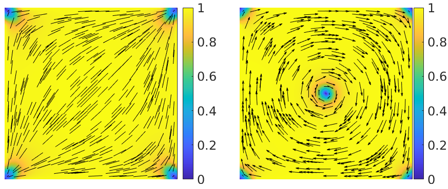
(a) $\mathbf{Q}_{D1}$ and $\mathbf{M}$ profile

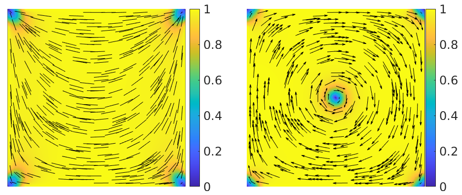
(b) $\mathbf{Q}_{R4}$ and $\mathbf{M}$ profile

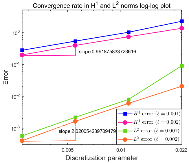
(c)

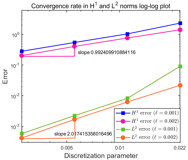
(d)

Figure 1: Nematic $\mathbf{Q}$ and magnetic $\mathbf{M}$ configurations: (a) D1 diagonal nematic and uncoupled magnetic profile and (b) R4 rotated nematic and uncoupled magnetic profile for the parameter values $\ell=0.001,c=0;$ Energy and $\mathbf{L}^{2}$ norm error versus discretization parameter $h$ plots for the discrete solutions (c) $\Psi_{h}=(\mathbf{Q}_{D1},\mathbf{M})$, (d) $\Psi_{h}=(\mathbf{Q}_{R4},\mathbf{M})$ for two sets of parameter values $\ell=0.001,c=0$ and $\ell=0.002,c=0$.

Case I: the coupling parameter $\mathbf{c=0}$

The two-dimensional planar bistable nematic device [26] (uncoupled system i.e., $c=0$) exhibits two sets of equilibrium configurations- 1) diagonally stable: the nematic directors roughly align along one of the square diagonals and there are two classes of diagonal solutions: D1 and D2, one for each square diagonal; 2) rotated states: here, the nematic director rotates by $\pi$ radians between a pair of opposite parallel edges, and there are $4$ classes of rotated solutions labelled by R1, R2, R3 and R4 respectively, related to each other by $\frac{\pi}{2}$ radians. The diagonal and rotated solutions are distinguished by the locations of the splay vertices; a splay vertex being a vertex such that the nematic director splays around the vertex and a bend vertex being such that the nematic director bends around the vertex in question. Each diagonal solution has a pair of diagonally opposite splay vertices and each rotated solution has a pair of adjacent splay vertices, connected by a square edge. In Figure 1(a) and Figure 1(b), the discrete solutions, $\Psi_{h}=(\mathbf{Q}_{D1},\mathbf{M})$ and $\Psi_{h}=(\mathbf{Q}_{R4},\mathbf{M})$, are plotted for $\ell=0.001,c=0$. Here $\mathbf{Q}_{D1}$ (resp. $\mathbf{Q}_{R4}$) is the D1 diagonal (resp. R4 rotated) solution with defects at vertices, and the corresponding nematic director $\mathbf{n}=(\cos\theta,\sin\theta)$ where $\theta=\frac{1}{2}\textrm{atan}\frac{Q_{D1,12}}{Q_{D1,11}}$ and $Q_{D1,11}=\frac{|\mathbf{Q}_{D1}|}{\sqrt{2}}\cos 2\theta,Q_{D1,12}=\frac{|\mathbf{Q}_{D1}|}{\sqrt{2}}\sin 2\theta$ are the two independent components of $\mathbf{Q}_{D1}$. Analogous remarks apply to $\mathbf{Q}_{R4}$. $\mathbf{M}$ labels the uncoupled magnetic profile with a $+1$-degree vortex at the square center consistent with topologically non-trivial boundary conditions. The magnetization vector $\mathbf{M}$ has a direction whereas the nematic director field, $\mathbf{n}$, is plotted without a direction since $\mathbf{n}$ and $-\mathbf{n}$ are physically equivalent. Figure 1(c) (resp. Figure 1(d)) demonstrate the convergence history of the discrete solutions, computed using piecewise polynomials of degree $1$, associated with D1 ( resp. R4) nematic solutions, in energy and $\mathbf{L}^{2}$ norms for the parameter values $\ell=0.001,c=0$ and $\ell=0.002,c=0$. The order $1$ convergence in energy norm and order $2$ convergence in $\mathbf{L}^{2}$- norm are obtained for both sets of parameter values. The color bars for nematic and magnetic profiles plot the values of $s=\sqrt{Q_{11}^{2}+Q_{12}^{2}}$ and $\left\lvert\mathbf{M}\right\rvert=\sqrt{M_{1}^{2}+M_{2}^{2}},$ respectively. The lines and arrows depict $\mathbf{n}$ and $\mathbf{M}$ respectively. Note that all subsequent discrete solution profiles, $\Psi_{h}$, have the nematic director field plot on the left and and magnetization vector plot on the right.

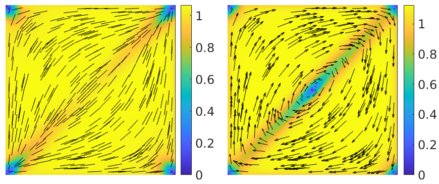
(a) $\mathbf{Q}_{D1}$ and $\mathbf{M}_{D1}$ profile

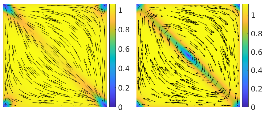
(b) $\mathbf{Q}_{D2}$ and $\mathbf{M}_{D2}$ profile

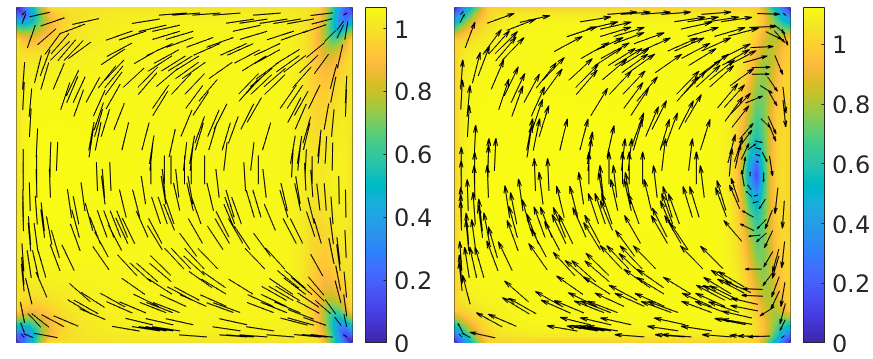
(c) $\mathbf{Q}_{R1}$ and $\mathbf{M}_{R1}$ profile

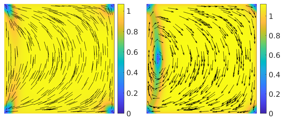
(d) $\mathbf{Q}_{R2}$ and $\mathbf{M}_{R2}$ profile

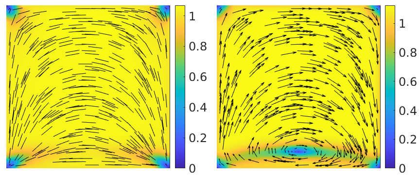
(e) $\mathbf{Q}_{R3}$ and $\mathbf{M}_{R3}$ profile

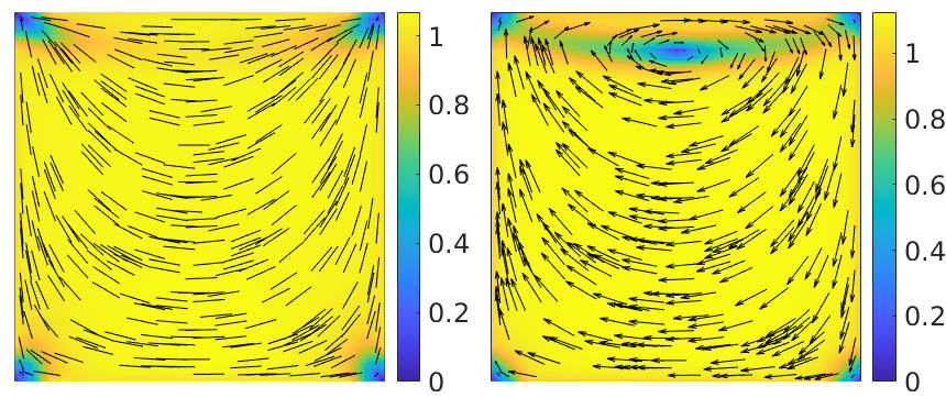
(f) $\mathbf{Q}_{R4}$ and $\mathbf{M}_{R4}$ profile

Figure 2: Nematic $\mathbf{Q}$ and magnetic $\mathbf{M}$ configurations for $\ell=0.001$ and $c=0.25.$ Left column: solution profiles $\Psi_{h}=(\mathbf{Q}_{D1},\mathbf{M}_{D1})$ (top) and $\Psi_{h}=(\mathbf{Q}_{D2},\mathbf{M}_{D2})$ (bottom) corresponding to diagonal D1 and D2 nematic stable solutions, respectively; Middle column: solution profiles $\Psi_{h}=(\mathbf{Q}_{R1},\mathbf{M}_{R1})$ (top) and $\Psi_{h}=(\mathbf{Q}_{R2},\mathbf{M}_{R2})$ (bottom) corresponding to rotated R1 and R2 nematic stable solutions, respectively; Right column: solution profiles $\Psi_{h}=(\mathbf{Q}_{R3},\mathbf{M}_{R3})$ (top) and $\Psi_{h}=(\mathbf{Q}_{R4},\mathbf{M}_{R4})$ (bottom) corresponding to rotated R3 and R4 nematic stable solutions, respectively.

Case II: the coupling parameter $\mathbf{c>0}$

Figure 2 plots the numerically computed stable solution profiles for parameter values $\ell=0.001,c=0.25$, represented by $\Psi_{h}=(\mathbf{Q}_{D1},\mathbf{M}_{D1}),$ $\Psi_{h}=(\mathbf{Q}_{D2},\mathbf{M}_{D2}),$ $\Psi_{h}=(\mathbf{Q}_{R1},\mathbf{M}_{R1}),$ $\Psi_{h}=(\mathbf{Q}_{R2},\mathbf{M}_{R2}),$ $\Psi_{h}=(\mathbf{Q}_{R3},\mathbf{M}_{R3}),$ $\Psi_{h}=(\mathbf{Q}_{R4},\mathbf{M}_{R4}),$ corresponding to D1, D2 diagonal and the R1, R2, R3, R4 rotated stable nematic equillibria, respectively. For small $\ell$, and $c>0,$ the coupling energy favors the co-alignment of $\mathbf{n}$ and $\mathbf{M}$, i.e., $\mathbf{n}\cdot\mathbf{M}=\pm 1.$ In this case, the nematic profiles (both diagonal and rotated) do not exhibit any interior vortices whereas the magnetic profiles develop an interior line of reduced $|\mathbf{M}|$, analogous to a domain wall, smeared out along the square diagonals/ near one of the square edges. The magnetic profiles, $\mathbf{M}_{D1},\mathbf{M}_{D2}$ (resp. $\mathbf{M}_{R1},\mathbf{M}_{R2}$, $\mathbf{M}_{R3},\mathbf{M}_{R4}$) exhibit $\pi$-walls [20] along the square diagonals $y=x$ for D1 and along $y=-x+1$ for D2 (resp. along the square edges $x=1$ for R1, $x=0$ for R2, $y=0$ for R3, $y=1$ for R4) nematic solutions. The domain walls are created to ensure the compatibility between the angle constraint in (2.2), the condition necessary to be minimizer for $c>0$, and the tangent boundary conditions. Recall that for $\mathbf{n}=(\cos\theta,\sin\theta)$, $Q_{11}=s\cos 2\theta$ and $Q_{12}=s\sin 2\theta.$ For a stable stationary point $\Psi=(s\cos 2\theta,s\sin 2\theta,\left\lvert\mathbf{M}\right\rvert\cos\varphi,\left\lvert\mathbf{M}\right\rvert\sin\varphi)$ with magnetization angle $\varphi$, (2.2) implies that

$$\theta\approx\varphi+k\pi,\,k\in\mathbb{Z}$$

almost everywhere in the domain interior , for sufficiently small values of $\ell$.

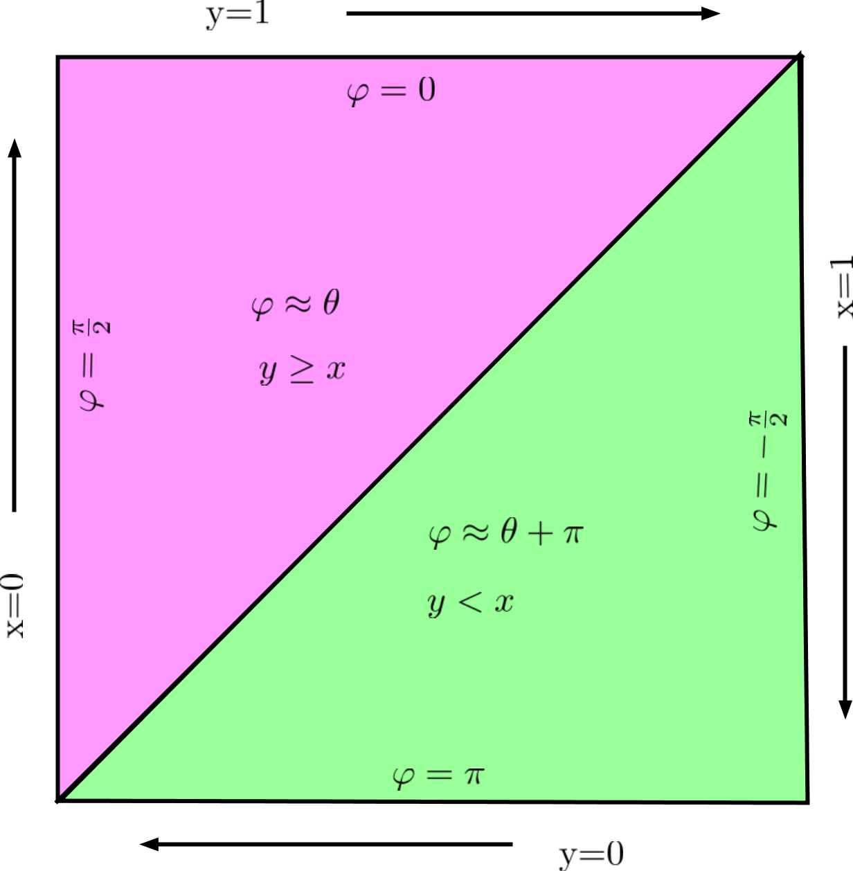
(a)

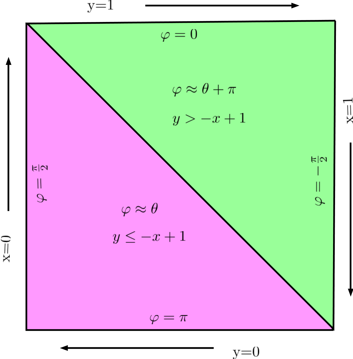
(b)

Figure 3: Domain wall formation of magnetic profiles (a) $\mathbf{M}_{D1}$ and (b) $\mathbf{M}_{D2}$.

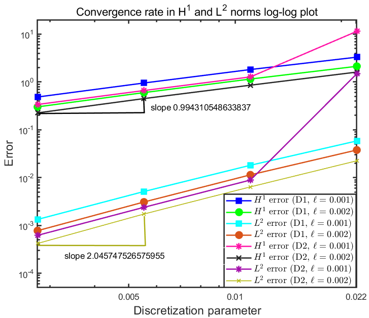
(a)

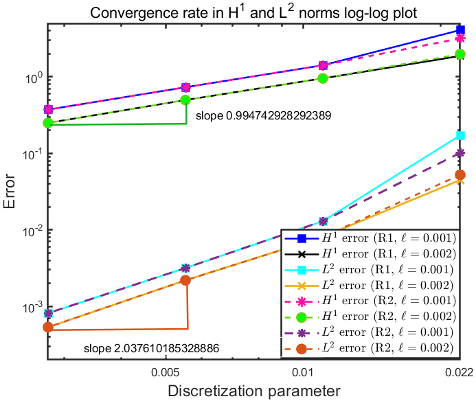
(b)

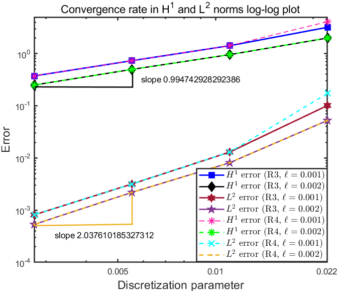
(c)

Figure 4: Energy and $\mathbf{L}^{2}$ norm error versus discretization parameter $h$ plots for the discrete solutions (a) $\Psi_{h}=(\mathbf{Q}_{D1},\mathbf{M}_{D1})$ and $\Psi_{h}=(\mathbf{Q}_{D2},\mathbf{M}_{D2})$, (b) $\Psi_{h}=(\mathbf{Q}_{R1},\mathbf{M}_{R1})$ and $\Psi_{h}=(\mathbf{Q}_{R2},\mathbf{M}_{R2})$, (c) $\Psi_{h}=(\mathbf{Q}_{R3},\mathbf{M}_{R3})$ and $\Psi_{h}=(\mathbf{Q}_{R4},\mathbf{M}_{R4}),$ for the two sets of parameter values $\ell=0.001,c=0.25,$ and $\ell=0.002,c=0.25,$

The tangent boundary condition for D1 ( resp. D2) nematic profile is coded in the boundary conditions: $\theta=0$ along $y=0,$ $\theta=0$ along $y=1,$ $\theta=\frac{\pi}{2}$ along $x=0,$ $\theta=\frac{\pi}{2}$ along $x=1$ (resp. $\theta=\pi$ along $y=0,$ $\theta=\pi$ along $y=1,$ $\theta=\frac{\pi}{2}$ along $x=0,$ $\theta=\frac{\pi}{2}$ along $x=1$). Figure (3) shows that $\theta\approx\varphi$ for $y\geq x$ (resp. $y\leq-x+1$) and $\theta\approx\varphi+\pi$ for $y<x$ (resp. $y>-x+1$) in $\mathbf{M}_{D1}$ (resp. $\mathbf{M}_{D2}$) profile. The domain walls for $\mathbf{M}_{R1},\mathbf{M}_{R2}$, $\mathbf{M}_{R3},\mathbf{M}_{R4}$ can be interpreted similarly. Figure 4 illustrates the numerical errors and orders of convergence, computed using piecewise polynomials of degree $1$, for the discrete solutions (a) $\Psi_{h}=(\mathbf{Q}_{D1},\mathbf{M}_{D1})$ and $\Psi_{h}=(\mathbf{Q}_{D2},\mathbf{M}_{D2})$, (b) $\Psi_{h}=(\mathbf{Q}_{R1},\mathbf{M}_{R1})$ and $\Psi_{h}=(\mathbf{Q}_{R2},\mathbf{M}_{R2})$, (c) $\Psi_{h}=(\mathbf{Q}_{R3},\mathbf{M}_{R3})$ and $\Psi_{h}=(\mathbf{Q}_{R4},\mathbf{M}_{R4})$, respectively, in energy and $\mathbf{L}^{2}$ norms for the parameter values $\ell=0.001,c=0.25$ and $\ell=0.002,c=0.25$. The convergence rates obtained in energy and $\mathbf{L}^{2}$ norms are of $\mathcal{O}(h)$ and $\mathcal{O}(h^{2})$, respectively.

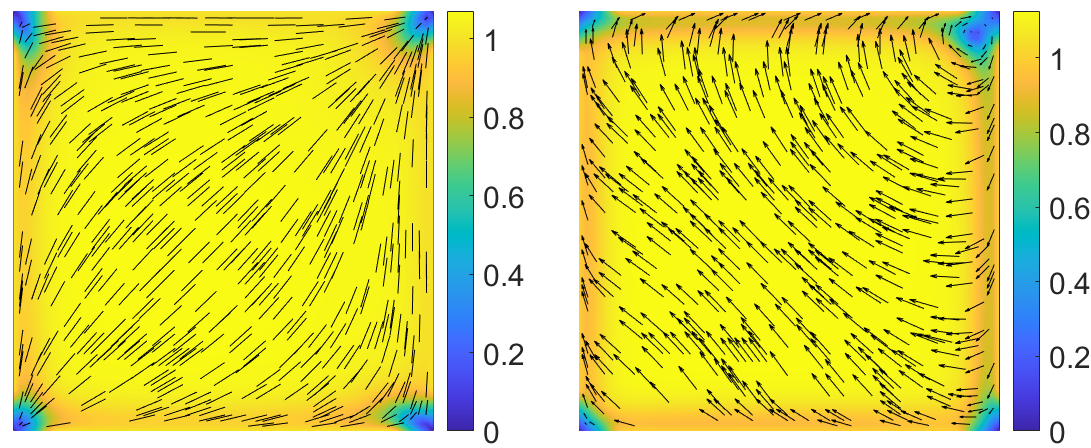
(a) $\mathbf{Q}_{D1}^{1}$ and $\mathbf{M}^{1}_{D1}$ profile

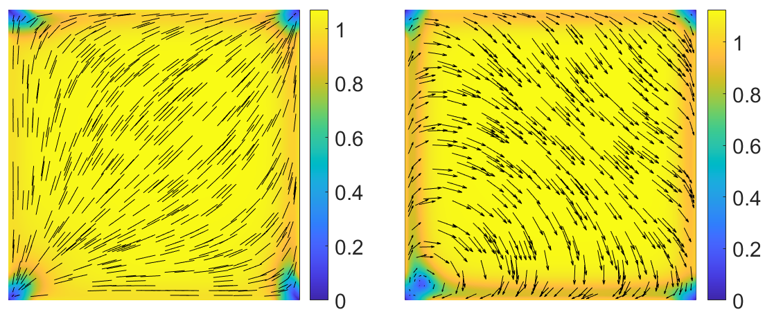
(b) $\mathbf{Q}_{D1}^{2}$ and $\mathbf{M}^{2}_{D1}$ profile

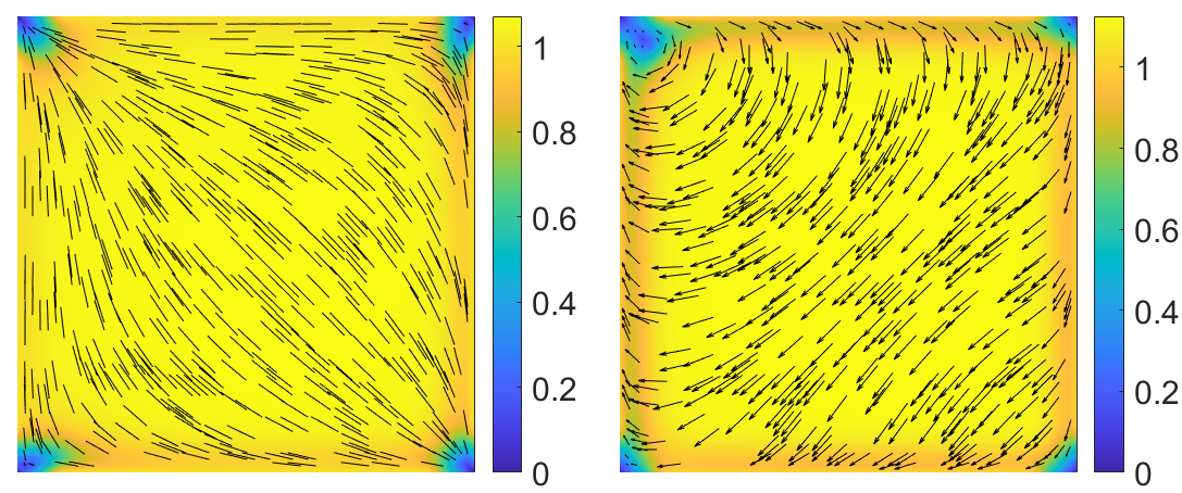
(c) $\mathbf{Q}^{1}_{D2}$ and $\mathbf{M}^{1}_{D2}$ profile

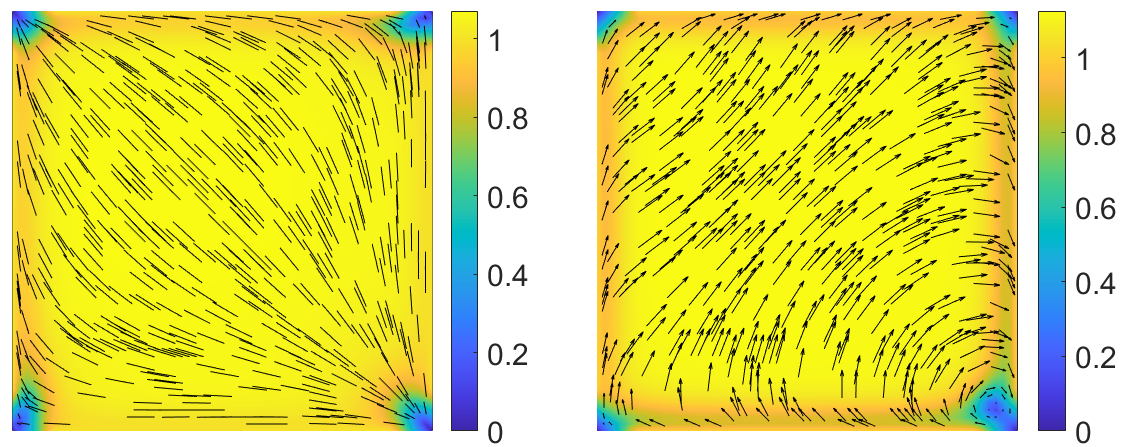
(d) $\mathbf{Q}^{2}_{D2}$ and $\mathbf{M}^{2}_{D2}$ profile

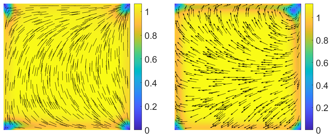
(e) $\mathbf{Q}^{1}_{R1}$ and $\mathbf{M}^{1}_{R1}$ profile

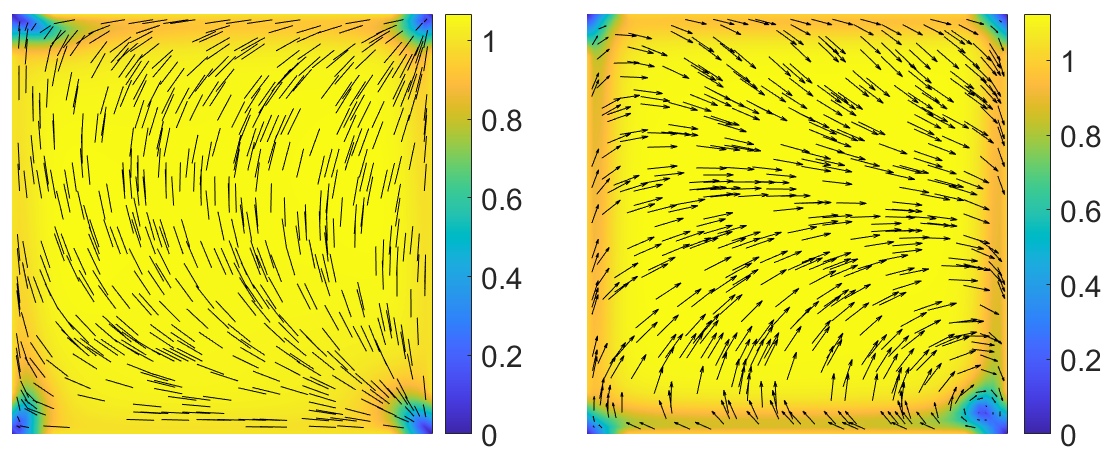
(f) $\mathbf{Q}^{2}_{R1}$ and $\mathbf{M}^{2}_{R1}$ profile

Figure 5: Nematic $\mathbf{Q}$ and magnetic $\mathbf{M}$ configurations for $\ell=0.001$ and $c=-0.25.$ Left column: two solution profiles $\Psi_{h}=(\mathbf{Q}^{1}_{D1},\mathbf{M}^{1}_{D1})$ and $\Psi_{h}=(\mathbf{Q}^{2}_{D1},\mathbf{M}^{2}_{D1})$ corresponding to diagonal D1 nematic stable solution; Middle column: two solution profiles $\Psi_{h}=(\mathbf{Q}^{1}_{D2},\mathbf{M}^{1}_{D2})$ and $\Psi_{h}=(\mathbf{Q}^{2}_{D2},\mathbf{M}^{2}_{D2})$ corresponding to diagonal D2 nematic stable solution; Right column: two solution profiles $\Psi_{h}=(\mathbf{Q}^{1}_{R1},\mathbf{M}^{1}_{R1})$ and $\Psi_{h}=(\mathbf{Q}^{2}_{R1},\mathbf{M}^{2}_{R2})$ corresponding to rotated R1 nematic stable solution.

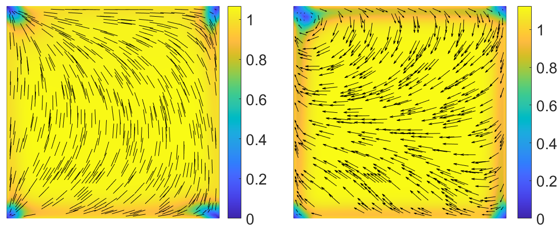
(a) $\mathbf{Q}^{1}_{R2}$ and $\mathbf{M}^{1}_{R2}$ profile

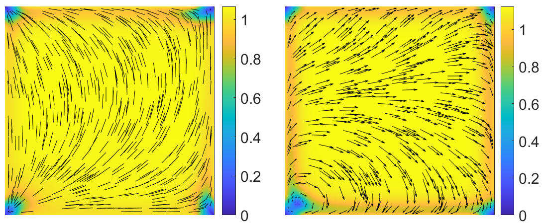
(b) $\mathbf{Q}^{2}_{R2}$ and $\mathbf{M}^{2}_{R2}$ profile

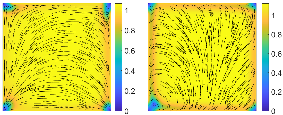
(c) $\mathbf{Q}^{1}_{R3}$ and $\mathbf{M}^{1}_{R3}$ profile

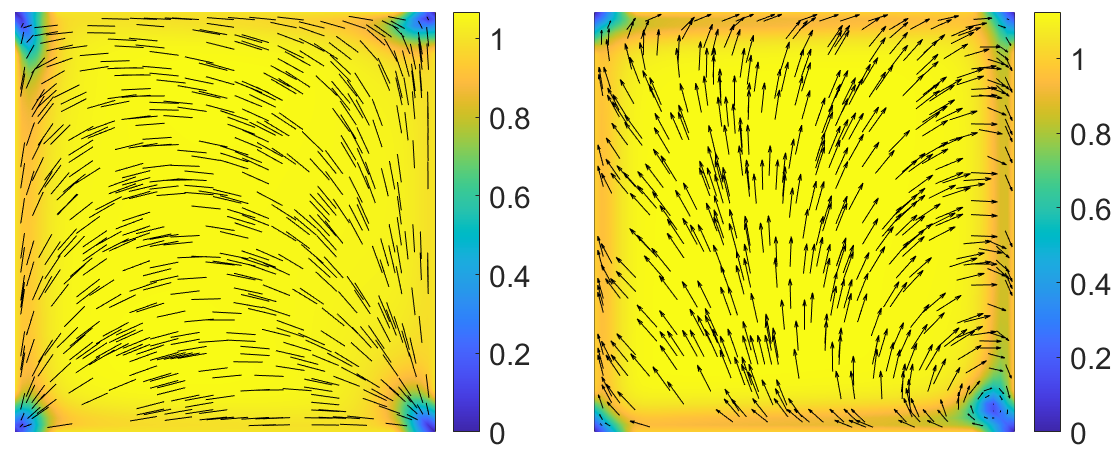
(d) $\mathbf{Q}^{2}_{R3}$ and $\mathbf{M}^{2}_{R3}$ profile

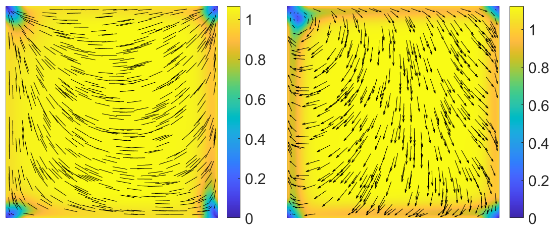
(e) $\mathbf{Q}^{1}_{R4}$ and $\mathbf{M}^{1}_{R4}$ profile

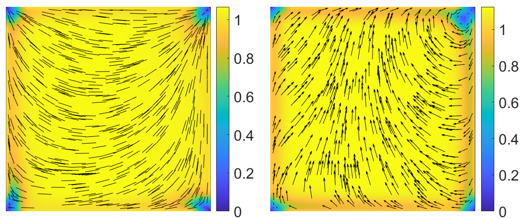
(f) $\mathbf{Q}^{2}_{R4}$ and $\mathbf{M}^{2}_{R4}$ profile

Figure 6: Nematic $\mathbf{Q}$ and magnetic $\mathbf{M}$ configurations for $\ell=0.001$ and $c=-0.25.$ Left column: two solution profiles $\Psi_{h}=(\mathbf{Q}^{1}_{R2},\mathbf{M}^{1}_{R2})$ and $\Psi_{h}=(\mathbf{Q}^{2}_{R2},\mathbf{M}^{2}_{R2})$ corresponding to rotated R2 nematic stable solution; Middle column: two solution profiles $\Psi_{h}=(Q^{1}_{R3},\mathbf{M}^{1}_{R3})$ and $\Psi_{h}=(\mathbf{Q}^{2}_{R3},\mathbf{M}^{2}_{R3})$ corresponding to rotated R3 nematic stable solution; Right column: two solution profiles $\Psi_{h}=(\mathbf{Q}^{1}_{R4},\mathbf{M}^{1}_{R4})$ and $\Psi_{h}=(\mathbf{Q}^{2}_{R4},\mathbf{M}^{2}_{R4})$ corresponding to rotated R4 nematic stable solution.

Case III: the coupling parameter $c<0$

Now, we discuss the discrete solution profiles for negative coupling, which favours perpendicular alignment of $\mathbf{n}$ and $\mathbf{M}$, i.e, $\mathbf{n}\cdot\mathbf{M}=0,$ for the parameter values $\ell=0.001$ and $c=-0.25.$ For diagonal nematic solutions (resp. rotated solutions), the symmetry between the diagonally opposite (resp. square edge) splay vertices is broken, so that there are $4$ distinct diagonal solutions. By similar reasoning, there are $8$ distinct rotated solutions, so that the number of stable admissible equilibria is doubled.

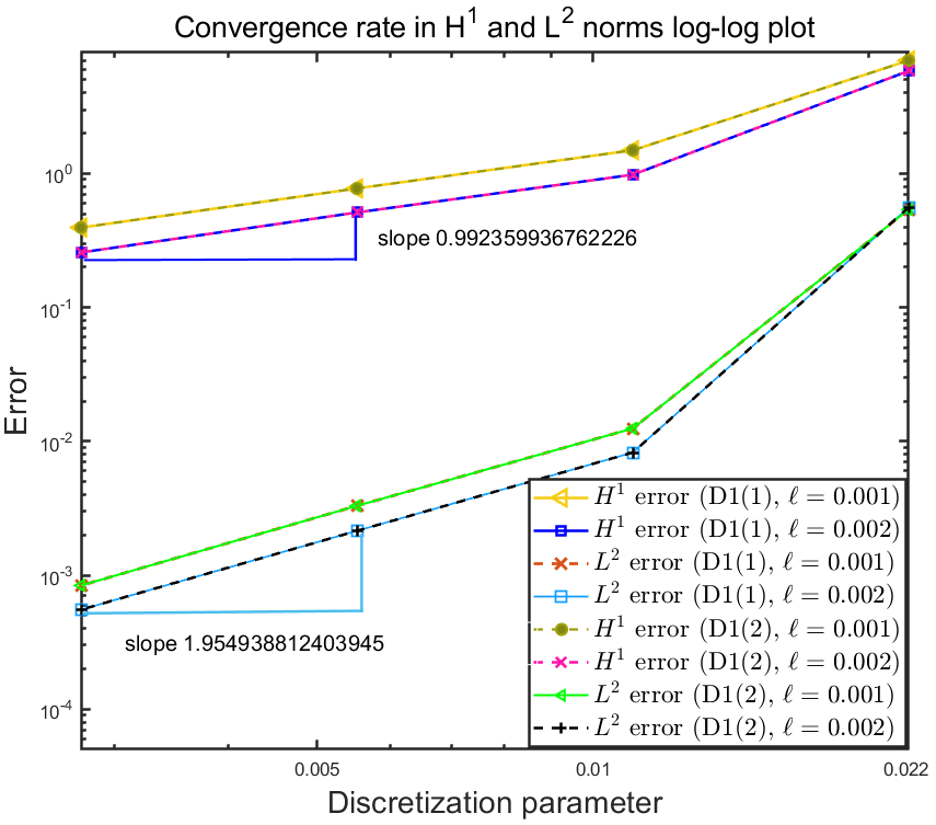
(a)

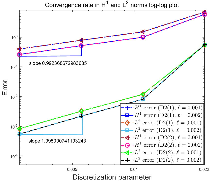
(b)

Figure 7: Energy and $\mathbf{L}^{2}$ norm errors versus discretization parameter $h$ plots for the discrete solutions (a) $\Psi_{h}=(\mathbf{Q}_{D1}^{1},\mathbf{M}_{D1}^{1})$ and $\Psi_{h}=(\mathbf{Q}_{D1}^{2},\mathbf{M}_{D1}^{2})$, (b) $\Psi_{h}=(\mathbf{Q}_{D2}^{1},\mathbf{M}_{D2}^{1})$ and $\Psi_{h}=(\mathbf{Q}_{D2}^{2},\mathbf{M}_{D2}^{2})$, for two sets of parameter values $\ell=0.001,c=-0.25,$ and $\ell=0.002,c=-0.25.$

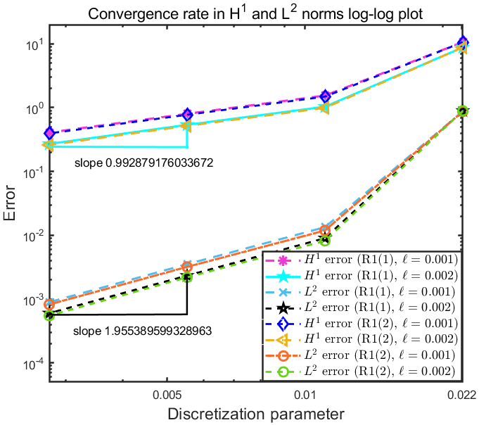
(a)

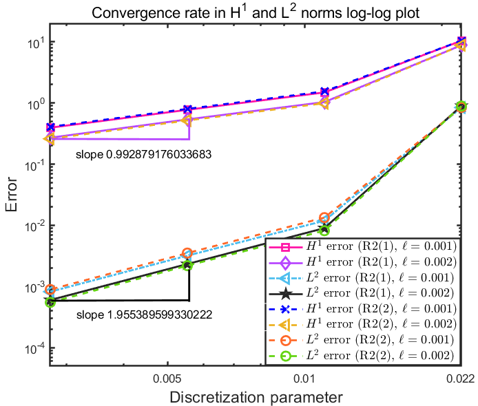
(b)

Figure 8: Energy and $\mathbf{L}^{2}$ norm errors versus discretization parameter $h$ plots for the discrete solutions (a) $\Psi_{h}=(\mathbf{Q}_{R1}^{1},\mathbf{M}_{R1}^{1})$ and $\Psi_{h}=(\mathbf{Q}_{R1}^{2},\mathbf{M}_{R1}^{2})$, (b) $\Psi_{h}=(\mathbf{Q}_{R2}^{1},\mathbf{M}_{R2}^{1})$ and $\Psi_{h}=(\mathbf{Q}_{R2}^{2},\mathbf{M}_{R2}^{2})$, for two sets of parameter values $\ell=0.001,c=-0.25,$ and $\ell=0.002,c=-0.25.$

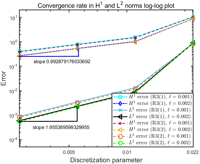
(a)

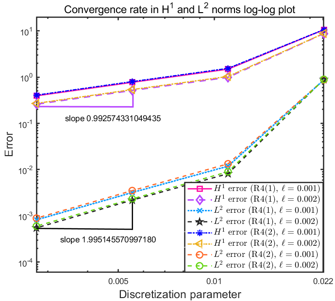
(b)

Figure 9: Energy and $\mathbf{L}^{2}$ norm errors versus discretization parameter $h$ plots for the discrete solutions, (a) $\Psi_{h}=(\mathbf{Q}_{R3}^{1},\mathbf{M}_{R3}^{1})$ and $\Psi_{h}=(\mathbf{Q}_{R3}^{2},\mathbf{M}_{R3}^{2})$, (b) $\Psi_{h}=(\mathbf{Q}_{R4}^{1},\mathbf{M}_{R4}^{1})$ and $\Psi_{h}=(\mathbf{Q}_{R4}^{2},\mathbf{M}_{R4}^{2}),$ for two sets of parameter values $\ell=0.001,c=-0.25,$ and $\ell=0.002,c=-0.25.$

For instance, $\Psi_{h}=(\mathbf{Q}_{D1}^{1},\mathbf{M}_{D1}^{1})$ and $\Psi_{h}=(\mathbf{Q}_{D1}^{2},\mathbf{M}_{D1}^{2})$ in Figure 5 are two distinct stable, numerically computed solutions corresponding to standard D1 diagonal nematic profile (for $c=0$). Similarly, there are ten pairs of distinct stable solution profiles, corresponding to the standard D2, R1, R2, R3 and R4 profiles; see Figures 5 and 6. The numerical errors and orders of convergence of the discrete solutions associated with the diagonal (D1, D2), and rotated (R1, R2) and (R3, R4) nematic equilibria are plotted in Figures 7, 8 and 9, respectively, for two sets of parameter values $\ell=0.001,c=-0.25$ and $\ell=0.002,c=-0.25$. The convergence rates in energy and $\mathbf{L}^{2}$ norms are noted to be of order, $O(h)$ and $O(h^{2})$, respectively.

Parameter dependent plots

Figure 10 (resp. Figure 11) presents discretization parameter $h$ versus energy and $\mathbf{L}^{2}$ norm error plots, for various values of $\ell$ and positive coupling (resp. negative coupling) parameter, for the discrete solution corresponding to D1 diagonal nematic equillibria. We observe that both the energy and $\mathbf{L}^{2}$ norm errors are sensitive to the choice of the small parameter $\ell$, for both instances of positive and negative nemato-magnetic coupling. For instance, fix $h=10^{-2},$ the energy norm error for $\ell=0.01$ at $h=10^{-2}$ is smaller than the error for $\ell=0.006$ and similarly, the error increases as $\ell$ further decreases.

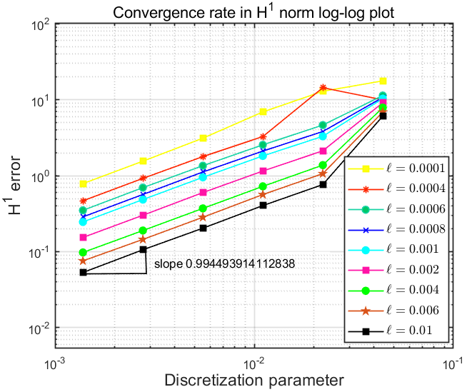
(a)

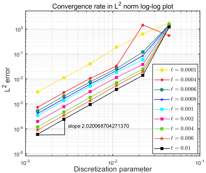
(b)

Figure 10: Convergence behavior plots of error in the (a) energy norm and (b) $\mathbf{L}^{2}$ norm versus the discretization parameter $h$ for $\Psi_{h}:=(\mathbf{Q}_{D1},\mathbf{M}_{D1})$ solution for various values of $\ell$ and $c=0.25.$

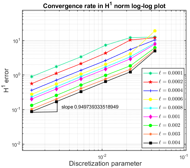
(a)

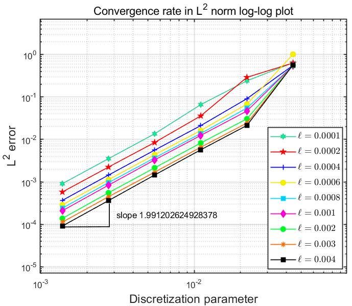
(b)

Figure 11: Convergence behavior plots of error in the (a) energy norm and (b) $\mathbf{L}^{2}$ norm versus the discretization parameter $h$ for $\Psi_{h}:=(\mathbf{Q}_{D1}^{1},\mathbf{M}_{D1}^{1})$ solution for various values of $\ell$ and $c=-0.25.$

Remark 4.1.

The Landau-de Gennes energy for nematic liquid crystal is defined [26] as

$$F_{\text{nem}}(\bar{{\Psi}}_{\epsilon})=\int_{\Omega}(\left\lvert\nabla\bar{{\Psi}}_{\epsilon}\right\rvert^{2}+\epsilon^{-2}(\left\lvert\bar{{\Psi}}_{\epsilon}\right\rvert^{2}-1)^{2})\,{\rm dx},$$

where $\bar{{\Psi}}_{\epsilon}:=(u_{1},u_{2})=\bar{g}$ on $\partial\Omega$ and $\epsilon$ is a material-dependent parameter that depends on the elastic constant, domain size and temperature. The Euler-Lagrange equations are a system of second order non-linear elliptic partial differential equations that seeks $\bar{{\Psi}}_{\epsilon}\in X\times X$ such that for all $\bar{\varphi}:=(\varphi_{1},\varphi_{2})\in V\times V$

$$\int_{\Omega}\nabla u_{1}\cdot\nabla\varphi_{1}\,{\rm dx}+2\epsilon^{-2}\int_{\Omega}(u_{1}^{2}+u_{2}^{2}-1)u_{1}\varphi_{1}\,{\rm dx}=0,$$

$$\int_{\Omega}\nabla u_{2}\cdot\nabla\varphi_{2}\,{\rm dx}+2\epsilon^{-2}\int_{\Omega}(u_{1}^{2}+u_{2}^{2}-1)u_{2}\varphi_{2}\,{\rm dx}=0,$$

which is (3.2) for ${\Psi}:=(u_{1},u_{2},0,0)$ and ${\Phi}:=(\varphi_{1},\varphi_{2},0,0)$ with the parameter values $\ell=\frac{\epsilon^{2}}{2}.$ Note that the non-linearity in reduced Landau-de Gennes minimization problem is cubic. The quadratic non-linear term $B_{2}(\cdot,\cdot,\cdot)$ in (3.2) is zero here. An a priori error analysis with $h-\epsilon$ dependency has been discussed for this model for discontinuous Galerkin method in [33]. The analysis for conforming finite element method is a special case of the problem considered in this paper. ∎

5 Conclusions

We study the minimizers of a $\mathbf{Q}$-tensor -$\mathbf{M}$ model for dilute ferronematic suspensions in 2-D framework. The energy functional has two parameters- a scaled elastic parameter $\ell$ and nemato-magnetic coupling parameter $c$. We analyze the asymptotic behavior of the global minimizers of $\tilde{\mathcal{E}}$, as $\ell\rightarrow 0$ and establish that ${|\kern-1.07639pt|\kern-1.07639pt|\Psi^{\ell}|\kern-1.07639pt|\kern-1.07639pt|}_{2}$ is bounded, independent of $\ell.$ This result plays a key role in the $h-\ell$ dependent finite element analysis for regular solutions of the corresponding Euler-Lagrange PDEs such that (3.1) holds. Whether the analysis holds for all regular solutions of the Euler-Lagrange PDEs is proposed as future work. The numerical results focus on the solution landscapes for $\ell=0.001,c=0,\pm 0.25$ in a square domain, the convergence rates in energy and $\mathbf{L}^{2}$ norms, the convergence behavior of discrete solutions for various values of $\ell$. The numerical results in this manuscript can be extended to stable solutions, for other values of $c$ and $\ell$ as reported in [3]. The convergence of minimizers in $\mathbf{L}^{\infty}$ norm i.e., ${|\kern-1.07639pt|\kern-1.07639pt|\Psi^{\ell}-\Psi_{0}|\kern-1.07639pt|\kern-1.07639pt|}_{\infty}$ estimates, the analysis for three-dimensional geometries, the finite element analysis for polygonal domains with re-entrant corners and Dirichlet boundary data with lesser regularity, a posteriori error analysis to investigate the effects of defects on numerical errors are interesting and challenging extensions of this work. Moreover, the asymptotic analysis of minimizers with topologically non-trivial boundary conditions and/or $\ell$-dependent Dirichlet boundary data $\mathbf{g}_{\ell}$, including star-shaped domains, are further interesting areas to be investigated.

References

[1]
F. Bethuel, H. Brezis, and F. Hélein, Asymptotics for the
minimization of a Ginzburg-Landau functional, Calculus of Variations and
Partial Differential Equations 1 (1993), no. 2, 123–148.
[2]
, Ginzburg-Landau vortices, Modern Birkhäuser Classics,
Birkhäuser/Springer, Cham, 2017, Reprint of the 1994 edition.
[3]
K. Bisht, Y. Wang, V. Banerjee, and A. Majumdar, Tailored morphologies in
two-dimensional ferronematic wells, Physical Review E 101 (2020),
022706.
[4]
J. P. Borthagaray, R. H. Nochetto, and S. W. Walker, A
structure-preserving FEM for the uniaxially constrained Q-tensor model of
nematic liquid crystals, Numerische Mathematik 145 (2020), no. 4,
837–881.
[5]
F. Brochard and P. G. de Gennes, Theory of magnetic suspensions in liquid
crystals, Journal De Physique 31 (1970), no. 7, 691–708.
[6]
S. V. Burylov and Y. L. Raikher, Macroscopic properties of ferronematics
caused by orientational interactions on the particle surfaces. I. extended
continuum model, Molecular Crystals and Liquid Crystals Science and
Technology. Section A. 258 (1995), no. 1, 107–122.
[7]
M. C. Calderer, A. DeSimone, D. Golovaty, and A. Panchenko, An effective
model for nematic liquid crystal composites with ferromagnetic inclusions,
SIAM Journal on Applied Mathematics 74 (2014), no. 2, 237–262.
[8]
P. G. Ciarlet, The finite element method for elliptic problems, Classics
in Applied Mathematics, vol. 40, Society for Industrial and Applied
Mathematics (SIAM), Philadelphia, PA, 2002.
[9]
C. Cîrtoaje, E. Petrescu, C. Stan, and D. Creangă, Ferromagnetic
nanoparticles suspensions in twisted nematic, Physica E: Low-dimensional
Systems and Nanostructures 79 (2016), 38 – 43.
[10]
J. Dalby, Farrell P. E., Majumdar A., and J. Xia, One-dimensional
ferronematics in a channel: order reconstruction, bifurcations and
multistability, https://arxiv.org/abs/2102.06347 (2021).
[11]
T. A. Davis and E. C. Gartland, Jr., Finite element analysis of the
Landau-de Gennes minimization problem for liquid crystals, SIAM Journal
on Numerical Analysis 35 (1998), no. 1, 336–362.
[12]
P. de Gennes and J. Prost, The physics of liquid crystals, International
Series of Monogr, Clarendon Press, 1993.
[13]
D. A. Di Pietro and A. Ern, Mathematical aspects of discontinuous
Galerkin methods, Mathématiques & Applications (Berlin) [Mathematics
& Applications], vol. 69, Springer, Heidelberg, 2012.
[14]
A. Ern and J-L. Guermond, Theory and practice of finite elements,
Applied Mathematical Sciences, vol. 159, Springer-Verlag, New York, 2004.
[15]
L. C. Evans, Partial differential equations, second ed., Graduate
Studies in Mathematics, vol. 19, American Mathematical Society, Providence,
RI, 2010.
[16]
C. Giacomo, Biaxiality in the asymptotic analysis of a 2D Landau–de
Gennes model for liquid crystals, ESAIM. Control, Optimisation and
Calculus of Variations 21 (2015), no. 1, 101–137.
[17]
D. Golovaty, J. Alberto Montero, and P. Sternberg, Dimension reduction
for the Landau-de Gennes model in planar nematic thin films, Journal of
Nonlinear Science 25 (2015), 1431 – 1451.
[18]
P. Grisvard, Elliptic problems in nonsmooth domains, Classics in Applied
Mathematics, vol. 69, Society for Industrial and Applied Mathematics (SIAM),
Philadelphia, PA, 2011.
[19]
M. D. Gunzburger and S. L. Hou, Treating inhomogeneous essential boundary
conditions in finite element methods and the calculation of boundary
stresses, SIAM Journal on Numerical Analysis 29 (1992), no. 2,
390–424.
[20]
Y. Han, J. Harris, Majumdar A., and J. Walton, Tailored morphologies in
two-dimensional ferronematic wells, Physical Review E (2021).
[21]
Y. Han, A. Majumdar, and L. Zhang, A reduced study for nematic equilibria
on two-dimensional polygons, SIAM Journal on Applied Mathematics 80
(2020), no. 4, 1678–1703.
[22]
H. B. Keller, Approximation methods for nonlinear problems with
application to two-point boundary value problems, Mathematics of Computation
29 (1975), 464–474.
[23]
S. Kesavan, Topics in functional analysis and applications, John Wiley
& Sons, Inc., New York, 1989.
[24]
J. P.F. Lagerwall and G. Scalia, A new era for liquid crystal research:
Applications of liquid crystals in soft matter nano-, bio- and
microtechnology, Current Applied Physics 12 (2012), no. 6,
1387–1412.
[25]
J.-L. Lions and E. Magenes, Non-homogeneous boundary value problems and
applications. Vol. I, Springer-Verlag, New York-Heidelberg, 1972,
Translated from the French by P. Kenneth, Die Grundlehren der mathematischen
Wissenschaften, Band 181.
[26]
C. Luo, A. Majumdar, and R. Erban, Multistability in planar liquid
crystal wells, Physical Review E 85 (2012), 061702.
[27]
R. R. Maity, A. Majumdar, and N. Nataraj, Error analysis of Nitsche’s
and discontinuous Galerkin methods of a reduced Landau–de Gennes
problem, Computational Methods in Applied Mathematics 21 (2021),
no. 1, 179 – 209.
[28]
A. Majumdar and A. Zarnescu, Landau-de Gennes theory of nematic liquid
crystals: the Oseen-Frank limit and beyond, Archive for Rational
Mechanics and Analysis 196 (2010), no. 1, 227–280.
[29]
A. Mertelj and D. Lisjak, Ferromagnetic nematic liquid crystals, Liquid
Crystals Reviews 5 (2017), no. 1, 1–33.
[30]
A. Mertelj, D. Lisjak, M. Drofenik, and M. Copič, Ferromagnetism in
suspensions of magnetic platelets in liquid crystal, Nature 504
(2013), no. 7479, 237—241.
[31]
R. Moser, Partial regularity for harmonic maps and related problems,
World Scientific Publishing Co. Pte. Ltd., Hackensack, NJ, 2005.
[32]
J. Nitsche, Über ein variationsprinzip zur lösung von
dirichlet-problemen bei verwendung von teilräumen, die keinen
randbedingungen unterworfen sind, Abhandlungen aus dem Mathematischen
Seminar der Universität Hamburg 36 (1971), no. 1, 9–15.
[33]
R. R. Maity, A. Majumdar, and N. Nataraj, Discontinuous Galerkin finite
element methods for the Landau–de Gennes minimization problem of liquid
crystals, IMA Journal of Numerical Analysis 41 (2021), no. 2,
1130–1163.
[34]
M. Slavinec, E. Klemenčič, M. Ambrožič, and M. Krasna, Impact of
nanoparticles on nematic ordering in square wells, Advances in Condensed
Matter Physics 2015 (2015), 1–11.
[35]
C. Tsakonas, A. J. Davidson, C. V. Brown, and N. J. Mottram, Multistable
alignment states in nematic liquid crystal filled wells, Applied Physics
Letters 90 (2007), Article 111913.
[36]
W. Wang, L. Zhang, and P. Zhang, Modeling and computation of liquid
crystals, Acta Numerica (2022).
[37]
Y. Wang, G. Canevari, and A. Majumdar, Order reconstruction for nematics
on squares with isotropic inclusions: a Landau–de Gennes study, SIAM
Journal on Applied Mathematics 79 (2019), no. 4, 1314–1340.