Parameter symmetries of neutrino oscillations in vacuum, matter,
and approximation schemes

Abstract

Expressions for neutrino oscillations contain a high degree of symmetry, but typical forms for the oscillation probabilities mask these symmetries of the oscillation parameters. We elucidate the $2^{7}$ parameter symmetries of the vacuum parameters and draw connections to the choice of definitions of the parameters as well as interesting degeneracies. We also show that in the presence of matter an additional set of $2^{7}$ parameter symmetries exist of the matter parameters. Due to the complexity of the exact expressions for neutrino oscillations in matter, numerous approximations have been developed; we show that under certain assumptions, approximate expressions have at most $2^{6}$ additional parameter symmetries of the matter parameters. We also include one parameter symmetry related to the LMA-Dark degeneracy that holds under the assumption of CPT invariance; this adds one additional factor of two to all of the above cases. Explicit, non-trivial examples are given of how physical observables in neutrino oscillations, such as the probabilities, CP violation, the position of the solar and atmospheric resonance, and the effective $\Delta m^{2}$’s for disappearance probabilities, are invariant under all of the above symmetries. We investigate which of these parameter symmetries apply to numerous approximate expressions in the literature and show that a more careful consideration of symmetries improves the precision of approximations.

I Introduction

The propagation of neutrinos is described by the eigenvalues and eigenvectors of the Hamiltonian. The eigenvectors form up into a unitary matrix which, after rephasing of the charged leptons and the neutrinos results in four degrees of freedom. There are a considerable number of options for parameterizing the matrix, see e.g. Denton and Pestes (2021) for a recent overview. Even within one parameterization scheme, there may still be a large number of choices to be made, and that is the focus of this paper.

The lepton mixing matrix Pontecorvo (1957); Maki et al. (1962) is usually described Zyla et al. (2020) as the product of three rotations: (23), (13), (12), with a complex phase associated with the (13) rotation resulting in four different physical degrees of freedom: $\theta_{23}$, $\theta_{13}$, $\theta_{12}$, and $\delta$. Distilling the 18 degrees of freedom of a complex $3\times 3$ matrix down to four parameters is due to the fact that the mixing matrix is unitary, but any choice of parameterization as a sequence of rotations leaves a number of discrete symmetries of the parameters including the usual PDG choice. Once the order of rotations is chosen and the parametrization is made, there are still many different configurations that result in the same physics. The parameter symmetries that connect these different configurations are directly related to the definition of the range of the parameters , see e.g. Gluza and Zralek (2001). Typically the initial definition made is to restrict the ranges of the three mixing angles from $[0,2\pi)$ down to $[0,\pi/2)$ - a factor of four reduction for each angle. That implies that each quadrant of each angle can be related to the other quadrants, implying $4^{3}=64$ discrete parameter symmetries. This means that for any given configuration of the mixing angles, there are 63 others that lead to exactly equivalent physics. There is also one discrete parameter symmetry which again doubles the number of parameter symmetries related to the choice of how one defines the mass eigenstates Denton (2020). This leads to a total of $2^{7}=128$ discrete parameter symmetries. Ref. Gluza and Zralek (2001) concentrated on the allowed range for each parameter, where in this paper we concentrate on the non-trivial parameter symmetries of the physical oscillation observables when written in terms of mixing angles and a phase. These parameter symmetries restrict the allowed combinations of such parameters which we elucidate with important examples. In addition, ref. Gonzalez-Garcia et al. (2011) assumed CP conservation and vanishing $\Delta m^{2}_{21}$ and examined a subset of the symmetries presented in this work to determine the allowed ranges of the parameters. In addition, if one generalizes the mixing matrix to include a phase on each rotation, there are two additional continuous degrees of freedom related to rephasing of the neutrino states or the Majorana phases. In this paper we show exactly how all of the parameter symmetries arise.

Going beyond the symmetries of the vacuum parameters which can all be addressed via a choice of definition of the mixing angles and mass eigenstates, these parameter symmetries also naturally extend to the mixing angles and eigenvalues in matter as well, providing another $2^{7}=128$ discrete parameter symmetries. Since both of these sets of symmetries apply simultaneously in matter, there are in total $2^{14}=16,384$ discrete parameter symmetries of the oscillation probabilities in matter for both neutrinos and anti-neutrinos.

The above symmetries all leave the Hamiltonian unchanged up to rephasing. There is an additional parameter symmetry which changes the Hamiltonian but leaves all physical observables unchanged known as the CPT parameter symmetry. This is due to the fact that, under the assumption that CPT is a good symmetry, all of the oscillation physics is unchanged by the transformation $H\to-H^{*}$. This symmetry, when combined with some of the others discussed above, is equivalent to the so-called LMA-Light – LMA-Dark symmetry often discussed in the literature de Gouvea et al. (2000); Miranda et al. (2006); Bakhti and Farzan (2014); Coloma and Schwetz (2016); Denton et al. (2018a). This leads to an additional power of two for the total number of symmetries for each of the vacuum case, the matter case, and approximate case.

It is well known that the exact solutions to neutrino oscillations in constant matter density are quite intractable. To gain insights on the physics of neutrino oscillations in matter, a large number of approximate expressions have been developed. We also examine these parameter symmetries in the scenario of a perturbative Hamiltonian. The symmetries of both the vacuum parameters and the new approximate parameters also apply subject to certain conditions, one of which restricts the number of parameter symmetries of the perturbative parameters by two to bring the total number of parameter symmetries for a perturbative scheme to $2^{13}=8,192$. Finally, we examine which of these parameter symmetries are satisfied by various approximate expressions in the literature.

II Parameter symmetries

Since the Hamiltonian in the flavor basis uniquely and exactly determines the neutrino oscillation probabilities, any parameter symmetry of this Hamiltonian is necessarily a parameter symmetry of the probabilities. We first focus on the vacuum case for simplicity, and will later show that the presence of matter, handled either exactly or perturbatively, behaves in a similar way. We define the Hamiltonian in the usual PDG fashion Zyla et al. (2020) except with a complex phase on each rotation,

$$H_{\rm flav}=\frac{1}{2E}U_{23}U_{13}U_{12}M^{2}U_{12}^{\dagger}U_{13}^{\dagger}U_{23}^{\dagger}\,,$$ (1)

where the nontrivial part of the $2\times 2$ submatrix of the $3\times 3$ complex rotation matrices are defined as

$$U_{ij}(\theta_{ij},\delta_{ij})=\begin{pmatrix}c_{ij}&s_{ij}e^{i\delta_{ij}}\\ -s_{ij}e^{-i\delta_{ij}}&c_{ij}\end{pmatrix}\,,$$ (2)

and the mass-squared matrix is $M^{2}=\operatorname{diag}(m_{1}^{2},m_{2}^{2},m_{3}^{2})$. That is, we describe the mixing matrix with three rotation angles $\theta_{ij}$ and three associated complex phases $\delta_{ij}$. To understand the parameter symmetries it is useful to work with this slightly more general mixing matrix with three distinct complex phases, one for each rotation, however ultimately oscillation probabilities only depend on the sum of these three complex phases.

II.1 Discrete parameter symmetries

We now list the various parameter symmetries of the Hamiltonian. First, there are 128 discrete parameter symmetries of the vacuum Hamiltonian up to rephasing. To describe these we introduce the parameters $m_{ij}$ and $n_{ij}$ each of which are $\in\mathbb{Z}_{2}$ (that is, $\{0,1\}$). A sign flip of a cosine term is given by the $m_{ij}$ parameters: $c_{ij}\to(-1)^{m_{ij}}c_{ij}$ and a sign flip of a sine term is given by the $n_{ij}$ parameters: $s_{ij}\to(-1)^{n_{ij}}s_{ij}$. This allows us to write down “angle reflection” ($n_{ij}$) and “angle shift and reflection” ($m_{ij}$) parameter symmetries as follows:

• $(i,j)=(2,3)$ or $(1,2)$:

  $$c_{ij}\to(-1)^{m_{ij}}c_{ij}\,,\ s_{ij}\to(-1)^{n_{ij}}s_{ij}$$

  $$\text{ so long as }\delta_{ij}\to\delta_{ij}+(m_{ij}+n_{ij})\pi\,.$$ (3)

• $(i,j)=(1,3)$:

  $$c_{13}\to(-1)^{m_{13}}c_{13}\,,\ s_{13}\to(-1)^{n_{13}}s_{13}$$

  $$\text{ so long as }\delta_{13}\to\delta_{13}+n_{13}\pi\,.$$ (4)

In each case, if one of the angles is changed via the $m_{ij}$ or $n_{ij}$ parameters then the corresponding $\delta_{ij}$ must accumulate a factor of $\pi$ with the exception of changes to $c_{13}$. That is, the six $m_{ij}$ and $n_{ij}$ are all independent and can each be either zero or one, leading to $2^{6}=64$ combinations.

The remaining discrete parameter symmetry is the 1-2 interchange Denton et al. (2016) for which all of the following simultaneously happen,

• $(i,j)=(1,2)$:

  $$c_{12}\to s_{12}\text{ and }s_{12}\to c_{12}$$

  $$\text{ so long as }\delta_{12}\to\delta_{12}+\pi\text{ and }m_{1}^{2}\leftrightarrow m_{2}^{2}\,.$$ (5)

The final part of the interchange is equivalent to $\Delta m^{2}_{21}\to\Delta m^{2}_{12}=-\Delta m^{2}_{21}$ and $\Delta m^{2}_{31}\leftrightarrow\Delta m^{2}_{32}$. Note that the 1-2 interchange can be done simultaneously with the shift and reflection described above. The parameter symmetry related to this interchange provides one more factor of two leading to 128 total parameter symmetries.

After performing any combination of these parameter symmetries including the 1-2 interchange, the Hamiltonian is exactly the same up to a possible overall phase matrix,

$$H_{\rm flav}\to$$ (6)

$$\operatorname{diag}((-1)^{m_{13}+m_{23}},1,1)H_{\rm flav}\operatorname{diag}((-1)^{m_{13}+m_{23}},1,1)\,,$$

see appendix A for an explicit derivation of this. This $(-1)$ phase coming from $m_{13}$ and/or $m_{23}$ terms can then be absorbed into the definition of $|\nu_{e}\rangle$ and nothing has changed. The presence of $m_{13}$ and $m_{23}$ and not $m_{12}$ is due to the fact that the sign from sending $c_{12}\to-c_{12}$ can go through the middle of the Hamiltonian and commutes with the $M^{2}$ matrix, while this isn’t true for the $m_{13}$ or $m_{23}$ parameter symmetries. The $n_{ij}$ parameter symmetries operate on the rotation matrix level and thus do not affect the total Hamiltonian.

The various interchanges can be thought of equally in terms of sines and cosines (e.g. $s\to-s$) or in terms of angles (e.g. $\theta\to-\theta$). For convenience we include the relationship between these in a table:

sines/cosines	angles
$s\to-s$, $c\to c$	$\theta\to-\theta$
$s\to s$, $c\to-c$	$\theta\to\pi-\theta$
$s\to-s$, $c\to-c$	$\theta\to\pi+\theta$
$c\to s$, $s\to c$	$\theta\to\pi/2-\theta$
$c\to-s$, $s\to c$	$\theta\to\pi/2+\theta$
$c\to s$, $s\to-c$	$\theta\to-\pi/2+\theta$
$c\to-s$, $s\to-c$	$\theta\to-\pi/2-\theta$

II.2 Continuous parameter symmetries

In addition to the above discrete parameter symmetries, there are two continuous degrees of freedom as well dubbed the “delta shuffle”. We define the three rotations and complex phases by

$$U_{23}(\theta_{23},\delta_{23})U_{13}(\theta_{13},-\delta_{13})U_{12}(\theta_{12},\delta_{12})\,.$$ (7)

In fact, in the context of neutrino oscillations, these three phases are related by

$$\delta_{23}+\delta_{13}+\delta_{12}=\delta\mod\ 2\pi\,,$$ (8)

where $\delta$ is a new fixed parameter and is equal to the usual single complex phase. That is, there are two additional degrees of freedom which, it turns out, are equivalent to the Majorana phases, see section IV. For example, the three following scenarios, each with a single complex phase, are all equivalent,

$$U_{23}(\theta_{23},\delta)U_{13}(\theta_{13},0)U_{12}(\theta_{12},0)\,,$$ (9)

$$U_{23}(\theta_{23},0)U_{13}(\theta_{13},-\delta)U_{12}(\theta_{12},0)\,,$$ (10)

$$U_{23}(\theta_{23},0)U_{13}(\theta_{13},0)U_{12}(\theta_{12},\delta)\,.$$ (11)

See appendix B for the explicit rephasing expression relating eq. 7 to eqs. 9-11. This can also be expressed from the point of view of rephasing the flavor states as well as the mass eigenstates,

$$D_{f}U_{23}U_{13}U_{12}D_{m}M^{2}D_{m}^{\dagger}U_{12}^{\dagger}U_{13}^{\dagger}U_{23}^{\dagger}D_{f}^{\dagger}\,,$$ (12)

where $D_{f}$ and $D_{m}$ are diagonal rephasing matrices, $\operatorname{diag}(e^{i\alpha},e^{i\beta},e^{i\gamma})$. Note that since $D_{m}$ commutes with $M^{2}$, it trivially cancels while the $D_{f}$ rephasing can be absorbed into the definitions of the neutrino flavor states. The $D_{f}$ rephasing matrix requires some care if the Hamiltonian is split into two parts for a perturbative description; see section III.2 below.

II.3 CPT parameter symmetry

All of the above parameter symmetries are symmetries of the vacuum Hamiltonian up to rephasing, $H\to D_{f}HD_{f}^{\dagger}$ where $D_{f}$ is an arbitrary rephasing matrix. There is an additional parameter symmetry of all oscillation observables (e.g. the probabilities) that is not of the above form that depends on the assumption of CPT invariance de Gouvea et al. (2000); Minakata et al. (2002). This parameter symmetry can be written as,

$$m_{i}^{2}\to-m_{i}^{2}\ \text{and}\ \delta\to-\delta\,.$$ (13)

Note that this requires the sum of the three phases, $\sum\delta_{ij}$, to change signs. This is a parameter symmetry of the vacuum Hamiltonian because it is equivalent to sending $H\to-H^{*}$. The minus sign applies a time reversal to the vacuum Hamiltonian and the complex conjugate applies a charge-parity reversal to the vacuum Hamiltonian; under the reasonable assumption that CPT is a good symmetry at scales relevant for neutrino oscillations, all physical observables remain the same.

II.4 Summary of parameter symmetries

These parameter symmetries can be rewritten relatively compactly. For $m_{ij},n_{ij}\in\{0,1\}$, the following are exact parameter symmetries of the Hamiltonian:

• $(13)$: $c_{13}\rightarrow(-1)^{m_{13}}c_{13}$, $s_{13}\rightarrow(-1)^{n_{13}}s_{13}$,
  and $\delta_{13}\rightarrow\delta_{13}\pm n_{13}\pi$,

• $(23)$: $c_{23}\rightarrow(-1)^{m_{23}}c_{23}$, $s_{23}\rightarrow(-1)^{n_{23}}s_{23}$,
  and $\delta_{23}\rightarrow\delta_{23}\pm(m_{23}+n_{23})\pi$,

• $(12)$: $c_{12}\rightarrow(-1)^{m_{12}}c_{12}$, $s_{12}\rightarrow(-1)^{n_{12}}s_{12}$,
  and $\delta_{12}\rightarrow\delta_{12}\pm(m_{12}+n_{12})\pi$,

• $(12)$: $c_{12}\rightarrow(-1)^{m_{12}}s_{12}$, $s_{12}\rightarrow(-1)^{n_{12}}c_{12}$,
  and $\delta_{12}\rightarrow\delta_{12}\pm(m_{12}+n_{12}+1)\pi$ plus $m_{1}^{2}\leftrightarrow m_{2}^{2}$,

• For three phases defined:
  $U_{23}(\theta_{23},\delta_{23})U_{13}(\theta_{13},-\delta_{13})U_{12}(\theta_{12},\delta_{12})$,
  there are two free degrees of freedom after applying the constraint: $\delta_{23}+\delta_{13}+\delta_{12}=\delta$.

• CPT: $m_{i}^{2}\to-m_{i}^{2}$ and $\delta\to-\delta$,

See, for example, Parke (2018) for neutrino oscillation amplitudes in vacuum which explicitly satisfy all of these discrete parameter symmetries without additional manipulation, up to an overall unphysical phase.

III Parameter symmetries in different Hamiltonians

While the previous discussion was focused on the vacuum Hamiltonian, we now show that it extends to the matter Hamiltonian for constant (e.g. long-baseline accelerator), smoothly varying (day-time solar), or sharply varying (atmospheric and night-time solar) density profiles. In addition, it also applies to both exact and perturbative scenarios, provided that the perturbative approach satisfies certain properties discussed in subsection III.2 below.

The three forms of the Hamiltonian considered in this paper are,

$$H_{\rm flav}={} \frac{1}{2E}\left[U_{23}U_{13}U_{12}M^{2}U_{12}^{\dagger}U_{13}^{\dagger}U_{23}^{\dagger}+A\right]\,,$$ (14)

$$={} \frac{1}{2E}W_{23}W_{13}W_{12}\Omega W_{12}^{\dagger}W_{13}^{\dagger}W_{23}^{\dagger}\,,$$ (15)

$$={} \frac{1}{2E}\left[V_{23}V_{13}V_{12}\Lambda V_{12}^{\dagger}V_{13}^{\dagger}V_{23}^{\dagger}\right.$$ (16)

$$\left.+(U_{23}U_{13}U_{12}M^{2}U_{12}^{\dagger}U_{13}^{\dagger}U_{23}^{\dagger}+A-V_{23}V_{13}V_{12}\Lambda V_{12}^{\dagger}V_{13}^{\dagger}V_{23}^{\dagger})\right]\,.$$

each of which are exactly equivalent and all terms have identical mathematical structure of the form $UM^{2}U^{\dagger}$ apart from matter term. In general the rotation matrices have complex phases associated with them as in the vacuum case, see eq. 7. The rotation and diagonal matrices are as follows: ($U,M^{2}$) in eq. 14 are the vacuum parameters and ($W,\Omega$) in eq. 15 are the diagonalized exact eigenvectors and eigenvalues in matter Zaglauer and Schwarzer (1988). For eq. 16 ($V,\Lambda$) are any approximation for the Hamiltonian in matter that is diagonalized by rotations of the order: (23), (13), (12) of any angles and phases, e.g. DMP Denton et al. (2016). That is, some of the $V$ could be vacuum rotations ($U$), exact rotations ($V$), or anything else. We use hats to denote the parameters that exactly diagonalize the Hamiltonian as shown in eq. 15, e.g. $\widehat{\theta}_{ij}$ and $\widehat{\delta}_{ij}$. We use tildes to denote the parameters of the first line of the perturbative Hamiltonian in eq. 16, e.g. $\widetilde{\theta}_{ij}$ and $\widetilde{\delta}_{ij}$ and the indices for the parameter symmetries are similarly expressed as $\widetilde{m}_{ij}$ and $\widetilde{n}_{ij}$. Typically the first line of eq. 16 is considered $H_{0}$ and the second line $H_{1}$.

Since we are working at the Hamiltonian level, any symmetry of the Hamiltonian is necessarily a symmetry of the oscillation probability regardless of whether the matter density profile is constant or not. For example, if the density profile is a complicated function such as for atmospheric or solar neutrinos, it may be difficult to solve the Schrödinger equation (analytically or numerically), but the symmetries are still valid since all of the information required for propagation is in the Hamiltonian. In this case the effective oscillation parameters in matter, $\widehat{\theta}_{ij}$, $\widehat{\delta}_{ij}$, and $\Delta\widehat{m^{2}}_{ij}$, all evolve as well, but since the symmetries discussed below do not depend on the value of the matter potential, $a$, they all apply for the entire probability for any matter density profile.

III.1 Parameter symmetries in matter

Since $A\equiv\operatorname{diag}(a,0,0)$ the matter effect matrix respects all of the parameter symmetries in question apart from the CPT parameter symmetry, adding $A$ to the vacuum Hamiltonian in eq. 14 results in a matrix that also respects the parameter symmetries when described in terms of the vacuum parameters. Therefore the diagonalization of the Hamiltonian in matter also makes no difference since the Hamiltonians in eqs. 14 and 15 are equal. This means that eq. 15 also respects the parameter symmetries in terms of the vacuum parameters.

Moreover, since it is now written in the same form as that of the vacuum Hamiltonian, the new diagonalized parameters (the eigenvalues, the mixing angles and complex phase of the eigenvectors in matter) also obey an additional set of parameter symmetries summarized here. For $\widehat{m}_{ij},\widehat{n}_{ij}\in\{0,1\}$:

• $(13)$: $\widehat{c}_{13}\rightarrow(-1)^{\widehat{m}_{13}}~{}\widehat{c}_{13}$, $\widehat{s}_{13}\rightarrow(-1)^{\widehat{n}_{13}}~{}\widehat{s}_{13}$,
  and $\widehat{\delta}_{13}\rightarrow\widehat{\delta}_{13}\pm\widehat{n}_{13}\pi$,

• $(23)$: $\widehat{c}_{23}\rightarrow(-1)^{\widehat{m}_{23}}~{}\widehat{c}_{23}$, $\widehat{s}_{23}\rightarrow(-1)^{\widehat{n}_{23}}~{}\widehat{s}_{23}$,
  and $\widehat{\delta}_{23}\rightarrow\widehat{\delta}_{23}\pm(\widehat{m}_{23}+\widehat{n}_{23})\pi$,

• $(12)$: $\widehat{c}_{12}\rightarrow(-1)^{\widehat{m}_{12}}~{}\widehat{c}_{12}$, $\widehat{s}_{12}\rightarrow(-1)^{\widehat{n}_{12}}~{}\widehat{s}_{12}$,
  and $\widehat{\delta}_{12}\rightarrow\widehat{\delta}_{12}\pm(\widehat{m}_{12}+\widehat{n}_{12})\pi$,

• $(12)$: $\widehat{c}_{12}\rightarrow(-1)^{\widehat{m}_{12}}~{}\widehat{s}_{12}$, $\widehat{s}_{12}\rightarrow(-1)^{\widehat{n}_{12}}~{}\widehat{c}_{12}$,
  and $\widehat{\delta}_{12}\rightarrow\widehat{\delta}_{12}\pm(\widehat{m}_{12}+\widehat{n}_{12}+1)\pi$
  plus $\widehat{{m^{2}}_{1}}\leftrightarrow\widehat{{m^{2}}_{2}}$,

• For three phases defined:
  $W_{23}(\widehat{\theta}_{23},\widehat{\delta}_{23})W_{13}(\widehat{\theta}_{13},-\widehat{\delta}_{13})W_{12}(\widehat{\theta}_{12},\widehat{\delta}_{12})$,
  there are two free degrees of freedom after applying the constraint: $\widehat{\delta}_{23}+\widehat{\delta}_{13}+\widehat{\delta}_{12}=\widehat{\delta}$.

Therefore, the exact expressions for neutrino oscillations in matter Zaglauer and Schwarzer (1988); Kimura et al. (2002); Denton et al. (2020a) respect the 128 symmetries of the vacuum parameters as described in the previous section except for the CPT parameter symmetry. They also respect 128 symmetries in terms of the matter parameters described above, for a total of $2^{14}=16,384$ possible vacuum plus matter parameter symmetries. This includes flipping $|\nu_{1}\rangle\leftrightarrow|\nu_{2}\rangle$ and/or $|\widehat{\nu}_{1}\rangle\leftrightarrow|\widehat{\nu}_{2}\rangle$ where the $|\widehat{\nu}_{i}\rangle$ are the exact eigenstates of the Hamiltonian in matter. Adding the CPT parameter symmetry, given by

• CPT: $\widehat{m_{i}^{2}}\to-\widehat{m_{i}^{2}}$ and $\widehat{\delta}\to-\widehat{\delta}$ ,

doubles the total number of symmetries. All of these symmetries impose constraints on the analytic form of the oscillation probabilities matter as will be discussed in section IV.

Each of these parameter symmetries can be applied at each point in propagation in either a constant or varying matter potential and the physics at the step remains invariant. In principle, one could choose a different parameter symmetry at each step, however, for continuity of the mixing angles and CP phase, applying the same parameter symmetries along the entire route is certainly the simplest option and the physics cannot depend on the choice made.

III.2 Parameter symmetries of a perturbative Hamiltonian

Since the exact expressions for neutrino oscillations in matter for constant or sharply varying density profiles tend to be fairly opaque, numerous approximation schemes have been considered in the literature, for an overview see Barenboim et al. (2019). One technique is that of splitting the Hamiltonian into a large part and a small part: $H=H_{0}+H_{1}$. $H_{0}$ is then the diagonal part of $H$ after successive diagonalizing with two component rotations until the off-diagonal elements are sufficiently small. Then, $H_{1}$ is just the remaining off-diagonal part, see Agarwalla et al. (2014); Minakata and Parke (2016); Denton et al. (2016, 2018b, 2020b). While different perturbative schemes have different benefits, we focus on that described in Denton et al. (2016) by Denton, Minakata, and Parke (DMP) as a concrete example.

First, we note that the above parameter symmetries still apply to the vacuum parameters, as they must, since the addition of the matter potential matrix is invariant under the parameter symmetries. Second, we find that there are four key conditions for a perturbative Hamiltonian to satisfy in order for the new approximate eigenvalues and approximate angles (denoted with tildes) to be independent under the parameter symmetries.

1. The order of rotations must match that of the vacuum rotations.

2. The approximate eigenvalues must respect all the vacuum parameter symmetries.

3. The phases of the new rotations must match the corresponding vacuum ones mod $\pi$,

   $$\widetilde{\delta}_{ij}=\delta_{ij}\mod\ \pi\,.$$ (17)

4. Certain vacuum and perturbative parameter symmetries must match:

   $$m_{13}+m_{23}=\widetilde{m}_{13}+\widetilde{m}_{23}\mod\ 2\,.$$ (18)

We now explain in more detail exactly what these conditions are.

First, it is necessary to follow the same sequence of rotations as in vacuum. That is, for the PDG parameterization of the lepton mixing matrix Zyla et al. (2020), the zeorth order part of the Hamiltonian must be diagonalized by a (23) rotation, then a (13) rotation, followed by a (12) rotation. If the lepton mixing matrix is parameterized in a different way Denton and Pestes (2021) then a different sequence of rotations would need to be used, which may or may not be advantageous depending on the exact region of interest. This condition is satisfied in DMP Denton et al. (2016) (as well as in Minakata and Parke (2016)) where it was a noted convenient benefit that happened by chance due to focusing on the large off-diagonal elements and removing the level crossings. Note that since the sequence of rotations used in Agarwalla et al. (2014) is a different order, the approximate matter parameters used there do not satisfy these parameter symmetries.

Secondly, in general, the approximate eigenvalues (these make up the $\Lambda$ matrix) need to respect the symmetries of the vacuum parameters in order for the parameter symmetries to be satisfied by expressions derived from such an approximation scheme. While the full Hamiltonian in eq. 16 does respect these parameter symmetries, if the split between $H_{0}$ and $H_{1}$ is not done in a way that respects these parameter symmetries, then expressions derived from only part of the Hamiltonian will not respect these vacuum parameter symmetries. We explicitly show in appendix D that each of the eigenvalues in the exact solution respects the vacuum parameter symmetries as they must, and in appendix E that each of the approximate eigenvalues in the DMP scheme do respect the vacuum parameter symmetries.

Third, assuming the vacuum mixing matrix is parameterized with three phases as in eq. 7, the phases in the diagonalizing matrices $V_{ij}$ must be given by $\widetilde{\delta}_{ij}=\delta_{ij}\mod\ \pi$. This condition guarantees that no net phase appears between the exact and approximate expressions. Therefore there are no parameter symmetry degrees of freedom related to the delta shuffle for the perturbative complex phases, $\widetilde{\delta}_{ij}$. Note that in DMP this was satisfied as the vacuum matrix was parameterized with the phase on the (23) rotation as in eq. 9, the (23) diagonalization matrix was the same as the vacuum parameters,

$$\sin 2\widetilde{\theta}_{23}e^{i\widetilde{\delta}_{23}}=\sin 2\theta_{23}e^{i\delta_{23}}\,.$$ (19)

This form of the definition is motivated as the imaginary part of eq. 19 is known to be exactly satisfied for the exact versions of the matter variables Toshev (1991).

Fourth, and most interestingly, certain combination of parameter symmetries of the vacuum and perturbative parameters are not parameter symmetries of the Hamiltonian. Eq. 6 shows how the Hamiltonian accumulates an overall phase if $m_{13}$ or $m_{23}$ parameter symmetries are applied. As this phase can be absorbed into the definition of $|\nu_{e}\rangle$ it is not a problem, but if different phases appear on $H_{0}$ and $H_{1}$ then the phase cannot be simply absorbed into the definition of $|\nu_{e}\rangle$ anymore. Since the impact of such a phase on $H_{0}$ comes only from the symmetries of the approximate parameters denoted $\widetilde{m}_{13}$ and $\widetilde{m}_{23}$ and the impact of such a phase on $H_{1}$ comes from not only $m_{13}$ and $m_{23}$ but also $\widetilde{m}_{13}$ and $\widetilde{m}_{23}$ as can be seen from the second line of eq. 16, the only way to ensure that these phases can be absorbed into $|\nu_{e}\rangle$ is if the impact of both are the same. This only happens when the conditions of eq. 18 are satisfied. This extra condition implies that the number of symmetries in the perturbative parameters is a factor of 2 lower; one can think of it as once choices are made about $m_{23}$, $m_{13}$, and $\widetilde{m}_{23}$, then $\widetilde{m}_{13}$ is fixed. Therefore there are an additional 128/2 parameter symmetries for the perturbative parameters for a total of $2^{13}=8,192$ parameter symmetries for a perturbative Hamiltonian that meets the above requirements.

IV Discussion

IV.1 Definition of the parameters

The $2^{6}=64$ discrete parameter symmetries of the vacuum parameters not including the 1-2 interchange are exactly equivalent to the fact that one can define the range of each of the three mixing angles to be in only one quadrant. That is, one could choose that each of the mixing angles $\theta_{ij}$ exists in $[\eta_{ij}\pi/2,(\eta_{ij}+1)\pi/2)$ where the $\eta_{ij}\in\mathbb{Z}$ need not be the same for each angle. For convenience, the standard convention is that $\eta_{ij}=0$ for each of the mixing angles. This is equivalent to requiring that $s_{ij}\geq 0$ and $c_{ij}\geq 0$.

The remaining parameter symmetry for the vacuum parameters is the 1-2 interchange symmetry. Given the above range of the mixing angles and complete freedom in identifying the mass states, the 1-2 interchange symmetry exists. As with the mixing angles, this implies that one should make a definition restricting this; there are two typical approaches to proceed (for a comprehensive examination of how one labels the mass states see e.g. Denton (2020)). First, one could fix the order of the mass states such that the first mass state is smaller than the second. Second, one could fix $\theta_{12}$ to be contained within one octant, typically $\theta_{12}\in[0,\pi/4)$. Each of these are equivalent as described by the interchange symmetry (up to a factor of $\pi$ on $\delta_{12}$). Thus the fact that we can define $\Delta m^{2}_{21}>0$ or $\theta_{12}\in[0,\pi/4)$ is exactly due to the 1-2 interchange symmetry.

We also note that for the same reason that there is a parameter symmetry of mass states $|\nu_{1}\rangle$ and $|\nu_{2}\rangle$ related to $\theta_{12}$, there is also a different discrete parameter symmetry related to flavor states $|\nu_{\mu}\rangle$ and $|\nu_{\tau}\rangle$ and $\theta_{23}$ for the same reason, also subject to appropriate modifications if the lepton mixing matrix is parameterized in a different way. This parameter symmetry is not a parameter symmetry like the others since we can differentiate between $|\nu_{\mu}\rangle$ and $|\nu_{\tau}\rangle$ by measuring the properties of their associated charged leptons.

IV.2 LMA-Dark degeneracy

The CPT parameter symmetry discussed in section II.3 has appeared in the literature typically accompanied with the 1-2 interchange parameter symmetry stated in eq. 5 above, and is often written as

$$c_{12}\leftrightarrow s_{12}\,,\ \Delta m^{2}_{31}\leftrightarrow-\Delta m^{2}_{32}\,,\ \text{and}\ \delta\to\pi-\delta\,.$$ (20)

This form, or variations thereof, are often referred to as the LMA-Light – LMA-Dark degeneracy or the Generalized Mass Ordering Degeneracy, see e.g. Gonzalez-Garcia et al. (2011); Bakhti and Farzan (2014); Coloma and Schwetz (2016); Denton et al. (2018a). This particular combination of parameter symmetries is of interest due to interesting phenomenological implications, in particular when the matter effect is included. In the presence of matter the vacuum CPT parameter symmetry changes the Hamiltonian as follows;

$$H_{\rm vac}+A\to-H_{\rm vac}^{*}+A\,,$$ (21)

where $A\equiv\operatorname{diag}(a,0,0)$ and $a$ is the matter potential which is unchanged by this parameter symmetry. This is the LMA-Light to LMA-Dark interchange. The fact that this is the only parameter symmetry of the vacuum Hamiltonian but not of the matter Hamiltonian is exactly why measuring the matter effect (as has already been done by combining solar data Ahmad et al. (2002) with KamLAND data Gando et al. (2013)) is a necessary condition for measuring both mass orderings.

In the presence of new physics, it is possible that the matter effect could take the opposite sign of the expectation in the SM (i.e. $A\rightarrow-A$) where the new physics is described in the neutrino non-standard interactions (NSI) framework Wolfenstein (1978); Farzan and Tortola (2018); Bhupal Dev et al. (2019). This also means that, in the presence of NSIs, it is not possible to determine the atmospheric mass ordering since then even the matter Hamiltonian is invariant under $\Delta m^{2}_{31}\leftrightarrow-\Delta m^{2}_{32}$, although the details of the NSI model may allow one to break this degeneracy in most cases Gonzalez-Garcia et al. (2011); Coloma and Schwetz (2016); Denton et al. (2018a).

This parameter symmetry adds a factor of two to the number of symmetries in vacuum. In matter it also adds a factor of two because, while the probabilities are no longer invariant under this parameter symmetry of the vacuum parameters as shown in eq. 21, they are invariant under the same symmetry but for the equivalent parameters in matter,

$$\widehat{m_{i}^{2}}\to-\widehat{m_{i}^{2}}\ \text{and}\ \widehat{\delta}\to-\widehat{\delta}\,.$$ (22)

Similarly for any approximate diagonalization scheme, so long as all three eigenvalues change sign along with the complex phase, the CPT parameter symmetry holds.

IV.3 Some technical details

In this section we aim to understand these parameter symmetries conceptually. We begin with the delta shuffle since it is distinct from the others. The main notable difference from the other parameter symmetries is that this represents a continuous parameter symmetry. That is, it represents two additional continuous parameters in the matrix. These two extra parameters are physical if neutrinos have a Majorana mass term Schechter and Valle (1981); Rodejohann and Valle (2011). If one writes the mixing matrix as a product of the usual PDG Zyla et al. (2020) form and the Majorana phase matrix $P=\operatorname{diag}(e^{-i\alpha},e^{-i\beta},1)$ as $U_{\rm PDG}P$, then our parameterization in eq. 7 with $\delta_{ij}$ on each rotation is equivalent to $P^{\dagger}U_{\rm PDG}P$ which is equal to $U_{\rm PDG}P$ after rephasing the charged leptons. The Majorana phases $\alpha$ and $\beta$ are related to the phases in our notation by,

$$\delta =\delta_{23}+\delta_{13}+\delta_{12}\,,\quad\quad\alpha=\delta_{12}+\delta_{23}\,,\quad\quad\beta=\delta_{23}\,.$$ (23)

See appendix B for more on rephasing.

Note that while the discrete parameter symmetries are related to the definition of the ranges of the parameters (see section IV.1), they are still parameter symmetries of the probabilities. This means that every probability expression must respect these parameter symmetries and they can be used as a valuable and quick cross check for any expression.

If the Hamiltonian is written as a series of three rotations in a different order, see Denton and Pestes (2021), the same parameter symmetries apply, but care is required with regards to the inner vs. outer rotations for the delta shuffle and the angle shift ($m_{ij}$). It is the sign change on cosine in the middle rotation that does not result in a factor of $\pi$ on the associated complex phase and the 1-2 interchange applies only to the third rotation. For example, if the lepton matrix is parameterized by a sequence of rotations in the order (23), (12), (13), then the 1-2 interchange would become a 1-3 interchange involving $\theta_{13}$ instead of $\theta_{12}$ and $m_{1}^{2}\leftrightarrow m_{3}^{2}$ instead of $m_{1}^{2}\leftrightarrow m_{2}^{2}$. It would then be $\theta_{12}$ for which a $c_{12}\to-c_{12}$ change would not include a change to $\delta$, and it would be $m_{12}+m_{23}$ that would need to be equivalent between the vacuum and perturbative parameters.

While the parameter symmetries derived in the Hamiltonian framework presented in section II are all exact, some care is required. The Hamiltonian framework benefits from a high level of generality: any parameter symmetries of the Hamiltonian are automatically parameter symmetries of the physical observables - the probabilities. It is possible, however, to artificially break the parameter symmetries of the Hamiltonian while the parameter symmetries of the probabilities persist. For example, it is known that the probabilities are invariant under the addition of any matrix proportional to the identity matrix as this is equivalent to adding an overall phase which is not detectable in oscillations. But if one adds a matrix that doesn’t respect the parameter symmetries, then the resultant Hamiltonian will also no longer respect some of the parameter symmetries, but the probabilities still will of course. For example, if one writes the Hamiltonian with $M^{2}=\operatorname{diag}(m_{1}^{2},m_{2}^{2},m_{3}^{2})$ then all the parameter symmetries are respected in the Hamiltonian. If, however, one subtracts $m_{1}^{2}\mathbb{I}$ so that

$$M^{2}\to\operatorname{diag}(0,\Delta m^{2}_{21},\Delta m^{2}_{31})\,,$$ (24)

the 1-2 interchange symmetry is not respected since $m_{1}^{2}\mathbb{I}$ is not invariant under the 1-2 interchange symmetry. One can, however, subtract a term that is known to be invariant under the parameter symmetries, see the previous paragraph, and the parameter symmetries will still remain valid. For example, one could subtract $(c_{12}^{2}m_{1}^{2}+s_{12}^{2}m_{2}^{2})\mathbb{I}$ which sends

$$M^{2} =\operatorname{diag}(m_{1}^{2},m_{2}^{2},m_{3}^{2})$$

$$\to\operatorname{diag}(-s_{12}^{2}\Delta m^{2}_{21},c_{12}^{2}\Delta m^{2}_{21},\Delta m^{2}_{ee})\,,$$ (25)

which still respects all the parameter symmetries since the initial Hamiltonian does as does the subtracted identity matrix. It is interesting to note then that these parameter symmetries (particularly the 1-2 interchange symmetry) applies to the physical observables so long as there is at least one Hamiltonian which can be shifted to by a multiple of the identity matrix such that that parameter symmetry applies; the fact that this is true for the physically motivated definition of $M^{2}=\operatorname{diag}(m_{1}^{2},m_{2}^{2},m_{3}^{2})$ is one of convenience.

We also note that the form of the parameter symmetries as shown in section II.4 and elsewhere through this paper is not fully symmetric under the different parameters. This is because the specific description of parameter symmetries discussed depend on the parameterization of the mixing matrix. A different parameterization in terms of a different sequence of rotations will result in similar parameterization symmetries where one needs to pay attention to which rotation is next to the diagonal mass matrix for the 1-2 interchange (which could become the 1-3 interchange or the 2-3 interchange accordingly) and which rotation is the final one to get to the flavor basis.

At least some of the discrete parameter symmetries can also be embedded in a group structure Zhou (2020).

While we do not know for sure if the list presented here contains all of the relevant parameter symmetries of this form, we do believe that it is complete.

V Physical Consequences

All physical oscillation observables must satisfy these parameter symmetries. In this section we discuss a few important examples of how these parameter symmetries appear in physical observable variables and constrain the dependence on the parameters.

The CP violating term in appearance experiments proportional to the Jarlskog invariant Jarlskog (1985) is given by

$$\Delta P_{\rm CP}\propto ~{}~{}s_{23}c_{23}\,s_{13}c^{2}_{13}\,s_{12}c_{12}\sin(\delta_{23}+\delta_{13}+\delta_{12})$$

$$\times\sin\Delta_{21}\sin\Delta_{31}\sin\Delta_{32}\,,$$ (26)

which is unchanged under all of the above parameter symmetries including the CPT symmetry. We note that the fact that $m_{13}$ (the change on $c_{13}$) is treated differently from the other $m_{ij},n_{ij}$ is the same reason that $c_{13}^{2}$ appears in eq. 26; if $m_{13}=1$ then $c_{13}^{2}\to c_{13}^{2}$ and thus we must have $\sin\delta\to\sin\delta$ to remain invariant while for the remaining $s_{ij}$ and $c_{ij}$ terms as each picks up a minus sign it is exactly offset by the minus sign in $\sin(\delta_{23}+\delta_{13}+\delta_{12})$. This is a useful non-trivial cross check of the symmetries discussed in this paper.

The Hamiltonians are invariant under these parameter symmetries as described above, but certainly individual elements that appear in the Hamiltonian are not, such as $s_{13}$ or $\Delta m^{2}_{21}$. That said, there are a number of interesting non-trivial terms that appear regularly in exact and various approximate oscillation probabilities that are invariants of all of the parameter symmetries. We list the parameter symmetry invariant factors here:

• $s_{13}e^{i\delta_{13}}$, $s^{2}_{13}$ and $c^{2}_{13}$,

• $s_{23}c_{23}e^{i\delta_{23}}$, $s^{2}_{23}$ and $c^{2}_{23}$,

• $s_{12}c_{12}e^{i\delta_{12}}\Delta m^{2}_{21}$,

• $\cos 2\theta_{12}\Delta m^{2}_{21}=(c_{12}^{2}-s_{12}^{2})\Delta m^{2}_{21}$,

• $c_{12}^{2}\Delta m^{2}_{31}+s_{12}^{2}\Delta m^{2}_{32}\equiv\Delta m^{2}_{ee}$ (see ref. Nunokawa et al. (2005)).

In addition, combinations of these expressions appear in the probabilities. For example, the usual $\cos\delta$ or $\sin\delta$ terms must appear in the combination, $s_{13}s_{23}c_{23}s_{12}c_{12}e^{i(\delta_{23}+\delta_{12}+\delta_{13})}\Delta m^{2}_{21}$ possibly with additional parameter symmetry invariant factors such as $c_{13}^{2}$, $s^{2}_{23}$, …. See, for example, table 1 of Denton et al. (2016). Also, these parameter symmetries exclude some combinations of parameters in physical observables, such as, odd powers of $c_{13}$.

VI Parameter symmetries of approximations in the literature

VI.1 Simple probability approximations

The DMP approximation Denton et al. (2016) has many useful features including the fact that it automatically respects the maximum number of parameter symmetries for an approximation scheme. There are numerous other interesting approximate expression in the literature, see Barenboim et al. (2019) for a review. While many of these approximate expressions do not follow the form of eq. 16, we nonetheless investigate which of these parameter symmetries they respect.

We first note that all other expressions only consider the single complex phase $\delta\equiv\delta_{23}+\delta_{13}+\delta_{12}$, thus the delta shuffle parameter symmetry is not relevant. Next, we investigate the behavior of these approximations under the discrete parameter symmetries.

We begin with the expressions for the probabilities written as simple functions of the vacuum parameters and the matter potential. As such, there are no approximate matter parameter symmetries. This includes 7 expressions Cervera et al. (2000); Akhmedov et al. (2004); Friedland and Lunardini (2006); Arafune et al. (1997); Freund (2001); Asano and Minakata (2011). All of these expressions respect the $2^{6}=64$ parameter symmetries of the mixing angles represented by the $m_{ij},n_{ij}$ except for that of ref. Freund (2001) which only respects the parameter symmetry associated with $m_{13}$. On the other hand, none satisfy the 1-2 interchange, although many could with a simple change of $\Delta m^{2}_{31}\to\Delta m^{2}_{ee}$ (a change which, in some cases, is known to increase the precision of approximations Parke (2016); Denton and Parke (2019)). In addition, since these are all expressions as functions of the vacuum parameters only but include the matter effect, none satisfy the CPT symmetry of the vacuum parameters either.

One interesting approximate expression is that from Cervera et al. (2000) which we reproduce here,

$$P_{\mu e}={} 4s_{23}^{2}s_{13}^{2}c_{13}^{2}\left(\frac{\Delta m^{2}_{31}}{\Delta m^{2}_{31}-a}\right)^{2}\sin^{2}\left(\frac{(\Delta m^{2}_{31}-a)L}{4E}\right)$$

$$+4c_{23}^{2}s_{12}^{2}c_{12}^{2}\left(\frac{\Delta m^{2}_{21}}{a}\right)^{2}\sin^{2}\left(\frac{aL}{4E}\right)$$ (27)

$$+8J_{r}\left(\frac{\Delta m^{2}_{21}}{a}\right)\sin\left(\frac{aL}{4E}\right)$$

$$\times\left(\frac{\Delta m^{2}_{31}}{\Delta m^{2}_{31}-a}\right)\sin\left(\frac{(\Delta m^{2}_{31}-a)L}{4E}\right)\cos\left(\delta+\frac{\Delta m^{2}_{31}L}{4E}\right)\,,$$

where $J_{r}=s_{23}c_{23}s_{13}c_{13}^{2}s_{12}c_{12}$ is the reduced Jarlskog invariant Jarlskog (1985); Denton et al. (2016). We now rewrite this expression in such a way so that it respects the 1-2 interchange symmetry, and thus all the vacuum parameter symmetries,

$$P_{\mu e}={} 4s_{23}^{2}s_{13}^{2}c_{13}^{2}\left(\frac{\Delta m^{2}_{ee}}{\Delta m^{2}_{ee}-a}\right)^{2}\sin^{2}\left(\frac{(\Delta m^{2}_{ee}-a)L}{4E}\right)$$

$$+4c_{23}^{2}c_{13}^{2}s_{12}^{2}c_{12}^{2}\left(\frac{\Delta m^{2}_{21}}{a}\right)^{2}\sin^{2}\left(\frac{aL}{4E}\right)$$ (28)

$$+8J_{r}\left(\frac{\Delta m^{2}_{21}}{a}\right)\sin\left(\frac{aL}{4E}\right)$$

$$\times\left(\frac{\Delta m^{2}_{ee}}{\Delta m^{2}_{ee}-a}\right)\sin\left(\frac{(\Delta m^{2}_{ee}-a)L}{4E}\right)\cos\left(\delta+\frac{\Delta m^{2}_{ee}L}{4E}\right)\,.$$

Note that we have changed $\Delta m^{2}_{31}\to\Delta m^{2}_{ee}$ and have also added in a factor of $c_{13}^{2}$ to the second term compared to the expression in Cervera et al. (2000). The impact of this $c_{13}^{2}$ term is small: 2% on an already small term, but there is a slight improvement in the precision of the expression. More importantly, it allows one to easily write eq. 28 as the sum of two amplitudes squared $P_{\mu e}=|\mathcal{A}_{\mu e}|^{2}$ where,

$$\mathcal{A}_{\mu e}=2c_{13}\left\{s_{23}s_{13}\left(\frac{\Delta m^{2}_{ee}}{\Delta m^{2}_{ee}-a}\right)\sin\left(\frac{(\Delta m^{2}_{ee}-a)L}{4E}\right)\right.\\ \left.+c_{23}s_{12}c_{12}\left(\frac{\Delta m^{2}_{21}}{a}\right)\sin\left(\frac{aL}{4E}\right)\exp\left[i\left(\delta+\frac{\Delta m^{2}_{ee}L}{4E}\right)\right]\right\}\,.$$ (29)

VI.2 Probability approximations with rotations

The remaining approximate expressions Agarwalla et al. (2014); Minakata and Parke (2016); Denton et al. (2016) use perturbative techniques of diagonalizing a part of the Hamiltonian. In ref. Agarwalla et al. (2014) we note that the approximate eigenvalues denoted $\lambda^{\prime}_{\pm}$ and $\lambda^{\prime\prime}_{\pm}$ do not respect the 1-2 interchange symmetry of the vacuum parameters, but do respect the $m_{ij},n_{ij}$ discrete parameter symmetries of the vacuum angles. With regards to the approximate matter variables, they work in the vacuum mass basis so the equivalent form of eq. 16 becomes

$$H_{\rm flav}={} U_{23}U_{13}U_{12}V_{12}V_{23}\Lambda V_{23}^{\dagger}V_{12}^{\dagger}U^{\dagger}_{12}U^{\dagger}_{13}U^{\dagger}_{23}$$

$$+ \left(U_{23}U_{13}U_{12}M^{2}U_{12}^{\dagger}U_{13}^{\dagger}U_{23}^{\dagger}+A\right.$$ (30)

$$\left.-U_{23}U_{13}U_{12}V_{12}V_{23}\Lambda V_{23}^{\dagger}V_{12}^{\dagger}U^{\dagger}_{12}U^{\dagger}_{13}U^{\dagger}_{23}\right)\,,$$

for some $V_{ij}$ and $\Lambda$. Note that in Agarwalla et al. (2014) the $U_{12}V_{12}$ rotations are subsequently combined into a single rotation. In addition, the sequence of rotations is different for anti-neutrinos than for neutrinos. Since the order of the diagonalization of the $V_{ij}$ matrices is not the same as the lepton mixing matrix, the discrete parameter symmetries of the perturbative parameters in general don’t remain.

Next, refs. Minakata and Parke (2016); Denton et al. (2016) both start in the mass basis, perform a (23) rotation first with $\widetilde{\theta}_{23}=\theta_{23}$. They then perform a (13) rotation for some angle $\widetilde{\theta}_{13}$. After this Denton et al. (2016) also performs a (12) rotation for some angle $\widetilde{\theta}_{12}$ while Minakata and Parke (2016) is done and can be thought of as setting $\widetilde{\theta}_{12}=0$ and is thus of the same form for the context of the parameter symmetries discussed here. The remaining point to confirm is that the eigenvalues all satisfy the symmetries of the vacuum parameters which is shown in appendix E. Thus the expressions in refs. Minakata and Parke (2016); Denton et al. (2016) respect the $2^{7}$ discrete parameter symmetries of the vacuum parameters and the additional $2^{6}$ discrete parameter symmetries of the perturbative parameters provided that one considers $\widetilde{\theta}_{23}$ and $\widetilde{\delta}$ as separate parameters from $\theta_{23}$ and $\delta$ that are allowed to transform differently even though they take the same values in the standard ranges. In addition, the CPT parameter symmetry of the matter parameters is also respected. Finally, we note that as pointed out in Barenboim et al. (2019) the approximation scheme in Denton et al. (2016) which respects all the possible parameter symmetries of a perturbative expression is numerically more precise than the similar approach in Agarwalla et al. (2014) which respects fewer parameter symmetries.

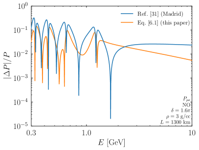
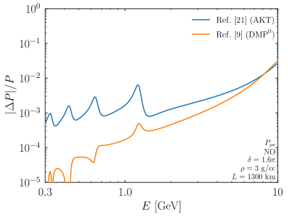
Figure 1: Left panel: We show the fractional precision for the appearance probability in Cervera et al. (2000) compared to the exact expression in blue. In orange we change $\Delta m^{2}_{31}\to\Delta m^{2}_{ee}$ which makes the expression in Cervera et al. (2000) respect all $2^{7}=128$ discrete parameter symmetries of the vacuum parameters including the 1-2 interchange and include a $c_{13}^{2}$ factor, see eq. 28. Right panel: we show the precision of AKT, Agarwalla et al. (2014), which does not respect the parameter symmetries as well as DMP, Denton et al. (2016), which does respect the parameter symmetries. In both of these panels, expressions that respect the parameter symmetries have better precision. We use the best fit oscillation parameters from de Salas et al. (2021) and $\delta=1.6\pi$ to avoid any accidental CP phase cancellations.

In fact, we found that there is generally an increase in precision when using a form that respects all the available parameter symmetries for both the simpler expressions discussed at the beginning of the section and those based on rotations in the previous papers. In fig. 1 we show the precision for the expressions from Cervera et al. (2000); Agarwalla et al. (2014); Denton et al. (2016) and eq. 28 above. We also verified that in Akhmedov et al. (2004); Friedland and Lunardini (2006) which are similar to Cervera et al. (2000), the original approximate expressions have a constant error $\sim 2\%$ as $E\to\infty$, but a change from $\Delta m^{2}_{3i}\to\Delta m^{2}_{ee}$ results in convergence at high energies for the expressions from Cervera et al. (2000); Friedland and Lunardini (2006) and generally improved precision.

VI.3 Approximations for other oscillation parameters

Another example of the impact of these parameter symmetries on the physics of neutrino oscillations is the size of the matter potential at the solar and atmospheric resonances given by

$$a^{R}_{\text{sol}} \approx\cos 2\theta_{12}\Delta m^{2}_{21}/\cos^{2}\theta_{13}$$

$$\text{and}\quad a^{R}_{\text{atm}} \approx\cos 2\theta_{13}\Delta m^{2}_{ee}$$ (31)

respectively. These expression are both extremely accurate as fractional corrections to these expressions are of order Parke (2021)

$${\cal O}(s^{4}_{13},~{}s^{2}_{13}(\Delta m^{2}_{21}/\Delta m^{2}_{ee}),~{}(\Delta m^{2}_{21}/\Delta m^{2}_{ee})^{2})\,.$$ (32)

The above expressions for the matter potential at the resonances satisfy all the parameter symmetries including the 1-2 symmetries. Note for the atmospheric resonance it is $\Delta m^{2}_{ee}$, not $\Delta m^{2}_{31}$ or $\Delta m^{2}_{32}$ that appears, as the approximation is best when the 1-2 interchange symmetry is respected.

The Jarlskog invariant in matter is the coefficient of the $\mathcal{O}(L^{3})$ term in the appearance probability, and can also be simply approximated as Denton and Parke (2019)

$$\widehat{J} \approx\frac{J}{\mathcal{S}_{\odot}\mathcal{S}_{\rm atm}}\,,$$ (33)

$$\mathcal{S}_{\odot} \equiv\sqrt{(\cos 2\theta_{12}-c_{13}^{2}a/\Delta m^{2}_{21})^{2}+\sin^{2}2\theta_{12}}\,,$$ (34)

$$\mathcal{S}_{\rm atm} \equiv\sqrt{(\cos 2\theta_{13}-a/\Delta m^{2}_{ee})^{2}+\sin^{2}2\theta_{13}}\,.$$ (35)

Each of these terms respects all the symmetries, and if $\Delta m^{2}_{ee}$ is changed to $\Delta m^{2}_{31}$ or $\Delta m^{2}_{32}$ which do not respect these parameter symmetries, the precision of the approximation is a factor $\gtrsim 10$ times worse.

The effective $\Delta m^{2}$’s for disappearance experiments in vacuum are given by

$$\Delta m^{2}_{ee} =\cos^{2}\theta_{12}\Delta m^{2}_{31}+\sin^{2}\theta_{12}\Delta m^{2}_{31}\,,$$ (36)

$$\Delta m^{2}_{\mu\mu} \approx\sin^{2}\theta_{12}\Delta m^{2}_{31}+\cos^{2}\theta_{12}\Delta m^{2}_{31}$$

$$+2\sin\theta_{23}\cos\theta_{23}\sin\theta_{13}\sin\theta_{12}\cos\theta_{12}$$

$$\times~{}\Delta m^{2}_{21}\cos(\delta_{12}+\delta_{13}+\delta_{23})/\cos^{2}\theta_{23}\,,$$ (37)

$$\Delta m^{2}_{\tau\tau} \approx\sin^{2}\theta_{12}\Delta m^{2}_{31}+\cos^{2}\theta_{12}\Delta m^{2}_{31}$$

$$-2\sin\theta_{23}\cos\theta_{23}\sin\theta_{13}\sin\theta_{12}\cos\theta_{12}$$

$$\times~{}\Delta m^{2}_{21}\cos(\delta_{12}+\delta_{13}+\delta_{23})/\sin^{2}\theta_{23}\,,$$ (38)

for $\nu_{e}$, $\nu_{\mu}$ and $\nu_{\tau}$ disappearance respectively Nunokawa et al. (2005). Each of these satisfies the symmetries given in section II for (12), (13), and (23) sectors independently. Similarly, ref. Zhou (2017) found that the eigenvalues in matter can be better approximated by using an atmospheric mass splitting of either $\Delta m^{2}_{ee}$ or $\frac{1}{2}(\Delta m^{2}_{31}+\Delta m^{2}_{32})$, both of which respect the above parameter symmetries, over other possible definitions which may not respect these parameter symmetries.

Finally, we note that the relevant exact and approximate two-flavor $\Delta m^{2}$ and mixing angle for $\nu_{e}$ disappearance in matter Denton and Parke (2018),

$$\Delta\widehat{m^{2}}_{ee} =\widehat{m^{2}}_{3}-(\widehat{m^{2}}_{1}+\widehat{m^{2}}_{2})$$

$$-[m^{2}_{3}-(m^{2}_{1}+m^{2}_{2})]+\Delta m^{2}_{ee}\,,$$ (39)

$$\Delta\widetilde{m^{2}}_{ee} =\Delta m^{2}_{ee}\mathcal{S}_{\rm atm}\,,\text{ and }\sin 2\widetilde{\theta}_{13}=\frac{\sin 2\theta_{13}}{\mathcal{S}_{\rm atm}}\,,$$ (40)

also respect all of the above symmetries, and that other possible forms that don’t respect these symmetries are less precise.

VII Conclusions

The PDG Zyla et al. (2020) parameterization of the lepton mixing matrix of three rotations has been the de facto standard parameterization for neutrino oscillations for many years now. This parameterization has many favorable phenomenological properties Denton and Pestes (2021), but it also leaves open many parameter symmetries. These parameter symmetries relate two seemingly different sets of parameters to the same underlying physics, such as $\theta_{13}=8.5^{\circ}$ and $\theta_{13}=171.5^{\circ}$. In this paper we elucidate what these parameter symmetries are in the context of changing signs of $\sin\theta_{ij}$ or $\cos\theta_{ij}$ and adjusting the appropriate complex phase adjustment. These parameter symmetries then allow one to define the mixing angles as within a range spanning $\pi/2$ radians subject to certain restrictions, typically taken to be $\theta_{ij}\in[0,\pi/2)$. In addition, these parameter symmetries allow one to either fix $\Delta m^{2}_{21}>0$ or $\theta_{12}\in[0,\pi/4)$ depending on one’s preference.

While the allowed ranges of the vacuum parameters have been previously identified, the framework presented here makes the connection to the parameter symmetries manifest, which makes it clear that the same parameter symmetries separately apply to the parameters in the presence of matter. Thus in matter one has $2^{14}=16,384$ parameter symmetries including both vacuum and matter parameters. In addition, if one uses an approximate perturbative scheme such as that in DMP Denton et al. (2016), one has nearly all of the parameter symmetries to any order in perturbation theory as well, $2^{13}=8,192$, subject to key matching conditions between the vacuum parameters and the approximate matter parameters. Finally, we note that CPT invariance leads to another factor of two in the number of symmetries for each vacuum, matter, and approximate matter expressions. All combined this paper highlights 49,408 discrete parameter symmetries which apply to both neutrino and anti-neutrino oscillations across the three different frameworks. The CPT parameter symmetry combined with one of the other discrete parameter symmetries gives rise to the well known LMA-Light – LMA-Dark degeneracy.

These parameter symmetries not only make it clear from where the restricted ranges on the parameters come from, they also provide a powerful tool when working with approximations for various physical quantities. While such approximate expressions need not satisfy any of the parameter symmetries mentioned here to be useful, these symmetries do provide an important cross check and generally leads to improved precision.

We have focused on the standard PDG parameterization of the lepton mixing matrix, but the results presented here apply to different parameterizations containing a different sequence of rotations after straightforward modifications. It may be interesting to explore connections to other parameterizations involving generators of SU(3) Merfeld and Latimer (2014); Boriero et al. (2019); Davydova and Zhukovsky (2019), four complex phases Aleksan et al. (1994), five rotations and a complex phase Emmanuel-Costa et al. (2015), the exponential of a complex matrix Zhukovsky and Melazzini (2016).

During the completion of this paper, ref. Minakata (2021) appeared on a related topic. We note that the various vacuum, matter, and perturbative parameter symmetries mentioned there are all covered in this paper. We explicitly show the connection to our work for a representative example in appendix F.

Appendix A Transformations of the rotation matrices

In this appendix we give the effects of the transformations given in section II on the rotation matrices $U_{23}$, $U_{13}$ and $U_{12}$, respectively.

The application of the parameter symmetries to the (23)-rotation,

$$\begin{pmatrix}1&&\\ &(-1)^{m}c&(-1)^{n}se^{i(\delta+(m+n)\pi)}\\ &-(-1)^{n}se^{-i(\delta+(m+n)\pi)}&(-1)^{m}c\end{pmatrix}=\begin{pmatrix}(-1)^{m}\\ &1\\ &&1\end{pmatrix}\begin{pmatrix}1&&\\ &c&se^{i\delta}\\ &-se^{-i\delta}&c\end{pmatrix}(-1)^{m}\,.$$ (41)

In this equation: $c=c_{23},s=s_{23},\delta=\delta_{23}$ with $m=m_{23},n=n_{23}$.

The application of the parameter symmetries to the (13)-rotation,

$$\begin{pmatrix}(-1)^{m}c&\quad&(-1)^{n}se^{-i(\delta+n\pi)}\\ &1\\ -(-1)^{n}se^{i(\delta+n\pi)}&&(-1)^{m}c\end{pmatrix}=\begin{pmatrix}(-1)^{m}\\ &1\\ &&1\end{pmatrix}\begin{pmatrix}c&&se^{-i\delta}\\ &1&\\ -se^{i\delta}&&c\end{pmatrix}\begin{pmatrix}1\\ &1\\ &&(-1)^{m}\\ \end{pmatrix}\,.$$ (42)

In this equation: $c=c_{13},s=s_{13},\delta=\delta_{13}$ with $m=m_{13},n=n_{13}$. The left (right) diagonal matrix commutes with $U_{23}$ ($U_{12}$ and also $M^{2}$).

The application of the parameter symmetries to the (12) rotation without the 1-2 interchange,

$$\begin{pmatrix}(-1)^{m}c&(-1)^{n}se^{i(\delta+(m+n)\pi)}&\\ -(-1)^{n}se^{-i(\delta+(m+n)\pi)}&(-1)^{m}c&\\ &&1\end{pmatrix} =\begin{pmatrix}c&se^{i\delta}\\ -se^{-i\delta}&c\\ &&1\end{pmatrix}\begin{pmatrix}(-1)^{m}\\ &(-1)^{m}\\ &&1\end{pmatrix}\,.$$ (43)

In this equation: $c=c_{12},s=s_{12},\delta=\delta_{12}$ with $m=m_{12},n=n_{12}$.

The application of the Symmetries to the (12) rotation with 1-2 interchange,

$$\begin{pmatrix}(-1)^{m}s&(-1)^{n}ce^{i(\delta+(m+n+1)\pi)}&\\ -(-1)^{n}ce^{-i(\delta+(m+n+1)\pi)}&(-1)^{m}s&\\ &&1\end{pmatrix}\begin{pmatrix}0&1\\ 1&0\\ &&1\end{pmatrix}=\begin{pmatrix}c&se^{i\delta}\\ -se^{-i\delta}&c\\ &&1\end{pmatrix}\begin{pmatrix}-(-1)^{m}e^{i\delta}\\ &(-1)^{m}e^{-i\delta}\\ &&1\end{pmatrix}\,.$$ (44)

In this equation: $c=c_{12},s=s_{12},\delta=\delta_{12}$ with $m=m_{12},n=n_{12}$. The second matrix in eq. 44 performs the $m^{2}_{1}\leftrightarrow m^{2}_{2}$ interchange.

Then, under all the parameter symmetries given in section II, we have the symmetry transformation equation for Hamiltonian in the flavor basis:

$$U_{23}U_{13}U_{12}M^{2}U^{\dagger}_{12}U^{\dagger}_{13}U^{\dagger}_{23}\Rightarrow\operatorname{diag}((-1)^{(m_{23}+m_{13})},1,1)U_{23}U_{13}U_{12}M^{2}U^{\dagger}_{12}U^{\dagger}_{13}U^{\dagger}_{23}\operatorname{diag}((-1)^{(m_{23}+m_{13})},1,1)\,.$$ (45)

Only the diagonal matrices immediately after the equal side in eqs. 41 and 42 appear in this transformation of the vacuum Hamiltonian in the flavor basis. This can also be seen directly by calculating the Hamiltonian in the flavor basis and then applying the parameter symmetries. Only the first row and column get modified by multiplication by $(-1)^{(m_{23}+m_{13})}$. An identical result to eq. 45 exists for DMP at zero order, i.e. for $V_{23}V_{13}V_{12}\Lambda V_{12}^{\dagger}V_{13}^{\dagger}V_{23}^{\dagger}$ with $(m_{23}+m_{13})$ replaced with $(\widetilde{m_{23}}+\widetilde{m_{13}})$.

Adding the matter potential to both sides of eq. 45 does not effect this result as

$$\operatorname{diag}((-1)^{(m_{23}+m_{13})},1,1)~{}A~{}\operatorname{diag}((-1)^{(m_{23}+m_{13})},1,1)=A\,.$$ (46)

Therefore, eq. 6 is valid in both vacuum and matter.

Appendix B Delta shuffle examples

In this appendix we show exactly how one relates eq. 7 to eqs. 9-11 via diagonal rephasing matrices. Recall that we drew attention to the “delta shuffle” which allows us to write the following mixing matrices in the same way

$$U_{23}(\theta_{23},\delta_{23})U_{13}(\theta_{13},-\delta_{13})U_{12}(\theta_{12},\delta_{12}) =D_{23}U_{23}(\theta_{23},\delta)U_{13}(\theta_{13},0)U_{12}(\theta_{12},0)D^{\dagger}_{23},$$ (47)

$$=D_{13}U_{23}(\theta_{23},0)U_{13}(\theta_{13},-\delta)U_{12}(\theta_{12},0)D^{\dagger}_{13},$$

$$=D_{12}U_{23}(\theta_{23},0)U_{13}(\theta_{13},0)U_{12}(\theta_{12},\delta)D^{\dagger}_{12},$$

where

$$D_{23}=\operatorname{diag}(1,e^{-i\delta_{12}},e^{+i\delta_{13}}),\quad D_{13}=\operatorname{diag}(e^{+i\delta_{12}},1,e^{-i\delta_{23}}),\quad D_{12}=\operatorname{diag}(e^{-i\delta_{13}},e^{+i\delta_{23}},1)$$ (48)

given that $\delta=\delta_{23}+\delta_{13}+\delta_{12}\mod\ 2\pi$. Note, the $D_{jk}$’s are not unique.

Appendix C Parameter symmetries in MP

In the approximation scheme of Minakata and Parke (2016) (MP), where $V_{12}=1$, Eq. 16 becomes

$$H_{\rm flav}={} \frac{1}{2E}\left[V_{23}V_{13}\Lambda V_{13}^{\dagger}V_{23}^{\dagger}\right.\left.+(U_{23}U_{13}U_{12}M^{2}U_{12}^{\dagger}U_{13}^{\dagger}U_{23}^{\dagger}+A-V_{23}V_{13}\Lambda V_{13}^{\dagger}V_{23}^{\dagger})\right]\,.$$ (49)

Applying the $2^{7}$ vacuum symmetries to $\frac{1}{2E}\left[U_{23}U_{13}U_{12}M^{2}U_{12}^{\dagger}U_{13}^{\dagger}U_{23}^{\dagger}+A\right]$ results in the phase matrix $\operatorname{diag}((-1)^{m_{23}+m_{13}},1,1)$ multiplying the both from the left and the right, whereas $\frac{1}{2E}\left[V_{23}V_{13}\Lambda V_{13}^{\dagger}V_{23}^{\dagger}\right]$ is invariant.

Applying the following symmetries for the matter variables For $\widetilde{m}_{ij},\widetilde{n}_{ij}\in\{0,1\}$:

• $(23)$: $\widetilde{c}_{23}\rightarrow(-1)^{\widetilde{m}_{23}}~{}\widetilde{c}_{23}$, $\widetilde{s}_{23}\rightarrow(-1)^{\widetilde{n}_{23}}~{}\widetilde{s}_{23}$, and $\widetilde{\delta}_{23}\rightarrow\widetilde{\delta}_{23}\pm(\widetilde{m}_{23}+\widetilde{n}_{23})\pi$,

• $(13)$: $\widetilde{c}_{13}\rightarrow(-1)^{\widetilde{m}_{13}}~{}\widetilde{c}_{13}$, $\widetilde{s}_{13}\rightarrow(-1)^{\widetilde{n}_{13}}~{}\widetilde{s}_{13}$, and $\widetilde{\delta}_{13}\rightarrow\widetilde{\delta}_{13}\pm(\widetilde{m}_{13}+\widetilde{n}_{13})\pi$,

• $(13)$: $\widetilde{c}_{13}\rightarrow(-1)^{\widetilde{m}_{13}}~{}\widetilde{s}_{13}$, $\widetilde{s}_{13}\rightarrow(-1)^{\widetilde{n}_{13}}~{}\widetilde{c}_{13}$, and $\widetilde{\delta}_{13}\rightarrow\widetilde{\delta}_{13}\pm(\widetilde{m}_{13}+\widetilde{n}_{13}+1)\pi$, plus $\lambda_{-}\leftrightarrow\lambda_{+}$,

• The two phases given in $V_{23}(\widetilde{\theta}_{23},\widetilde{\delta}_{23})V_{13}(\widetilde{\theta}_{13},-\widetilde{\delta}_{13})$ are determined from the cancellations that must occur for the MP perturbation theory, these are:

  $$\widetilde{s}_{23}\widetilde{c}_{23}e^{i\widetilde{\delta}_{23}} =s_{23}c_{23}e^{i\delta_{23}}$$

  $$\operatorname{sign}(\widetilde{c}_{23})\widetilde{c}_{13}\widetilde{s}_{13}e^{i\widetilde{\delta}_{13}}\Delta\lambda_{+-} =\operatorname{sign}(c_{23})c_{13}s_{13}e^{i\delta_{13}}\Delta m^{2}_{ee}\,.$$ (50)

  Not surprisingly, CP violation is determined by the sum of the vacuum $\delta$’s: $\delta_{23}+\delta_{13}+\delta_{12}=\delta$ as in DMP.

The above $2^{5}$ matter parameter symmetries give

$$\frac{1}{2E}\left[V_{23}V_{13}\Lambda V_{13}^{\dagger}V_{23}^{\dagger}\right]\rightarrow\operatorname{diag}((-1)^{\widehat{m}_{23}},1,1)\frac{1}{2E}\left[V_{23}V_{13}\Lambda V_{13}^{\dagger}V_{23}^{\dagger}\right]\operatorname{diag}((-1)^{\widehat{m}_{23}},1,1)\,.$$ (51)

Matching the phase of $\nu_{e}$ between the two terms leads to the constraint that $\widehat{m}_{23}=m_{23}+m_{13}$, so the total number of matter and vacuum parameter symmetries for MP perturbation theory is $2^{11}$.

Appendix D Symmetries of the exact Hamiltonian in matter

The Hamiltonian in matter was first explicitly solved in Zaglauer and Schwarzer (1988) (ZS), but the eigenvalues as written do not respect the parameter symmetries, yet the probabilities must. If we adjust the diagonal matrix by

$$M^{2}=(c^{2}_{12}m^{2}_{1}+s^{2}_{12}m^{2}_{2})\mathbb{I}+\operatorname{diag}(-s^{2}_{12}\Delta m^{2}_{21},c^{2}_{12}\Delta m^{2}_{21},\Delta m^{2}_{ee})\,,$$ (52)

then coefficients of the characteristic equation,

$$(\widehat{{m^{2}}_{i}})^{3}-A(\widehat{{m^{2}}_{i}})^{2}+B\widehat{{m^{2}}_{i}}-C=0\,,$$ (53)

where $\widehat{{m^{2}}_{i}}$ are the three eigenvalues, are

$$A =\Delta m^{2}_{ee}+(c^{2}_{12}-s^{2}_{12})\Delta m^{2}_{21}+a\,,$$ (54)

$$B =(c^{2}_{12}-s^{2}_{12})\Delta m^{2}_{21}\Delta m^{2}_{ee}-(s_{12}c_{12}\Delta m^{2}_{21})^{2}+a[c^{2}_{13}\Delta m^{2}_{ee}+(c^{2}_{12}-s^{2}_{12})\Delta m^{2}_{21}]\,,$$ (55)

$$C =-(s_{12}c_{12}\Delta m^{2}_{21})^{2}\Delta m^{2}_{ee}+a[c^{2}_{13}(c^{2}_{12}-s^{2}_{12})\Delta m^{2}_{21}\Delta m^{2}_{ee}-s^{2}_{13}(s_{12}c_{12}\Delta m^{2}_{21})^{2}]\,.$$ (56)

From eq. 17 of ZS Zaglauer and Schwarzer (1988), the shift must be accounted for in order to see that the parameter symmetries are respected. Note that $\Delta m^{2}_{ee}$, $(c^{2}_{12}-s^{2}_{12})\Delta m^{2}_{21}$, and $(s_{12}c_{12}\Delta m^{2}_{21})^{2}$ are all unchanged under the 1-2 interchange. Under this parameter symmetry the mass-squared matrix changes

$$M^{2}\Rightarrow\operatorname{diag}(-c^{2}_{12}\Delta m^{2}_{12},s^{2}_{12}\Delta m^{2}_{12},\Delta m^{2}_{ee})=\operatorname{diag}(c^{2}_{12}\Delta m^{2}_{21},-s^{2}_{12}\Delta m^{2}_{21},\Delta m^{2}_{ee})\,,$$ (57)

which leads to an identical characteristic equation, see eq. 25.

Recall that once the eigenvalues of the Hamiltonian and the eigenvalues of the principal minors of the Hamiltonian are determined, the norm of the elements of the eigenvectors (or the norm of the elements of the diagonalizing matrix, $|W_{\alpha j}|^{2}$) are determined Denton et al. (2020a, 2021) and only the relative phases between the elements of the diagonalizing matrix are to be determined. There are multiple ways to choose these relative phases and this leads to most, but not all, of the parameter symmetries discussed in this paper.

Alternatively, without using an explicit parameterization of the PMNS matrix, $U$, and using

$$M^{2}=\operatorname{diag}(m^{2}_{1},m^{2}_{2},m^{2}_{3})\,,$$ (58)

then the coefficients of the characteristic equation (eq. 53) are given by

$$A={} m^{2}_{1}+m^{2}_{2}+m^{2}_{3}+a$$ (59)

$$B={} m^{2}_{1}m^{2}_{2}+m^{2}_{2}m^{2}_{3}+m^{2}_{3}m^{2}_{1}+a\sum_{i}m^{2}_{i}(1-|U_{ei}|^{2})$$ (60)

$$C={} m^{2}_{1}m^{2}_{2}m^{2}_{3}+a\sum_{i,j,k}m^{2}_{i}m^{2}_{j}|U_{ek}|^{2}\,,\quad\text{ ((i,j,k) all different)}$$ (61)

where $|U_{\alpha i}|^{2}$’s are the fraction of the $\alpha$-flavor in the i-th mass eigenstate in vacuum, and thus invariant under all the vacuum parameter symmetries of this paper. Therefore, the eigenvalues in matter, $\widehat{m^{2}}_{i}$, are also invariant under the vacuum parameter symmetries.

In matter, the fraction of the $\alpha$-flavor in the i-th matter mass eigenstate is given by, see Denton et al. (2020a, 2021),

$$|W_{\alpha i}|^{2}= \frac{((\widehat{m^{2}}_{i})^{2}-(\xi+\chi)_{\alpha}\,\widehat{m^{2}}_{i}+(\xi\chi)_{\alpha})}{(\widehat{m^{2}}_{i}-\widehat{m^{2}}_{j})(\widehat{m^{2}}_{i}-\widehat{m^{2}}_{k})}\,,$$ (62)

with (i,j,k) all different. The sum and product of the eigenvalues of the principal minors are given by

$$(\xi+\chi)_{\alpha} =\sum_{i}m^{2}_{i}(1-|U_{\alpha i}|^{2})+\left\{\begin{array}[]{ll}0&\alpha=e\\[5.69054pt] a&\alpha=\mu,~{}\tau\end{array}\right.\quad\text{with}\quad\sum_{\alpha}(\xi+\chi)_{\alpha}=2A\,,$$ (65)

$$(\xi\chi)_{\alpha} =\sum_{i,j,k}m^{2}_{i}m^{2}_{j}|U_{\alpha k}|^{2}+\left\{\begin{array}[]{ll}0&\alpha=e\\[5.69054pt] a\sum_{i}m^{2}_{i}|U_{\tau i}|^{2}&\alpha=\mu\\[5.69054pt] a\sum_{i}m^{2}_{i}|U_{\mu i}|^{2}&\alpha=\tau\end{array}\right.\quad\text{with}\quad\sum_{\alpha}(\xi\chi)_{\alpha}=B\,.$$ (69)

Thus, all vacuum parameter symmetries are respected by the matter physical observables as well. Only the unitarity of U has been used to derive these expressions. The variables $\widehat{m^{2}}_{i}$’s and $|W_{ei}|^{2}$’s are only dependent on $m^{2}_{i}$’s and $|U_{ei}|^{2}$’s and are explicitly independent of $|U_{\mu i}|^{2}$’s and $|U_{\tau i}|^{2}$’s ($\theta_{23}$ and $\delta$ in the PDG parameterization).

For oscillation physics, the only other quantity needed is the Jarlskog in matter, $\widehat{J}$, which is related to Jarlskog in vacuum, $J$, by Naumov (1992); Harrison and Scott (2000)

$$\widehat{J}\,\Pi_{i>j}(\widehat{m^{2}}_{i}-\widehat{m^{2}}_{j}) =J\,\Pi_{i>j}(m^{2}_{i}-m^{2}_{j})\,.$$ (70)

As discussed earlier the LHS (RHS) of this equation are invariant under all matter (vacuum) parameter symmetries of this paper. Thus, all physical observables of the exact solution in uniform matter, are invariant under all parameter symmetries of both the matter variables and the vacuum variables.

Appendix E Confirmation of the perturbative conditions for DMP

Ref. Denton et al. (2016) (DMP) presented an approximation scheme for neutrino oscillations in matter based on diagonalizing “most” of the Hamiltonian via three rotations defined as a rotation of the vacuum parameters ($U_{23}(\theta_{23},\delta)$) and then diagonalizing a 2x2 submatrix twice in succession: 13 and then 12. We here confirm that the requirements for the parameter symmetries to hold are all satisfied by the details of this scheme.

For definiteness we consider NO $\Rightarrow\lambda_{1}<\lambda_{2}<\lambda_{3}$. We start with $M^{2}$ shifted as in eq. 25. Then we define the initial eigenvalues after the (23) rotation before either of the diagonalizations,

$$\lambda_{a}=a+s^{2}_{13}\Delta m^{2}_{ee}\,,\quad\lambda_{b}=(c^{2}_{12}-s^{2}_{12})\Delta m^{2}_{21}\,,\quad\lambda_{c}=c^{2}_{13}\Delta m^{2}_{ee}\,,$$ (71)

thus all parameter symmetries satisfied for $(\lambda_{a},\lambda_{b},\lambda_{c})$.

Next, after the (13) rotation we obtain the eigenvalues,

$$\lambda_{\pm} =\frac{1}{2}(a+\Delta m^{2}_{ee}\pm\Delta\lambda_{+-})\,,$$

$$\Delta\lambda_{+-} =+\sqrt{(\Delta m^{2}_{ee}\cos 2\theta_{13}-a)^{2}+(\sin 2\theta_{13}\Delta m^{2}_{ee})^{2}}\,,$$ (72)

$$\lambda_{0} =\lambda_{b}=(c^{2}_{12}-s^{2}_{12})\Delta m^{2}_{21}\,,$$

thus all parameter symmetries are also satisfied for the $(\lambda_{-},\lambda_{0},\lambda_{+})$ eigenvalues. Therefore the diagonalizing angle, $\phi\equiv\widetilde{\theta}_{13}$, given by

$$\sin^{2}\phi=\frac{\lambda_{+}-\lambda_{c}}{\lambda_{+}-\lambda_{-}}\,,$$ (73)

also satisfies all parameter symmetries. This is the point at which Minakata and Parke (2016) stops, thus the eigenvalues in that paper all respect the parameter symmetries of the vacuum parameters.

Continuing on with the framework of Denton et al. (2016), after the (12) rotation,

$$\lambda_{3} =\frac{1}{2}(a+\Delta m^{2}_{ee}+\sqrt{(\Delta m^{2}_{ee}\cos 2\theta_{13}-a)^{2}+(\sin 2\theta_{13}\Delta m^{2}_{ee})^{2}})\,,$$

$$\lambda_{2,1} =\frac{1}{2}(\lambda_{-}+\lambda_{0}\pm\Delta\lambda_{21})\,,$$ (74)

$$\Delta\lambda_{21} =+\sqrt{(\Delta m^{2}_{21}\cos 2\theta_{12}-a_{12})^{2}+(\cos^{2}\xi)(\sin 2\theta_{12}\Delta m^{2}_{21})^{2}}\,,$$

where parameter symmetry invariant quantities $a_{12}$ and $\cos^{2}\xi$ are given by:

$$a_{12} =\frac{1}{2}(a+\Delta m^{2}_{ee}-\Delta\lambda_{+-})\,,$$ (75)

$$\cos^{2}\xi =\frac{1}{2}\frac{\Delta m^{2}_{ee}+\Delta\lambda_{+-}-a\cos 2\theta_{13}}{\Delta\lambda_{+-}}\,.$$ (76)

All parameter symmetries satisfied for $(\lambda_{1},\lambda_{2},\lambda_{3})$.

In the Hamiltonian whether we chose $\Lambda=\operatorname{diag}(\lambda_{1},\lambda_{2},\lambda_{3})$ or $\Lambda=\operatorname{diag}(\lambda_{2},\lambda_{1},\lambda_{3})$ determines whether the second diagonalizing angle, $\psi\equiv\widetilde{\theta}_{12}$, is given by

$$\sin^{2}\psi\qquad{\rm or}\qquad\cos^{2}\psi=\frac{\lambda_{2}-\lambda_{0}}{\lambda_{2}-\lambda_{1}}\,.$$ (77)

Again we have the sign choices when the square root is taken.

Nothing here depends on what sign choices one has made in vacuum. However, whether $\delta_{\phi}=\delta_{13}$ or $\delta_{\phi}=\delta_{13}+\pi$ and similarly for $\delta_{\psi}$, does depend on both sets of choices. This is related to eq. 16 where in DMP $V_{23}$ is a rotation of a new angle and phase that are taken to be the same as $\theta_{23}$ and $\delta$ in vacuum, $V_{13}$ is a rotation of the angle $\phi$, and $V_{12}$ is a rotation of the angle $\psi$. This section confirms that the approximate eigenvalues that make up the $\Lambda$ matrix are invariant under all the parameter symmetries as required by the second condition.

Here we precisely quantify how the procedure carried out in DMP Denton et al. (2016) is properly generalized to take advantage of all available parameter symmetries. First, we note that it makes sense to treat $\widetilde{\theta}_{23}$ as a separate parameter from $\theta_{23}$, just like how $\phi=\widetilde{\theta}_{13}$ and $\psi=\widetilde{\theta}_{12}$ are treated as separate variables from $\theta_{13}$ and $\theta_{12}$; similarly for the $\widetilde{\delta}_{ij}$. Thus the conditions that need to be satisfied to follow the DMP procedure are

$$s_{\widetilde{23}}c_{\widetilde{23}}e^{i\widetilde{\delta}_{23}} =s_{23}c_{23}e^{i\delta_{23}}$$

$$\operatorname{sign}(c_{\widetilde{23}})c_{\phi}s_{\phi}e^{i\delta_{\phi}}\Delta\lambda_{ee} =\operatorname{sign}(c_{23})c_{13}s_{13}e^{i\delta_{13}}\Delta m^{2}_{ee}$$ (78)

$$s_{\psi}c_{\psi}e^{i\delta_{\psi}}\Delta\lambda_{21} =(|c_{\phi}c_{13}|+|s_{\phi}s_{13}|)s_{12}c_{12}e^{i\delta_{12}}\Delta m^{2}_{21}\,.$$

From these equations its clear that the new phases must satisfy

$$\widetilde{\delta}_{jk} =\delta_{jk}\mod\ \pi\,.$$ (79)

In addition, the final requirement from section III.2,

$$m_{13}+m_{23} ={m_{\phi}}+\widetilde{m}_{23}\mod\ 2\,,$$ (80)

follows from the middle condition of eq. 78 when combined with the other requirements.

Appendix F Relationship to HM21

Recently, Minakata (2021) (HM21) appeared on a related topic. All of the parameter symmetries presented in HM21 fit within our framework. To illustrate the relationship we pick one representative example containing all relevant features, Symmetry-IVB (last line of Table 1 in HM21) for which the parameter symmetry is proven through first order in perturbation theory (our result in section III.2 is correct to all orders).

Symmetry-IVB is written as the following interchanges,

$$\theta_{23}\rightarrow-\theta_{23}\,,\qquad\theta_{13}\rightarrow-\theta_{13}\,,\qquad\theta_{12}\rightarrow-\theta_{12}\,,\qquad\delta\rightarrow\delta+\pi\,,$$

$$\phi\rightarrow-\phi\,,\qquad\lambda_{1}\leftrightarrow\lambda_{2}\,,\qquad c_{\psi}\leftrightarrow\pm s_{\psi}\,,~{}~{}s_{\psi}\leftrightarrow\pm c_{\psi}\,.$$ (81)

We note that in the notation of HM21 (which matches that in DMP Denton et al. (2016) see also appendix E) $\lambda_{i}$ are the approximate matter eigenvalues of the perturbative matrix and $\phi$ ($\psi$) are $\widetilde{\theta}_{13}$ ($\widetilde{\theta}_{12}$). Care is required in translating the statement of the parameter symmetry in HM21 to that of this paper since in HM21 it is implicitly assumed that $\widetilde{\theta}_{23}$ is the same (and thus transforms the same) as $\theta_{23}$; $\widetilde{\delta}$ and $\delta$ are similarly linked. In fact, each of the $\widetilde{\delta_{ij}}$ are taken to transform the same as the corresponding $\delta_{ij}$ (although this can be written as just a single complex phase for each side given the delta shuffle).

Then this parameter symmetry with the upper signs is equivalent to our framework with the 1-2 interchange on the approximate variables, all the $m_{ij}=\widetilde{m}_{ij}=0$, and all the $n_{ij}=\widetilde{n}_{ij}=0$ except those listed here,

• for $\theta_{23}\rightarrow-\theta_{23}$, therefore $n_{23}=1$, this requires a $\pi$ be added to $\delta_{23}$,

• for $\theta_{13}\rightarrow-\theta_{13}$, therefore $n_{13}=1$, this requires a $\pi$ be added to $\delta_{13}$,

• for $\theta_{12}\rightarrow-\theta_{12}$, therefore $n_{12}=1$, this requires a $\pi$ be added to $\delta_{12}$,

thus $\delta\rightarrow\delta+\pi$ and $m_{23}+m_{13}=0$. For the approximate matter parameters, we recall that we must also modify $\widetilde{\theta}_{23}$ and that the resultant modifications to $\widetilde{\delta}$ must match the factor of $\pi$ gained for $\delta$. We have,

• for $\widetilde{\theta}_{23}\rightarrow-\widetilde{\theta}_{23}$, therefore $\widetilde{n}_{23}=1$, this requires $\pi$ be added to $\widetilde{\delta}_{23}$,

• for $\widetilde{\theta}_{13}\rightarrow-\widetilde{\theta}_{13}$, therefore $\widetilde{n}_{13}=1$, this requires $\pi$ be added to $\widetilde{\delta}_{13}$,

• $\widetilde{m^{2}_{1}}\leftrightarrow\widetilde{m^{2}_{2}}$ with $c_{\widetilde{12}}\rightarrow\pm s_{\widetilde{12}}$ and $s_{\widetilde{12}}\rightarrow\pm c_{\widetilde{12}}$ this requires $\pi$ be added to $\widetilde{\delta}_{12}$,

thus $\widetilde{\delta}\rightarrow\widetilde{\delta}+\pi$ and $\widetilde{m}_{23}+\widetilde{m}_{13}=0$. So $\delta$ and $\widetilde{\delta}$ match as they must by the choice of definition for DMP and this example satisfies our parameter symmetry requirements including the constraint given by eq. 18. For the lower signs one additionally sets $\widetilde{m}_{12}=\widetilde{n}_{12}=1$, each of which results in a factor of $\pi$ added to $\widetilde{\delta}_{12}$ and thus no change to the complex phase. We have also verified that our scheme contains all of the parameter symmetries presented in table 1 of HM21.

Since HM21 uses the same symbol for $\delta$ in vacuum and in matter it important that they agree. However, using the same symbol in vacuum and matter for $\theta_{23}$ and $\delta$ limits the number of possible discrete parameter symmetries by $2^{3}=8$ (4 for $\theta_{23}$ and 2 for $\delta$). Note that in a general perturbative framework, $\widetilde{\delta}$ and $\delta$ can differ by $\pi$. Even accounting for these parameter symmetries, there are still additional parameter symmetries unexplored in HM21 such as those including a 1-2 interchange of both vacuum and matter parameters, those without the 1-2 interchange of the matter parameters, or those which send $c_{ij}\to-c_{ij}$ (and $c_{\widetilde{ij}}\to-c_{\widetilde{ij}}$). Using a different symbol for $\theta_{23}$ in matter with its associated $\delta_{23}$ in matter, allows additional parameter symmetries. To address the maximum possible parameter symmetries one must use different symbols for matter and vacuum for all variables and associate a separate $\delta$ for each angle, even though the oscillation probabilities only depend on the sum of these $\delta$’s.

References

- Denton and Pestes (2021) P. B. Denton and R. Pestes, JHEP 05, 139 (2021), arXiv:2006.09384 [hep-ph] .
- Cabibbo (1963) N. Cabibbo, Phys. Rev. Lett. 10, 531 (1963).
- Kobayashi and Maskawa (1973) M. Kobayashi and T. Maskawa, Prog. Theor. Phys. 49, 652 (1973).
- Pontecorvo (1957) B. Pontecorvo, Zh. Eksp. Teor. Fiz. 34, 247 (1957).
- Maki et al. (1962) Z. Maki, M. Nakagawa, and S. Sakata, Prog. Theor. Phys. 28, 870 (1962).
- Zyla et al. (2020) P. A. Zyla et al. (Particle Data Group), PTEP 2020, 083C01 (2020).
- Gluza and Zralek (2001) J. Gluza and M. Zralek, Phys. Lett. B 517, 158 (2001), arXiv:hep-ph/0106283 .
- Denton (2020) P. B. Denton, (2020), arXiv:2003.04319 [hep-ph] .
- Gonzalez-Garcia et al. (2011) M. C. Gonzalez-Garcia, M. Maltoni, and J. Salvado, JHEP 05, 075 (2011), arXiv:1103.4365 [hep-ph] .
- de Gouvea et al. (2000) A. de Gouvea, A. Friedland, and H. Murayama, Phys. Lett. B 490, 125 (2000), arXiv:hep-ph/0002064 .
- Miranda et al. (2006) O. G. Miranda, M. A. Tortola, and J. W. F. Valle, JHEP 10, 008 (2006), arXiv:hep-ph/0406280 .
- Bakhti and Farzan (2014) P. Bakhti and Y. Farzan, JHEP 07, 064 (2014), arXiv:1403.0744 [hep-ph] .
- Coloma and Schwetz (2016) P. Coloma and T. Schwetz, Phys. Rev. D 94, 055005 (2016), [Erratum: Phys.Rev.D 95, 079903 (2017)], arXiv:1604.05772 [hep-ph] .
- Denton et al. (2018a) P. B. Denton, Y. Farzan, and I. M. Shoemaker, JHEP 07, 037 (2018a), arXiv:1804.03660 [hep-ph] .
- Denton et al. (2016) P. B. Denton, H. Minakata, and S. J. Parke, JHEP 06, 051 (2016), arXiv:1604.08167 [hep-ph] .
- Rodejohann and Valle (2011) W. Rodejohann and J. W. F. Valle, Phys. Rev. D 84, 073011 (2011), arXiv:1108.3484 [hep-ph] .
- Minakata et al. (2002) H. Minakata, H. Nunokawa, and S. J. Parke, Phys. Lett. B 537, 249 (2002), arXiv:hep-ph/0204171 .
- Parke (2018) S. Parke, in 28th International Symposium on Lepton Photon Interactions at High Energies (WSP, Singapur, 2018) arXiv:1801.09643 [hep-ph] .
- Zaglauer and Schwarzer (1988) H. W. Zaglauer and K. H. Schwarzer, Z. Phys. C 40, 273 (1988).
- Wolfenstein (1978) L. Wolfenstein, Phys. Rev. D 17, 2369 (1978).
- Kimura et al. (2002) K. Kimura, A. Takamura, and H. Yokomakura, Phys. Rev. D 66, 073005 (2002), arXiv:hep-ph/0205295 .
- Denton et al. (2020a) P. B. Denton, S. J. Parke, and X. Zhang, Phys. Rev. D 101, 093001 (2020a), arXiv:1907.02534 [hep-ph] .
- Barenboim et al. (2019) G. Barenboim, P. B. Denton, S. J. Parke, and C. A. Ternes, Phys. Lett. B 791, 351 (2019), arXiv:1902.00517 [hep-ph] .
- Agarwalla et al. (2014) S. K. Agarwalla, Y. Kao, and T. Takeuchi, JHEP 04, 047 (2014), arXiv:1302.6773 [hep-ph] .
- Minakata and Parke (2016) H. Minakata and S. J. Parke, JHEP 01, 180 (2016), arXiv:1505.01826 [hep-ph] .
- Denton et al. (2018b) P. B. Denton, S. J. Parke, and X. Zhang, Phys. Rev. D 98, 033001 (2018b), arXiv:1806.01277 [hep-ph] .
- Denton et al. (2020b) P. B. Denton, S. J. Parke, and X. Zhang, Phys. Lett. B 807, 135592 (2020b), arXiv:1909.02009 [hep-ph] .
- Toshev (1991) S. Toshev, Mod. Phys. Lett. A 6, 455 (1991).
- Ahmad et al. (2002) Q. R. Ahmad et al. (SNO), Phys. Rev. Lett. 89, 011301 (2002), arXiv:nucl-ex/0204008 .
- Gando et al. (2013) A. Gando et al. (KamLAND), Phys. Rev. D 88, 033001 (2013), arXiv:1303.4667 [hep-ex] .
- Farzan and Tortola (2018) Y. Farzan and M. Tortola, Front. in Phys. 6, 10 (2018), arXiv:1710.09360 [hep-ph] .
- Bhupal Dev et al. (2019) P. S. Bhupal Dev et al., SciPost 2, 001 (2019), arXiv:1907.00991 [hep-ph] .
- Schechter and Valle (1981) J. Schechter and J. W. F. Valle, Phys. Rev. D 23, 1666 (1981).
- Zhou (2020) S. Zhou, (2020), arXiv:2004.10570 [hep-ph] .
- Jarlskog (1985) C. Jarlskog, Phys. Rev. Lett. 55, 1039 (1985).
- Nunokawa et al. (2005) H. Nunokawa, S. J. Parke, and R. Zukanovich Funchal, Phys. Rev. D 72, 013009 (2005), arXiv:hep-ph/0503283 .
- Akhmedov et al. (2004) E. K. Akhmedov, R. Johansson, M. Lindner, T. Ohlsson, and T. Schwetz, JHEP 04, 078 (2004), arXiv:hep-ph/0402175 .
- Freund (2001) M. Freund, Phys. Rev. D 64, 053003 (2001), arXiv:hep-ph/0103300 .
- Cervera et al. (2000) A. Cervera, A. Donini, M. B. Gavela, J. J. Gomez Cadenas, P. Hernandez, O. Mena, and S. Rigolin, Nucl. Phys. B 579, 17 (2000), [Erratum: Nucl.Phys.B 593, 731–732 (2001)], arXiv:hep-ph/0002108 .
- Friedland and Lunardini (2006) A. Friedland and C. Lunardini, Phys. Rev. D 74, 033012 (2006), arXiv:hep-ph/0606101 .
- Arafune et al. (1997) J. Arafune, M. Koike, and J. Sato, Phys. Rev. D 56, 3093 (1997), [Erratum: Phys.Rev.D 60, 119905 (1999)], arXiv:hep-ph/9703351 .
- Asano and Minakata (2011) K. Asano and H. Minakata, JHEP 06, 022 (2011), arXiv:1103.4387 [hep-ph] .
- Parke (2016) S. Parke, Phys. Rev. D 93, 053008 (2016), arXiv:1601.07464 [hep-ph] .
- Denton and Parke (2019) P. B. Denton and S. J. Parke, Phys. Rev. D 100, 053004 (2019), arXiv:1902.07185 [hep-ph] .
- de Salas et al. (2021) P. F. de Salas, D. V. Forero, S. Gariazzo, P. Martínez-Miravé, O. Mena, C. A. Ternes, M. Tórtola, and J. W. F. Valle, JHEP 02, 071 (2021), arXiv:2006.11237 [hep-ph] .
- Abe et al. (2021) K. Abe et al. (T2K), (2021), arXiv:2101.03779 [hep-ex] .
- Parke (2021) S. J. Parke, Phys. Rev. D 103, 033003 (2021), arXiv:2012.07186 [hep-ph] .
- Zhou (2017) S. Zhou, J. Phys. G 44, 044006 (2017), arXiv:1612.03537 [hep-ph] .
- Denton and Parke (2018) P. B. Denton and S. J. Parke, Phys. Rev. D 98, 093001 (2018), arXiv:1808.09453 [hep-ph] .
- Merfeld and Latimer (2014) K. M. Merfeld and D. C. Latimer, Phys. Rev. C 90, 065502 (2014), arXiv:1412.2728 [hep-ph] .
- Boriero et al. (2019) D. Boriero, D. J. Schwarz, and H. Velten, Universe 5, 203 (2019), arXiv:1704.06139 [astro-ph.CO] .
- Davydova and Zhukovsky (2019) A. A. Davydova and K. V. Zhukovsky, Phys. Atom. Nucl. 82, 281 (2019).
- Aleksan et al. (1994) R. Aleksan, B. Kayser, and D. London, Phys. Rev. Lett. 73, 18 (1994), arXiv:hep-ph/9403341 .
- Emmanuel-Costa et al. (2015) D. Emmanuel-Costa, N. R. Agostinho, J. I. Silva-Marcos, and D. Wegman, Phys. Rev. D 92, 013012 (2015), arXiv:1504.07188 [hep-ph] .
- Zhukovsky and Melazzini (2016) K. Zhukovsky and F. Melazzini, Eur. Phys. J. C 76, 462 (2016), arXiv:1608.01248 [hep-ph] .
- Minakata (2021) H. Minakata, (2021), arXiv:2106.11472v1 [hep-ph] .
- Denton et al. (2021) P. B. Denton, S. J. Parke, T. Tao, and X. Zhang, Bull. Amer. Math. Soc. (2021), 10.1090/bull/1722, arXiv:1908.03795 [math.RA] .
- Naumov (1992) V. A. Naumov, Int. J. Mod. Phys. D 1, 379 (1992).
- Harrison and Scott (2000) P. F. Harrison and W. G. Scott, Phys. Lett. B 476, 349 (2000), arXiv:hep-ph/9912435 .