Beyond Predictions in Neural ODEs:
Identification and Interventions

Abstract

Spurred by tremendous success in pattern matching and prediction tasks, researchers increasingly resort to machine learning to aid original scientific discovery. Given large amounts of observational data about a system, can we uncover the rules that govern its evolution? Solving this task holds the great promise of fully understanding the causal interactions and being able to make reliable predictions about the system’s behavior under interventions. We take a step towards answering this question for time-series data generated from systems of ordinary differential equations (ODEs). While the governing ODEs might not be identifiable from data alone, we show that combining simple regularization schemes with flexible neural ODEs can robustly recover the dynamics and causal structures from time-series data. Our results on a variety of (non)-linear first and second order systems as well as real data validate our method. We conclude by showing that we can also make accurate predictions under interventions on variables or the system itself.

1 Introduction

Many research areas increasingly embrace data-driven machine learning techniques not only for pattern matching and prediction, but hope to leverage data for original scientific discoveries. Aiming to mimic the human scientific process, we may formulate the core task of an “automated scientist” as follows: Given observational data about a system, what are the underlying rules governing it? A key part of this quest is to determine how variables depend on each other. Causal inference has put this question at its center, making it a natural candidate to potentially surface scientific insights from data.

Within causal inference, great attention has been given to “static” settings, largely ignoring temporal aspects. Each variable under consideration is a random variable whose distribution is determined as a deterministic function of other variables—its causal parents. The structure of “which variables listen to what other variables” is typically encoded as a directed acyclic graph (DAG), giving rise to graphical structural causal models (SCM) (Pearl, 2009). SCMs have been successfully deployed both for inferring causal structure as well as estimating the strength of causal effects. A key advantage of learning a causal versus an association-based model is the ability to reason about interventions and counterfactuals on certain variables in the SCM. However, in numerous scientific fields, we are interested in systems that jointly evolve over time with dynamics governed by differential equations. In such interacting systems, the instantaneous derivative of a variable is given as a function of other variables (and their derivatives). We can thus interpret the variables (or their derivatives) that enter this function as causal parents (Mooij et al., 2013). Unlike static SCMs, this type of dependence naturally accommodates cyclic dependencies and temporal co-evolution.

The grandiose hope is that machine learning may sometimes be able to deduce true causality or true laws of nature purely from observational data, promising reliable predictions not only within the observed setting, but also under interventions. In other words, a perfectly inferred causal model generalizes well out of distribution. Such an automated scientist would undoubtedly be more powerful if we allowed it to interact with the system at hand and perform experiments. However, by focusing on the purely observational setting in this work, we avoid an ad-hoc specification of which experiments can be conducted and adhere to most current practical settings, in which algorithms are not granted the opportunity for real-world interventions. Thus, in this work we take a step towards inferring causal dependence structures from time-series data of a system that is assumed to jointly evolve according to an ODE. We start with noise-free observations in continuous time, but also provide empirical results for added observation noise, irregularly sampled time points, and real gene regulatory network data, making the following contributions:

• We start by showing that recovering the ODE from a single observed solution is ill-posed even when restricting ourselves to autonomous, linear, homogeneous systems.

• Motivated by this unidentifiability, we discuss potential regularizers that aim to enforce sparsity in the number of causal interactions and show that even the regularized problem is ill-posed for a variety of reasonable regularizers.

• To probe the relevance of these unidentifiability results empirically, we develop causal structure inference techniques from time-series data combining flexible neural ODE estimators (Chen et al., 2018) with suitable regularization techniques. Our model works for non-linear ODEs with cyclic causal structure and recovers the full ODE in special cases.

• We demonstrate the efficacy of our structure inference approach on a variety of low-dimensional (non-)linear first and second order systems, for which we can also make accurate predictions under unseen interventions. On simulated autonomous, linear, homogeneous systems we show that our approach scales to tens of variables. Finally, our method produces promising results for gene regulatory network inference on real single-cell RNA-seq data with noisy and irregular samples.

This research has potential applications in many diverse fields including biology (Pfister et al., 2019) particularly for the inference of gene-regulatory networks (Matsumoto et al., 2017; Qiu et al., 2020), robotics (Murray et al., 1994; Kipf et al., 2018) and economics (Zhang, 2005).

Related work.  There is a large body of work on the discovery of causal DAGs within the static SCM framework (see, e.g., the recent surveys by Heinze-Deml et al. (2018); Vowels et al. (2021)). Most extensions of these ideas to time-series data are based on the concept of Granger causality, where we attempt to forecast one time-series based on past values of others (Granger, 1988). We review the basic ideas and contemporary methods in Section 2.3. Typically, these methods also return an acyclic directed interaction model, though feedback of the forms $X_{t}\to X_{t+1}$ or $X_{t}\to Y_{t+1}$ and $Y_{t}\to X_{t+1}$ is allowed. Similarly to static causal discovery, inferring Granger causality often relies on traditional conditional independence tests (Malinsky & Spirtes, 2018) or score-based methods (Pamfil et al., 2020). Certain extensions of SCMs to cyclic dependence structures that retain large parts of the causal interpretation (Bongers et al., 2016) also allow for causal discovery of cyclic models (Lacerda et al., 2012; Hyttinen et al., 2012; Mooij et al., 2011). These settings differ from our framing in that they cannot model the temporal evolution of an instantaneously interacting system.

Another line of research has explored connections between (asymptotic) equilibria of differential equations and (extended) SCMs that preserve behavior under interventions (Mooij et al., 2013; Bongers & Mooij, 2018; Rubenstein et al., 2018; Blom et al., 2020). Pfister et al. (2019) focus on recovering the causal dependence of a single target variable in a system of differential equations by leveraging data from multiple heterogeneous environments. Following earlier work (Dondelinger et al., 2013; Raue et al., 2015; Benson, 1979; Ballnus, 2019; Champion et al., 2019), they focus on mass-action kinetics where the derivative of the target variable is a linear combination of up to degree one interactions of its parents. They enforce sparsity by only allowing a fixed number of such terms to be non-zero. Our work differs from the above in two key ways. First, we do not assume a semantically meaningful pre-specified parametric form of the ODEs with a small set of parameters. Second, we aim at inferring the full dynamics or causal structure of all variables at once, regardless of whether equilibria exist and without access to multiple experiments. Moreover, most previous work does not analyze the inferred system’s predictive performance under interventions.

2 Setup and Background

We start by stating our main assumption and goal for this work.

Assumption 1.

We observe the temporal evolution of $n$ real-valued variables $X^{\star}:[a,b]\to\mathbb{R}^{n}$ on a continuous time interval $a<b$, such that $X^{\star}$ is a solution of the system of ODEs

$$\begin{split}\dot{X}&=f^{\star}(X,t),\text{ for }f^{\star}\in\mathcal{F}\text{ where }\\ \mathcal{F}&:=\{f:\mathbb{R}^{n}\times[a,b]\to\mathbb{R}^{n}\,|\,f\text{ uniformly Lipschitz-continuous in $X$ and continuous in $t$}\}\,.\end{split}$$ (1)

The celebrated Picard-Lindelöf theorem guarantees the existence and uniqueness of a solution of the initial value problem (IVP) $\dot{X}=f(X,t),X(a)=x_{0}$ for all $f\in\mathcal{F}$ and $x_{0}\in\mathbb{R}^{n}$ on an interval $(a-\epsilon,a+\epsilon)$ for some $\epsilon>0$. We remark that higher-order ODEs, in particular second-order ODEs $\ddot{X}=f(X,\dot{X},t)$, can be reduced to first-order systems via $U:=(X,\dot{X})\in\mathbb{R}^{2n}$, $\dot{U}=(\dot{X},\ddot{X})=(U_{2},f(U,t)$. Hence, it suffices to continue our analysis for first-order systems. In this work we are interested in the following task

$$\text{Given $X^{\star}$, identify }f^{\star}\in\mathcal{F}.\qquad\text{{(main goal)}}$$ (2)

2.1 Causal Interpretation

In SCMs causal relationships are typically described by directed parent-child relationships in a DAG, where the causes (parents) of a variable $X_{i}$ are denoted by $pa(X_{i})\subset X$. For ODEs an analogous relationship can be described by which variables “enter into $f_{i}$”. Formally, we define the causal parents of $X_{i}$, denoted by $pa_{f}(X_{i})$, as follows: $X_{j}\in pa_{f}(X_{i})$ if and only if there exist $x_{1},\ldots,x_{j-1},x_{j+1},\ldots,x_{n}\in\mathbb{R}$ such that $f_{i}(x_{1},\ldots,x_{j-1},\bullet,x_{j+1},\ldots,x_{n}):\mathbb{R}\to\mathbb{R}$ is not constant. This notion analogously extends to second and higher order equations by defining $pa_{f}(X_{i})$ as the variables $X_{j}$ for which any (higher order) derivative of $X_{j}$ enters $f_{i}$ (in the same sense as described for first order systems).

As for static SCMs, one of the key differences between a well-performing predictive model and a causal model is that a truly causal model should enable us to make predictions about hypothetical interventions on the system. In the ODE setting, interventions can be interpreted in different ways. We will focus on the following types of interventions.

1. Variable interventions: For one or multiple $i\in\{1,\ldots,n\}$, we fix $X_{i}:=c_{i},f_{i}=0$ and replace every occurrence of $X_{i}$ in the arguments of the remaining $f_{j}$ with $c_{i}$ for constants $c_{i}\in\mathbb{R}$. We interpret these interventions as externally clamping certain variables to a fixed value.

2. System interventions: We replace one or multiple $f_{i}$ with $\tilde{f}_{i}$. Here we can further distinguish between causality preserving system interventions in which the causal parents remain the same before and after the intervention, i.e., $pa_{f}(X_{i})={pa}_{\tilde{f}}(X_{i})$ for all $i$, and others.

While variable interventions closely mimic atomic interventions in the SCM sense, system interventions are of a fundamentally different nature. In SCMs we typically expect the structural equations to capture invariant mechanisms interpreted as natural laws that can and should not be altered (Bühlmann et al., 2020). Despite the plausibility of this viewpoint, we argue that in dynamical systems interventions on the system parameters can make sense. For example, imagine a chemical reaction, described by parameters for temperature-dependent reaction rates. Having observed the system at temperature $T_{1}$ where it follows $f_{T_{1}}$, it appears more natural to view a hypothetical experiment at temperature $T_{2}$ as an intervention $f_{T_{1}}\to f_{T_{2}}$ rather than adding temperature as a variable into the ODE system. We will analyze variable interventions in (non-linear) ODEs and simple system interventions primarily in linear systems where we can identify interpretable system parameters like in the chemical reaction example. Next, we briefly recap one of the key tools we build upon in this work.

2.2 (Neural) Ordinary Differential Equations

In neural ODEs (NODE) a machine learning model (often a neural network with parameters $\theta$) is used to learn the function $f_{\theta}\approx f$ from data (Chen et al., 2018). Starting from the initial observation $X^{\star}(a)$, an explicit iterative ODE solver is applied to predict $X^{\star}(t)$ for $t\in(a,b]$ using the current derivative estimates from $f_{\theta}$. The parameters $\theta$ are then updated via backpropagation on the mean squared error between predictions and observations. Unlike residual neural networks which can be seen as an Euler discretization of a continuous evolution, NODEs can make predictions for arbitrary time points. A variant of NODEs for second order systems called SONODE that essentially simply exploits the common reduction to first order systems was proposed by Norcliffe et al. (2020). They estimate the initial values $\dot{X^{\star}}(a)$ with a neural network from $X^{\star}$ in an end-to-end fashion.

The methods proposed in this paper build on the public SONODE implementation. We note that extensions to irregularly-sampled ODEs (Rubanova et al., 2019), stochastic DEs (Li et al., 2020; Oganesyan et al., 2020), partial DEs (Sun et al., 2019), Bayesian NODEs (Dandekar et al., 2020), and delay ODEs (Zhu et al., 2021) can be used directly instead of SONODEs in our method, which directly benefits from general advances in NODE modelling. As discussed extensively in the literature, NODEs can outperform traditional ODE parameter inference techniques in terms of reconstruction error, especially for non-linear $f$ (Chen et al., 2018; Dupont et al., 2019), due to the universal approximation properties of neural networks. A subsequent advantage over previous methods is that we need not pre-specify a parameterization of $f$ in terms of a small set of semantically meaningful parameters such as the constant coefficients in mass-action-kinetics.

2.3 Granger Causality

Granger causality is a classic method for causal discovery in time series data that primarily exploits the fact that “causality cannot work against time” (Granger, 1988). Informally, a time series $X_{i}$ Granger causes another time series $X_{j}$ if predicting $X_{j}$ becomes harder when excluding the values of $X_{i}$ from a universe of all time series. Assuming that $X$ is stationary, multivariate Granger causality analysis usually fits a vector autoregressive model

$$X(t)=\sum_{\tau=0}^{k}W^{(\tau)}X(t-\tau)+E(t),$$ (3)

where $E(t)\in\mathbb{R}^{n}$ is a white Gaussian random vector, $k$ is a pre-chosen maximum time lag, and we seek to infer $W^{(\tau)}\in\mathbb{R}^{n\times n}$ which govern the dynamics. In this setting, we call $X_{i}$ a Granger cause of $X_{j}$ if $|W^{(\tau)}_{i,j}|>0$ for some $\tau\in\{0,\ldots,k\}$. We need to ensure that $W^{(0)}$ encodes an acyclic dependence structure to avoid circular dependencies at the current time. Pamfil et al. (2020) consequently estimate the parameters in eq. 3 via

$$\min_{W}\bigl{\|}X(t)-\sum_{\tau=0}^{k}W^{(\tau)}X(t-\tau)\bigr{\|}_{2}+\lambda_{0}\|W^{(0)}\|_{1,1}+\lambda_{\backslash 0}\|W^{(\backslash 0)}\|_{1,1}$$ (4)

where $W=(W^{(\tau)})_{\tau=0}^{k}$, $W^{(\backslash 0)}=(W^{(\tau)})_{\tau=1}^{k}$, and $\|\cdot\|_{1,1}$ is the element-wise $\ell_{1}$ norm, which is used to encourage sparsity in the system. In addition, to ensure that the graph corresponding to $W^{(0)}$ interpreted as an adjacency matrix is acyclic, a smooth score encoding “DAG-ness” proposed by Zheng et al. (2018) is added with a separate regularization parameter. While extensions of Granger causality to nonlinear cases exist (Diks & Wolski, 2016), we will primarily compare to the described method by Pamfil et al. (2020), called Dynotears in our empirical results. This choice is motivated by the fact that the autoregressive model in eq. (3) can be viewed as a finite difference approximation to linear systems of ODEs. We describe this connection in Appendix A.

3 Theoretical Considerations

We first note that our main goal (2) is ill-posed. While a solution exists by assumption, it may not be unique, violating one of the three Hadamard properties for well-posed problems.

Proposition 1.

Under Assumption 1, the main goal (2) is ill-posed in that there exists a non-trivial $X^{\star}:[a,b]\to\mathbb{R}^{n}$ that solves the IVP $\dot{X}=f(X,t)$, $X(a)=X^{\star}(a)$ for multiple different $f\in\mathcal{F}$.

This means that the underlying system is unidentifiable from observational data. We prove the proposition with a simple counterexample in Appendix B (where we provide all proofs), but provide some notation and background for an intuitive understanding here. First, let us restrict $\mathcal{F}$ further to autonomous, linear, homogeneous systems, common models for chemical reaction networks or simple oscillating physical systems

$$\mathcal{F}_{\mathrm{lin}}:=\{f(X)=AX\,|\,A\in\mathbb{R}^{n\times n}\}\subset\mathcal{F}\,.$$ (5)

Since every $f\in\mathcal{F}_{\mathrm{lin}}$ is uniquely determined by $A$, we can use $A$ and $f$ interchangeably. For such systems, the unique solution exists for all $t\in\mathbb{R}$ and the space of general solutions of $\dot{X}=AX$ forms an $n$-dimensional sub vector space $\mathcal{L}$ of all continuously differentiable functions from $\mathbb{R}$ to $\mathbb{R}^{n}$. For a basis $\phi_{1},\ldots,\phi_{n}$ of $\mathcal{L}$, we call $\Phi_{A}=(\phi_{1},\ldots,\phi_{n}):\mathbb{R}\to\mathbb{R}^{n\times n}$ a fundamental system of the differential equation. The solution to the IVP with $X(t_{0})=x_{0}\in\mathbb{R}^{n}$ is then simply $X(t)=\Phi_{A}(t)h$ for an $h$ such that $x_{0}=\Phi_{A}(t_{0})h$, which exists since $\Phi_{A}(t)$ has full rank for all $t$. For $A\in\mathcal{F}_{\mathrm{lin}}$, a fundamental system is simply given by $\Phi_{A}(t)=e^{At}$. Hence, our main goal restricted to $\mathcal{F}_{\mathrm{lin}}$ takes the following form: Assuming $f^{\star}(X,t)=A^{\star}X$ and without loss of generality $a=0$, can we uniquely identify $A^{\star}$ given $X^{\star}$? In other words, does $e^{At}x_{0}=e^{A^{\prime}t}x_{0}$ imply $A=A^{\prime}$? This is not the case, proving Proposition 1 even in a highly restricted setting.

The most common approach to dealing with ill-posed problems is regularization: adding further assumptions under which a unique solution will be found by a stable algorithm. For ODE parameter inference, enforcing “simplicity in the governing system” is a popular choice:

Regularized goal.  Given $X^{\star}$, find $f\in\mathcal{F}$ such that $X^{\star}$ solves $\dot{X}=f(X,t)$ and $f\in\operatorname*{arg\,min}_{g\in\mathcal{F}}\|g\|$ for some measure of complexity $\|\cdot\|:\mathcal{F}\to\mathbb{R}_{\geq 0}$.

The gap between our main goal (2) and the regularized goal can only be closed if (a) we assume that nature always chooses systems with minimal $\|f\|$, and (b) the regularizer $\|\cdot\|$ is chosen such that the regularized goal identifies a unique $f\in\mathcal{F}$. For general $f\in\mathcal{F}$ one may ask for systems with the smallest number of dependency relationships, i.e., $\|f\|$ counts how many causal parent-child relationships exist in $f$, which we write as $\|f\|_{\mathrm{causal}}:=\sum_{i=1}^{n}|pa_{f}(X_{i})|$. A straightforward way of practically approximating the non-continuity requirement in our definition of causal parents is

$$\|f\|_{\epsilon}:=\sum_{i,j=1}^{n}\bm{1}\{\|\partial_{j}f_{i}\|_{2}>\epsilon\}\>\text{for the $L_{2}$ norm }\|\cdot\|_{2}\text{ and some }\epsilon\geq 0\>.$$ (6)

For $\mathcal{F}_{\mathrm{lin}}$ this translates into sparsity in the common sense $\|A\|_{\epsilon=0}=\sum_{i,j=1}^{n}\bm{1}\{A_{ij}\neq 0\}$. Since $\|f\|_{\epsilon}$ is generally not differentiable, in practice one typically adds the entry-wise $\ell_{1}$ norm $\|A\|_{1,1}=\sum_{i,j=1}^{n}|A_{ij}|$ as a penalty term, like in eq. (4). However, the following Corollary of Proposition 1 shows that we cannot uniquely identify the system even with common sparsity enforcing regularizers.

Corollary 1.

The regularized goal does not have a unique solution with $\|f\|_{\mathrm{causal}}$. For $\mathcal{F}_{\mathrm{lin}}$, it also has no unique solution with the matrix norm $\|A\|_{1}$ or element-wise norm $\|A\|_{1,1}$ .

Other regularization schemes.  In the realm of neural ODEs, one may be tempted to enforce sparsity in the neural network parameters $\theta$ directly. While this can be a sensible regularization scheme to avoid overfitting, it does not directly translate into interpretable properties of the ODE $f_{\theta}$. For example, for commonly used fully connected, feed forward neural nets, even a sparse parameter vector $\theta$ typically leads to non-zero connections from every input to each output such that $\|f\|_{\epsilon}=n^{2}$. The “blackbox nature” of deep neural nets renders it generally difficult to translate desirable interpretable properties of $f_{\theta}$ into (differentiable) constraints on $\theta$.

Alternatively, one may model each component of $f$ by a separate neural network $f_{i,\theta_{i}}:\mathbb{R}\times\mathbb{R}^{n}\to\mathbb{R}$ with separate sets of parameters $\theta_{i}$ for each $i\in\{1,\ldots,n\}$. Stacking the outputs of all $f_{i,\theta_{i}}$ we can then train each network separately from the same NODE training signal. For such a parallel setup we can enforce sparsity via $\|f_{i}\|_{\epsilon}^{\mathrm{single}}:=\sum_{j=1}^{n}\bm{1}\{\|\partial_{j}f_{i}\|_{2}>\epsilon\}$ for each component separately. This is easy to implement in practice by enforcing sparsity directly in the first layer of each neural network, which amounts to “zeroing out” certain inputs entirely. However, this is different from our original sparsity measure for the entire system $\|f\|_{\epsilon}$ in eq. (6). The latter does allow large $\|f_{i}\|_{\epsilon}^{\mathrm{single}}$ for some components $f_{i}$ as long as the entire system is sparse. In empirical comparisons the parallel approach did not perform better while being computationally more expensive. Therefore we avoid splitting $f$ into $n$ separate networks and instead aim at describing the entire system with a single NODE network.

Summary.  In this section we have shown that our main goal (2) as well as its regularized version are ill-posed. Hence, there is a gap between predictive performance (reconstruction error of $X$) and identifying the governing system, which is required to make predictions under interventions. NODEs perform well in terms of predictive performance, but theoretically they may do so by learning a “false” system. Is that the case? We now propose meaningful regularization schemes and analyze the effect of unidentifiability empirically for a wide variety of prominent dynamical systems.

4 Method

Practical regularization.  Let us write out $f_{\theta}$ explicitly as a fully connected neural net with $L$ hidden layers parameterized by $\theta:=(W^{l},b^{l})_{l=1}^{L+1}$, with $l$-th layer weights $W^{l}$ and biases $b^{l}$

$$f_{\theta}(Y)=W^{L+1}\sigma(\ldots\sigma(W^{2}\sigma(W^{1}Y+b^{1})+b^{2})+\ldots)\>,$$ (7)

where the non-linear activation function $\sigma$ is applied element-wise. With this parameterization, we now need to approximate our desired regularization $\|f_{\theta}\|_{\mathrm{causal}}$ in terms of $\theta$. A natural candidate is $\|f_{\theta}\|_{\epsilon}$ from eq. 6 where we evaluate the partial derivatives $\partial_{j}(f_{\theta})_{i}$ via automatic differentiation and replace the $L_{2}$ norm with the $\ell_{2}$ norm for finite sequences. A major drawback of this formulation is that $\|f_{\theta}\|_{\epsilon}$ is piece-wise constant in $\theta$ a serious obstacle to gradient-based optimization.

Instead, we aim at replacing $\|f\|_{\epsilon}$ with a differentiable surrogate. Ideally, we would like to use $\ell_{1}$ regularization on the strengths of all input to output connections $j\to i$ in $f_{\theta}$. Recall that for linear activation functions $f_{\theta}$ is just a linear function $f_{\theta}(Y)=AY+b$. For simplicity, consider networks without biases ($b^{l}=0$) and $\sigma(x)=x$, where we then have $A=W^{L+1}\cdot\ldots\cdot W^{1}$. With $f_{\theta}\in\mathcal{F}_{\mathrm{lin}}$, we can directly implement a continuous $\ell_{1}$ surrogate of the desired regularizer in terms of $\theta$

$$\|\theta\|_{\mathrm{simple}}:=\|A\|_{1,1}=\|W^{L+1}\cdot\ldots\cdot W^{1}\|_{1,1}\>.$$ (8)

We then say $X_{j}\in pa_{f_{\theta}}(X_{i})$ if and only if $A_{ij}\neq 0$. When restricting ourselves to $\mathcal{F}_{\mathrm{lin}}$, using $\sigma(x)=x$ together with the above sparsity constraint is thus a viable and theoretically sound method. In this case we also recover $A$ directly from $\theta$, i.e., we can infer $f$ directly on top of the causal structure. In practice, we do not know whether $f^{\star}\in\mathcal{F}_{\mathrm{lin}}$ a-priori. Thus we should remain open to the possibility of non-linear $f^{\star}$ via non-linear activation functions $\sigma$. Then $\|\theta\|_{\mathrm{simple}}$ is not a perfect surrogate for $\|f_{\theta}\|_{\mathrm{causal}}$ anymore, because we may have $X_{j}\not\in pa_{f_{\theta}}(X_{i})$ despite $A_{ij}\neq 0$. However, since the non-linearity is always only applied element-wise, the other direction still holds: $A_{ij}=0$ implies $X_{j}\not\in pa_{f_{\theta}}(X_{i})$. Therefore, enforcing $\|\theta\|_{\mathrm{simple}}$ in the non-linear case may be overly stringent on $\|f_{\theta}\|_{\mathrm{causal}}$, but will generally still result in the desired sparsity.

Causal structure inference.  While we could read off the causal structure directly from $\theta$ via $A$ in the linear case, for non-linear $\sigma$ we validate our results by visualizing partial derivatives ${\partial_{j}(f_{\theta})_{i}}$ over time showing how each $\dot{X}_{i}$ depends on each $X_{j}$. Following the reasoning of the regularizer $\|f_{\theta}\|_{\epsilon}$ in eq. (6), we then reconstruct the causal relationships via $X_{j}\in pa_{f_{\theta}}(X_{i})$ if and only if $\sum_{k=1}^{N}|{\partial_{j}f_{i}(t_{k})}|>\epsilon$ for the $N$ observations at times $a=t_{1}<\ldots<t_{N}=b$ and some threshold $\epsilon>0$. We remark here that the choice of $\epsilon$ is sensitive to the scale of the data which may be mitigated by normalizing all data before training. Empirically we did not observe strong dependence of the inferred causal structure on the choice of $\epsilon$ for normalized data.

Summary.  We add the simple regularizer $\lambda\|\theta\|_{\mathrm{simple}}$ with a tuneable regularization parameter $\lambda$ as a proxy of $\|f_{\theta}\|_{\mathrm{causal}}$ to the loss of NODE to recover a simple $f_{\theta}$ corresponding to our regularized goal. We then devised a method to recover the causal structure from $f_{\theta}$. Section 3 has shown that we still cannot guarantee to recover $f^{\star}$ even in the realizable case (where $f^{\star}=f_{\theta}$ for some reachable $\theta$), the limit of infinite data (continuous time observations), and noise free observations. In Section 5 we will assess empirically, whether our method can still recover $f_{\theta}$ that allow us to make predictions about variable and system interventions. Possible extensions of the model to handle noisy observations generated from heterogeneous experiments are discussed in Appendix D.

5 Experiments

We now illustrate the robustness of our method for causal structure inference in several case studies. The general principles readily extend to more complex model classes. Among several methods developed for causal inference based on Granger causality (Tank et al., 2021; Hyvärinen et al., 2010; Runge et al., 2019; Amornbunchornvej et al., 2019), we compare our method to Dynotears (Pamfil et al., 2020). This choice is due to the fact that our datasets mostly contain cyclic dependencies, which cannot be represented via DAGs. Details on all settings and implementation are given in Appendix C.

Linear ODEs.  We first study second-order, homogeneous, linear ODEs with constant coefficients

$$\ddot{X}=W_{1}\dot{X}+W_{2}X.$$ (9)

We begin with $n=3$ and randomly chosen true weight matrices $W^{\star}_{1},W^{\star}_{2}$ from which we generate $X^{\star}$ using a standard ODE solver, see Appendix C. Figure 1 shows that our method is not only accurate in reconstructing $X^{\star}$, but also infers the causal graph and the true ODE system $W_{i}^{\star}$ mostly correctly. The poor performance of Dynotears may be due to cyclic dependencies in $W^{\star}_{i}$.

Table 1: Experimental results using synthetic datasets with $n\in\{10,20,50\}$, varying noise level $\sigma$, and sampling irregularity (irr). SHD is the structural Hamming distance and $\overline{\text{SHD}}$ = 1.0 - SHD.

		irr = 0.0			irr = 0.2			irr = 0.7
	dim	$\overline{\text{SHD}}$	TPR	TNR	$\overline{\text{SHD}}$	TPR	TNR	$\overline{\text{SHD}}$	TPR	TNR
$\sigma=$ 0.0	10	0.97	0.95	0.98	0.98	0.97	0.98	0.92	0.93	0.91
	20	0.92	0.82	0.97	0.84	0.72	0.88	0.86	0.75	0.89
	50	0.90	0.71	0.92	0.85	0.67	0.87	0.93	0.70	0.96
$\sigma=$ 0.1	10	0.78	0.68	0.74	0.71	0.68	0.71	0.50	0.60	0.51
	20	0.82	0.79	0.82	0.79	0.74	0.80	0.61	0.48	0.65
	50	0.86	0.65	0.90	0.89	0.59	0.93	0.86	0.68	0.89

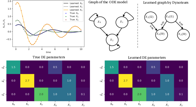
Figure 1: An example of a linear system of second-order ODEs. $li$: time lag $i$

We extend these results to study the scalability of our method and its performance when the observations are irregularly sampled (fixed fraction of observations dropped uniformly at random) with measurement noise (zero-mean Gaussian noise with standard deviation $\sigma$). The data generation process is explained in Appendix C. We evaluate the performance of the estimated graph using the structural hamming distance (SHD) (Lachapelle et al., 2019), true positive rate (TPR) and true negative rate (TNR). SHD measures the number of missing, falsely detected or reversed edges divided by the size of the adjacency matrix. The presence and absence of edges was determined by thresholding absolute values at $0.05$. The results in Table 1 (and Table 2 in Appendix E.1) show that our graph inference method performs well for non-noisy data ($\sigma=0$) and is robust to randomly removing samples from the observation. However, accuracy drops with increasing noise levels. In the noisy setting, sampling irregularities further exacerbates graph inference. The datasets and their inferred parameters are shown in Appendix E.1. As an application example of linear equations, we study a common (synthetic) chemical reaction network for transcriptional gene dynamics in Appendix E.2.

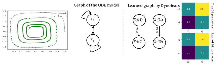
Figure 2: Results for the spiral ODE.

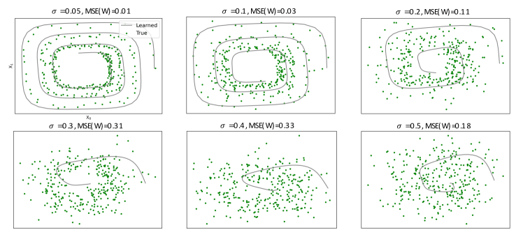
Figure 3: Results for the spiral ODE with observation noise.

Spiral ODEs.  The spiral ODE model is described by

$$\dot{X}_{0}=-\alpha{X_{0}}^{3}+\beta{X_{1}}^{3},\qquad\dot{X}_{1}=-\beta{X_{0}}^{3}+\alpha{X_{1}}^{3}$$ (10)

and features cyclic dependencies and self-loops. We follow the parameterization of the spiral ODE described by Chen et al. (2018). While Dynotears fails to infer the cyclic causal graph, Figure 2 shows that we can infer not only the causal structure, but also the actual ODE parameters $\alpha,\beta$. Again, we add Gaussian noise with different standard deviations ($0.05\leq\sigma\leq 0.5$) to analyze the robustness of our method. Figure 3 illustrates that predictive performance slowly degrades as noise levels increase. The mean-squared error (MSE) of the adjacency matrix increases substantially for $\sigma>0.2$. However, the inferred causal relationships and thus the causal graph remain correct.

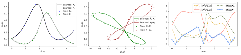
Figure 4: Results for the Lotka-Volterra predator-prey example.

Lotka-Volterra ODEs.  The Lotka-Volterra predator-prey model is given by the non-linear system

$$\dot{X}_{0}=-\alpha X_{0}-\beta X_{0}X_{1},\qquad\dot{X}_{1}=-\delta X_{1}+\gamma X_{0}X_{1}.$$ (11)

We use the same parameters as Dandekar et al. (2020). To capture the non-linearities, non-linear activation functions are required now. Figure 4 shows the excellent predictive performance (left) and the typical cyclic behavior (middle). Because of the non-linearity we cannot directly extract true parameters $A$ from network weights as in eq. (8). Instead, we perform our non-linear causal structure inference and show the partial derivatives $|\partial_{j}{f_{\theta,i}}|$ for the learned NODE network $f_{\theta}$ in Figure 4 (right). For example, from eq. (11) we know that $\partial\dot{X}_{0}/\partial X_{1}=-\beta X_{1}$ and indeed $\partial_{1}f_{\theta,0}$ in Figure 4 (right) closely resembles $X_{1}$ in Figure 4 (left) up to rescaling and a constant offset. Similarly, the remaining dependencies estimated from $f_{\theta}$ strongly correlate with the true dependencies encoded in eq. (11), giving us confidence that $f_{\theta}$ has indeed correctly identified $f^{\star}$.

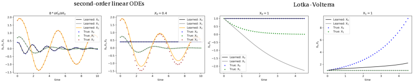
Figure 5: Predictions under system and variable interventions.

Interventions.  Next, we assess whether we can predict the behavior of a systems under interventions. To this end, we first consider the NODEs trained on observational data (without interventions) from the examples in Figures 1 and 4. Then, we apply two types of interventions: (1) a system intervention replacing one entry of $A^{\star}$ as $\tilde{A}_{00}:=8A^{\star}_{00}$ (for example, a temperature change that increases some reaction rate eightfold) in the linear setting, and (2) variable interventions $X_{0}:=0.4$ in the linear as well as $X_{0}:=1$ and $X_{1}:=1$ in the non-linear Lotka-Volterra setting (for example, keeping the number of predators fixed via culling quotas and reintroduction). In Figure 5 (left) we show that our model successfully predicts the system intervention for $X_{0}$ and its corresponding changes in $X_{2}$. Since $X_{1}$ does not depend on $X_{0}$ in this example, it remains unaffected. For the variable intervention in the linear setting, again $X_{1}$ correctly remains unaffected, while the new behavior of $X_{2}$ is prodected accurately, see Figure 5 (middle left).

In the Lotka-Volterra example, both variable interventions impact the other variable. Fixing either the predator or prey population should lead to an exponential increase or decay of the other, depending on whether the fixed levels can support higher reproduction than mortality. Figure 5 (right) shows that our method correctly predicts an exponential decay (increase) of $X_{0}$ ($X_{1}$) for fixed $X_{1}:=1$ ($X_{0}:=1$) respectively. The quantitative differences between predicted and true values are due to the exponentials quickly amplifying even small inaccuracies in the inferred parameters.

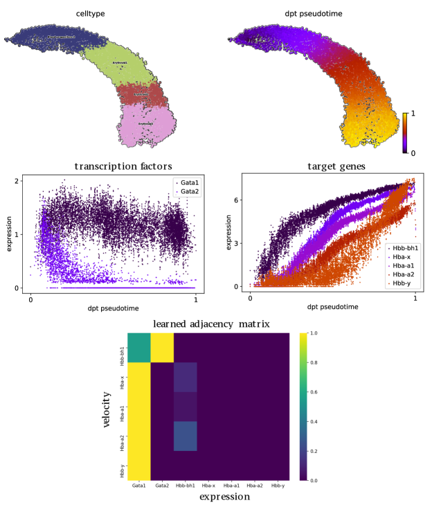
Figure 6: Gene regulatory network inference using real single-cell RNA-seq data.

Real single-cell RNA-seq data.  Finally, we apply our method for gene regulatory network inference from real mouse single-cell RNA-seq data from (Pijuan-Sala et al., 2019) (GEO accession number: GSE87038). We select a branch of data in which blood progenitors differentiate into Erythroid cells with a total of 9,192 cells (or samples). The count matrix is normalized to one million counts per cell. Figure 6 shows a UMAP representation of the data where each point corresponds to a cell colored by cell type (left) and an inferred continuous pseudotime (right). This pseudotime aims at identifying how far a cell has advanced in the differentiation process and is inferred via a diffusion map based manifold learning technique called dpt (Haghverdi et al., 2016) on 2,000 highly variable genes (Wolf et al., 2018; Bergen et al., 2020; McInnes et al., 2018). We now take measured gene expression levels over pseudotime $t$ as our observations $X^{\star}(t)$. In this setting, domain knowledge asserts that Gata genes (Gata1, Gata2) regulate the expression of hemoglobin $\alpha$ (Hba) and $\beta$ (Hba) subunits (Ding et al., 2010; Johnson et al., 2002; Suzuki et al., 2013; Shearstone et al., 2016). The normalized expression of genes related to these subunits over pseudotime is presented in Figure 6. We randomly subset 300 cells from all 9,192 as training data for our method. The expressions are scaled between 0 and 1 for each gene before training. Finally, the bottom row of Figure 6 shows the row-wise normalized absolute values of the inferred adjacency matrix. Our approach properly assigns hemoglobin subunit changes to Gata genes, particularly Gata1. Note that this dependence on Gata is inferred correctly, even though visually, the evolution of hemoglobin target genes appear to be much more correlated among themselves than with the Gata drivers. We hypothesize that the seeming independence of Gata2 is due to delays between transcription factor changes and target gene responses. Hence, extending our method to delay-ODEs is an interesting direction for future work. The predictions of our method are presented in Figure 11. The partial derivatives in Figure 12 indicate that—despite non-linear activation functions—the associations are mostly linear for the target genes except for Hbb-y. This may indicate that assuming linearity $f^{\star}\in\mathcal{F}_{\mathrm{lin}}$ can indeed be a decent approximation for certain gene regulatory networks.

6 Conclusions

In this paper, we proposed an approach to causal structure learning of dynamical systems. We show that directly inferring an ODE from a single observed solution is ill-posed, because there may exist multiple valid governing systems. Even if a method performs well in terms of predictive accuracy, it may not be able to describe the governing system or predict the behavior under interventions. Therefore, a key focus of our work lies on the predominantly neglected issue of restricting the search space in meaningful ways to be able to recover the underlying causal structure, or even the full system. Since we show that our main goal remains theoretically ill-posed even for natural sparsity enforcing regularization schemes, we probe the relevance of this issue empirically. Building on neural ODEs for learning the non-linear differential structure of dynamical systems from observational data, we devise a simple and practical method to extract causal dependencies (including cyclic relationships) from the learned derivative network. We then demonstrate how to leverage the learned structure to make predictions about different forms of interventions targeting both the evolving variables as well as parameters of the governing ODE system itself. In experiments on a range of synthetic and real-world gene regulatory settings with varying numbers of variables, noise levels, and irregular sampling intervals, we found the theoretical unidentifiability not to be a serious obstacle for reliable causal structure inference. This suggests an in-depth analysis of the conditions under which unidentifiability manifests itself in practice as a fruitful direction for future work. At the same time, extending this method for successful hypotheses generation in high-dimensional real datasets with stochasticity, delay, unobserved confounding, or heterogeneous environments is an exciting challenge for further work. Given these and other limitations, we highlight that caution must be taken when informing consequential decisions, for example in healthcare, based on causal structures learned from observational data.

Appendix A Discretization of ODE systems

For numerical treatment of derivatives in ODEs we often employ finite differences, where the derivative at time step $t$ is approximated via differences of function values at slightly different time steps. For example, the backward finite difference for the first derivative is given by $(f(t)-f(t-h))/h$ for some $h>0$. For time series data, we often use (without loss of generality) $h=1$ and can thus approximate the derivative via $f(t)-f(t-1)$. Similar approximations of higher order derivatives require more terms. Generally, to approximate the $k$-th derivative, information from $k+1$ different time points is needed. Hence, finite combinations of the form

$$\sum_{\tau=0}^{k}W_{\tau}f(t-\tau)\>,$$ (12)

which is also used by Dynotears, can in principle encode (linear combinations of) derivatives of $f$ at time $t$ up to order $k-1$. Hence, time-series based methods such as Dynotears could in principle be expected to be able to model ODE systems correctly.

Appendix B Proofs

Here, we recall and prove the statements from the main text.

B.1 Unidentifiability

See 1

Proof.

Non-uniqueness of $A$ amounts to the existence of $B\in\mathbb{R}^{n\times n}$ different from $A$ such that $\Phi_{A}h=\Phi_{B}g$ for some $g,h\in\mathbb{R}^{n}$ with $\Phi_{A}(0)h=\Phi_{B}(0)g=X(0)$. For $n=2$, $X(0):=(1,1)$ and

$$A=\begin{pmatrix}1&0\\ 0&1\end{pmatrix},\qquad B=\begin{pmatrix}0&1\\ 1&0\end{pmatrix}$$ (13)

we have $X(t)=e^{At}h=e^{Bt}g=(e^{t},e^{t})$ for all $t\in\mathbb{R}$. ∎

Remarks.  First, we note that this result appears intuitive when writing out the two systems, showing that we can choose any constant initial value $X(0)=(\alpha,\alpha)$. More broadly, any two similar matrices $A,B$ (that is, there exists an invertible matrix $U\in\mathrm{Gl}(n)$ such that $B=UAU^{-1}$) yield the same solution space up to a constant linear invertible transformation. Therefore, any system in $\mathcal{F}_{\mathrm{lin}}$ is determined up to this equivalence by its Jordan normal form, implying that Proposition 1 is not just due to isolated adversarially chosen examples. Finally, most results discussed here also hold for inhomogeneous, autonomous, linear systems ($f(X)=AX+b$ for $b\in\mathbb{R}^{n}$). In this case, the $n$-dimensional solution vector space is an affine subspace $\mathcal{L}+\tilde{X}$, where $\mathcal{L}$ is the solution vector space of the homogeneous system and $\tilde{X}$ is any specific solution of the inhomogeneous one.

B.2 Unidentifiability Despite Regularization

See 1

Proof.

We begin again with the example from eq. (13), where the matrices $A$ and $B$ have equal values for $\|\cdot\|_{\mathrm{causal}}$, $\|A\|_{1}$, and $\|A\|_{1,1}$. Let $C\in\mathbb{R}^{2\times 2}$ be any system that has $X(t)=(e^{t},e^{t})$ as a solution for the initial value $X(0)=(1,1)$ on all of $\mathbb{R}$. Since $X_{1}=X_{2}=\dot{X}_{1}=\dot{X}_{2}$ on $\mathbb{R}$ the coefficients in each row of $C$ must sum up to $1$. Hence, the minimum achievable value for $\|C\|_{1,1}=\sum_{i,j=1}^{2}|C_{ij}|$ is 2, which is achieved by both $A$ and $B$. Similarly, the minimum achievable value for $\|C\|_{1}=\max_{j=1,2}\sum_{i=1}^{2}|C_{ij}|=\max\{|C_{11}|+|C_{21}|,|C_{12}|+|C_{22}|\}$ under the row-unit-sum constraint is 1, which is also achieved by both $A$ and $B$. Finally, in the linear case the minimum achievable $\|C\|_{\mathrm{causal}}=\|C\|_{\epsilon=0}=\sum_{i,j=1}^{2}\bm{1}\{C_{ij}\neq 0\}$ is also 1, again achieved by both $A$ and $B$. Therefore, the systems $A$ and $B$ in eq. (13) are indeed among the minimum complexity solutions under all considered regularization schemes. ∎

Remarks.  Our focus lies on sparsity enforcing regularization motivated by $\|\cdot\|_{\mathrm{causal}}$ throughout. While other types of regularization may yield unique solutions (Tikhonov regularization for ill-posed problems), these typically clash with the explicit demand for sparsity in the system, with many relationships not just being weak, but desired to be non-existent. We also remark the close resemblance of our arguments to the fact that Ridge regularization yields unique solutions in linear regression whereas Lasso may not. In our example, consider $\|\cdot\|_{2}$ or $\|\cdot\|_{2,2}$ instead. In this case the minimum complexity system is uniquely given by $C_{ij}=0.5$ for $i,j\in\{1,2\}$. It is important to recognize though that this argument does not suffice to prove that our statement does not hold for these regularizers. It merely illustrates that our examples and proof techniques fail for these regularizers. Refining these unidentifiability results is an interesting direction for future work.

Appendix C Implementation Details

C.1 Synthetic Data Generation

We generate random datasets with 10, 20, and 50 variables and at most 200 observations. For each dataset, we first start with a random ground truth adjacency matrix and generate the discrete observations using off-the-shelf explicit numerical Runge-Kutta style ODE solvers (Jones et al., 2001). We then add zero-mean, fixed-variance Gaussian noise to each variable and observation independently. Finally, a percentage of samples (denoted by ‘irr’) is randomly dropped from the dataset to simulate irregular observation times.

C.2 Architecture and Training Procedure

All neural networks used in this work are fully connected, feed-forward neural networks. The initial velocities are predicted using a neural network with two hidden layers with 20 neurons each and $\tanh$ activations. The main architecture to infer velocities (or accelerations) also contains two hidden layers of sizes 20, 50, or 100 depending on the size of the input and ELU (or for some experiments linear) activation function. ELU and $\tanh$ were used because they allow for negative values in the ODE (Norcliffe et al., 2020). As an ODE solver, we use an explicit $5$-th order Dormand-Prince solver commonly denoted by dopri5.

All models are optimized using Adam (Kingma & Ba, 2017) with an initial learning rate of $0.01$. We use PyTorch’s default weight initialization scheme for the weights and set the regularization parameter $\lambda$ for the L1 penalty to $0.01$ in the 10, and 20-dimensional examples and to $0.1$ for the 50-dimensional example. All models can be trained entirely on CPUs on consumer grade Laptop machines within minutes or hours.

Appendix D Extensions

D.1 Measurement noise

Considering a deterministic version of dynamical systems with measurement noise, we have:

$$\tilde{X}(t)=X(t)+E(t).$$ (14)

Where, $X(t)$ is assumed to be governed by the ODE system and the noises $E_{i}$ are assumed to be jointly independent with zero mean. We show that our causal inference model based on NODEs can be relatively resistant to measurement noise (see the example in Figure 3). However, we can still extend our approach to latent-variable models for more complicated systems. In a general form, consider a (generative) model $e$ which encodes the initial position $\tilde{X_{0}}$ into the latent variable $Z_{0}$ as follows:

$$\mathbf{Z_{0}}=e(\mathbf{\tilde{X}},\theta_{e}).$$ (15)

This is then used by the ODE function $f$ and the ODE solver consequently:

$$\begin{array}[]{c}\dot{Z}=f(Z,t,\theta)\\ Z_{0},\ldots,Z_{N}=ODESolver(f,\mathbf{Z_{0}},(t_{0},\ldots,t_{N}))\end{array}$$ (16)

The latent variables are then decoded as follows:

$$\hat{X}_{0},\ldots,\hat{X}_{N}=d(Z,\theta_{d}).$$ (17)

Such a latent-variable model is causally interpretable and can be integrated into our method, if we can learn $\dot{X}$ as a function of $\dot{Z}$ naturally from the model. While most of the extensions to NODEs for noisy and irregularly-sampled observations perform well with respect to the reconstruction accuracy, they are hardly interpretable due to their model complexity (Rubanova et al., 2019; Norcliffe et al., 2021).

D.2 Data from Heterogeneous Systems

Our algorithm could potentially also be extended to (noisy) observations generated from heterogeneous experiments. Following Pfister et al. (2019), in this case we treat the observations from each experiments as a time-series sample. Training the model with heterogeneous samples, we may hope to identify the causal model that is invariant across the experiments (Pfister et al., 2019). It is an interesting direction for future work to determine whether heterogeneous experiments allow us to overcome the unidentifiability results in Section 3.

Appendix E Extended Results

E.1 Synthetic Linear ODEs

Table 2: Extended results using synthetic datasets with 10, 20, and 50 dimensions, varying noise level ($\sigma$) and irregularity of sampling time (irr), related to Table 1. $\overline{\text{SHD}}$ = 1.0 - SHD.

		irr = 0.0			irr = 0.2			irr = 0.5			irr = 0.7
	dim	$\overline{\text{SHD}}$	TPR	TNR	$\overline{\text{SHD}}$	TPR	TNR	$\overline{\text{SHD}}$	TPR	TNR	$\overline{\text{SHD}}$	TPR	TNR
$\sigma=$ 0.0	10	0.97	0.95	0.98	0.98	0.97	0.98	0.93	0.97	0.91	0.92	0.93	0.91
	20	0.92	0.82	0.97	0.84	0.72	0.88	0.85	0.74	0.88	0.86	0.75	0.89
	50	0.90	0.71	0.92	0.85	0.67	0.87	0.92	0.69	0.96	0.93	0.70	0.96
$\sigma=$ 0.05	10	0.88	0.81	0.92	0.87	0.80	0.92	0.86	0.84	0.88	0.67	0.48	0.87
	20	0.86	0.78	0.89	0.84	0.72	0.88	0.72	0.59	0.75	0.69	0.53	0.73
	50	0.91	0.64	0.94	0.90	0.69	0.93	0.90	0.67	0.93	0.89	0.65	0.93
$\sigma=$ 0.1	10	0.78	0.68	0.74	0.71	0.68	0.71	0.65	0.77	0.58	0.50	0.60	0.51
	20	0.82	0.79	0.82	0.79	0.74	0.80	0.68	0.53	0.74	0.61	0.48	0.65
	50	0.86	0.65	0.90	0.89	0.59	0.93	0.87	0.61	0.91	0.86	0.68	0.89

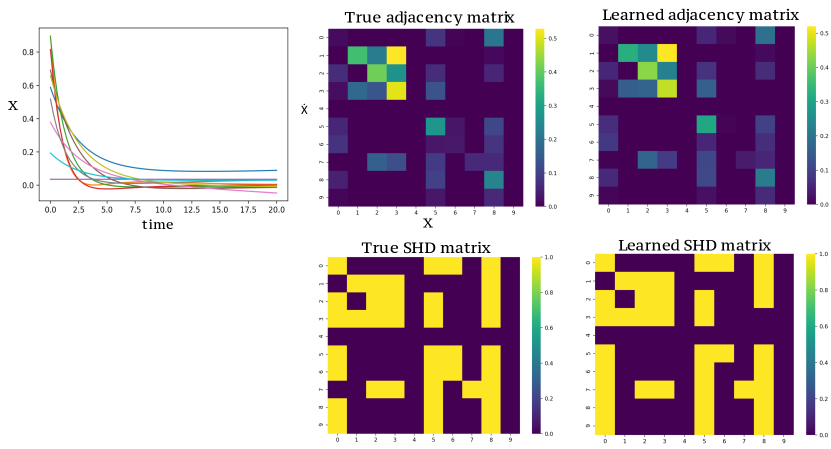
Figure 7: Synthetic data with 10 dimensions, related to Table 1.

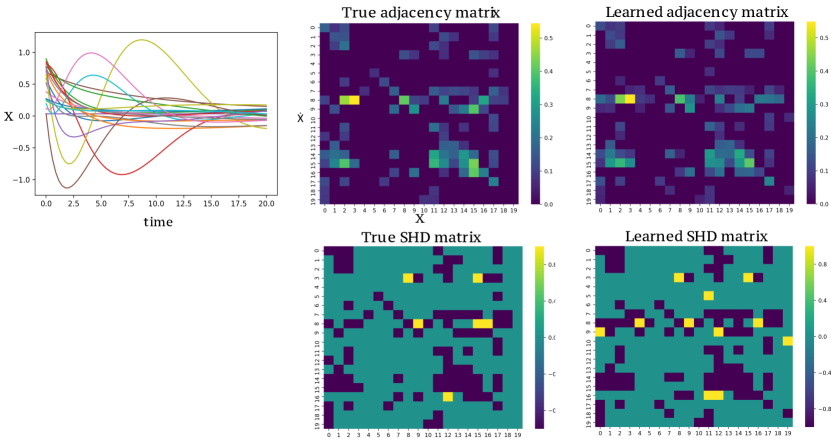
Figure 8: Synthetic data with 20 dimensions, related to Table 1. Shown are the absolute values for the adjacency matrices.

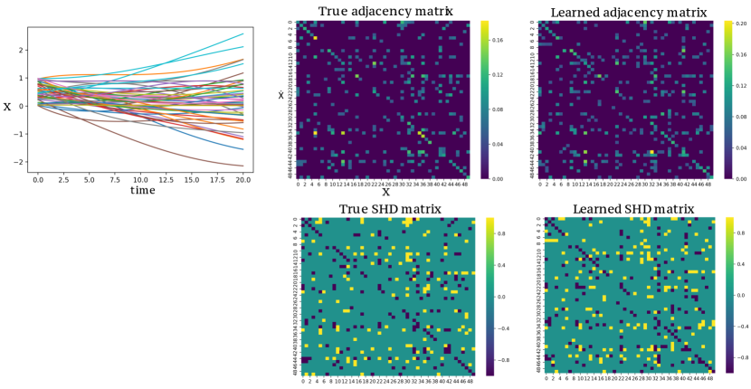
Figure 9: Synthetic data with 50 dimensions, related to Table 1. Shown are the absolute values for the adjacency matrices.

Table 2 shows the extended results (added irr $=0.5$ and $\sigma=0.05$) for the synthetic linear ODEs presented in Table 1. The synthetic datasets including their $X^{\star}$, adjacency and SHD matrices are also presented in Figures 7, 8 and 9. $S_{ij}$ in an SHD matrix represents the presence or absence of an edge between $X_{i}$ and $X_{j}$ including the sign of the effect (e.g., $S_{ij}=-1$ means $X_{j}\longrightarrow X_{i}$ with a negative coefficient). The learned adjacency matrices refer to the regularly sampled ($\mathrm{irr}=0.0$) and non-noisy ($\sigma=0$) setting.

E.2 Chemical reaction networks

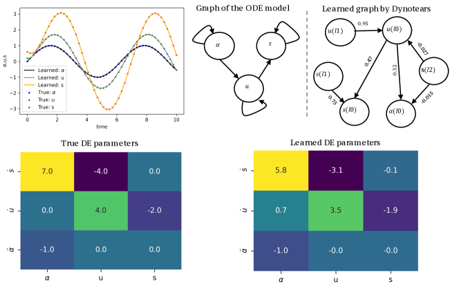
Figure 10: Example of a chemical reaction network modeling the transcriptional dynamics of a gene.

Here, we study a model of transcriptional dynamics which captures transcriptional induction and repression of unspliced precursor mRNAs $u(t)$ splicing into mature mRNAs $s(t)$ at rate $\beta$. The mature mRNAs eventually degrade with rate $\gamma$.

$$u=\alpha-\beta u,\qquad s=\beta u-\gamma s,$$ (18)

where $\alpha$ is the reaction rate of the transcription. We assume $\beta$ and $\gamma$ to be constant and the transcription rate $\alpha$ to vary over time. The results in Figure 10 show that our method can successfully learn the structural graph as well as the ODE parameters while Dynotears fails on the same task. Note that in this case we add $\alpha$ as a variable in the system with a fixed, pre-specified time-dependence in such a way that it satisfies an ODE separately from $u,s$. Our method successfully identifies this structure where the evolution of $\alpha$ does not depend on $u$ and $s$, but conversely, the derivatives of $u$ and $s$ depend on $\alpha$. Encouraged by these synthetic results, we also tested our method on real single-cell gene expression data, described in Section 5.

E.3 Gene Regulatory Network Inference

In Figure 11 and Figure 12 we show additional results for the real-data application for gene regulatory network inference from single-cell gene expression data.

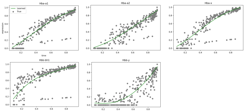
Figure 11: Predictions of the expression of the target genes together with the 300 samples used for training, related to Figure 6.

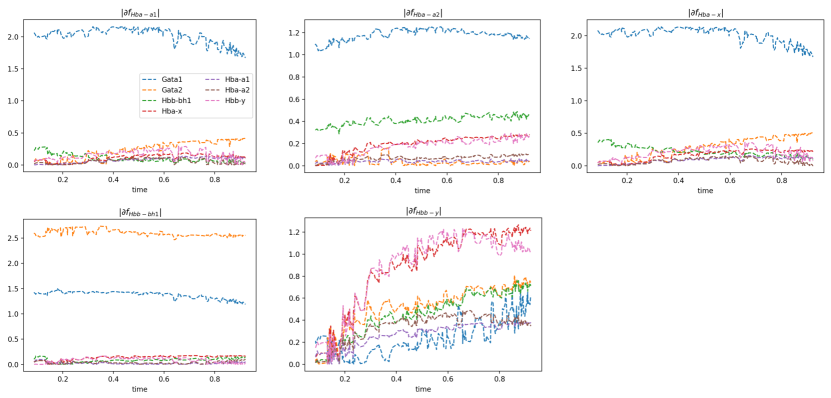
Figure 12: Gradients for the target genes, related to Figure 6.

References

- Amornbunchornvej et al. (2019) Amornbunchornvej, C., Zheleva, E., and Berger-Wolf, T. Y. Variable-lag granger causality for time series analysis. 2019 IEEE International Conference on Data Science and Advanced Analytics (DSAA), Oct 2019. doi: 10.1109/dsaa.2019.00016. URL http://dx.doi.org/10.1109/DSAA.2019.00016.
- Ballnus (2019) Ballnus, B. Development and Evaluation of Sampling-based Parameter Estimation Methods for Dynamic Biological Processes. Dissertation, Technische Universität München, München, 2019.
- Benson (1979) Benson, M. Parameter fitting in dynamic models. Ecological Modelling, 6(2):97–115, 1979. ISSN 0304-3800. doi: https://doi.org/10.1016/0304-3800(79)90029-2. URL https://www.sciencedirect.com/science/article/pii/0304380079900292.
- Bergen et al. (2020) Bergen, V., Lange, M., Peidli, S., Wolf, F. A., and Theis, F. J. Generalizing RNA velocity to transient cell states through dynamical modeling. Nature Biotechnology, 38(12), 2020. ISSN 15461696. doi: 10.1038/s41587-020-0591-3.
- Blom et al. (2020) Blom, T., Bongers, S., and Mooij, J. M. Beyond structural causal models: Causal constraints models. In Uncertainty in Artificial Intelligence, pp. 585–594. PMLR, 2020.
- Bongers & Mooij (2018) Bongers, S. and Mooij, J. M. From random differential equations to structural causal models: The stochastic case. arXiv preprint arXiv:1803.08784, 2018.
- Bongers et al. (2016) Bongers, S., Peters, J., Schölkopf, B., and Mooij, J. M. Theoretical aspects of cyclic structural causal models. arXiv preprint arXiv:1611.06221, 2016.
- Bühlmann et al. (2020) Bühlmann, P. et al. Invariance, causality and robustness. Statistical Science, 35(3):404–426, 2020.
- Champion et al. (2019) Champion, K., Lusch, B., Kutz, J. N., and Brunton, S. L. Data-driven discovery of coordinates and governing equations. Proceedings of the National Academy of Sciences, 116(45):22445–22451, 2019. ISSN 0027-8424. doi: 10.1073/pnas.1906995116. URL https://www.pnas.org/content/116/45/22445.
- Chen et al. (2018) Chen, R. T. Q., Rubanova, Y., Bettencourt, J., and Duvenaud, D. K. Neural ordinary differential equations. In Bengio, S., Wallach, H., Larochelle, H., Grauman, K., Cesa-Bianchi, N., and Garnett, R. (eds.), Advances in Neural Information Processing Systems, volume 31. Curran Associates, Inc., 2018. URL https://proceedings.neurips.cc/paper/2018/file/69386f6bb1dfed68692a24c8686939b9-Paper.pdf.
- Dandekar et al. (2020) Dandekar, R., Dixit, V., Tarek, M., García-Valadez, A., and Rackauckas, C. Bayesian neural ordinary differential equations, 2020. ISSN 23318422.
- Diks & Wolski (2016) Diks, C. and Wolski, M. Nonlinear Granger Causality: Guidelines for Multivariate Analysis. Journal of Applied Econometrics, 31(7), 2016. ISSN 10991255. doi: 10.1002/jae.2495.
- Ding et al. (2010) Ding, Y. L., Xu, C. W., Wang, Z. D., Zhan, Y. Q., Li, W., Xu, W. X., Yu, M., Ge, C. H., Li, C. Y., and Yang, X. M. Over-expression of EDAG in the myeloid cell line 32D: Induction of GATA-1 expression and erythroid/megakaryocytic phenotype. Journal of Cellular Biochemistry, 110(4), 2010. ISSN 10974644. doi: 10.1002/jcb.22597.
- Dondelinger et al. (2013) Dondelinger, F., Husmeier, D., Rogers, S., and Filippone, M. Ode parameter inference using adaptive gradient matching with gaussian processes. In Carvalho, C. M. and Ravikumar, P. (eds.), Proceedings of the Sixteenth International Conference on Artificial Intelligence and Statistics, volume 31 of Proceedings of Machine Learning Research, pp. 216–228, Scottsdale, Arizona, USA, 29 Apr–01 May 2013. PMLR. URL http://proceedings.mlr.press/v31/dondelinger13a.html.
- Dupont et al. (2019) Dupont, E., Doucet, A., and Teh, Y. W. Augmented neural ODEs, 2019. ISSN 23318422.
- Granger (1988) Granger, C. W. Some recent development in a concept of causality. Journal of Econometrics, 39(1-2), 1988. ISSN 03044076. doi: 10.1016/0304-4076(88)90045-0.
- Haghverdi et al. (2016) Haghverdi, L., Büttner, M., Wolf, F. A., Buettner, F., and Theis, F. J. Diffusion pseudotime robustly reconstructs lineage branching. Nature Methods, 13(10), 2016. ISSN 15487105. doi: 10.1038/nmeth.3971.
- Heinze-Deml et al. (2018) Heinze-Deml, C., Maathuis, M. H., and Meinshausen, N. Causal structure learning. Annual Review of Statistics and Its Application, 5:371–391, 2018.
- Hirsch & Smale (1974) Hirsch, M. and Smale, S. Differential equations, dynamical systems, and linear algebra (pure and applied mathematics, vol. 60). 1974.
- Hyttinen et al. (2012) Hyttinen, A., Eberhardt, F., and Hoyer, P. O. Learning linear cyclic causal models with latent variables. The Journal of Machine Learning Research, 13(1):3387–3439, 2012.
- Hyvärinen et al. (2010) Hyvärinen, A., Zhang, K., Shimizu, S., and Hoyer, P. O. Estimation of a structural vector autoregression model using non-gaussianity. Journal of Machine Learning Research, 11(56):1709–1731, 2010. URL http://jmlr.org/papers/v11/hyvarinen10a.html.
- Johnson et al. (2002) Johnson, K. D., Grass, J. A., Boyer, M. E., Kiekhaefer, C. M., Blobel, G. A., Weiss, M. J., and Bresnick, E. H. Cooperative activities of hematopoietic regulators recruit RNA polymerase II to a tissue-specific chromatin domain. Proceedings of the National Academy of Sciences, 99(18):11760–11765, sep 2002. ISSN 0027-8424. doi: 10.1073/PNAS.192285999. URL https://www.pnas.org/content/99/18/11760.
- Jones et al. (2001) Jones, E., Oliphant, T., Peterson, P., et al. SciPy: Open source scientific tools for Python, 2001. URL http://www.scipy.org/.
- Kingma & Ba (2017) Kingma, D. P. and Ba, J. Adam: A method for stochastic optimization, 2017.
- Kipf et al. (2018) Kipf, T., Fetaya, E., Wang, K.-C., Welling, M., and Zemel, R. Neural relational inference for interacting systems, 2018.
- Lacerda et al. (2012) Lacerda, G., Spirtes, P. L., Ramsey, J., and Hoyer, P. O. Discovering cyclic causal models by independent components analysis. arXiv preprint arXiv:1206.3273, 2012.
- Lachapelle et al. (2019) Lachapelle, S., Brouillard, P., Deleu, T., and Lacoste-Julien, S. Gradient-Based Neural DAG Learning. jun 2019. URL http://arxiv.org/abs/1906.02226.
- Li et al. (2020) Li, X., Wong, T.-K. L., Chen, R. T. Q., and Duvenaud, D. Scalable Gradients for Stochastic Differential Equations. jan 2020. URL http://arxiv.org/abs/2001.01328.
- Malinsky & Spirtes (2018) Malinsky, D. and Spirtes, P. Causal Structure Learning from Multivariate Time Series in Settings with Unmeasured Confounding. Proceedings of 2018 ACM SIGKDD Workshop on Causal Disocvery, 2018.
- Matsumoto et al. (2017) Matsumoto, H., Kiryu, H., Furusawa, C., Ko, M. S. H., Ko, S. B. H., Gouda, N., Hayashi, T., and Nikaido, I. SCODE: an efficient regulatory network inference algorithm from single-cell RNA-Seq during differentiation. Bioinformatics, 33(15):2314–2321, 04 2017. ISSN 1367-4803. doi: 10.1093/bioinformatics/btx194. URL https://doi.org/10.1093/bioinformatics/btx194.
- McInnes et al. (2018) McInnes, L., Healy, J., and Melville, J. UMAP: Uniform Manifold Approximation and Projection for Dimension Reduction. feb 2018. URL http://arxiv.org/abs/1802.03426.
- Mooij et al. (2011) Mooij, J. M., Janzing, D., Heskes, T., and Schölkopf, B. On causal discovery with cyclic additive noise models. In Shawe-Taylor, J., Zemel, R., Bartlett, P., Pereira, F., and Weinberger, K. Q. (eds.), Advances in Neural Information Processing Systems, volume 24. Curran Associates, Inc., 2011. URL https://proceedings.neurips.cc/paper/2011/file/d61e4bbd6393c9111e6526ea173a7c8b-Paper.pdf.
- Mooij et al. (2013) Mooij, J. M., Janzing, D., and Schölkopf, B. From ordinary differential equations to structural causal models: the deterministic case. arXiv preprint arXiv:1304.7920, 2013.
- Murray et al. (1994) Murray, R. M., Sastry, S. S., and Zexiang, L. A Mathematical Introduction to Robotic Manipulation. CRC Press, Inc., USA, 1st edition, 1994. ISBN 0849379814.
- Norcliffe et al. (2020) Norcliffe, A., Bodnar, C., Day, B., Simidjievski, N., and Liò, P. On Second Order Behaviour in Augmented Neural ODEs. jun 2020. URL http://arxiv.org/abs/2006.07220.
- Norcliffe et al. (2021) Norcliffe, A., Bodnar, C., Day, B., Moss, J., and Liò, P. Neural ode processes, 2021.
- Oganesyan et al. (2020) Oganesyan, V., Volokhova, A., and Vetrov, D. Stochasticity in Neural ODEs: An Empirical Study, 2020. ISSN 23318422.
- Pamfil et al. (2020) Pamfil, R., Sriwattanaworachai, N., Desai, S., Pilgerstorfer, P., Beaumont, P., Georgatzis, K., and Aragam, B. DYNOTEARS: Structure Learning from Time-Series Data. feb 2020. URL https://arxiv.org/abs/2002.00498.
- Pearl (2009) Pearl, J. Causality. Cambridge university press, 2009.
- Pfister et al. (2019) Pfister, N., Bauer, S., and Peters, J. Learning stable and predictive structures in kinetic systems. Proceedings of the National Academy of Sciences, 116(51):25405–25411, 2019.
- Pijuan-Sala et al. (2019) Pijuan-Sala, B., Griffiths, J. A., Guibentif, C., Hiscock, T. W., Jawaid, W., Calero-Nieto, F. J., Mulas, C., Ibarra-Soria, X., Tyser, R. C., Ho, D. L. L., Reik, W., Srinivas, S., Simons, B. D., Nichols, J., Marioni, J. C., and Göttgens, B. A single-cell molecular map of mouse gastrulation and early organogenesis. Nature, 566(7745), 2019. ISSN 14764687. doi: 10.1038/s41586-019-0933-9.
- Qiu et al. (2020) Qiu, X., Rahimzamani, A., Wang, L., Ren, B., Mao, Q., Durham, T., McFaline-Figueroa, J. L., Saunders, L., Trapnell, C., and Kannan, S. Inferring causal gene regulatory networks from coupled single-cell expression dynamics using scribe. Cell Systems, 10(3):265–274.e11, 2020. ISSN 2405-4712. doi: https://doi.org/10.1016/j.cels.2020.02.003. URL https://www.sciencedirect.com/science/article/pii/S2405471220300363.
- Raue et al. (2015) Raue, A., Steiert, B., Schelker, M., Kreutz, C., Maiwald, T., Hass, H., Vanlier, J., Tönsing, C., Adlung, L., Engesser, R., Mader, W., Heinemann, T., Hasenauer, J., Schilling, M., Höfer, T., Klipp, E., Theis, F., Klingmüller, U., Schöberl, B., and Timmer, J. Data2dynamics: a modeling environment tailored to parameter estimation in dynamical systems. Bioinformatics, 31(21):3558–60, 2015.
- Rubanova et al. (2019) Rubanova, Y., Chen, R. T., and Duvenaud, D. Latent ODEs for irregularly-sampled time series, 2019. ISSN 23318422.
- Rubenstein et al. (2018) Rubenstein, P. K., Bongers, S., Schölkopf, B., and Mooij, J. M. From deterministic ODEs to dynamic structural causal models. In Globerson, A. and Silva, R. (eds.), Proceedings of the 34th Conference on Uncertainty in Artificial Intelligence (UAI-18). AUAI Press, August 2018. URL http://auai.org/uai2018/proceedings/papers/43.pdf.
- Runge et al. (2019) Runge, J., Nowack, P., Kretschmer, M., Flaxman, S., and Sejdinovic, D. Detecting and quantifying causal associations in large nonlinear time series datasets. Science Advances, 5(11):eaau4996, Nov 2019. ISSN 2375-2548. doi: 10.1126/sciadv.aau4996. URL http://dx.doi.org/10.1126/sciadv.aau4996.
- Shearstone et al. (2016) Shearstone, J. R., Golonzhka, O., Chonkar, A., Tamang, D., Van Duzer, J. H., Jones, S. S., and Jarpe, M. B. Chemical inhibition of histone deacetylases 1 and 2 induces fetal hemoglobin through activation of GATA2. PLoS ONE, 11(4), 2016. ISSN 19326203. doi: 10.1371/journal.pone.0153767.
- Sun et al. (2019) Sun, Y., Zhang, L., and Schaeffer, H. NeuPDE: Neural network based ordinary and partial differential equations for modeling time-dependent data, 2019. ISSN 23318422.
- Suzuki et al. (2013) Suzuki, M., Kobayashi-Osaki, M., Tsutsumi, S., Pan, X., Ohmori, S., Takai, J., Moriguchi, T., Ohneda, O., Ohneda, K., Shimizu, R., et al. Gata factor switching from gata 2 to gata 1 contributes to erythroid differentiation. Genes to Cells, 18(11):921–933, 2013.
- Tank et al. (2021) Tank, A., Covert, I., Foti, N., Shojaie, A., and Fox, E. B. Neural granger causality. IEEE Transactions on Pattern Analysis and Machine Intelligence, pp. 1–1, 2021. ISSN 1939-3539. doi: 10.1109/tpami.2021.3065601. URL http://dx.doi.org/10.1109/TPAMI.2021.3065601.
- Vowels et al. (2021) Vowels, M. J., Camgoz, N. C., and Bowden, R. D’ya like dags? a survey on structure learning and causal discovery. arXiv preprint arXiv:2103.02582, 2021.
- Wolf et al. (2018) Wolf, F. A., Angerer, P., and Theis, F. J. SCANPY: Large-scale single-cell gene expression data analysis. Genome Biology, 2018. ISSN 1474760X. doi: 10.1186/s13059-017-1382-0.
- Zhang (2005) Zhang, W.-B. Differential equations, bifurcations, and chaos in economics. World Scientific, 2005.
- Zheng et al. (2018) Zheng, X., Aragam, B., Ravikumar, P., and Xing, E. P. DAGs with NO TEARS: Continuous Optimization for Structure Learning. mar 2018. URL http://arxiv.org/abs/1803.01422.
- Zhu et al. (2021) Zhu, Q., Guo, Y., and Lin, W. Neural delay differential equations. arXiv preprint arXiv:2102.10801, 2021.