An Entropic Method for Discrete Systems with Gibbs Entropy

Abstract

We consider general systems of ordinary differential equations with monotonic Gibbs entropy, and introduce an entropic scheme that simply imposes an entropy fix after every time step of any existing time integrator. It is proved that in the general case, our entropy fix has only infinitesimal influence on the numerical order of the original scheme, and in many circumstances, it can be shown that the scheme does not affect the numerical order. Numerical experiments on the linear Fokker-Planck equation and nonlinear Boltzmann equation are carried out to support our numerical analysis.

65L05

1 Introduction

The second law of thermodynamics, discovered more than 170 years ago, states that the direction of the thermodynamic processes is driven by a physical quantity called entropy. The importance of this law cannot be overstated, and nearly every thermodynamic model has to respect such a property. Mathematically, there are a number of formulas to represent the entropy, among which the Gibbs entropy, formulated as the integral of $f\log f$ with $f$ being the distribution function of the states, is widely used in a variety of models such as the heat equation, the Boltzmann equation, and the Fokker-Planck equation. In our discussion, we assume a finite number of states, so that the Gibbs entropy is defined by

$$\eta(\boldsymbol{f})=\sum_{i=1}^{N}f_{i}\log f_{i}\Delta v_{i},$$

where $\boldsymbol{f}=(f_{1},\ldots,f_{N})^{T}\in\mathbb{R}_{+}^{N}$ describes the distribution of the $N$ states and $\Delta v_{i}$ represents the weight of the $i$th state. The vector $\boldsymbol{f}$ is a vector function of time $t$, and we assume that it satisfies the initial value problem

(1) $$\frac{\mathrm{d}f_{i}(t)}{\mathrm{d}t}=Q_{i}(\boldsymbol{f}(t)), i=1,\dots,N,$$

$$f_{i}(0)=f_{i}^{0},$$

with the following properties:

1. conservation of mass: $\frac{\mathrm{d}}{\mathrm{d}t}\sum_{i=1}^{N}f_{i}(t)\Delta v_{i}=0$;

2. nonnegativity: $f_{i}(t)\geq 0,\ \forall 1\leq i\leq N,t\geq 0$;

3. monotonicity of entropy: $\frac{\mathrm{d}}{\mathrm{d}t}\sum_{i=1}^{N}f_{i}(t)\log f_{i}(t)\Delta v_{i}\leq 0$.

The ODE system of the form (1) appears frequently after discretizing the thermodynamic equations in space. For example, it may arise from the finite difference discretization of the heat equation and the Fokker-Planck type equation [6, 2, 10, 4]. It may also result from the discrete velocity method and the entropic Fourier method for the Boltzmann equation [7, 3].

Although the semi-discrete scheme (1) decays entropy, there is no guarantee that this property will carry over when time is discretized. In some special cases, the entropy decay can be proved for the fully discrete scheme, see for instance [1], yet it often comes at a price of using implicit schemes and is highly problem and scheme dependent. Given the importance of entropy in thermodynamic processes, it would be desirable to have a fully discrete entropic scheme that is generic (e.g., does not require a specific type of time discretization) as well as easily implementable (e.g., does not require expensive nonlinear iterations).

To bridge the above gap, we introduce an entropic scheme in this paper to achieve the following: one can apply any time discretization to the system (1) as long as it maintains the mass conservation and nonnegativity of the solution. After each time step, if the entropy goes in the wrong direction, we provide a simple fix to make it decay monotonically. Such a fix is done by a weighted average of the current solution and the solution with maximum entropy. Via numerical analysis, we show that such a fix has only a tiny effect on the order of accuracy, and in various cases, it can be proven that the order of accuracy is not affected at all. Numerical experiments on the linear Fokker-Planck equation and nonlinear Boltzmann equation will also be carried out to support our findings.

The paper is organized as follows. In Section 2, we first outline the procedure of our entropic method and summarize the main theorems of the method. The detailed proof of the theorems with some deeper understandings is illustrated in Section 3. Section 4 provides the numerical experiments, and the conclusion follows in Section 5.

2 Main results

This section outlines the overall procedure of our entropic method and lists the main results of our numerical analysis. Before stating our theorems, we introduce the notations and review some basic properties of the Gibbs entropy.

2.1 Brief review of Gibbs entropy

Due to the conservation hypothesis (P1), below we focus on the entropy functional defined by

$$H(\boldsymbol{f})=\sum_{i=1}^{N}(f_{i}\log f_{i}-f_{i})\Delta v_{i}:=\sum_{i=1}^{N}h(f_{i})\Delta v_{i},$$

with $h(x)=x\log x-x$. Note that $H(\boldsymbol{f})$ differs from $\eta(\boldsymbol{f})$ only by a constant.

Let $\boldsymbol{C}=(C,\dots,C)^{T}\in\mathbb{R}_{+}^{N}$ with

(2) $$C=\frac{\sum_{i=1}^{N}f_{i}\Delta v_{i}}{\sum_{i=1}^{N}\Delta v_{i}}.$$

We denote by $\tilde{\boldsymbol{f}}={\boldsymbol{f}}/{C}=(\tilde{f}_{1},\dots,\tilde{f}_{N})^{T}$ the normalized $\boldsymbol{f}$, then it can be checked that

(3) $$C\eta(\tilde{\boldsymbol{f}})=H(\boldsymbol{f})-H(\boldsymbol{C}).$$

Furthermore, we define the $L^{p}$ ($p=1,2$) norm and $L^{\infty}$ norm of any $\boldsymbol{f}$ as

$$\|\boldsymbol{f}\|_{p}=\left(\sum_{i=1}^{N}f_{i}^{p}\Delta v_{i}\right)^{1/p},\qquad\|\boldsymbol{f}\|_{\infty}=\max_{i}|f_{i}|.$$

Lemma 2.1.

$\boldsymbol{C}$ is the unique global minimum point of $H(\boldsymbol{f})$ for all $\boldsymbol{f}\in\mathbb{R}_{+}^{N}$ satisfying Eq. 2 with fixed $C$.

The proof of Lemma 2.1 can be done by the concavity of $\log(x)$ and Jensen’s inequality. Furthermore, a straightforward corollary of Lemma 2.1 is that, $\boldsymbol{1}=(1,\dots,1)^{T}\in\mathbb{R}_{+}^{N}$ is the unique global minimum point of $\eta(\tilde{\boldsymbol{f}})$ for all $\tilde{\boldsymbol{f}}\in\mathbb{R}_{+}^{N}$ satisfying $\|\tilde{\boldsymbol{f}}\|_{1}=\|\boldsymbol{1}\|_{1}$. To ease the notation, we use $\|\boldsymbol{1}\|_{1}=\sum_{i=1}^{N}\Delta v_{i}=V$ to denote the volume.

The notations hereafter will be focused on the relative entropy $\eta(\tilde{\boldsymbol{f}})$ and the normalized $\tilde{\boldsymbol{f}}$ for fixed $C$. One could find its relationship to entropy function $H(\cdot)$ from Eq. 3. For simplicity, we would like to omit the tilde symbol in $\tilde{\boldsymbol{f}}$, and thus the average of the components of $\boldsymbol{f}$ will be $1$ hereafter.

2.2 Main results

We assume after temporal discretization of Eq. 1, the properties (P1) and (P2) can be preserved. Specifically, if we let $\boldsymbol{f}^{n}\geq 0$ be the numerical solution at the $n$th time step, then we have

1. conservation: $\sum_{i=1}^{N}f_{i}^{n+1}\Delta v_{i}=\sum_{i=1}^{N}f_{i}^{n}\Delta v_{i}$,

2. nonnegativity: $f_{i}^{n+1}\geq 0,\ \forall 1\leq i\leq N$.

We would like to design an entropic method such that it can fulfill a discrete version of (P3) while keeping (H1) and (H2).

Our numerical scheme is based on imposing a simple entropy fix after computing the numerical solution at every time step. Suppose that $\boldsymbol{f}^{n+1}$ is computed through evolving $\boldsymbol{f}^{n}$ by one time step. If $\eta(\boldsymbol{f}^{n+1})\leq\eta(\boldsymbol{f}^{n})$, nothing needs to be done. Otherwise, we revise the solution at the $(n+1)$th time step as

(4) $$\hat{\boldsymbol{f}}^{n+1}=\boldsymbol{f}^{n+1}+\beta_{p}(\boldsymbol{1}-\boldsymbol{f}^{n+1}),$$

where $\beta_{p}\in(0,1]$ is chosen to satisfy

(5) $$\eta(\boldsymbol{f}^{n+1}+\beta_{p}(\boldsymbol{1}-\boldsymbol{f}^{n+1}))=\eta(\boldsymbol{f}^{n}).$$

This guarantees that the entropy is always non-increasing.

In most cases, such a method stabilizes the solution since it reduces both the Gibbs entropy and the $2$-norm of vectors. Therefore we are mainly concerned about the magnitude of the fixing term $\beta_{p}(\boldsymbol{1}-\boldsymbol{f}^{n+1})$, and we hope that this term does not affect the numerical convergence order of the original scheme. Generally, the error estimation of this scheme can be analyzed in the following manner

(6) $$\|\hat{\boldsymbol{f}}^{n+1}-\boldsymbol{f}(t_{n+1})\| \leq\|\hat{\boldsymbol{f}}^{n+1}-\boldsymbol{f}^{n+1}\|+\|\boldsymbol{f}^{n+1}-\boldsymbol{f}(t_{n+1})\|$$

$$\leq\|\hat{\boldsymbol{f}}^{n+1}-\boldsymbol{f}^{n+1}\|+\|\boldsymbol{f}^{n+1}-\tilde{\boldsymbol{f}}(t_{n+1})\|+\|\tilde{\boldsymbol{f}}(t_{n+1})-\boldsymbol{f}(t_{n+1})\|,$$

where $\tilde{\boldsymbol{f}}(t)$ is the solution of the problem

(7) $$\frac{\mathrm{d}\tilde{f}_{i}(t)}{\mathrm{d}t}=Q_{i}(\tilde{\boldsymbol{f}}(t)), i=1,\dots,N,$$

$$\tilde{f}_{i}(t_{n})=f_{i}^{n}, i=1,\dots,N,$$

and hence $\|\boldsymbol{f}^{n+1}-\tilde{\boldsymbol{f}}(t_{n+1})\|$ is the “one-step error” of the scheme. The last term in Eq. 6 is usually controlled by the stability of the ODE problem with respect to the initial condition. If we assume that the scheme satisfies the following consistency condition:

$$\|\boldsymbol{f}(t_{n+1})-\boldsymbol{f}^{n+1}\|\leq O(\Delta t^{s+1}),$$

then the original scheme (before our entropy fix) is a scheme of order $s$. Here our purpose is to demonstrate that the first term in the second line of Eq. 6, i.e., $\|\beta_{p}(\boldsymbol{1}-\boldsymbol{f}^{n+1})\|$, can be controlled by the second term $\|\tilde{\boldsymbol{f}}(t_{n+1})-\boldsymbol{f}^{n+1}\|$. In the ideal case, we may find a constant $C$ such that

$$\|\beta_{p}(\boldsymbol{1}-\boldsymbol{f}^{n+1})]\|\leq C\|\tilde{\boldsymbol{f}}(t_{n+1})-\boldsymbol{f}^{n+1}\|,$$

then the numerical convergence order is not affected. Hereafter, for simplicity, we would like to omit the tilde and use $\boldsymbol{f}(t_{n+1})$ to denote the solution of Eq. 7 at time $t_{n+1}$. In other words, we assume that the solution at the $n$th time step $\boldsymbol{f}^{n}$ is exact ($\boldsymbol{f}(t_{n})=\boldsymbol{f}^{n}$), so that $\boldsymbol{f}(t_{n+1})$ becomes identical to $\tilde{\boldsymbol{f}}(t_{n+1})$.

In the following theorems, we will study a stronger result

(8) $$\eta(\boldsymbol{f}^{n+1}+\beta(\boldsymbol{1}-\boldsymbol{f}^{n+1}))=\eta(\boldsymbol{f}(t_{n+1})),$$

where $\beta_{p}$ in Eq. 5 is replaced by $\beta$ and the solution at $(n+1)$th time step is revised to possess the same entropy as $\boldsymbol{f}(t_{n+1})$. Due to $\eta(\boldsymbol{f}(t_{n+1}))\leq\eta(\boldsymbol{f}^{n})$ and the monotonicity of $\eta(\boldsymbol{f}^{n+1}+\omega(\boldsymbol{1}-\boldsymbol{f}^{n+1}))$ with respect to $\omega$, we see that $\beta_{p}\leq\beta$. Therefore, it suffices to show that $\|\beta(\boldsymbol{1}-\boldsymbol{f}^{n+1})\|$ can be controlled by the difference between $\boldsymbol{f}(t_{n+1})$ and $\boldsymbol{f}^{n+1}$. Based on the commonly-used $2$-norm of vectors, we are going to prove this type of results in four different scenarios, which will be stated in the four theorems listed below.

In the first case, we have no assumptions on the structure of the solution, which may lead to a slight reduction of the numerical convergence order:

Theorem 2.2.

Given a positive and conservative numerical scheme, i.e., $\boldsymbol{f}^{n+1}\in\mathbb{R}_{+}^{N}$ and $\|\boldsymbol{f}^{n+1}\|_{1}=\|\boldsymbol{f}(t_{n+1})\|_{1}$. When $\eta(\boldsymbol{f}^{n+1})>\eta(\boldsymbol{f}^{n})$ and Eq. 8 are satisfied, if $\|\boldsymbol{f}(t_{n+1})-\boldsymbol{f}^{n+1}\|_{2}\leq 1$, then

$$\|\beta(\boldsymbol{1}-\boldsymbol{f}^{n+1})\|_{2}\leq M\|\boldsymbol{f}(t_{n+1})-\boldsymbol{f}^{n+1}\|_{2}\left(1+\left|\log\left(\|\boldsymbol{f}(t_{n+1})-\boldsymbol{f}^{n+1}\|_{2}\right)\right|\right),$$

where $M>0$ is a constant which depends on $V$, $\|\boldsymbol{f}^{n+1}\|_{\infty}$ and $\|\boldsymbol{f}(t_{n+1})\|_{\infty}$.

In this case, the right-hand side of the inequality contains a logarithmic term, which tends to infinity when $\|\boldsymbol{f}(t_{n+1})-\boldsymbol{f}^{n+1}\|_{2}$ approaches zero. However, for any $\epsilon>0$, we have

$$1+\left|\log\left(\|\boldsymbol{f}(t_{n+1})-\boldsymbol{f}^{n+1}\|_{2}\right)\right|<\|\boldsymbol{f}(t_{n+1})-\boldsymbol{f}^{n+1}\|_{2}^{-\epsilon}$$

when $\|\boldsymbol{f}(t_{n+1})-\boldsymbol{f}^{n+1}\|_{2}$ is sufficiently small, meaning that the numerical convergence order is reduced only by an arbitrary small positive number. Nevertheless, we would still like to explore the conditions under which such a logarithmic term does not exist. The remaining three cases are related to this type of results.

Intuitively, the reason of the logarithmic term in Theorem 2.2 is the unboundedness of the function $h^{\prime}(x)$ when $x$ is close to zero. In the following result, we assume that the components of the numerical solution $\boldsymbol{f}^{n+1}$ have a lower bound $C_{0}$, such that $h^{\prime}(x)$ becomes bounded:

Theorem 2.3.

Given a positive and conservative numerical scheme, i.e., $\boldsymbol{f}^{n+1}\in\mathbb{R}_{+}^{N}$ and $\|\boldsymbol{f}^{n+1}\|_{1}=\|\boldsymbol{f}(t_{n+1})\|_{1}$. When $\eta(\boldsymbol{f}^{n+1})>\eta(\boldsymbol{f}^{n})$ and Eq. 8 are satisfied, if $f^{n+1}_{i}\geq C_{0}>0$ holds for all $1\leq i\leq N$, then

$$\|\beta(\boldsymbol{1}-\boldsymbol{f}^{n+1})\|_{2}\leq M\|\boldsymbol{f}(t_{n+1})-\boldsymbol{f}^{n+1}\|_{2},$$

where $M>0$ is a constant which depends on $C_{0}$, $\|\boldsymbol{f}^{n+1}\|_{\infty}$ and $\|\boldsymbol{f}(t_{n+1})\|_{\infty}$.

The condition in this theorem disallows the numerical solution to be zero anywhere in the domain. In such a situation, if the scheme can guarantee the numerical convergence order for the $L^{\infty}$-error, we can still show that the $L^{2}$-norm of the entropy fix is small. This corresponds to our third case:

Theorem 2.4.

Given a positive and conservative numerical scheme, i.e., $\boldsymbol{f}^{n+1}\in\mathbb{R}_{+}^{N}$ and $\|\boldsymbol{f}^{n+1}\|_{1}=\|\boldsymbol{f}(t_{n+1})\|_{1}$. When $\eta(\boldsymbol{f}^{n+1})>\eta(\boldsymbol{f}^{n})$ and Eq. 8 are satisfied, if $\|\boldsymbol{f}(t_{n+1})-\boldsymbol{f}^{n+1}\|_{\infty}\leq 1/3$, it holds that

$$\|\beta(\boldsymbol{1}-\boldsymbol{f}^{n+1})\|_{2}\leq M\|\boldsymbol{f}(t_{n+1})-\boldsymbol{f}^{n+1}\|_{\infty},$$

where $M>0$ is a constant which depends on $V$, $\|\boldsymbol{f}^{n+1}\|_{\infty}$ and $\|\boldsymbol{f}(t_{n+1})\|_{\infty}$.

The last case we consider can be regarded as a generalization of Theorem 2.3. We allow the numerical solution to be small on some part of the domain, but require that the solution increases slowly. This will lead to a result similar to the conclusion of Theorem 2.3, where the $L^{2}$-magnitude of the entropy fix can be directly bounded by the $L^{2}$-error:

Theorem 2.5.

Given a positive and conservative numerical scheme, i.e., $\boldsymbol{f}^{n+1}\in\mathbb{R}_{+}^{N}$ and $\|\boldsymbol{f}^{n+1}\|_{1}=\|\boldsymbol{f}(t_{n+1})\|_{1}$, we denote the components of $\boldsymbol{f}^{n+1}$ as $f_{1}^{n+1}\leq f_{2}^{n+1}\leq\cdots\leq f_{N}^{n+1}$. For any $C_{1},C_{f}\in(0,1]$, there exists two positive constants $\delta$ and $M$, such that

$$\|\beta(\boldsymbol{1}-\boldsymbol{f}^{n+1})\|_{2}\leq M\|\boldsymbol{f}^{n+1}-\boldsymbol{f}(t_{n+1})\|_{2}$$

if all the following conditions hold:

• $\eta(\boldsymbol{f}^{n+1})>\eta(\boldsymbol{f}^{n})$ and $\eta(\boldsymbol{f}^{n+1}+\beta(\boldsymbol{1}-\boldsymbol{f}^{n+1}))=\eta(\boldsymbol{f}(t_{n+1}))$;

• $\|\boldsymbol{f}^{n+1}-\boldsymbol{f}(t_{n+1})\|_{2}<\delta$;

• The index $I_{1}=\min\{I\mid\sum_{i=1}^{I}\Delta v_{i}\geq C_{1}V\}$ satisfies

  (9) $$\frac{1}{|\log\left(f_{1}^{n+1}\right)|}\geq\frac{C_{f}}{|\log\left(f_{I_{1}}^{n+1}\right)|}.$$

Here $\delta$ depends on $C_{1}$, $C_{f}$ and $V$, and $M$ depends on $C_{1}$, $C_{f}$, $V$, $\|\boldsymbol{f}^{n+1}\|_{\infty}$ and $\|\boldsymbol{f}(t_{n+1})\|_{\infty}$.

In Eq. 9, the function $1/|\log x|$ is regarded as zero when $x$ takes the value zero. The condition Eq. 9 allows the existence of small components in the solution. To better demonstrate the nature of this condition, two examples are presented below.

Example 2.6.

This example assumes that $\boldsymbol{f}^{n+1}$ is the uniform discretization of a one-dimensional Gaussian, i.e.,

$$\Delta v_{i}=\Delta v,\ f_{i}^{n+1}=\frac{1}{C\sqrt{\pi}}\exp(-v_{i}^{2}),\qquad i=1,\dots,N+1,$$

where $v_{i}$ are uniformly distributed in $[-L,L]$, $\Delta v=2L/(N+1)$ and $L>0$ is set to be sufficiently large such that $\exp(-L^{2})$ is sufficiently small. The constant $C$ is chosen such that $\|\boldsymbol{f}^{n+1}\|_{1}=\|\boldsymbol{1}\|_{1}$. Furthermore, fox fixed $L$, we assume that $N$ is an even number and large enough such that $C\geq{1}/({4L})$. According to the assumption of Theorem 2.5, we set $v_{i}$ to be

$$v_{i}=(-1)^{i}\lceil(N+1-i)/2\rceil\frac{2L}{N},\qquad i=1,\cdots,N+1$$

such that $f_{i}^{n+1}$ increases with respect to $i$. For illustration, we plot the normalized Gaussian and its sorted version in Fig. 1, where parameters are set as $L=6$ and $N=20$. In this example, we take $I_{1}=\lceil(N+1)/2\rceil=N/2+1$, then

$$\frac{\log(f_{I_{1}}^{n+1})}{\log(f_{1}^{n+1})}=\frac{\log\frac{1}{C\sqrt{\pi}}-v_{I_{1}}^{2}}{\log\frac{1}{C\sqrt{\pi}}-L^{2}}\geq\frac{v_{I_{1}}^{2}-\log(\frac{4L}{\sqrt{\pi}})}{L^{2}}\geq\frac{v_{I_{1}}^{2}}{2L^{2}}\geq\frac{1}{8},$$

which satisfies Eq. 9 with $C_{1}=1/2$ and $C_{f}=1/8$. This example shows a case where the values of $f_{i}^{n+1}$ are nonzero but can be arbitrarily small.

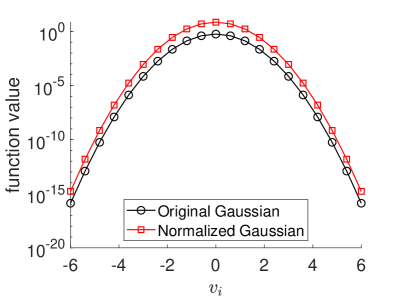
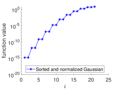
Figure 1: Discretized Gaussian, its normalization and sorted notation in Example 2.6.

Example 2.7.

The second example is for the case where some components of $\boldsymbol{f}^{n+1}$ are zero. We assume a uniform discretization on $[0,1]$ with $\Delta v_{i}=1/N$ for $i=1,\dots,N$ and choose $\boldsymbol{f}^{n+1}$ to be

$$f_{i}^{n+1}=\left\{\begin{array}[]{ll}0,&i=1,\dots,I_{1},\\ 1,&i=I_{1}+1,\dots,N-I_{1},\\ 2,&i=N-I_{1}+1,\dots,N.\end{array}\right.$$

If $I_{1}/N$ is a constant, the vector $\boldsymbol{f}^{n+1}$ approximates a piecewise constant function. In this case, Theorem 2.5 holds by choosing $C_{1}=I_{1}/N$ and $C_{f}$ to be any positive number in $(0,1]$. The blue lines in Fig. 2 show the situation where $C_{1}=1/3$. However, if $I_{1}/N$ decreases to zero as $N$ increases, e.g. $I_{1}\equiv 1$ for all $N$, such a constant $C_{1}$ cannot be found. This situation violates the condition of Theorem 2.5, which is illustrated as the red lines in Fig. 2.

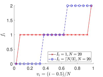
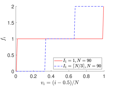
Figure 2: Illustration of Example 2.7 where $f_{i}^{n+1}$ can only be chosen as $0$, $1$ or $2$.

In general, the above theorems suggest that such entropy fix can be safely used without sacrificing the numerical accuracy. Moreover, for a numerical scheme with sufficient accuracy, the violation of the entropy inequality will not always happen, meaning that the entropy fix may be needed only at a few time steps, resulting in even less significant impact on the numerical accuracy.

Remark 2.8.

The above results can be easily generalized to the cases where the equilibrium is not a constant. Assume that $\boldsymbol{\mathcal{M}}=(\mathcal{M}_{1},\cdots,\mathcal{M}_{N})^{T}\in\mathbb{R}_{N}^{+}$ is the equilibrium state of Eq. 1, and the entropy functional (in this case, it is the relative entropy) is defined by

$$\eta[\boldsymbol{f}]=\sum_{i=1}^{N}f_{i}\log\frac{f_{i}}{\mathcal{M}_{i}}\Delta v_{i}.$$

We can let $g_{i}=f_{i}/\mathcal{M}_{i}$ and $\Delta w_{i}=\mathcal{M}_{i}\Delta v_{i}$, so that $\eta[\boldsymbol{f}]$ can be rewritten as

$$\eta[\boldsymbol{f}]=\sum_{i=1}^{N}g_{i}\log g_{i}\Delta w_{i},$$

which fits the entropy formulas in the theorems again. In this case, the entropy fix Eq. 4 applied to $\boldsymbol{g}^{n+1}$ is equivalent to the following fix applied to $\boldsymbol{f}^{n+1}$:

(10) $$\hat{\boldsymbol{f}}^{n+1}=\boldsymbol{f}^{n+1}+\beta_{p}(\boldsymbol{\mathcal{M}}-\boldsymbol{f}^{n+1}).$$

By this transformation, our approach can also be applied to the linear Fokker-Planck equation. Please see the numerical section for more details.

3 Theoretical proofs of the error estimates

This section provides all the details of the proofs of the four theorems. Instead of proving these theorems in the order they are presented, below we will first provide the proof of Theorem 2.3, which can provide necessary tools needed in the proof of Theorem 2.2.

3.1 Proof of Theorem 2.3

Before proving the theorem, the relationship between entropy function and $L^{2}$ norm will be demonstrated by several lemmas. Among them, we will first estimate the entropy function $\eta(\boldsymbol{f})$ and its $L^{2}$ norm $\|\boldsymbol{f}\|_{2}$ in the following lemma.

Lemma 3.1.

For $\boldsymbol{f}\in\mathbb{R}_{+}^{N}$ and $\|\boldsymbol{f}\|_{1}=V$,

$$\frac{1}{2\|\boldsymbol{f}\|_{\infty}}\|\boldsymbol{f}-\boldsymbol{1}\|_{2}^{2}\leq\eta(\boldsymbol{f})\leq\|\boldsymbol{f}-\boldsymbol{1}\|_{2}^{2}.$$

Proof 3.2.

On one hand, for $x\geq 0$,

$$x\log x-(x-1)\leq x(x-1)-(x-1)=(x-1)^{2},$$

where the inequality above uses $\log x\leq x-1$. On the other hand, by Taylor’s theorem,

$$x\log x=(x-1)+\int_{1}^{x}\frac{1}{t}(x-t)\mathrm{d}t.$$

For $0\leq x\leq\|\boldsymbol{f}\|_{\infty}$, the integral satisfies

$$\int_{1}^{x}\frac{1}{t}(x-t)\mathrm{d}t\geq\int_{1}^{x}\frac{1}{\max(x,1)}(x-t)\mathrm{d}t\geq\int_{1}^{x}\frac{1}{\|\boldsymbol{f}\|_{\infty}}(x-t)\mathrm{d}t=\frac{(x-1)^{2}}{2\|\boldsymbol{f}\|_{\infty}}.$$

Therefore,

$$(x-1)+\frac{(x-1)^{2}}{2\|\boldsymbol{f}\|_{\infty}}\leq x\log x\leq(x-1)+(x-1)^{2}.$$

The lemma can be proved by taking $x=f_{i}$ in the above inequality and summing up all $1\leq i\leq N$.

A straightforward corollary of the above lemma is given as follows.

Lemma 3.3.

For $\boldsymbol{f}^{(1)}\in\mathbb{R}_{+}^{N}$ and $\boldsymbol{f}^{(2)}\in\mathbb{R}_{+}^{N}$ with $\|\boldsymbol{f}^{(1)}\|_{1}=\|\boldsymbol{f}^{(2)}\|_{1}=V$, if $\eta(\boldsymbol{f}^{(1)})\leq\eta(\boldsymbol{f}^{(2)})$, then it holds that

$$\|\boldsymbol{f}^{(1)}-\boldsymbol{1}\|_{2}^{2}\leq 2\|\boldsymbol{f}^{(1)}\|_{\infty}\|\boldsymbol{f}^{(2)}-\boldsymbol{1}\|_{2}^{2}.$$

After showing the equivalence between entropy function and 2-norm, we will proceed to discuss the relationship between $\eta(\boldsymbol{f}^{(1)})-\eta(\boldsymbol{f}^{(2)})$ and $\|\boldsymbol{f}^{(1)}-\boldsymbol{f}^{(2)}\|_{2}$ for any two vectors $\boldsymbol{f}^{(1)}$ and $\boldsymbol{f}^{(2)}$. By the definition of $\eta(\cdot)$, we are inspired to study the estimation of $h(x)-h(y)$. The result is presented in the following lemma.

Lemma 3.4.

Given $0<C_{0}\leq 1$, $y\geq 0$ and $x\geq C_{0}$, if $y\geq C_{0}$ or $h(x)>h(y)$, then

(11) $$\left|h(x)-h(y)\right|\leq\max\left(2,2|\log(C_{0})|\right)\left|x-y\right|\left(\left|x-1\right|+\left|y-1\right|\right).$$

Proof 3.5.

If $x=y$, it is obvious that the lemma is correct. It remains to prove the lemma when $x\neq y$.

By the mean value theorem,

(12) $$h(x)-h(y)=\log(\xi)(x-y),$$

where $\xi$ is between $x$ and $y$. If $\log(\xi)\geq 0$, it holds that $\xi\geq 1$ and

$$|\log(\xi)|=\log(\xi)\leq\xi-1\leq\max(x-1,y-1)\leq|x-1|+|y-1|.$$

Therefore, if $\log(\xi)\geq 0$, Eq. 12 becomes

(13) $$|h(x)-h(y)|\leq|x-y|\left(|x-1|+|y-1|\right).$$

Next we assume $h(x)>h(y)$. If $h(x)>h(y)$ and $x>y$, Eq. 12 implies $\log(\xi)>0$, which gives Eq. 13. If $h(x)>h(y)$ and $x<y$, Eq. 12 implies $\log(\xi)<0$ and $\xi\leq 1$. In this case, $y>x\geq C_{0}$, which implies $\xi\geq C_{0}$ and $\log(\xi)\geq\log(C_{0})$. Therefore, Eq. 12 becomes

(14) $$|h(x)-h(y)|=-\log(\xi)|x-y|\leq-\log(C_{0})|x-y|=|\log(C_{0})||x-y|.$$

On the other hand, by the mean value theorem,

$$-\log(\xi)=\log(1)-\log(\xi)=\frac{1}{\xi_{2}}(1-\xi)\leq\frac{1}{C_{0}}\left(|x-1|+|y-1|\right),$$

where $\xi_{2}\in[\xi,1]\subset[C_{0},1]$. The above results can be summarized into the following estimation:

(15) $$|h(x)-h(y)|\leq|x-y|\min\left(|\log(C_{0})|,\frac{1}{C_{0}}\left(|x-1|+|y-1|\right)\right).$$

If we further assume $x\geq 1/2$ and $y\geq 1/2$, then Eq. 15 is satisfied with $C_{0}=1/2$, which becomes

$$|h(x)-h(y)|\leq|x-y|\min\left(\log 2,2\left(|x-1|+|y-1|\right)\right)\leq 2|x-y|\left(|x-1|+|y-1|\right).$$

Otherwise, if $x<1/2$ or $y<1/2$, we have $2(|x-1|+|y-1|)\geq 1$. Therefore,

$$\min\left(|\log(C_{0})|,\frac{1}{C_{0}}\left(|x-1|+|y-1|\right)\right)\leq|\log(C_{0})|\leq 2|\log(C_{0})|\left(|x-1|+|y-1|\right).$$

Combining the two results above yields the inequality (11) when $h(x)>h(y)$.

It remains only to consider the case $h(x)\leq h(y)$ and $y\geq C_{0}$. If $x<y$, Eq. 12 implies $\log(\xi)\geq 0$, which gives the result of Eq. 13. Otherwise, $x>y$ implies $\log(\xi)\leq 0$. Since $x\geq C_{0}$ and $y\geq C_{0}$, it holds that $\xi\geq C_{0}$, and therefore $0\geq\log(\xi)\geq\log(C_{0})$, which also yields Eq. 15. The rest of the proof is the same as the previous case.

With the help of the above lemma, we could give an upper bound of the difference of entropy functions $\eta(\boldsymbol{f}^{(1)})-\eta(\boldsymbol{f}^{(2)})$ in the following lemma.

Lemma 3.6.

For $\boldsymbol{f}^{(1)}=(f^{(1)}_{1},\ldots,f^{(1)}_{N})\in\mathbb{R}_{+}^{N}$ and $\boldsymbol{f}^{(2)}=(f^{(2)}_{1},\ldots,f^{(2)}_{N})\in\mathbb{R}_{+}^{N}$ with $\|\boldsymbol{f}^{(1)}\|_{1}=\|\boldsymbol{f}^{(2)}\|_{1}=V$, given $0<C_{0}\leq 1$, if $f^{(1)}_{i}\geq C_{0}$ for all $1\leq i\leq N$ and $\boldsymbol{f}^{(2)}$ satisfies either of the following conditions:

1. $f^{(2)}_{i}\geq C_{0}$ for all $1\leq i\leq N$;

2. $\eta(\boldsymbol{f}^{(2)})<\eta(\boldsymbol{f}^{(1)})$;

then it holds that

$$|\eta(\boldsymbol{f}^{(1)})-\eta(\boldsymbol{f}^{(2)})|\leq\max\left(2,2|\log(C_{0})|\right)\|\boldsymbol{f}^{(1)}-\boldsymbol{f}^{(2)}\|_{2}\left(\|\boldsymbol{f}^{(1)}-\boldsymbol{1}\|_{2}+\|\boldsymbol{f}^{(2)}-\boldsymbol{1}\|_{2}\right).$$

Proof 3.7.

For simplicity, we use $M$ to denote the constant $\max\left(2,2|\log(C_{0})|\right)$ in this proof. In the first case $f^{(2)}_{i}\geq C_{0}>0$ for all $1\leq i\leq N$, we can plug $x=f^{(1)}_{i}$ and $y=f^{(2)}_{i}$ in Lemma 3.4 and sum over all $1\leq i\leq N$. By using $\|\boldsymbol{f}^{(1)}\|_{1}=\|\boldsymbol{f}^{(2)}\|_{1}$, we can obtain that

$$|\eta(\boldsymbol{f}^{(1)})-\eta(\boldsymbol{f}^{(2)})|\leq M\sum_{i=1}^{N}\left(|(f_{i}^{(1)}-1)(f_{i}^{(1)}-f_{i}^{(2)})|+|(f_{i}^{(2)}-1)(f_{i}^{(1)}-f_{i}^{(2)})|\right)\Delta v_{i}.$$

The lemma can be proven by the Cauchy-Schwarz inequality.

In the second case $\eta(\boldsymbol{f}^{(2)})<\eta(\boldsymbol{f}^{(1)})$, we have

$$\eta(\boldsymbol{f}^{(1)})-\eta(\boldsymbol{f}^{(2)})$$

$$={} \sum_{h(f_{i}^{(1)})\leq h(f_{i}^{(2)})}\left(h(f_{i}^{(1)})-h(f_{i}^{(2)})\right)\Delta v_{i}+\sum_{h(f_{i}^{(1)})>h(f_{i}^{(2)})}\left(h(f_{i}^{(1)})-h(f_{i}^{(2)})\right)\Delta v_{i}$$

$$\leq{} \sum_{h(f_{i}^{(1)})>h(f_{i}^{(2)})}\left(h(f_{i}^{(1)})-h(f_{i}^{(2)})\right)\Delta v_{i}$$

$$\leq{} M\sum_{h(f_{i}^{(1)})>h(f_{i}^{(2)})}\left(|(f_{i}^{(1)}-1)(f_{i}^{(1)}-f_{i}^{(2)})|+|(f_{i}^{(2)}-1)(f_{i}^{(1)}-f_{i}^{(2)})|\right)\Delta v_{i},$$

where the last inequality is again the result of Lemma 3.4. The lemma naturally follows by extending the range of summation of $i$ to $1,\dots,N$ and applying the Cauchy-Schwarz inequality.

In the proof of case 2, we applied Lemma 3.4 only to $f_{i}^{(1)}$ and $f_{i}^{(2)}$ with $h(f_{i}^{(1)})>h(f_{i}^{(2)})$. This allows us to relax the condition “$f^{(1)}_{i}\geq C_{0}$ for all $1\leq i\leq N$” in the case $\eta(\boldsymbol{f}^{(1)})>\eta(\boldsymbol{f}^{(2)})$. In fact, we need $f^{(1)}_{i}>C_{0}$ only for the components that require Lemma 3.4. We write this result in the following corollary:

Corollary 3.8.

For $\boldsymbol{f}^{(1)}=(f^{(1)}_{1},\dots,f^{(1)}_{N})\in\mathbb{R}_{+}^{N}$ and $\boldsymbol{f}^{(2)}=(f^{(2)}_{1},\dots,f^{(2)}_{N})\in\mathbb{R}_{+}^{N}$ with $\|\boldsymbol{f}^{(1)}\|_{1}=\|\boldsymbol{f}^{(2)}\|_{1}=V$, we assume $\eta(\boldsymbol{f}^{(1)})>\eta(\boldsymbol{f}^{(2)})$. If there exists $0<C_{0}<1$ such that for any $i=1,\dots,N$, either $f^{(1)}_{i}\geq C_{0}$ or $h(f_{i}^{(1)})\leq h(f_{i}^{(2)})$ is satisfied, then it holds that

$$|\eta(\boldsymbol{f}^{(1)})-\eta(\boldsymbol{f}^{(2)})|\leq\max\left(2,2|\log(C_{0})|\right)\|\boldsymbol{f}^{(1)}-\boldsymbol{f}^{(2)}\|_{2}\left(\|\boldsymbol{f}^{(1)}-\boldsymbol{1}\|_{2}+\|\boldsymbol{f}^{(2)}-\boldsymbol{1}\|_{2}\right).$$

We are now ready to prove Theorem 2.3.

Proof 3.9 (Proof of Theorem 2.3).

The convexity of $\eta(\cdot)$ implies

$$\eta(\boldsymbol{f}^{n+1}+\beta(\boldsymbol{1}-\boldsymbol{f}^{n+1}))\leq\beta\eta(\boldsymbol{1})+(1-\beta)\eta(\boldsymbol{f}^{n+1}).$$

By Eq. 8 with $\eta(\boldsymbol{1})=0$, the above inequality is equivalent as

(16) $$\beta\leq\frac{\eta(\boldsymbol{f}^{n+1})-\eta(\boldsymbol{f}(t_{n+1}))}{\eta(\boldsymbol{f}^{n+1})}.$$

The numerator in Eq. 16 can be estimated by

$$\eta(\boldsymbol{f}^{n+1})-\eta(\boldsymbol{f}(t_{n+1}))$$

$$\leq{} M\|\boldsymbol{f}^{n+1}-\boldsymbol{f}(t_{n+1})\|_{2}\left(\|\boldsymbol{f}^{n+1}-\boldsymbol{1}\|_{2}+\|\boldsymbol{f}(t_{n+1})-\boldsymbol{1}\|_{2}\right)$$ (Lemma 3.6)

$$\leq{} M\|\boldsymbol{f}^{n+1}-\boldsymbol{f}(t_{n+1})\|_{2}\left(1+\sqrt{\|\boldsymbol{f}(t_{n+1})\|_{\infty}}\right)\|\boldsymbol{f}^{n+1}-\boldsymbol{1}\|_{2},$$ (Lemma 3.3)

where $M=\max(2,2|\log(C_{0})|)$. On the other hand, according to Lemma 3.1, the denominator in Eq. 16 satisfies

$$\eta(\boldsymbol{f}^{n+1})\geq\frac{1}{2\|\boldsymbol{f}^{n+1}\|_{\infty}}\|\boldsymbol{f}^{n+1}-\boldsymbol{1}\|_{2}^{2}.$$

Therefore,

$$\|\beta(\boldsymbol{1}-\boldsymbol{f}^{n+1})\|_{2}\leq 2M\|\boldsymbol{f}^{n+1}\|_{\infty}(1+\sqrt{\|\boldsymbol{f}(t_{n+1})\|_{\infty}})\|\boldsymbol{f}^{n+1}-\boldsymbol{f}(t_{n+1})\|_{2}.$$

In this case, we would like to give a remark on the practical choice of $\beta_{p}$ in Eq. 5. Instead of solving $\eta(\boldsymbol{f}^{n+1}+\beta_{p}(\boldsymbol{1}-\boldsymbol{f}^{n+1}))=\eta(\boldsymbol{f}^{n})$, we can simply take $\hat{\beta}_{p}=({\eta(\boldsymbol{f}^{n+1})-\eta(\boldsymbol{f}^{n})})/{\eta(\boldsymbol{f}^{n+1})}$, which equals the upper bound in Eq. 16. Note that the convexity of function $\eta(\cdot)$ implies $\eta(\boldsymbol{f}^{n})=(1-\hat{\beta}_{p})\eta(\boldsymbol{f}^{n+1})+\hat{\beta}_{p}\eta(\boldsymbol{1})\geq\eta(\boldsymbol{f}^{n+1}+\hat{\beta}_{p}(\boldsymbol{1}-\boldsymbol{f}^{n+1}))$. Therefore, under the condition of Theorem 2.3, if we change the numerical solution at $(n+1)$th step to $\boldsymbol{f}^{n+1}+\hat{\beta}_{p}(\boldsymbol{1}-\boldsymbol{f}^{n+1})$, it still holds that $\|\hat{\beta}_{p}(\boldsymbol{1}-\boldsymbol{f}^{n+1})\|_{2}\leq M\|\boldsymbol{f}(t_{n+1})-\boldsymbol{f}^{n+1}\|_{2}$.

3.2 Proof of Theorem 2.2

Different from the previous proof, in Theorem 2.2, we allow the solution to have components arbitrarily close to zero, so that Lemma 3.6 cannot be directly applied. To overcome this difficulty, we introduce a regularization term before using Lemma 3.6. The details are given as follows.

Proof 3.10 (Proof of Theorem 2.2).

For simplicity, we let $\varepsilon=\|\boldsymbol{f}^{n+1}-\boldsymbol{f}(t_{n+1})\|_{2}$. To avoid dealing with zero components, we first regularize the numerical solution $\boldsymbol{f}^{n+1}$ by

(17) $$\boldsymbol{f}^{n+1,1}=\boldsymbol{f}^{n+1}+\varepsilon(\boldsymbol{1}-\boldsymbol{f}^{n+1}),$$

after which $f^{n+1,1}_{i}\geq\varepsilon$ for all $i=1,\dots,N$. On the other hand, since $\|\boldsymbol{1}-\boldsymbol{f}^{n+1}\|_{\infty}\leq\max(1,\|\boldsymbol{f}\|_{\infty}-1)\leq\|\boldsymbol{f}\|_{\infty}$, the $L^{2}$ norm of the perturbation introduced by the regularization satisfies

$$\|\varepsilon(\boldsymbol{1}-\boldsymbol{f}^{n+1})\|_{2}\leq\sqrt{V}\|\boldsymbol{f}^{n+1}\|_{\infty}\varepsilon.$$

After perturbation, if $\eta(\boldsymbol{f}^{n+1,1})<\eta(\boldsymbol{f}(t_{n+1}))$, then we have $\beta<\varepsilon$ so that the conclusion of the theorem is drawn. If $\eta(\boldsymbol{f}^{n+1,1})>\eta(\boldsymbol{f}(t_{n+1}))$, we can find $\beta_{2}\in(0,1]$ such that

$$\eta(\boldsymbol{f}^{n+1,1}+\beta_{2}(\boldsymbol{1}-\boldsymbol{f}^{n+1,1}))=\eta(\boldsymbol{f}(t_{n+1})),$$

which is identical to Eq. 8 by replacing $\boldsymbol{f}^{n+1}$ to $\boldsymbol{f}^{n+1,1}$. Therefore, we can set $C_{0}=\varepsilon$ in Theorem 2.3 to obtain

$$\|\beta_{2}(\boldsymbol{1}-\boldsymbol{f}^{n+1,1})\|_{2}\leq M_{1}\|\boldsymbol{f}^{n+1,1}-\boldsymbol{f}(t_{n+1})\|_{2},$$

and by the proof of Theorem 2.3, we know that

$$M_{1} =4\max\left(1,\left|\log\varepsilon\right|\right)\|\boldsymbol{f}^{n+1,1}\|_{\infty}(1+\sqrt{\|\boldsymbol{f}(t_{n+1})\|_{\infty}})$$

$$\leq 4(1+\left|\log\varepsilon\right|)\|\boldsymbol{f}^{n+1}\|_{\infty}(1+\sqrt{\|\boldsymbol{f}(t_{n+1})\|_{\infty}}),$$

since $\|\boldsymbol{f}^{n+1,1}\|_{\infty}\leq\|\boldsymbol{f}^{n+1}\|_{\infty}$.

If we define

(18) $$\hat{\boldsymbol{f}}^{n+1}=\boldsymbol{f}^{n+1,1}+\beta_{2}(\boldsymbol{1}-\boldsymbol{f}^{n+1,1})=\boldsymbol{f}^{n+1}+(\varepsilon+\beta_{2}-\varepsilon\beta_{2})(\boldsymbol{1}-\boldsymbol{f}^{n+1}),$$

then by $\eta(\hat{\boldsymbol{f}}^{n+1})=\eta(\boldsymbol{f}(t_{n+1}))$ we know that $\beta=\varepsilon+\beta_{2}-\varepsilon\beta_{2}$. Thus it holds that

$$\|\beta(\boldsymbol{1}-\boldsymbol{f}^{n+1})\|_{2} =\|\hat{\boldsymbol{f}}^{n+1}-\boldsymbol{f}^{n+1}\|_{2}\leq\|\hat{\boldsymbol{f}}^{n+1}-\boldsymbol{f}^{n+1,1}\|_{2}+\|\boldsymbol{f}^{n+1,1}-\boldsymbol{f}^{n+1}\|_{2}$$

$$\leq M_{1}\|\boldsymbol{f}^{n+1,1}-\boldsymbol{f}(t_{n+1})\|_{2}+\|\boldsymbol{f}^{n+1,1}-\boldsymbol{f}^{n+1}\|_{2}$$

$$\leq M_{1}(\|\boldsymbol{f}^{n+1,1}-\boldsymbol{f}^{n+1}\|_{2}+\varepsilon)+\|\boldsymbol{f}^{n+1,1}-\boldsymbol{f}^{n+1}\|_{2}$$

$$\leq M_{1}(\sqrt{V}\|\boldsymbol{f}^{n+1}\|_{\infty}\varepsilon+\varepsilon)+\sqrt{V}\|\boldsymbol{f}^{n+1}\|_{\infty}\varepsilon\leq M_{2}\varepsilon(|\log\varepsilon|+1),$$

where $M_{2}=8(\sqrt{V}\|\boldsymbol{f}^{n+1}\|_{\infty}+1)\|\boldsymbol{f}^{n+1}\|_{\infty}(1+\sqrt{\|\boldsymbol{f}(t_{n+1})\|_{\infty}})$.

The proof of this theorem follows the two-step procedure, which will also be applied in the proof of Theorem 2.4.

3.3 Proof of Theorem 2.4

To prove Theorem 2.4, we deal with the components with $f_{i}^{n+1}<\frac{2}{3}$ and $f_{i}^{n+1}>\frac{2}{3}$ separately. The difference between these two cases can be seen from the following lemma:

Lemma 3.11.

For $\boldsymbol{f}^{(1)}\in\mathbb{R}_{+}^{N}$ and $\boldsymbol{f}^{(2)}\in\mathbb{R}_{+}^{N}$ with $\|\boldsymbol{f}^{(1)}-\boldsymbol{f}^{(2)}\|_{\infty}\leq\frac{1}{3}$, define

$$\boldsymbol{f}^{(3)}=\boldsymbol{f}^{(1)}+\beta_{1}(\boldsymbol{1}-\boldsymbol{f}^{(1)}),$$

where $\beta_{1}=3\|\boldsymbol{f}^{(1)}-\boldsymbol{f}^{(2)}\|_{\infty}$. If $\|\boldsymbol{f}^{(1)}\|_{1}=V$, then $\boldsymbol{f}^{(3)}$ satisfies following properties:

1. For all $k$ such that $f_{k}^{(1)}<\frac{2}{3}$, it holds that $h(f^{(3)}_{k})\leq h(f^{(2)}_{k})$;

2. For all $k$ such that $f_{k}^{(1)}\geq\frac{2}{3}$, it holds that $f^{(3)}_{k}\geq\frac{2}{3}$;

3. $\|\boldsymbol{f}^{(3)}-\boldsymbol{f}^{(1)}\|_{\infty}\leq 3\|\boldsymbol{f}^{(1)}\|_{\infty}\|\boldsymbol{f}^{(1)}-\boldsymbol{f}^{(2)}\|_{\infty}$.

Proof 3.12.

For those $k$ such that $f_{k}^{(1)}<\frac{2}{3}$, we have $1-f_{k}^{(1)}\geq\frac{1}{3}$. Thus

$$f_{k}^{(3)}-f_{k}^{(1)}=\beta_{1}(1-f_{k}^{(1)})\geq 3|f^{(1)}_{k}-f^{(2)}_{k}|\cdot(1-f_{k}^{(1)})\geq|f^{(1)}_{k}-f^{(2)}_{k}|\geq f^{(2)}_{k}-f^{(1)}_{k},$$

which yields $f_{k}^{(3)}\geq f_{k}^{(2)}$. Since $f_{k}^{(3)}$ is the convex combination of $1$ and $f_{k}^{(1)}$, we have $0\leq f_{k}^{(3)}\leq 1$. Since $h(\cdot)$ is monotonically decreasing on $[0,1]$, we conclude that $h(f^{(3)}_{k})\leq h(f^{(2)}_{k})$.

The second property is obvious since $f_{k}^{(3)}$ lies between $f_{k}^{(1)}$ and $1$.

As for the third property, it should be noted that $\|\boldsymbol{f}^{(1)}\|_{1}=V$ implies $\|\boldsymbol{f}^{(1)}\|_{\infty}\geq 1$. Therefore,

$$\|\boldsymbol{f}^{(3)}-\boldsymbol{f}^{(1)}\|_{\infty} =\beta_{1}\|\boldsymbol{1}-\boldsymbol{f}^{(1)}\|_{\infty}$$

$$\leq\max(1,\|\boldsymbol{f}^{(1)}\|_{\infty}-1)\beta_{1}\leq 3\|\boldsymbol{f}^{(1)}\|_{\infty}\|\boldsymbol{f}^{(1)}-\boldsymbol{f}^{(2)}\|_{\infty}.$$

The first property in Lemma 3.11 shows how we deal with the small components, and this only holds when $\beta_{1}$ is proportional to the difference between $\boldsymbol{f}^{(1)}$ and $\boldsymbol{f}^{(2)}$ measured by the infinity norm, leading to the form of the right-hand side in the conclusion of Theorem 2.4. For the remaining terms, an $O(1)$ lower bound exists, so that the same technique as Theorem 2.3 can be applied. The details of the proof are given below:

Proof 3.13 (Proof of Theorem 2.4).

By Lemma 3.11, we could pick $\beta_{1}=3\|\boldsymbol{f}^{n+1}-\boldsymbol{f}(t_{n+1})\|_{\infty}$ and construct

(19) $$\boldsymbol{f}^{n+1,1}=\boldsymbol{f}^{n+1}+\beta_{1}(\boldsymbol{1}-\boldsymbol{f}^{n+1}),$$

If $\eta(\boldsymbol{f}^{n+1,1})\leq\eta(\boldsymbol{f}(t_{n+1}))$, the proof is already completed. If $\eta(\boldsymbol{f}^{n+1,1})>\eta(\boldsymbol{f}(t_{n+1}))$, we construct $\hat{\boldsymbol{f}}^{n+1}$ as Eq. 18 such that $\eta(\hat{\boldsymbol{f}}^{n+1})=\eta(\boldsymbol{f}(t_{n+1}))$, and thus $\beta=\beta_{1}+\beta_{2}-\beta_{1}\beta_{2}$. According to Lemma 3.11, those components $i$ where $h(f_{i}^{n+1,1})>h(f_{i}(t_{n+1}))$ satisfy $f_{i}^{n+1,1}\geq\frac{2}{3}$. Therefore, Corollary 3.8 could be applied with $C_{0}=\frac{2}{3}$, and we could mimic the proof of Theorem 2.3 with only replacement from Lemma 3.6 to Corollary 3.8 in the proof. As a result, by the conclusion of Theorem 2.3, it holds that

$$\|\beta_{2}(\boldsymbol{1}-\boldsymbol{f}^{n+1,1})\|_{2}\leq M_{1}\|\boldsymbol{f}(t_{n+1})-\boldsymbol{f}^{n+1,1}\|_{2},$$

where $M_{1}=4\max\left(1,|\log(C_{0})|\right)\|\boldsymbol{f}^{n+1,1}\|_{\infty}(1+\sqrt{\|\boldsymbol{f}(t_{n+1})\|_{\infty}})$ taken from the proof of Theorem 2.3. Moreover, $\boldsymbol{f}^{n+1,1}$ in $M_{1}$ could be replaced by $\boldsymbol{f}^{n+1}$ since $\|\boldsymbol{f}^{n+1,1}\|_{\infty}\leq\|\boldsymbol{f}^{n+1}\|_{\infty}$. Then, similar to the second step in the proof of Theorem 2.2, it holds that

$$\|\hat{\boldsymbol{f}}^{n+1}-\boldsymbol{f}^{n+1}\|_{2} \leq\|\hat{\boldsymbol{f}}^{n+1}-\boldsymbol{f}^{n+1,1}\|_{2}+\|\boldsymbol{f}^{n+1,1}-\boldsymbol{f}^{n+1}\|_{2}$$

$$\leq M_{1}\|\boldsymbol{f}(t_{n+1})-\boldsymbol{f}^{n+1,1}\|_{2}+\|\boldsymbol{f}^{n+1,1}-\boldsymbol{f}^{n+1}\|_{2}$$

$$\leq M_{1}\sqrt{V}\|\boldsymbol{f}(t_{n+1})-\boldsymbol{f}^{n+1,1}\|_{\infty}+\sqrt{V}\|\boldsymbol{f}^{n+1,1}-\boldsymbol{f}^{n+1}\|_{\infty}$$

$$\leq M_{1}\sqrt{V}\|\boldsymbol{f}(t_{n+1})-\boldsymbol{f}^{n+1}\|_{\infty}+\sqrt{V}(M_{1}+1)\|\boldsymbol{f}^{n+1,1}-\boldsymbol{f}^{n+1}\|_{\infty}$$

$$\leq\left(M_{1}\sqrt{V}+3\sqrt{V}(M_{1}+1)\|\boldsymbol{f}^{n+1}\|_{\infty}\right)\|\boldsymbol{f}(t_{n+1})-\boldsymbol{f}^{n+1}\|_{\infty},$$

where the last “$\leq$” is the result of Lemma 3.11. This completes the proof since $\|\beta(\boldsymbol{1}-\boldsymbol{f}^{n+1})\|_{2}=\|\hat{\boldsymbol{f}}^{n+1}-\boldsymbol{f}^{n+1}\|_{2}$.

3.4 Proof of Theorem 2.5

In this subsection, we will prove Theorem 2.5. Before that, we would like to introduce two lemmas. Lemma 3.14 comes from optimization, which illustrates the infinity norm of optimal solution could be bounded by the $L^{2}$ norm of it. Based on Lemma 3.14, we make a decomposition of the (relative) entropy function in Eq. 31 and then introduce Lemma 3.21 to estimate the difference of decomposed entropy functions.

As assumed in the theorem, we suppose all the components of $\boldsymbol{f}$ are sorted in the ascending order:

$$f_{1}\leq f_{2}\leq\cdots\leq f_{N}=\|\boldsymbol{f}\|_{\infty}.$$

Note that this does not affect the definition of entropy and the numerical scheme for the entropy fix.

Lemma 3.14.

For any $C_{1},C_{f}\in(0,1]$ and positive integer $N$, let $I_{1}=\min\{I\mid\sum_{i=1}^{I}\Delta v_{i}\geq C_{1}V\}$. If $\boldsymbol{f}\in\mathbb{R}_{+}^{N}$ satisfies

$$f_{i}\leq 1/2\text{ for all }i=1,\ldots,I_{1}\qquad\text{and}\qquad\frac{1}{|\log f_{1}|}\geq\frac{C_{f}}{|\log f_{I_{1}}|},$$

then when $\varepsilon<\frac{1}{2}\sqrt{C_{1}V}$, the solution $\boldsymbol{g}^{*}=(g^{*}_{1},\ldots,g^{*}_{I_{1}})^{T}\in\mathbb{R}^{I_{1}}$ of the following optimization problem

(20) $$\operatorname*{argmin}_{g_{1},\ldots,g_{I_{1}}}\sum_{i=1}^{I_{1}}h(f_{i}+g_{i})\Delta v_{i},\qquad\text{s.t. }\sum_{i=1}^{I_{1}}g_{i}^{2}\Delta v_{i}\leq\varepsilon^{2},$$

satisfies $0\leq g_{I_{1}}^{*}\leq\cdots\leq g_{1}^{*}\leq(\sqrt{C_{1}V}C_{f})^{-1}\varepsilon$ and $C_{f}\leq g_{I_{1}}^{*}/g_{1}^{*}\leq 1$.

Proof 3.15.

The proof utilizes the Karush–Kuhn–Tucker (KKT) sufficient conditions for optimization problems [11, Chapter 3.5]. It is easy to verify that both the objective function and the constraint are continuously differentiable convex functions with respect to $(g_{1},\ldots,g_{I_{1}})^{T}$. Therefore, if the following conditions hold for $\lambda^{*}\in\mathbb{R}$ and $\boldsymbol{g}^{*}=(g_{1}^{*},\ldots,g_{I_{1}}^{*})^{T}$,

(21) $$\left\{\begin{aligned} &h^{\prime}(f_{i}+g_{i}^{*})+2\lambda^{*}g_{i}^{*}=0,\qquad\forall\ 1\leq i\leq I_{1},\\ &\sum_{i=1}^{I_{1}}(g_{i}^{*})^{2}\Delta v_{i}\leq\varepsilon^{2},\\ &\lambda^{*}\geq 0,\\ &\lambda^{*}(\sum_{i=1}^{I_{1}}(g_{i}^{*})^{2}\Delta v_{i}-\varepsilon^{2})=0,\end{aligned}\right.$$

then $\boldsymbol{g}^{*}$ is the global minimum of the optimization problem.

First, we claim that $\lambda^{*}\neq 0$, so that

(22) $$\sum_{i=1}^{I_{1}}(g_{i}^{*})^{2}\Delta v_{i}=\varepsilon^{2}$$

due to the last equation in Eq. 21. If $\lambda^{*}$ equals $0$, then $h^{\prime}(f_{i}+g_{i}^{*})=0$, which yields $g_{i}^{*}=1-f_{i}\geq\frac{1}{2}$. Therefore,

$$\sum_{i=1}^{I_{1}}(g_{i}^{*})^{2}\Delta v_{i}\geq\frac{\sum_{i=1}^{I_{1}}\Delta v_{i}}{4}\geq\frac{C_{1}V}{4}>\varepsilon^{2},$$

which contradicts with the second inequality in Eq. 21.

Now we would like to establish the existence and uniqueness of the solution. We first focus on the first equation in Eq. 21. For any $1\leq i\leq I_{1}$ and fixed $\lambda^{*}>0$, there exist one unique $g_{i}^{*}\in(0,1)$ satisfying $h^{\prime}(f_{i}+g_{i}^{*})+2\lambda^{*}g_{i}^{*}=0$. This is because the function $\zeta_{i}(x):=h^{\prime}(f_{i}+x)+2\lambda^{*}x$ is monotonically increasing, and

$$\zeta(0)=\log f_{i}\leq\log(\frac{1}{2})<0,\qquad\zeta(1)\geq 2\lambda^{*}>0.$$

Thus it remains to demonstrate that $\lambda^{*}$ is unique. Inspired by the first equation in Eq. 21, we define

$$\sigma(x)=-\frac{h^{\prime}(f_{i}+x)}{2x}=-\frac{\log(f_{i}+x)}{2x},\qquad x\in(0,1-f_{i}].$$

Then its inverse function $\sigma_{i}^{-1}(y)$ satisfies

(23) $$y=-\frac{\log(f_{i}+\sigma_{i}^{-1}(y))}{2\sigma_{i}^{-1}(y)}\quad\text{and}\quad\sigma_{i}^{-1}(y)=\frac{W_{0}(2ye^{2yf_{i}})-2yf_{i}}{2y},$$

where $W_{0}(\cdot)$ is the Lambert $W$ function [5] satisfying $W_{0}(x)e^{W_{0}(x)}=x$. For $\sigma_{i}(\cdot)$ and $\sigma_{i}^{-1}(\cdot)$, we have the following properties:

1. $\sigma_{i}(x)$ is monotonically decreasing, so is $\sigma_{i}^{-1}(x)$ (this requires $f_{i}\leq\frac{1}{2}$);

2. $\sigma_{i}(g_{i}^{*})=\lambda^{*}$ and $g_{i}^{*}=\sigma_{i}^{-1}(\lambda^{*})$;

3. $\sigma_{i}^{-1}(0)=1-f_{i}\geq\frac{1}{2}$ and $\sigma_{i}^{-1}(y)\rightarrow 0$ as $y\rightarrow+\infty$.

Here the limit of $\sigma_{i}^{-1}(y)$ at $+\infty$ can be obtained by the inequality (see [8])

$$W_{0}(x)\leq\log(x)-\log(\log(x))+\frac{e}{e-1}\frac{\log(\log(x))}{\log(x)},\qquad\forall x\geq e.$$

Furthermore, if we define

$$\Xi(y)=\sum_{i=1}^{I_{1}}[\sigma_{i}^{-1}(y)]^{2}\Delta v_{i},\qquad y\in[0,+\infty),$$

then by the three properties of $\sigma_{i}$, we have

1. $\Xi(y)$ is a decreasing function since each $\sigma_{i}^{-1}(y)$ is monotonically decreasing;

2. $\Xi(\lambda^{*})=\varepsilon^{2}$ according to Eq. 22;

3. $\Xi(0)\geq\frac{1}{4}\sum_{i=1}^{I_{1}}\Delta v_{i}>\varepsilon^{2}$, and $\Xi(y)\rightarrow 0$ as $y\rightarrow+\infty$.

These properties show the existence and uniqueness of $\lambda^{*}$.

Next, we will show $g_{I_{1}}^{*}\leq\cdots\leq g_{1}^{*}$. For any $1\leq i\leq j\leq I_{1}$, $f_{i}\leq f_{j}$ implies

$$\sigma_{j}(g_{j}^{*})=\lambda^{*}=\sigma_{i}(g_{i}^{*})\geq\sigma_{j}(g_{i}^{*}).$$

Using the fact that $\sigma_{j}(\cdot)$ is decreasing, we see that $g_{j}^{*}\leq g_{i}^{*}$. To get the bound of $g_{1}^{*}$, we need the following two results:

• By Eq. 23, we have

  $$\lim_{y\rightarrow+\infty}\frac{\sigma_{i}^{-1}(y)}{\sigma_{1}^{-1}(y)}=\lim_{y\rightarrow+\infty}\frac{\log(f_{i}+\sigma_{i}^{-1}(y))}{\log(f_{1}+\sigma_{1}^{-1}(y))}=\frac{\log(f_{i})}{\log(f_{1})}\geq C_{f};$$

• By straightforward calculation, we have

  $$\frac{\mathrm{d}}{\mathrm{d}y}\left(\frac{\sigma_{i}^{-1}(y)}{\sigma_{1}^{-1}(y)}\right)=\frac{W_{0}(2ye^{2yf_{1}})-W_{0}(2ye^{2yf_{i}})}{y(1+W_{0}(2ye^{2yf_{1}}))(1+W_{0}(2ye^{2yf_{i}}))}\frac{\sigma_{i}^{-1}(y)}{\sigma_{1}^{-1}(y)}\leq 0.$$

These results indicate that

$$\frac{g_{i}^{*}}{g_{1}^{*}}=\frac{\sigma_{i}^{-1}(\lambda^{*})}{\sigma_{1}^{-1}(\lambda^{*})}\geq C_{f},$$

and thus

$$g_{1}^{*}=\varepsilon\left(\sum_{i=1}^{I_{1}}\frac{(g_{i}^{*})^{2}}{(g_{1}^{*})^{2}}\Delta v_{i}\right)^{-1/2}\leq\varepsilon\left(\sum_{i=1}^{I_{1}}C_{f}^{2}\Delta v_{i}\right)^{-1/2}\leq\frac{\varepsilon}{\sqrt{C_{1}V}C_{f}}.$$

This completes the proof.

One corollary of the above lemma is the extension to a continuous version, with identical optimal solution $\boldsymbol{g}^{*}$ in the sense of piesewise constant function. For the ease of this extension, we would like to introduce the (partial) sum of first $i$ parameters $\Delta v_{i}$ as

(24) $$S_{0}=0,\qquad S_{i}=\sum_{j=1}^{i}\Delta v_{j},\qquad i=1,\dots,N.$$

Then we have the following lemma.

Corollary 3.16.

Under the condition of Lemma 3.14, if a piesewise constant function defined on $(0,S_{I_{1}}]$ is introduced as

$$f(v)=f_{i},\qquad v\in(S_{i-1},S_{i}],\quad i=1,\dots,I_{1},$$

then the solution $g^{*}(v)\in L^{2}((0,S_{I_{1}}])$ of the following optimization problem

(25) $$\operatorname*{argmin}_{g\in L^{2}((0,S_{I_{1}}])}\int_{0}^{S_{I_{1}}}h(f(v)+g(v))\mathrm{d}v,\qquad\text{s.t. }\|g\|_{2}^{2}:=\int_{0}^{S_{I_{1}}}(g(v))^{2}\mathrm{d}v\leq\varepsilon^{2},$$

is equal to a piecewise constant function a.e. as

$$g^{*}(v)=g^{*}_{i},\qquad v\in(S_{i-1},S_{i}],\quad i=1,\dots,I_{1},$$

where $g^{*}_{i}$ is the component of the optimal solution $\boldsymbol{g}^{*}$ in Lemma 3.14.

Proof 3.17.

To prove the corollary, it suffices to show that for every $i=1,\cdots,I_{1}$, the function $g^{*}(v)$ is a constant on $(S_{i-1},S_{i}]$ except for a set with measure zero, so that the optimization problem Eq. 25 is essentially equivalent to Eq. 20. Suppose that $g^{*}(v)$ is essentially not a constant on $(S_{i-1},S_{i}]$ for some $i$. We define the function $\hat{g}(v)$ by

$$\hat{g}(v)=\left\{\begin{array}[]{ll}\frac{1}{\Delta v_{i}}\int_{S_{i-1}}^{S_{i}}g^{*}(v)\,\mathrm{d}v,&\text{if }v\in(S_{i-1},S_{i}],\\ g^{*}(v),&\text{otherwise}.\end{array}\right.$$

By Hölder’s inequality (on $(S_{i-1},S_{i}]$), it is easy to find $\|\hat{g}\|_{2}^{2}\leq\|g^{*}\|_{2}^{2}\leq\varepsilon^{2}$. Moreover, using Jensen’s inequality on convex function $h(f_{i}+\cdot)$, we obtain

(26) $$\int_{S_{i-1}}^{S_{i}}h(f(v)+\hat{g}(v))\,\mathrm{d}v=\Delta v_{i}h(f_{i}+\hat{g}(v))\leq\int_{S_{i-1}}^{S_{i}}h(f_{i}+g^{*}(v))\,\mathrm{d}v.$$

Note that $g^{*}(\cdot)$ is the optimal solution, implying that the equality must hold for (26). However, since $h(f_{i}+\cdot)$ is strictly convex, the equality holds only when $g^{*}(v)$ is a constant on $(S_{i-1},S_{i}]$, which contradicts our assumption. This completes the proof of the corollary.

Another important corollary of Lemma 3.14 is to pick $\beta_{1}=O(\|\boldsymbol{f}^{n+1}-\boldsymbol{f}(t_{n+1})\|_{2})$ and construct $\boldsymbol{f}^{n+1,1}$ following Eq. 19, such that the entropy of $\boldsymbol{f}^{n+1,1}$ is less than the entropy of $\boldsymbol{f}(t_{n+1})$ in the range of $i\leq I_{1}$.

Corollary 3.18.

Let $\varepsilon:=\|\boldsymbol{f}^{n+1}-\boldsymbol{f}(t_{n+1})\|_{2}$. Suppose $\boldsymbol{f}^{n+1}$ satisfies the condition of Lemma 3.14 and $\varepsilon<\frac{\sqrt{C_{1}V}C_{f}}{2}$. Let $\beta_{1}=\frac{2\varepsilon}{\sqrt{C_{1}V}C_{f}}$ and

(27) $$\boldsymbol{f}^{n+1,1}=\boldsymbol{f}^{n+1}+\beta_{1}(\boldsymbol{1}-\boldsymbol{f}^{n+1}).$$

Then $\boldsymbol{f}^{n+1,1}$ satisfies

(28) $$\sum_{i=1}^{I_{1}}h(f^{n+1,1}_{i})\Delta v_{i}\leq\sum_{i=1}^{I_{1}}h(f_{i}(t_{n+1}))\Delta v_{i}.$$

Proof 3.19.

Let $g_{1}^{*},\ldots,g_{I_{1}}^{*}$ be the solution of the optimization problem Eq. 20. Since

$$\sum_{i=1}^{I_{1}}(f_{i}^{n+1}-f_{i}(t_{n+1}))^{2}\Delta v_{i}\leq\|\boldsymbol{f}^{n+1}-\boldsymbol{f}(t_{n+1})\|_{2}^{2}=\varepsilon^{2},$$

it holds that

$$\sum_{i=1}^{I_{1}}h(f^{n+1}_{i}+g_{i}^{*})\Delta v_{i}\leq\sum_{i=1}^{I_{1}}h(f_{i}(t_{n+1}))\Delta v_{i}.$$

To prove Eq. 28, it suffices to show

(29) $$\sum_{i=1}^{I_{1}}h(f^{n+1,1}_{i})\Delta v_{i}\leq\sum_{i=1}^{I_{1}}h(f^{n+1}_{i}+g_{i}^{*})\Delta v_{i}.$$

By the conclusion of Lemma 3.14,

$$f_{i}^{n+1,1}=f_{i}^{n+1}+\beta_{1}(1-f_{i}^{n+1})\geq f_{i}^{n+1}+\frac{\beta_{1}}{2}=f_{i}^{n+1}+\frac{\varepsilon}{\sqrt{C_{1}V}C_{f}}\geq f_{i}^{n+1}+g_{i}^{*},$$

for all $1\leq i\leq I_{1}$. Noticing that $\beta_{1}<1$ by the constraint $\varepsilon<\frac{\sqrt{C_{1}V}C_{f}}{2}$, we obtain $f_{i}^{n+1,1}<1$. Hence, the monotonicity of $h(\cdot)$ yields

$$h(f_{i}^{n+1,1})\leq h(f_{i}^{n+1}+g_{i}^{*}),\qquad\forall i=1,\ldots,I_{1}.$$

Multiplying $\Delta v_{i}$ and summing up the above inequalities for $i$ yields Eq. 29.

By Corollary 3.18, we have performed our first step that reduce the entropy of the smallest part of $\boldsymbol{f}^{n+1}$ (from $f_{1}^{n+1}$ to $f_{I_{1}}^{n+1}$) below the entropy of the exact solution in the same section. If the smallest component beyond this section $f_{I_{1}+1}^{n+1}$ already has the magnitude $O(1)$, for instance, $f_{I_{1}+1}^{n+1}\geq\frac{1}{2}$, then the remaining part can be processed using the same technique as in Theorem 2.2 and Theorem 2.4. Therefore, below we will only focus on the case where $f_{I_{1}+1}^{n+1}<1/2$, and this inspires us to further decompose the remaining components into two parts by introducing $I_{2}$ such that

(30) $$f_{I_{2}}^{n+1}\leq\frac{1}{2},\qquad f_{I_{2}+1}^{n+1}>\frac{1}{2}.$$

Then we will have $\eta(\boldsymbol{f})-V=H_{1}(\boldsymbol{f})+H_{2}(\boldsymbol{f})+H_{3}(\boldsymbol{f})$ for any $\boldsymbol{f}\in\mathbb{R}_{+}^{N}$, where

(31) $$H_{1}(\boldsymbol{f})=\sum_{i=1}^{I_{1}}h(f_{i})\Delta v_{i},\quad H_{2}(\boldsymbol{f})=\sum_{i=I_{1}+1}^{I_{2}}h(f_{i})\Delta v_{i},\quad H_{3}(\boldsymbol{f})=\sum_{i=I_{2}+1}^{N}h(f_{i})\Delta v_{i}.$$

Note that this decomposition also includes the case $f_{I_{1}+1}^{n+1}\geq\frac{1}{2}$, for which we can choose $I_{2}=I_{1}$, so that $H_{2}(\boldsymbol{f}^{n+1})=0$.

Lemma 3.21 will show some properties of above decomposition. Before that, a quotient $F(x,y,C)$, which will be used in the proof of Lemma 3.21, is introduced as

(32) $$F(x,y,C)=\frac{h(x+y)-h(x+Cy)}{h(x)-h(x+y)},$$

where $0\leq x\leq 1/2$, $C>1$ and $0\leq y\leq 1/(2C)$. It is easy to find $F(x,y,C)\geq 0$ in its domain of definition. Furthermore, the following lemma gives the positive lower bound of $F(x,y,C)$ for fixed $C$, where the proof utilizes the (partial) derivatives of $F(x,y,C)$ and its detail is left in Appendix A.

Lemma 3.20.

For any $C_{1}\in(0,1]$, there exists $C_{2}>1$ depending on $C_{1}$, such that $F(x,y,C_{2})$ given in Eq. 32 satisfies

$$F(x,y,C_{2})\geq\frac{1}{C_{1}},\qquad\forall 0\leq x\leq 1/2,\ 0\leq y\leq\frac{1}{2C_{2}}.$$

Lemma 3.21.

Under the condition of Corollary 3.18 and the decomposition of Eq. 31, the following properties are satisfied:

1. $H_{2}(\boldsymbol{f}^{n+1,1})-H_{2}(\boldsymbol{f}(t_{n+1}))\leq\frac{1}{C_{1}}(H_{1}(\boldsymbol{f}^{n+1})-H_{1}(\boldsymbol{f}^{n+1,1}))$;

2. There exists a constant $M_{1}>1$ depending on $C_{1}$ such that when $\varepsilon\leq\frac{\sqrt{C_{1}V}C_{f}}{2M_{1}}$, the vector

   (33) $$\boldsymbol{f}^{n+1,2}=\boldsymbol{f}^{n+1,1}+M_{1}\beta_{1}(\boldsymbol{1}-\boldsymbol{f}^{n+1,1})$$

   satisfies $H_{1}(\boldsymbol{f}^{n+1,1})-H_{1}(\boldsymbol{f}^{n+1,2})\geq\frac{1}{C_{1}}(H_{1}(\boldsymbol{f}^{n+1})-H_{1}(\boldsymbol{f}^{n+1,1}))$.

Proof 3.22.

To prove the first statement, we use the convexity of $H_{2}(\cdot)$ to obtain

(34) $$H_{2}(\boldsymbol{f}^{n+1,1})=H_{2}(\boldsymbol{f}^{n+1}+\beta_{1}(\boldsymbol{1}-\boldsymbol{f}^{n+1}))\leq\max(H_{2}(\boldsymbol{f}^{n+1}),H_{2}(\boldsymbol{1}))=H_{2}(\boldsymbol{f}^{n+1}).$$

Therefore,

(35) $$H_{2}(\boldsymbol{f}^{n+1,1})-H_{2}(\boldsymbol{f}(t_{n+1}))$$

$$={} H_{2}(\boldsymbol{f}^{n+1,1})-H_{2}(\boldsymbol{f}^{n+1})+H_{2}(\boldsymbol{f}^{n+1})-H_{2}(\boldsymbol{f}(t_{n+1}))$$

$$\leq{} H_{2}(\boldsymbol{f}^{n+1})-H_{2}(\boldsymbol{f}(t_{n+1}))\leq H_{2}(\boldsymbol{f}^{n+1})-H_{2}(\boldsymbol{f}^{n+1}+\boldsymbol{g}^{**}),$$

where $\boldsymbol{g}^{**}=(g^{**}_{1},\ldots,g^{**}_{N})^{T}\in\mathbb{R}^{N}$ is the solution of following minimization problem:

$$\operatorname*{argmin}_{\|\boldsymbol{g}\|_{2}\leq\varepsilon}H_{2}(\boldsymbol{f}^{n+1}+\boldsymbol{g}).$$

The existence of $\boldsymbol{g}^{**}$ is because $H_{2}(\boldsymbol{f}^{n+1}+\boldsymbol{g})$ is a continuous function (w.r.t. $\boldsymbol{g}$) defined on a closed set and the constrain $\|\boldsymbol{g}\|_{2}\leq\varepsilon$ also gives a closed set for $\boldsymbol{g}$. The solution $\boldsymbol{g}^{**}$ satisfies that $g^{**}_{i}\geq 0$ for all $I_{1}<i\leq I_{2}$, since replacing any negative component of $\boldsymbol{g}$ by zero will lead to a smaller value for the objective function.

For any $i=I_{1}+1,\ldots,I_{2}$ and $j=1,\ldots,I_{1}$, the convexity of $h(\cdot)$ implies

(36) $$h(f_{i}^{n+1})-h(f_{i}^{n+1}+g^{**}_{i})\leq h(f^{n+1}_{j})-h(f^{n+1}_{j}+g^{**}_{i}).$$

To extend the above inequality to functions defined on $\mathbb{R}_{+}$ with support in $[0,V]$, which is convenient for our proof in the following step, we would like to follow the notation in Eq. 24 and represent $\boldsymbol{f}^{n+1}$ and $\boldsymbol{g}^{**}$ by piesewise constant functions $f^{n+1}(v)$ and $g^{**}(v)$ respectively as

$$f^{n+1}(v)=f^{n+1}_{i},\qquad g^{**}(v)=g^{**}_{i},\qquad v\in(S_{i-1},S_{i}],\ i=1,\dots,I_{2},$$

and both $f^{n+1}(v)$ and $g^{**}(v)$ equal zero if $v>S_{I_{2}}$. Using the functions $f^{n+1}(v)$ and $g^{**}(v)$, the inequality Eq. 36 is equivalent to: for any $w\in(S_{I_{1}},S_{I_{2}})$ and $v\in(S_{0},S_{I_{1}})$,

$$h(f^{n+1}(w))-h(f^{n+1}(w)+g^{**}(w))\leq h(f^{n+1}(v))-h(f^{n+1}(v)+g^{**}(w)).$$

Since $g^{**}(w)=0$ for $w\geq S_{I_{2}}$, the above inequality actually holds for any $w\in(S_{I_{1}},+\infty)$. Therefore, we choose $w=v+kS_{I_{1}}$ with $k\geq 1$ to obtain

(37) $$H_{2}(\boldsymbol{f}^{n+1})-H_{2}(\boldsymbol{f}^{n+1}+\boldsymbol{g}^{**})$$

$$={} \sum_{i=I_{1}+1}^{I_{2}}\left(h(f^{n+1}_{i})-h(f^{n+1}_{i}+g^{**}_{i})\right)\Delta v_{i}$$

$$={} \int_{S_{I_{1}}}^{S_{I_{2}}}\left(h(f^{n+1}(v))-h(f^{n+1}(v)+g^{**}(v))\right)\mathrm{d}v$$

$$={} \sum_{k=1}^{\left\lceil\frac{S_{I_{2}}-S_{I_{1}}}{S_{I_{1}}}\right\rceil}\int_{0}^{S_{I_{1}}}\left(h(f^{n+1}(v+kS_{I_{1}}))-h(f^{n+1}(v+kS_{I_{1}})+g^{**}(v+kS_{I_{1}}))\right)\mathrm{d}v$$

$$\leq{} \sum_{k=1}^{\left\lceil\frac{S_{I_{2}}-S_{I_{1}}}{S_{I_{1}}}\right\rceil}\int_{0}^{S_{I_{1}}}\left(h(f^{n+1}(v))-h(f^{n+1}(v)+g^{**}(v+kS_{I_{1}}))\right)\mathrm{d}v.$$

Since $\|g^{**}\|_{2}^{2}\leq\|\boldsymbol{g}^{**}\|_{2}^{2}\leq\varepsilon^{2}$, for any $1\leq k\leq\lceil\frac{S_{I_{2}}-S_{I_{1}}}{S_{I_{1}}}\rceil$, we have

(38) $$\int_{0}^{S_{I_{1}}}h(f^{n+1}(v)+g^{**}(v+kS_{I_{1}}))\mathrm{d}v$$

$$\geq{} \int_{0}^{S_{I_{1}}}h(f^{n+1}(v)+g^{*}(v))\mathrm{d}v$$

$$={} \sum_{j=1}^{I_{1}}h(f^{n+1}_{j}+g_{j}^{*})\Delta v_{j}\geq\sum_{j=1}^{I_{1}}h(f^{n+1,1}_{j})\Delta v_{j},$$

where $g^{*}(v)$ and $g_{i}^{*}$ stand for the solutions of the optimization problem Eq. 25 and Eq. 20, respectively; the equality is the conclusion of Corollary 3.16, and the last “$\geq$” comes from the inequality Eq. 29. Inserting Eq. 38 into Eq. 37 yields

(39) $$H_{2}(\boldsymbol{f}^{n+1})-H_{2}(\boldsymbol{f}^{n+1}+\boldsymbol{g}^{**}) \leq\sum_{k=1}^{\lceil\frac{S_{I_{2}}-S_{I_{1}}}{S_{I_{1}}}\rceil}\sum_{j=1}^{I_{1}}\left(h(f^{n+1}_{j})-h(f^{n+1,1}_{j})\right)\Delta v_{j}$$

$$\leq\frac{V}{S_{I_{1}}}(H_{1}(\boldsymbol{f}^{n+1})-H_{1}(\boldsymbol{f}^{n+1,1})).$$

Since the definition of $I_{1}$ implies $S_{I_{1}}\geq C_{1}V$, concatenating Eq. 35 and (39) proves the first statement.

The second statement will be proved componentwisely. We set $M_{1}=2C_{2}$, where $C_{2}$ is determined by Lemma 3.20 with $C_{1}$ being chosen as the constant $C_{1}$ appearing in the first statement. Then, for any $1\leq i\leq I_{1}$, it holds that

$$f_{i}^{n+1,1}=f_{i}^{n+1}+\beta_{1}(1-f^{n+1}_{i})\leq f_{i}^{n+1}+\beta_{1}.$$

Moreover, when $\varepsilon\leq\frac{\sqrt{C_{1}V}C_{f}}{2M_{1}}$, it could be found that $\beta_{1}\leq 1/M_{1}$ and

$$f_{i}^{n+1,2} =f_{i}^{n+1}+(\beta_{1}+M_{1}\beta_{1}-M_{1}\beta_{1}^{2})(1-f^{n+1}_{i})$$

$$\geq f_{i}^{n+1}+M_{1}\beta_{1}(1-f^{n+1}_{i})\geq f_{i}^{n+1}+C_{2}\beta_{1},$$

where we have used $f_{i}^{n+1}\leq\frac{1}{2}$ and $M_{1}=2C_{2}$. Therefore, the monotonicity of $h(\cdot)$ in the interval of $[0,1]$ implies

$$\frac{h(f_{i}^{n+1,1})-h(f_{i}^{n+1,2})}{h(f_{i}^{n+1})-h(f_{i}^{n+1,1})}\geq\frac{h(f_{i}^{n+1}+\beta_{1})-h(f_{i}^{n+1}+C_{2}\beta_{1})}{h(f_{i}^{n+1})-h(f_{i}^{n+1}+\beta_{1})}=F(f_{i}^{n+1},\beta_{1},C_{2})\geq\frac{1}{C_{1}},$$

where the function $F(\cdot,\cdot,\cdot)$ is defined in Eq. 32 and the last inequality is due to Lemma 3.20. By noticing $h(f_{i}^{n+1})-h(f_{i}^{n+1,1})\geq 0$, the second statement can then be easily derived.

With the preparation of Lemma 3.21, we can start to prove Theorem 2.5.

Proof 3.23 (Proof of Theorem 2.5).

If $f_{I_{1}}^{n+1}\geq\frac{1}{2}$, Eq. 9 implies $\log(f_{1}^{n+1})\geq-\frac{1}{C_{f}}\log(2)$, which means $f_{1}^{n+1}\geq 2^{-1/C_{f}}$. Then, from Theorem 2.3, we get $\|\beta(\boldsymbol{1}-\boldsymbol{f}^{n+1})\|_{2}\leq M\|\boldsymbol{f}^{n+1}-\boldsymbol{f}(t_{n+1})\|_{2}$ where $M>0$ depends on $2^{-1/C_{f}}$, $\|\boldsymbol{f}^{n+1}\|_{\infty}$ and $\|\boldsymbol{f}(t_{n+1})\|_{\infty}$. This completes the proof.

Otherwise, if $f_{I_{1}}^{n+1}<\frac{1}{2}$, we would like to introduce $I_{2}$ and decompose $\eta(\boldsymbol{f})$ following Eq. 30 and Eq. 31. After that, we construct $\boldsymbol{f}^{n+1,1}$ and $\boldsymbol{f}^{n+1,2}$ from Eq. 19 with $\beta_{1}=\|\boldsymbol{f}(t_{n+1})-\boldsymbol{f}^{n+1}\|_{2}/(\sqrt{C_{1}V}C_{f})$ and Eq. 33 with $\beta_{2}=M_{1}\beta_{1}$, respectively, where the $M_{1}$ is the constant in Lemma 3.21. Then we set $\delta=\sqrt{C_{1}V}C_{f}/2$, and if $\|\boldsymbol{f}^{n+1}-\boldsymbol{f}(t_{n+1})\|<\delta$, it holds that

$$H_{1}(\boldsymbol{f}^{n+1,2})+H_{2}(\boldsymbol{f}^{n+1,2})-H_{1}(\boldsymbol{f}(t_{n+1}))-H_{2}(\boldsymbol{f}(t_{n+1}))$$

$$={} \left(H_{1}(\boldsymbol{f}^{n+1,2})-H_{1}(\boldsymbol{f}^{n+1,1})\right)+\left(H_{1}(\boldsymbol{f}^{n+1,1})-H_{1}(\boldsymbol{f}(t_{n+1}))\right)$$

$$+\left(H_{2}(\boldsymbol{f}^{n+1,2})-H_{2}(\boldsymbol{f}^{n+1,1})\right)+\left(H_{2}(\boldsymbol{f}^{n+1,1})-H_{2}(\boldsymbol{f}(t_{n+1}))\right)$$

$$\leq{} \left(H_{1}(\boldsymbol{f}^{n+1,2})-H_{1}(\boldsymbol{f}^{n+1,1})\right)+0$$ (Corollary 3.18)

$$+\left(-\frac{H_{1}(\boldsymbol{f}^{n+1})-H_{1}(\boldsymbol{f}^{n+1,1})}{C_{1}}\right)+\left(\frac{H_{1}(\boldsymbol{f}^{n+1})-H_{1}(\boldsymbol{f}^{n+1,1})}{C_{1}}\right)$$ (Lemma 3.21)

$$={} H_{1}(\boldsymbol{f}^{n+1,2})-H_{1}(\boldsymbol{f}^{n+1,1})\leq 0,$$

where the last inequality is similar to Eq. 34 which utilizes the convexity of $H_{1}(\cdot)$.

Therefore, by the decomposition in Eq. 31,

(40) $$\eta(\boldsymbol{f}^{n+1,2})-\eta(\boldsymbol{f}(t_{n+1})) \leq H_{3}(\boldsymbol{f}^{n+1,2})-H_{3}(\boldsymbol{f}(t_{n+1}))$$

$$=\sum_{f_{i}^{n+1}>\frac{1}{2}}\left(h(f_{i}^{n+1,2})-h(f_{i}(t_{n+1}))\right)\Delta v_{i}.$$

From the construction of $\boldsymbol{f}^{n+1,2}$, we know $f_{i}^{n+1,2}$ is a convex combination of $1$ and $f_{i}^{n+1}$, so $f_{i}^{n+1}>\frac{1}{2}$ implies $f_{i}^{n+1,2}>\frac{1}{2}$. Therefore Eq. 40 can be further extended as

(41) $$\eta(\boldsymbol{f}^{n+1,2})-\eta(\boldsymbol{f}(t_{n+1}))\leq\sum_{f_{i}^{n+1,2}>\frac{1}{2}}\left(h(f_{i}^{n+1,2})-h(f_{i}(t_{n+1}))\right)\Delta v_{i}.$$

The remaining part of the proof is similar to the proof of Theorem 2.4. If $\eta(\boldsymbol{f}^{n+1,2})\leq\eta(\boldsymbol{f}(t_{n+1}))$, the proof is done. Otherwise, we have $\eta(\boldsymbol{f}^{n+1,2})>\eta(\boldsymbol{f}(t_{n+1}))$, and we can continue to find $\hat{\boldsymbol{f}}^{n+1}$ and $\beta_{3}$ such that

$$\hat{\boldsymbol{f}}^{n+1}=\boldsymbol{f}^{n+1,2}+\beta_{3}(\boldsymbol{1}-\boldsymbol{f}^{n+1,2}),$$

and $\eta(\hat{\boldsymbol{f}}^{n+1})=\eta(\boldsymbol{f}(t_{n+1}))$. Due to the inequality Eq. 41, we can follow the proof of Lemma 3.6 (case (ii)) and Theorem 2.3 to show

$$\|\beta_{3}(\boldsymbol{1}-\boldsymbol{f}^{n+1,2})\|_{2}\leq M_{2}\|\boldsymbol{f}(t_{n+1})-\boldsymbol{f}^{n+1,2}\|_{2},$$

where $M_{2}>0$ is a constant depending on $\|\boldsymbol{f}^{n+1}\|_{\infty}$ (because $\|\boldsymbol{f}^{n+1,2}\|_{\infty}\leq\|\boldsymbol{f}^{n+1}\|_{\infty}$) and $\|\boldsymbol{f}(t_{n+1})\|_{\infty}$. Therefore, $\eta(\hat{\boldsymbol{f}}^{n+1})\leq\eta(\boldsymbol{f}(t_{n+1}))$, and

$$\|\hat{\boldsymbol{f}}^{n+1}-\boldsymbol{f}^{n+1}\|_{2}$$

$$\leq{} \|\hat{\boldsymbol{f}}^{n+1}-\boldsymbol{f}^{n+1,2}\|_{2}+\|\boldsymbol{f}^{n+1,2}-\boldsymbol{f}^{n+1}\|_{2}$$

$$\leq{} M_{2}\|\boldsymbol{f}(t_{n+1})-\boldsymbol{f}^{n+1,2}\|_{2}+\|\boldsymbol{f}^{n+1,2}-\boldsymbol{f}^{n+1}\|_{2}$$

$$\leq{} M_{2}\|\boldsymbol{f}(t_{n+1})-\boldsymbol{f}^{n+1}\|_{2}+(1+M_{2})\|\boldsymbol{f}^{n+1,2}-\boldsymbol{f}^{n+1}\|_{2}$$

$$={} M_{2}\|\boldsymbol{f}(t_{n+1})-\boldsymbol{f}^{n+1}\|_{2}+(1+M_{2})(\beta_{1}+\beta_{2}-\beta_{1}\beta_{2})\|\boldsymbol{1}-\boldsymbol{f}^{n+1}\|_{2}$$

$$\leq{} \left(M_{2}+\frac{(1+M_{1})(1+M_{2})\|\boldsymbol{f}^{n+1}\|_{\infty}}{\sqrt{C_{1}}C_{f}}\right)\|\boldsymbol{f}(t_{n+1})-\boldsymbol{f}^{n+1}\|_{2},$$

where the last inequality utilizes $(\beta_{1}+\beta_{2}-\beta_{1}\beta_{2})\leq\beta_{1}+\beta_{2}$ and $\|\boldsymbol{1}-\boldsymbol{f}^{n+1}\|_{2}\leq\sqrt{V}\|\boldsymbol{f}^{n+1}\|_{\infty}$. If we denote the constant in front of $\|\boldsymbol{f}(t_{n+1})-\boldsymbol{f}^{n+1}\|_{2}$ as $M$, we have proved the constructed

$$\hat{\boldsymbol{f}}^{n+1} =\boldsymbol{f}^{n+1,2}+\beta_{3}(\boldsymbol{1}-\boldsymbol{f}^{n+1,2})$$

$$=\boldsymbol{f}^{n+1}+(\beta_{1}+\beta_{2}+\beta_{3}-\beta_{1}\beta_{2}-\beta_{2}\beta_{3}-\beta_{1}\beta_{3}+\beta_{1}\beta_{2}\beta_{3})(\boldsymbol{1}-\boldsymbol{f}^{n+1}),$$

such that $\eta(\hat{\boldsymbol{f}}^{n+1})\leq\eta(\boldsymbol{f}(t_{n+1}))$ and $\|\hat{\boldsymbol{f}}^{n+1}-\boldsymbol{f}^{n+1}\|_{2}\leq M\|\boldsymbol{f}(t_{n+1})-\boldsymbol{f}^{n+1}\|_{2}$. Due to the monotonicity of $H(\boldsymbol{f}^{n+1}+\beta(\boldsymbol{1}-\boldsymbol{f}^{n+1}))$ w.r.t. $\beta$, if we construct $\beta$ from Eq. 8,

$$\|\beta(\boldsymbol{1}-\boldsymbol{f}^{n+1})\|_{2}\leq\|\hat{\boldsymbol{f}}^{n+1}-\boldsymbol{f}^{n+1}\|_{2}\leq M\|\boldsymbol{f}^{n+1}-\boldsymbol{f}(t_{n+1})\|_{2}.$$

4 Numerical examples

We now present two numerical examples to show the effect of our entropy fix. In order to construct cases where the numerical scheme frequently violates the entropy inequality, we deliberately select highly oscillatory initial data. We would like to remark that such an entropy fix may only need to be applied occasionally in many applications.

4.1 Linear Fokker-Planck equation

In this example, we consider the one-dimensional linear Fokker-Planck equation (also known as the drift-diffusion equation):

(42) $$f_{t}=f_{xx}+(V^{\prime}(x)f)_{x},\qquad t>0,x\in(0,1),$$

with periodic boundary condition $f(t,0)=f(t,1)$ and potential function

$$V(x)=\frac{1}{2\pi}\cos\left(20\pi x\right).$$

Let $M(x)=\exp(-V(x))$, then Eq. 42 can be written equivalently as

(43) $$f_{t}=\left(M\left(\frac{f}{M}\right)_{x}\right)_{x}.$$

If we further define $g(t,x)=f(t,x)/M(x)$, then (43) becomes

(44) $$g_{t}=\frac{1}{M}\left(Mg_{x}\right)_{x},\qquad t>0,x\in(0,1).$$

We will focus on the discretization of Eq. 44. Initial condition is taken as

$$g(0,x)=1.2+\sum_{j=1}^{20}\frac{j}{210}\sin\left(2j\pi x\right).$$

Note that $\sum_{j=1}^{20}j=210$, so $0.2\leq g(0,x)\leq 2.2$. We partition $[0,1]$ into $N=64$ grids uniformly with mesh size $\Delta x=1/N$ and take central difference for spatial discretization. Denote $g_{j}=g(t,j\Delta x)$, $M_{j}=M(j\Delta x)$ and $M_{j+1/2}=M((j+1/2)\Delta x)$ for $j=0,\dots,N-1$, Eq. 44 can be approximated by

(45) $$\frac{\mathrm{d}g_{j}}{\mathrm{d}t}=\frac{1}{M_{j}}\frac{M_{j+1/2}(g_{j+1}-g_{j})-M_{j-1/2}(g_{j}-g_{j-1})}{(\Delta x)^{2}}.$$

The exact solution of Eq. 45 can be calculated by evaluating the eigenvalues and eigenvectors of the right-hand side of Eq. 45.

The semi-discrete scheme Eq. 45 (time is kept continuous) satisfies the conservation of mass and the monotonicity of entropy with weight $M_{j}$. In fact, it is easy to verify $\sum_{j=0}^{N-1}M_{j}g_{j}$ remains as constant. For the entropy, we have

(46) $$\begin{split}\frac{\mathrm{d}\left(\sum_{j=0}^{N-1}M_{j}g_{j}\log g_{j}\right)}{\mathrm{d}t}&=\frac{1}{(\Delta x)^{2}}\sum_{j=0}^{N-1}\left(M_{j+1/2}(g_{j+1}-g_{j})-M_{j-1/2}(g_{j}-g_{j-1})\right)\log g_{j}\\ &=-\frac{1}{(\Delta x)^{2}}\sum_{j=0}^{N-1}M_{j-1/2}(g_{j}-g_{j-1})(\log g_{j}-\log g_{j-1})\leq 0.\end{split}$$

We now discretize Eq. 45 by the implicit midpoint (i.e., Crank–Nicolson) method. This time discretization still conserves the mass. However, there is no guarantee that the entropy will decay monotonically in time (in fact, it does not). In Fig. 3, we report the time evolution of the entropy with and without the entropy fix. Two different time steps $\Delta t=1/512$ and $\Delta t=1/1024$ are considered. In both cases, it is clear that the entropy decreases monotonically with the help of the entropy fix. Meanwhile, the $L^{2}$ error of the solution remains almost the same with and without the entropy fix. It is interesting to note that when $\Delta t=1/512$, the entropy fix is only needed at the first few time steps. On the other hand, when $\Delta t=1/1024$, the entropy fix is required only after $t=0.02$.

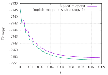
(a) Entropy vs $t$. $\Delta t=1/512$.

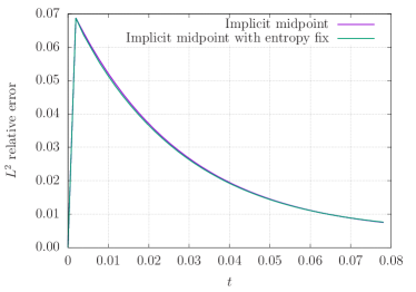
(b) $L^{2}$ relative error vs $t$. $\Delta t=1/512$.

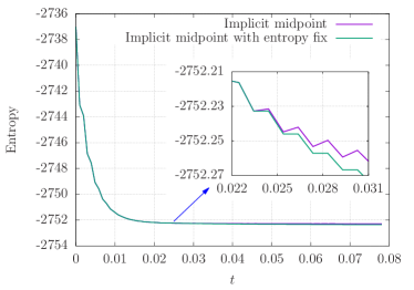
(c) Entropy vs $t$. $\Delta t=1/1024$.

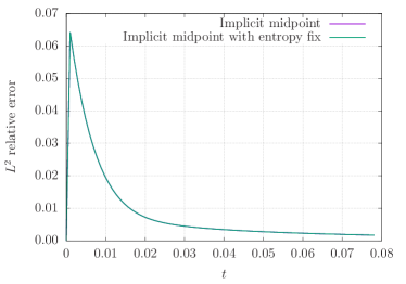
(d) $L^{2}$ relative error vs $t$. $\Delta t=1/1024$.

Figure 3: Example of the linear Fokker-Planck equation. Time evolution of the entropy $H(\boldsymbol{g})=\sum_{j=0}^{N-1}(g_{j}\log g_{j}-g_{j})M_{j}\Delta x$ and the $L^{2}$ relative error $\|\boldsymbol{g}-\boldsymbol{g}_{\rm exact}\|_{2}/\|\boldsymbol{g}_{\rm exact}\|_{2}=(\sum_{j=0}^{N-1}(g_{j}-g_{{\rm exact},j})^{2}M_{j}\Delta x)^{1/2}/(\sum_{j=0}^{N-1}(g_{{\rm exact},j})^{2}M_{j}\Delta x)^{1/2}$, where $\Delta x=1/64$, $\Delta t=1/512$ in the top two figures and $\Delta t=1/1024$ in the bottom two figures.

4.2 Nonlinear Boltzmann equation

In this example, we consider a nonlinear model introduced in [3], which results from a Fourier method for the spatially homogeneous Boltzmann equation. The governing equation reads

(47) $$\frac{\mathrm{d}f_{r}(t)}{\mathrm{d}t}=\sum_{p,q,s\in\mathcal{X}}A_{pq}^{rs}\left(f_{p}(t)f_{q}(t)-f_{r}(t)f_{s}(t)\right),\quad r\in\mathcal{X},$$

where $f_{r}$ represents the approximation of the distribution function on a uniform 3D lattice index set $\mathcal{X}=\{(r_{1},r_{2},r_{3})\mid r_{i}=0,\dots,M-1\text{ for }i=1,2,3\}$. In [3], the coefficients $A_{pq}^{rs}$ are determined in such a way that the semi-discrete scheme (47) decays the entropy. However, this property may not hold when the time is discretized.

In our experiment, we choose $M=17$, and the values of $A_{pq}^{rs}$ are given in Appendix B. The initial condition is taken as

$$f_{r}(0)=3.2+\sum_{j=1}^{10}\frac{j}{55}\left[\sin\Big{(}j\pi\big{(}\frac{r_{1}}{M}-\frac{1}{2}\big{)}\Big{)}+\sin\Big{(}j\pi\big{(}\frac{r_{2}}{M}-\frac{1}{2}\big{)}\Big{)}+\sin\Big{(}j\pi\big{(}\frac{r_{3}}{M}-\frac{1}{2}\big{)}\Big{)}\right].$$

We solve Eq. 47 by the forward Euler method with time step $\Delta t=0.0007$. The results are displayed in Fig. 4, from which we can see that the entropy fix method guarantees the monotonicity of the entropy. The numerical error is computed by comparison with the numerical solution computed with a smaller time step $\Delta t=0.000175$, with and without the entropy fix. It can be seen that the two error curves almost coincide with each other, meaning that the entropy fix does not ruin the numerical accuracy.

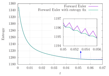
(a) Entropy vs $t$.

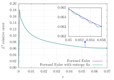
(b) $L^{2}$ relative error vs $t$.

Figure 4: Example of the nonlinear Boltzmann equation. Time evolution of the entropy $H(\boldsymbol{f})=\sum_{r\in\mathcal{X}}(f_{r}\log f_{r}-f_{r})\Delta v$ and the $L^{2}$ relative error $\|\boldsymbol{f}-\boldsymbol{f}_{\rm exact}\|_{2}/\|\boldsymbol{f}_{\rm exact}\|_{2}=(\sum_{r\in\mathcal{X}}(f_{r}-f_{{\rm exact},r})^{2}\Delta v)^{1/2}/(\sum_{r\in\mathcal{X}}(f_{{\rm exact},r})^{2}\Delta v)^{1/2}$, where $\Delta v=(3(3+\sqrt{2})/17)^{3}$ and $\Delta t=0.0007$. $\boldsymbol{f}_{\rm exact}$ is the numerical solution evaluated with time step $\Delta t=0.000175$.

5 Conclusions

This paper focuses on the entropic method for a conservative and positive system of ordinary differential equations. When the numerical solution at the next time step violates the monotonicity of entropy, our entropic method revises it by a linear interpolation to the constant state. The resulting scheme decays the entropy monotonically, while the order of local truncation error has a slight reduction in general. However, in some special cases, the numerical order is proved to be retained after entropic revision. Numerical experiments validate our results. Future work includes the extension of the entropic method to spatially inhomogeneous kinetic equations such as the Boltzmann equation and the radiative transfer equations.

Appendix A Proof of Lemma 3.20

This proof is composed of three steps:

1. $F(x,y,C)\geq F(x,\frac{1}{2C},C)$ for $0\leq x\leq\frac{1}{2}$, $C>1$ and $0\leq y\leq\frac{1}{2C}$;

2. $F(x,\frac{1}{2C},C)\geq\min(F(0,\frac{1}{2C},C),F(\frac{1}{2},\frac{1}{2C},C))$ for $0\leq x\leq\frac{1}{2}$ and $C>1$;

3. for any $C_{1}\in(0,1]$, there is $C_{2}>1$ depending on $C_{1}$ such that $F(0,\frac{1}{2C_{2}},C_{2})\geq\frac{1}{C_{1}}$ and $F(\frac{1}{2},\frac{1}{2C_{2}},C_{2})\geq\frac{1}{C_{1}}$.

A.1 First step

It is sufficient to show $\frac{\partial F(x,y,C)}{\partial y}\leq 0$ for $y\geq 0$, from which $F(x,y,C)\geq F(x,\frac{1}{2C},C)$ for $0\leq y\leq\frac{1}{2C}$. By the expression of $F(x,y,C)$ in Eq. 32, it could be calculated that

(48) $$\frac{\partial F(x,y,C)}{\partial y}=\frac{F_{1}(x,y,C)}{\left(h(x)-h(x+y)\right)^{2}},$$

where

$$F_{1}(x,y,C) =x\log\left(y+x\right)\left(\log\left(x\right)-\log\left(yC+x\right)\right)$$

$$+Cx\log\left(yC+x\right)\left(\log\left(y+x\right)-\log\left(x\right)\right)$$

$$+yC\left(\log\left(y+x\right)-\log\left(yC+x\right)\right).$$

Then we take the derivative of $F_{1}(x,y,C)$ with respect to $y$,

(49) $$\frac{\partial F_{1}(x,y,C)}{\partial y}=\frac{F_{2}(x,y,C)}{\left(y+x\right)\left(yC+x\right)},$$

where

$$F_{2}(x,y,C) =x^{2}\left(C^{2}\left(\log\left(y+x\right)-\log\left(x\right)\right)-\log\left(yC+x\right)+\log\left(x\right)\right)$$

$$+yCx\left(-2\log\left(yC+x\right)-C\left(-2\log\left(y+x\right)+\log\left(x\right)+1\right)\right)$$

$$+yCx\left(\log\left(x\right)+1\right)+y^{2}C^{2}\left(\log\left(y+x\right)-\log\left(yC+x\right)\right).$$

We continue to take the derivative of $F_{2}(x,y,C)$ w.r.t. $y$,

$$\frac{\partial F_{2}(x,y,C)}{\partial y}=C(C-1)x-C\left(-2Ch(x+y)+2h\left(x+Cy\right)+\left(C-1\right)h(x)\right).$$

When $C>1$, the convexity of $h(\cdot)$ implies

$$h(x+y)\leq\left(1-\frac{1}{C}\right)h(x)+\frac{1}{C}h(x+Cy).$$

Therefore,

$$-2Ch(x+y)+2h\left(x+Cy\right)+\left(C-1\right)h(x)\geq(1-C)h(x).$$

As a result,

$$\frac{\partial F_{2}(x,y,C)}{\partial y}\leq C(C-1)(h(x)+x)\leq 0,$$

where the last inequality utilizes $h(x)+x=x\log(x)\leq 0$ when $x\leq\frac{1}{2}$.

$\frac{\partial F_{2}(x,y,C)}{\partial y}\leq 0$ implies $F_{2}(x,y,C)$ is decreasing with respect to $y$ for fixed $x$ and $C$. At the same time, it is easy to verify that $F_{2}(x,0,C)=0$. Therefore, $F_{2}(x,y,C)\leq F_{2}(x,0,C)=0$ for $y\geq 0$.

From Eq. 49 and $F_{2}(x,y,C)\leq 0$, it is easy to get $\frac{\partial F_{1}(x,y,C)}{\partial y}\leq 0$, which means $F_{1}(x,y,C)$ is decreasing with respect to $y$ for fixed $x$ and $C$. Combining with $F_{1}(x,y,C)\mid_{y=0}=0$, we could find $F_{1}(x,y,C)\leq 0$ for $y\geq 0$.

Finally, plugging $F_{1}(x,y,C)\leq 0$ into Eq. 48, we could conclude that $\frac{\partial F(x,y,C)}{\partial y}\leq 0$ for $y\geq 0$.

A.2 Second step

For simplicity, We would like to introduce $G(x,C)$ to denote $F(x,\frac{1}{2C},C)$ as

(50) $$G(x,C)=F(x,\frac{1}{2C},C)=\frac{h(x+1/(2C))-h(x+1/2)}{h(x)-h(x+1/(2C))},$$

where the second equality is achieved by plugging $y=1/(2C)$ into Eq. 32. We will show that for fixed $C>1$, $G(x,C)$ is increasing and then decreasing for $0<x\leq\frac{1}{2}$, from which it is easy to see $G(x,C)\geq\min(G(0,C),G(\frac{1}{2},C))$. The idea is similar to the first step, which utilizes the sign of derivative.

By the expression of $G(x,C)$ in Eq. 50, a direct calculation shows

(51) $$\frac{\partial G(x,C)}{\partial x}=\frac{G_{1}(x,C)}{2C\left(h\left(x\right)-h\left(x+\frac{1}{2C}\right)\right)^{2}},$$

where

$$G_{1}(x,C) =C\left(\log\left(x+\frac{1}{2}\right)-1\right)\left(\log\left(x\right)-\log\left(x+\frac{1}{2C}\right)\right)$$

$$-\left(\log\left(x\right)-\log\left(x+\frac{1}{2}\right)\right)\left(\log\left(x+\frac{1}{2C}\right)-1\right).$$

Again, we taken the derivative of $G_{1}(x,C)$ w.r.t. $x$,

(52) $$\frac{\partial G_{1}(x,C)}{\partial x}=\frac{G_{2}(x,C)}{x\left(2x+1\right)\left(2Cx+1\right)},$$

where

$$G_{2}(x,C) =4C^{2}x^{2}\left(\log\left(x\right)-\log\left(x+\frac{1}{2C}\right)\right)-\log\left(x+\frac{1}{2C}\right)$$

$$+4Cx\left(\log\left(x+\frac{1}{2}\right)-\log\left(x+\frac{1}{2C}\right)\right)+1-C$$

$$+C\left(-4x^{2}\left(\log\left(x\right)-\log\left(x+\frac{1}{2}\right)\right)+\log\left(x+\frac{1}{2}\right)\right).$$

We continue to take the derivative of $G_{2}(x,C)$ w.r.t. $x$,

$$\frac{\partial G_{2}(x,C)}{\partial x}=8C\left(-Ch\left(x+\frac{1}{2C}\right)+\left(C-1\right)h(x)+h\left(x+\frac{1}{2}\right)\right).$$

The convexity of $h(\cdot)$ and $C>1$ implies

$$h\left(x+\frac{1}{2C}\right)\leq\left(1-\frac{1}{C}\right)h(x)+\frac{1}{C}h\left(x+\frac{1}{2}\right),$$

which means

$$-Ch\left(x+\frac{1}{2C}\right)+\left(C-1\right)h(x)+h\left(x+\frac{1}{2}\right)\geq 0.$$

Therefore, $\frac{\partial G_{2}(x,C)}{\partial x}\geq 0$ for $0<x\leq\frac{1}{2}$, meaning $G_{2}(x,C)$ is increasing w.r.t. $x$ for fixed $C$. On the other hand,

$$\lim_{x\to 0}G_{2}(x,C) =-\log\left(\frac{1}{C}\right)-C(1+\log(2))+1+\log(2)$$

$$\leq C-1-C(1+\log(2))+1+\log(2)=-\log(2)(C-1)<0,$$

and

$$G_{2}(\frac{1}{2},C)=-C-\left(C+1\right)^{2}\log\left(\frac{1}{2C}+\frac{1}{2}\right)-C\left(C-1\right)\log(2)+1\geq 0.$$

Therefore, for fixed $C$, there exists $0<G_{2}^{0}\leq\frac{1}{2}$, such that $G_{2}(x,C)\leq 0$ for $x\leq G_{2}^{0}$ and $G_{2}(x,C)\geq 0$ for $x\geq G_{2}^{0}$. The reason for $G_{2}(\frac{1}{2},C)\geq 0$ can be revealed from taking derivatives, i.e.,

$$\frac{\mathrm{d}G_{2}(\frac{1}{2},C)}{\mathrm{d}C}=\frac{1}{C}+3\log(2)-2\log\left(\left(\frac{C+1}{C}\right)^{(C+1)}\right),$$

$$\frac{\mathrm{d}^{2}G_{2}(\frac{1}{2},C)}{\mathrm{d}(C)^{2}}=\frac{2}{C}-\frac{1}{C^{2}}-2\log\left(\frac{1}{C}+1\right),$$

$$\frac{\mathrm{d}^{3}G_{2}(\frac{1}{2},C)}{\mathrm{d}(C)^{3}}=\frac{2}{C^{4}+C^{3}}>0.$$

$\frac{\mathrm{d}^{3}G_{2}(\frac{1}{2},C)}{\mathrm{d}(C)^{3}}>0$ implies $\frac{\mathrm{d}^{2}G_{2}(\frac{1}{2},C)}{\mathrm{d}(C)^{2}}$ is increasing, which gives

$$\frac{\mathrm{d}^{2}G_{2}(\frac{1}{2},C)}{\mathrm{d}(C)^{2}}\leq\lim_{C\to\infty}\frac{\mathrm{d}^{2}G_{2}(\frac{1}{2},C)}{\mathrm{d}(C)^{2}}=0.$$

Therefore, $\frac{\mathrm{d}G_{2}(\frac{1}{2},C)}{\mathrm{d}C}$ is decreasing,

$$\frac{\mathrm{d}G_{2}(\frac{1}{2},C)}{\mathrm{d}C}\geq\lim_{C\to\infty}\frac{\mathrm{d}G_{2}(\frac{1}{2},C)}{\mathrm{d}C}=3\log(2)-2>0.$$

As a result, $G_{2}(\frac{1}{2},C)$ is increasing for $C>1$ and $G_{2}(\frac{1}{2},C)\geq G_{2}(\frac{1}{2},1)=0$.

Since $G_{2}(x,C)\leq 0$ for $x\leq G_{2}^{0}$ and $G_{2}(x,C)\geq 0$ for $x\geq G_{2}^{0}$, we could find $G_{1}(x,C)$ is decreasing on $(0,G_{2}^{0}]$ and increasing on $[G_{2}^{0},\frac{1}{2}]$ from Eq. 52. On the other hand, due to $C>1$ and $\log(C)\leq C-1$,

$$\lim_{x\to 0}G_{1}(x,C)=\lim_{x\to 0}\left((1-C)\log(2)+\log(C)+1-C\right)\log(x)=\infty.$$

Together with

$$G_{1}(\frac{1}{2},C)=\left(C+\log(2)\right)\log\left(\frac{1}{C}+1\right)-\log(2)(1+\log(2))\leq 0,$$

we could get for fixed $C$, there exists $0<G_{1}^{0}\leq\frac{1}{2}$, such that $G_{1}(x,C)\geq 0$ for $x\leq G_{1}^{0}$ and $G_{1}(x,C)\leq 0$ for $x\geq G_{1}^{0}$. Similar to $G_{2}(\frac{1}{2},C)$, the reason for $G_{1}(\frac{1}{2},C)\leq 0$ can be revealed from taking derivatives.

$$\frac{\mathrm{d}G_{1}(\frac{1}{2},C)}{\mathrm{d}C}=\log\left(\frac{1}{C}+1\right)-\frac{C+\log(2)}{C(1+C)},$$

$$\frac{\mathrm{d}^{2}G_{1}(\frac{1}{2},C)}{\mathrm{d}(C)^{2}}=\frac{C(\log(4)-1)+\log(2)}{C^{2}\left(C+1\right){}^{2}}>0,$$

which means $\frac{\mathrm{d}G_{1}(\frac{1}{2},C)}{\mathrm{d}C}$ is increasing w.r.t. $C$. Therefore,

$$\frac{\mathrm{d}G_{1}(\frac{1}{2},C)}{\mathrm{d}C}\leq\lim_{C\to\infty}\frac{\mathrm{d}G_{1}(\frac{1}{2},C)}{\mathrm{d}C}=0,$$

which implies $G_{1}(\frac{1}{2},C)$ is decreasing for $C>1$. Hence, $G_{1}(\frac{1}{2},C)\leq G_{1}(\frac{1}{2},1)=0$.

Using Eq. 51, together with $G_{1}(x,C)\geq 0$ for $x\leq G_{1}^{0}$ and $G_{1}(x,C)\leq 0$ for $x\geq G_{1}^{0}$, we could get $G(x,C)$ is increasing on $(0,G_{1}^{0}]$ and then decreasing on $[G_{1}^{0},\frac{1}{2}]$ with respect to $x$.

A.3 Third step

With the notation in Eq. 50, we would like to evaluate $G(0,C)$ and $G(1/2,C))$ one by one.

On the one hand, for $G(0,C)$, since $\log(2C)\leq 2\sqrt{C}-1$ for $C\geq 1$ (which can be proved by the monotonicity of $\log(2C)-2\sqrt{C}+1$), it holds that

$$G(0,C)=\frac{h(\frac{1}{2C})-h(\frac{1}{2})}{h(0)-h(\frac{1}{2C})}=\frac{C(1+\log(2))}{\log\left(2C\right)+1}-1\geq\frac{1+\log(2)}{2}\sqrt{C}-1.$$

Therefore, for any $C_{1}\in(0,1]$, we could take $C_{2}=\left(\frac{2(1+C_{1})}{C_{1}(1+\log(2))}\right)^{2}$, which gives $G(0,C_{2})\geq\frac{1}{C_{1}}$. Furthermore, it is easy to find $C_{2}=\left(\frac{2}{(1+\log(2))}\right)^{2}\left(\frac{1+C_{1}}{C_{1}}\right)^{2}\geq\frac{16}{(1+\log(2))^{2}}$ since $\frac{1+C_{1}}{C_{1}}\geq 2$ for $0<C_{1}\leq 1$.

On the other hand, for $G(\frac{1}{2},C)$,

$$G(\frac{1}{2},C)=\frac{h(\frac{1}{2}+\frac{1}{2C})-h(1)}{h(\frac{1}{2})-h(\frac{1}{2}+\frac{1}{2C})}=\frac{C+\left(C+1\right)\left(\log\left(\frac{1}{C}+1\right)-\log(2)\right)-1}{-\left(C+1\right)\log\left(\frac{1}{C}+1\right)+1+\log(2)}.$$

Since $\left(C+1\right)\log\left(\frac{1}{C}+1\right)\geq 1$, it holds that when $C\geq\frac{16}{(1+\log(2))^{2}}$, the numerator

$$C+\left(C+1\right)\left(\log\left(\frac{1}{C}+1\right)-\log(2)\right)-1\geq(1-\log(2))C-\log(2)>0.$$

Then, we could utilize $\left(C+1\right)\log\left(\frac{1}{C}+1\right)\geq 1$ in the denominator of $G(\frac{1}{2},C)$ and get

$$G(\frac{1}{2},C)\geq\frac{(1-\log(2))C-\log(2)}{\log(2)}.$$

Therefore, we could take $C_{2}=\max(\frac{16}{(1+\log(2))^{2}},\frac{(C_{1}+1)\log(2)}{C_{1}(1-\log(2))})$ to get $G(\frac{1}{2},C_{2})\geq\frac{1}{C_{1}}$.

Combining the results of $G(0,C_{2})$ and $G(\frac{1}{2},C_{2})$, we could conclude that for any $C_{1}\in(0,1]$, there exists $C_{2}=\max\Big{(}\left(\frac{2(1+C_{1})}{C_{1}(1+\log(2))}\right)^{2},\frac{(C_{1}+1)\log(2)}{C_{1}(1-\log(2))}\Big{)}$ such that $G(0,C_{2})\geq\frac{1}{C_{1}}$ and $G(\frac{1}{2},C_{2})\geq\frac{1}{C_{1}}$. In fact, for $C_{1}\in(0,1]$, $\left(\frac{2(1+C_{1})}{C_{1}(1+\log(2))}\right)^{2}\geq\frac{(C_{1}+1)\log(2)}{C_{1}(1-\log(2))}$. The derivative of their difference is

$$\frac{\mathrm{d}}{\mathrm{d}C_{1}}\left(\left(\frac{2(1+C_{1})}{C_{1}(1+\log(2))}\right)^{2}-\frac{(C_{1}+1)\log(2)}{C_{1}(1-\log(2))}\right)$$

$$= \frac{-C_{1}\left(-8+\log^{3}(2)+2\log^{2}(2)+\log(512)\right)+8-8\log(2)}{C_{1}^{3}(\log(2)-1)(1+\log(2))^{2}}.$$

Since $\left(-8+\log^{3}(2)+2\log^{2}(2)+\log(512)\right)<0$, the above numerator is greater than $8-8\log(2)$ for $0<C_{1}\leq 1$, which is positive. Combining with the negative denominator, the above derivative is negative, therefore,

$$\left(\frac{2(1+C_{1})}{C_{1}(1+\log(2))}\right)^{2}-\frac{(C_{1}+1)\log(2)}{C_{1}(1-\log(2))}\geq\left(\frac{4}{1+\log(2)}\right)^{2}-\frac{2\log(2)}{1-\log(2)}>0.$$

As a result, $\max\Big{(}\left(\frac{2(1+C_{1})}{C_{1}(1+\log(2))}\right)^{2},\frac{(C_{1}+1)\log(2)}{C_{1}(1-\log(2))}\Big{)}=\left(\frac{2(1+C_{1})}{C_{1}(1+\log(2))}\right)^{2}$, and the third step is proved with $C_{2}=\left(\frac{2(1+C_{1})}{C_{1}(1+\log(2))}\right)^{2}$.

Appendix B Coefficients in Eq. Eq. 47

The values of $A_{pq}^{rs}$ are given by

(53) $$A_{pq}^{rs}=\frac{1}{M^{9}}\sum_{l,h,k\in K}\hat{B}_{M}^{\sigma}(h-k,l-k)E_{-l}(p-s)E_{-h}(q-s)E_{k}(r-s),$$

where $K$ is defined as $K=\{k\mid k=(k_{1},k_{2},k_{3}),-m\leq k_{1},k_{2},k_{3}\leq m\}$ with $M=2m+1$, and $E_{k}(v)=\exp(\frac{\mathbf{i}\pi}{T}k\cdot v)$ is the Fourier basis on the period $[-T,T]^{3}$. The kernel function $\hat{B}_{M}^{\sigma}(\cdot,\cdot)$ are defined by

$$\hat{B}_{M}^{\sigma}(i,j):=\hat{B}(i\bmod M,j\bmod M)\sigma_{M}(i\bmod M)\sigma_{M}(j\bmod M),$$

where $\bmod$ is the symmetric modulo function such that each component of $i\bmod M$ ranges from $-m$ to $m$, and $\sigma_{M}(i)=\tilde{\sigma}_{M}(i_{1})\tilde{\sigma}_{M}(i_{2})\tilde{\sigma}_{M}(i_{3})$ where $\tilde{\sigma}_{M}(\beta)$ is the one-dimensional modified Jackson filter [12] given by

$$\tilde{\sigma}_{M}(\beta)=\frac{(m+1-|\beta|)\cos\left(\frac{\pi|\beta|}{m+1}\right)+\sin\left(\frac{\pi|\beta|}{m+1}\right)\cot\left(\frac{\pi}{m+1}\right)}{m+1}.$$

In the example in Section 4.2, we adopt the kernel modes for the case of the Maxwell molecules presented in [9] with

$$\hat{B}(k,l):=\int_{0}^{1}r^{2}\operatorname{Sinc}(\xi r)\operatorname{Sinc}(\eta r)\,\mathrm{d}r=\frac{(\xi+\eta)\sin(\xi-\eta)-(\xi-\eta)\sin(\xi+\eta)}{2\xi\eta(\xi^{2}-\eta^{2})},$$

where $\xi=|k+l|\lambda\pi,\eta=|k-l|\lambda\pi$, and $\lambda=2/(3+\sqrt{2}$). In the numerical simulation, we take $M=17$ and $T=3/\lambda$.

References

- [1] R. Bailo, J. A. Carrillo, and J. Hu, Fully discrete positivity-preserving and energy-dissipating schemes for aggregation-diffusion equations with a gradient flow structure, Comm. Math. Sci., 18 (2020), pp. 1259–1303.
- [2] C. Buet and S. Cordier, Numerical analysis of conservative and entropy schemes for the Fokker–Planck–Landau equation, SIAM J. Numer. Anal., 36 (2006), pp. 953–973.
- [3] Z. Cai, Y. Fan, and L. Ying, An entropic fourier method for the Boltzmann equation, SIAM Journal on Scientific Computing, 40 (2018), pp. A2858–A2882, https://doi.org/10.1137/17M1127041.
- [4] S. Chow, L. Dieci, and W. Li, Entropy dissipation semi-discretization schemes for Fokker–Planck equations, J. Dyn. Diff. Equat., 31 (2019), pp. 765–792.
- [5] R. M. Corless, G. H. Gonnet, D. E. G. Hare, D. J. Jeffrey, and D. E. Knuth, On the Lambert function, Advances in Computational Mathematics, 5 (1996), pp. 329–359.
- [6] P. Degond and B. Lucquin-Desreux, An entropy scheme for the fokker-planck collision operator of plasma kinetic theory, Numer. Math., 68 (1994), pp. 239–262.
- [7] D. Goldstein, B. Strutevant, and J. E. Broadwell, Investigations of the Motion of Discrete-Velocity Gases, AIAA, 1989, pp. 100–117.
- [8] A. Hoorfar and M. Hassani, Inequalities on the Lambert function and hyperpower function, J. Inequal. Pure and Appl. Math, 9 (2008), pp. 1–5.
- [9] L. Pareschi and G. Russo, Numerical solution of the Boltzmann equation I: Spectrally accurate approximation of the collision operator, SIAM J. Numer. Anal., 37 (2000), pp. 1217–1245.
- [10] L. Pareschi and M. Zanella, Structure preserving schemes for nonlinear Fokker–Planck equations and applications, J. Sci. Compute., 74 (2018), pp. 1575–1600.
- [11] A. Ruszczyński, Nonlinear optimization, Princeton University Press, Princeton, 2006.
- [12] A. Weiße, G. Wellein, A. Alvermann, and H. Fehske, The kernel polynomial method, Rev. Mod. Phys., 78 (2006), pp. 275–306, https://doi.org/10.1103/RevModPhys.78.275, https://link.aps.org/doi/10.1103/RevModPhys.78.275.