Identifiability and estimation of meta-elliptical copula generators

Abstract

Meta-elliptical copulas are often proposed to model dependence between the components of a random vector. They are specified by a correlation matrix and a map $g$, called density generator. While the latter correlation matrix can easily be estimated from pseudo-samples of observations, the density generator is harder to estimate, especially when it does not belong to a parametric family. We give sufficient conditions to non-parametrically identify this generator. Several nonparametric estimators of $g$ are then proposed, by M-estimation, simulation-based inference, or by an iterative procedure available in the R package ElliptCopulas. Some simulations illustrate the relevance of the latter method.

1 Introduction

Elliptically contoured distributions are usual semi-parametric extensions of multivariate Gaussian or Student distributions. They correspond to continuous distributions on $\mbox{$\mathbb{R}$}^{d}$ whose isodensity curves (with respect to the Lebesgue measure) are ellipsoids: see, e.g., [7, 14, 21, 27]. To be specific, let ${\bf X}$ be a random vector in $\mbox{$\mathbb{R}$}^{d}$ whose elliptical distribution is parameterized by a vector ${\bm{\mu}}\in\mbox{$\mathbb{R}$}^{d}$, a positive definite matrix ${\bm{\Omega}}=[\Omega_{i,j}]_{1\leq i,j\leq d}$ and a measurable function $g:\mbox{$\mathbb{R}$}^{+}\rightarrow\mbox{$\mathbb{R}$}^{+}\cup\{+\infty\}$. Its density with respect to the Lebesgue measure in $\mbox{$\mathbb{R}$}^{d}$ is

$$f_{{\bf X}}({\bf x})={|{\bm{\Omega}}|}^{-1/2}g\left(({\bf x}-{\bm{\mu}})^{\top}\,{\bm{\Omega}}^{-1}\,({\bf x}-{\bm{\mu}})\right),\;{\bf x}\in\mbox{$\mathbb{R}$}^{d}.$$ (1)

This distribution is denoted $\mbox{$\mathcal{E}$}_{d}({\bm{\mu}},{\bm{\Omega}},g)$ and its cumulative distribution function by $H_{g,{\bm{\Omega}},d}$. To specify the law of the random vector ${\bf X}$, we will write ${\bf X}\sim\mbox{$\mathcal{E}$}_{d}({\bm{\mu}},{\bm{\Omega}},g)$. The map $g$ is called “density generator”, or simply “generator”. By integration of (1), a density generator of an elliptical vector satisfies the constraint

$$s_{d}\int_{0}^{\infty}r^{d-1}g(r^{2})\,dr=s_{d}\int_{0}^{\infty}t^{d/2-1}g(t)\,dt/2=1,$$ (2)

where $s_{d}:=2\pi^{d/2}/\Gamma(d/2)$ is the surface area of the unit ball in $\mbox{$\mathbb{R}$}^{d}$, $d\geq 2$ ($s_{1}=2$). Conversely, any nonnegative function $g$ that satisfies (2) can be used as the density generator of an elliptical distribution. For example, the density generator of a Gaussian distribution is $g_{Gauss}(u):=\exp(-u/2)/(2\pi)^{d/2}$.

Remark 1.

It is possible to define elliptical distributions with singular matrices ${\bm{\Omega}}$: see [7]. In such cases, ${\bm{\lambda}}^{\top}{\bf X}=0$ a.s. for some vector ${\bm{\lambda}}$ in $\mbox{$\mathbb{R}$}^{d}$, and the law of ${\bf X}$ is supported on an affine subspace of $\mbox{$\mathbb{R}$}^{d}$. Such “degenerate” cases will not be considered in this paper.

A $d$-dimensional copula $C$ is said meta-elliptical (or simply “elliptical”) if there exists an elliptical distribution in $\mbox{$\mathbb{R}$}^{d}$ whose copula is $C$. Due to the invariance of copulas by location-scale transforms, an elliptical copula depends on a generator and a correlation matrix only. Indeed, for any ${\bf X}\sim\mbox{$\mathcal{E}$}_{d}({\mathbf{0}},{\bm{\Omega}},g)$, set ${\bf Y}:=(X_{1}/\sqrt{\Omega_{1,1}},\ldots,X_{d}/\sqrt{\Omega_{d,d}})^{\top}$. Then, ${\bf Y}\sim\mbox{$\mathcal{E}$}_{d}({\mathbf{0}},{\bm{\Sigma}},g)$ for a correlation matrix ${\bm{\Sigma}}:=[\Omega_{i,j}/(\Omega_{i,i}\Omega_{j,j})^{1/2}]$. Obviously, the meta-elliptical copulas of ${\bf X}$ and ${\bf Y}$ are the same. Thus, for any correlation matrix ${\bm{\Sigma}}$, denote by $\mbox{$\mathcal{M}$}\mbox{$\mathcal{E}$}_{d}({\bm{\Sigma}},g)$ the (unique) meta-elliptical copula that corresponds to the elliptical distribution $\mbox{$\mathcal{E}$}_{d}({\mathbf{0}},{\bm{\Sigma}},g)$. More generally, this copula corresponds to the elliptical distributions $\mbox{$\mathcal{E}$}_{d}(\mu,{\bm{\Omega}},g)$ for any $\mu,{\bm{\Omega}}$, such that ${\bm{\Sigma}}$ is the correlation matrix associated to ${\bm{\Omega}}$.

A trans-elliptical distribution [34, 35] is a distribution whose copula is meta-elliptical. Trans-elliptical distributions ([13]) extend elliptical distributions, by allowing the associated margins to be arbitrarily specified. For any correlation matrix ${\bm{\Sigma}}$, we will denote by $\mbox{$\mathcal{T}$}\mbox{$\mathcal{E}$}_{d}({\bm{\Sigma}},g,F_{1},\dots,F_{d})$ the trans-elliptical distribution whose copula is $\mbox{$\mathcal{M}$}\mbox{$\mathcal{E}$}_{d}({\bm{\Sigma}},g)$ and marginal cdfs’ are $F_{1},\dots,F_{d}$.

The probabilistic properties of meta-elliptical copulas and their statistical analysis have been studied in several papers in the literature: their conditional distributions and dependence measures [13], the estimation of the correlation matrix $\Sigma$ [52], stochastic ordering [1], sampling methods [51], their tail dependence function [28, 29, 30], their use semi-parametric regressions [54] or some goodness-of-fit tests [24, 25], their relationships with partial and conditional correlations [31], etc., are notable contributions. Thanks to Sklar’s theorem, meta-elliptical copulas can be used as key components of many flexible multivariate models, far beyond elliptically-distributed random vectors. Moreover, the literature has considered parametric families of generators that include the popular Gaussian and/or Student copulas as particular cases, with practical applications in hydrology [17, 46], risk management [10, 16], econometrics [44], biology, etc.

To the best of our knowledge, all these papers assume the generator of a meta-elliptical copula is known, possibly up to finite dimensional parameter. Thus, the problem of estimating $g$ itself is bypassed. For instance, [17] proposed a graphical tool to select a “well-suited” generator among a finite set of potential generators. Approximations of meta-elliptical copulas are proposed in [48] through projection pursuit techniques but the consistency of the proposed algorithm seems to occur only under very restrictive conditions. Actually, a general nonparametric estimation of the generator $g$ is problematic. As noticed in Genest et al. [17] : “The estimation of g is more complex, considering that it is a functional parameter. Indeed, a rigorous approach to this problem has yet to be developed. Financial applications to date have simply treated g as fixed; however, several possible choices of g have often been considered to assess the robustness of the conclusions derived from the model.” Therefore, until now, no nonparametric consistent estimator of $g$ seems to be available in the literature. This should not be surprising. Indeed, a preliminary point would be to state the identifiability of $g$ from the knowledge of the underlying copula. This result is far from obvious and is one of the main contributions of our work.

Let us explain why this is the case. As recalled in the appendix, all margins of a distribution $\mbox{$\mathcal{E}$}_{d}({\mathbf{0}},{\bm{\Sigma}},g)$ have the same density $f_{g}$, where, for every $t\in\mbox{$\mathbb{R}$}$,

$$f_{g}(t)=\frac{\pi^{(d-1)/2}}{\Gamma((d-1)/2)}\int_{0}^{+\infty}g(t^{2}+s)s^{(d-3)/2}\,ds.$$ (3)

Note that $f_{g}$ is even. For notational convenience, we do not write the dependency of $f_{g}$ on the dimension $d$. Set its marginal cdfs’ $F_{g}(x)=\int_{-\infty}^{x}f_{g}(t)\,dt$ for every real number $x$, and its quantile function $Q_{g}(u)=\inf\{x;F_{g}(x)\geq u\}$, $u\in[0,1]$. By Sklar’s theorem, our meta-elliptical distribution $C\sim\mbox{$\mathcal{M}$}\mbox{$\mathcal{E}$}_{d}({\bm{\Sigma}},g)$ is given by

$$C({\bf u}) =H_{g,{\bm{\Sigma}},d}\big{(}Q_{g}(u_{1}),\ldots,Q_{g}(u_{d})\big{)}={|{\bm{\Sigma}}|}^{-1/2}{\int_{-\infty}^{Q_{g}(u_{1})}\cdots\int_{-\infty}^{Q_{g}(u_{d})}}g\big{(}{\bf x}^{\top}{\bm{\Sigma}}^{-1}{\bf x}\big{)}\,d{\bf x},$$ (4)

for every ${\bf u}\in(0,1)^{d}$. Hence, the associated meta-elliptical copula density with respect to the Lebesgue measure exists and may be defined as

$$c({\bf u}):=\frac{g\big{(}\vec{Q}_{g}({\bf u}){\bm{\Sigma}}^{-1}\vec{Q}_{g}({\bf u})^{\top}\big{)}}{|{\bm{\Sigma}}|^{1/2}\prod_{k=1}^{d}f_{g}\big{(}Q_{g}(u_{k})\big{)}},\;\;\text{where }\vec{Q}_{g}({\bf u}):=\big{[}Q_{g}(u_{1}),\ldots,Q_{g}(u_{d})\big{]},$$ (5)

for every ${\bf u}\in[0,1]^{d}$. The latter density and cumulative distribution function will be denoted by $c_{g}$ and $C_{g}$ respectively, when we want to stress its dependence with respect to $g$.

Concerning the inference of meta-elliptical copulas, the usual estimator of the matrix ${\bm{\Sigma}}$ has been known for a long time and is based on empirical Kendall’s tau (see below). When one observes i.i.d. realizations of elliptically-distributed random vectors, several estimators of the generator $g$ have been proposed in the literature (see our appendix). This paper is related to the same purpose, but for trans-elliptical distributions, or, equivalently, for meta-elliptical copulas. In such a case, the inference of $g$ is more difficult than for elliptical laws because copula densities depend on $g$ through a highly nonlinear and complex relationship. Moreover, it is not known whether the mapping $g\mapsto c_{g}$ is one-to-one. To the best of our knowledge, this problem has never been tackled in the literature. Authors only rely on ad-hoc chosen generators, or on parametric families of generators.

In Section 2, we give sufficient conditions for the identifiability of the generator of a meta-elliptical copula. Estimation procedures of $g$ are proposed in Section 3. They allow the nonparametric estimation of an assumed trans-elliptical distribution, because ${\bm{\Sigma}}$ and its margins are easily estimated beside. Section 3.1 proposes a penalized M-estimation of $g$, when a simulation-based estimator is given in Section 3.2. Section 3.3 states a numerical iterative procedure to evaluate $g$. It will be called MECIP, as “Meta-Elliptical Copula Iterative Procedure”. Its performances are evaluated in Section 4 and it is implemented in the R package ElliptCopulas [9].

2 Identifiability of meta-elliptical copulas

Consider a meta-elliptical copula $C=\mbox{$\mathcal{M}$}\mbox{$\mathcal{E}$}_{d}({\bm{\Sigma}},g)$ where ${\bm{\Sigma}}$ is a correlation matrix and $g$ satisfies the usual normalization constraint (2). The question is to know whether the latter parameterization is unique. Strictly speaking, this is the same question as for trans-elliptical distributions when their margins are known.

For any meta- or trans-elliptical distribution, the correlation matrix ${\bm{\Sigma}}$ is identifiable. Indeed, it is well-known there exists a nice relationship between its components and the underlying Kendall’s tau: $\Sigma_{k,l}=\sin(\pi\tau_{k,l}/2)$, $k\neq l$, where $\tau_{k,l}$ is the Kendall’s tau between $X_{k}$ and $X_{l}$. See [52] and the references therein, for instance. Since every $\tau_{k,l}$ is uniquely defined by the underlying copula of ${\bf X}$, this is still the case for ${\bm{\Sigma}}$ too.

Proposition 1.

If ${\bf U}\sim\mbox{$\mathcal{M}$}\mbox{$\mathcal{E}$}_{d}({\bm{\Sigma}},g)$ and ${\bf U}\sim\mbox{$\mathcal{M}$}\mbox{$\mathcal{E}$}_{d}(\tilde{\bm{\Sigma}},\tilde{g})$ where ${\bm{\Sigma}}$ and $\tilde{\bm{\Sigma}}$ are two correlation matrices, then ${\bm{\Sigma}}=\tilde{\bm{\Sigma}}$.

Note that it is possible to have $g\neq\tilde{g}$ due to the non-uniqueness of meta-elliptical copula generators (see Proposition 2 below). If ${\bf X}$ is a trans-elliptical random vector, the inference of the matrix ${\bm{\Sigma}}$ can be done independently of the margins. The estimated matrix $\hat{\bm{\Sigma}}:=[\hat{\Sigma}_{k,l}]$ is given by $\hat{\Sigma}_{k,l}:=\sin(\pi\hat{\tau}_{k,l}/2)$, $k\neq l$, and $\hat{\Sigma}_{k,k}=1$, introducing empirical Kendall’s tau

$$\hat{\tau}_{k,l}:=\frac{2}{n(n-1)}\sum_{1\leq i<j\leq n}\text{sign}(X_{i,k}-X_{j,k})\times\text{sign}(X_{i,l}-X_{i,l}),\;\;k\neq l.$$

Since it is not guaranteed that $\hat{\bm{\Sigma}}$ is a correlation matrix, this can be imposed by projection techniques ([43, Section 8.7.2.1], e.g.). Hereafter, we require that $\hat{\bm{\Sigma}}$ is invertible.

Having tackled the identifiability and the estimation problem of ${\bm{\Sigma}}$, the problem is reduced to the following one: let $g$ and $\bar{g}$ be two density generators of meta-elliptical copulas on $[0,1]^{d}$ such that $c_{g}=c_{\bar{g}}$, with the previous notations. Does it imply that $g=\bar{g}$ almost everywhere?

Remark 2.

There is a one-to-one mapping between generators $g$ of meta-elliptical copulas and the so-called univariate densities $f_{g}$, as given in (3), once the underlying copula density $c$ is known. Indeed, since ${\bm{\Sigma}}^{-1}$ is definite positive, its diagonal elements are positive. Then, invoke (5) with $\vec{Q}_{g}({\bf u}):=\big{[}x,0,\ldots,0\big{]}$ for some arbitrary $x\in\mbox{$\mathbb{R}$}$. Since $f_{g}$ is even, $F_{g}(0)=1/2$ and $f_{g}(0)\neq 0$ by (3). This yields $g(\gamma x^{2})=|{\bm{\Sigma}}|^{1/2}f_{g}(0)^{d-1}f_{g}(x)c\big{(}F_{g}(x),1/2,\ldots,1/2\big{)}$ for every $x$ and some known positive constant $\gamma$. This means the map $g\mapsto f_{g}$ is invertible, restricting ourselves to meta-elliptical copula generators. In other words, since copula densities are nonparametrically identifiable, the identifiability problem of $g$ or of $f_{g}$ are the same. But, since $f_{g}$ can be (nonparametrically) identified only in the case of elliptical distributions, this does not prove the identifiability of $g$ for general meta-elliptical/trans-elliptical distributions.

Recall that elliptical distributions $\mbox{$\mathcal{E}$}_{d}({\bm{\mu}},{\bm{\Omega}},g)$ are not identifiable in general without any identifiability constraint (see Proposition 6 in the appendix). Therefore, most authors impose a condition such as $\text{Cov}({\bf X})={\bm{\Omega}}$ (when ${\bf X}$ has finite second moments) or $\text{Tr}({\bm{\Omega}})=1$ (in the general case). To deal with meta-elliptical copulas, we are facing similar problems. Indeed, such distributions are never identifiable without identifiability constraints, as proven in the next proposition.

Proposition 2.

Let ${\bm{\Sigma}}$ be a positive definite correlation matrix and $g$ be a density generator of a meta-elliptical copula on $[0,1]^{d}$. Then, for any $a>0$, $\mbox{$\mathcal{M}$}\mbox{$\mathcal{E}$}_{d}({\bm{\Sigma}},g)=\mbox{$\mathcal{M}$}\mbox{$\mathcal{E}$}_{d}({\bm{\Sigma}},g_{a})$ by setting $g_{a}(t):=a^{d/2}g(a\times t)$.

Proof of Proposition 2.

By (3), we easily get $f_{g_{a}}(t)=\sqrt{a}f_{g}(\sqrt{a}t)$ for every $t$. Deduce $F_{g_{a}}(x)=F_{g}(\sqrt{a}x)$ and $Q_{g_{a}}(u)=Q_{g}(u)/\sqrt{a}$ for every $t$ and $u$. Then, applying (5), we check that the copula densities associated to $g$ and $g_{a}$ respectively are the same. ∎

Therefore, for a given meta-elliptical copula, its generator $g$ has to satisfy at least another constraint in addition to (2), to be uniquely defined. We will prove that the generator of any elliptical copula is identifiable under some regularity conditions. This is one of the main contributions of our work. Before, we need our density generators to be sufficiently regular so that the associated univariate densities $f_{g}$ are differentiable. This is guaranteed by the next assumption.

Condition 1.

Set $a_{g}:=\sup\{t\,|\,t>0,g(t^{2})>0\}\in\bar{}\mbox{$\mathbb{R}$}_{+}$. The map $t\mapsto g(t^{2})$ from $\mathbb{R}$ to $\mbox{$\mathbb{R}$}^{+}$ is strictly positive and differentiable on $(-a_{g},a_{g})$. Moreover, the map $t\mapsto\int_{0}^{+\infty}g(t^{2}+r^{2})r^{d-2}\,dr$ is finite and differentiable on $\mathbb{R}$.

As a consequence, $\{t\,|\,g(t)>0\}$ (resp. $\{t\,|\,f_{g}(t)>0\}$) is equal to the interval $(-a_{g}^{2},a_{g}^{2})$ (resp. $(-a_{g},a_{g})$), possibly including the boundaries. Thus, we do not allow generators whose supports exhibit “holes”, such as sums of indicator functions that are related to disjoint subsets. The forbidden models correspond to meta-elliptical copulas whose densities are zero in some “cavities” that look like “distorted rings” (when plotted on $[0,1]^{d}$). Such features can easily be identified by plotting nonparametric estimates of $c_{g}$ as a preliminary stage. They are also unlikely to happen in practical applications.

Denote by ${\mathcal{G}}$ the set of density generators $g$ that satisfy Condition 1, in addition to (2). They will be called “regular density generators”. Moreover, denote by $c_{i,j}$ the map from $[0,1]^{2}$ to $\mathbb{R}$ that is equal to the copula density $c$, when all its arguments are equal to $1/2$, except the $i$-th and the $j$-th.

Proposition 3.

Consider a meta-elliptical random vector ${\bf U}\sim\mbox{$\mathcal{M}$}\mbox{$\mathcal{E}$}_{d}({\bm{\Sigma}},g)$, where the correlation matrix ${\bm{\Sigma}}$ is not the identity matrix ${\bf I}_{d}$. Let $i$ and $j$ be two different indices in $\{1,\ldots,d\}$ for which the $(i,j)$-component of ${\bm{\Sigma}}^{-1}$ is not zero. Assume that $c_{i,j}$ has finite first-order partial derivatives on $(0,1)^{2}$. Moreover, the maps $u\mapsto\partial_{k}\ln c_{i,j}(u,1/2)$, $k\in\{1,2\}$, are locally Lipschitz on $(0,1)$. Consider two couples $({\bm{\Sigma}}_{k},g_{k})$, $g_{k}\in{\mathcal{G}}$, $k\in\{1,2\}$, that induce the same law of ${\bf U}$ and that both satisfy

$$b:=\frac{\pi^{(d-1)/2}}{\Gamma((d-1)/2)}\int_{0}^{+\infty}g_{k}(s)s^{(d-3)/2}\,ds,$$ (6)

for a given positive real number $b$. Then these couples are essentially unique: ${\bm{\Sigma}}_{1}={\bm{\Sigma}}_{2}$; the supports of $g_{1}$ and $g_{2}$ are the same interval (except possibly at its boundaries), and $g_{1}=g_{2}$ on the interior of their common support.

Therefore, $b$ can be arbitrarily chosen. For any generator $g$, it is always possible to find a version $\tilde{g}$ such that $\mbox{$\mathcal{M}$}\mbox{$\mathcal{E}$}_{d}({\bm{\Sigma}},g)=\mbox{$\mathcal{M}$}\mbox{$\mathcal{E}$}_{d}({\bm{\Sigma}},\tilde{g})$ for all matrices ${\bm{\Sigma}}$, and such that $b(\tilde{g})=1$. An explicit procedure to build $\tilde{g}$ is given in Algorithm 1. Note that (6) means $f_{g_{1}}(0)=f_{g_{2}}(0)=b$. By (3), $f_{g_{1}}=f_{g_{2}}$ and $F_{g_{1}}=F_{g_{2}}$ everywhere, implying $C_{g_{1}}=C_{g_{2}}$ everywhere by (4). Condition 1 implies $g(0)>0$, that is equivalent to $c(1/2,1/2,\ldots,1/2)>0$ (see (13) in the proof). The latter condition seems to be weak, particularly under a practical perspective: copulas that have no mass at the center of their support can be considered as “pathological”.

Therefore, for a given elliptical copula and if ${\bm{\Sigma}}\neq{\bf I}_{d}$, there “most often” exists a unique regular density generator $g$ for which the constraints (6) and $s_{d}\int_{0}^{\infty}t^{d/2-1}g(t)\,dt/2=1$ are both satisfied. In other words, two moment-type conditions are sufficient to uniquely identify the generator of an elliptical copula “most of the time”. Proposition 3 shows that, when $d>2$, the generator of a $d$-dimensional elliptical copula is uniquely defined by these two moment conditions in addition to the knowledge of a single map $(u,v)\mapsto c_{i,j}\big{(}u,v\big{)}$, $i$ and $j$ being two indices in $\{1,\ldots,d\}$ for which the $(i,j)$-component of ${\bm{\Sigma}}^{-1}$ is not zero. In other words, it is not necessary to know the whole copula density $c$ on $[0,1]^{d}$ to recover the density generator of an elliptical copula. Only a single bivariate cross-section is sufficient.

Example 1.

Consider the particular case of meta-elliptical copulas whose generator is given by $g(t)=P(t)\exp(-\lambda t^{\beta})$ for some positive constants $\lambda,\beta$ and some polynomial $P$ such that $P(0)>0$ and $P(t)\geq 0$ for every $t\geq 0$. They are linear combinations of the generators associated to the family of symmetric Kotz-type distributions (see [13], Example 2.1), including Gaussian copulas as particular cases. They satisfy Condition 1 and then Proposition 3 applies to them.

Example 2.

When a meta-elliptical copula generator is $g(t)=K_{m,N}\big{(}1+t/m\big{)}^{-N}$ for some positive constants $K_{m,N},m$ and $N>1$, this yields the copulas associated to the family of symmetric bivariate Pearson type VII distributions (see [13], Example 2.2), including Student distributions when $N=m/2+1$. Check that Condition 1 is fulfilled when $N>1+d/2$.

Proof of Proposition 3.

First consider the bivariate case $d=2$. Denote by $\rho\neq 0$ the extra-diagonal component of ${\bm{\Sigma}}$. With the same notations as above, the copula density $c$ of ${\bf U}$ with respect to the Lebesgue measure satisfies

$$c\big{(}F_{g}(x),F_{g}(y)\big{)}f_{g}(x)f_{g}(y)=\frac{g\big{(}(x^{2}+y^{2}-2\rho xy)/(1-\rho^{2})\big{)}}{\sqrt{1-\rho^{2}}},$$ (7)

for almost every $(x,y)\in\mbox{$\mathbb{R}$}^{2}$, by Sklar’s theorem. Here, we clearly see that the maps $g\mapsto F_{g}$ and $g\mapsto f_{g}$ are one-to-one for a given copula density $c$: setting $x=\rho y$, Eq. (7) yields

$$g\big{(}y^{2}\big{)}=\sqrt{1-\rho^{2}}c\big{(}F_{g}(\rho y),F_{g}(y)\big{)}f_{g}(\rho y)f_{g}(y),$$ (8)

for every $y\in\mbox{$\mathbb{R}$}$. Therefore, the knowledge of $f_{g}$ (or $F_{g}$, equivalently) provides a single generator $g$ that induces the given copula $c$. Now, it is sufficient to prove the identifiability of $f_{g}$. By Condition 1, $(-a_{g},a_{g})$ is the support of $f_{g}$ (possibly including the boundaries) and $f_{g}(0)=b$ is positive. Setting $y=0$ in (7), we get

$$\sqrt{1-\rho^{2}}c\big{(}F_{g}(x),1/2\big{)}f_{g}(x)b=g\big{(}x^{2}/(1-\rho^{2})\big{)},$$

for every $x\in\mbox{$\mathbb{R}$}$. Since $g$ is non zero and continuous at zero, there exists an open neighborhood of zero $V_{0}$ for which $c\big{(}F_{g}(x),1/2\big{)}>0$ when $x\in V_{0}$.

We will restrict ourselves to the couples $(x,y)\in\mbox{$\mathbb{R}$}^{2}$ such that the non-negative number $\{x^{2}+y^{2}-2\rho xy\}/(1-\rho^{2})$ belongs to $[0,a_{g}^{2})$. Denote by $\mbox{$\mathcal{X}$}(g)$ the set of such couples. Note that $\mbox{$\mathcal{X}$}(g)$ contains an open neighborhood of $(0,0)$ and that $f_{g}(x)f_{g}(y)>0$ for such couples, due to (7).

Condition 1 means that $f_{g}$ is differentiable on $\mathbb{R}$. Since it is even, $f^{\prime}(0)=0$. By differentiating (7) with respect to $x$, we get

$$\partial_{1}c\big{(}F_{g}(x),F_{g}(y)\big{)}f_{g}^{2}(x)f_{g}(y)+c\big{(}F_{g}(x),F_{g}(y)\big{)}f^{\prime}_{g}(x)f_{g}(y)=g^{\prime}\Big{(}\frac{x^{2}+y^{2}-2\rho xy}{1-\rho^{2}}\Big{)}\frac{2(x-\rho y)}{(1-\rho^{2})^{3/2}},$$ (9)

for any $(x,y)\in\mbox{$\mathcal{X}$}(g)$. Set $y=x/\rho$, cancelling the right-hand side of (9). This yields

$$\partial_{1}\ln c\big{(}F_{g}(x),F_{g}(x/\rho)\big{)}f_{g}^{2}(x)+f^{\prime}_{g}(x)=0,$$

for every $x\in(-a_{g},a_{g})$. As a consequence, $f^{\prime}_{g}$ is continuous on the latter interval.

By independently differentiating (7) with respect to $y$ and comparing with (9), we obtain

$$(y-\rho x)\big{\{}\partial_{1}c\big{(}F_{g}(x),F_{g}(y)\big{)}f_{g}^{2}(x)f_{g}(y)+c\big{(}F_{g}(x),F_{g}(y)\big{)}f^{\prime}_{g}(x)f_{g}(y)\big{\}}$$ (10)

$$= (x-\rho y)\big{\{}\partial_{2}c\big{(}F_{g}(x),F_{g}(y)\big{)}f_{g}(x)f^{2}_{g}(y)+c\big{(}F_{g}(x),F_{g}(y)\big{)}f_{g}(x)f^{\prime}_{g}(y)\big{\}},$$

for every $(x,y)\in\mbox{$\mathcal{X}$}(g)$. Consider the particular value $y=0$, for which $f_{g}(y)=b>0$ and $f^{\prime}_{g}(y)=0$. By symmetry, $F_{g}(x)=1-F_{g}(-x)$ for every real number $x$ and $F_{g}(0)=1/2$. Then, (10) can be rewritten as follows:

$$\rho\big{\{}\partial_{1}\ln c\big{(}F_{g}(x),1/2\big{)}f_{g}^{2}(x)+f^{\prime}_{g}(x)\big{\}}=-\partial_{2}\ln c\big{(}F_{g}(x),1/2\big{)}f_{g}(x)b,$$ (11)

for every $x$ in a sufficiently small neighborhood of zero such that $c(F_{g}(x),1/2)>0$ (such as $V_{0}$ above, for instance). Thus, we have obtained an ordinary differential equation, whose solution $z:=F_{g}$ would be a function of $x$ when $x$ belongs to a neighborhood of zero. The latter differential equation can be rewritten as

$$z^{\prime\prime}+\partial_{1}\ln c\big{(}z,1/2\big{)}(z^{\prime})^{2}+\partial_{2}\ln c\big{(}z,1/2\big{)}\frac{z^{\prime}b}{\rho}=0.$$ (12)

Setting the bivariate map $\vec{z}=[z,z^{\prime}]$, we are facing the usual Cauchy problem: find $\vec{z}$, a function of $x$, such that $d\vec{z}=H(\vec{z})\,dx$ and that satisfies $\vec{z}(0)=[1/2,b]$. Here, the latter map $H:[0,1]\times\mbox{$\mathbb{R}$}\mapsto\mbox{$\mathbb{R}$}^{2}$ is

$$H(z_{1},z_{2}):=\Big{[}z_{2};-\partial_{1}\ln c\big{(}z_{1},1/2\big{)}z_{2}^{2}-\partial_{2}\ln c\big{(}z_{1},1/2\big{)}\frac{z_{2}b}{\rho}\Big{]}.$$

By assumption, this map $H$ is Lipschitz on any subset $[\alpha,\beta]\times[b-\epsilon,b+\epsilon]$, when $0<\alpha<\beta<1$ and $\epsilon>0$. In particular, this is the case when $\alpha<1/2<\beta$. By the Cauchy-Lipschitz Theorem, we deduce there exists a unique solution $\vec{z}$ in an open neighborhood of $x=0$. Note that this solution satisfies (6) by construction.

Therefore, consider a (global) solution $\vec{z}=[F_{g},f_{g}]$ of (12) on some maximum interval $S_{g}$ on the real line that contains zero. We can impose the latter solution is associated to a regular generator that satisfies (6). Now, assume there are two different regular generators $g$ and $\bar{g}$ that induce the same copula. Set $z=[F_{g},f_{g}]$, $\bar{z}=[F_{\bar{g}},f_{\bar{g}}]$ and $\mbox{$\mathcal{A}$}:=\{t\in S_{g}\cap S_{\bar{g}};z(t)=\bar{z}(t)\}$. We have proved that $\mathcal{A}$ contains an open ball around zero. Define $t^{*}:=\sup\{t;t\in\mbox{$\mathcal{A}$}\}$ and assume that $t^{*}$ is finite. Assume $t^{*}<\min(a_{g},a_{\bar{g}})$. By the continuity of the considered cdfs’ and densities (Condition 1), $z(t^{*})=\bar{z}(t^{*})$ is a known value $v^{*}$. Then, we can apply again the Cauchy-Lipschitz Theorem to the differential equation (12), with the condition $z(t^{*})=v^{*}$. This yields a unique solution of (12) in an open neighborhood of $t^{*}$. As a consequence, $z(t^{*}+\epsilon)=\bar{z}(t^{*}+\epsilon)$ for some $\epsilon>0$. This contradicts the definition of $t^{*}$. Assuming w.l.o.g. $a_{g}\leq a_{\bar{g}}$, this implies $t^{*}\geq a_{g}$. In other words, $f_{g}$ (resp. $F_{g}$) and $f_{\bar{g}}$ (resp. $F_{\bar{g}}$) coincide on $(-a_{g},a_{g})$, implying $g=\bar{g}$ on the $(-a^{2}_{g},a^{2}_{g})$ (recall (8)). To satisfy (2) with $\bar{g}$, this requires $\tilde{a}_{g}=\tilde{a}_{\bar{g}}$, i.e., $a_{g}=a_{\bar{g}}$. Thus, $g=\bar{g}$ on the interior of their common support. This proves the result when $d=2$.

Second, for an arbitrary dimension $d>2$, there exists a non-zero extra-diagonal element in ${\bm{\Sigma}}^{-1}$ by assumption. W.l.o.g., assume it is corresponding to the couple of indices $(1,2)$. Let us fix the other arguments of the copula density $c$ at the value $1/2$, i.e., we focus on the points $(x,y,0,\ldots,0)$ in $\mbox{$\mathbb{R}$}^{d}$. This implies there exist two non zero real numbers $(\theta,\gamma)$ such that

$$c\bigg{(}F_{g}(x),F_{g}(y),\frac{1}{2},\ldots,\frac{1}{2}\bigg{)}=\frac{g\big{(}\gamma x^{2}+\gamma y^{2}+2\theta xy\big{)}}{|{\bm{\Sigma}}|^{1/2}f_{g}(x)f_{g}(y)b^{d-2}},$$ (13)

for every $(x,y)\in\mbox{$\mathbb{R}$}^{2}$. By differentiation with respect to $x$ and $y$ respectively, we get an ordinary differential equation that is strictly similar to (12), apart from different non zero constants. By exactly the same arguments as in the bivariate case, we can prove there exists a unique global solution on the real line of this differential equation. As a consequence, $g$ is uniquely defined by $c$ (except at the boundaries of its support), proving the result. ∎

Unfortunately, the limiting case ${\bm{\Sigma}}={\bf I}_{d}$ cannot be managed similarly by considering differential equations and some initial conditions at the particular point $x=0$. This is due to the nullity of both sides of (11): differentiate (7) with respect to $y$, set $y=0$, and deduce that $\partial_{2}\ln c\big{(}F_{g}(x),1/2\big{)}=0$ for every $x$ in a neighborhood of zero. Nonetheless, we can provide partial answers to this problem by imposing some conditions at $+\infty$. This requires restricting ourselves to a smaller class of generators. To this end, we introduce a measurable map $\psi:\mbox{$\mathbb{R}$}^{+}\rightarrow\mbox{$\mathbb{R}$}$.

Condition 2.

The density generator $g:\mbox{$\mathbb{R}$}^{+}\rightarrow\mbox{$\mathbb{R}$}^{+}$ belongs to ${\mathcal{G}}$, with $a_{g}=+\infty$. Moreover, for every $x\in\mbox{$\mathbb{R}$}$, the map $y\mapsto\big{(}g^{\prime}/g\big{)}(x^{2}+y^{2})$ has a finite limit $\psi(x^{2})$, when $y\rightarrow+\infty$.

Denote by $\tilde{\mathcal{G}}_{\psi}$ the set of density generators $g$ that satisfy Condition 2, in addition to (2). Note that such $g$ are assumed to be strictly positive on $\mbox{$\mathbb{R}$}^{+}$. For a lot of reasonable generators, we can hope $\psi(x)=0$. This is the case for all generators that are sums of maps of the form $P(x)\exp(-\lambda x^{\beta})$ for some polynomials $P$ and some constants $\lambda>0$ and $\beta\in(0,1)$. When $\beta=1$, we get a family of “Gaussian-type” generators, for which $\psi(x)=-\lambda$ for every $x$. But Condition 2 is not fulfilled for such generators when $\beta>1$.

Proposition 4.

Consider a meta-elliptical random vector ${\bf U}\sim\mbox{$\mathcal{M}$}\mbox{$\mathcal{E}$}_{d}({\bf I}_{d},g)$. Assume that, for every $u\in(0,1)$, the map $v\mapsto\partial_{1}\ln c(u,v)$ exists and has a finite limit $\chi(u)$ when $v\rightarrow 1$, $v<1$. Moreover, $\chi$ is locally Lipschitz on $(0,1)$. For a given map $\psi$, consider two couples $({\bm{\Sigma}}_{k},g_{k})$, $g_{k}\in\tilde{\mathcal{G}}_{\psi}$, $k\in\{1,2\}$, that induce the same law of ${\bf U}$ and that satisfy (6). Then these couples are essentially unique: ${\bm{\Sigma}}_{1}={\bm{\Sigma}}_{2}$ and $g_{1}=g_{2}$ on their common support $\mbox{$\mathbb{R}$}^{+}$.

Proof of Proposition 4.

Let us assume first that $d=2$. By definition, the copula density $c$ satisfies

$$c\big{(}F_{g}(x),F_{g}(y)\big{)}f_{g}(x)f_{g}(y)=g(x^{2}+y^{2}),$$ (14)

for every $(x,y)\in\mbox{$\mathbb{R}$}^{2}$. Since the support of $g$ is $\mbox{$\mathbb{R}$}_{+}$, the support of $f_{g}$ is the whole real line. Differentiating the latter equation with respect to $x$ and dividing the new one by both members of (14), we deduce

$$\partial_{1}\ln c\big{(}F_{g}(x),F_{g}(y)\big{)}f_{g}(x)+\frac{f_{g}^{\prime}}{f_{g}}(x)=2x\Big{(}\frac{g^{\prime}}{g}\Big{)}(x^{2}+y^{2}),$$

for every real numbers $x$ and $y$. Now, let us make $y$ tend to $+\infty$. From Condition 2, we deduce, for every $x\in\mbox{$\mathbb{R}$}$,

$$\chi\big{(}F_{g}(x)\big{)}f_{g}(x)+\frac{f_{g}^{\prime}}{f_{g}}(x)=2x\psi(x).$$

The latter equation is a second-order differential equation with respect to the unknown function $F_{g}=:z$, i.e.,

$$\chi\big{(}z\big{)}z^{\prime}+\frac{z^{\prime\prime}}{z^{\prime}}(x)=2x\psi(x),\;\text{or}\;z^{\prime\prime}=2xz^{\prime}\psi(x)-\chi\big{(}z\big{)}(z^{\prime})^{2}.$$

As in the proof of Proposition 5, consider the initial conditions $z(0)=1/2$ and $z^{\prime}(0)=b$. By a similar reasoning (Cauchy-Lipschitz theorem), we prove the result when $d=2$.

When $d>2$, we consider the map $(u,v)\mapsto c(u,v,1/2,\ldots,1/2)$ that satisfies

$$c\big{(}F_{g}(x),F_{g}(y),\frac{1}{2},\ldots,\frac{1}{2}\big{)}f_{g}(x)f_{g}(y)b^{d-2}=g(x^{2}+y^{2}),$$

for every $(x,y)\in\mbox{$\mathbb{R}$}^{2}$. The same reasoning as for the case $d=2$ proves the result. ∎

It can be checked that the meta-elliptical copulas of Example 1 satisfy Condition 2 when $\beta\leq 1$ and Proposition 4 applies to them. This is still the case for the copulas of Example 2, for any value of $(m,N)$, $N>1+d/2$.

Finally, as shown in [1], Proposition 1.1, the identifiability of $g$ may be obtained in the particular case of Gaussian copulas. Let us extend the latter result in dimension $d\geq 2$.

Proposition 5.

Let ${\bf U}\sim\mbox{$\mathcal{M}$}\mbox{$\mathcal{E}$}_{d}({\bm{\Sigma}},g)$ and ${\bf U}\sim\mbox{$\mathcal{M}$}\mbox{$\mathcal{E}$}_{d}({\bf I}_{d},g_{Gauss})$ where ${\bm{\Sigma}}$ is a correlation matrix. Then ${\bm{\Sigma}}={\bf I}_{d}$ and $g=g_{Gauss}$ a.s.

Proof of Proposition 5.

The first part of the proposition is the result of the identifiability of the correlation matrix ${\bm{\Sigma}}$. Since ${\bf U}\sim\mbox{$\mathcal{M}$}\mbox{$\mathcal{E}$}_{d}({\bf I}_{d},g_{Gauss})$, check that $U_{1},\dots,U_{d}$ are mutually independent. Thus, $Q_{g}(U_{1}),\dots,Q_{g}(U_{d})$ are independent variables and their joint law is an elliptical distribution $\mbox{$\mathcal{E}$}_{d}({\mathbf{0}},{\bf I}_{d},g)$. Lemma 5 in [27] implies that $\big{(}Q_{g}(U_{1}),\dots,Q_{g}(U_{d})\big{)}\sim\mbox{$\mathcal{N}$}(0,{\bf I}_{d})$, or $\mbox{$\mathcal{E}$}_{d}({\mathbf{0}},{\bf I}_{d},g_{Gauss})$ equivalently. Using Proposition 6 in the appendix, this yields $g=g_{Gauss}$. ∎

3 Inference of density generators of meta-elliptical copulas

In this section, we define three inference strategies to evaluate $g$, since we now know that such generators are nonparametrically identifiable under some regularity conditions and two moment-type constraints.

Let ${\bf X}$ be a random vector whose distribution is trans-elliptical $\mbox{$\mathcal{T}$}\mbox{$\mathcal{E}$}_{d}({\bm{\Sigma}},g,F_{1},\dots,F_{d})$ for a correlation matrix ${\bm{\Sigma}}$. Let $({\bf X}_{1},\ldots,{\bf X}_{n})$ be an i.i.d. sample of realizations of ${\bf X}$. As a particular case, its law could be elliptical $\mbox{$\mathcal{E}$}_{d}({\mathbf{0}},{\bm{\Sigma}},g)$ when all its margins $F_{k}$ are equal to $F_{g}$. Moreover, if its margins are uniformly distributed on $[0,1]$, then the law of ${\bf X}$ is given by a meta-elliptical copula $\mbox{$\mathcal{M}$}\mbox{$\mathcal{E}$}_{d}({\bm{\Sigma}},g)$. We assume there exists a single generator $g$ such that Condition (2) and Condition (6) are fulfilled, for some given constant $b>0$, i.e.,

$$s_{d}\int_{0}^{+\infty}t^{d/2-1}g(t)\,dt=2,\;\;s_{d-1}\int_{0}^{+\infty}t^{d/2-3/2}g(t)\,dt=2b.$$ (15)

As proven in Section 2, this is in particular the case when the conditions of Proposition 3 (when ${\bm{\Sigma}}\neq{\bf I}_{d}$) or Proposition 4 (when ${\bm{\Sigma}}={\bf I}_{d}$) are satisfied. Any candidate for the underlying density generator may be normalized to satisfy the two latter conditions, for instance through a transform $t\mapsto\alpha g(\beta t)$ with two conveniently chosen positive constants $\alpha$ and $\beta$. This leads to the “normalizing” Algorithm 1. In practical terms, the choice of $b$ does not really matter. We simply advise to set $b=1$ by default, our choice hereafter.

Input: An estimate $\hat{g}$ of the generator for a meta-elliptical copula of dimension $d\geq 2$.

Compute $\mbox{$\mathcal{I}$}_{1}=\int_{0}^{+\infty}t^{d/2-1}\hat{g}(t)dt$ and $\mbox{$\mathcal{I}$}_{2}=\int_{0}^{+\infty}t^{d/2-3/2}\hat{g}(t)dt$ ;

Set $\beta=\big{(}b\,s_{d}\,\mbox{$\mathcal{I}$}_{1}/(s_{d-1}\,\mbox{$\mathcal{I}$}_{2})\big{)}^{2}$ and $\alpha=2\beta^{d/2}/(s_{d}\,\mbox{$\mathcal{I}$}_{1})$ ;

Calculate $\tilde{g}:=\{t\mapsto\alpha\times\hat{g}(\beta\times t)\}$ ;

Output: A modified version $\tilde{g}$ satisfying the normalization and identification constraints (Eq. (2) and (6)).

Algorithm 1 Normalization of a meta-elliptical copula generator

As usual, the marginal distributions $F_{j}$, $j\in\{1,\ldots,d\}$ of ${\bf X}\sim\mbox{$\mathcal{T}$}\mbox{$\mathcal{E}$}_{d}({\bm{\Sigma}},g,F_{1},\dots,F_{d})$ will be consistently estimated by their empirical counterparts $\hat{F}_{j}$: for every $x\in\mbox{$\mathbb{R}$}$ and $j$, $\hat{F}_{j}(x):=n^{-1}\sum_{i=1}^{n}{\mathbf{1}}(X_{i,j}\leq x)$, where ${\bf X}_{i}:=(X_{i,1},\ldots,X_{i,d})$. As announced, the goal is now to propose nonparametric estimators of the generator $g$, assuming that $g$ is identifiable. To the best of our knowledge, this paper is the first to propose solutions to this problem in a well-suited rigorous theoretical framework.

We will use the following notations:

• $U_{k}:=F_{k}(X_{k})$ and $\hat{U}_{i,k}:=\hat{F}_{k}(X_{i,k})$ for $k\in\{1,\dots,d\}$, $i\in\{1,\dots,n\}$. Set ${\bf U}:=(U_{1},\ldots,U_{d})$ and $\hat{\bf U}_{i}:=(\hat{U}_{i,1},\ldots,\hat{U}_{i,d})$, $i\in\{1,\ldots,n\}$.

• the sample of (unobservable) realizations of ${\bf U}$ is $\mbox{$\mathcal{U}$}:=({\bf U}_{1},\ldots,{\bf U}_{n})$; the sample of pseudo-observations $\hat{\bf U}$ is $\widehat{}\mbox{$\mathcal{U}$}:=(\hat{\bf U}_{1},\ldots,\hat{\bf U}_{n})$.

Since ${\bf X}\sim\mbox{$\mathcal{T}$}\mbox{$\mathcal{E}$}({\bm{\Sigma}},g,F_{1},\ldots,F_{d})$, note that the law of ${\bf U}\sim\mbox{$\mathcal{M}$}\mbox{$\mathcal{E}$}({\bm{\Sigma}},g)$ is the meta-elliptical copula $C$ of ${\bf X}$.

3.1 Penalized M-estimation

Without any particular parametric assumption, regular generators $g$ are living in the infinite dimensional functional space ${\mathcal{G}}$. Its subset of generators that satisfy the two identifiability constraints (2) and (6) will be denoted by $\mathcal{I}$. In practical terms, we could approximate ${\mathcal{G}}$ by finite dimensional parametric families ${\mathcal{G}}_{m}=\{g_{\theta};\theta\in\Theta_{m}\}$, where the dimension of $\Theta_{m}$ is denoted by $p_{m}$. Most of the time, $p_{m}\rightarrow\infty$ with $m$, and the family $({\mathcal{G}}_{m})$ is increasing: ${\mathcal{G}}_{m}\subset{\mathcal{G}}_{m+1}$, even if this requirement is not mandatory. Moreover, it is usual that $m=m_{n}$ and $m_{n}$ tends to infinity with $n$, as in the “method of sieves” for inference purpose (see the survey [8], e.g.). Nonetheless, we do not impose the latter constraint again. Ideally, $\cup_{m}{\mathcal{G}}_{m}$ is dense in ${\mathcal{G}}$ for a convenient norm (typically, in a $L^{r}$ space). A less demanding requirement would be to assume $g\in\overline{\cup_{m}{\mathcal{G}}_{m}}$, a condition that is sufficient for our purpose. Therefore, a general estimator of $\theta$ would be

$$\hat{\theta}_{n,m}:=\arg\min_{\theta\in\Theta_{m}}{\mathbb{G}}_{n}(\theta,\widehat{}\mbox{$\mathcal{U}$})+\mbox{\boldmath$p$}_{n}(\lambda_{n},\theta),$$ (16)

for some empirical loss function ${\mathbb{G}}_{n}$, some penalty $\mbox{\boldmath$p$}_{n}(\cdot,\cdot)$ and some tuning parameter $\lambda_{n}$.

Typically, the loss function is an average of the type

$${\mathbb{G}}_{n}\big{(}\theta,({\bf u}_{1},\ldots,{\bf u}_{n})\big{)}=\frac{1}{n}\sum_{i=1}^{n}\ell_{n}(\theta,{\bf u}_{i}),$$

for some map $\ell_{n}$ from $\Theta_{n}\times\mbox{$\mathbb{R}$}^{d}$ to $\mathbb{R}$. For instance, for the penalized canonical maximum likelihood method, set ${\mathbb{G}}_{n}(\theta,\widehat{}\mbox{$\mathcal{U}$})=-\sum_{i=1}^{n}\ln c_{g_{\theta}}(\hat{\bf U}_{i})/n$. Many other examples of loss functions could be proposed, based on $L^{r}$-type distances between cdfs’, densities or even characteristic functions.

Concerning the choice of ${\mathcal{G}}_{m}$, an omnibus strategy could be to rely on Bernstein approximations: for any $a>0$, define the family of polynomials

$${\mathcal{G}}_{m,a}:=\big{\{}g\in\mbox{$\mathcal{I}$}:g(x)=\sum_{k=0}^{m}b_{k}(a+x)^{k}(a-x)^{m-k}\,{\mathbf{1}}(x\in[0,a]),\;\;b_{k}\in\mbox{$\mathbb{R}$}^{+}\;\;\forall k\big{\}}.$$

Any continuous map $g$ can be uniformly approximated on $[0,a]$ by Bernstein polynomials that are members of ${\mathcal{G}}_{m,a}$, for $m$ sufficiently large (see [32], e.g.). If $g(t)\rightarrow 0$ when $t$ tends to infinity, then, for every $\epsilon>0$, there exists $a(\epsilon)>0$, an integer $m(\epsilon)$ and a map $g_{\epsilon}$ in ${\mathcal{G}}_{m(\epsilon),a(\epsilon)}$ such that $\|g-g_{\epsilon}\|_{\infty}<\epsilon$. If $g$ is compactly supported, simply set $a(\epsilon)$ as the upper bound of $g$’s support. If $g\in L^{r}$, $r>0$ and is continuous, then there exists a similar approximation in $L^{r}$. Therefore, the set ${\mathcal{G}}_{m}$ in (16) may be chosen as ${\mathcal{G}}_{m(\epsilon),a(\epsilon)}$ for a given $\epsilon\ll 1$, obtained with prior knowledge about the true underlying density generator.

Alternatively, if $g\in L^{2}(\mbox{$\mathbb{R}$})$, introduce an orthonormal basis $(h_{n})_{n\geq 0}$ of the latter Hilbert space, say the Hermite functions. Then, $g$ can be decomposed as $g=\sum_{k\geq 0}<g,h_{k}>h_{k}$ and ${\mathcal{G}}_{m}$ could be defined as

$${\mathcal{G}}_{m}:=\big{\{}h^{+}=\max(h,0)\,:\,h(x)=\sum_{k=0}^{m}b_{k}h_{k}(x),\;\;b_{k}\in\mbox{$\mathbb{R}$}\;\;\forall k\big{\}}.$$

Note that every latter map $h^{+}$ is not differentiable at a finite number of points, the roots of $h$. Thus, the members of ${\mathcal{G}}_{m}$ as defined above do not satisfy Condition 1. This can be seen as a theoretical drawback and this can be removed by conveniently smoothing the functions of ${\mathcal{G}}_{m}$. For instance, replace all latter maps $h^{+}$ by a smoothed approximation $x\mapsto h^{+}\ast\phi_{N}(x)$, $\phi_{N}(t):=N\exp(-\pi N^{2}t^{2})$, and for some $N\gg 1$ and any $t$.

Another alternative family of generators supported on $\mbox{$\mathbb{R}$}^{+}$ could be

$${\mathcal{G}}_{m}=\Big{\{}g\in\mbox{$\mathcal{I}$}:g(x)=\sum_{\ell=1}^{m}Q^{2}_{\ell}(x)\,\exp\big{(}-(x-\mu_{\ell})^{\alpha_{\ell}}/\sigma_{\ell}\big{)},\text{ for some polynomials }Q_{\ell},$$

$$\hskip 85.35826pt\text{deg}(Q_{\ell})\leq q_{m},\;\text{ and constants }(\mu_{\ell},\alpha_{\ell},\sigma_{\ell})\in\mbox{$\mathbb{R}$}\times\mbox{$\mathbb{R}$}_{+}^{*}\times\mbox{$\mathbb{R}$}_{+},\ell\in\{1,\ldots,m\}\,\Big{\}},\hskip 227.62204pt$$

where $(q_{m})$ denotes a sequence of integers that tends to infinity with $m$. The dimension $p_{m}$ of ${\mathcal{G}}_{m}$ (or $\Theta_{m}$, similarly) is then $p_{m}=m(q_{m}+4)$. We do not know whether $\cup_{m}{\mathcal{G}}_{m}$ is dense in $L^{r}$ for any $r>0$ and well-chosen sequences $(q_{m})$. Nonetheless, we conjecture that most “well-behaved” density generators can be accurately approximated in some $L^{r}$ spaces by some elements of ${\mathcal{G}}_{m}$, at least when $m$ and $q_{m}$ are sufficiently large.

If we had observed true realizations of ${\bf U}$, i.e., if $\mathcal{U}$ replaces $\widehat{}\mbox{$\mathcal{U}$}$ in (16), then one could apply some well established theory of penalized estimators: see Fan and Li [11], Fan and Peng [12] (asymptotic properties), Loh [36] (finite distance properties), among others. When the loss ${\mathbb{G}}_{n}$ is the empirical likelihood and there is no penalty, $\hat{\theta}_{n,m}$ is called the Canonical Maximum Likelihood estimator of $\theta_{0}$ ([18, 45]), assuming the true density $g=g_{\theta_{0}}$ belongs to ${\mathcal{G}}_{m}$. Tsukahara [49, 50] has developed the corresponding theory in the wider framework of rank-based estimators. When the parameter dimension is fixed ($p_{m}$ is a constant), the limiting law of $\hat{\theta}_{n,m}$ can be deduced as a consequence of the weak convergence of an empirical copula process, here the empirical process associated to $\widehat{}\mbox{$\mathcal{U}$}$: see [4, 15, 19, 20]. Nonetheless, to the best of our knowledge, the single existing general result that is able to simultaneously manage pseudo-observations and penalizations is [41]. The latter paper extends [36] to state finite distance boundaries for some norms of the difference between the estimated parameter and the true one. In this paper, we slightly extend their results to deal with (16), i.e., with a sequence of parameter spaces $(\Theta_{m})$. This yields the finite distance properties of $\hat{\theta}_{n,m}$: see B.

3.2 Simulation-based inference

The previous inference strategy is mainly of theoretical purpose and would impose difficult numerical challenges. In particular, the log-likelihood criteria require the evaluation of copula densities through $g$, $f_{g}$ and $F_{g}$. Unfortunately, $F_{g}$ is a complex map that is not known analytically in general. Here, we propose a way of avoiding the numerical calculations of $F_{g}$ , $Q_{g}$ or $f_{g}$, by using the fact that it is very easy to simulate elliptical random vectors.

To be specific, consider a trans-elliptical random vector ${\bf X}\sim\mbox{$\mathcal{T}$}\mbox{$\mathcal{E}$}_{d}({\bm{\Sigma}},g,F_{1},\dots,F_{d})$. Its copula $C$ is then meta-elliptical $\mbox{$\mathcal{M}$}\mbox{$\mathcal{E}$}_{d}({\bm{\Sigma}},g)$. By definition and with our notations, $C$ must satisfy

$$C\big{(}F_{g}(x_{1}),\ldots,F_{g}(x_{d})\big{)}=H_{g,{\bm{\Sigma}},d}(x_{1},\ldots,x_{d}),$$

for every ${\bf x}:=(x_{1},\ldots,x_{d})^{\top}$. Note that all margins are the same because ${\bm{\Sigma}}$ is a correlation matrix. The goal is still to estimate $g$, with a sufficient amount of flexibility. To fix the idea, assume that $g$ belongs to $\overline{\cup_{m}{\mathcal{G}}_{m}}$, with the same notations as in Section 3.1. Therefore, as in Section 3.1, the idea would be to approximate the true generator $g$ by some map that belongs to a parametric family ${\mathcal{G}}_{m}$, for some “large” $m$.

First, let us estimate the copula $C$ non-parametrically, for instance by the empirical copula $C_{n}$ based on the sample $({\bf X}_{i})_{i\in\{1,\ldots,n\}}$.

Second, assume for the moment that $(g,{\bm{\Sigma}})$ is known. For any arbitrarily large integer $N$, let us draw a $N$ sample $({\bf Y}_{1},\ldots,{\bf Y}_{N})$ of independent realizations of ${\bf Y}\sim H_{g,{\bm{\Sigma}},d}$. This is easy thanks to the polar decomposition of elliptical vectors: ${\bf Y}\stackrel{{\scriptstyle law}}{{=}}R{\bf A}^{\top}{\bf V},$ where ${\bf A}^{\top}{\bf A}={\bm{\Sigma}}$, ${\bf V}$ is uniformly distributed on the unit ball in $\mbox{$\mathbb{R}$}^{d}$, and $R$ has a density that is a simple function of $g$. All margins of ${\bf Y}$ have the same distributions $F_{g}$, and denote by $\hat{F}_{g}$ an empirical counterpart: for every $y\in\mbox{$\mathbb{R}$}$,

$$\hat{F}_{g}(y):=\frac{1}{dN}\sum_{l=1}^{N}\sum_{k=1}^{d}{\mathbf{1}}(Y_{k,l}\leq y).$$

Moreover, denote by $\hat{H}_{g,{\bm{\Sigma}}}$ the joint empirical cdf of ${\bf Y}$, i.e., $\hat{H}_{g,{\bm{\Sigma}}}({\bf y})=N^{-1}\sum_{l=1}^{N}{\mathbf{1}}({\bf Y}_{l}\leq{\bf y}).$ Then, we expect we approximately satisfy the relationship

$$C_{n}\circ\vec{F}_{g}({\bf x}):=C_{n}\big{(}\hat{F}_{g}(x_{1}),\dots,\hat{F}_{g}(x_{d})\big{)}\simeq\hat{H}_{g,{\bm{\Sigma}}}(x_{1},\dots,x_{d}),\;{\bf x}\in\mbox{$\mathbb{R}$}^{d}.$$

Obviously, since we do not know $g$ nor ${\bm{\Sigma}}$, we cannot draw the latter sample $({\bf Y}_{i})_{i\in\{1,\ldots,N\}}$ strictly speaking. Then, we will replace ${\bm{\Sigma}}$ by a consistent estimator $\hat{\bm{\Sigma}}$. Moreover, for any current parameter value $\theta$, we can generate the $N$ sample $({\bf Y}_{\theta,1},\ldots,{\bf Y}_{\theta,N})$, ${\bf Y}_{\theta,l}\sim\mbox{$\mathcal{E}$}_{d}({\mathbf{0}},\hat{\bm{\Sigma}},g_{\theta})$. The associated empirical marginal and joint cdfs’ are denoted by $\hat{F}_{g_{\theta}}$ and $\hat{H}_{g_{\theta},\hat{\bm{\Sigma}}}$. Therefore, for a fixed $m$, an approximation of $g$ will be given by $g_{\hat{\theta}_{m}}$, where

$$\hat{\theta}_{m}:=\arg\min_{\theta\in\Theta_{m}}{\mathcal{D}}\big{(}C_{n}\circ\vec{F}_{g_{\theta}};\hat{H}_{g_{\theta},\hat{\bm{\Sigma}}}\big{)},$$

for some discrepancy ${\mathcal{D}}$ between cdfs’ on $\mbox{$\mathbb{R}$}^{d}$ and some parameter set $\Theta_{m}$ in $\mbox{$\mathbb{R}$}^{p_{m}}$. Note that $\hat{\theta}_{m}$ implicitly depends on $n$ and $N$. For instance, consider

$${\mathcal{D}}\big{(}C_{n}\circ\vec{F}_{g_{\theta}};\hat{H}_{g_{\theta},\hat{\bm{\Sigma}}}\big{)}:=\int\Big{\{}C_{n}\big{(}\hat{F}_{g_{\theta}}(x_{1}),\dots,\hat{F}_{g_{\theta}}(x_{d})\big{)}-\hat{H}_{g_{\theta},\hat{\bm{\Sigma}}}({\bf x})\Big{\}}^{2}w({\bf x})\,d{\bf x},$$

for some weight function $w$. To avoid the calculation of $d$-dimensional integrals, it is possible to choose some ”chi-squared” type discrepancies instead, as

$${\mathcal{D}}_{\chi}\big{(}C_{n}\circ\vec{F}_{g_{\theta}};\hat{H}_{g_{\theta},\hat{\bm{\Sigma}}}\big{)}:=\sum_{l=1}^{L}\Big{|}\int_{B_{l}}dC_{n}\big{(}\hat{F}_{g_{\theta}}(x_{1}),\dots,\hat{F}_{g_{\theta}}(x_{d})\big{)}-\hat{H}_{g_{\theta},\hat{\bm{\Sigma}}}(d{\bf x})\Big{|},$$

for some partition $(B_{1},\dots,B_{L})$ of $\mbox{$\mathbb{R}$}^{d}$. Alternatively, we could replace the measure $w({\bf x})\,d{\bf x}$ with the empirical law of our observations, yielding

$${\mathcal{D}}_{emp}\big{(}C_{n}\circ\vec{F}_{g_{\theta}};\hat{H}_{g_{\theta},\hat{\bm{\Sigma}}}\big{)}:=\frac{1}{N}\sum_{i=1}^{N}\Big{\{}C_{n}\big{(}\hat{F}_{g_{\theta}}(X_{1,i}),\dots,\hat{F}_{g_{\theta}}(X_{d,i})\big{)}-\hat{H}_{g_{\theta},\hat{\bm{\Sigma}}}({\bf X}_{i})\Big{\}}^{2},$$

and this modification avoids suffering from the curse of dimensionality. Unfortunately, whatever the chosen criterion, stating the limiting law of $\hat{\theta}_{m}$ when $N$ and $n$ tend to infinity (or even the limiting law of $g_{\hat{\theta}_{m}}-g$ when $m$, $N$ and $n$ tend to infinity) seems to be a particularly complex task that lies beyond the scope of this paper.

3.3 An iterative algorithm: MECIP, or “Meta-Elliptical Copula Iterative Procedure”

In this section, we propose a numerical recursive procedure called MECIP that allows the estimation of $g$.

The appendix refers to several estimation procedures of the density generator of an elliptical distribution. We select one of them, that will be called $A$. Formally, $A$ is the operator that maps an i.i.d. dataset $({\bf Z}_{1},\dots,{\bf Z}_{n})\in\mbox{$\mathbb{R}$}^{d\times n}$ generated from an elliptical distribution $\mbox{$\mathcal{E}$}_{d}({\bm{\mu}},{\bm{\Sigma}},g)^{\otimes n}$ to a map $\hat{g}:=A({\bf Z}_{1},\dots,{\bf Z}_{n})$:

$$\begin{matrix}A:&\mbox{$\mathbb{R}$}^{d\times n}&\longrightarrow&\mbox{$\mathcal{F}$}\\ &({\bf Z}_{1},\dots,{\bf Z}_{n})&\mapsto&\hat{g},\end{matrix}$$ (17)

where $\mathcal{F}$ is the set of all possible density generators of elliptical distributions. Note that any $g$ in $\mathcal{F}$ has to satisfy (2), but not (6).

In our case, we do not have access to a dataset following an elliptical distribution. Assume that we observe a dataset ${\bf U}_{1},\dots,{\bf U}_{n}$ following a meta-elliptical copula $\mbox{$\mathcal{M}$}\mbox{$\mathcal{E}$}({\bm{\Sigma}},g)$. If we knew the true generator $g$, we could compute the univariate quantile function $Q_{g}$, and, as a consequence, $\vec{Q}_{g}({\bf U}_{i}):=\big{(}Q_{g}(U_{i,1}),\dots,Q_{g}(U_{i,d})\big{)}^{\top}\sim\mbox{$\mathcal{E}$}_{d}({\mathbf{0}},{\bm{\Sigma}},g)$ for every $i\in\{1,\dots,n\}$. Therefore, we could define an “oracle estimator” of $g$ by

$$\hat{g}^{oracle}:=A\big{(}\vec{Q}_{g}({\bf U}_{1}),\dots,\vec{Q}_{g}({\bf U}_{n})\big{)}\color[rgb]{0,0,0}{=:A_{n}(g)}.$$ (18)

In practice, two issues arise that prevent us from using this oracle estimator. First, we do not have access to the true distributions $F_{1},\dots,F_{d}$, but only to empirical cdfs $\hat{F}_{1},\dots,\hat{F}_{d}$. As usual, it is possible to replace the “unobservable” realizations $U_{i,k}=F_{k}(X_{i,k})$ by pseudo-observations $\hat{U}_{i,k}=\hat{F}_{k}(X_{i,k})$ in Eq. (18). Second and more importantly, we need $Q_{g}$, i.e., $g$ itself, to compute the oracle estimator $\hat{g}^{oracle}$. This looks like an impossible task.

To solve the problem, we propose an iterative algorithm as follows. We fix a first estimate $\hat{g}^{(0)}$ of $g$, so that we can compute $\hat{\bf Z}^{(1)}_{i}=\vec{Q}_{\hat{g}^{(0)}}(\hat{\bf U}_{i}),$ for every $i\in\{1,\dots,n\}$. From this first guess, we can compute an estimator $\hat{g}^{(1)}:=A\big{(}\hat{\bf Z}^{(1)}_{1},\dots,\hat{\bf Z}^{(1)}_{n}\big{)}$. Note that this estimator should be normalized in order to satisfy the necessary condition that is related to the identifiability of $g$. At this stage, we impose Condition (6), for a fixed constant $b$, and invoke Algorithm 1. Iteratively, for any $N\in{\mathbb{N}}$, we define $\hat{\bf Z}^{(N)}_{i}=\vec{Q}_{\hat{g}^{(N-1)}}(\hat{\bf U}_{i})$ and $\hat{g}^{(N)}:=A\big{(}\hat{\bf Z}^{(N)}_{1},\dots,\hat{\bf Z}^{(N)}_{n}\big{)}$. This procedure MECIP is detailed in Algorithm 2 below. See Fig. 1 too.

To summarize, for a fixed sample size $n$, the latter recursive algorithm is classical in the domain of fixed points analysis: we assume there exists a generator such that $g_{n}^{*}=A_{n}(g_{n}^{*})$ and we approximate $g_{n}^{*}$ by a recursion $\hat{g}_{n}^{N+1}=A_{n}\big{(}\hat{g}_{n}^{N}\big{)}$. When $N\rightarrow\infty$, we hope that $\hat{g}_{n}^{N}\simeq g_{n}^{*}$. This is the case if $A_{n}$ is a contraction (Banach Contraction Principle), but the latter property is not guaranteed. Moreover, with a large $n$, we hope that $g_{n}^{*}$ tends to the true underlying generator $g$, because of the consistency of the estimation procedure $A_{n}$. In other words, our algorithm is a mix between fixed point search procedures and classical nonparametric inference. The theoretical study of its convergence properties appears as particularly complex, due to its multiple nonlinear stages.

Hereafter, $A$ will be chosen as Liebscher’s estimation procedure [33] to evaluate the generator of an elliptical distribution. It requires the introduction of the instrumental map $\psi_{a}$ defined by $\psi_{a}(x):=-a+(a^{d/2}+x^{d/2})^{2/d}$ for any $x\geq 0$ and some constant $a>0$. Since Liebscher’s method is non-parametric, we need a usual univariate kernel $K$ (here, the Gaussian kernel) and a bandwidth $h=h_{n}$, $h_{n}\rightarrow 0$ when $n$ tends to infinity. See the exact formula of Liebscher’s estimator below, in Algorithm 2.

We will propose three ways of initializing the algorithm:

• the “Gaussian” initialization, where $\hat{g}^{(0)}:=e^{-x}$, suitably normalized (with the notations of Algorithm 1, $\mbox{$\mathcal{I}$}_{1}=\Gamma(d/2)$ and $\mbox{$\mathcal{I}$}_{2}=\Gamma(d/2-1/2)$);

• the “identity” initialization, in which $\hat{g}^{(0)}:=A\big{(}(\hat{U}_{i,j})_{1\leq i\leq n,\,1\leq j\leq d}\big{)}$ as if, in lines 8-9 of Algorithm 2, the quantile function $Q_{\hat{g}^{(N-1)}}$ were replaced by the identity map;

• the “$A\sim\Phi^{-1}$” initialization, where $\hat{g}^{(0)}:=A\Big{(}\big{(}\Phi^{-1}(\hat{U}_{i,j})\big{)}_{1\leq i\leq n,\,1\leq j\leq d}\Big{)}$ and $\Phi$ denotes the cdf of a Gaussian $\mbox{$\mathcal{N}$}(0,1)$ distribution.

Solution (ii) may seem a brutal approximation and can be considered as an “uninformative prior”. It can actually be well-suited, compared to (i), when the true generator is far from the Gaussian generator: see Fig. 3. The main motivation of (iii) is to put $U$ whose support is $[0,1]$ back on the whole real line $\mathbb{R}$, through a usual numerical trick.

The implementation of the algorithm of MECIP is available in the R package ElliptCopulas [9].

Fig. 1: Simplified flowchart of the iterative estimation procedure MECIP.

Input: A dataset $({\bf X}_{1},\dots,{\bf X}_{n})$, $n>0$.

Input: An estimation method $A$ for elliptical distribution density generators.

for $j\leftarrow 1$ to $d$ do

       Compute the empirical cdf $\hat{F}_{j}$ and the pseudo-observations $\hat{U}_{i,j}:=\hat{F}_{j}(X_{i,j})$ for all $i\in\{1,\dots,n\}$;

      

end for

Compute an estimator of the correlation matrix $\hat{\bm{\Sigma}}$ of the elliptical copula using Kendall’s taus ;

Initialize $N:=1$. Initialize $g$ to a value $\hat{g}^{(0)}$ ;

Normalize $\hat{g}^{(0)}:=\texttt{Algorithm \ref{algo:normalization_g}}(\tilde{g}^{(0)})$ ;

repeat

       Compute the univariate quantile function $Q_{\hat{g}^{(N-1)}}$ associated with the elliptical distribution $\mbox{$\mathcal{E}$}_{d}({\mathbf{0}},{\bf I}_{d},\hat{g}^{(N-1)})$;

      For every $i\in\{1,\dots,n\}$ and $j\in\{1,\dots,d\}$, compute $\hat{Z}_{i,j}^{(N)}:=Q_{\hat{g}^{(N-1)}}(\hat{U}_{i,j})$;

       Update $\hat{g}^{(N)}:=A(\hat{\bf Z}_{1}^{(N)},\dots,\hat{\bf Z}_{n}^{(N)}\,;\,\hat{\bm{\Sigma}})$, corresponding to the following step when $A$ is Liebscher’s procedure with a given $a>0$;

       begin

             /* Liebscher’s procedure */

             For $i\in\{1,\dots,n\}$, let $Y_{i}=\psi_{a}\Big{(}\hat{\bf Z}_{i}^{(N)}{}^{\top}\hat{\bm{\Sigma}}^{-1}\hat{\bf Z}_{i}^{(N)}\Big{)}$ ;

             Let $\tilde{g}^{(N)}(t)=s_{d}^{-1}\psi_{a}^{\prime}(t)t^{-d/2+1}(nh)^{-1}\sum_{i=1}^{n}\bigg{[}K\Big{(}\big{\{}\psi_{a}(t)-Y_{i}\big{\}}/h\Big{)}+K\Big{(}\big{\{}\psi_{a}(t)+Y_{i}\big{\}}/h\Big{)}\bigg{]}$ ;

            

       end

      

      Normalize $\hat{g}^{(N)}:=\texttt{Algorithm \ref{algo:normalization_g}}(\tilde{g}^{(N)})$ ;

       Update $N=N+1$ ;

      

until convergence of $\hat{g}$;

Output: A normalized estimator $\hat{g}^{(\infty)}$ of $g$.

Algorithm 2 Basic iteration-based procedure MECIP for the estimation of the elliptical copula density generator $g$ with a given method $A$

3.4 Adjustments of the iterative algorithm MECIP in the presence of missing values

Whenever a dataset contains missing values, the previous numerical procedure can be adapted to estimate the correlation matrix ${\bm{\Sigma}}$ and the generator of the underlying elliptical copula. We consider the simplest case of missing at random observations. Note that many other missing patterns may exist, but a complete treatment of these cases is left for future work.

When missing values arise, the previous Algorithm 2 will be adjusted as follows:

1. Each empirical cdf $\hat{F}_{j}$ is estimated using all non-missing observations for the $j$-th variable.

2. Pseudo-observations $\hat{U}_{i,j}:=\hat{F}_{j}(X_{i,j})$ are defined as “NA” whenever $X_{i,j}={\texttt{NA}}$ (i.e., is missing).

3. Kendall’s taus are estimated using pairwise complete observations. In other words, for two variables $1\leq j_{1}\neq j_{2}\leq d$, the Kendall’s tau between $X_{j_{1}}$ and $X_{j_{2}}$ is estimated using the set of observations $\big{\{}i\in\{1,\dots,n\}:X_{i,j_{1}}\neq{\texttt{NA}}\text{ and }X_{i,j_{2}}\neq{\texttt{NA}}\big{\}}$.

   If the correlation matrix is not positive semi-definite, it is projected on the (convex) set of positive semi-definite matrices using the R function nearPD, which implements the method proposed in [22]. See alternative methods in [23, 42], among others.

4. The pseudo-observations $\hat{Z}_{i,j}^{(N)}:=Q_{\hat{g}^{(N-1)}}(\hat{U}_{i,j})$ at iteration $N$ are defined to be NA whenever $\hat{U}_{i,j}={\texttt{NA}}$.

5. At each step of the main loop, for every $i\in\{1,\dots,n\}$ such that some $\hat{Z}_{i,j}^{(N)}$ is NA, we complete the vector $\hat{\bf Z}_{i}^{(N)}$ in the following way: let $miss(i)=\big{\{}j\in\{1,\dots,d\}:\hat{Z}_{i,j}^{(N)}={\texttt{NA}}\big{\}}$ be the set of the missing components for the $i$-th observation. The non-missing part of $\hat{\bf Z}_{i}^{(N)}$, denoted $\hat{\bf Z}_{i,-miss(i)}^{(N)}$, is left unchanged. If we knew the true generator $g$ and the correlation matrix ${\bm{\Sigma}}$, we would use the non-missing part $\hat{\bf Z}_{i,-miss(i)}^{(N)}$ of the random vector $\hat{\bf Z}_{i}^{(N)}$ to complete the other entries by using their conditional law. Indeed, if a vector ${\bf Z}$ follows an elliptical distribution $\mbox{$\mathcal{E}$}_{d}({\bm{\mu}},{\bm{\Sigma}},g)$, then, for any subset $I\subset\{1,\dots,d\}$, the law of ${\bf Z}_{I}$ given $({\bf Z}_{-I}={\bf z}_{-I})$ is still elliptical $\mbox{$\mathcal{E}$}_{|I|}({\bm{\mu}}_{{\bf z}_{-I}},{\bm{\Sigma}}_{{\bf z}_{-I}},g_{{\bf z}_{-I}})$. Some explicit expressions for these three conditional parameters are given in [7, Corollary 5]. Therefore, an “oracle” way of generating $\hat{\bf Z}_{i,miss(i)}^{(N)}$ is to draw

   $$\hat{\bf Z}_{i,miss(i)}^{(N)}\sim\mbox{$\mathcal{E}$}_{|miss(i)|}\big{(}{\bm{\mu}}_{\hat{\bf Z}_{i,-miss(i)}^{(N)}},{\bm{\Sigma}}_{\hat{\bf Z}_{i,-miss(i)}^{(N)}},g_{\hat{\bf Z}_{i,-miss(i)}^{(N)}}\big{)},$$

   neglecting the fact that $\hat{\bf Z}_{i}^{(N)}$ follows only approximately an elliptical distribution (unless $\hat{g}^{(N)}=g$, which is rather unlikely). However, ${\bm{\Sigma}}$ and $g$ are unknown; then, we propose to replace ${\bm{\Sigma}}$ by its empirical counterpart and $g$ by its most recent estimate $\tilde{g}^{(N)}$. Finally, we obtain the updated “feasible” generating formula

   $$\hat{\bf Z}_{i,miss(i)}^{(N)}\sim\mbox{$\mathcal{E}$}_{|miss(i)|}\big{(}\hat{\bm{\mu}}_{\hat{\bf Z}_{i,-miss(i)}^{(N)}},\hat{\bm{\Sigma}}_{\hat{\bf Z}_{i,-miss(i)}^{(N)}},\hat{g}_{\hat{\bf Z}_{i,-miss(i)}^{(N)}}^{(N)}\big{)},$$ (19)

   for some approximate conditional mean $\hat{\bm{\mu}}_{\hat{\bf Z}_{i,-miss(i)}^{(N)}}$ based on $\hat{\bm{\Sigma}}$, some approximate conditional correlation matrix $\hat{\bm{\Sigma}}_{\hat{\bf Z}_{i,-miss(i)}^{(N)}}$ based on $\hat{\bm{\Sigma}}$ and some approximate conditional generator based on $\tilde{g}^{(N)}$ and on $\hat{\bm{\Sigma}}$.

Input: A dataset $({\bf X}_{1},\dots,{\bf X}_{n})$, $n>0$.

Input: An estimation method $A$ for elliptical distribution density generators.

for $j\leftarrow 1$ to $d$ do

       Compute the empirical cdf $\hat{F}_{j}$ using available data for the $j$-th variable and the pseudo-observations $\hat{U}_{i,j}:=\hat{F}_{j}(X_{i,j})$ for all $i\in\{1,\dots,n\}$;

      

end for

Compute an estimator of the correlation matrix $\hat{\bm{\Sigma}}$ of the elliptical copula using Kendall’s taus estimated on pairwise complete observations ;

Initialize $N:=1$. Initialize $g$ to a value $\tilde{g}^{(0)}$ ;

Normalize $\hat{g}^{(0)}:=\texttt{Algorithm \ref{algo:normalization_g}}(\tilde{g}^{(0)})$ ;

repeat

       Compute the univariate quantile function $Q_{\hat{g}^{(N-1)}}$ associated with the elliptical distribution $\mbox{$\mathcal{E}$}_{d}({\mathbf{0}},{\bf I}_{d},\hat{g}^{(N-1)})$;

      For every $i\in\{1,\dots,n\}$ and $j\in\{1,\dots,d\}$, compute $\hat{Z}_{i,j}^{(N)}:=Q_{\hat{g}^{(N-1)}}(\hat{U}_{i,j})$ ;

       For everyf$i\in\{1,\dots,n\}$: iff${\bf Z}_{i}$ contains missing values at entries $miss(i)$,

            Simulate the missing part ${\bf Z}_{i,miss(i)}^{(N)}$ of ${\bf Z}_{i}^{(N)}$ using Eq. (19)

       end

      

       Update $\hat{g}^{(N)}:=A(\hat{\bf Z}_{1}^{(N)},\dots,\hat{\bf Z}_{n}^{(N)}\,;\,\hat{\bm{\Sigma}})$, corresponding to the following step when $A$ is Liebscher’s procedure with a given $a>0$ ;

       begin

             /* Liebscher’s procedure */

             For $i\in\{1,\dots,n\}$, let $Y_{i}=\psi_{a}\Big{(}\hat{\bf Z}_{i}^{(N)}{}^{\top}\hat{\bm{\Sigma}}^{-1}\hat{\bf Z}_{i}^{(N)}\Big{)}$ ;

             Let $\tilde{g}^{(N)}(t)=s_{d}^{-1}\psi_{a}^{\prime}(t)t^{-d/2+1}(nh)^{-1}\sum_{i=1}^{n}\bigg{[}K\Big{(}\big{\{}\psi_{a}(t)-Y_{i}\big{\}}/h\Big{)}+K\Big{(}\big{\{}\psi_{a}(t)+Y_{i}\big{\}}/h\Big{)}\bigg{]}$ ;

            

       end

      

      Normalize $\hat{g}^{(N)}:=\texttt{Algorithm \ref{algo:normalization_g}}(\tilde{g}^{(N)})$ ;

       Update $N=N+1$ ;

      

until convergence of $\hat{g}$;

Output: A normalized estimator $\hat{g}^{(\infty)}$ of $g$.

Algorithm 3 Improved version of the iteration-based procedure MECIP for the estimation of the elliptical copula density generator $g$ with a given method $A$

4 Numerical results for the iteration-based method MECIP

4.1 Simulation study in dimension 2

For this simulation study, fix the dimension $d=2$ and the sample size $n=1000$. The values of the estimated generators are calculated on a grid of the interval $[0,10]$ with the step size $0.005$. The correlation matrix is chosen as ${\bm{\Sigma}}=\begin{pmatrix}1&0.2\\ 0.2&1\end{pmatrix}$. We use uniform marginal distributions, but still estimate them nonparametrically using the empirical distribution function as if they were unknown.

We consider the normalised versions of six possible generators: $g(x)=1/(1+x^{2})$, $g(x)=e^{-x}$, $g(x)=e^{-x}+\text{bump}(x)$, $g(x)=e^{-x}+e^{-x/3}\cos^{2}(x)$, $g(x)=x/(1+x^{3})$, and $g(x)=x^{2}e^{-x^{2}}$, where $\text{bump}(x)={\mathbf{1}}\{x\in[1,1+\pi]\}(x-1)(1+\pi-x)\sin(x-1)$ is a smooth function supported on $[1,1+\pi]$. The estimated generators obtained with the iterative method (Algorithm 2 using Liebscher’s procedure) are plotted on Fig. 2. In general and after less than $N=10$ iterations, our estimated generators yield convenient approximations of the true underlying generators, even if $g(0)=0$ (a case that was excluded by Condition 1). Nonetheless, when $g$ is highly non monotonic, as for “double-bump” generators, the iterative algorithm is less performing and larger sample sizes are required. Note that, when $d=2$, the parameter $a$ has no influence on the result, since for any $x>0$, $\psi_{a}(x):=-a+(a^{d/2}+x^{d/2})^{2/d}=x$.

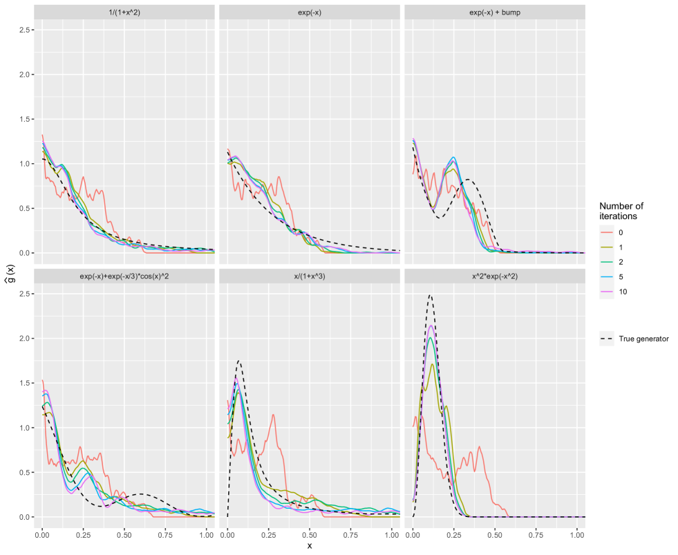
Fig. 2: Estimated generators by the iterative method MECIP, with $n=1000$, $d=2$, $\rho=0.2$, $a=1$, $h=0.05$ and starting point = “identity”.

In Fig. 3, the mean integrated squared error $\text{MISE}(\hat{g}_{h}):=E[||\hat{g}_{h}-g||_{2}^{2}]$ of our iterative estimator is plotted as a function of the bandwidth $h$, for different true generators $g$ and initialization strategies. These MISE are computed using $N$ equal to ten and $100$ replications of each experiment. As expected, a clear-cut optimal bandwidth can be empirically identified for most generators.

Restricting ourselves to the case of the Gaussian generator, we then study the joint influence of the sample size $n$ and of the bandwidth $h$ on the MISE of our estimators, using the “identity” initialization: see Fig. 4. We find the same behaviors as for usual kernel-based estimators: empirically, the optimal bandwidths are ”closely” linear functions of $\ln(n)$. The computation time for the three initialization methods are compared in Fig. 7. They are mostly similar. The “Gaussian” initialization is the fastest method as it is not data-dependent.

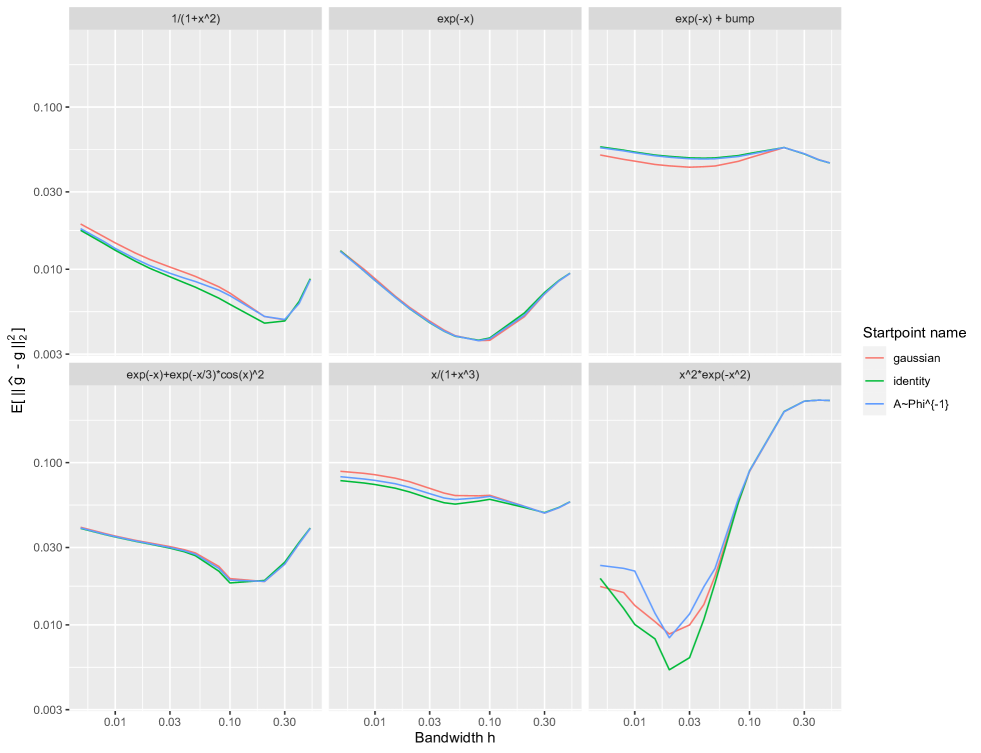
Fig. 3: MISE of the estimates given by Algorithm 2 for $n=1000$, different choices of the generator $g$, the bandwidth $h$ and the initialization method.

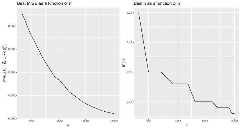
Fig. 4: MISE of the estimate given by Algorithm 2 as a function of $n$, for the best bandwidth $h=h^{*}(n)$, and $h^{*}(n)$ as a function of $n$. Both plots are in semi-log scale. The true generator is the Gaussian $g(x)=e^{-x}$ with the initialization “identity”.

4.2 Simulation study for higher dimensions

Here, we consider the same sample size $n=1000$ as before, but the dimension $d$ varies between $3$ and $11$. The correlation matrix is chosen as $\Sigma_{i,j}=0.2$ when $i\neq j$. For the Gaussian generator, we then study the performance of our algorithm as a function of the tuning parameters $a$ and $h$. The results are displayed in Fig. 5. We observe that the MSE increases with the dimension, even for the best choices of the tuning parameters $a$ and $h$. When $d\geq 5$, avoid choosing $a$ less than one, while the influence of the bandwidth $h$ seems to be less crucial.

Computation times increase only slowly with the dimension $d$: see Fig. 7. This is because the generator is a univariate function regardless the dimension of the random vector. Therefore, most steps in our algorithms are invariant with respect to the dimension $d$, except the transformation of the sample $Y_{i}:=\psi_{a}\big{(}\hat{\bf Z}_{i}^{\top}\,\hat{\bm{\Sigma}}\,\hat{\bf Z}_{i}\big{)}$. The latter step costs at most $(4d^{2}+2d+3)n$ elementary operations, a reasonable amount when $d$ is moderate.

Remark 3.

Actually, it is possible to bypass the problem of high dimensions $d$. Indeed, any subvector of an elliptical distribution is itself elliptically distributed (see Eq. (21) and the related discussion). As a consequence, if the copula of a random vector ${\bf Y}$ is elliptical with generator $g_{d}$, then the copula of a subvector ${\bf Y}_{(m)}$ of $m$ components of ${\bf Y}$ is still an elliptical copula whose generator $g_{m}$ is given by Eq. (21). Therefore, it is possible to estimate the generator of an elliptical copula by using only a sample of $m$-dimensional subvectors. By a numerical inversion of Eq. (21), one would get a generator that corresponds to the copula of the whole vector ${\bf Y}$.

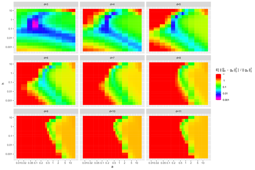
Fig. 5: MISE of the estimate given by Algorithm 2 as a function of $a,h$, for $n=1000$, and different choice of the dimension $d$. The true generator is the Gaussian $g(x)=e^{-x}$ with the initialization “identity”.

Fig. 6: Density plot of the computation time as a function of the starting point, for $d=2$ and $n=1000$.

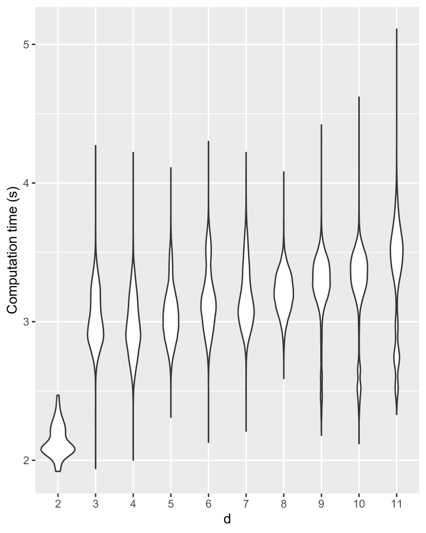
Fig. 7: Density plot of the computation time as a function of the dimension, for the initialization method “identity” and $n=1000$.

4.3 When ${\bm{\Sigma}}$ is non exchangeable and almost non invertible

We consider the same setting as in the previous section, and we aim for measuring the effect of the lack of exchangeability in the matrix ${\bm{\Sigma}}$ on the estimation of $g$. For this, two different frameworks are considered.

1. First framework: the dimension is $d=3$, $h=a=0.2$ and the correlation matrix is ${\bm{\Sigma}}_{(3)}(\rho_{12})=\begin{pmatrix}1&\rho_{12}&0.2\\ \rho_{12}&1&0.2\\ 0.2&0.2&1\end{pmatrix}$.

2. Second framework: the dimension is $d=10$, $a=1$, $h=0.1$ and the correlation matrix is

   $${\bm{\Sigma}}_{(10)}(\rho_{12}):=\begin{pmatrix}1&\rho_{12}&\rho_{12}&0.2&\cdots&0.2\\ \rho_{12}&1&\rho_{12}&0.2&\cdots&0.2\\ \rho_{12}&\rho_{12}&1&0.2&\cdots&0.2\\ 0.2&0.2&0.2&1&\ddots&\vdots\\ \vdots&\vdots&\vdots&\ddots&\ddots&0.2\\ 0.2&0.2&0.2&\cdots&0.2&1\end{pmatrix}$$

Note that there exists a value $\underline{\rho_{12}}$ for which ${\bm{\Sigma}}_{(3)}(\rho_{12})$ and ${\bm{\Sigma}}_{(10)}(\rho_{12})$ are positive semi-definite if and only if $\rho_{12}>\underline{\rho_{12}}$. For the first and the second frameworks, $\underline{\rho_{12}}\approx-0.919$ and $\underline{\rho_{12}}\approx-0.432$ respectively.

The MISE is computed for both frameworks as a function of $\rho_{12}$ and is displayed respectively in Fig. 9 and 9. On these figures, the MISE stays stable whenever $\rho_{12}$ is not too close to the boundary value $\underline{\rho_{12}}$. When $\rho_{12}$ is close to $\underline{\rho_{12}}$, the estimator of the correlation matrix becomes unreliable, degrading the performance of the estimator $\hat{g}$. This deterioration is stronger in the second framework where $d=10$. Note that, as in the previous section, the performance for $d=10$ is always worse than for $d=3$ even far away from the boundary.

Fig. 8: MISE of the estimate given by Algorithm 2 as a function of $\rho_{12}$ for $d=3$ and $n=1000$, where the correlation matrix is ${\bm{\Sigma}}_{(3)}(\rho_{12})$.

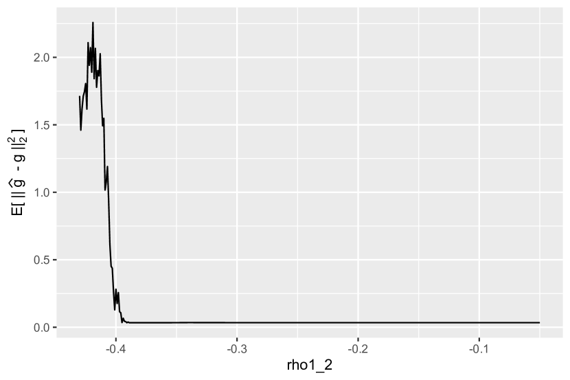
Fig. 9: MISE of the estimate given by Algorithm 2 as a function of $\rho_{12}$ for $d=10$ and $n=1000$, where the correlation matrix is ${\bm{\Sigma}}_{(10)}(\rho_{12})$.

4.4 Simulation study with missing values

In this case, we choose $n=1000$, $d=3$, and the same correlation matrix as before. Contrary to the previous simulation experiments, we introduce some missing values in the dataset (represented by NA in the R environment). The missing values are generated as follows: we fix a number $N_{missing}$ of observations that are affected by missing values; we randomly draw a number $N_{missing,1}$ of observations (uniformly between $0$ and $N_{missing}$) for which a single component is missing; let $N_{missing,2}:=N_{missing}-N_{missing,1}$ be the number of observations for which two components are missing. Because $d=3$, considering the case of three missing components does not make sense because this would induce an empty vector (which should rather induce a smaller sample size rather than a missing value issue if it were the case). We select $N_{missing,1}$ (respectively $N_{missing,2}$) observations at random, and replace the missing values by NA.

For the estimation procedure, we choose $a=0.08$ and $h=0.2$, the optimal choices according to Fig. 5. The corresponding MISE are displayed in Fig. 10. They show that the MISE deteriorates as the number of missing values increases, but this tendency is not very strong.

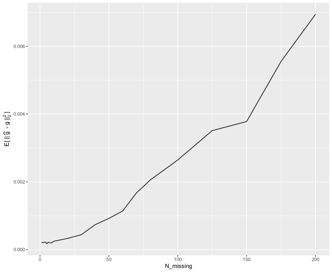
Fig. 10: MISE of the estimate given by Algorithm 2 as a function of the number of observations that contains missing values. The sample size is $n=1000$, the dimension is $d=3$ and the true generator is the Gaussian $g(x)=e^{-x}$ with the initialization “identity”.

5 Conclusion

We have stated some sufficient conditions to obtain the identifiability of the generator $g$ of a meta-elliptical copula. In many standard practical situations, they are satisfied, particularly when the corresponding correlation matrix ${\bm{\Sigma}}$ is not the identity matrix. Some inference procedures have been discussed, in particular an iterative method called MECIP that yields satisfying empirical results.

Among the avenues for further studies, a theoretically sound data-driven bandwidth selector would be welcome. The theoretical properties of the iterative algorithm (consistency, rate of convergence) remains unknown, even if the procedure seems to behave conveniently in our experiments. The proof of such results would be particularly challenging, due to the highly nonlinear analytical features of the maps we use in our algorithm MECIP. Moreover, it would be nice to weaken the conditions for the identifiability of $g$ when ${\bm{\Sigma}}={\bf I}_{d}$ (Proposition 4). Finally, we conjecture that our results apply even when $g(0)=0$, a situation that was excluded for the sake of clarity in the theoretical developments, but that seems to be conveniently managed in our numerical experiments.

Acknowledgements

Jean-David Fermanian has been supported by the labex Ecodec (reference project ANR-11-LABEX-0047).

Appendix A A reminder about elliptical random vectors

Let ${\bf X}$ be a $d$-dimensional elliptical random vector, ${\bf X}\sim\mbox{$\mathcal{E}$}_{d}({\bm{\mu}},{\bm{\Omega}},g_{d})$. When there is no ambiguity, $g_{d}$ will simply be denoted $g$. We recall a key representation of any elliptical random vector ${\bf X}$ in $\mbox{$\mathbb{R}$}^{d}$, that can be considered as a definition.

Definition 1 (polar decomposition).

A random vector ${\bf X}$ follows an elliptical distribution $\mbox{$\mathcal{E}$}_{d}({\bm{\mu}},{\bm{\Omega}},g)$ if ${\bf X}\buildrel{d}\over{=}{{\bm{\mu}}+R{\bf A}^{\top}{\bf V}}$, for some $d\times d$ matrix ${\bf A}$ such that ${\bf A}^{\top}{\bf A}={\bm{\Omega}}$, where ${\bf V}$ is a random vector uniformly distributed on the $d$-dimensional unit sphere and $R$ is a nonnegative r.v. independent of ${\bf V}$. When $R$ has a density $g_{R}$ with respect to the Lebesgue measure on $\mbox{$\mathbb{R}$}^{+}$ and no mass at zero, this is the case for ${\bf X}$ too. The density $f_{{\bf X}}$ of ${\bf X}$ is then given by

$$f_{{\bf X}}({\bf x})={|{\bm{\Omega}}|}^{-1/2}g\left(({\bf x}-{\bm{\mu}})^{\top}\,{\bm{\Omega}}^{-1}\,({\bf x}-{\bm{\mu}})\right),\;{\bf x}\in\mbox{$\mathbb{R}$}^{d},$$

and we have

$$g_{R}(r)=s_{d}r^{d-1}g(r^{2}),\;r\geq 0.$$ (20)

See [21], Theorem 3, and [7], Section 4. We denote by ${\bf X}\sim\tilde{}\mbox{$\mathcal{E}$}_{d}({\bm{\mu}},{\bf A},g_{R})$ the latter “polar decomposition”. It is said that $R$ is the modular variable of ${\bf X}$, and its density $g_{R}$ is the associated modular density. In our paper, we assume that ${\bf X}$ has a density $f_{{\bf X}}$ with respect to the Lebesgue measure on $\mbox{$\mathbb{R}$}^{d}$. The support of $f_{{\bf X}}$ is $\{{\bf x};\sum_{j=1}^{d}x_{j}^{2}<M\}$ for some $M\in\bar{}\mbox{$\mathbb{R}$}^{+}$ ([27], p.422).

The associated vector ${\bf Y}={\bm{\Omega}}^{-1/2}({\bf X}-{\bm{\mu}})$ is spherical, ${\bf Y}\sim\mbox{$\mathcal{E}$}_{d}({\mathbf{0}},{\bf I}_{d},g_{d})$. It is well-known that sub-vectors of ${\bf X}$ (resp. ${\bf Y}$) are elliptical (resp. spherical) too: see Theorem 6 of Gomez et al. [21] (density generator), Embrechts et al. (p.10) [10] (characteristic generator), Theorem 1 of Kano [26], among others. See the recent surveys [2, 39] about elliptical and meta-elliptical distributions.

Actually, our two parameterizations of elliptical distributions above are essentially unique.

Proposition 6.

Let ${\bf X}$ be a $d$-dimensional random vector.

• If ${\bf X}\sim\tilde{}\mbox{$\mathcal{E}$}_{d}({\bm{\mu}}_{1},{\bf A}_{1},g_{R}^{(1)})$ and ${\bf X}\sim\tilde{}\mbox{$\mathcal{E}$}_{d}({\bm{\mu}}_{2},{\bf A}_{2},g_{R}^{(2)})$, then there exists a constant $a>0$ such that ${\bm{\mu}}_{1}={\bm{\mu}}_{2}$, ${\bf A}_{1}^{\top}{\bf A}_{1}=a{\bf A}_{2}^{\top}{\bf A}_{2}$, $R_{1}\buildrel{d}\over{=}{a^{-1/2}R_{2}}$, $g_{R}^{(1)}(t)=\sqrt{a}\,g_{R}^{(2)}(t\sqrt{a}),$ for almost every $t$.

• If ${\bf X}\sim\mbox{$\mathcal{E}$}_{d}({\bm{\mu}}_{1},{\bm{\Omega}}_{1},g^{(1)})$ and ${\bf X}\sim\mbox{$\mathcal{E}$}_{d}({\bm{\mu}}_{2},{\bm{\Omega}}_{2},g^{(2)})$, then there exists a constant $a>0$ such that ${\bm{\mu}}_{1}={\bm{\mu}}_{2}$, ${\bm{\Omega}}_{1}=a{\bm{\Omega}}_{2}$, and $g^{(1)}(t)=a^{d/2}g^{(2)}(at),$ for almost every $t$.

Proof of Proposition 6.

Point $(a)$ is a consequence of Theorem 3 (ii) in [7]. The proof of point $(b)$ is deduced from Proposition 1: for $k\in\{1,2\}$, there exists $({\bf A}_{k},g_{R^{(k)}})$ such that $\mbox{$\mathcal{E}$}_{d}({\bm{\mu}}_{k},{\bm{\Omega}}_{k},g^{(k)})\buildrel{d}\over{=}\tilde{}\mbox{$\mathcal{E}$}_{d}({\bm{\mu}}_{k},{\bf A}_{k},g_{R}^{(k)})$, and then apply point $(a)$. In particular, applying Eq. (20) twice, we get

$$s_{d}t^{(d-1)/2}g^{(1)}(t)=g_{R}^{(1)}(\sqrt{t})=\sqrt{a}g_{R}^{(2)}(\sqrt{at})=s_{d}(at)^{(d-1)/2}\sqrt{a}g^{(2)}(at),$$

for every $t$, proving the asserted relationship between $g^{(1)}$ and $g^{(2)}$. ∎

As a consequence, in order to get unique sets of ${\bf X}$-parameters, it is necessary to impose an additional identification constraint. Obviously, ${\bm{\mu}}=E[{\bf X}]$ is uniquely defined. Moreover, due to Proposition 6, ${\bm{\Omega}}$ (resp. ${\bf A}$) is defined up to a positive constant. Typically, when ${\bf X}$ has finite second moments, it is natural to impose $\text{Cov}({\bf X})={\bm{\Omega}}={\bf A}^{\top}{\bf A}$. Otherwise, it is still possible to impose $\text{Tr}({\bm{\Omega}})=1$ or other similar constraints. Once ${\bm{\Omega}}$ is uniquely defined, this will be the case for $g$, as deduced from Proposition 6. In other words, the usual constraint

$$s_{d}\int_{0}^{\infty}r^{d-1}g(r^{2})\,dr=s_{d}\int_{0}^{\infty}t^{d/2-1}g(t)\,dt/2=1,$$

where $s_{d}:=2\pi^{d/2}/\Gamma(d/2)$ plus a single additional constraint imply the identifiability of the law of any elliptically distributed random vector.

Let us specify how subvectors of an elliptically distributed vector are still elliptical, recalling Cambanis et al. [7] (Section 4) or [14] (Eq. (2.23)): if ${\bf Y}\sim\mbox{$\mathcal{E}$}_{d}({\mathbf{0}},{\bf I}_{d},g_{d})$, then the subvector ${\bf Y}_{(m)}$ of the first $m$ components of ${\bf Y}_{(d)}$, $m<d$ is still spherical, i.e., ${\bf Y}_{(m)}\sim\mbox{$\mathcal{E}$}_{m}({\mathbf{0}},{\bf I}_{m},g_{m})$, where

$$g_{m}(u)=s_{n-m}\int_{0}^{\infty}g_{d}(u+r^{2})r^{d-m-1}\,dr,$$ (21)

where $s_{k}$ denotes the surface of the $k$-dimensional unit sphere in $\mbox{$\mathbb{R}$}^{d}$, i.e., $s_{k}=2\pi^{k/2}/\Gamma(k/2)$, $k\geq 1$. We deduce

$$g_{1}(u)=\frac{\pi^{(d-1)/2}}{\Gamma((d-1)/2)}\int_{0}^{\infty}g_{d}(u+s)s^{(d-3)/2}\,ds.$$ (22)

Note that $X_{k}\sim\mbox{$\mathcal{E}$}(0,\Omega_{kk},g_{1})$ for any $k\in\{1,\ldots,d\}$, where ${\bm{\Omega}}=:[\Omega_{k,l}]$ and $g_{1}$ as above ([21], Th. 6). Therefore, its density is $f_{k}(t)=g_{1}(t^{2}/\Omega_{kk})/\sqrt{\Omega_{kk}}$ for every real $t$. When $\Omega_{kk}=1$, as in the case of correlation matrices ${\bm{\Omega}}$, the density of any margin of $\mbox{$\mathcal{E}$}_{d}({\mathbf{0}},{\bm{\Omega}},g)$ is

$$f_{g}(t):=g_{1}(t^{2})=\frac{s_{d-1}}{2}\int_{0}^{\infty}g(t^{2}+s)s^{(d-3)/2}\,ds=s_{d-1}\int_{0}^{\infty}g(t^{2}+r^{2})r^{d-2}\,dr.$$ (23)

Clearly, $f_{g}$ is even. Denote by $a_{g}^{2}\in\bar{}\mbox{$\mathbb{R}$}^{+}$ the upper bound of $g$’s support (possibly equal to $+\infty$). Then, it is easy to see that the support of $f_{g}$ is $(-a_{g},a_{g})$, possibly including its boundaries. When $g$ is bounded in a neighborhood of a positive real number $t$, then $g_{1}$ is continuous at $t$ too ([27], Lemma 3). As a consequence, $f_{g}$ is continuous at $\pm\sqrt{t}$. Finally, Theorem 6 in Gomez et al. [21] provides similar relationships in terms of modular variables.

Let us discuss the nonparametric inference of density generators. Assume we observe an i.i.d. sample $({\bf X}_{1},\ldots,{\bf X}_{n})$ drawn along ${\bf X}\sim\mbox{$\mathcal{E}$}_{d}({\bm{\mu}},{\bm{\Sigma}},g)$ for some correlation matrix ${\bm{\Sigma}}$. The statistical estimation of the underlying parameters has been studied in the literature. First, it is easy to evaluate ${\bm{\mu}}$ by $\hat{\bm{\mu}}$, the empirical mean of the vectors ${\bf X}_{i}$, $i\in\{1,\ldots,n\}$. Second, an estimator $\hat{\bm{\Sigma}}$ of ${\bm{\Sigma}}$ can be obtained by empirical Kendall’s taus’. Now, set the standardized vector ${\bf Y}:={\bm{\Sigma}}^{-1/2}\,({\bf X}-{\bm{\mu}})$, and the standardized observations $\hat{\bf Y}_{i}:=\hat{\bm{\Sigma}}^{-1/2}\,({\bf X}_{i}-\hat{\bm{\mu}})$, $i\in\{1,\ldots,n\}$. Note that the latter observations are identically distributed but not independent.

Third, we know that the law of ${\bf Y}$ is spherical, ${\bf Y}\sim\mbox{$\mathcal{E}$}_{d}({\mathbf{0}},{\bf I}_{d},g)$, and depends on $g$ only. The task of estimating $g$ is relatively challenging and a few techniques have been proposed in the literature. In Battey and Linton [3], the estimation of the density generator is done by a finite mixture sieve. Bhattacharyya [5] proposed piecewise constant estimators of $g$, that are fitted by log-linear splines. In [6], they also provided an EM-algorithm to estimate the parameters of elliptical distributions mixtures. Stute and Werner [47] introduced a usual kernel density estimator of $\|{\bf Y}\|^{2}$’s law. Since $\|{\bf Y}\|^{2}=R^{2}$ through the polar decomposition of ${\bf X}$, and invoking (20), they deduced the following estimator of the ${\bf Y}$ density:

$$f_{n}({\bf y})=\frac{2}{s_{d}\,n\,h_{n}\,{||{\bf y}||}^{d-2}}\sum_{i=1}^{n}K\left(\frac{{||{\bf y}||}^{2}-{||\hat{\bf Y}_{i}||}^{2}}{h_{n}}\right),\;{\bf y}\in\mbox{$\mathbb{R}$}^{d},$$ (24)

for a bandwidth $h_{n}>0$ and a one-dimensional kernel $K(\cdot)$. Since $f_{Y}({\bf y})=g(\|{\bf y}\|^{2})$, an estimate of the density generator $g$ itself is

$$\hat{g}(u)=\frac{2}{s_{d}n\,h_{n}\,u^{(d-2)/2}}\sum_{i=1}^{n}K\left(\frac{u-{||\hat{\bf Y}_{i}||}^{2}}{h_{n}}\right),\;u\in\mbox{$\mathbb{R}$}^{+}.$$ (25)

These ideas have been refined by Liebscher [33] and applied by [40], notably. He noticed that the estimator (25) does not behave conveniently close to the origin. He proposed to nonlinearly transform the data before invoking a kernel estimator, to avoid convergence problems in boundary regions.

Appendix B Finite distance properties of $\hat{\theta}_{n,m}$

To this end, introduce the pseudo-true value of the parameter $\theta_{m}^{*}$. It is the “best” value of the parameter when the model is assumed to belong to ${\mathcal{G}}_{m}$: generally speaking, for a divergence $D(\cdot,\cdot)$ between distributions on $\mbox{$\mathbb{R}$}^{d}$, define

$$\theta_{m}^{*}:=\underset{\theta:\,g_{\theta}\in{\mathcal{G}}_{m}}{\arg\min}\,D\big{(}{\mathbb{P}}_{0},{\mathbb{P}}_{g_{\theta},{\bm{\Sigma}},F_{1},\ldots,F_{d}}\big{)},$$ (26)

where ${\mathbb{P}}_{0}$ is the law of the observations (the true DGP) and ${\mathbb{P}}_{\bar{g},\bar{\bm{\Sigma}},\bar{F}_{1},\ldots,\bar{F}_{d}}$ is the law induced by a Trans-elliptical distribution $\mbox{$\mathcal{T}$}\mbox{$\mathcal{E}$}_{d}(\bar{g},\bar{\bm{\Sigma}},\bar{F}_{1},\ldots,\bar{F}_{d})$. Here, we set

$$D\big{(}{\mathbb{P}}_{0},{\mathbb{P}}_{g_{\theta},{\bm{\Sigma}},F_{1},\ldots,F_{d}}\big{)}:=E\big{[}{\mathbb{G}}_{n}(\theta,\mbox{$\mathcal{U}$})\big{]},$$

and we assume $\theta_{m}^{*}$ satisfies the first-order condition $E\big{[}\nabla_{\theta}{\mathbb{G}}_{n}(\theta_{m}^{*},\mbox{$\mathcal{U}$})\big{]}=0$.

Condition 3.

The pseudo-true parameters are “sparse”: $card(\mbox{$\mathcal{A}$}_{m})=k_{m}<p_{m}$ and $\mbox{$\mathcal{A}$}_{m}=\{i:\theta^{*}_{m,i}\neq 0\}$.

Condition 4.

We consider coordinate-separable penalty (or regularizer) functions $\mbox{\boldmath$p$}_{n}:\mbox{$\mathbb{R}$}_{+}\times\mbox{$\mathbb{R}$}^{p_{n}}\rightarrow\mbox{$\mathbb{R}$}$, i.e., $\mbox{\boldmath$p$}_{n}(\lambda_{n},\theta)=\overset{p_{n}}{\underset{k=1}{\sum}}p(\lambda_{n},\theta_{k})$. Moreover, for some $\mu\geq 0$, the regularizer $\mbox{\boldmath$p$}_{n}(\lambda_{n},\cdot)$ is assumed to be $\mu$-amenable, in the sense that

• $\rho\mapsto p(\lambda_{n},\rho)$ is symmetric around zero and $p_{n}(\lambda_{n},0)=0$.

• $\rho\mapsto p(\lambda_{n},\rho)$ is non-decreasing on $\mbox{$\mathbb{R}$}_{+}$.

• $\rho\mapsto p(\lambda_{n},\rho)/\rho$ is non-increasing on $\mbox{$\mathbb{R}$}_{+}\setminus\{0\}$.

• $\rho\mapsto p(\lambda_{n},\rho)$ is differentiable for any $\rho\neq 0$.

• $\underset{\rho\rightarrow 0^{+}}{\lim}p^{\prime}(\lambda_{n},\rho)=\lambda_{n}$.

• $\rho\mapsto p(\lambda_{n},\rho)+\mu\rho^{2}/2$ is convex for some $\mu\geq 0$.
  The regularizer $\mbox{\boldmath$p$}_{n}(\lambda_{n},.)$ is said $(\mu,\gamma)$-amenable if, in addition,

• There exists $\gamma\in(0,\infty)$ such that $p^{\prime}(\lambda_{n},\rho)=0$ for $\rho\geq\lambda_{n}\gamma$.

The latter assumption provides regularity conditions to potentially manage non-convex penalty functions. These regularity conditions are the same as in [36, 38, 37]. Some usual penalties are the Lasso, the SCAD ([11]) and the MCP ([53]), given by

$$\begin{array}[]{llll}\mathbf{Lasso:}\;\;p(\lambda_{n},\rho)&=&\lambda_{n}|\rho|,\\ \mathbf{MCP:}\;\;p(\lambda_{n},\rho)&=&sign(\rho)\lambda_{n}\int^{|\rho|}_{0}\{1-z/(\lambda_{n}b_{mcp})\}_{+}dz,\\ \mathbf{SCAD:}\;\;p(\lambda_{n},\rho)&=&\begin{cases}\lambda_{n}|\rho|,&\text{for}\;\;|\rho|\leq\lambda_{n},\\ -(\rho^{2}-2b_{scad}\lambda_{n}|\rho|+\lambda^{2}_{n})/\{2(b_{scad}-1)\},&\text{for}\;\;\lambda_{n}\leq|\rho|\leq b_{scad}\lambda_{n},\\ (b_{scad}+1)\lambda^{2}_{n}/2,&\text{for}\;\;|\rho|>b_{scad}\lambda_{n},\end{cases}\end{array}$$

where $b_{scad}>2$ and $b_{mcp}>0$ are fixed parameters for the SCAD and MCP respectively. The Lasso is a $\mu$-amenable regularizer, whereas the SCAD and the MCP regularizers are $(\mu,\gamma)$-amenable. More precisely, $\mu$ is equal to zero, $1/(b_{scad}-1)$ or $1/b_{mcp}$ for the Lasso, SCAD or MCP respectively.

As for many parametric models, numerous empirical log-likelihoods associated to copulas are not concave functions in their parameters, at finite distance and globally on $\Theta_{m}$. Moreover, this is still the case for some popular regularizers, as SCAD. The restricted strong convexity is a key ingredient that allows the management of non-convex loss functions. Intuitively, we would like to handle a loss function that locally admits some curvature around its optimum. The latter one can be due to the discrepancy between the empirical loss and the “true” loss, to a non-convex penalty or even to the use of pseudo-observations instead of usual ones.

We say that an empirical loss function ${\mathbb{L}}_{n}$ satisfies the restricted strong convexity condition (RSC) at $\theta$ if there exist two positive functions $\alpha_{1},\alpha_{2}$ and two nonnegative functions $\nu_{1},\nu_{2}$ of $(\theta,n,d)$ such that, for any $\Delta\in\mbox{$\mathbb{R}$}^{d}$,

$$\langle\nabla_{\theta}{\mathbb{L}}_{n}(\theta+\Delta)-\nabla_{\theta}{\mathbb{L}}_{n}(\theta),\Delta\rangle \geq \alpha_{1}\|\Delta\|^{2}_{2}-\nu_{1}\|\Delta\|^{2}_{1},\;\text{if }\|\Delta\|_{2}\leq 1,$$

$$\langle\nabla_{\theta}{\mathbb{L}}_{n}(\theta+\Delta)-\nabla_{\theta}{\mathbb{L}}_{n}(\theta),\Delta\rangle \geq \alpha_{2}\|\Delta\|_{2}-\nu_{2}\|\Delta\|_{1},\;\text{if }\|\Delta\|_{2}>1.$$

Note that the (RSC) property is fundamentally local and that $\alpha_{k},\nu_{k}$, $k\in\{1,2\}$ depend on the chosen $\theta$. To weaken notations, we simply write $\alpha_{k}$ and $\nu_{k}$, $k\in\{1,2\}$, by skipping their implicit arguments $(\theta,n,d)$.

Theorem 7 (Poignard and Fermanian, 2021).

Suppose the objective function ${\mathbb{G}}_{n}(\cdot,\widehat{}\mbox{$\mathcal{U}$}):\Theta_{m}\subset\mbox{$\mathbb{R}$}^{p_{m}}\rightarrow\mbox{$\mathbb{R}$}$ satisfies the (RSC) condition at $\theta_{m}^{*}$. Moreover, $\mbox{\boldmath$p$}(\lambda_{n},\cdot)$ is assumed to be $\mu$-amenable, with $3\mu<4\alpha_{1}$ and $4R\nu_{2}\leq\alpha_{2}$. Assume

$$4\max\Big{\{}\|\nabla_{\theta}{\mathbb{G}}_{n}(\theta_{m}^{*},\widehat{}\mbox{$\mathcal{U}$})\|_{\infty},2R\nu_{1}\Big{\}}\leq\lambda_{n}\leq\cfrac{\alpha_{2}}{6R}\cdot$$ (27)

Then, for every $n$, any stationary point $\hat{\theta}_{n,m}$ of (16) satisfies

$$\|\hat{\theta}_{n,m}-\theta_{m}^{*}\|_{2}\leq\cfrac{6\lambda_{n}\sqrt{k_{m}}}{4\alpha_{1}-3\mu},\;\text{and}\;\;\|\hat{\theta}_{n,m}-\theta_{m}^{*}\|_{1}\leq\cfrac{6(16\alpha_{1}-9\mu)}{(4\alpha_{1}-3\mu)^{2}}\lambda_{n}k_{m}.$$

The proof straightforward extends Theorem 1 in [41]. In particular, if the “true” generator $g$ of the data belongs to some subset ${\mathcal{G}}_{m_{0}}$ (the model is correctly specified from the index $m_{0}$ on), then $\theta_{m_{0}}^{*}=\theta_{0}$. When we work with true realizations of ${\bf U}$, a typical behavior is $\lambda_{n}\asymp(\ln p_{n}/n)^{1/2}$ (see [36]). As discussed in [41], this rate is getting worse in general when dealing with pseudo-observations in $\widehat{}\mbox{$\mathcal{U}$}$: $\lambda_{n}$ will be at most of order $dp_{n}^{2}/\sqrt{n}$.

References

- Abdous et al. [2005] B. Abdous, C. Genest, B. Rémillard, Dependence properties of meta-elliptical distributions, in: Statistical modeling and analysis for complex data problems, Springer, 2005, pp. 1–15.
- Babić et al. [2019] S. Babić, C. Ley, D. Veredas, Comparison and classification of flexible distributions for multivariate skew and heavy-tailed data, Symmetry 11 (2019) 1216.
- Battey and Linton [2014] H. Battey, O. Linton, Nonparametric estimation of multivariate elliptic densities via finite mixture sieves, Journal of Multivariate Analysis 123 (2014) 43–67.
- Berghaus et al. [2017] B. Berghaus, A. Bücher, S. Volgushev, Weak convergence of the empirical copula process with respect to weighted metrics, Bernoulli 23 (2017) 743–772.
- Bhattacharyya [2013] S. Bhattacharyya, A Study of High-dimensional Clustering and Statistical Inference of Networks, Ph.D. thesis, University of California, Berkeley, 2013.
- Bhattacharyya and Bickel [2014] S. Bhattacharyya, P. J. Bickel, Adaptive estimation in elliptical distributions with extensions to high dimensions, Preprint, 2014.
- Cambanis et al. [1981] S. Cambanis, S. Huang, G. Simons, On the theory of elliptically contoured distributions, Journal of Multivariate Analysis 11 (1981) 368–385.
- Chen [2007] X. Chen, Large sample sieve estimation of semi-nonparametric models, Handbook of Econometrics 6 (2007) 5549–5632.
- Derumigny and Fermanian [2022] A. Derumigny, J.-D. Fermanian, R package: ElliptCopulas, version 0.1.1, Available at https://cran.r-project.org/package=ElliptCopulas, 2022.
- Embrechts et al. [2002] P. Embrechts, A. McNeil, D. Straumann, Correlation and dependence in risk management: properties and pitfalls, Risk Management: Value at Risk and Beyond (2002) 176–223.
- Fan and Li [2001] J. Fan, R. Li, Variable selection via nonconcave penalized likelihood and its oracle properties, Journal of the American Statistical Association 96 (2001) 1348–1360.
- Fan and Peng [2004] J. Fan, H. Peng, Nonconcave penalized likelihood with a diverging number of parameters, The Annals of Statistics 32 (2004) 928–961.
- Fang et al. [2002] H.-B. Fang, K.-T. Fang, S. Kotz, The meta-elliptical distributions with given marginals, Journal of Multivariate Analysis 82 (2002) 1–16.
- Fang et al. [1990] K.-T. Fang, S. Kotz, K.-W. Ng, Symmetric Multivariate and Related Distributions, Springer, New-York, 1990.
- Fermanian et al. [2004] J.-D. Fermanian, D. Radulovic, M. Wegkamp, Weak convergence of empirical copula processes, Bernoulli 10 (2004) 847–860.
- Frahm et al. [2003] G. Frahm, M. Junker, A. Szimayer, Elliptical copulas: applicability and limitations, Statistics & Probability Letters 63 (2003) 275–286.
- Genest et al. [2007] C. Genest, A.-C. Favre, J. Béliveau, C. Jacques, Metaelliptical copulas and their use in frequency analysis of multivariate hydrological data, Water Resources Research 43 (2007).
- Genest et al. [1995] C. Genest, K. Ghoudi, L.-P. Rivest, A semiparametric estimation procedure of dependence parameters in multivariate families of distributions, Biometrika 82 (1995) 543–552.
- Ghoudi and Rémillard [1998] K. Ghoudi, B. Rémillard, Empirical processes based on pseudo-observations, in: Asymptotic Methods in Probability and Statistics, Elsevier, 1998, pp. 171–197.
- Ghoudi and Rémillard [2004] K. Ghoudi, B. Rémillard, Empirical processes based on pseudo-observations II: the multivariate case, Fields Inst. Commun 44 (2004) 381–406.
- Gómez et al. [2003] E. Gómez, M. A. Gómez-Villegas, J. M. Marín, A survey on continuous elliptical vector distributions, Revista Matemática Complutense 16 (2003) 345–361.
- Higham [2002] N. J. Higham, Computing the nearest correlation matrix—a problem from finance, IMA journal of Numerical Analysis 22 (2002) 329–343.
- Higham et al. [2016] N. J. Higham, N. Strabic, V. Sego, Restoring definiteness via shrinking, with an application to correlation matrices with a fixed block, SIAM Review 58 (2016) 245–263.
- Jaser et al. [2017] M. Jaser, S. Haug, A. Min, A simple non-parametric goodness-of-fit test for elliptical copulas, Dependence Modeling 5 (2017) 330–353.
- Jaser and Min [2020] M. Jaser, A. Min, On tests for symmetry and radial symmetry of bivariate copulas towards testing for ellipticity, Computational Statistics (2020) 1–26.
- Kano [1994] Y. Kano, Consistency property of elliptic probability density functions, Journal of Multivariate Analysis 51 (1994) 139–147.
- Kelker [1970] D. Kelker, Distribution theory of spherical distributions and a location-scale parameter generalization, Sankhyā: The Indian Journal of Statistics, Series A (1970) 419–430.
- Klüppelberg et al. [2007] C. Klüppelberg, G. Kuhn, L. Peng, Estimating the tail dependence function of an elliptical distribution, Bernoulli 13 (2007) 229–251.
- Klüppelberg et al. [2008] C. Klüppelberg, G. Kuhn, L. Peng, Semi-parametric models for the multivariate tail dependence function–the asymptotically dependent case, Scandinavian Journal of Statistics 35 (2008) 701–718.
- Kostadinov [2005] K. Kostadinov, Non-parametric estimation of elliptical copulae with application to credit risk, Preprint, 2005.
- Kurowicka et al. [2000] D. Kurowicka, J. Misiewicz, R. Cooke, Elliptical copulae, in: Proc of the International Conference on Monte Carlo Simulation-Monte Carlo, pp. 209–214.
- Levasseur [1984] K. M. Levasseur, A probabilistic proof of the Weierstrass approximation theorem, The American Mathematical Monthly 91 (1984) 249–250.
- Liebscher [2005] E. Liebscher, A semiparametric density estimator based on elliptical distributions, Journal of Multivariate Analysis 92 (2005) 205–225.
- Liu et al. [2012] H. Liu, F. Han, C.-h. Zhang, Transelliptical graphical models, in: Advances in Neural Information Processing Systems, pp. 809–817.
- Liu et al. [2016] H. Liu, J. Mulvey, T. Zhao, A semiparametric graphical modelling approach for large-scale equity selection, Quantitative Finance 16 (2016) 1053–1067.
- Loh [2017] P.-L. Loh, Statistical consistency and asymptotic normality for high-dimensional robust -estimators, The Annals of Statistics 45 (2017) 866–896.
- Loh and Wainwright [2015] P.-L. Loh, M. J. Wainwright, Regularized m-estimators with nonconvexity: Statistical and algorithmic theory for local optima, The Journal of Machine Learning Research 16 (2015) 559–616.
- Loh and Wainwright [2017] P.-L. Loh, M. J. Wainwright, Support recovery without incoherence: A case for nonconvex regularization, The Annals of Statistics 45 (2017) 2455–2482.
- Paindaveine [2014] D. Paindaveine, Elliptical symmetry, Wiley StatsRef: Statistics Reference Online (2014).
- Pimenova [2012] I. Pimenova, Semi-parametric estimation of elliptical distribution in case of high dimensionality, Master’s thesis, Humboldt-Universität zu Berlin, Wirtschaftswissenschaftliche Fakultät, 2012.
- Poignard and Fermanian [2021] B. Poignard, J.-D. Fermanian, The finite sample properties of sparse m-estimators with pseudo-observations, Annals of the Institute of Statistical Mathematics (2021) 1–31.
- Qi and Sun [2006] H. Qi, D. Sun, A quadratically convergent newton method for computing the nearest correlation matrix, SIAM journal on matrix analysis and applications 28 (2006) 360–385.
- Remillard [2013] B. Remillard, Statistical methods for financial engineering, CRC press, 2013.
- Sancetta and Nikandrova [2009] A. Sancetta, A. Nikandrova, Forecasting and prequential validation for time varying meta-elliptical distributions, Journal of Time Series Econometrics 1 (2009) 1–41.
- Shih and Louis [1995] J. H. Shih, T. A. Louis, Inferences on the association parameter in copula models for bivariate survival data, Biometrics (1995) 1384–1399.
- Song and Singh [2010] S. Song, V. P. Singh, Meta-elliptical copulas for drought frequency analysis of periodic hydrologic data, Stochastic Environmental Research and Risk Assessment 24 (2010) 425–444.
- Stute and Werner [1991] W. Stute, U. Werner, Nonparametric estimation of elliptically contoured densities, in: Nonparametric Functional Estimation and Related Topics, Springer, 1991, pp. 173–190.
- Touboul [2011] J. Touboul, Goodness-of-fit tests for elliptical and independent copulas through projection pursuit, Algorithms 4 (2011) 87–114.
- Tsukahara [2005] H. Tsukahara, Semiparametric estimation in copula models, Canadian Journal of Statistics 33 (2005) 357–375.
- Tsukahara [2011] H. Tsukahara, Erratum to ”Semiparametric estimation in copula models”, Canadian Journal of Statistics 39 (2011) 734–735.
- Wang and Yan [2013] X. Wang, J. Yan, Practical notes on multivariate modeling based on elliptical copulas, Journal de la Société Française de Statistique 154 (2013) 102–115.
- Wegkamp and Zhao [2016] M. Wegkamp, Y. Zhao, Adaptive estimation of the copula correlation matrix for semiparametric elliptical copulas, Bernoulli 22 (2016) 1184–1226.
- Zhang [2010] C.-H. Zhang, Nearly unbiased variable selection under minimax concave penalty, The Annals of Statistics 38 (2010) 894–942.
- Zhao and Genest [2019] Y. Zhao, C. Genest, Inference for elliptical copula multivariate response regression models, Electronic Journal of Statistics 13 (2019) 911–984.