Construction of explicit symplectic integrators in general relativity. IV. Kerr black holes

Abstract

In previous papers, explicit symplectic integrators were designed for nonrotating black holes, such as a Schwarzschild black hole. However, they fail to work in the Kerr spacetime because not all variables can be separable, or not all splitting parts have analytical solutions as explicit functions of proper time. To cope with this difficulty, we introduce a time transformation function to the Hamiltonian of Kerr geometry so as to obtain a time-transformed Hamiltonian consisting of five splitting parts, whose analytical solutions are explicit functions of the new coordinate time. The chosen time transformation function can cause time steps to be adaptive, but it is mainly used to implement the desired splitting of the time-transformed Hamiltonian. In this manner, new explicit symplectic algorithms are easily available. Unlike Runge–Kutta integrators, the newly proposed algorithms exhibit good long-term behavior in the conservation of Hamiltonian quantities when appropriate fixed coordinate time steps are considered. They are better than same-order implicit and explicit mixed symplectic algorithms and extended phase-space explicit symplectic-like methods in computational efficiency. The proposed idea on the construction of explicit symplectic integrators is suitable for not only the Kerr metric but also many other relativistic problems, such as a Kerr black hole immersed in a magnetic field, a Kerr-Newman black hole with an external magnetic field, axially symmetric core-shell systems, and five-dimensional black ring metrics.

Unified Astronomy Thesaurus concepts: Black hole physics (159); Computational methods (1965); Computational astronomy (293); Celestial mechanics (211)

1 Introduction

Gravitational waves and black holes are two fundamental predictions of the theory of general relativity of Einstein. The predictions have been frequently confirmed by a number of observations of gravitational waves from binary black hole or neutron star mergers [e.g., GW150914 (Abbott et al. 2016) and GW190521 (Abbott et al. 2020)] and images of the supermassive black hole candidate in the center of the giant elliptical galaxy M87 (EHT Collaboration et al. 2019). The observed image provides powerful evidence for the presence of a rotating black hole, which was derived by Kerr (1963) from the field equations of general relativity. There are also other solutions for the field equations, such as a non-rotating Schwarzschild black hole.

The geodesics of the Schwarzschild, Reissner-Nordström, Reissner-Nordström-(anti)-de Sitter and Kerr spacetime geometries are highly nonlinear but are integrable. This integrability does not mean that their solutions can be expressed in terms of elementary functions but quadratures. Thus, numerical integration schemes are still necessarily used to solve these geodesic equations. The popular fourth-order Runge-Kutta explicit integration method (RK4) is applicable for arbitrary metrics (i.e., arbitrary spacetimes in arbitrary coordinates). Recently, the RAPTOR code with RK4 was applied to study accretion models of supermassive Kerr black holes so as to produce physically accurate images of black-hole accretion disks (Bronzwaer et al. 2018, 2020). The RK4 integrator is an accurate and efficient integrator for a short integration time. However, it would yield a secular drift in energy errors and would provide unreliable numerical results for a long-term integration. The manifold correction of Nacozy (1971) and its extensions (Fukushima 2003; Wu et al. 2007; Ma et al. 2008; Wang et al. 2016; Wang et al. 2018; Deng et al. 2020) are helpful to compensate for the defect of RK4 by pulling the integrated orbit back to the original integral hypersurface.

The RK4 integrator combined with a manifold correction scheme is regarded as one of the geometric integration algorithms that preserve structures, integrals, symmetries, reversing symmetries, and phase-space volumes (Hairer et al. 1999). The manifold correction scheme can strictly satisfy energy integral, but does not conserve the symplecticity. A class of discrete Hamiltonian gradient schemes that conserve energy to machine precision can be used for any globally hyperbolic spacetimes with six dimensions (Bacchini et al. 2018, 2019), and eight- and ten-dimensional Hamiltonian problems (Hu et al. 2019, 2021). These energy-conserving discrete gradient integrators are implicit, nonsymplectic, and do not preserve other integrals in general. Their constructions become complex as the dimensionality increases. No higher-order accuracy but only first- and second-order accuracies can be given to numerical solutions in the existing energy-conserving discrete gradient schemes.

Symplectic integrators (Swope et al. 1982; Wisdom 1982; Ruth 1983; Forest $\&$ Ruth 1990; Wisdom $\&$ Holman 1991; Chambers $\&$ Murison 2000; Laskar $\&$ Robutel 2001; Omelyan et al. 2003) are the best geometric integrators for studying the long-term evolution of the geodesics and other Hamiltonian problems. Although they are different from the manifold correction schemes and energy-conserving integrators that can exactly preserve energy integral, they remain bounded and show no secular growth in energy errors. Other constants of motion and symplectic geometrical structure are also conserved in the course of numerical integrations. Because of the difficulty of the separation of variables in curved spacetimes, the standard explicit symplectic integrators become useless. Instead, implicit symplectic methods (Feng 1986; Brown 2006; Tsang et al. 2015), or implicit and explicit mixed symplectic methods (Preto $\&$ Saha 2009; Kopáček et al. 2010; Lubich et al. 2010; Zhong et al. 2010; Mei et al. 2013a, 2013b) are used.

It is well known that an explicit algorithm is generally superior to same order implicit method in computational efficiency. Noting this fact, Pihajoki (2015) presented explicit leapfrog integration schemes for inseparable Hamiltonian systems including arbitrary metrics by doubling the phase space and introducing a new Hamiltonian with two variable-separating parts equal to the original Hamiltonian. Of course, the leapfrog algorithms are symplectic in the extended phase space. However, the two parts are coupled and dependent through the derivatives, and therefore, the two numerical flows for the two parts diverge with time. Mixing maps that act as feedback between the two solutions would address the problem on the divergence of both solutions. If the mixing maps are not symplectic, then the extended phase space leapfrogs are not, either. Even if the mixing maps are symplectic, the extended phase space leapfrogs are not symplectic when projection maps are used to project a vector in extended phase space back to the original phase space in any case. In spite of this, the leapfrogs still preserve the original Hamiltonian without secular growth in the error because the mixing maps and projection maps are operated only in obtaining outputs and do not alter the state in the extended phase space. In this sense, these algorithms are viewed as extended phase space explicit symplectic-like integrators. Permutations of momenta were shown to be the best mixing maps. Liu et al. (2016) proposed fourth-order extended phase space explicit symplectic-like methods and found that the sequent permutations of coordinates and momenta are superior to the permutations of momenta. Luo et al. (2017) showed that the best choice for permuted maps should be midpoint permutations. These extended phase-space explicit symplectic-like integrators are applicable for various inseparable problems (e.g., a vast family of spacetimes and post-Newtonian problems) (Li $\&$ Wu 2017; Luo $\&$ Wu 2017; Wu $\&$ Wu 2018; Li $\&$ Wu 2019). On the other hand, Tao (2016) replaced the mixing maps with a third part as an artificial restraint on the binding of the two copies of the original system with mixed-up positions and momenta. In this way, the extended phase-space leapfrogs are symplectic. More recently, FANTASY based on this idea was applied to allow for the integration of geodesics in arbitrary spacetimes with automatic differentiation (Christian $\&$ Chan 2021). However, there is an open problem on how to determine the most appropriate constant for controlling the binding of the two copies. This choice is not given in a universal method but relies on many numerical tests. Wu $\&$ Wu (2018) reported that the Tao’s method with an appropriate choice of the control constant is not better than the method with midpoint permutations in accuracy. Another problem is that the extended phase-space leapfrogs are not symplectic when restricted to the original phase space in any case, as Pihajoki claimed.

Are the standard explicit symplectic methods not applicable for general relativistic metrics? No is the key to this question. Recently, Wang et al. (2021a, Paper I) successfully separated the Hamiltonian of Schwarzschild black hole into four integrable parts with analytical solutions as explicit functions of proper time, and used these explicit analytical solutions to compose the standard second- and fourth-order explicit symplectic integrators. When the Hamiltonian of a Reissner-Nordström black hole has five similar splitting parts, the standard explicit symplectic integrators were easily set up in Paper II (Wang et al. 2021b). The standard explicit symplectic integrators were also designed for the Hamiltonian of a Reissner-Nordström-(anti)-de Sitter black hole with six integrable separable parts in Paper III (Wang et al. 2021c).

Unfortunately, the standard explicit symplectic integrators become useless if the Hamiltonian of a Kerr black hole is split according to the splitting techniques of the Hamiltonians of non-rotating black holes in Papers I, II and III. This is because $\Sigma$ as a function of $r$ and $\theta$ exists in the denominators of the Hamiltonian, and leads to inseparable variables or splitting Hamiltonian parts without the desired analytical solutions. To overcome this difficulty, we use the time transformation method introduced by Mikkola (1997) to obtain a time-transformed Hamiltonian in which the denominators do not contain the function $\Sigma$. In this way, the standard explicit symplectic algorithms can be available for the time-transformed Hamiltonian. This is the main aim of this paper.

The rest of this paper is organized as follows. In Sect. 2 we introduce symplectic integrators with adaptive time steps of Mikkola (1997). Then, the Kerr geometry is described in Sect. 3. Explicit symplectic algorithms are designed for the Kerr geometry in Sect. 4. We check the performance of the proposed algorithms in Sect. 5. Finally, the main results are concluded in Sect. 6. The Carter constant and the parameters and initial conditions of unstable spherical photon orbits in the Kerr spacetime are described in Appendix A. Codes of the new second-order method are given in Appendix B. Other choices of the time transformation function are presented in Appendix C.

2 Retrospect of symplectic integrators with adaptive time steps

Consider a perturbed two-body problem with the Hamiltonian

$$H(\mathbf{p},\mathbf{r},\tau)=H_{0}+R(\mathbf{r},\tau),~{}~{}H_{0}=\frac{\mathbf{p}^{2}}{2}-\frac{\mu}{r},$$ (1)

where $\mathbf{p}$ denotes a momentum vector, $\tau$ is a physical time, and $\mu$ is a constant associated with the constant of gravity and masses of the two bodies. The Kepler part $H_{0}$ is integrable, and so is the perturbing function $R$.

Take $\tau=q_{0}$ as a new coordinate, which corresponds to a conjugate momentum $p_{0}=-H$. The phase space is extended by $\mathbf{Q}=(q_{0},\mathbf{r})$ and $\mathbf{P}=(p_{0},\mathbf{p})$. By introducing a fictitious time variable $w$ through the relation

$$d\tau=g(\mathbf{r},q_{0})dw,$$ (2)

Mikkola (1997) obtained an extended phase-space Hamiltonian

$$\Gamma=\Gamma_{0}+\Gamma_{1},~{}~{}\Gamma_{0}=g(H_{0}+p_{0}),~{}~{}\Gamma_{1}=gR.$$ (3)

$g$ and $\Gamma$ are called the time transformation function and Hamiltonian, respectively. $g$ is a constant along the orbit over the fictitious time step from the beginning of each step to the end of each step, but it changes at the beginning and at the end of each step. Even if $\Gamma$ is explicitly dependent on the physical time coordinate $q_{0}$, it is identical to zero (i.e. $\Gamma\equiv 0$) for any time $w$. $\Gamma_{1}$ does not depend on any momenta and is thus easily solvable. However, $\Gamma_{0}$ is difficult to analytically solve due to the inseparable variables. To overcome this problem, Mikkola used the time transformation $1/g$ (e.g. $g=r$) to transform $\Gamma_{0}$ back to the physical time

$$\bar{H}_{0}=\frac{1}{g}(\Gamma_{0}-\varepsilon)=\frac{\mathbf{p}^{2}}{2}-\frac{\mu+\varepsilon}{r}+p_{0},$$ (4)

where $\varepsilon=\Gamma_{0}$ is the value of $\Gamma_{0}$ at the beginning of the next step. $\varepsilon$ is a constant along the orbit over the physical time step during the beginning and the end of each step. Equation (4) is still a Kepler problem with a modified mass $\kappa=\mu+\varepsilon$. Of course, the mass at the beginning of one step is unlike that at the end of this step. Because $dw=d\tau/g=d\tau/r$, $h=w=\int^{\tau}(1/r)d\tau$ is a time step. Based on the Stumpff’s form of Kepler’s equation, the physical time step $\tau$ can be expressed in terms of $h$. The positions and velocities of $\bar{H}_{0}$ are also functions of $h$. Take $\mathcal{A}$ as a differential operator with respect to $\bar{H}_{0}$. The analytical solutions (i.e. the momentum jumps) of $\Gamma_{1}$ are easily obtained by $\Delta\mathbf{p}=-h\partial(gR)/\partial\mathbf{r}$ and $\Delta p_{0}=-h\partial(gR)/\partial q_{0}$. $\mathcal{B}$ is viewed as another differential operator with respect to $\Gamma_{1}$. In this way, Mikkola established the second-order symplectic leapfrog of Wisdom $\&$ Holman (1991)

$$\mathcal{S}^{\Gamma}_{2}=\mathcal{B}(\frac{h}{2})\circ\mathcal{A}(h)\circ\mathcal{B}(\frac{h}{2}).$$ (5)

The operators $\mathcal{A}$ and $\mathcal{B}$ can also compose the fourth-order symplectic method of Forest $\&$ Ruth (1990)

$$\mathcal{S}^{\Gamma}_{4} = \mathcal{B}(\frac{h}{2b_{1}})\circ\mathcal{A}(\frac{h}{b_{1}})\circ\mathcal{B}(\frac{1-b_{2}}{2b_{1}}h)\circ\mathcal{A}(-\frac{b_{2}}{b_{1}}h)$$ (6)

$$\circ\mathcal{B}(\frac{1-b_{2}}{2b_{1}}h)\circ\mathcal{A}(\frac{h}{b_{1}})\circ\mathcal{B}(\frac{h}{2b_{1}}),$$

where $b_{2}=2^{1/3}$ and $b_{1}=2-b_{2}$. These adaptive integrators, Equations (5) and (6), nearly preserve the Hamiltonian $\Gamma$, i.e., the Hamiltonian (1). They demonstrate good qualitative properties of symplectic integrators with constant time-steps. In addition, the use of variable steps causes accuracy and efficiency to be significantly improved.

The above symplectic algorithms are implemented in the new time $w$. They rely on the analytical solutions of the Keplerian motion $\bar{H}_{0}$ and require that the physical time $\tau$ should be given in an expressional form of $h$. It is a hard task. However, when the Hamiltonian (1) in the extended phase space is split into kinetic energy $T=\mathbf{p}^{2}/2+p_{0}$ and the potential energy $U=R(\mathbf{r},q_{0})$, such similar explicit symplectic integrators are easily available for the logarithmic Hamiltonian method proposed by Mikkola $\&$ Tanikawa (1999) and the time transformation function suggested by Preto $\&$ Tremaine (1999). Extensions and applications of such adaptive time step symplectic integrators were considered by Mikkola $\&$ Aarseth (2002), Emel’yanenko (2007), Preto $\&$ Saha (2009), Mikkola $\&$ Tanikawa (2013), Ni $\&$ Wu (2014), Li $\&$ Wu (2017), and Wang $\&$ Nitadori (2020).

Since the fixed time step $h$ is used in the new fictitious time $w$, the good long-time behavior properties of symplectic methods are not lost. In addition, the physical time steps vary in different positions of an orbit. In particular, they become smaller as the perturbing body is closer to the central body. This leads to increasing precision. The two points are what the symplectic methods with time transformations satisfy.

3 Kerr black hole

The Kerr black hole is a rotating black hole. Its gravitational field is described by the spacetime metric

$$-d\tau^{2}=ds^{2}=g_{\alpha\beta}dx^{\alpha}dx^{\beta}.$$ (7)

In the standard Boyer-Lindquist coordinates $(t,r,\theta,\phi)$, this metric is an axially symmetric stationary and has covariant nonzero components (Kerr 1963; Takahashi $\&$ Koyama 2009):

$$g_{tt}=-(1-\frac{2r}{\Sigma}),~{}~{}g_{t\phi}=-\frac{2ar\sin^{2}\theta}{\Sigma}=g_{\phi t},$$

$$g_{rr}=\frac{\Sigma}{\Delta},~{}~{}~{}~{}~{}~{}~{}~{}~{}~{}~{}~{}g_{\theta\theta}=\Sigma,$$

$$g_{\phi\phi}=(\rho^{2}+\frac{2ra^{2}}{\Sigma}\sin^{2}\theta)\sin^{2}\theta.$$

Its contravariant nonzero components are

$$g^{tt}=-\frac{A}{\Delta\Sigma},~{}~{}g^{t\phi}=-\frac{2ar}{\Delta\Sigma}=g^{\phi t},$$

$$g^{rr}=\frac{\Delta}{\Sigma},~{}~{}~{}~{}~{}~{}g^{\theta\theta}=\frac{1}{\Sigma},$$

$$g^{\phi\phi}=\frac{\Sigma-2r}{\Delta\Sigma\sin^{2}\theta}.$$

Note that $\Sigma=r^{2}+a^{2}\cos^{2}\theta$, $\Delta=\rho^{2}-2r$, $\rho^{2}=r^{2}+a^{2}$ and $A=\rho^{4}-\Delta a^{2}\sin^{2}\theta$. $\tau$ is a proper time, and $t$ is a coordinate time. The speed of light $c$ and the gravitational constant $G$ use geometrized units, $c=G=1$. The mass of the black hole $M$ also takes one unit, $M=1$. In such a unit system, $a$ denotes the angular momentum of the rotating body. The body should be slowly rotating, namely, $|a|\leq 1$.

Based on the spacetime metric, a Lagrangian system is given by

$$\ell=\frac{1}{2}(\frac{ds}{d\tau})^{2}=\frac{1}{2}g_{\mu\nu}\dot{x}^{\mu}\dot{x}^{\nu}.$$ (8)

Four-velocity $\dot{x}^{\mu}=(\dot{t},\dot{r},\dot{\theta},\dot{\phi})=U^{\mu}=\mathbf{U}$ or $\mathbf{U}=U_{\mu}=g_{\mu\nu}U^{\nu}=g_{\mu\nu}\dot{x}^{\nu}$ satisfies the identical relation

$$\mathbf{U}\cdot\mathbf{U}=U_{\mu}U^{\mu}=g_{\mu\nu}\dot{x}^{\mu}\dot{x}^{\nu}=-1.$$ (9)

According to classical mechanics, a covariant generalized four-momentum is defined as

$$p_{\mu}=\frac{\partial\ell}{\partial\dot{x}^{\mu}}=g_{\mu\nu}\dot{x}^{\nu}.$$ (10)

Clearly, each component of the metric tensor $g_{\mu\nu}$ does not explicitly depend on the coordinates $t$ and $\phi$. Based on the Euler-Lagrangian equations, the four-momentum exists two constant components

$$p_{t}=g_{tt}\dot{t}+g_{t\phi}\dot{\phi} = -(1-\frac{2r}{\Sigma})\dot{t}-\frac{2ra\sin^{2}\theta}{\Sigma}\dot{\phi}$$ (11)

$$= -E,$$

$$p_{\phi}=g_{\phi\phi}\dot{\phi}+g_{t\phi}\dot{t} = (\rho^{2}+\frac{2ra^{2}}{\Sigma}\sin^{2}\theta)\sin^{2}\theta\dot{\phi}$$ (12)

$$-\frac{2ra\sin^{2}\theta}{\Sigma}\dot{t}=L.$$

$E$ represents the energy of a test particle moving around the rotating body, and $L$ is the angular momentum of the particle. Equations (11) and (12) can be rewritten as

$$\dot{t} = \frac{dt}{d\tau}=-f_{1}E-f_{2}L,$$ (13)

$$\dot{\phi} = \frac{d\phi}{d\tau}=f_{2}E+f_{3}L,$$ (14)

where $f_{1}$, $f_{2}$ and $f_{3}$ are functions of $r$ and $\theta$ as follows:

$$f_{1} = \frac{g_{\phi\phi}}{g_{tt}g_{\phi\phi}-g^{2}_{t\phi}},$$ (15)

$$f_{2} = \frac{g_{t\phi}}{g_{tt}g_{\phi\phi}-g^{2}_{t\phi}},$$ (16)

$$f_{3} = \frac{g_{tt}}{g_{tt}g_{\phi\phi}-g^{2}_{t\phi}}.$$ (17)

As in classical mechanics, this Lagrangian is strictly equivalent to the Hamiltonian

$$H = \mathbf{U}\cdot\mathbf{p}-\ell=\frac{1}{2}g^{\mu\nu}p_{\mu}p_{\nu}$$ (18)

$$= F+\frac{1}{2}\frac{\Delta}{\Sigma}p^{2}_{r}+\frac{1}{2}\frac{p^{2}_{\theta}}{\Sigma},$$

where $F$ is a function of $r$ and $\theta$ and reads

$$F = \frac{1}{2}(g^{tt}E^{2}+g^{\phi\phi}L^{2})-g^{t\phi}EL$$ (19)

$$= \frac{1}{2}(f_{1}E^{2}+f_{3}L^{2})+f_{2}EL$$

$$= -\frac{AE^{2}}{2\Delta\Sigma}+\frac{L^{2}(\Sigma-2r)}{2\Delta\Sigma\sin^{2}\theta}+\frac{2ar}{\Delta\Sigma}EL.$$

The motion of the particle around the Kerr black hole is determined by the Hamiltonian (18) with two degrees of freedom in a 4-dimensional phase space. Besides the two constants $E$ and $L$, the Hamiltonian itself is always equal to a known constant:

$$H=-\frac{1}{2}.$$ (20)

This constant is due to the four-velocity relation (9).

It is clear that the Hamiltonian system (18) has two degrees of freedom with four phase-space variables $(p_{r},p_{\theta};r,\theta)$. Besides the Hamiltonian itself as an integral, a second integral can be found by use of the separation of variables in the Hamilton-Jacobi equations. This is the so-called Carter constant (Carter 1968), which is given in Appendix A. Thus, the system $H$ is integrable and formally analytically solvable. In spite of this, no elementary functions but quadratures can be given to the formal solutions. In this case, it is still necessary to employ good numerical methods to study the long-term evolution of geodesics of the Kerr geometry.

4 Construction of explicit symplectic integrators

In the previous papers (Wang et al. 2021a, 2021b, 2021c), we designed explicit symplectic integrators for the Hamiltonians of non-rotating black holes like the Reissner-Nordström black hole. This successful construction is completely based on the splitting parts of each Hamiltonian that exists analytical solutions as explicit functions of proper time $\tau$. If a splitting technique similar to that of the Hamiltonian of Reissner-Nordström black hole in previous Paper II (Wang et al. 2021b) is given to the Hamiltonian (18), we have

$$H = H_{1}+H_{2}+H_{3}+H_{4}+H_{5},$$

$$H_{1} = F,$$

$$H_{2} = \frac{1}{2}\frac{r^{2}}{\Sigma}p^{2}_{r},$$

$$H_{3} = \frac{1}{2}\frac{a^{2}}{\Sigma}p^{2}_{r},$$

$$H_{4} = -\frac{r}{\Sigma}p^{2}_{r},$$

$$H_{5} = \frac{1}{2}\frac{p^{2}_{\theta}}{\Sigma}.$$ (21)

$H_{1}$ is easily solved. However, it is difficult to give analytical solutions to any one of $H_{2}$, $H_{3}$, $H_{4}$ and $H_{5}$ because none of the Hamiltonians are separable to the variables. Even if these sub-Hamiltonians can be solved analytically, but their solutions are not explicit functions of proper time $\tau$. For example, the evolution of $r$ with $\tau$ in the sub-Hamiltonian $H_{3}$ is described by

$$\frac{r}{2}\sqrt{\Sigma}+\frac{a^{2}\cos^{2}\theta}{2}\ln(r+\sqrt{\Sigma})=c_{1}a^{2}\tau+c_{2},$$ (22)

where $c_{1}$ and $c_{2}$ are integral constants. Because $r$ is only one implicit function of $\tau$, the splitting Hamiltonian method fails to construct an explicit symplectic integrator. In fact, this failure is directly due to $\Sigma$ in the denominators of the $p_{r}$ and $p_{\theta}$ terms acting as a function of $r$ and $\theta$. To successfully construct explicit symplectic integrators for the above-mentioned Hamiltonian, we must eliminate the function $\Sigma$ in the denominators by constructing a time-transformed Hamiltonian like Equation (3).

In the present case, we take the time transformation (2) in the form

$$d\tau=g(r,\theta)dw,$$ (23)

where $\tau$ is still the proper time and $w$ is a new coordinate time unlike the original coordinate time $t$. Now the proper time $\tau$ is referred to as a coordinate $q_{0}=\tau$, and its corresponding momentum is $p_{0}$. Note that $p_{0}\neq p_{t}$ but $p_{0}=-H=1/2$. Then, the original phase-space variables $(p_{r},p_{\theta};r,\theta)$ are extended to a set of new phase-space variables $(p_{0},p_{r},p_{\theta};q_{0},r,\theta)$. Similar to Equation (3), a time-transformed Hamiltonian is given to the Hamiltonian (18) in the form

$$\mathcal{H}=g(H+p_{0}).$$ (24)

When the time transformation function in Equation (23) takes

$$g(r,\theta)=\frac{\Sigma}{r^{2}},$$ (25)

the time-transformed Hamiltonian in Equation (24) is

$$\mathcal{H}=\frac{\Sigma}{r^{2}}(F+p_{0})+\frac{\Delta}{2r^{2}}p^{2}_{r}+\frac{1}{2r^{2}}p^{2}_{\theta}.$$ (26)

The denominators in the second and third terms of the new Hamiltonian $\mathcal{H}$ just eliminate the function $\Sigma$, compared with those in the original Hamiltonian $H$ of Equation (18).

An operator-splitting technique is easily given to the Hamiltonian $\mathcal{H}$. However, it is unlike that to the Hamiltonian $\Gamma$ with two separable integrable parts in Equation (3). The separable form of $\mathcal{H}$ is almost the same as that of the Hamiltonian of Reissner-Nordström black hole in previous Paper II. The Hamiltonian (26) takes five splitting parts

$$\mathcal{H}=\mathcal{H}_{1}+\mathcal{H}_{2}+\mathcal{H}_{3}+\mathcal{H}_{4}+\mathcal{H}_{5},$$ (27)

where the sub-Hamiltonians $\mathcal{H}_{i}~{}(i=1,\ldots,5)$ are

$$\mathcal{H}_{1} = \frac{\Sigma}{r^{2}}(F+p_{0}),$$ (28)

$$\mathcal{H}_{2} = \frac{1}{2}p^{2}_{r},$$ (29)

$$\mathcal{H}_{3} = -\frac{1}{r}p^{2}_{r},$$ (30)

$$\mathcal{H}_{4} = \frac{a^{2}}{2r^{2}}p^{2}_{r},$$ (31)

$$\mathcal{H}_{5} = \frac{1}{2r^{2}}p^{2}_{\theta}.$$ (32)

The equations of motion for the sub-Hamiltonian $\mathcal{H}_{1}$ in the new coordinate time read $dp_{0}/dw=dr/dw=d\theta/dw=0$, and

$$\frac{d\tau}{dw} = \frac{\Sigma}{r^{2}}=g(r,\theta),$$ (33)

$$\frac{dp_{r}}{dw} = \frac{2}{r}(\frac{\Sigma}{r^{2}}-1)(F+p_{0})-\frac{\Sigma}{r^{2}}\frac{\partial F}{\partial r}=P_{r}(r,\theta),$$

$$\frac{dp_{\theta}}{dw} = \frac{a^{2}}{r^{2}}(F+p_{0})\sin(2\theta)-\frac{\Sigma}{r^{2}}\frac{\partial F}{\partial\theta}=P_{\theta}(r,\theta).$$

The equations of motion for the other sub-Hamiltonians are written as

$$\mathcal{H}_{2}:\frac{dr}{dw} = p_{r},~{}~{}\dot{p}_{r}=0;$$ (34)

$$\mathcal{H}_{3}:\frac{dr}{dw} = -\frac{2}{r}p_{r},~{}\frac{dp_{r}}{dw}=-\frac{p^{2}_{r}}{r^{2}};$$ (35)

$$\mathcal{H}_{4}:\frac{dr}{dw} = \frac{a^{2}}{r^{2}}p_{r},~{}\frac{dp_{r}}{dw}=\frac{a^{2}}{r^{3}}p^{2}_{r};$$ (36)

$$\mathcal{H}_{5}:\frac{d\theta}{dw} = \frac{p_{\theta}}{r^{2}},~{}\frac{dp_{r}}{dw}=\frac{p^{2}_{\theta}}{r^{3}},~{}\dot{r}=\dot{p}_{\theta}=0.$$ (37)

Each equation is independently solved in an analytical method. Let $(r_{0},\theta_{0},p_{r0},p_{\theta 0})$ be the values at the beginning of one step, and $(r,\theta,p_{r},p_{\theta})$ denote the analytical solutions at the end of the step over time $w$. The analytical solutions are easily given to the five pieces, unlike those in Equation (4). They are labeled as operators $\tilde{\mathcal{H}}_{1}(w)$, $\tilde{\mathcal{H}}_{2}(w)$, $\tilde{\mathcal{H}}_{3}(w)$, $\tilde{\mathcal{H}}_{4}(w)$ and $\tilde{\mathcal{H}}_{5}(w)$. In fact, they are explicit functions of the new coordinate time $w$:

$$\tau(w) = \tau_{0}+wg(r_{0},\theta_{0}),$$

$$\tilde{\mathcal{H}}_{1}:~{}p_{r}(w) = p_{r0}+wP_{r}(r_{0},\theta_{0}),$$ (38)

$$p_{\theta}(w) = p_{\theta 0}+wP_{\theta}(r_{0},\theta_{0});$$

$$\tilde{\mathcal{H}}_{2}:~{}r(w) = r_{0}+wp_{r0};$$ (39)

$$\tilde{\mathcal{H}}_{3}:~{}r(w) = [(r^{2}_{0}-3wp_{r0})^{2}/r_{0}]^{\frac{1}{3}},$$

$$p_{r}(w) = p_{r0}[(r^{2}_{0}-3wp_{r0})/r^{2}_{0}]^{\frac{1}{3}};$$ (40)

$$\tilde{\mathcal{H}}_{4}:~{}r(w) = (2a^{2}p_{r0}w/r_{0}+r^{2}_{0})^{\frac{1}{2}},$$

$$p_{r}(w) = \frac{p_{r0}}{r_{0}}(2a^{2}p_{r0}w/r_{0}+r^{2}_{0})^{\frac{1}{2}};$$ (41)

$$\tilde{\mathcal{H}}_{5}:~{}\theta(w) = \theta_{0}+wp_{\theta 0}/r^{2}_{0},$$

$$p_{r}(w) = p_{r0}+wp^{2}_{\theta 0}/r^{3}_{0}.$$ (42)

Any one of the three compositions, involving Equations (29) and (30), Equations (29)-(31), and Equations (29)-(32), is analytically solvable. However, the analytical solutions are implicit functions of $w$.

Using the splitting operators with a new coordinate time step $h$, we design an explicit second-order symplectic integrator for the system $\mathcal{H}$

$$S^{\mathcal{H}}_{2}(h) = \tilde{\mathcal{H}}_{5}(\frac{h}{2})\circ\tilde{\mathcal{H}}_{4}(\frac{h}{2})\circ\tilde{\mathcal{H}}_{3}(\frac{h}{2})\circ\tilde{\mathcal{H}}_{2}(\frac{h}{2})$$ (43)

$$\circ\tilde{\mathcal{H}}_{1}(h)\circ\tilde{\mathcal{H}}_{2}(\frac{h}{2})\circ\tilde{\mathcal{H}}_{3}(\frac{h}{2})\circ\tilde{\mathcal{H}}_{4}(\frac{h}{2})$$

$$\circ\tilde{\mathcal{H}}_{5}(\frac{h}{2}).$$

Its detailed expression is given in Appendix B.

A symmetric composition of three second-order methods yields a fourth-order explicit symplectic scheme of Yoshida (1990)

$$S^{\mathcal{H}}_{4}(h)=S^{\mathcal{H}}_{2}(\gamma h)\circ S^{\mathcal{H}}_{2}(\delta h)\circ S^{\mathcal{H}}_{2}(\gamma h),$$ (44)

where $\delta=1-2\gamma$ and $\gamma=1/(2-\sqrt[3]{2})$.

Seen from the construction of the two explicit symplectic integrators for the Hamiltonian $\mathcal{H}$, the time transformation function $g$ plays an important role in successfully eliminating $\Sigma$ in the denominators of the $p_{r}$ and $p_{\theta}$ terms of the inseparable Hamiltonian $H$. This is successful to overcome an obstacle to the application of such explicit symplectic integrators to the Hamiltonian $\mathcal{H}$. Because $g=1+a^{2}\cos^{2}\theta/r^{2}\leq 1+a^{2}/r^{2}\leq 1+1/r^{2}\approx 1$, we have $\Delta\tau\sim g\Delta w\approx\Delta w=h$ in Equation (23). When the fixed time step $h$ is given to the coordinate time $w$, the proper time step $\Delta\tau$ slightly depends on the radial distance $r$, and even is almost the same fixed coordinate time step $h$. The symplectic structure of the time-transformed Hamiltonian flow $\mathcal{H}$ is preserved for the fixed coordinate time step $\Delta w$, but is not for the slightly variable proper time step $\Delta\tau$. A large difference between the two sets of time steps may exist when the time transformation function $g$ is altered. Other choices of time transformation function are given in Appendix C.

In the above-mentioned three time transformation functions, the time transformation functions $g_{1}$ and $g_{2}$ play important roles in step-size selection procedures with adaptive proper time steps when an invariant coordinate time step is adopted. The choice of $g_{1}$ exerts a larger influence on the adjustment of proper time steps than that of $g$, but brings a smaller influence than that of $g_{2}$. Here, we are mainly interested in applying a time transformation to implement the construction of explicit symplectic integrators for the Kerr spacetime geometry. Considering this purpose, we take the time transformation function $g$ in the following discussions.

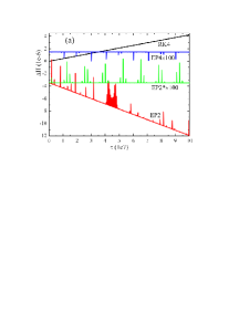
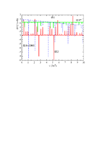
Figure 1: Hamiltonian errors $\Delta H=-1-2H$ in Equation (20) when several known numerical integration algorithms acting on the original Hamiltonian system (18) for massive particles. The algorithms include the second-order implicit and explicit mixed symplectic method IE2, the second-order explicit extended phase-space symplectic-like algorithm EP2, the fourth-order implicit and explicit mixed symplectic method IE4, the fourth-order explicit extended phase-space symplectic-like algorithm EP4 and the fourth-order Runge-Kutta scheme RK4. The parameters are taken as $E=0.995$, $L=4.6$ and $a=0.5$. The initial conditions of an orbit are $r=11$, $\theta=\pi/2$, $p_{r}=0$ and $p_{\theta}>0$ given by Equation (17). All integrations are performed in the proper time. The proper time step is $h=0.1$ for EP2*, $h=4$ for IE4*, and $h=1$ for the other methods. The notation EP2*$\times$100 means that the plotted errors for EP2* are enlarged 100 times, compared with the realistic errors.

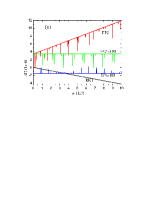
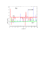
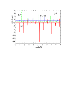
Figure 2: Accuracy of the time-transformed Hamiltonian (26), $\Delta H=2\mathcal{H}$. Panels (a) and (b) correspond to Figures 1 (a) and (b). Panel (c) relates to the new second- and fourth-order explicit symplectic integrators S2 and S4. All computations are implemented in the new coordinate time $w$. The coordinate time step is $h=1$ for S2 and S4, and $h=4$ for S4*.

Table 1: Computational cost [i.e. CPU times (minute^′ second^′′)] for the algorithms in Figs. 1 and 2.

Method	RK4	EP2	EP2*	IE2	EP4	IE4	IE4*	S2	S4	S4*
Fig. 1	$2^{\prime}4^{\prime\prime}$	$1^{\prime}33^{\prime\prime}$	$15^{\prime}45^{\prime\prime}$	$1^{\prime}53^{\prime\prime}$	$3^{\prime}37^{\prime\prime}$	$5^{\prime}48^{\prime\prime}$	$1^{\prime}33^{\prime\prime}$	/	/	/
Fig. 2	$1^{\prime}51^{\prime\prime}$	$1^{\prime}21^{\prime\prime}$	$13^{\prime}43^{\prime\prime}$	$1^{\prime}43^{\prime\prime}$	$3^{\prime}8^{\prime\prime}$	$5^{\prime}26^{\prime\prime}$	$1^{\prime}27^{\prime\prime}$	$57^{\prime\prime}$	$2^{\prime}50^{\prime\prime}$	$43^{\prime\prime}$

5 Numerical evaluations

Compared with the newly proposed integrators, several existing numerical methods are considered. They are RK4, fourth-order implicit and explicit mixed symplectic algorithm (IE4), and fourth-order extended phase-space explicit symplectic-like method (EP4).

5.1 Integrating the original Hamiltonian $H$ with the existing algorithms

The sum of the second and third terms in Equation (18) is labeled as $K$. It is solved in terms of the second-order implicit midpoint rule (Feng 1986). Its corresponding operator is $IM2(h)$, where $h$ is a proper time step. $F$ in Equation (18) is easily solvable and corresponds to an operator $\psi^{F}_{h}$. The two operators symmetrically compose a second-order implicit and explicit mixed symplectic integrator for the original Hamiltonian $H$ in Equation (18)

$$IE2(h)=\psi^{K}_{h/2}\circ IM2(h)\circ\psi^{K}_{h/2}.$$ (45)

The computational efficiency of the method IE2 acting on $H$ is superior to that of the algorithm IM2 acting on $H$. More details on the implicit and explicit mixed symplectic methods were given in the references (Lubich et al. 2010; Zhong et al. 2010; Mei et al. 2013a, 2013b). Similar to the algorithm $S^{\mathcal{H}}_{4}(h)$ in Equation (44), a fourth-order implicit and explicit mixed symplectic algorithm is expressed as

$$IE4=IE2(\gamma h)\circ IE2(\delta h)\circ IE2(\gamma h).$$ (46)

On the other hand, the four-dimensional phase-space variables $(r,\theta,p_{r},p_{\theta})$ of $H$ is extended to eight-dimensional phase-space variables $(r,\theta,\tilde{r},\tilde{\theta},p_{r},$ $p_{\theta},\tilde{p}_{r},\tilde{p}_{\theta})$ in a new Hamiltonian

$$\mathbb{H}=\mathbb{H}_{1}(r,\theta,\tilde{p}_{r},\tilde{p}_{\theta})+\mathbb{H}_{2}(\tilde{r},\tilde{\theta},p_{r},p_{\theta}),$$ (47)

where $\mathbb{H}_{1}(r,\theta,\tilde{p}_{r},\tilde{p}_{\theta})=\mathbb{H}_{2}(\tilde{r},\tilde{\theta},p_{r},p_{\theta})=H(r,\theta,p_{r},p_{\theta})$. $\mathbb{H}_{1}$ and $\mathbb{H}_{2}$ are independently solved in analytical methods. They correspond to operators $\mathcal{A}$ and $\mathcal{B}$ similar to those in Sect. 2. The second- and fourth-order methods $\mathcal{S}^{\mathbb{H}}_{2}$ and $\mathcal{S}^{\mathbb{H}}_{4}$ like those in Equations (5) and (6) can be obtained. For the same initial conditions, the two independent Hamiltonians should have the same solutions: $r=\tilde{r}$, $\theta=\tilde{\theta}$, $\tilde{p}_{r}=p_{r}$ and $\tilde{p}_{\theta}=p_{\theta}$. However, the two solutions are not the same due to their couplings in $\mathcal{S}^{\mathbb{H}}_{2}$ and $\mathcal{S}^{\mathbb{H}}_{4}$. Permutations between the original variables and their corresponding extended variables are necessarily used after the implementation of $\mathcal{S}^{\mathbb{H}}_{2}$ and $\mathcal{S}^{\mathbb{H}}_{4}$ so as to frequently make the two solutions equal (Pihajoki 2015; Liu et al. 2016; Luo et al. 2017; Liu et al. 2017; Luo $\&$ Wu 2017; Li $\&$ Wu 2017; Wu $\&$ Wu 2018). The midpoint permutation method (Luo et al. 2017)

$$\mathcal{M}:\frac{r+\tilde{r}}{2} \rightarrow r=\tilde{r},$$

$$\frac{\theta+\tilde{\theta}}{2} \rightarrow \theta=\tilde{\theta};$$

$$\frac{p_{r}+\tilde{p}_{r}}{2} \rightarrow p_{r}=\tilde{p}_{r},$$ (48)

$$\frac{p_{\theta}+\tilde{p}_{\theta}}{2} \rightarrow p_{\theta}=\tilde{p}_{\theta}$$

is a good choice. The algorithms $\mathcal{S}^{\mathbb{H}}_{2}$ and $\mathcal{S}^{\mathbb{H}}_{4}$ combined with the midpoint permutation are

$$EP2 = \mathcal{M}\otimes\mathcal{S}^{\mathbb{H}}_{2},$$ (49)

$$EP4 = \mathcal{M}\otimes\mathcal{S}^{\mathbb{H}}_{4}.$$ (50)

The symplecticity of $\mathcal{S}^{\mathbb{H}}_{2}$ and $\mathcal{S}^{\mathbb{H}}_{4}$ is destroyed due to the inclusion of $\mathcal{M}$. However, the symmetry makes the methods IE2 and IE4 exhibit good long-term stable behavior in Hamiltonian errors. In this sense, the methods IE2 and IE4 are explicit symplectic-like algorithms for the newly extended phase-space Hamiltonian $\mathbb{H}$ in Equation (47).

Taking the parameters $E=0.995$, $L=4.6$ and $a=0.5$, we choose a test orbit with the initial conditions $r=11$, $\theta=\pi/2$ and $p_{r}=0$. The starting value of $p_{\theta}>0$ is given by Equation (17). The proper time step is $h=1$ and the integration time arrives at $10^{8}$. As shown in Figure 1, RK4 shows a secular drift in Hamiltonian error $\Delta H=-1-2H$ in Equation (20). So does the second-order extended phase-space method EP2. However, this drift is absent in EP2* when the proper time step $h=1$ is replaced with $h=0.1$. It is because the extended phase-space method maintaining the boundness of errors requires appropriate permutations. When the step-size becomes smaller, more permutations are used. This results in the improvement of the algorithm’s accuracy. In fact, the accuracy of EP2* has an order of $\mathcal{O}(10^{-8})$ and is two orders of magnitude higher than that of EP2. The fourth-order extended phase-space method EP4 with the proper time step $h=1$ also gives the same order errors and therefore makes the errors bounded. If the Hamiltonian truncation errors are not larger than the order of $\mathcal{O}(10^{-9})$, $10^{8}$ integration steps yield a great number of roundoff errors that cause the Hamiltonian errors to have a secular growth. The fourth-order implicit and explicit mixed symplectic algorithm IE4 is suitable for this case. When a larger step-size $h=4$ is used, the Hamiltonian errors for IE4* are similar to those for the second-order implicit and explicit mixed symplectic algorithm IE2 with the proper time step $h=1$ and remain stable and bounded.

In short, the algorithms’ performance tested in the above Kerr geometry is very similar to that checked in the Schwarzschild spacetime in Paper I (Wang et al. 2021a).

5.2 Solving time-transformed Hamiltonian $\mathcal{H}$

Without question, the algorithms RK4, IE4 and EP4 are also suited for solving the time-transformed Hamiltonian $\mathcal{H}$ in Equation (26). In addition to them, the new explicit symplectic methods $S^{\mathcal{H}}_{2}$ (labeled as S2) and $S^{\mathcal{H}}_{4}$ (labeled as S4) are respectively used to solve the Hamiltonian splitting form (27). Now, $h$ is a coordinate time step. It is shown by the comparison between Figure 1 and Figures. 2 (a) and (b) that the existing algorithms for the time-transformed Hamiltonian $\mathcal{H}$ and those for the original Hamiltonian $H$ in Equation (18) have no typical differences in the Hamiltonian error behavior. The methods S2 and S4 exhibit good long-term stabilized error behavior in Figure 2 (c). No secular error change exists for S4 because S4 gives the order of $\mathcal{O}(10^{-8})$ to the Hamiltonian errors rather than the order of $\mathcal{O}(10^{-9})$.

The results can be concluded from Figure 2. For the coordinate time step $h=1$, the algorithms RK4, EP2, IE2 and S2 are approximately the same in the Hamiltonian errors; the fourth-order methods EP4, IE4 and S4 are, too. The schemes without secular error drifts are IE2, S2, EP4 and S4. In addition, EP2* with a smaller coordinate time step $h=0.1$ approaches to S4 in accuracy. IE4* and S4* with a larger coordinate time step $h=4$ are close to S2. EP2*, IE* and S4* maintain the boundness of Hamiltonian errors. These similar results are still present when the dynamical parameters and orbits are altered.

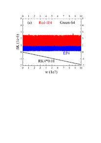
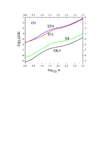
Figure 3: (a) Same as Figure 2, but the fourth-order methods show the errors of the Carter constant for massive particles in Equation (A3). The three methods S4, IE4 and EP4 conserve the Carter constant, but RK4 does not. The notation RK4*0.01 means that the plotted errors for RK4 are decreased 100 times, compared with the realistic errors. IE4 is slightly better than S4 in accuracy of the constant, but is slight poorer than EP4. (b) Accuracy of the solution, estimated by $\Delta\textbf{x}=\mathbf{\bar{x}}-\textbf{x}$, where $\textbf{x}=(r,\theta,p_{r},p_{\theta})$ is given by one of the four algorithms, and $\mathbf{\bar{x}}$ is a high-precision reference solution obtained from an eighth- and ninth-order Runge-Kutta-Fehlberg integrator [RKF8(9)] with adaptive step sizes. For an integration time of $w=2000$, accuracy of the solution is the best for RK4, whereas the poorest for EP4 or IE4.

Besides Hamiltonian $\mathcal{H}$, Carter constant $K$ in Appendix A can be conserved by the algorithms S4, EP4 and IE4, but cannot be conserved by the RK4 method, as shown in Figure 3 (a). RK4 is the poorest in accuracy of the Carter constant, and EP4 is the best. IE4 is slightly better than S4. However, RK4 is the best in accuracy of the solution for an integration time of $w=2000$ in Figure 3 (b), and S4 is better than EP4 or IE4. This shows that RK4 is accurate and efficient for such a short time integration.

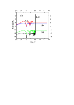
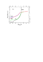
Figure 4: Tests of algorithmic performance for an unstable spherical photon orbit. The new coordinate time step is $h=0.01$. (a) Errors of the Hamiltonian. (b) Errors of the Carter constant. (c) Relative errors of the radius. The errors of the Hamiltonian and Carter constants are the worst when RK4 arrives at an integration time of $w=116$. However, the two constants are conserved by anyone of S4, IE4 and EP4 during an integration time of $w=2000$. Unlike RK4, each of S4, IE4 and EP4 can work well in conservation of the two constants although this orbit does not remain spherical due to orbital instability after the integration time $w=116$.

Testing the performance of these algorithms in Figures 1-3 is based on the boundness of massive particle orbits. What about the performance of these algorithms if the integrated orbits are unstable and unbounded? To answer this question, we adopt the unstable spherical photon orbit B with normalized angular momentum $\Phi=-6$, normalized Carter constant $Q=-13+16\sqrt{2}$ and constant radius $r_{0}=1+2\sqrt{2}$ considered by Bacchini et al. (2018). Some details of the unstable spherical photon orbits are described in Appendix A. When $w=116$ in Figure 4, the orbit begins to run to infinity for RK4, and accuracies of Hamiltonian $\mathcal{H}$ and Carter constant $K$ become the worst. Although this orbit does not remain spherical due to orbital instability, S4, IE4 and EP4 can still work well in conservation of the two constants. In fact, S4 exhibits the best accuracy.

Apart from accuracies of the constants and solutions for these algorithms, computational efficiency should be compared. Table 1 lists CPU times of the algorithms in Figures 1 and 2. S2 has the best efficiency among the three second-order methods S2, IE2 and EP2. The efficiency of S4 is also the best among the efficiencies of the three fourth-order methods S4, IE4 and EP4. This shows the superiority of the application of explicit algorithms in computational efficiency.

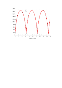
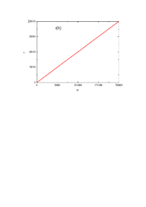
Figure 5: (a) Evolution of $r$ with time for massive particles in Figures 1 and 2. The red line corresponds to the evolution of $r$ with new coordinate time $w$, given by the fourth-order explicit symplectic integrator S4 integrating the time-transformed Hamiltonian (26) with new coordinate time step $h=1$. The black dot relates to the evolution of $r$ with proper time $\tau$, obtained from the fourth-order implicit and explicit mixed symplectic method IE4 solving the original Hamiltonian system (18) with proper time step $h=1$. The former evolution curve is almost consistent with the latter one. (b) The relation between new coordinate time $w$ and proper time $\tau$ for S4 integrating the time-transformed Hamiltonian (26) with new coordinate time step $h=1$. It is clear that the relation is $w=\tau$ if the integration time is not long enough.

Figure 5 (a) plots the evolution curve of $r$ with proper time $\tau$ (colored black dot), obtained by IE4 solving the original Hamiltonian system (18) with the proper time step $h=1$. It also plots the evolution of $r$ with coordinate time $w$ (colored red line), given by S4 integrating the time-transformed Hamiltonian (26) with the coordinate time step $h=1$. The two evolution curves coincide. Here is an explanation. The proper time steps are varied for the use of fixed coordinate time step. However, the coordinate time $w$ and the proper time $\tau$ have no typical differences when S4 solves the Hamiltonian (26) with the coordinate time step, as shown in Figure 5 (b). Clearly, the time transformation function in Equation (25) mainly plays an important role in eliminating the function $\Sigma$ in the denominators of the Hamiltonian (18). Then it leads to successfully implementing the construction of explicit symplectic integrators for the time-transformed Hamiltonian (26). The time transformation function does not have any explicit effect on step-size selection procedures.

5.3 Discussions

The new explicit symplectic integrators are applicable for not only integrating geodesics in the Kerr spacetime, but also the Kerr black hole immersed in an external magnetic field (Kopáček et al. 2010; Kopáček $\&$ Karas 2014; Kopáček $\&$ Karas 2018), Kerr-Newman black hole, and Kerr-Newman black hole with an external magnetic field. The construction of explicit symplectic integrators is based on the splitting of the time-transformed Hamiltonian when the denominators of contravariant metric components $g^{rr}$ and $g^{\theta\theta}$ have $\Sigma$ as a function of $r$ and $\theta$, and the time transformation function $g=\Sigma/r^{2}$ is taken. Such similar constructions are still possibly available if $g^{rr}$ and $g^{\theta\theta}$ have other expressions. In this case, the time transformation function $g$ should need an appropriate choice. In fact, the splitting is valid if the time-transformed Hamiltonian becomes

$$\mathcal{H} = K_{1}(r,\theta)+gg^{rr}p^{2}_{r}+gg^{\theta\theta}p^{2}_{\theta\theta},$$ (51)

$$gg^{rr} = (a_{0}+a_{1}r+\cdots+a_{n}r^{n}+\frac{a_{-1}}{r}+\frac{a_{-2}}{r^{2}}$$ (52)

$$+\cdots+\frac{a_{-m}}{r^{m}})K_{2}(\theta),$$

$$gg^{\theta\theta} = (b_{0}+b_{1}\theta+\cdots+b_{i}\theta^{i}+\frac{b_{-1}}{\theta}+\frac{b_{-2}}{\theta^{2}}$$ (53)

$$+\cdots+\frac{b_{-j}}{r^{j}})K_{3}(r),$$

where $K_{1}$, $K_{2}$ and $K_{3}$ are arbitrary continuous differentiable functions when $r$ and $\theta$ are restricted to $r>2$ and $\theta\neq 0$, and $a_{0}$, $\cdots$, $a_{n}$, $a_{-1}$, $\cdots$, $a_{-m}$, $b_{0}$, $\cdots$, $b_{i}$, $b_{-1}$, $\cdots$, $b_{-j}$ are constant parameters. It is clear that the time-transformed Hamiltonian splitting is desired when time transformation function $g$ satisfies Equations (52) and (53). For example, the time transformation function takes $g=e^{Q-P}$ for $g^{rr}=e^{P-Q}(1-2/r)$ and $g^{\theta\theta}=e^{P-Q}r^{-2}$, where $P$ and $Q$ are functions of $r$ and $\theta$ in an axially symmetric core-shell system (Vieira $\&$ Letelier 1999). Another example is a five-dimensional black ring metric (Igata et al. 2011), where $g^{xx}=(x-y)^{2}(1-x^{2})(1+\nu x)/[R^{2}(1+\lambda x)]$ and $g^{yy}=-(x-y)^{2}(1-y^{2})(1+\nu y)/[R^{2}(1+\lambda x)]$ in ring coordinates $(t,x,y,\phi,\psi)$. Here, $|x|\leq 1$ and $y\leq-1$ are coordinate variables; $R>0$ and $0<\nu\leq\lambda<1$ are constant parameters; $t$, $\phi$ and $\psi$ do not explicitly appear in the metric. Obviously, time transformation function $g=1+\lambda x$ is a good choice. Therefore, the idea for the construction of the present explicit symplectic integrators is not restricted to the Kerr type spacetimes, and is applied to many other relativistic problems.

Although the application of the new algorithms is not wider than that of RAPTOR based on the RK4 scheme (Bronzwaer et al. 2018), accuracies of the new algorithms have an advantage over those of the RK4 scheme in long-term integrations. The new second-order explicit symplectic integrator S2 and RK4 have the same order of magnitude in the Hamiltonian errors in Figures 2 (a) and (c), but they have typical differences in simulations of unstable spherical photon orbits or long-term evolution of massive particle bounded orbits. The errors grow with an increase of integration time for RK4, but remain bounded for S2. When the integration time reaches 116, RK4 gives extremely larger errors to the constants for the unstable spherical photon orbit, but S4 shows smaller errors. When the integration time lasts $10^{10}$, RK4 does not work well and provides uncorrect results to massive particle bounded orbits, whereas S2 still shows no secular growth in the errors. This is an advantage of a symplectic scheme in long-term integrations. In particular, Deng et al. (2020) reported that RK4 combined with manifold correction exhibits poorer performance than the second-order symplectic leapfrog in a $10^{8}$ year integration of the outer solar system involving the Sun and four outer planets. In addition, Figures 2 (a) and (c) clearly show that the new fourth-order explicit symplectic integrator S4 is two orders of magnitude higher than RK4 in accuracy. S4 is typically better than RK4 in numerical performance for the integration of unstable spherical photon orbits.

As shown in Table, the newly proposed algorithms are greatly superior to the implicit and explicit mixed symplectic methods without doubt in terms of computational efficiency. They have also an advantage over the extended phase-space explicit symplectic-like methods EP2 and EP4 because they integrate over 4 dimensions, while the extended phase-space schemes require doubling the phase space (i.e., 8 dimensions). Figures 2 (a) and (c) describe that the extended phase-space method EP2 possesses larger errors than the proposed algorithm S2. Figure 3 (b) shows that EP4 is poorer than S4 in accuracy of the solutions. The methods EP2 and EP4 are in fact similar to the method of Tao (2016) or FANTASY (Christian $\&$ Chan 2021). Wu $\&$ Wu (2018) found that the fourth-order methods like EP4 with the midpoint permutations show better accuracies than the Tao’s method or FANTASY with a good choice of the control constant.

The newly proposed algorithms are inferior to the energy-conserving discrete gradient scheme of Bacchini et al. (2018) in energy conservation, but have some explicit advantages over the latter method. The latter algorithm are implicit, nonsymplectic, and do not preserve other integrals in general (perhaps some integrals may be conserved, as claimed in Footnote 1), but the proposed algorithms are explicit, symplectic, and preserve other integrals like the Carter constant. Therefore, the proposed algorithms are extremely superior to the latter algorithm in computational efficiency. In addition, fourth, sixth orders and higher order schemes are easily available according to the present idea, whereas they are not in terms of the construction method of Bacchini et al.

6 Conclusions

The function $\Sigma$ depending on $r$ and $\theta$ exists in the denominators of the Hamiltonian of Kerr geometry. Thus, explicit symplectic integrators are useless if the Hamiltonian is split into several parts like the Hamiltonian of Schwarzschild spacetimes in the previous papers (Wang et al. 2021a, 2021b, 2021c).

To overcome this difficulty, we use an appropriate time transformation function to eliminate the function $\Sigma$ in the denominators and to obtain a time-transformed Hamiltonian. This Hamiltonian can be separated into five parts with analytical solutions as explicit functions of the new coordinate time, and therefore explicit symplectic integrators are easily available. Numerical tests show that the explicit symplectic methods perform good long-term stable behavior in Hamiltonian errors when appropriate coordinate time steps are chosen. The use of fixed coordinate time steps maintains the symplecticity of the time-transformed Hamiltonian. Although the proper time sizes are variant, there is not an explicit difference between the proper time and newly transformed coordinate time. In this sense, the chosen time transformation function does not mainly play a role in step size selection procedures. The proposed algorithms are superior to the same order extended phase-space explicit symplectic-like methods and implicit and explicit mixed symplectic algorithms in computational efficiency.

The new idea for the construction of such explicit symplectic integrators is not limited to the application of the Kerr metric, and allow for the application of many spacetimes given in Equation (51). This problem will further be considered in our future works.

Appendix A Carter constant and unstable spherical photon orbits

Noticing Equations (18)-(20), we rewrite Equation (18) as follows:

$$-\chi\Sigma=-\frac{E^{2}}{\Delta}(\rho^{4}-\Delta a^{2}\sin^{2}\theta)+\frac{L^{2}(\Delta-a^{2}\sin^{2}\theta)}{\Delta\sin^{2}\theta}+\frac{4ar}{\Delta}EL+\Delta p^{2}_{r}+p^{2}_{\theta},$$ (A1)

where $\chi=1$ for massive particles and $\chi=0$ for massless photons. The equation has the separation of variables:

$$p^{2}_{\theta}+\frac{L^{2}}{\sin^{2}\theta}+E^{2}a^{2}\sin^{2}\theta+\chi a^{2}\cos^{2}\theta=-\chi r^{2}+\frac{E^{2}}{\Delta}\rho^{4}+\frac{L^{2}a^{2}}{\Delta}-\frac{4ar}{\Delta}EL-\Delta p^{2}_{r}.$$ (A2)

Clearly, the left-hand side is a function of variables $\theta$ and $p_{\theta}$, whereas the right-hand side is a function of variables $r$ and $p_{r}$. This equality is possible only when the two sides are equal to same constant

$$K = p^{2}_{\theta}+[\frac{L^{2}}{\sin^{2}\theta}+a^{2}(\chi-E^{2})]\cos^{2}\theta,$$ (A3)

$$K = -L^{2}-a^{2}E^{2}-\chi r^{2}+\frac{E^{2}}{\Delta}\rho^{4}+\frac{L^{2}a^{2}}{\Delta}-\frac{4ar}{\Delta}EL-\Delta p^{2}_{r}.$$ (A4)

Equation (A3) or (A4) is an expressional form of the Carter constant.

Equation (A4) is rewritten as

$$\Sigma^{2}(\frac{dr}{d\tau})^{2}=-(K+L^{2}+a^{2}E^{2}+\chi r^{2})\Delta+E^{2}\rho^{4}+L^{2}a^{2}-4arEL=R(r).$$ (A5)

When $R(r)=dR(r)/dr=0$ in Equation (A5), $r$ corresponds to a constant radius of spherical photon orbit. Teo (2003) studied such spherical photon orbits with normalized angular momentum $\Phi$ and normalized Carter constant $Q$:

$$\Phi = \frac{L}{E}=-\frac{r^{3}-3r^{2}+a^{2}(r+1)}{a(r-1)},$$ (A6)

$$Q = \frac{K}{E^{2}}=-\frac{r^{3}(r^{3}-6r^{2}+9r-4a^{2})}{[a(r-1)]^{2}}.$$ (A7)

These two expressions were also provided by Chan et al. (2018). Due to $d^{2}R(r)/dr^{2}>0$, these orbits would be unstable when they are suffered from perturbations in the radial direction. Müller $\&$ Grave (2010) gave the expression of $E$ as follows:

$$E=\left(\sqrt{\frac{A}{\Sigma\Delta}}-\frac{2ra\Phi}{\sqrt{A\Sigma\Delta}}\right)^{-1}.$$ (A8)

Thus, the other two parameters are easily determined by

$$L=E\Phi,~{}~{}~{}~{}~{}~{}~{}~{}K=QE^{2}.$$ (A9)

For given parameters $r$ and $a=1$ with the initial value $\theta=\pi/2$, we use Equation (A3) to obtain the initial value

$$p_{\theta}=E\sqrt{Q}.$$ (A10)

Appendix B Implementation of algorithm $S^{\mathcal{H}}_{2}$

Codes of the method in Equation (43) are written in the following forms

$$\theta^{\ast} = \theta_{0}+\frac{h}{2}\frac{p_{\theta 0}}{r^{2}_{0}},$$

$$p^{\ast}_{r} = p_{r0}+\frac{h}{2}\frac{p^{2}_{\theta 0}}{r^{3}_{0}};$$

$$r^{\star} = (\frac{h}{r_{0}}a^{2}p^{\ast}_{r}+r^{2}_{0})^{1/2},$$

$$p^{\star}_{r} = \frac{p^{\ast}_{r}}{r_{0}}(\frac{h}{r_{0}}a^{2}p^{\ast}_{r}+r^{2}_{0})^{1/2};$$

$$r^{{\dagger}} = [(r^{\star 2}-\frac{3}{2}hp^{\star}_{r})^{2}/r^{\star}]^{1/3},$$

$$p^{{\dagger}}_{r} = p^{\star}_{r}[(r^{\star 2}-\frac{3}{2}hp^{\star}_{r})/r^{\star 2}]^{1/3};$$

$$r^{{\ddagger}} = r^{{\dagger}}+\frac{h}{2}p^{{\dagger}}_{r};$$

$$p^{\sharp}_{r} = p^{{\dagger}}_{r}+hP_{r}(r^{{\ddagger}},\theta^{\ast}),$$

$$\tau_{1} = \tau_{0}+hg(r^{{\ddagger}},\theta^{\ast}),$$

$$p_{\theta 1} = p_{\theta 0}+hP_{\theta}(r^{{\ddagger}},\theta^{\ast});$$

$$r^{\natural} = r^{{\ddagger}}+\frac{h}{2}p^{\sharp}_{r};$$

$$r^{\diamondsuit} = [(r^{\natural 2}-\frac{3}{2}hp^{\sharp}_{r})^{2}/r^{\natural}]^{1/3},$$

$$p^{\diamondsuit}_{r} = p^{\sharp}_{r}[(r^{\natural 2}-\frac{3}{2}hp^{\sharp}_{r})^{2}/r^{\natural 2}]^{1/3};$$

$$p^{\heartsuit}_{r} = \frac{p^{\diamondsuit}_{r}}{r^{\diamondsuit}}(\frac{h}{r^{\diamondsuit}}a^{2}p^{\diamondsuit}_{r}+r^{\diamondsuit 2})^{1/2},$$

$$r_{1} = (\frac{h}{r^{\diamondsuit}}a^{2}p^{\diamondsuit}_{r}+r^{\diamondsuit 2})^{1/2};$$

$$p_{r1} = p^{\heartsuit}_{r}+\frac{h}{2}\frac{p^{2}_{\theta 1}}{r^{3}_{1}},$$

$$\theta_{1} = \theta^{\ast}+\frac{h}{2}\frac{p_{\theta 1}}{r^{2}_{1}}.$$

In this way, the solutions $(\tau_{1},r_{1},\theta_{1},p_{r1},p_{\theta 1})$ are outputted after the values $(\tau_{0},r_{0},\theta_{0},p_{r0},p_{\theta 0})$ advance a fixed coordinate time step $h$.

Appendix C Other choices of time transformation function

In principle, the time transformation function has various choices. For instance, it is given by

$$g_{1}=\frac{\Sigma}{r}=r+\frac{1}{r}a^{2}\cos^{2}\theta.$$ (C1)

The new coordinate time in Equation (23) becomes $w_{1}$. Advancing the fixed coordinate time $\Delta w_{1}=h$ means advancing a variable proper time $\Delta\tau_{1}\approx rh$. The advancement of proper time is absolutely dominated by the radial separation $r$. When a particle approaches to the central black hole, $\Delta\tau_{1}$ is smaller; but it becomes larger when the particle moves always from the central object. This kind of step-size selection procedure uses adaptive time steps, and satisfies the realistic need on the improvement of numerical precisions. An important contribution for the use of time transformation equation is that this transformation brings the implementation of symplectic integrators with adaptive time step controls. This is the main result claimed in the paper of Mikkola (1997). In terms of the time transformation function $g_{1}$, another new time-transformed Hamiltonian has four separable parts

$$\mathcal{H}^{\ast}=\mathcal{H}^{\ast}_{1}+\mathcal{H}^{\ast}_{2}+\mathcal{H}^{\ast}_{3}+\mathcal{H}^{\ast}_{4},$$ (C2)

where these parts are

$$\mathcal{H}^{\ast}_{1} = \frac{\Sigma}{r}(F+p_{0}),$$ (C3)

$$\mathcal{H}^{\ast}_{2} = (\frac{r}{2}-1)p^{2}_{r},$$ (C4)

$$\mathcal{H}^{\ast}_{3} = \frac{a^{2}}{2r}p^{2}_{r},$$ (C5)

$$\mathcal{H}^{\ast}_{4} = \frac{1}{2r}p^{2}_{\theta}.$$ (C6)

Like the method $S^{\mathcal{H}}_{2}$, another new explicit second-order symplectic integrator for $\mathcal{H}^{\ast}$ reads

$$S^{\mathcal{H}^{\ast}}_{2}(h)=\tilde{\mathcal{H}}^{\ast}_{4}(\frac{h}{2})\circ\tilde{\mathcal{H}}^{\ast}_{3}(\frac{h}{2})\circ\tilde{\mathcal{H}}^{\ast}_{2}(\frac{h}{2})\circ\tilde{\mathcal{H}}^{\ast}_{1}(h)\circ\tilde{\mathcal{H}}^{\ast}_{2}(\frac{h}{2})\circ\tilde{\mathcal{H}}^{\ast}_{3}(\frac{h}{2})\circ\tilde{\mathcal{H}}^{\ast}_{4}(\frac{h}{2}).$$ (C7)

A fourth-order method $S^{\mathcal{H}^{\ast}}_{4}$ can also be obtained. The new explicit symplectic algorithms in the new coordinate time $w_{1}$ are similar to those in the proper time of Schwarzschild spacetime geometry in Paper I (Wang et al. 2021a).

If the time transformation function takes the form

$$g_{2}(r,\theta)=\Sigma,$$ (C8)

the new coordinate time in Equation (23) is $w_{2}$. In this case, Equation (24) corresponds to a simpler time-transformed Hamiltonian

$$\mathcal{H}^{\star}=\Sigma(F+p_{0})+\frac{\Delta}{2}p^{2}_{r}+\frac{1}{2}p^{2}_{\theta}.$$ (C9)

It has three separable parts

$$\mathcal{H}^{\star}=\mathcal{H}^{\star}_{1}+\mathcal{H}^{\star}_{2}+\mathcal{H}^{\star}_{3},$$ (C10)

where the sub-Hamiltonians are

$$\mathcal{H}^{\star}_{1} = \Sigma(F+p_{0}),$$ (C11)

$$\mathcal{H}^{\star}_{2} = \frac{1}{2}r^{2}p^{2}_{r},$$ (C12)

$$\mathcal{H}^{\star}_{3} = \frac{1}{2}(a^{2}-2r)p^{2}_{r}+\frac{1}{2}p^{2}_{\theta}.$$ (C13)

Obviously, the three parts are independently solved in analytical methods and their analytical solutions are explicit functions of the new coordinate time $w_{2}$. Using Lie operators $\tilde{\mathcal{H}}^{\star}_{1}$, $\tilde{\mathcal{H}}^{\star}_{2}$ and $\tilde{\mathcal{H}}^{\star}_{3}$ to represent the analytical solutions of $\mathcal{H}^{\star}_{1}$, $\mathcal{H}^{\star}_{2}$ and $\mathcal{H}^{\star}_{3}$, we easily obtain an explicit second-order symplectic integrator for the system $\mathcal{H}^{\star}$ as follows

$$S^{\mathcal{H}^{\star}}_{2}(h)=\tilde{\mathcal{H}}^{\star}_{3}(\frac{h}{2})\circ\tilde{\mathcal{H}}^{\star}_{2}(\frac{h}{2})\circ\tilde{\mathcal{H}}^{\star}_{1}(h)\circ\tilde{\mathcal{H}}^{\star}_{2}(\frac{h}{2})\circ\tilde{\mathcal{H}}^{\star}_{3}(\frac{h}{2}).$$ (C14)

An explicit fourth-order symplectic integrator $S^{\mathcal{H}^{\star}}_{4}$ can be easily available, too. As a point to illustrate, the newly fixed coordinate time step $\Delta w_{2}=h$ corresponds to a variant proper time step $\Delta\tau_{2}\approx r^{2}h$.

For $r\gg 1$, the fixed coordinate time steps $\Delta w_{1}\ll 1$ and $\Delta w_{2}\ll 1$ should be required when the variant proper time steps $\Delta\tau_{1}$ and $\Delta\tau_{2}$ are 1. Such extremely small coordinate time steps would lead to fatal roundoff errors. Thus, we take the time transformation function (25) rather than Equations (C1) and (C8).

References

- Abbott et al. (2016) Abbott, B. P., Abbott, R., Abbott, T. D., et al. 2016, PhRvL, 116, 241102
- Abbott et al. (2020) Abbott, R., Abbott, T. D., Abraham, S., et al. 2020, ApJL, 900, L13
- Bacchini et al. (2018a) Bacchini, F., Ripperda, B., Chen, A. Y., Sironi, L. 2018, ApJS, 237, 6
- Bacchini et al. (2018b) Bacchini, F., Ripperda, B., Chen, A. Y., Sironi, L. 2019, ApJS, 240, 40
- Bronzwaer et al. (2018) Bronzwaer, T., Davelaar, J., Younsi, Z., Mościbrodzka, M., Falcke, H., Kramer, M., Rezzolla, L. 2018, AA, 613, A2
- Bronzwaer et al. (2020) Bronzwaer, T., Younsi, Z., Davelaar, J., Falcke, H. 2020, AA, 641, A126
- Brown (2006) Brown, J. D. 2006, Phys. Rev. D, 73, 024001
- Carter (1968) Carter, B. 1968, Phy. Rev., 174, 1559
- Chambers & Murison (2000) Chambers, J. E., Murison, M. A. 2000, AJ, 119, 425
- Chan et al. (2018) Chan, C., Medeiros, L., Özel, F., Psaltis, D. 2018, ApJ, 867, 59
- Christian & Chan (2018) Christian, P., Chan, C. 2021, ApJ, 909, 67
- Deng et al. (2020) Deng, C., Wu, X., Liang, E. 2020, MNRAS, 496, 2946
- Collaboration et al. (2019) EHT Collaboration, et al. 2019, ApJL, 875, L1 (Paper I)
- Emel’yanenko (2007) Emel’yanenko, V. V. 2007, Celest. Mech. Dyn. Astron., 98, 191
- Feng (1986) Feng, K. 1986, Journal of Computational Mathematics, 44, 279
- Forest & Ruth (1990) Forest, E., Ruth, R. D. 1990, Physica D, 43, 105
- Fukushima (2003) Fukushima, T. 2003, AJ, 126, 1097
- Hairer et al. (1999) Hairer, E., Lubich, C. Wanner, G. 1999, Geometric Numerical Integration, Springer-Verlag, Berlin
- Hu et al. (2019) Hu, S., Wu, X., Huang, G., Liang, E. 2019, ApJ, 887, 191
- Hu et al. (2021) Hu, S., Wu, X., Liang, E. 2021, ApJS, 253, 55
- Igata et al. (2011) Igata, T., Ishihara, H., Takamori, Y. 2011, Phys. Rev. D, 83, 047501
- Kerr (1963) Kerr, R. P. 1963, Phy. Rev. Lett., 11, 237
- Kopáček & Karas (2014) Kopáček, O., Karas, V. 2014, ApJ, 787, 117
- Kopáček & Karas (2018) Kopáček, O., Karas, V. 2018, ApJ, 853, 53
- Kopáček et al. (2010) Kopáček, O., Karas, V., Kovář, J., Stuchlík, Z. 2010, ApJ, 722, 1240
- Laskar & Robutel (2001) Laskar J., Robutel, P. 2001, Celest. Mech. Dyn. Astron., 80, 39
- Li & Wu (2017) Li D., Wu, X. 2017, Mon. Not. R. Astron. Soc., 469, 3031
- Li & Wu (2019) Li, D., Wu, X. 2019, Eur. Phys. J. Plus, 134, 96
- Liu et al. (2016) Liu, L., Wu, X., Huang, G. Q., Liu, F. 2016, Mon. Not. R. Astron. Soc., 459, 1968
- Lubich et al. (2010) Lubich, C., Walther, B., Brügmann, B. 2010, Phys. Rev. D, 81, 104025
- Luo et al. (2017) Luo, J., Wu, X., Huang, G., Liu, F. 2017, ApJ, 834, 64
- Ma et al. (2008a) Ma, D. Z., Wu, X., Zhong, S. Y. 2008a, ApJ, 687, 1294
- Mei et al. (2013a) Mei, L., Ju, M., Wu, X., Liu, S. 2013a, Mon. Not. R. Astron. Soc., 435, 2246
- Mei et al. (2013b) Mei, L., Wu, X., Liu, F. 2013b, Eur. Phys. J. C, 73, 2413
- Mikkola (1997) Mikkola, S. 1997, Celest. Mech. Dyn. Ast., 67, 145
- Mikkola & Aarseth (2002) Mikkola, S., Aarseth, S. 2002, Celest. Mech. Dyn. Ast., 84, 343
- Mikkola & Tanikawa (1999) Mikkola, S., Tanikawa, K. 1999, Celest. Mech. Dyn. Ast., 74, 287
- Mikkola & Tanikawa (2013) Mikkola, S., Tanikawa, K. 2013, New Astronomy, 20, 38
- Müller & Grave (2010) Müller, T., Grave, F. 2010, CPC, 181, 413
- Nacozy (1971) Nacozy, P. E. 1971, Astrophys. Space Sci, 14, 40
- Ni & Wu (2014) Ni, X. T., Wu, X. 2014, Res. Astron. Astrophys., 14, 1329
- Omelyan et al. (2003) Omelyan, I. P., Mryglod, I. M., Folk, R. 2003, Comput. Phys. Commun., 151, 272
- Pihajoki (2015) Pihajoki, P. 2015, Celest. Mech. Dyn. Astron., 121, 211
- Preto & Saha (2009) Preto, M., Saha, P. 2009, ApJ, 703, 1743
- Preto & Tremaine (1999) Preto, M., Tremaine, S. 1999, AJ, 118, 2532
- Ruth (1983) Ruth, R. D, 1983, IEEE Trans. Nucl. Sci. NS 30, 2669
- Swope et al. (1982) Swope, W. C., Andersen, H. C., Berens, P. H., Wilson, K. R. 1982, J. Chem. Phys. 76, 637
- Takahashi & Koyama (2009) Takahashi, M., Koyama, H. 2009, ApJ, 693, 472
- Tao (2016) Tao, M. 2016, Phys. Rev. E, 94, 043303
- Teo (2003) Teo, E. 2003, GReGr, 35, 11
- Tsang et al. (2015) Tsang, D., Galley, C. R., Stein, L. C., Turner, A. 2015, ApJL, 809, L9
- Vieira & Letelier (1999) Vieira, W. M., Letelier, P. S. 1999, ApJ, 513, 383
- Wang & Nitadori (2020) Wang, L., Nitadori, K. 2020, Mon. Not. R. Astron. Soc., 497, 4384
- Wang et al. (2021a) Wang Y., Sun W., Liu F., Wu X. 2021a, ApJ, 907, 66 (Paper I)
- Wang et al. (2021b) Wang Y., Sun W., Liu F., Wu X., 2021b, ApJ, 909, 22 (Paper II)
- Wang et al. (2021c) Wang Y., Sun W., Liu F., Wu X., 2021c, ApJS, accepted (Paper III)
- Wang et al. (2016) Wang, S. C., Wu, X., Liu, F. Y. 2016, MNRAS, 463, 1352
- Wang et al. (2018) Wang, S. C., Huang, G. Q., Wu, X. 2018, AJ, 155, 67
- Wisdom (1982) Wisdom, J. 1982, AJ, 87, 577
- Wisdom & Holman (1991) Wisdom, J., Holman, M. 1991, AJ, 102, 1528
- Wu et al. (2003) Wu, X., Huang, T. Y., Wan, X. S., Zhang, H. 2007, AJ, 133, 2643
- Wu & Wu (2018) Wu, Y. L., Wu, X. 2018, International Journal of Modern Physics C, 29, 1850006
- Yoshida (1990) Yoshida, H. 1990, Phys. Lett. A, 150, 262
- Zhong et al. (2010) Zhong, S. Y., Wu, X., Liu, S. Q., Deng, X. F. 2010, Phys. Rev. D, 82, 124040