High-Dimensional Methods for Quantum Homodyne Tomography

Abstract

We provide optimized recursion relations for homodyne tomography. We improve previous methods by mitigating the divergences intrinsic in the calculation of the pattern functions used previously, and detail how to implement the data analysis through Monte Carlo simulations. Our refinements are necessary for the reconstruction of excited quantum states which populate a high-dimensional subspace of the electromagnetic field Hilbert space. We also present a Julia package for the analysis and the reconstruction method.

Quantum tomography is the procedure that reconstructs the quantum state of a system from repeated measurements of a (complete) set of observables on a number of copies of equally prepared quantum systems. This is the only way to measure a quantum state: indeed, on one hand it is impossible to recover the state from a single copy of the system D’Ariano and Yuen (1996); on the other, without the measurement of a complete set of observables (a quorum), there is not enough information for the reconstruction as different states may give the exact same statistics on an incomplete set of observables. The same quantum systems may have different possible quorums D'Ariano et al. (2000). For the state of a single mode of the radiation field there are two quorums that are typically used: either the field quadratures $X_{\varphi}=\frac{1}{2}(a^{\dagger}e^{i\varphi}+ae^{-i\varphi})$ D’Ariano et al. (2003, 2004, 2007) or the displaced parity operator $D^{\dagger}(\alpha)(-1)^{a^{\dagger}a}D(\alpha)$ Lutterbach and Davidovich (1997), where $a$ is the annihilation operator of the mode and $D(\alpha)=e^{\alpha a^{\dagger}-\bar{\alpha}a}$ is the displacement operator. In this paper we will focus on the former, which can be detected straightforwardly with a homodyne detector D’Ariano et al. (2007). The homodyne measurements are the marginal probability distributions of each quadrature $X_{\varphi}$, collectively giving the Radon transform of the Wigner function. As such, the seminal early homodyne tomography method employed Radon transform inversion techniques Vogel and Risken (1989). This method, thus, requires the homodyne data to be binned in order to obtain a distribution. This introduces a bias in the reconstruction, due to the width of the binning. The Homodyne Computed Tomography (HCT) method, proposed in D’Ariano et al. (1994) and refined in Paul et al. (1995); D’Ariano et al. (1995); Leonhardt et al. (1995), avoids this problem by directly reconstructing the quantum state—or expectation values of arbitrary operators—without going through the Wigner function. Hence, one could in principle use a single data point for each homodyne measurement (no binning) to ensure complete unbiasedness. Alternative procedures use maximum likelihood methods Rossi (2018), which produce very high-quality reconstructions, but they are biased and, especially, completely unsuited for the high-dimensional states that we consider here: the minimization procedures entailed become rapidly intractable for large dimensions.

In this paper we provide a (small) further refinement of the HCT method to tame numerical instabilities, and present a Julia package from which some extremely high-dimensional Monte Carlo simulations of reconstructions are obtained to illustrate the method. These show that quantum states with density matrices of one order of magnitude larger than the size of previous simulations and experiments can be reconstructed. This is timely since quantum tomography is starting to be used in microwave cavities Vlastakis et al. (2013); Eichler et al. (2011, 2012); Mallet et al. (2011), where even small signals entail huge number of photons, i.e. a high-dimensional subspace of the radiation Hilbert space because of the low energy of each microwave photon.

The outline follows: in Section I we provide a bare-bones description of the method; in Section II we describe how one can produce a numerical algorithm that implements it, and we illustrate it with simulated experiments; in Section III we describe the software packages used for this work; and, finally, in Section IV we draw our conclusions regarding the work presented in this paper. In Appendix A we review the derivation of the method and in Appendix B we derive the optimized recursion relations for the calculation of the Wigner function.

I Homodyne Tomography

The homodyne detector is an apparatus that measures the quadrature observable $X_{\varphi}$ at optical frequencies. Similar devices can be built for microwave cavities, e.g. Eichler et al. (2011); Mallet et al. (2011). This apparatus receives as input a number $\varphi\in[0,\pi]$, which typically refers to the phase of a local oscillator in an intense coherent state. It outputs a real number $x$, which (once calibrated) denotes the measured value of the quadrature $X_{\varphi}$ identified by $\varphi$. The data taking stage of the homodyne tomography experiment then resorts in choosing $n_{\varphi}$ values $\varphi_{i}$ of the phase and measuring $n_{q}$ quadrature values $x_{i}$ for each chosen phase. Ideally, one should choose $n_{q}=1$ (i.e. use a different phase for each quadrature measurement) to avoid a possible source of bias, but it is known Leonhardt and Munroe (1996), and confirmed by our simulations (e.g. Fig. 1), that this is not a big concern if the number of phases $n_{\varphi}$ is sufficiently large (more excited states requiring a larger number of phases). Using fixed phases simplifies the experiment considerably. The $n_{\varphi}$ phases must be chosen uniformly in the interval $[0,\pi]$ or, more conveniently for the numerical implementation, in the interval $[0,2\pi]$: due to the phase space symmetries, the two intervals are equivalent as discussed below.

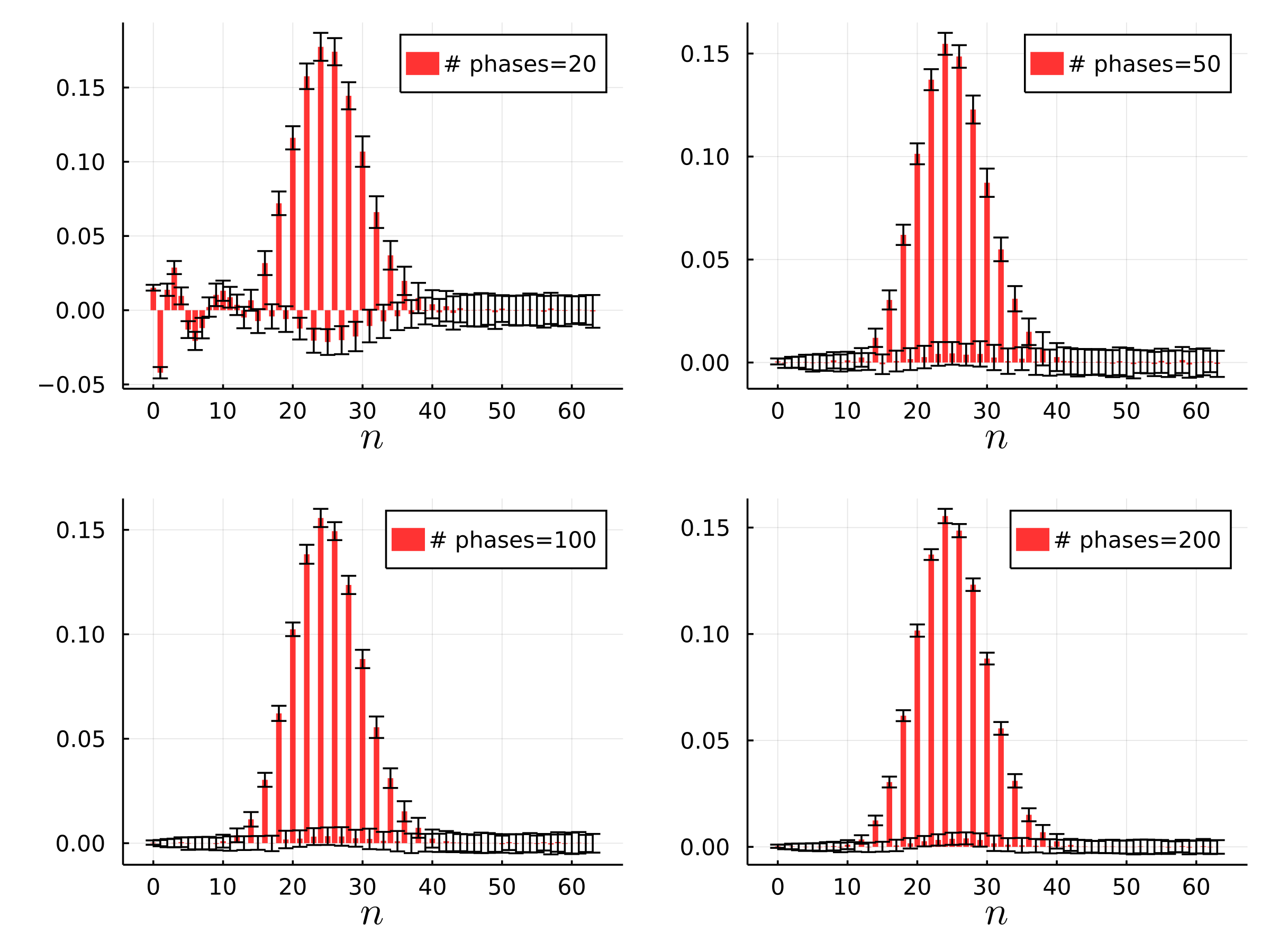
Figure 1: Effect of the number of phases: the pictured tomographic reconstructions (diagonal of the density matrix) use the same number of quadrature results $n_{\textup{bin}}=400$ for different values of the number of quadrature phases $n_{\varphi}\in\{20,50,100,200\}$. The reconstructions rapidly converge to a good quality already for relatively small numbers of phases. The reconstructions refer to a Schrödinger cat state $\propto\ket{\alpha}+\ket{-\alpha}$ with $\alpha=5$ and density matrix cut-off $M=64$. The data was generated with a Monte Carlo simulation with $1000$ quadrature measurements and $100$ statistical blocks for a total of $1000\times 100$ measurements for each phase.

The result of the experiment is a set of data $\{(\varphi_{k},x_{k})\}_{k\in I_{N}}$, $I_{N}=\set{0,\dots,N-1}$, where $x_{k}$ is the result of the $k$-th measurement in which the quadrature $X_{\varphi_{k}}$ was measured and $N=n_{\varphi}n_{q}$ is the total number of measurements.

Now we detail how this data can be used for the tomographic reconstruction. Importantly, the HCT method allows for the direct reconstruction of the expectation value $\braket{O}$ of any operator, not necessarily an observable. As an illustrative example, we now show how one can reconstruct the density matrix $\rho_{nm}=\braket{n}{\rho}{m}$ written on the Fock basis. This is achieved by using the non-Hermitian $O=\ket{m}\!\!\mkern 2.0mu\bra{n}$, since $\braket{O}=\mathrm{Tr}[\rho\ket{m}\!\!\mkern 2.0mu\bra{n}]=\braket{n}{\rho}{m}$. It can be shown (see Appendix, Eq. 19) that the matrix element can be written as

$$\rho_{n,m}=\frac{1}{\pi}\int_{0}^{\pi}\!\!\!\mathrm{d}\mkern 0.0mu\varphi\,e^{-i(m-n)\varphi}\int_{R}\mathrm{d}\mkern 0.0mux\,p_{\varphi}(x)f_{n,m}(x),$$ (1)

where $f_{n,m}$ are pattern functions defined below and $p_{\varphi}(x)={}_{\varphi}\!\braket{x}{\rho}{x}_{\varphi}$ is the conditional probability of obtaining outcome $x$ given that the $\varphi$-quadrature was measured, namely the outcome relative to the eigenstate $\ket{x}_{\varphi}$ of $X_{\varphi}$. Since, by construction, the phases $\varphi_{i}$ are uniform in the interval $[0,\pi]$, we can interpret $1/\pi$ as the uniform probability of choosing the phase $\varphi$; then, from Bayes rule, the joint probability of choosing a phase $\varphi$ and obtaining a $\varphi$-quadrature outcome $x$ is $p_{\varphi}(x)/\pi$. Thus we can use the collected data $\{(\varphi_{k},x_{k})\}_{k\in I_{N}}$ to calculate the double integral of Eq. 1 as a Monte Carlo integral:

$$\rho_{n,m}=\frac{1}{N}\sum_{k=0}^{N-1}e^{-i(m-n)\varphi_{k}}f_{n,m}(x_{k})\pm\Delta_{N},$$ (2)

where $\Delta_{N}$ is the error due to the finite $N$. Indeed, the equality is strict only in the limit $N\to\infty$ (when $\Delta_{N}\to 0$), which of course cannot be reached experimentally. However, since we are using Monte Carlo integration, the error $\Delta_{N}$ for finite $N$ is strictly a statistical error only, which can be easily evaluated from the variance $\sigma^{2}$ of the data:

$$\Delta_{N}=\sqrt{\frac{\sigma^{2}}{N}}=\\ \sqrt{\frac{1}{N(N-1)}\left[\textstyle\sum_{k}F^{2}(\varphi_{k},x_{k})-\big{(}\textstyle\sum_{k}F(\varphi_{k},x_{k})\big{)}^{2}\right]},$$ (3)

with $F(\varphi_{k},x_{k})=e^{-i(m-n)\varphi_{k}}f_{n,m}(x_{k})$ (more rigorously, if $m\neq n$, when $F$ is complex, one has to separately evaluate the variance of the real and imaginary parts).

II Numerical implementation

The calculation of the pattern functions Leonhardt et al. (1996, 1995) is quite involved and is reviewed in Appendix A. Starting from the recursion relations derived in the same section, we provide here a simplified form, suitable for numerical evaluation also with non-wide floating point representation, such as the standard 32 bits single precision data type.

To speed up the data analysis, we create a probability distribution by discretizing the possible values of the quadrature $x$ and binning the $n_{q}$ values of the quadrature data $x_{k}$ into $n_{\textup{bin}}$ bins. As discussed above, in contrast to methods based on the inversion of the Radon transform, this is not a fundamental limitation. Indeed, we show in Fig. 2 that our method still works in the regime where $n_{\textup{bin}}\gg n_{q}$, where most bins are unpopulated and at most a handful of data points end up in the same bin. In this regime, the Radon transform inversion would fail, in contrast to HCT. Nonetheless, binning may be useful, since it allows for a faster and more effective reconstruction because one has to calculate the recurrence relation below only once per bin (this is of interest for the reconstruction of huge data sets).

The binning is done by collecting the data into a $n_{\varphi}\times n_{\textup{bin}}$ matrix $S$, called sinogram. Each matrix row $j\in I_{n_{\varphi}}$ represents the quadrature probability at phase $\varphi_{j}$, namely $S_{j,i}$ is the fraction of the $n_{q}$ values of $x_{k}$ that fall into the $i$-th bin, $i\in I_{n_{\textup{bin}}}$. Asymptotically we have that $S_{j,i}\sim p_{\varphi_{j}}(x_{i})$, with $x_{i}$ a representative point in the $i$-th bin. We choose equispaced phases $\varphi_{j}=\frac{2\pi}{n_{\varphi}}j$. Again, this is a matter of numerical convenience: in principle, one should choose the phases with uniform random probability in the interval $[0,2\pi]$. We assume the measurements are taken on the whole interval $[0,2\pi]$ so that we can use the FFT algorithm; if this is not the case—as it is when the samples are taken only in $[0,\pi]$—one can always double the data exploiting the phase space symmetry $X_{\varphi+\pi}=-X_{\varphi}$.

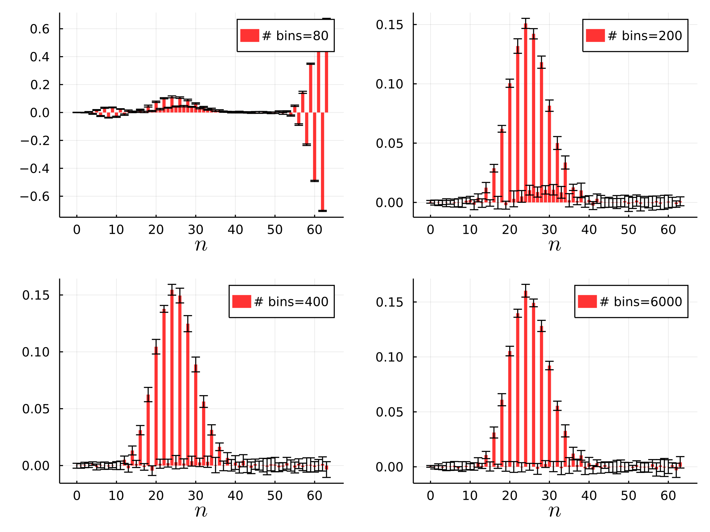
Figure 2: Effect of the data binning. While HCT does not require binning of the homodyne data, it can speed up the data analysis. We show the diagonal of the density matrix with error bars on each element, showing the effect of binning for various bin size: the reconstruction converges quickly when increasing the number of bins $n_{\textup{bin}}$ and gives good results also in the regime $n_{\textup{bin}}\gg 1$, where the inverse Radon transform method fails. The measurements were obtained with a Monte Carlo simulation of $100$ measurements for $10$ statistical blocks with $n_{\varphi}=800$ phases. The simulated state is a Schrödinger cat state $\ket{\psi}\propto\ket{\alpha}+\ket{-\alpha}$, $\alpha=5$ and density matrix dimension $M=64$.

In order to implement the tomographic formula on a computer we have to choose a cutoff for the density matrix. As will be clear in the following, this cutoff does not introduce any bias in the reconstruction, although a sensible (i.e. normalized) reconstruction will be obtained only if such cutoff is chosen sufficiently large. Indeed, one can check a posteriori whether the chosen $M$ is sufficient by looking at the normalization of the reconstructed state, namely by checking if it is compatible with one within the statistical error bars. In the following we will assume the density matrix has dimensions $M\times M$.

By dividing the sum into two parts (along the bins and along the phases), the Monte Carlo integral of Eq. 2 becomes

$$\rho_{n,m}=\sum_{i=0}^{n_{\textup{bin}}-1}\hat{S}_{m-n,i}f_{n,m}(x_{i}),$$ (4)

where the factor $$1/n_{\textup{bin}} \hat{S}$$ is included into the definition of and

$$\hat{S}_{d,i}=\frac{1}{n_{\varphi}}\sum_{j=0}^{n_{\varphi}-1}S_{j,i}e^{-2\pi i\frac{jd}{n_{\varphi}}}$$ (5)

is the one-dimensional discrete Fourier transform (DFT) along the first dimension of $S_{j,i}$.

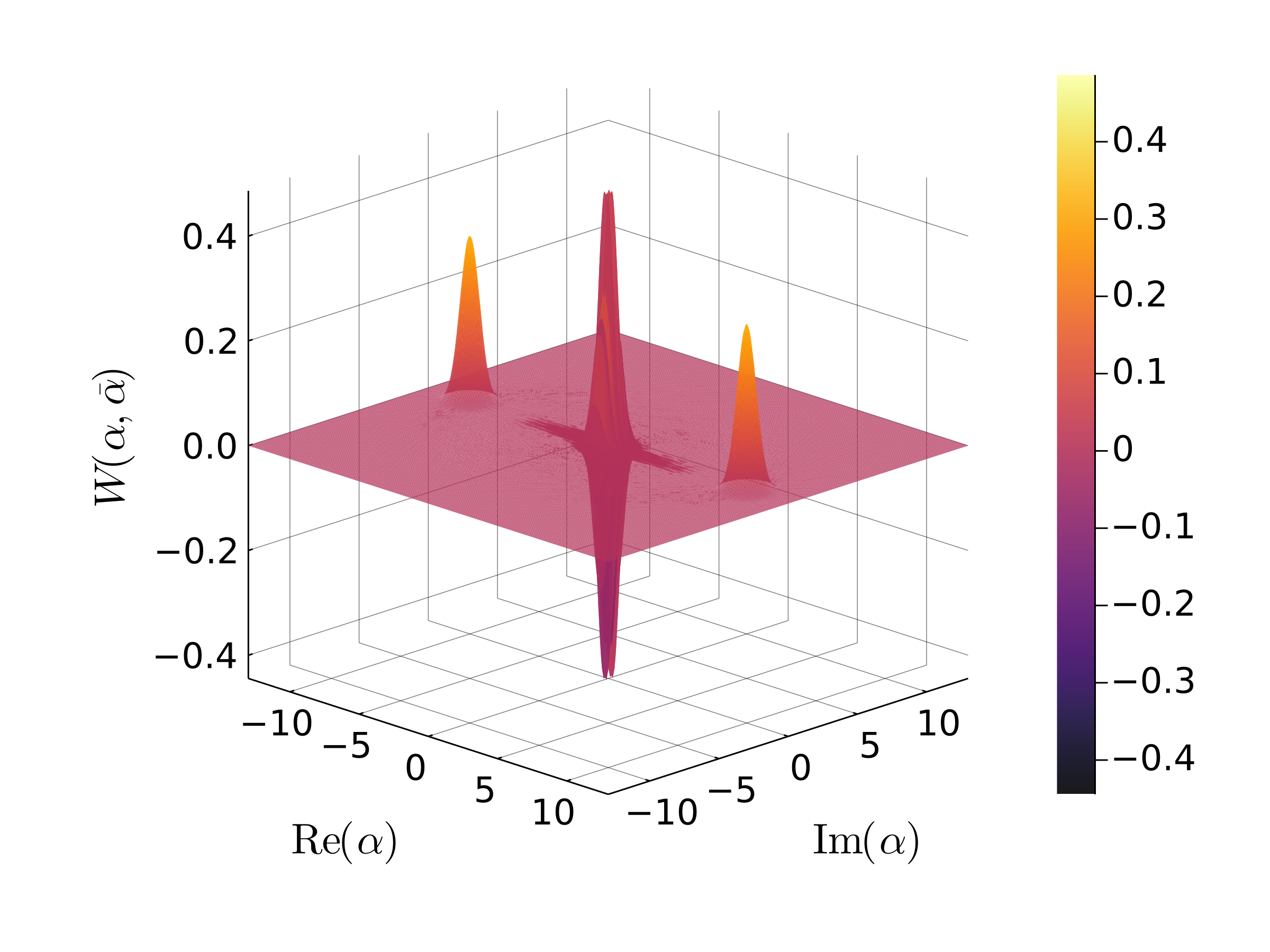
Figure 3: Wigner function $W(\alpha,\bar{\alpha})$ for a Schrödinger cat state $\ket{\psi}\propto\ket{\alpha}+\ket{-\alpha}$, $\alpha=10$, $n_{\textup{bin}}=1000$ and $M=256$; number of samples: $10000$ for $100$ statistical blocks and $n_{\varphi}=800$ phases.

The pattern functions $f_{n,m}$ can be written in the following factorized form D’Ariano et al. (1995); Leonhardt et al. (1995, 1996) (see Appendix A):

$$f_{n,m}(x)=2xu_{n}(x)v_{m}(x)-\phantom{x}\\ \sqrt{n+1}u_{n+1}(x)v_{m}(x)-\phantom{x}\\ \sqrt{m+1}u_{n}(x)v_{m+1}(x),$$ (6)

The vectors $u_{n}$ and $v_{m}$ appear always multiplied together, which means that we can change their definition with respect to their previously published values Leonhardt et al. (1996, 1995) (see Eqs. 29, 31 and 33) for the purposes of the numerical implementation. Furthermore, the square roots $\sqrt{n}$ appear always with the same index of either $u_{n}$ or $v_{m}$, so we introduce additional vectors $\tilde{u}_{n}=\sqrt{n}u_{n}$, $\tilde{v}_{m}=\sqrt{m}v_{m}$ that can be precomputed along with $u_{n}$ and $v_{m}$. Thus, a recursive definition of $u_{n}$ that is better suited for numerics is

$$\begin{cases}&u_{0}=\beta,\quad\tilde{u}_{0}=0,\\ &u_{1}=2xu_{0},\quad\tilde{u}_{1}=u_{1},\\ &\tilde{u}_{n}=2xu_{n-1}-\sqrt{n-2}u_{n-2},\\ &u_{n}=\tilde{u}_{n}/\sqrt{n}.\end{cases}$$ (7)

Here, we introduced a constant $\beta$ to compensate for growth of the sequence $(u_{n})$ and can be arbitrarily chosen to control its range of values. The simulations and reconstruction presented here are obtained with the heuristic choice $\beta\approx\exp(-3\max x)$, where $\max x$ is the maximum obtained homodyne value.

Likewise, the corresponding definition of $v_{m}$ best suited for numerics follows. It is defined through a forward or backward recursion Leonhardt et al. (1996, 1995) depending on the value of $x$. The backward recursion can be used if

$$\lvert x\rvert<\alpha_{4k}-\frac{1}{2}\frac{1}{\sqrt[3]{\alpha_{4k}}},$$ (8)

with $\alpha_{n}=\sqrt{n+1/2}$. Then the recursion can be safely started from $m=4M$:

$$\begin{cases}&v_{4M}(x)=\beta^{-1}e^{-x^{2}}\kappa_{4M},\\ &\tilde{v}_{4M}(x)=\sqrt{4M}v_{4M}(x),\\ &v_{4M-1}(x)=\beta^{-1}e^{-x^{2}}\kappa_{4M-1},\\ &\tilde{v}_{4M-1}(x)=\sqrt{4M-1}v_{4M-1}(x),\\ &v_{m}(x)=\frac{1}{\sqrt{m+1}}(2xv_{m+1}-\sqrt{m+2}v_{m+2}),\\ &\tilde{v}_{m}(x)=\sqrt{m}v_{m}(x).\end{cases}$$ (9)

For values of $x$ outside the region of Eq. 8, one should use the forward recursion

$$\begin{cases}&v_{0}(x)=\frac{\beta^{-1}}{x},\\ &\tilde{v}_{0}(x)=0,\\ &v_{m}(x)=\frac{\sqrt{m}}{2x}v_{m-1}(x),\\ &\tilde{v}_{m}(x)=\sqrt{m}v_{m}(x).\end{cases}$$ (10)

We scaled the starting value by $\beta^{-1}e^{-x^{2}}$ to compensate the divergence of the vectors $v_{m}$ and also canceling the effect of the constant $\beta$, which is needed only to change the range of values assumed by the vectors $u_{n}$ and $v_{m}$. Now the pattern functions $f_{n,m}$ can be rewritten as

$$f_{n,m}(x)=[2xu_{n}(x)-\tilde{u}_{n+1}(x)]v_{m}(x)-\phantom{x}\\ u_{n}(x)\tilde{v}_{m+1}(x).$$ (11)

In Fig. 4 some examples of very large reconstructions of density matrices are presented, which use the above recursions.

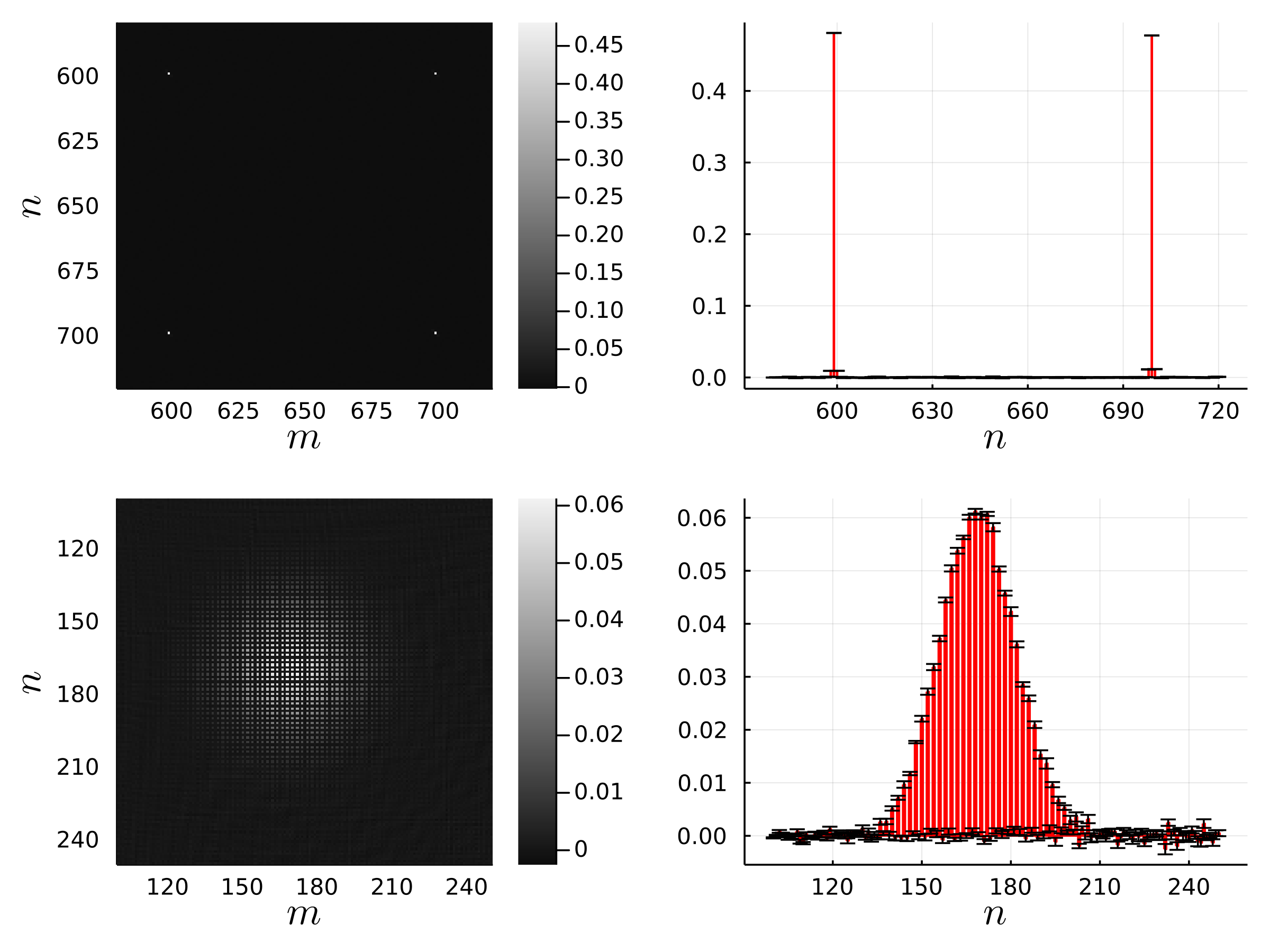
Figure 4: Simulated homodyne reconstructions of large density matrices. Left: the real part of the density matrix is plotted. Right: the diagonal is shown with the error bars on each matrix element. The plots above refer to the state $\ket{\psi}\propto\ket{600}+\ket{700}$, with $1000$ samples for $10$ blocks, $8000$ bins and $M=800$; the plots below to the state $\ket{\psi^{\prime}}\propto\ket{\alpha}+\ket{-\alpha}$, with $\alpha=13$, $M=300$, $6000$ bins, and same statistics. A very small effect of the binning is evident as a slight decrease of the peaks in the upper-right figure.

II.1 Calculating the Wigner function

As discussed above, the HCT method does not require the reconstruction of the Wigner function, as it directly reconstructs the density matrix (and the expectation value of arbitrary operators). Still, it may be useful to calculate also the Wigner function D’ariano (1997), defined as

$$W(\alpha,\bar{\alpha})=\frac{2}{\pi}\mathrm{Tr}\left[\rho e^{2\lparen\alpha a^{\dagger}-\bar{\alpha}a\rparen}e^{i\pi a^{\dagger}a}\right],$$ (12)

which can be explicitly written as

$$W(\alpha,\bar{\alpha})=\frac{2}{\pi}\mathrm{Re}\sum_{d=0}^{+\infty}e^{id\arg{\alpha}}\sum_{n=0}^{+\infty}\Lambda_{n,d}(\lvert 2\alpha\rvert^{2})\rho_{n,n+d},$$ (13)

where $$\rho_{n,m}=\braket{n}{\rho}{m}$$, and

$$\Lambda_{n,d}(x)=(-1)^{n}(2-\delta_{d0})x^{d/2}\sqrt{\frac{n!}{(n+d)!}}\mathcal{L}_{n}^{d}(x).$$ (14)

Here, $\mathcal{L}_{n}^{d}$ is defined as $\mathcal{L}_{n}^{d}(x)=e^{-x/2}L_{n}^{d}(x)$, where $L_{n}^{d}(x)$ are the (generalized) Laguerre polynomials.

The formula in Eq. 14 does not perform well for lower precision data types as there are several quantities that become very large quite fast. Although one can mitigate this by, for instance, computing first the logarithm of the factorials, this may still be not enough for highly excited states that occupy a large part of the phase space. This problem can be solved with appropriately designed recursion relations that we present in Appendix B. The two methods presented there are inequivalent, but have roughly the same efficiency.

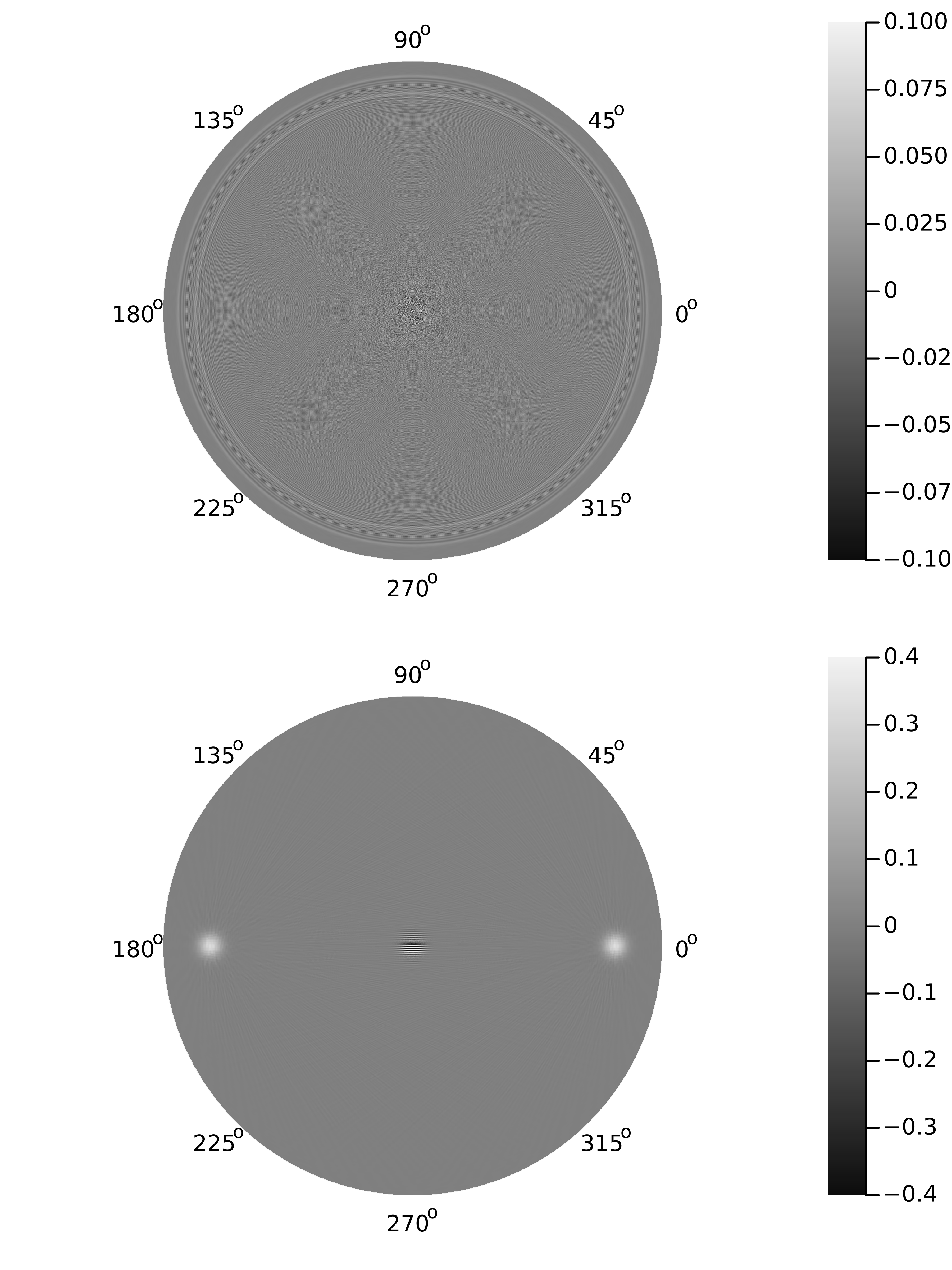
Figure 5: Wigner functions of the simulations presented in Fig. 4. Top: $\ket{\psi}\propto\ket{600}+\ket{700}$; bottom: $\ket{\psi^{\prime}}\propto\ket{\alpha}+\ket{-\alpha}$, with $\alpha=13$. To calculate these, the optimized formula in Eq. 15 was used. A window has been applied to the images for a better contrast.

For the numerical implementation we write the Wigner function in polar coordinates $W(r,\vartheta)$, with $\alpha=re^{i\vartheta}$:

$$W(r,\vartheta)=\mathrm{Re}\sum_{d=0}^{M-1}\frac{e^{i\vartheta d}}{1+\delta_{d,0}}\sum_{n=0}^{M-d-1}\lambda_{n,d}(4r^{2})\tilde{\rho}_{n,d},$$ (15)

where $\tilde{\rho}_{n,d}=(-1)^{n}\rho_{n,n+d}$ and $\lambda_{n,d}$ can be defined recursively leveraging the definition of the Laguerre polynomials, as shown in Appendix B. It is convenient to rewrite the density matrix by diagonals, reorganizing its elements for efficient memory access.

III Software package

The algorithms presented in this paper have been implemented in a Julia Bezanson et al. (2012a, 2017, b) package and a C++ package. The repositories are hosted on GitLab under the HomodyneCT group Mosco (2019a). The C++ package documentation can be found at Mosco (2019b).

The Julia package ecosystem for imaging and quantum tomography under the GitLab group HomodyneCT consists of two packages: MartaCT Mosco (2019c) and HomodyneImaging Mosco (2019d). The first one implements the tools needed for image analysis and the traditional reconstruction algorithms with FBP methods (this package is open-source and distributed under the MIT license); the second one implements all the quantum algorithms described in this paper (this package is currently closed source, so if you need access to it, please contact the authors).

The main implementation resides in the Julia package HomodyneImaging, along with the companion package MartaCT. The basic interface is defined in MartaCT, while HomodyneImaging extends it, leveraging the multiple dispatch system of the language.

Listing 1: Code example for Fig. 6.

⬇

using HomodyneImaging, QuantumOptics, IntervalSets, Plots

using MartaCT.Simulations

M = 64 # density matrix dimension

bs = FockBasis(M-1)

a = 3

norm = sqrt(2*(1+exp(-2*abs2(a))))

psi = (coherentstate(bs, a) + coherentstate(bs, -a)) / norm

rho = tensor(psi, psi’)

xs = linspace(-5..5, 600)

W = wigner(rho, xs, xs, FFTWigner())

fs = linspace(ORI(0..2pi), 300)

marg = radon(W, xs, fs, RadonSquare())

sim = SinogramHomodyneSimulation(

nsamples=1000, nblks=10, ndim=M)

rhosim, rhodiag, yerrors = simulate(sim, marg, xs, fs)

Wsim = wigner(rhosim, xs, xs, FFTWigner())

dmp = bar(0:M-1, rhodiag;

c=:red,

yerrors,

leg=:none,

lw=0,

lc=:red,

xguide="\$n\$",

guidefontsize=14,

)

wigp = heatmap(xs, xs, Wsim;

xguide="\$x\$",

yguide="\$y\$",

guidefontsize=14,

)

plot(

dmp,

wigp;

dpi=300

)

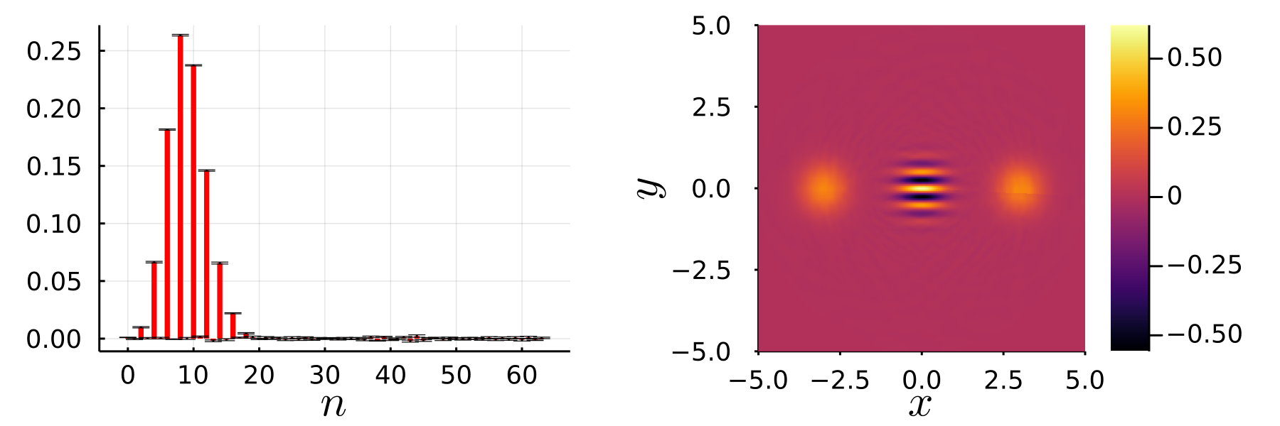
Figure 6: Example image obtained with the HomodyneImaging package representing a cat state $\ket{\psi}\propto\ket{\alpha}+\ket{-\alpha}$, with $\alpha=3$.

In order to give a sense to the reader of how MartaCT can be used, we provide an example to reconstruct a symmetric cat state $\ket{\psi}\propto\ket{\alpha}+\ket{-\alpha}$, with $\alpha=3$. The example LABEL:lst:example uses the Julia package QuantumOptics Krämer et al. (2018) to construct the quantum state. The resulting reconstruction is depicted in Fig. 6.

Let us dive in a bit in the source code of the example. First of all, in Julia one needs to import the necessary modules providing the funcionality we are going to use: this is done with the using keyword, followed by a comma-separated list of module names. We import several modules: HomodyneImaging for the HCT algorithm; QuantumOptics for the basic definitions regarding quantum states; IntervalSets which provides a nice syntax for intervals; Plots which is one of the most used plotting packages available in Julia; and finally we explicitly import MartaCT.Simulations which is a sub-module providing the definition of the simulate function which is used to perform a simulated experiment.

The parameters for this example are provided right after the imported modules: we define a variable M which is the dimension of the density matrix; the bs variable that holds the basis data for the given dimension; a the parameter of the coherent states. Then we define the state psi as a symmetric superposition of coherent states and the density matrix rho. The Wigner function W is computed with the function wigner using the algorithm FFTWigner described in this paper.

In order to perform the simulation we need to compute the marginals of the Wigner function first: this is achieved computing the Radon transform of W with radon, computing it on a square.

The simulation parameters are specified creating an object of type SinogramHomodyneSimulation, whose name recall the fact that we are providing the marginals—namely, the sinogram. The result of the simulation is stored in the variable rhosim, providing the simulated density matrix, along with the data of the diagonal and its statistical errors. With the simulated data we can compute again the Wigner function. The example is concluded by the generation of the plots shown in Fig. 6.

IV Conclusions

In conclusion, we have reviewed the homodyne tomography technique, showing how to adapt it to high-dimensional state reconstructions. We have described how this method can be implemented in practice. We gave some illustrative examples in the form of Monte Carlo simulations of the reconstruction experiments. They demonstrate the robustness of the method.

Furthermore, we present the software packages implementing the reconstruction algorithms. The main development has been focused on the Julia packages providing a new promising ecosystem for both medical imaging and quantum tomography applications.

V Acknowledgments

This work has been possible thanks to the support of the ATTRACT project “Quantum Imaging for Tomography” (QuIT) https://attract-eu.com/showroom/project/quantum-imaging-for-tomography-quit and also the Unitary Fund project https://unitary.fund/grants.html. LM acknowledges support from the U.S. Department of Energy, Office of Science, National Quantum Information Science Research Centers, Superconducting Quantum Materials and Systems Center (SQMS) under contract number DE-AC02-07CH11359.

Appendix A Review of the derivation of the tomographic formulae

The tomographic reconstruction for the homodyne detector relies on the fact that the displacement operators $D(\alpha)=e^{\alpha a^{\dagger}-\bar{\alpha}a}$ are a complete orthonormal basis for the space of operators with respect to the Hilbert–Schmidt scalar product: $\braket{A}{B}=\mathrm{Tr}[A^{\dagger}B]$. More precisely, for any linear operator $A$ one can write

$$\begin{split}A&=\frac{1}{\pi}\int_{\mathbb{C}}\mathrm{Tr}[AD^{\dagger}(\alpha)]D(\alpha)\,\mathrm{d}\mkern 0.0mu^{2}\alpha\\ &=\frac{1}{4\pi}\int_{0}^{\pi}\int_{\mathbb{R}}\mathrm{Tr}[Ae^{ikX_{\varphi}}]e^{-ikX_{\varphi}}\lvert k\rvert\,\mathrm{d}\mkern 0.0muk\mathrm{d}\mkern 0.0mu\varphi,\end{split}$$ (16)

where $\alpha$ is written in polar coordinates in the last equation: $\alpha=ike^{i\varphi}/2$, and the first integral can be taken only on the interval $[0,\pi]$ because of the symmetry $X_{\varphi+\pi}=-X_{\varphi}$. The tomographic formula is then obtained by introducing the probability $p_{\varphi}(x)={}_{\varphi}\!\braket{x}{\rho}{x}_{\varphi}$ of getting $x$ when measuring $X_{\varphi}$:

$$\braket{A}=\mathrm{Tr}[A\rho]=\frac{1}{\pi}\int_{0}^{\pi}\int_{\mathbb{R}}p_{\varphi}(x)K_{\varphi}[A](x)\,\mathrm{d}\mkern 0.0mux\mathrm{d}\mkern 0.0mu\varphi.$$ (17)

The operator $K_{\varphi}[A]$ is the so-called kernel of homodyne tomography, defined by

$$K_{\varphi}[A](x)=\frac{1}{4}\int_{\mathbb{R}}\mathrm{Tr}\left[Ae^{ik(X_{\varphi}-x)}\right]\lvert k\rvert\,\mathrm{d}\mkern 0.0muk.$$ (18)

Now, thanks to the trace in the integral, the kernel does not necessarily diverge. It is possible to classify the set operators $A$ which produce a bounded kernel D’Ariano (2002) in Eq. 17. In the simplest case considered here, the operator $A$ should be at least Hilbert–Schmidt. In particular this is the case of $\ket{n}\!\!\mkern 2.0mu\bra{m}$ which provides the matrix elements $\rho_{nm}$.

Since the first appearance D’Ariano et al. (1994) of this method there have been several attempts to simplify the expression of the tomographic formula for $\rho_{n,m}$. Let us rewrite Eq. 17 for $\rho_{n,m}$ with explicit phase dependence:

$$\rho_{n,n+d}=\frac{1}{\pi}\int_{0}^{\pi}\!\!\!\mathrm{d}\mkern 0.0mu\varphi\,e^{-id\varphi}\int_{R}\mathrm{d}\mkern 0.0mux\,p_{\varphi}(x)f_{n,n+d}(x),$$ (19)

where $f_{n,m}(x)$ are the so-called pattern functions, which are real and satisfy the symmetries:

$$f_{n,m}(x)=f_{m,n}(x),$$ (20)

$$f_{n,m}(-x)=(-1)^{n-m}f_{n,m}(x).$$ (21)

The analytical expression for the pattern functions$f_{n,m}(x)$ has been obtained by D’Ariano, Leonhardt and Paul Paul et al. (1995); D’Ariano et al. (1995); Leonhardt et al. (1995) symplifying previous derivations as follows (notation and conventions from D’ariano (1997)):

$$f_{n,m}(x)=2\sqrt{\frac{n!}{(n+d)!}}e^{-x^{2}}\cdot\phantom{x}\\ \sum_{\nu=0}^{n}\frac{(-1)^{\nu}}{\nu!}\binom{n+d}{n-\nu}(2\nu+d+1)!\cdot\phantom{x}\\ \mathrm{Re}\left[(-i)^{d}D_{-(2\nu+d+2)}(-2ix)\right],$$ (22)

where $D_{\lambda}(z)$ denotes the parabolic cylinder function. Such expression is very delicate to be used in numerical implementations for large quantum numbers.

Further simplifications were possible thanks to an insight of Richter Richter (1996) who has been able to link the tomographic formula to the regular and irregular solutions of the Schrödinger equation of the harmonic oscillator. The pattern functions are related to the solutions of the Schrödinger equations employing an Hilbert transformation. The pattern functions $f_{n,m}$ can be written as a derivative of some functions $g_{n,m}$ Leonhardt et al. (1995, 1996):

$$f_{n,m}(x)=\frac{\partial g_{n,m}}{\partial x}(x),$$ (23)

where the functions $g_{n,m}$ are obtained through a Hilbert transformation:

$$g_{n,m}(x)=\frac{\mathcal{P}}{\pi}\int_{\mathbb{R}}\frac{u_{n}(\xi)u_{m}(\xi)}{x-\xi}\,\mathrm{d}\mkern 0.0mu\xi,$$ (24)

where $\mathcal{P}$ denotes the Cauchy principal value and $u_{n}$ are the normalizable solutions of the Schrödinger equation

$$\left\lparen-\frac{1}{2}\frac{\partial^{2}}{\partial x^{2}}+\frac{x^{2}}{2}\right\rparen u_{n}(x)=\left\lparen n+\frac{1}{2}\right\rparen u_{n}(x).$$ (25)

In the same ref. Leonhardt et al. (1996), the authors were able to obtain an explicit expression for the functions $g_{n,m}$:

$$g_{n,m}(x)=u_{n}(x)v_{m}(x),\quad\text{for $m\geq n$,}$$ (26)

while for $m<n$ one can use $g_{n,m}=g_{m,n}$. Here, the functions $v_{m}$ are the irregular solutions of the Schrödinger equation, namely unnormalizable solutions continued to the complex plane:

$$\left\lparen-\frac{1}{2}\frac{\partial^{2}}{\partial z^{2}}+\frac{z^{2}}{2}\right\rparen v_{m}(z)=\left\lparen m+\frac{1}{2}\right\rparen v_{m}(z),$$ (27)

with $v_{m}(z)$ real on the real axis $z=x$.

The evaluation of the pattern functions $f_{nm}$ can be implemented efficiently on a computer by employing the factorized form

$$f_{n,m}(x)=2xu_{n}(x)v_{m}(x)-\phantom{x}\\ \sqrt{n+1}u_{n+1}(x)v_{m}(x)-\phantom{x}\\ \sqrt{m+1}u_{n}(x)v_{m+1}(x),$$ (28)

for $m\geq n$, while for $m<n$ we use the symmetry $f_{n,m}(x)=f_{m,n}(x)$. On one side, for the “regular” solutions $u_{n}(x)$ one can use the following recurrence relation:

$$\begin{cases}&u_{0}(x)=e^{-x^{2}},\\ &u_{1}(x)=2xe^{-x^{2}},\\ &u_{n}(x)=\frac{1}{\sqrt{n}}\left\lparen 2xu_{n-1}(x)-\sqrt{n-1}u_{n-2}(x)\right\rparen.\end{cases}$$ (29)

On the other side, for the irregular wavefunctions $\varphi_{m}$, we have to setup a more careful construction, as explained in Leonhardt et al. (1996). In the region given by the Bohr–Sommerfeld radius, the classically allowed region, we should employ a backward recursion instead. A safe choice for this is to consider the region

$$\lvert x\rvert<\alpha_{4k}-\frac{1}{2}\frac{1}{\sqrt[3]{\alpha_{4k}}},$$ (30)

with $\alpha_{n}=\sqrt{n+1/2}$. In this case, it is recommended to use the backward recursion as follows:

$$v_{m}(x)=\frac{1}{\sqrt{m+1}}\left\lparen 2xv_{m+1}(x)-\sqrt{m+2}v_{m+2}(x)\right\rparen,$$ (31)

with initial values obtained from a semiclassical approximation Leonhardt et al. (1996) valid for large $m$

$$v_{m}(x)=\kappa_{m}\coloneqq\frac{(8\pi)^{1/4}}{\sqrt{\alpha_{m}\sin\tau_{m}}}\sin\left\lparen\frac{1}{2}\alpha_{m}^{2}\chi_{m}+\frac{\pi}{4}\right\rparen,$$ (32)

where

$$\tau_{m}=\arccos(x/\alpha_{m}),\quad\chi_{m}=\sin(2\tau_{m})-2\tau_{m}.$$

When $x$ is outside of the region Eq. 30, one can employ the asymptotic form for $v_{m}$, which is implemented by a forward recursion Leonhardt et al. (1996):

$$\begin{cases}&v_{0}(x)=\frac{1}{x}e^{x^{2}},\\ &v_{m}(x)=\frac{\sqrt{m}}{2x}v_{m-1}(x).\end{cases}$$ (33)

Appendix B Recurrences for the Wigner function

We have seen an optimized form of the reconstruction method for the density matrix, but it may still be interesting to recover also the Wigner function. We present here two recursive methods to compute the functions $\lambda_{n,d}$, leveraging the recurrence relations of the Laguerre polynomials $L_{n}^{d}(x)$.

B.1 Method 1

Let us first recall the recursive definition of the (generalized) Laguerre polynomials Abramowitz et al. (1988):

$$\begin{aligned} &L_{0}^{d}(x)=1,\\ &L_{1}^{d}(x)=1+d-x,\\ &L_{n}^{d}(x)=a_{n,d}L_{n-1}^{d}(x)-b_{n,d}L_{n-2}^{d}(x),\\ \end{aligned}$$ (34)

with

$$a_{n,d}=\frac{2n+d-x-1}{n},\quad b_{n,d}=\frac{n+d-1}{n}.$$

We introduce the function

$$\mathcal{G}_{n}^{d}(x)=\sqrt{\frac{n!}{(n+d)!}}\mathcal{L}_{n}^{d}(x),$$ (35)

where $\mathcal{L}_{n}^{d}(x)=z(x)L_{n}^{d}(x)$ and $z(x)=\Lambda_{0}e^{-x^{2}}$, with $\Lambda_{0}=4/\pi$. The function $\lambda_{n,d}(x)$ in Eq. 15, thus, can be computed as

$$\lambda_{n,d}(x)=x^{d/2}\mathcal{G}_{n}^{d}(x).$$ (36)

In the following we will drop the dependence on the variable $x$. $\lambda_{n,d}$ can be viewed as a matrix of which only the elements $n\leq M-d-1$ have to be computed:

$$\begin{array}[]{ccccc}\square&\square&\square&\square&\square\\ \square&\square&\square&\square&\blacksquare\\ \square&\square&\square&\blacksquare&\cdot\\ \square&\square&\blacksquare&\cdot&\cdot\\ \square&\blacksquare&\cdot&\cdot&\cdot\end{array}$$

The starting point is $\lambda_{0,0}=z$, and the first 2 rows can be obtained by

$$\lambda_{0,d}=\sqrt{\frac{x}{d}}\lambda_{0,d-1},\quad\lambda_{1,d}=\frac{1+d-x}{\sqrt{d+1}}\lambda_{0,d},$$ (37)

while the first column $\lambda_{n,0}=\mathcal{L}_{n}^{0}$ is just given by the (scaled) Laguerre polynomials.

$$\begin{array}[]{ccccc}z&\sqrt{x}z&\lambda_{0,2}&\cdots&\cdots\\ (1-x)z&\frac{\sqrt{x}z}{\sqrt{2}}(2-x)&\lambda_{1,2}&\cdots&\blacksquare\\ \mathcal{L}_{2}^{0}&\square&\square&\blacksquare&\cdot\\ \vdots&\square&\blacksquare&\cdot&\cdot\\ \vdots&\blacksquare&\cdot&\cdot&\cdot\end{array}$$

At this point we can provide the general recursive formula, valid for $n\geq 2$ and $d\geq 0$ (for $d=0$ the following relation just simplifies to that of the Laguerre polynomials, so that the first column can be computed with specialized formulae):

$$\lambda_{n,d}=a^{\prime}_{n,d}\lambda_{n-1,d}-b^{\prime}_{n,d}\lambda_{n-2,d},$$ (38)

where

$$a^{\prime}_{n,d}=\frac{2n+d-x-1}{\sqrt{n(n+d)}},$$

$$b^{\prime}_{n,d}=\sqrt{\frac{(n-1)(n+d-1)}{n(n+d)}}.$$

B.2 Method 2

We can provide another implementation of the Eq. 15 computing the function $\lambda_{n,d}$ with different recurrence relations which rely on the summation property of the Laguerre polynomials $L_{n}^{d}$ which extends to the functions $\mathcal{G}_{n}^{d}(x)$:

$$L_{n}^{d}=L_{n-1}^{d}+L_{n}^{d-1}.$$ (39)

Again the starting point of the recursion is $\lambda_{0,0}=z$ and the first row is given by $\lambda_{0,d}=\sqrt{\frac{x}{d}}\lambda_{0,d-1}$, while the first column is obtained as before from $\mathcal{L}_{n}^{0}$:

$$\begin{array}[]{ccccc}z&\lambda_{0,1}&\cdots&\cdots&\cdots\\ (1-x)z&\lambda_{1,1}&\cdots&\cdots&\blacksquare\\ \mathcal{L}_{2}^{0}&\square&\square&\blacksquare&\cdot\\ \vdots&\square&\blacksquare&\cdot&\cdot\\ \vdots&\blacksquare&\cdot&\cdot&\cdot\end{array}$$

The general recursion formula, valid for $n\geq 1$ and $d\geq 1$, is now given by:

$$\lambda_{n,d}=\frac{\sqrt{n}\lambda_{n-1,d}-\sqrt{x}\lambda_{n,d-1}}{\sqrt{n+d}}.$$ (40)

With respect to the first method, in this case one needs an additional vector to store the values $\lambda_{n,d-1}$.

References

- D’Ariano and Yuen (1996) G. M. D’Ariano and H. P. Yuen, Phys. Rev. Lett. 76, 2832 (1996).
- D'Ariano et al. (2000) G. M. D'Ariano, L. Maccone, and M. G. A. Paris, Journal of Physics A: Mathematical and General 34, 93 (2000).
- D’Ariano et al. (2003) G. M. D’Ariano, M. G. A. Paris, and M. F. Sacchi, Advances in Imaging and Electron Physics 128, 206 (2003).
- D’Ariano et al. (2004) G. M. D’Ariano, M. G. Paris, and M. F. Sacchi, 2 quantum tomographic methods, in Quantum State Estimation, edited by M. Paris and J. Řeháček (Springer Berlin Heidelberg, Berlin, Heidelberg, 2004) pp. 7–58.
- D’Ariano et al. (2007) G. M. D’Ariano, L. Maccone, and M. F. Sacchi, in Quantum Information With Continuous Variables of Atoms and Light (World Scientific, 2007) pp. 141–158.
- Lutterbach and Davidovich (1997) L. G. Lutterbach and L. Davidovich, Phys. Rev. Lett. 78, 2547 (1997).
- Vogel and Risken (1989) K. Vogel and H. Risken, Phys. Rev. A 40, 2847 (1989).
- D’Ariano et al. (1994) G. M. D’Ariano, C. Macchiavello, and M. G. A. Paris, Phys. Rev. A 50, 4298 (1994).
- Paul et al. (1995) H. Paul, U. Leonhardt, and G. M. D’Ariano, Acta Physica Slovaca 45, 261 (1995).
- D’Ariano et al. (1995) G. M. D’Ariano, U. Leonhardt, and H. Paul, Phys. Rev. A 52, R1801 (1995).
- Leonhardt et al. (1995) U. Leonhardt, H. Paul, and G. M. D’Ariano, Phys. Rev. A 52, 4899 (1995).
- Rossi (2018) R. J. Rossi, Mathematical statistics: an introduction to likelihood based inference (John Wiley & Sons, 2018).
- Vlastakis et al. (2013) B. Vlastakis, G. Kirchmair, Z. Leghtas, S. E. Nigg, L. Frunzio, S. M. Girvin, M. Mirrahimi, M. H. Devoret, and R. J. Schoelkopf, Science 342, 607 (2013).
- Eichler et al. (2011) C. Eichler, D. Bozyigit, C. Lang, L. Steffen, J. Fink, and A. Wallraff, Phys. Rev. Lett. 106, 220503 (2011).
- Eichler et al. (2012) C. Eichler, D. Bozyigit, and A. Wallraff, Phys. Rev. A 86, 032106 (2012).
- Mallet et al. (2011) F. Mallet, M. A. Castellanos-Beltran, H. S. Ku, S. Glancy, E. Knill, K. D. Irwin, G. C. Hilton, L. R. Vale, and K. W. Lehnert, Phys. Rev. Lett. 106, 220502 (2011).
- Leonhardt and Munroe (1996) U. Leonhardt and M. Munroe, Phys. Rev. A 54, 3682 (1996).
- Leonhardt et al. (1996) U. Leonhardt, M. Munroe, T. Kiss, T. Richter, and M. Raymer, Optics Communications 127, 144 (1996).
- D’ariano (1997) G. M. D’ariano, Measuring quantum states, in Quantum Optics and the Spectroscopy of Solids: Concepts and Advances, edited by T. Hakioğlu and A. S. Shumovsky (Springer Netherlands, Dordrecht, 1997) pp. 175–202.
- Bezanson et al. (2012a) J. Bezanson, S. Karpinski, V. B. Shah, and A. Edelman, arXiv preprint arXiv:1209.5145 (2012a).
- Bezanson et al. (2017) J. Bezanson, A. Edelman, S. Karpinski, and V. B. Shah, SIAM Review 59, 65 (2017).
- Bezanson et al. (2012b) J. Bezanson, S. Karpinski, V. B. Shah, and A. Edelman, Julia language (2012b).
- Mosco (2019a) N. Mosco, Homodyne computed tomography (2019a).
- Mosco (2019b) N. Mosco, Hct tools (2019b).
- Mosco (2019c) N. Mosco, Marta ct (2019c).
- Mosco (2019d) N. Mosco, Homodyne imaging (2019d).
- Krämer et al. (2018) S. Krämer, D. Plankensteiner, L. Ostermann, and H. Ritsch, Computer Physics Communications 227, 109 (2018).
- D’Ariano (2002) G. M. D’Ariano, in In International School of Physics Enrico Fermi (IOS Press, 2002).
- Richter (1996) T. Richter, Physics Letters A 211, 327 (1996).
- Abramowitz et al. (1988) M. Abramowitz, I. A. Stegun, and R. H. Romer, Handbook of mathematical functions with formulas, graphs, and mathematical tables (American Association of Physics Teachers, 1988).