Relaxed Magnetohydrodynamics with Ideal Ohm’s Law Constraint (arxiv v2)

Abstract

The gap between a recently developed dynamical version of relaxed magnetohydrodynamics (RxMHD) and ideal MHD (IMHD) is bridged by approximating the zero-resistivity “Ideal” Ohm’s Law (IOL) constraint using an augmented Lagrangian method borrowed from optimization theory. The augmentation combines a pointwise vector Lagrange multiplier method and global penalty function method and can be used either for iterative enforcement of the IOL to arbitrary accuracy, or for constructing a continuous sequence of magnetofluid dynamics models running between RxMHD (no IOL) and weak IMHD (IOL almost everywhere). This is illustrated by deriving dispersion relations for linear waves on an MHD equilibrium.

¹Mathematical Sciences Institute, The Australian National University, Canberra, ACT 2601, Australia

1 Introduction

1.1 Basics

In this paper choosing constraint equations is central to our approach to developing new fluid models. The concept of a constraint equation occurs in both the variational approach to classical mechanics [see e.g. Goldstein (1980)] and optimization theory [see e.g. Nocedal & Wright (2006)]. While both traditionally treat finite-dimensional systems, the language and techniques of these fields can also help in understanding the infinite-dimensional dynamics of non-dissipative continuous media. In the following we shall distinguish between a hard constraint, i.e. one that is enforced exactly, a soft constraint, one that is enforced only approximately, and a weak version of a hard constraint, one that is enforced as the limiting case of a sequence of soft constraints (formulating such a method being the goal of this work, which it is hoped will lead to a physical regularization of MHD that allows reconnection).

We also distinguish between microscopic, i.e. acting within each fluid element or infinitesimal parcel of fluid, and macroscopic constraints, i.e. global within a spatial domain $\Omega$ of the fluid (or subdomain if the system is partitioned into multiple regions).

The mathematical model we seek to regularize is Ideal MHD (IMHD), a special case in the general field of magnetohydrodynamics (MHD). In the general, resistive case Ohm’s Law is $\bm{E}^{\prime}=\eta\bm{j}$, where

$$\bm{E}^{\prime}[\bm{u}]\stackrel{{\scriptstyle\text{def}}}{{=}}\bm{E}+\bm{u}\bm{\times}\bm{B}$$ (1)

is the electric field observed in the local frame of each fluid element, $\bm{E}$ being the electric field in the lab frame. These elements are advected in the fluid velocity field $\bm{u}(\bm{x},t)$ (i.e. $\dot{\bm{x}}=\bm{u}$ at each spatial point $\bm{x}$ and time $t$). Also $\bm{B}(\bm{x},t)$ is the magnetic field, $\eta$ is the resistivity and $\bm{j(\bm{x},t)}$ is the electric current density (N.B. $\bm{j}=\bm{\nabla}\bm{\times}\bm{B}/\upmu_{0}$ in standard non-relativistic MHD, where $\upmu_{0}$ is the vacuum permeability constant used in SI electromagnetic units). We have exhibited $\bm{u}$ as an explicit argument for use later in the paper, while leaving dependencies on $\bm{x},t,\bm{E,}$ and $\bm{B}$ implicit.

To get IMHD, set $\eta=0$ so that $\bm{E}^{\prime}=0$, giving what is often called the Ideal Ohm’s Law (IOL):

$$\bm{E}+\bm{u}\bm{\times}\bm{B}=0\;.$$ (2)

While $\bm{E}$ is not usually explicit in the IMHD equations, this is only because it is eliminated between (2), after taking the curl of both sides, and the Maxwell–Faraday induction equation

$$\bm{\nabla}\bm{\times}\bm{E}=-\partial_{t}\bm{B}\;,$$ (3)

to give the IMHD magnetic-field propagation equation

$$\partial_{t}\bm{B}+\bm{\nabla}\bm{\times}(\bm{u}\bm{\times}\bm{B})=0\;.$$ (4)

With the “pre Maxwell” Ampère’s Law $\bm{j}=\bm{\nabla}\bm{\times}\bm{B}/\upmu_{0}$ and $\bm{\nabla\cdot}\bm{B}=0$, the Maxwell-Faraday equation (3) plays the important role of preserving Galilean invariance [Hosking & Dewar (2015, Sec. 5.4); Webb & Anco (2019)], independent of whether or not the IOL equation is enforced. Thus we shall retain it in the following development of a dynamical relaxation theory.

Equation (3) can be viewed as a holonomic constraint on $\bm{E}$, and likewise $\bm{\nabla\cdot}\bm{B}=0$ is a holonomic constraint on $\bm{B}$, i.e. we can remove these constraints from consideration by expressing the constrained variables in terms of fewer unconstrained variables. Here these are the vector and scalar potentials $\bm{A}$ and $\Phi$, respectively, in terms of which

$$\bm{B} =\bm{\nabla}\bm{\times}\bm{A}\;,$$ (5)

$$\bm{E} =-\partial_{t}\bm{A}-\bm{\nabla}\Phi\;.$$ (6)

These imply $\bm{\nabla\cdot}\bm{B}=0$ and also (3), as is easily seen by calculating $\bm{\nabla}\bm{\times}\bm{E}$.

We restrict the choice of gauge to be such that $\Phi$ is a spatially single-valued potential and such that $\partial_{t}\bm{A}=0$ in equilibrium cases in a frame (the LAB frame) where $\partial_{t}\,\cdot=0$, so $\bm{A}$ has no effect on $\bm{E}$ in that static case. Of course the vector potential still does play an explicit role in describing plasma equilibria because the magnetic flux threading a loop is $\oint\bm{A}\bm{\cdot}\mathrm{d}\bm{l}$. Dynamically, only $\partial_{t}\bm{A}$ contributes to inductive e.m.f.s $\oint\bm{E}\bm{\cdot}\mathrm{d}\bm{l}$ around closed loops. In our case, we assume e.m.f.s are zero around any loop on the boundary $\partial\Omega$ — the trapped-flux boundary condition of RxMHD [see Appendix B of Dewar et al. (2015)]. Aside from this restriction, there is still considerable gauge freedom in $\bm{A}$. If we choose Coulomb gauge, $\bm{\nabla\cdot}\bm{A}=0$, the potential representation is an example of the Helmholtz decomposition of an arbitrary vector field into the sum of curl-free and divergence-free vector fields, but we shall not make this gauge choice except in Sections 5.5 and 6 — we shall treat the magnetic helicity term carefully in our general derivation of the conservation form momentum equation in order to make it gauge invariant.

1.2 Methodology: Variational principles and Euler–Lagrange equations

In mechanics and optimization theory there are objective functions whose extrema — maxima, minima and saddle points — are given by Euler–Lagrange (EL) equations, which are found by setting first derivatives of these functions to zero. In mechanics such functions are Hamiltonians whose extrema give stable or unstable equilibria, or actions, time integrals of Lagrangians, whose extrema give physical time evolution equations (Hamilton’s Principle).

The main aim of this paper is to use an infinite-dimensional generalization of Hamilton’s Principle in which partial derivatives are replaced by functional derivatives [see e.g. Morrison (1998)] of action integrals incorporating the IOL constraint, and also global entropy, magnetic-helicity and cross-helicity constraints. These functional derivatives are with respect to the basic physical fields, e.g. $\Phi$, $\bm{A}$, $\bm{u}$, etc., describing the state of the system and are set to zero to find a set of Euler–Lagrange equations which together are sufficient to describe the dynamics of the system. For brevity we shall refer e.g. to the equation found by setting the functional derivative with respect to $\Phi$ as the “$\delta\Phi$-EL equation”.

1.3 Relaxation

See Appendix A for a brief history of the variational approach to finding relaxed plasma equilibrium states by minimizing the IMHD energy functional using one or more IMHD invariants as global constraints. This construction implies immediately that such relaxed magnetostatic states are a special subset of all possible IMHD equilibria, most of which, being of higher energy, are likely to be more unstable than relaxed states.

In this paper we instead seek to find a time-dependent variational formulation for relaxed plasma systems going through a dynamical phase as they transition from one equilibrium state to another (e.g. due to boundary deformations). Thus, instead of minimizing energy, we use Hamilton’s variational Principle, widely regarded as the most fundamental principal in all mathematical physics, from general relativity through classical mechanics to quantum field theories (for instance connecting symmetries and conservation laws by Noether’s theorem). As we are attempting to establish a new classical field theory related to, but different from, ideal magnetohydrodynamics (IMHD), it is appropriate to seek new magnetofluid models by modifying the IMHD Hamilton’s Principle.

Following this precept, Dewar et al. (2020) derived a new dynamical magnetofluid model, Relaxed MagnetoHydroDynamics (RxMHD), from Hamilton’s Action Principle using a phase-space version of the magnetofluid Lagrangian with a noncanonical momentum field $\bm{u},$ physically identified as the lab-frame mass-flow velocity, and a kinematically constrained velocity field $\bm{v}$ (the fluid velocity relative to a magnetic-field-aligned flow). The resulting Euler–Lagrange equations generalize from statics to dynamics the usual relaxation-by-energy-minimization concept developed by Taylor (1986) for flowless plasma equilibria, and its generalization to equilibria with steady flow by various authors: Finn & Antonsen (1983); Hameiri (1998); Vladimirov et al. (1999); Hameiri (2014); Dennis et al. (2014b). These generalized Taylor equilibria were shown by Dewar et al. (2020) to be consistent with RxMHD when time derivatives are set to zero. However, specific cases of equilibria with flows not aligned with the magnetic field have been limited to axisymmetric equilibria, whereas in this paper we aim to treat more general, non-axisymmetric (3-D) equilibria with flow, as well as time-dependent problems such as the calculation of the spectrum of normal modes of oscillation of 3-D relaxed equilibria.

The advection equation for $\bm{B}$, (4), implies the “frozen-in flux constraint”, which, as discussed by Newcomb (1958), preserves the topology of magnetic field lines. This prevents field-line breaking and reconnection from forming new structures, such as magnetic islands, and this frustration of topological changes leads to singularities developing as time tends toward infinity Grad (1967).

Though in this paper we proceed in a formal way by simply inserting constancy constraints of selected IMHD invariants as postulates, historically the heuristic assumption motivating relaxation theory is that, if it would be energetically favourable to do so, and on a long enough timescale, “nature will find a way” for reconnection to occur, either due to the magnifying effect of large gradients on small but finite resistivity at singularities, or through “anomalous” phenomena such as turbulence. Thus in the RxMHD of Dewar et al. (2020) the continuum of local frozen-in flux constraints is replaced by only two constraints involving $\bm{B}$, the two global IMHD invariants magnetic helicity and cross helicity.

However, as will be argued in Subsection 3.2, there is reason to believe that, for general three-dimensional equilibria with non-integrable magnetic field dynamics, imposing (2) as a hard constraint would lead to an ill-posed variational principle with no smooth extremum. In this case we regularize the problem by approaching an IOL-constrained state through a sequence of softly constrained states where the IOL constraint is not exactly satisfied.

For a dynamical relaxed MHD theory to be fully satisfactory we require it to be well-posed mathematically and desire it to agree with ideal MHD in two cases: (i) on the boundary $\partial\Omega(t)$, because MRxMHD interfaces are regarded as arbitrarily thin sheets of IMHD fluid; and (ii) in an equilibrium state with steady flow, when one imagines any transient non-ideal behaviour to have died away, justifying the Principle of IMHD-Equilibrium Consistency [Dewar et al. (2020)].

This Consistency Principle was satisfied by the one flowing equilibrium test case Dewar et al. (2020) looked at using their RxMHD formulation, the rigidly rotating axisymmetric steady-flow equilibrium. However RxMHD does not enforce the IOL constraint (2), so there is no reason to believe that ideal consistency would necessarily apply to more general relaxed equilibria. [Indeed, Dewar et al. (2020) showed that small dynamical perturbations about an equilibrium exhibited no tendency to preserve the IOL constraint.]

Specifically, we are interested in non-axisymmetric relaxed steady-flow toroidal equilibria such as may occur in stellarators. The elliptic nature of RxMHD (when flows are small) makes it reasonable to assume that smooth solutions of the RxMHD equations exist for such equilibria. We argue in Subsection 3.2 that, generically, magnetic field and fluid flow lines on these smooth RxMHD solutions will be chaotic so their ergodic properties will exhibit complexity on all scales.

While RxMHD offers no impediment to the formation of such fractal structure [one of the principal motivations for the develoment of the SPEC code, Hudson et al. (2012)] the same is not true for IMHD where the topological constraints arising from its frozen-in-flux properties (see above) force the formation of singularities. The ability of the SPEC equilibrium code to study difficult physical problems [Qu et al. (2020)], and subtle fundamental problems involving chaos [Qu et al. (2021)], motivates our current endeavour to extend the RxMHD formalism on which it is based to make it closer to IMHD but to retain sufficient topological relaxation to allow magnetic island formation and chaos, thus allowing further extension of SPEC to hande time-dependent problems in three-dimensional geometries.

1.4 Background flow

We define a fully relaxed RxMHD equilibrium as one where the electrostatic potential $\Phi$ has relaxed to a constant value throughout a volume $\Omega$, so $\bm{E}=0$. As Finn & Antonsen (1983) recognized, this would occur in the extreme case where magnetic field lines fill $\Omega$ ergodically, because dotting both sides of (2) with $\bm{B}$ gives the derivative along $\bm{B}$ as $\bm{B}\bm{\cdot}\bm{\nabla}\Phi=0$. As we shall see, constant $\Phi$ implies purely parallel flow, $\bm{u}=\bm{u}_{\parallel}$, whose magnitude is constrained by the steady-flow continuity equation $\bm{\nabla\cdot}[(\rho/B)\bm{B}u_{\parallel}]=\bm{B}\bm{\cdot}\bm{\nabla}(\rho u_{\parallel}/B)=0$, where $\rho$ is mass density. For consistency again with the (unachievable) fully ergodic limit, we define fully relaxed parallel flow as such that $\rho u_{\parallel}/B={\mathrm{const}}$. We denote this special parallel flow velocity as

$$\bm{u}^{\rm Rx}\stackrel{{\scriptstyle\text{def}}}{{=}}\frac{\nu_{\Omega}\bm{B}}{\upmu_{0}\rho}\;,$$ (7)

where $\nu_{\Omega}$ is a constant throughout $\Omega$ — its significance in the RxMHD formalism is explained below:

In the variational $\bm{u},\!\bm{v}$ dynamical relaxation formalism of Dewar et al. (2020), EL equations for $\bm{u}$, $\bm{v}$, $\bm{B}$ and pressure $p$ are derived variationally from Hamilton’s Principle, while the mass continuity equation is built in as a holonomic constraint. The fully relaxed flow $\bm{u}^{\rm Rx}$ occurs in these EL equations, with $\nu_{\Omega}$ arising as the Lagrange multiplier for the magnetic-helicity constraint in the phase-space Lagrangian. Specifically, the EL equation arising from free variations of $\bm{u}$ is

$$\bm{u}=\bm{u}^{\rm Rx}+\bm{v}\;,$$ (8)

so $\bm{v}$ is the relative flow, the fluid velocity relative to the fully relaxed flow velocity $\bm{u}^{\rm Rx}$.

Noting from (7) that $\bm{\nabla\cdot}(\rho\bm{u}^{\rm Rx})=0$, we see that $\bm{\nabla\cdot}(\rho\bm{u})=\bm{\nabla\cdot}(\rho\bm{v})$. Thus the continuity equation holds for both $\bm{u}$ and $\bm{v}$, i.e. both flows are microscopically mass-conserving. Also, $\bm{u}\bm{\times}\bm{B}=\bm{v}\bm{\times}\bm{B}$, so $\bm{E}^{\prime}[\bm{u}]=\bm{E}^{\prime}[\bm{v}]$. In order to preserve (8) in the variational formulation (see later), the version of the IOL constraint we shall be using in the body of this paper is $\bm{E}^{\prime}[\bm{v}]=0$, which becomes equivalent to $\bm{E}^{\prime}[\bm{u}]=0$ only after the Euler–Lagrange equations are derived.

1.5 Domains and boundaries

For most purposes in this paper it is sufficient to restrict attention to plasma within a single domain $\Omega(t)$ that is closed, of genus at least 1, and whose boundary $\partial\Omega(t)$ is smooth, gapless, perfectly conducting and time-dependent. However we note this is part of a larger project, the development of Multiregion Relaxed MHD (MRxMHD) Dewar et al. (2015), in which $\Omega$ is but a subregion of a larger plasma region, partitioned into multiple relaxation domains physically separated by moving interfaces. As $\partial\Omega(t)$ is the union of the inward-facing sides of the interfaces $\Omega(t)$ shares with its neighbours, it transmits external forcing to the restricted subsystem within $\Omega(t)$ and imparts equal and opposite reaction forces on the neighbouring subdomains.

We take the interfaces to be perfectly flexible and impervious to mass and heat transport. We also take them to be impervious to magnetic flux like a superconductor, implying the tangentiality condition

$$\bm{n}\bm{\cdot}\bm{B}=0\>\>\text{on}\>\partial\Omega\;,$$ (9)

where $\bm{B}\stackrel{{\scriptstyle\text{def}}}{{=}}\bm{\nabla}\bm{\times}\bm{A}$ is the magnetic field and $\bm{n}$ is a unit normal at each point on $\partial\Omega$ (here and henceforth leaving the argument $t$ implicit in $\Omega$, $\bm{n}$ etc.). Also, to conserve magnetic fluxes trapped within $\Omega$, loop integrals of the vector potential $\bm{A}$ within the interfaces must be conserved [see e.g. Dewar et al. (2015)].

1.6 Layout of this paper

The phase-space Lagrangian variational approach to deriving ideal MHD equations is briefly reviewed in Section 2, then some general implications of the IOL when it is a hard constraint\ are discussed in Section 3 including speculations in Subsection  3.2 on the implications of chaos and ergodic theory on flows in three-dimensional systems, in Subsection 3.1 the $\bm{E}\bm{\times}\bm{B}$ drift is derived.

In Section 4 the adaptation of the augmented Lagrangian penalty function method from optimization theory to the physical purpose of approximating the IOL constraint is discussed as a softly constrained optimization problem in Subsction 4.1.1, and the specific Lagrangian density constraint term for this method is given in Subsection 4.1. The entropy, magnetic helicity and cross-helicity conservation constraints used in Relaxed MHD theory are discussed in Subsection 4.2, and the complete phase space Lagrangian to be used in this paper is constructed in Subsection 4.3.

In Section 5 the Euler–Lagrange equations, including an equation of motion in momentum conservation form, are derived formally in Subsection 5.1, and in specific forms in Subsections 5.2–5.7 where the IOL constraint term provides new contributions that vanish only when the constraint is satisfied. In addition to the momentum equation form, an equation of motion in Bernoulli form is derived. A physical interpretation of the Lagrange multiplier for the IOL constraint in terms of a polarization field is also mentioned.

Section 6 illustrates the implementaton of the augmented Lagrangian method for linear waves propagating on an IOL-compliant equilibrium in the WKB approximation. A continuous family of dispersion relations for wave residuals $\widetilde{\bm{C}}$ ranging from zero in the IMHD case to its value in the RxMHD case, where it is the perturbed Lagrange multiplier $\widetilde{\bm{\lambda}}$ that is set to zero.

The Conclusion, Section 7, briefly summarizes what has been achieved in this paper and what more needs to be done. More detail on derivations of equations is available as online Supplementary Material in an unabridged version of this paper.

A brief historical overview of MHD relaxation theory is given in Appendix A and some useful vector and dyadic calculus identities are derived in Appendix B, in particular the little-known identity (139), which is crucial for getting the general form of the momentum equation (54) into a general conservation form, (57).

2 Ideal MHD in phase space

The mathematical foundation on which our dynamical relaxation formalism is built is a noncanical form (which we call the $\bm{u}$, $\bm{v}$ picture) of the canonical MHD Hamiltonian, and a Phase-Space Lagrangian (PSL). Here we review how Hamilton’s action principle leads to IMHD when microscopic constraints on entropy and magnetic flux are applied. Later we show how RxMHD arises when these are replaced by global constraints using the same PSL formalism.

Both ideal and relaxed MHD starts from the canonical MHD Hamiltonian

$$H^{{\rm MHD}}[\bm{x},\bm{\pi},t] =\int_{\Omega}\mathcal{H^{{\rm MHD}}}\,\mathrm{d}V\;,$$

$$\text{with}\>\>\mathcal{H^{{\rm MHD}}}(\bm{x},\bm{\pi},t) \stackrel{{\scriptstyle\text{def}}}{{=}}\frac{\bm{\pi}^{2}}{2\rho}+\frac{p}{\gamma-1}+\frac{B^{2}}{2\upmu_{0}}\;,$$ (10)

where $\bm{\pi}\left(\bm{x},t\right)$ is the canonical momentum density, the analogue of $p$ in finite-dimensional classical dynamics.

The analogue of $q$ is not $\bm{x}$ the Eulerian independent variable but $\bm{r}$, the Lagrangian position with respect to a given reference frame. We do not make this explicit as we shall always work in the Eulerian picture, but the Lagrangian picture in the background does manifest in interpreting variations. [This is discussed in more detail by Dewar et al. (2020).] For instance, the analogue of the variation $\delta q$ at fixed $t$ is $\Delta\bm{x}=\bm{\xi}(\bm{x},t)$, the Lagrangian fluid displacement in Eulerian representation, and the analogue of the variation $\dot{q}\,\delta t$ is $\bm{v}(\bm{x},t)\,\delta t$, which we shall refer to as the Lagrangian velocity field (not always the same as the Eulerian velocity $\bm{u}$). Both ideal and RxMHD also use the constrained kinematic variation Newcomb (1962),

$$\delta\bm{v}=\partial_{t}\bm{\xi}+\bm{v}\bm{\cdot}\bm{\nabla}\bm{\xi}-\bm{\xi}\bm{\cdot}\bm{\nabla}\bm{v}\;.$$ (11)

They also use the mass density variation

$$\delta\rho=-\bm{\nabla\cdot}(\rho\,\bm{\xi})=-\rho\bm{\nabla\cdot}\bm{\xi}-\bm{\xi}\bm{\cdot}\bm{\nabla}\rho\;,$$ (12)

which is an expression of the microscopic conservation of mass and can be found by integrating the perturbed continuity equation

$$\partial_{t}\rho+\bm{\nabla\cdot}(\rho\bm{v})=0\>\>\Leftrightarrow\>\>\frac{\mathrm{d}\rho}{\mathrm{d}t}=-\rho\bm{\nabla\cdot}\bm{v}$$ (13)

along varied Lagrangian trajectories $\bm{r}(t|\bm{x}_{0})$ [Frieman & Rotenberg (1960)] and expressing this Lagrangian variation in the Eulerian picture [Newcomb (1962)].

Instead of seeking a Poisson bracket to get phase-space dynamics from $H$ [see e.g. Morrison (1998)], we instead work directly with the canonical phase-space Lagrangian (PSL) density $\mathcal{L^{{\rm MHD}}}$,

$$L_{{\rm ph}}^{{\rm MHD}}[\bm{x},\bm{v},\bm{\pi}] =\int_{\Omega}\!\!\left[\bm{\pi}\bm{\cdot}\bm{v}-\mathcal{H^{{\rm MHD}}}(\bm{x},\bm{\pi},t)\right]\,\mathrm{d}V\;,$$

$$\stackrel{{\scriptstyle\text{def}}}{{=}}\int_{\Omega}\!\!\,\mathcal{L^{{\rm MHD}}}(\bm{x},\bm{\pi},t)\,\mathrm{d}V$$

$$=\int_{\Omega}\!\!\left(\bm{\pi}\bm{\cdot}\bm{v}-\frac{\bm{\pi}^{2}}{2\rho}-\frac{p}{\gamma-1}-\frac{B^{2}}{2\upmu_{0}}\right)\,\mathrm{d}V\;,$$ (14)

and the corresponding canonical phase-space action,

$$\mathscr{S_{{\rm ph}}^{{\rm MHD}}}\stackrel{{\scriptstyle\text{def}}}{{=}}\iint_{\Omega}\!\!\mathcal{L^{{\rm MHD}}}\,\mathrm{d}V\mathrm{d}t$$ (15)

as the primary tools, deriving Euler–Lagrange (EL) equations from Hamilton’s Principle of stationary action,

$$\delta\mathscr{S_{{\rm ph}}^{{\rm MHD}}}=0\;,$$ (16)

varying phase space paths under appropriate constraints.

We have used the subscript notation $\cdot_{{\rm ph}}$ on the Lagrangian $L_{{\rm ph}}$ and the action $\mathscr{S}_{{\rm ph}}$ to make it clear the PSL defined in (14) is fundamentally different from the more usual configuration space Lagrangian and action. This is because, in (15), $\bm{\pi}$ is now regarded as freely variable, so the dimensionality of the space of allowed variations is doubled in the phase-space action principle.

For instance, varying $\bm{\pi}$ in (14) gives the $\delta\bm{\pi}$-EL equation $\delta\mathscr{S}_{{\rm ph}}/\delta\bm{\pi}=\bm{v}-\bm{\pi}/\rho=0$, i.e., multiplying by $\rho$, the analogue of $p=m\dot{q}$ is seen to be $\bm{\pi}=\rho\bm{v}$, as expected. Likewise, using the microscopic holonomic constraints of entropy and flux, $\delta p=-\gamma p\bm{\nabla\cdot}\bm{\xi}-\bm{\xi}\bm{\cdot}\bm{\nabla}p$ and $\delta\bm{B}=\bm{\nabla}\bm{\times}(\bm{\xi}\bm{\times}\bm{B})$, respectively, one can verify that the Euler–Lagrange equation arising from Lagrange-varying $\bm{x}$ (i.e. varying $\bm{\xi}$) is just the IMHD equation of motion.

However, as it is not customary in fluid mechanics to work with canonical momenta, we follow Burby (2017) in exploiting the freedom afforded by the PSL to work with a velocity-like phase-space variable $\bm{u}$, obtained by the noncanonical change of variable $\bm{\pi}=\rho\bm{u}$. Then the canonical Hamiltonian density (10) becomes the noncanonical Hamiltonian density

$$\mathcal{H}_{{\rm nc}}^{{\rm MHD}}(\bm{x},\bm{u},t) =\frac{\rho\bm{u}^{2}}{2}+\frac{p}{\gamma-1}+\frac{B^{2}}{2\upmu_{0}}\;,$$ (17)

and the PSL density in noncanonical form becomes, from (14),

$$\mathcal{L}_{{\rm nc}}^{{\rm MHD}}(\bm{x},\bm{u},\bm{v},t) \stackrel{{\scriptstyle\text{def}}}{{=}}\rho\bm{u}\bm{\cdot}\bm{v}-\mathcal{H}_{{\rm nc}}^{{\rm MHD}}(\bm{x},\bm{u},t)$$

$$=\rho\bm{u}\bm{\cdot}\bm{v}-\frac{\rho\bm{u}^{2}}{2}-\frac{p}{\gamma-1}-\frac{B^{2}}{2\upmu_{0}}\;.$$ (18)

As neither $p$ nor $\bm{B}$ depends on $\bm{u}$, the $\delta\bm{u}$-EL equation is $\delta\mathscr{S}_{{\rm ph}}^{{\rm MHD}}/\delta\bm{u}=\rho\bm{v}-\rho\bm{u}=0$, i.e. in IMHD we have $\bm{v}=\bm{u}$. The IMHD equation of motion, which can be written in conservation form as

$$\partial_{t}(\rho\bm{u})+\bm{\nabla\cdot}\bm{\mathsf{T}}_{{\rm{\rm MHD}}}=0\;,$$ (19)

where

$$\bm{\mathsf{T}}_{{\rm{\rm MHD}}}\stackrel{{\scriptstyle\text{def}}}{{=}}\rho\bm{u}\bm{u}+\left(p+\frac{B^{2}}{2\upmu_{0}}\right)\bm{\mathsf{I}}-\frac{\bm{B}\bm{B}}{\upmu_{0}}\;,$$ (20)

follows as it does for the $\bm{\xi}$-EL equation in the canonical form.

It will shown below that an isothermal version of IMHD can be derived by replacing the holonomic variational constraint $\delta p=-\gamma p\bm{\nabla\cdot}\bm{\xi}-\bm{\xi}\bm{\cdot}\bm{\nabla}p$ with a global entropy conservation constraint, giving thermal relaxation, a more realistic model for hot plasmas than the microscopic entropy constraints implied by $\delta p=-\gamma p\bm{\nabla\cdot}\bm{\xi}-\bm{\xi}\bm{\cdot}\bm{\nabla}p$.

3 Implications of the IOL constraint

In this section we examine consequences of applying the IOL constraint (2) in the form (see Subsection 1.4) $\bm{E}^{\prime}[\bm{v}]=0$, which can be written $-\bm{E}=\bm{v}\bm{\times}\bm{B}$ or $\partial_{t}\bm{A}+\bm{\nabla}\Phi=\bm{v}\bm{\times}\bm{B}$.

3.1 $\bm{E}\bm{\times}\bm{B}$ drift

As $\bm{E}^{\prime}=\bm{E}+\bm{v}\bm{\times}\bm{B}$ we have the two identities

$$\bm{B}\bm{\times}\bm{E}^{\prime} =-\bm{E}\bm{\times}\bm{B}+(B^{2}\bm{\mathsf{I}}-\bm{B}\bm{B})\bm{\cdot}\bm{v}\;,$$ (21)

$$\text{and}\quad\bm{v}\bm{\times}\bm{E}^{\prime} =-\bm{E}\bm{\times}\bm{v}-(v^{2}\bm{\mathsf{I}}-\bm{v}\bm{v})\bm{\cdot}\bm{B}\;.$$ (22)

Equation (21) leads to a decomposition of the relative fluid flow into a component $v_{\parallel}$ tangential to $\bm{B}$ at $\bm{x}$, and a component $\bm{v}_{\perp}$, its projection onto the plane transverse to $\bm{B}$, the “$\bm{E}\bm{\times}\bm{B}$ drift,”

$$\bm{v}_{\perp}=\frac{\bm{E}_{\perp}\bm{\times}\bm{B}}{B^{2}}\;.$$ (23)

It is usually safe to assume $B^{2}\neq 0$ anywhere in toroidally confined plasmas, so the representation (23) generally applies everywhere, and to both equilibrium and dynamic ES MHD cases.

3.2 The equilibrium ergodicity problem

Resolving the IOL onto the vectors $\bm{B}$ and $\bm{v}$ (or $\bm{u}$) eliminates the $\bm{v}\bm{\times}\bm{B}$ term, so in equilibrium, when $\partial_{t}\bm{A}=0$ these components of the IOL imply

$$\bm{B}\bm{\cdot}\bm{\nabla}\Phi =0\;,$$ (24)

$$\bm{u}\bm{\cdot}\bm{\nabla}\Phi =0\;.$$ (25)

This means $\Phi={\mathrm{const}}$ on stream lines as well as magnetic field lines. As a consequence, level sets of $\Phi$ are invariant under magnetic and fluid flow. For instance, if $\Phi$ has smoothly nested level surfaces in a region then both $\bm{u}$ and $\bm{B}$ lie in the local tangent plane at each point on each isopotential surface — the magnetic and fluid flows are both locally integrable.

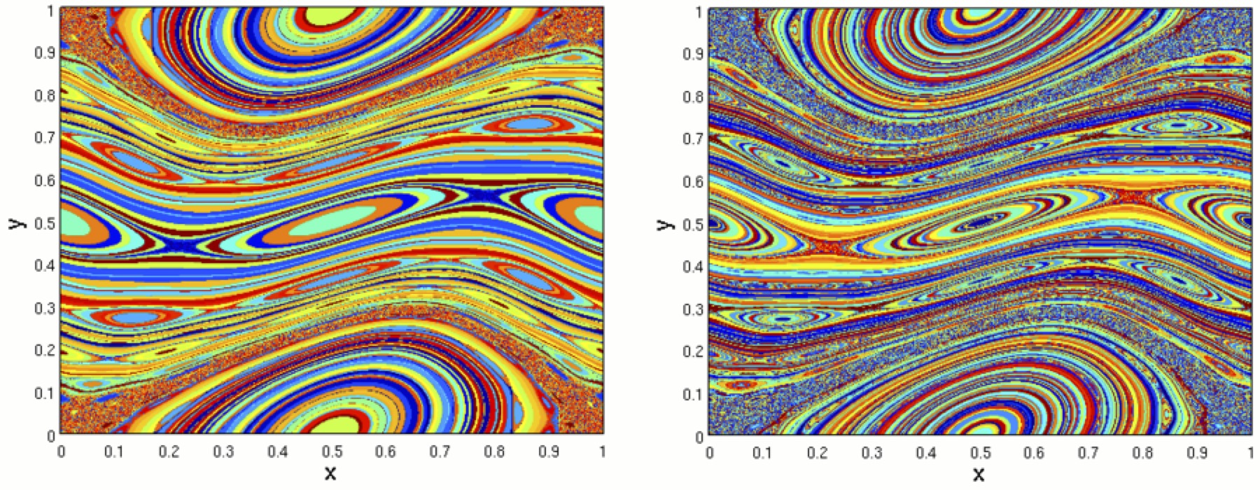
Figure 1: Ergodic partition of iterates of the standard map as depicted in Fig. 11 of Levnajić & Mezić (2010). (Reprinted with permission from Chaos.)

In the opposite extreme, Finn & Antonsen (1983) [after Eq. (29)] conclude from the constancy of $\Phi$ along a field line that “if the turbulent relaxation has ergodic field lines throughout the plasma volume,” then $\bm{\nabla}\Phi=0$, which implies that $\bm{u}\bm{\times}\bm{B}=0$ — the fluid flows along magnetic field lines. As already mentioned, we call such field-aligned steady flows fully relaxed equilibria (though the converse does not apply — field-aligned flows can be integrable).

However, field-aligned flow equilibria exclude many applications of physical interest — in particular tokamaks with strong toroidal flow. For such axisymmetric equilibria Dewar et al. (2020) show RxMHD can give the same axisymmetric relaxed solutions with cross-field flow as found by Finn & Antonsen (1983) and Hameiri (1983), but without needing the angular momentum constraint used by these authors.

Unlike Finn & Antonsen (1983) we are not appealing to turbulence to justify relaxation, but, in fully three dimensional (3-D) plasmas, we may be able to appeal to the existence of chaotic magnetic field and stream lines. However “chaotic” is not the same as “ergodic” — while chaotic flows do involve ergodicity, this is in an infinitely complicated way, visualized in Figure 1] in terms of the fractal ergodic partition of [Mezić & Wiggins (1999); Levnajić & Mezić (2010). (This figure is generated for an iterated area-preserving map, but magnetic field-line flows being flux preserving, the magnetic field-line return map of a Poincaré section onto itself in a magnetic containment device is similar.)

A similar problem involving chaos and ergodicity arises in magnetohydrostatics, Hudson et al. (2012), where the equilibrium condition $\bm{\nabla}p=\bm{j}\bm{\times}\bm{B}$ implies $\bm{B}\bm{\cdot}\bm{\nabla}p=0$, analogously to (24) for $\Phi$, so the fractal ergodic partition for field-line flow is as relevant to the pressure $p$ as it is for the potential $\Phi$. In their MRxMHD equilibrium code Hudson et al. (2012) solved the puzzle posed by Grad (1967) (i.e. how to formulate the three-dimensional IMHD equilibrium problem so as to avoid a “pathological” pressure profile) by using a much simpler ergodic partition obtained by aggregating contiguous elements of the fractal ergodic partition into a finite number of constant-pressure “relaxation regions” $\Omega_{i}$, with pressure changing (discontinuously) only across the interfaces between the $\Omega_{i}$s. The code was thus named the Stepped Presssure Equilibrium Code (SPEC).

3.2.1 Continuity of Electrostatic Potential

One might think that an analogous “stepped potential equilibrium” could provide a solution to the problem of finding a non-trivial but tractable solution of $\bm{\nabla}_{\parallel}\Phi\stackrel{{\scriptstyle\text{def}}}{{=}}(\bm{B}/B)\bm{\cdot}\bm{\nabla}\Phi=0$ in a chaotic magnetic-field-line flow. Unfortunately however we must restrict $\bm{\nabla}_{\perp}\Phi\stackrel{{\scriptstyle\text{def}}}{{=}}(\bm{\mathsf{I}}-\bm{B}\bm{B}/B^{2})\bm{\cdot}\bm{\nabla}\Phi$ to square-integrable functions in order to keep the $\bm{E}\bm{\times}\bm{B}$ drift (23) from acquiring a $\delta$-function component.

This rules out having steps in $\Phi$ because $\delta$-functions are not square integrable, so stepped potentials would make the kinetic energy integral infinite. However, this does not necessarily imply $\Phi$ is constant in weakly chaotic regions with a finite measure of KAM surfaces — perhaps weak KAM theory [see e.g. Fathi (2009)] would allow fractal potential profiles having finite kinetic energy associated with them.

As a way to handle non-constant $\Phi$ computationally we propose using a penalty or augmented Lagrangian method [see e.g. Nocedal & Wright (2006)]. That is, we treat Hamilton’s Principle as a constrained saddle-point optimization problem and add a penalty functional to the Hamiltonian, which regularizes the variational problem by approaching the (perhaps fractal) IMHD “feasible region” of configuration space from outside, in the less-constrained space on which RxMHD is defined [which is smoother, see Figure 1 of Dewar et al. (2020)].

Another approach might be a time-evolution code with added dissipation such that the long-time solution is attracted to one having chaotic regions of constant pressure interspersed with integrable regions with changing pressure. This can be viewed as a steepest-descents solution of the same optimization problem.

4 Constraints and Constrained Optimization

In this section we first discuss the new aspect of variational relaxation theory introduced in this paper, namely the imposition of Ideal Ohm’s Law (IOL) as a constraint.

We then review use the Lagrange multiplier method in Subsection 4.3 for imposing the conservation of entropy, magnetic helicity and cross helicity as hard constraints, causing the EL equations, and hence the conserved quantities, to be parametrized by the triplet of multipliers $\tau_{\Omega}$, $\mu_{\Omega}$, and $\nu_{\Omega}$ (the subscripts $\Omega$ indicating they are constant throughout $\Omega$, but may jump across $\partial\Omega$ if there are adjacent relaxation regions as in MRxMHD).

4.1 Augmented Lagrangian constraint method

In implementing the IOL constraint we propose to adapt the Augmented Lagrangian method from finite-dimensional optimization theory, as described by Nocedal & Wright (2006, §17.3), or for Banach spaces [see e.g. Kanzow et al. (2018) and references therein]. This is a hybrid numerical method that combines two constraint approaches: the Lagrange multiplier method and the penalty function method. We shall use the Lagrange multiplier method in Subsection 4.3 for imposing the conservation of entropy, magnetic helicity and cross helicity as hard constraints, causing the EL equations, and hence the conserved quantities, to be parametrized by the triplet of multipliers $\tau_{\Omega}$, $\mu_{\Omega}$, and $\nu_{\Omega}$ (the subscripts $\Omega$ indicating they are constant throughout $\Omega$, but may jump across $\partial\Omega$ if there are adjacent relaxation regions as in MRxMHD).

To impose the IOL as a hard constraint using the Lagrange multiplier method we would “simply” add $\bm{\lambda}\bm{\cdot}\left(\bm{E}+\bm{v}\bm{\times}\bm{B}\right)$ to the Lagrangian density, solve the resultant EL equations to give $\bm{E}+\bm{v}\bm{\times}\bm{B}$ as a function of the Lagrange multiplier $\bm{\lambda}$, and then solve for $\bm{\lambda}$ such that $\bm{E}+\bm{v}\bm{\times}\bm{B}=0$.

Apart from the unavoidable complication that $\bm{\lambda}$ is not just a 3-vector but also is a function of $\bm{x}$ and $t$, so infinite dimensional, there is the more fundamental problem, flagged in Subsection (3.2), that the limit $\bm{E}+\bm{v}\bm{\times}\bm{B}\to 0$ is likely singular in 3-D equilibria because $\bm{E}$, $\bm{v}$, and $\bm{B}$ presumably tend toward being fractal functions. Thus there is good reason to believe the hard IOL constraint problem is ill-posed in 3-D systems such as stellarators, which leads us to seek a soft IOL constraint approach in order to regularize the Hamilton’s Principle optimization problem.

We build in the Maxwell-Faraday induction constraint (3) as a hard constraint by using the potential representations (6), $\bm{E}=-\bm{\nabla}\Phi-\partial_{t}\bm{A}$, and (5), $\bm{B}=\bm{\nabla}\bm{\times}\bm{A}$. Thus the set of primary variables subject to variation during an optimization is

$$X=\left\{\bm{r},\bm{u},p,\bm{A},\Phi\right\}\,,$$ (26)

where $\bm{r}$ is the Lagrangian fluid-element position field discussed in Section 2. [Note we have not included $\rho$ and $\bm{v}$ as a independent variables because they are functionals of $\bm{r}$, with variations given by (12) and (11).]

The simplest soft IOL constraint approach is to add $\mbox{\small$\frac{1}{2}$}\mu^{\rm P}_{\Omega}\left(\bm{E}+\bm{v}\bm{\times}\bm{B}\right)^{2}$ to the Hamiltonian density (thus subtracting it from our Lagrangian density), where $\mu^{\rm P}_{\Omega}\to+\infty$ is a penalty multiplier. In this limit the penalty term is supposed to dominate all other terms in the Hamiltonian or Lagrangian and enforce IOL feasibility through a sequence of infeasible solutions. However, this method is clearly ill-conditioned numerically, leading us to resort to the “best of both worlds” augmented Lagrangian method described below.

4.1.1 The IOL as a softly constrained optimization problem

In implementing the parallel IOL constraint we propose to adapt the Augmented Lagrangian method from finite-dimensional optimization theory, as described by Nocedal & Wright (2006, §17.3), or for Banach spaces [see e.g. Kanzow et al. (2018) and references therein]. This is a hybrid numerical method that combines two constraint approaches: the Lagrange multiplier method and the penalty function method sketched above.

As well as adapting notation and methods from optimization theory we have borrowed the terms feasible region, meaning the range in which the vector $X$ of variables to be solved for is such that a set of equality constraints $c_{i}[X]=0$ are satisfied [also inequality constraints $c_{i}[X]>0$, but we do not consider this case]. The infeasible region, is its complement, where one or more constraints are violated. By hard constraint we mean one where $X$ must be in the feasible region, and by soft constraint we mean one where $X$ need only be in some neighbourhood of the feasible region, which is useful both practically and for regularizing when, as in MHD, defining the boundary between feasible and infeasible is complicated by the possibility of singular behaviour like current sheets and reconnection points.

We now formulate two related physical tasks, the simpler one being

1. The equilibrium problem: In toroidal plasma confinement theory the most physically desirable states are stable, time-independent equilibria, i.e. minima of a Hamiltonian functional $\mathscr{H}[X]$, kinetic plus potential energy within a static boundary $\partial\Omega$. We seek a numerical algorithm that starts from an initial guess for the physical fields $X$ and iterates to extremize (minimize if seeking a stable equilibrium) a Hamiltonian, under the IOL equality constraint, (2). Finding a stable equilibrium can be stated concisely as the optimization problem

$$\textbf{Equilibrium}\quad\min_{X}\mathscr{H}[X]\quad\text{subject to }\>\bm{C}[X](\bm{x})]=0,\>\forall\,\bm{x}\in\Omega\;\text{and b.c.s\;}\>\forall\,\bm{x}\in\partial\Omega\;,$$ (27)

where

$$\bm{C}\stackrel{{\scriptstyle\text{def}}}{{=}}\bm{E}+\bm{v}\bm{\times}\bm{B}\;.$$ (28)

is the generalization of Nocedal & Wright (2006)’s finite set of equality constraint functions $\left\{c_{i}\right\}$ (as a 3-vector it is finite-dimensional but as a function of $\bm{x}$ it is infinite dimensional).

For the purposes of the present paper $\mathscr{H}$ is the noncanonical version, $H_{{\rm nc}}^{{\rm MHD}}$, of the Hamiltonian, $H^{{\rm MHD}}$ defined in (10) plus the global constraint terms described in the next subsection, 4.2. The ideal boundary conditions (b.c.s) are $\bm{E}+\bm{v}\bm{\times}\bm{B}=0$, $\bm{n}\bm{\cdot}\bm{v}=0$, $\bm{n}\bm{\cdot}\bm{B}=0$ on $\partial\Omega$ and $\Phi={\mathrm{const}}$ on each disjoint component of $\partial\Omega$ (think plates of a capacitor or electrodes of a vacuum tube).

To treat the implementation of the IOL in Hamilton’s Principle, a constrained saddle point optimization problem, we shall use the set of values of the components of $\bm{E}^{\prime}$($\bm{x}\in\Omega$) Note the identities

$$\frac{\partial\bm{C}}{\partial\bm{E}}=\bm{\mathsf{I}}\;,\quad\frac{\partial\bm{C}}{\partial\bm{v}}=\bm{\mathsf{I}}\bm{\times}\bm{B}\quad\text{and}\quad\frac{\partial\bm{C}}{\partial\bm{B}}=-\bm{\mathsf{I}}\bm{\times}\bm{v}\;.$$ (29)

We seek a soft form of the equilibrium constraint, i.e. a formulation such that $\bm{C}\to 0,\,\forall\,\bm{x}\in\Omega$, where $\to$ denotes a limiting process whereby $X$ moves from the infeasible class of states where $\bm{C}\neq 0$ toward the feasible class defined pointwise as $\bm{C}=0,\,\forall\,\bm{x}\in\Omega(t)$, or, in a weak form, as $||\bm{C}||=0$. Such a soft constraint procedure is provided by the augmented Lagrangian (or, rather, Hamiltonian in the Equilibrium problem) as prescribed by Nocedal & Wright (2006, §17.3),

$$\mathscr{H}_{{\rm A}}\stackrel{{\scriptstyle\text{def}}}{{=}}\int_{\Omega}\left[\mathcal{H}-\bm{\lambda}\bm{\cdot}\bm{C}+\frac{1}{2}\mu^{\rm P}_{\Omega}\bm{C}^{2}\right]\,\mathrm{d}V\;,$$ (30)

where $\bm{\lambda}$ is a Lagrange multiplier and the spatial constant $\mu^{\rm P}_{\Omega}\geq 0$ is a penalty multiplier of the non-negative quadratic penalty $\mbox{\small$\frac{1}{2}$}\int_{\Omega}\bm{C}^{2}\,\mathrm{d}V$.

Nocedal & Wright (2006, §17.3) give an iterative algorithmic framework that combines the advantages of both the Lagrange multiplier and penalty function methods. In their algorithm the user provides an increasing sequence $\left\{\mu^{\rm P}_{\Omega}|^{n},:n=0,1,2,\ldots\right\}$ penalty multipliers and adjusts $\bm{\lambda}$ to solve for the minima of Hamiltonians with the Laggrange muliplier and penalty terms. The iteration update rule for the sequence of Lagrange multipliers and corresponding constraint residuals $\left\{\bm{\lambda}^{n},\bm{C}^{n}:n=0,1,2,\ldots\right\}$ is

$$\bm{\lambda}^{n+1} =\bm{\lambda}^{n}-\mu^{\rm P}_{\Omega}|^{n}\bm{C}^{n}\;.$$ (31)

In the following sections we shall take the iteration index $n$ as implicit unless needed for clarity, with the updated $\bm{\lambda}$ as given by the RHS of (31) denoted by

$$\bm{\lambda}_{*}\stackrel{{\scriptstyle\text{def}}}{{=}}\frac{\partial}{\partial\bm{C}}\left(\bm{\lambda}\bm{\cdot}\bm{C}-\frac{\mu_{\Omega}^{{\rm P}}}{2}\bm{C}^{2}\right)=\bm{\lambda}-\mu_{\Omega}^{{\rm P}}\,\bm{C}\;,$$ (32)

wich is a “best estimate” of the optimum Lagrange multiplier given the current estimate and penalty multiplier.

The more difficult second physical task is:

2. The time evolution problem: This is similar to Task 1 except we seek an evolution, a dynamical path in space-time $\Omega_{t}\times[t_{1},t_{2}]$ given a time-dependent boundary $\partial\Omega_{t}$, the objective function for extremization now being an action integral. The stable minima of the Hamiltonian now becoming saddle points of the coresponding action functional $\mathscr{S}[X]$, kinetic minus potential energy. This task can be summarized as the pseudo optimization problem

$$\textbf{Dynamics}\quad\underset{X}{\text{extr}}\,\mathscr{S}[X]\quad\text{subject to}\;\bm{C}\left[X\right](\bm{x},t)=0,\>\>\forall\,\bm{x}\in\Omega_{t},\,t\in[t_{1},t_{2}]\;,$$ (33)

under the same boundary conditions as for equilibrium at each time $t$.

Although sometimes called the “Principle of Least Action”, Hamilton’s Principle is often not an optimization problem but rather a saddlepoint problem, where the stationary point of $\mathscr{S}[X]$ cannot be found by a descent algorithm. [This is well known in nonlinear Hamiltonian dynamics [Meiss (1992)] where periodic orbits are classified as (action) minimizing orbits, which are hyperbolic (unstable), or as minimax orbits, which are elliptic (stable).] Although “extremum” or “extremization” is not quite correct either, as extremum strictly means “maximum or mininimum”, it is convenient to use the abbreviation “extr” as an abbeviation for these words and add the rider “depending on direction of traversal” (implying also the existence of neutral directions between max and min), so as to include saddle points.

To find saddle points requires some form of Newton method, needing at least estimates of the second variation (Hessian matrix) rather than a descent method. The augmented Lagrangian method still works if we solve (33) at each iteration, so here again we adopt it to solve for a stationary point of the augmented phase spoce action functional (18)

$$\mathscr{S_{{\rm ph}}^{{\rm{\rm A}}}}\stackrel{{\scriptstyle\text{def}}}{{=}}\iint_{\Omega}\!\left(\rho\bm{u}\bm{\cdot}\bm{v}-\mathcal{H}+\mathcal{L}_{\Omega}^{\rm C}\right)\mathrm{d}V\mathrm{d}t,$$ (34)

where the augmented penalty constraint density $\mathcal{L}_{\Omega}^{\rm C}$ is defined by

$$\mathcal{L}_{\Omega}^{\rm C}\stackrel{{\scriptstyle\text{def}}}{{=}}\bm{\lambda}\bm{\cdot}\bm{C}-\frac{\mu^{\rm P}_{\Omega}\,\bm{C}^{2}}{2},$$ (35)

with $\bm{\lambda}$ and $\mu^{\rm P}_{\Omega}$ are taken as external parameters in the application of Hamilton’s Principle at each iteration, giving a sequence of regularized magnetofluid models. When $\mu^{\rm P}_{\Omega}=0$, the pure Lagrange multiplier method, feasible critical points of $\mathscr{H}_{{\rm A}}$ might be saddle points with descending directions in the infeasible sector even if they are physically stable ideal equilibria where the IMHD Hamiltonian is minimized. When $\bm{\lambda}=0$, the pure penalty function method, feasible stable equilibria could be approximated arbitrarily well in the limit as $\mu^{\rm P}_{\Omega}$ tends to infinity, but this becomes an increasingly ill-posed optimization problem. (It does however have the attractive feature of providing a continous family of relaxed MHD models running from the RxMHD of Dewar et al. (2020) when $\mu^{\rm P}_{\Omega}=0$ to a subset of weak IMHD when $\mu^{\rm P}_{\Omega}\to+\infty$.)

Remarks:

(i)  Task 1 can be treated as a subclass of Task 2 in which time derivatives are set to zero and $t$ is taken to be an irrelevant constant, but the Hamiltonian is more appropriate than the Lagrangian for treating it as an optimization problem.

(ii) The iteration method for implementing constraints is implicit, meaning that the state variables in the $n^{{\rm th}}$ iteration need to be found by solving Euler–Lagrange equations, taking it for granted the Euler–Lagrange equations can be solved and any sub-iterations required have converged.

We shall not discuss detailed implementation issues here, except to remark that time evolution over a large time interval can be implemented numerically in an outer time-stepping loop in which a large time interval is split into multiple short time intervals (timesteps) $[t_{i},t_{i+1}]$, within each of which constraint iterations are repeated until converged to the required accuracy. Thus the evolutions required in implementing the constraint iterations are over short time intervals, with each initial guess being the converged evolution from the previous timestep and the evolution representable to sufficent accuracy on a low-dimensional interpolation basis (e.g. dimension 2 for piecewise-linear representation of the full evolution) — the increase in difficulty in going from Task 1 to Task 2 may not be as great as at first it appears to be.

4.2 Global constraints for isothermal RxMHD and IMHD

We shall always retain the microscopic holonomic constraints (Section 2) on $\rho$ and $\bm{v}$, but we relax the infinite number of microscopic dynamical constraints on $p$ and $\bm{B}$ imposed in IMHD by replacing these constraints with only three macroscopic hard constraints. These three constraints, described below, are chosen to be quantities that are exact invariants under IMHD dynamics in order to ensure that relaxed equilibria are subset of all ideal equilibria. Further, as we seek plasma relaxation formalisms applicable in arbitrary 3-D toroidal geometries, we invoke only the MHD invariants least dependent on integrability of the fluid and magnetic field line flows, the conservation of total mass $M_{\Omega}\stackrel{{\scriptstyle\text{def}}}{{=}}\int_{\Omega}\rho\,\mathrm{d}V$ being the most fundamental (whose conservation is built in microscopically) . While these global invariants are not as well conserved as mass under small resistive, viscous and 3-D chaos efects, in the spirit of Taylor (1986) we assume they are sufficiently robust that postulating their conservation produces a model that is useful in appropriate applications.

We can get IMHD by retaining all the microscopic holonomic constraints of Section 2, but it seems more physically relevant to almost collisionless hot plasmas with high thermal conductivity along magnetic field lines to relax the plasma thermally by relaxing the microscopic dynamical constraint on $p$ and replacing it with the first global constraint below (entropy) to give isothermal IMHD.

As just indicated, our first global constraint is the adiabatic-ideal-gas thermodynamic invariant, total entropy

$$S_{\Omega}[\rho,p]\stackrel{{\scriptstyle\text{def}}}{{=}}\int_{\Omega}\frac{\rho}{\gamma-1}\ln\left(\kappa\frac{p}{\rho^{\gamma}}\right)\,\mathrm{d}V\;,$$ (36)

where $\kappa$ is, for our purposes, an arbitrary dimensionalizing constant, though it can be identified physically through a statistical mechanical derivation of (36) [see e.g. Dewar et al. (2015)]. Its functional derivatives are

$$\frac{\delta S_{\Omega}}{\delta\rho} =\frac{1}{\gamma-1}\ln\left(\kappa\frac{p}{\rho^{\gamma}}\right)-\frac{\gamma}{\gamma-1}\;,$$ (37)

$$\frac{\delta S_{\Omega}}{\delta p} =\frac{1}{\gamma-1}\,\frac{\rho}{p}\;.$$ (38)

We also impose conservation of the magnetic helicity $2\upmu_{0}K_{\Omega}$, where, following Bhattacharjee & Dewar (1982), we define the invariant $K_{\Omega}$ as

$$K_{\Omega}[\bm{A}]\stackrel{{\scriptstyle\text{def}}}{{=}}\frac{1}{2\upmu_{0}}\int_{\Omega}\bm{A}\bm{\cdot}\bm{B}\,\mathrm{d}V$$ (39)

giving, with help of (134), the functional derivative

$$\frac{\delta K_{\Omega}}{\delta\bm{A}}=\frac{\bm{B}}{\upmu_{0}}\;.$$ (40)

As discussed by Hameiri (2014), in single-fluid IMHD we do not have a separate fluid helicity invariant, but do have the cross helicity $\upmu_{0}K_{\Omega}^{{\rm X}}$, which can be derived from a relabelling symmetry in the Lagrangian representation of the fields, see e.g. Ch. 7 of Webb (2018). Analogously to our other constraint parameters containing $\bm{B}$, we include $\upmu_{0}^{-1}$ in the definition of the cross helicity functional,

$$K_{\Omega}^{{\rm X}}[\bm{u},\bm{A}]\stackrel{{\scriptstyle\text{def}}}{{=}}\frac{1}{\upmu_{0}}\int_{\Omega}\!\bm{u}\bm{\cdot}\bm{B}\,\mathrm{d}V\;,$$ (41)

which, like $P_{\Omega}$ and $S_{\Omega}$, has two functional derivatives

$$\frac{\delta K_{\Omega}^{{\rm X}}}{\delta\bm{u}}=\frac{\bm{B}}{\upmu_{0}}\,,\qquad\frac{\delta K_{\Omega}^{{\rm X}}}{\delta\bm{B}}=\frac{\bm{u}}{\upmu_{0}}\;.$$ (42)

4.3 IOL-constrained Phase-Space Lagrangians and Actions

As foreshadowed, our recipe for constructing a non-dissipative relaxed magnetofluid model is to start with the IMHD noncanonical Hamiltonian, (17), but to relax many, but not all, of the microscopic constraints to which it is subject when deriving the IMHD Euler–Lagrange equations. Specifically, to retain the basic compressible Euler-fluid backbone of our relaxed MHD model Dewar et al. (2015) we keep the microscopic kinematic and mass conservation constraints, 11 and (12).

However we delete the microscopic ideal gas and flux-frozen magnetic field variational constraints, $\delta p=-\gamma p\bm{\nabla\cdot}\bm{\xi}-\bm{\xi}\bm{\cdot}\bm{\nabla}p$ and $\delta\bm{B}=\bm{\nabla}\bm{\times}(\bm{\xi}\bm{\times}\bm{B})$, replacing these infinities of constraints with only the three robust IMHD global invariants (36–41). These global constraints are imposed by adding the global-invariants-constraint (GIC) Lagrange multiplier term

$$\mathcal{L}_{{\rm\Omega}}^{{\rm GIC}}\stackrel{{\scriptstyle\text{def}}}{{=}}\tau_{\Omega}\frac{\rho}{\gamma-1}\ln\left(\kappa\frac{p}{\rho^{\gamma}}\right)+\mu_{\Omega}\frac{\bm{A}\bm{\cdot}\bm{B}}{2\upmu_{0}}+\nu_{\Omega}\frac{\bm{u}\bm{\cdot}\bm{B}}{\upmu_{0}}$$ (43)

to $\mathcal{L}_{{\rm nc}}^{{\rm MHD}}$ to form the RxMHD PSL density [Dewar et al. (2020)]

$$\mathcal{L}_{\Omega}^{\rm Rx} \stackrel{{\scriptstyle\text{def}}}{{=}}\mathcal{L}_{{\rm nc}}^{{\rm MHD}}+\mathcal{L}_{{\rm\Omega}}^{{\rm GIC}}=\rho\bm{u}\bm{\cdot}\bm{v}-\frac{\rho\bm{u}^{2}}{2}-\frac{p}{\gamma-1}-\frac{B^{2}}{2\upmu_{0}}$$

$$\qquad\qquad\qquad\qquad\quad+\tau_{\Omega}\frac{\rho}{\gamma-1}\ln\left(\kappa\frac{p}{\rho^{\gamma}}\right)+\mu_{\Omega}\frac{\bm{A}\bm{\cdot}\bm{B}}{2\upmu_{0}}+\nu_{\Omega}\frac{\bm{u}\bm{\cdot}\bm{B}}{\upmu_{0}}\;.$$ (44)

In 43 the Lagrange multipliers $\tau_{\Omega},\mu_{\Omega},$ and $\nu_{\Omega}$ are spatially constant throughout $\Omega$, but can change in time to enforce constancy respectively of total entropy, magnetic helicity and cross helicity in $\Omega$. By removing the infinite numbers of microscopic constraints on $p$ and $\bm{B}$ that are imposed in IMHD, in the RxMHD formalism Dewar et al. (2020) we greatly increased the variationally feasible region of the state space, thus allowing the system to access a lower energy equilibrium. In fact, as the Eulerian fields $\delta p(\bm{x},t)$ and $\delta\bm{A}(\bm{x},t)$ are now locally free variations at each point $\bm{x}$, we have added two infinities of degrees of freedom, which turns out to be too many as the IOL constraint embedded in IMHD is entirely lost in RxMHD.

Thus we reduce the degrees of freedom of RxMHD by imposing a soft penalty-function IOL constraint using the augmented Lagrangian constraint density $\mathcal{L}_{\Omega}^{\rm C}$, (35). As the IOL constraint applies pointwise throughout $\Omega$, giving an infinite number of constraints, on $\Phi$ and $\bm{B}$. Adding the constraint term we get the full Lagrangian density with augmented constraint

$$\mathcal{L}_{\Omega}^{\rm A}\stackrel{{\scriptstyle\text{def}}}{{=}}\mathcal{L}_{\Omega}^{\rm Rx}+\mathcal{L}_{\Omega}^{\rm C}\;.$$ (45)

We shall also have need to define the gauge-invariant part of the Lagrangian density by substracting off the magnetic helicity term,

$$\mathcal{L}_{\Omega}^{\textrm{A}_{-}} \stackrel{{\scriptstyle\text{def}}}{{=}}\mathcal{L}_{\Omega}^{\rm A}-\mu_{\Omega}\frac{\bm{A}\bm{\cdot}\bm{B}}{2\upmu_{0}}\;.$$ (46)

(For derivatives of the Lagrangian density with respect to anything other than $\bm{{A}}$, $\bm{{B}}$, $\bm{x}$, or $t$, $\mathcal{L}_{\Omega}^{\rm A}$ and $\mathcal{L}_{\Omega}^{\textrm{A}_{-}}$ can be used interchangeably.)

The augmented phase-space action integral is

$$\mathscr{S}_{\Omega}^{\rm A}=\int\!\!\mathrm{d}t\!\int_{\Omega}\!\!\mathrm{d}V\,\mathcal{L}_{\Omega}^{\rm A}\;.$$ (47)

As in (18), the fluid velocity $\bm{u}$ is treated as a noncanonical momentum variable that is freely variable in the phase-space version of Hamilton’s Principle, $\delta\mathscr{S}_{\Omega}^{\rm A}=0$, and $\bm{v}$ is a relative flow whose variation with respect to $\bm{\xi}$ obeys the kinematical constraint (11). It is also the flow appearing in the mass conservation constraint equations (12) and (13).

5 Euler–Lagrange (EL) equations

5.1 Formal view of EL equations

The utility of Hamilton’s action-principle approach is that a complete set of equations for our physical variables is provided by the EL equations following from the general variation of the generic augmented action $\mathscr{S}_{\Omega}^{\rm A}$,

$$\delta\mathscr{S}_{\Omega}^{\rm A} =\int\!\!\mathrm{d}t\!\!\int_{\Omega}\!\!\!\mathrm{d}V\,\!\!\left[\delta\bm{u}\bm{\cdot}\frac{\partial\mathcal{L}_{\Omega}^{\rm A}}{\partial\bm{u}}+\delta\bm{A}\bm{\cdot}\frac{\partial\mathcal{L}_{\Omega}^{\rm A}}{\partial\bm{A}}+\delta\bm{B}\bm{\cdot}\frac{\partial\mathcal{L}_{\Omega}^{\rm A}}{\partial\bm{B}}+\delta\bm{E}\bm{\cdot}\frac{\partial\mathcal{L}_{\Omega}^{\rm A}}{\partial\bm{E}}\right.$$

$$\left.\qquad\qquad\qquad\qquad\qquad\quad+\,\delta p\frac{\partial\mathcal{L}_{\Omega}^{\rm A}}{\partial p}+\delta\rho\frac{\partial\mathcal{L}_{\Omega}^{\rm A}}{\partial\rho}+\delta\bm{v}\bm{\cdot}\frac{\partial\mathcal{L}_{\Omega}^{\rm A}}{\partial\bm{v}}\right]$$

$$\stackrel{{\scriptstyle\text{def}}}{{=}}\int\!\!\mathrm{d}t\!\!\int_{\Omega}\!\!\!\mathrm{d}V\,\!\!\left[\delta\bm{u}\bm{\cdot}\frac{\delta\mathscr{S}_{\Omega}^{\rm A}}{\delta\bm{u}}+\delta\Phi\frac{\delta\mathscr{S}_{\Omega}^{\rm A}}{\delta\Phi}+\delta\bm{A}\bm{\cdot}\frac{\delta\mathscr{S}_{\Omega}^{\rm A}}{\delta\bm{A}}+\delta p\frac{\delta\mathscr{S}_{\Omega}^{\rm A}}{\delta p}+\bm{\xi}\bm{\cdot}\frac{\delta\mathscr{S}_{\Omega}^{\rm A}}{\delta\bm{x}}\right]$$ (48)

where the top equation on the RHS is simply an integral over the first variation of $\mathcal{L}_{\Omega}^{\rm A}$ and the second RHS equation defines the functional derivatives with respect to the independent variables by matching the corresponding terms in the top RHS equation after the variations of the explicit variables in $\mathcal{L}_{\Omega}^{\rm A}$ are expanded and integrations by parts where necessary — ignoring boundary terms as we can assume the support of the variations does not include the boundary [note that there are no $\delta\lambda$ or $\delta\mu^{\rm P}_{\Omega}$ terms as $\lambda$ and $\mu^{\rm P}_{\Omega}$ are taken as given — see discussion around (35)].For instance $\delta\mathscr{S}_{\Omega}^{\rm A}/\delta\bm{x}$ is the sum of the terms linear in $\bm{\xi}$ obtained from $\delta\rho$ and $\delta\bm{v}$ given in (12), and (11)respectively. (Note: For notational convenience $\delta\bm{x}$ is used in the denominator of the functional derivative as an alternative to the Lagrangian variation of $\bm{x}$, denoted everywhere else as $\Delta\bm{x}$ or $\bm{\xi}$. It does not denote the Eulerian variation of $\bm{x}$, which is by definition zero.)

Inspecting (35) we see that $\mathcal{L}_{\Omega}^{\rm C}$ contains $\bm{E}$ and $\bm{B}$ but does not contain $\bm{u}$, $p$, or $\rho$, and no term in $\mathcal{L}_{\Omega}^{\rm Rx}$ contains $\bm{E}$, $\bm{\nabla}\bm{u},\bm{\nabla}p,$ or $\bm{\nabla}\rho$, so the corresponding functional derivatives of $\mathscr{S}_{\Omega}^{\rm A}$ are are simply partial derivatives of $\mathcal{L}_{\Omega}^{\rm A}$, e.g. the $\delta\bm{u}$- and $\delta p$-EL equations are

$$\frac{\delta\mathscr{S}_{\Omega}^{\rm A}}{\delta\bm{u}}=\frac{\partial\mathcal{L}_{\Omega}^{\rm A}}{\partial\bm{u}}=0\;,$$ (49)

$$\frac{\delta\mathscr{S}_{\Omega}^{\rm A}}{\delta p}=\frac{\partial\mathcal{L}_{\Omega}^{\rm A}}{\partial p}=0\text{\;}.$$ (50)

The $\delta\bm{A}$-EL equation is best displayed by splitting $\mathcal{L}_{\Omega}^{\rm A}$ into the gauge-invariant part $\mathcal{L}_{\Omega}^{\textrm{A}_{-}}$, (46), and the magnetic helicity constraint term $\mu_{\Omega}\bm{A}\bm{\cdot}\bm{B}/2\upmu_{0}$ in order to make manifest the explicit$\bm{A}$-dependence. Thus

$$\frac{\partial\mathcal{L}_{\Omega}^{\rm A}}{\partial\bm{A}}=\frac{\mu_{\Omega}\bm{B}}{2\upmu_{0}}\;,\quad\frac{\partial\mathcal{L}_{\Omega}^{\rm A}}{\partial\bm{B}}=\frac{\partial\mathcal{L}_{\Omega}^{\textrm{A}_{-}}}{\partial\bm{B}}+\frac{\mu_{\Omega}\bm{A}}{2\upmu_{0}}$$ (51)

The $\delta\bm{\!A}$-EL equation is then found by using these results in the lemma (134) to give

$$\frac{\delta\mathscr{S}_{\Omega}^{\rm A}}{\delta\bm{A}}=\frac{\mu_{\Omega}\bm{B}}{2\upmu_{0}}+\bm{\nabla}\bm{\times}\frac{\partial\mathcal{L}_{\Omega}^{\textrm{A}_{-}}}{\partial\bm{B}}+\bm{\nabla}\bm{\times}\frac{\mu_{\Omega}\bm{A}}{2\upmu_{0}}+\frac{\partial}{\partial t}\frac{\partial\mathcal{L}_{\Omega}^{\textrm{A}_{-}}}{\partial\bm{E}}=0\;,$$

i.e.

$$\frac{\partial}{\partial t}\frac{\partial\mathcal{L}_{\Omega}^{\textrm{A}_{-}}}{\partial\bm{E}}+\bm{\nabla}\bm{\times}\frac{\partial\mathcal{L}_{\Omega}^{\textrm{A}_{-}}}{\partial\bm{B}} =-\frac{\mu_{\Omega}\bm{B}}{\upmu_{0}}\;.$$ (52)

The $\delta\Phi$-EL equation is, using (135),

$$\frac{\delta\mathscr{S}_{\Omega}^{\rm A}}{\delta\Phi}=\bm{\nabla\cdot}\frac{\partial\mathcal{L}_{\Omega}^{\rm A}}{\partial\bm{E}}=0\;.$$ (53)

and, using (11), $\delta\bm{v}=\partial_{t}\bm{\xi}+\bm{v}\bm{\cdot}\bm{\nabla}\bm{\xi}-\bm{\xi}\bm{\cdot}\bm{\nabla}\bm{v}$, the $\Delta\bm{x}$-EL [or $\bm{\xi}$-EL — see (48)] equation is

$$\frac{\delta\mathscr{S}_{\Omega}^{\rm A}}{\delta\bm{x}} =-\partial_{t}\bm{\Pi}-\bm{\nabla\cdot}\left(\bm{v}\bm{\Pi}\right)-(\bm{\nabla}\bm{v})\bm{\cdot}\bm{\Pi}$$

$$\quad+\bm{\nabla}\left(\rho\frac{\partial\mathcal{L}_{\Omega}^{\rm A}}{\partial\rho}\right)-(\bm{\nabla}\rho)\frac{\partial\mathcal{L}_{\Omega}^{\rm A}}{\partial\rho}=0\;,$$ (54)

where

$$\bm{\Pi} \stackrel{{\scriptstyle\text{def}}}{{=}}\frac{\partial\mathcal{L}_{\Omega}^{\rm A}}{\partial\bm{v}}$$ (55)

is a new canonical momentum density (cf. $\bm{\pi}$ in Subsection (14)).

5.2 Formal conservation-form momentum equation

A general form of the equation of motion is provided by the $\bm{\xi}$-EL equation (54), which agrees with (21) of Dewar et al. (2020) in the special case of their $\bm{\uplambda}=[\rho]$, $\bm{V}=[0]$, and $\bm{\Lambda}=[1]$.

To get a more transparent version we now derive a canonical-momentum conservation form of the equation of motion, the existence of which is implied by Noether’s theorem and translational invariance (within $\Omega$, i.e. not including $\partial\Omega$). To do this we transform (54) into the same form as (22) of Dewar et al. (2020) by subtracting $\bm{\nabla}\mathcal{L}_{\Omega}^{\rm A}\,$ from both sides, giving, after a little rearrangement,

$$\partial_{t}\bm{\Pi}+\bm{\nabla\cdot}\left[\bm{v}\,\bm{\Pi}+\bm{\mathsf{I}}\left(\mathcal{L}_{\Omega}^{\rm A}-\rho\frac{\partial\mathcal{L}_{\Omega}^{\rm A}}{\partial\rho}\right)\right]$$

$$=\bm{\nabla}\mathcal{L}_{\Omega}^{\rm A}-(\bm{\nabla}\bm{v})\bm{\cdot}\bm{\Pi}-(\bm{\nabla}\rho)\,\frac{\partial\mathcal{L}_{\Omega}^{\rm A}}{\partial\rho}\;,$$ (56)

Local translational invariance implies the only $\bm{x}$ dependence of $\mathcal{L}_{\Omega}^{\rm A}$ is through its component fields, so the chain rule gives

$$\bm{\nabla}\mathcal{L}_{\Omega}^{\rm A} =\left(\bm{\nabla}\bm{u}\right)\bm{\cdot}\frac{\partial\mathcal{L}_{\Omega}^{\rm A}}{\partial\bm{u}}+\left(\bm{\nabla}p\right)\frac{\partial\mathcal{L}_{\Omega}^{\rm A}}{\partial p}$$

$$\quad+\left(\bm{\nabla}\bm{B}\right)\bm{\cdot}\frac{\partial\mathcal{L}_{\Omega}^{\rm A}}{\partial\bm{B}}+\left(\bm{\nabla}\bm{A}\right)\bm{\cdot}\frac{\partial\mathcal{L}_{\Omega}^{\rm A}}{\partial\bm{A}}+\left(\bm{\nabla}\bm{E}\right)\bm{\cdot}\frac{\partial\mathcal{L}_{\Omega}^{\rm A}}{\partial\bm{E}}$$

$$\quad+\left(\bm{\nabla}\rho\right)\,\frac{\partial\mathcal{L}_{\Omega}^{\rm A}}{\partial\rho}+\left(\bm{\nabla}\bm{v}\right)\bm{\cdot}\bm{\Pi}+\left(\bm{\nabla}\bm{\lambda}\right)\bm{\cdot}\frac{\partial\mathcal{L}_{\Omega}^{\rm A}}{\partial\bm{\lambda}}\;,$$

which can be simplified slightly because the two terms on the top line of the RHS vanish by (49) and (50) . Using also (51) we get

$$\bm{\nabla}\mathcal{L}_{\Omega}^{\rm A} =(\bm{\nabla}\bm{B})\bm{\cdot}\frac{\partial\mathcal{L}_{\Omega}^{\textrm{A}_{-}}}{\partial\bm{B}}+\frac{\mu_{\Omega}}{2\upmu_{0}}\left[(\bm{\nabla}\bm{B})\bm{\cdot}\bm{A}+(\bm{\nabla}\bm{A})\bm{\cdot}\bm{B}\right]+\left(\bm{\nabla}\bm{E}\right)\bm{\cdot}\frac{\partial\mathcal{L}_{\Omega}^{\rm A}}{\partial\bm{E}}$$

$$\quad+\left(\bm{\nabla}\rho\right)\,\frac{\partial\mathcal{L}_{\Omega}^{\rm A}}{\partial\rho}+\left(\bm{\nabla}p\right)\,\frac{\partial\mathcal{L}_{\Omega}^{\rm A}}{\partial p}+\left(\bm{\nabla}\bm{v}\right)\bm{\cdot}\bm{\Pi}+\left(\bm{\nabla}\bm{\lambda}\right)\bm{\cdot}\frac{\partial\mathcal{L}_{\Omega}^{\rm A}}{\partial\bm{\lambda}}$$

$$=\left(-\frac{\partial}{\partial t}\frac{\partial\mathcal{L}_{\Omega}^{\rm A}}{\partial\bm{E}}\right)\bm{\times}\bm{B}-\bm{\nabla\cdot}\left[\frac{\partial\mathcal{L}_{\Omega}^{\textrm{A}_{-}}}{\partial\bm{B}}\!\bm{\times}\bm{\mathsf{I}}\bm{\times}\bm{B}\right]+\frac{\mu_{\Omega}}{2\upmu_{0}}\bm{\nabla}\left(\bm{A}\bm{\cdot}\bm{B}\right)$$

$$\quad+\left(\bm{\nabla}\bm{E}\right)\bm{\cdot}\frac{\partial\mathcal{L}_{\Omega}^{\rm A}}{\partial\bm{E}}+\left(\bm{\nabla}\rho\right)\,\frac{\partial\mathcal{L}_{\Omega}^{\rm A}}{\partial\rho}+\left(\bm{\nabla}\bm{v}\right)\bm{\cdot}\bm{\Pi}+\left(\bm{\nabla}\bm{\lambda}\right)\bm{\cdot}\frac{\partial\mathcal{L}_{\Omega}^{\rm A}}{\partial\bm{\lambda}}$$

$$=\bm{\nabla\cdot}\left[\frac{\partial\mathcal{L}_{\Omega}^{\textrm{A}_{-}}}{\partial\bm{E}}\bm{E}-\frac{\partial\mathcal{L}_{\Omega}^{\textrm{A}_{-}}}{\partial\bm{B}}\!\bm{\times}\bm{\mathsf{I}}\bm{\times}\bm{B}+\bm{\mathsf{I}}\,\frac{\mu_{\Omega}\bm{A}\bm{\cdot}\bm{B}}{2\upmu_{0}}\right]-\frac{\partial}{\partial t}\left(\frac{\partial\mathcal{L}_{\Omega}^{\textrm{A}_{-}}}{\partial\bm{E}}\bm{\times}\bm{B}\right)$$

$$\quad+\left(\bm{\nabla}\rho\right)\,\frac{\partial\mathcal{L}_{\Omega}^{\textrm{A}_{-}}}{\partial\rho}+\left(\bm{\nabla}\bm{v}\right)\bm{\cdot}\bm{\Pi}+\left(\bm{\nabla}\bm{\lambda}\right)\bm{\cdot}\frac{\partial\mathcal{L}_{\Omega}^{\textrm{A}_{-}}}{\partial\bm{\lambda}}\;,$$

where we used the identity (139), $(\bm{\nabla}\bm{B})\bm{\cdot}\bm{f}=\left(\bm{\nabla}\bm{\times}\bm{f}\right)\bm{\times}\bm{B}-\bm{\nabla\cdot}\left[\bm{f}\bm{\times}\bm{\mathsf{I}}\bm{\times}\bm{B}\right]$ of Appendix B, with $\bm{f}=\partial\mathcal{L}_{\Omega}^{\textrm{A}_{-}}/\partial\bm{B}$ and the $\delta\bm{\!A}$-EL equation (52). Also the identity (137) $\left(\bm{\nabla}\bm{E}\right)\bm{\cdot}\bm{f}=\bm{\nabla\cdot}[\bm{f}\bm{E}]-\bm{E}\bm{\nabla\cdot}\bm{f}-\bm{f}\bm{\times}\partial_{t}\bm{B}$ with $\bm{f}=\partial\mathcal{L}_{\Omega}^{\textrm{A}_{-}}/\partial\bm{E}$, and the $\delta\Phi$-EL equation (53), to reduce all but the last three terms to divergence form. Eliminating these $\bm{\nabla}\rho$ and $\bm{\nabla}\bm{v}$ terms between those in (56) and $\bm{\nabla}\mathcal{L}_{\Omega}^{\rm A}$ above, and also cancelling the $\bm{A}\bm{\cdot}\bm{B}$ terms, gives a general momentum equation in gauge-independent conservation form on the LHS, but with the $\bm{\nabla}\bm{\lambda}$ term on the RHS acting as an external forcing term,

$$\partial_{t}\left(\bm{\Pi}+\frac{\partial\mathcal{L}_{\Omega}^{\textrm{A}_{-}}}{\partial\bm{E}}\bm{\times}\bm{B}\right)+\bm{\nabla\cdot}\bm{\mathsf{T}}=\left(\bm{\nabla}\bm{\lambda}\right)\bm{\cdot}\frac{\partial\mathcal{L}_{\Omega}^{\textrm{A}_{-}}}{\partial\bm{\lambda}}\;,$$ (57)

(where LHS/RHS denote “left/right-hand side”). Here the tensor $\bm{\mathsf{T}}$ is given by

$$\bm{\mathsf{T}} =\bm{v}\bm{\Pi}+\frac{\partial\mathcal{L}_{\Omega}^{\textrm{A}_{-}}}{\partial\bm{B}}\!\bm{\times}\bm{\mathsf{I}}\bm{\times}\bm{B}-\frac{\partial\mathcal{L}_{\Omega}^{\textrm{A}_{-}}}{\partial\bm{E}}\bm{E}+\bm{\mathsf{I}}\left(\mathcal{L}_{\Omega}^{\textrm{A}_{-}}-\rho\,\frac{\partial\mathcal{L}_{\Omega}^{\textrm{A}_{-}}}{\partial\rho}\right)\;.$$ (58)

[See (140) for a dyadic identity that is useful for interpreting the second term on the RHS.]

This construction illustrates that the momentum conservation form is a general property of any translation-invariant Lagrangian formulation (by Noether’s theorem) and thus is preserved even with our augmented penalty function constraint (except for the forcing term from the symmetry-breaking Lagrange multiplier). It is not manifestly symmetric but we expect it to be symmetrizable from local rotational invariance [Dewar (1970), Dewar (1977)].

We now examine the implications of our EL equations in more detail.

5.3 Explicit Variation of Eulerian velocity

From the $\delta\bm{u}$-EL equation (49) ,

$$\rho(\bm{v}-\bm{u})+\frac{\nu_{\Omega}\bm{B}}{\upmu_{0}}=0\;,$$ (59)

which is equivalent to the relative flow formula (8) given in the Introduction, thus both motivating and justifying substituting $\bm{v}$ for $\bm{u}$ [see text below (8)]. We shall use this below in the form $\bm{v}=\bm{u}-\bm{u}^{\rm Rx}$ for eliminating $\bm{v}$ when required. (Recall $\bm{u}^{\rm Rx}\stackrel{{\scriptstyle\text{def}}}{{=}}\nu_{\Omega}\bm{B}/\upmu_{0}\rho$.)

N.B. Taking the divergence of both sides of 8, the EL equation (59), we have $\bm{\nabla\cdot}(\rho\bm{v})=\bm{\nabla\cdot}(\rho\bm{u})$. Thus, as noted below (8), $\bm{u}$ obeys the same continuity equation as $\bm{v}$, (13). That is,

$$\partial_{t}\rho+\bm{\nabla\cdot}(\rho\bm{u})=0\;.$$ (60)

5.4 Variation of pressure

From the $\delta p$-EL equation (50)

$$\frac{1}{\gamma-1}\left(\frac{\tau_{\Omega}\rho}{p}-1\right)=0\;,$$

which leads to the isothermal equation of state

$$p=\tau_{\Omega}\rho\;.$$ (61)

A related result is sometimes useful: From (45) after a little algebra,

$$\frac{\partial\mathcal{L}_{\Omega}^{\textrm{A}_{-}}}{\partial\rho} =\bm{u}\bm{\cdot}\bm{v}-\frac{\bm{u}^{2}}{2}-\tau_{\Omega}\ln\frac{\rho}{\rho_{\Omega}}\;,$$

$$\stackrel{{\scriptstyle\text{def}}}{{=}}\bm{u}\bm{\cdot}\bm{v}-h_{\Omega}$$ (62)

where the Bernoulli “head” $h_{\Omega}$ is defined by

$$\begin{split}h_{\Omega}&=\frac{u^{2}}{2}+\tau_{\Omega}\ln\frac{\rho}{\rho_{\Omega}}\;,\end{split}$$ (63)

with $\rho_{\Omega}$ a spatially constant reference density that need not be given as it does not contribute to the $\Delta\bm{x}$-EL, (54). It has the property that $\rho\bm{\nabla}h_{\Omega}=\rho\bm{\nabla}\mbox{\small$\frac{1}{2}$}u^{2}+\bm{\nabla}p$.

5.5 Explicit Variation of scalar potential

From the $\delta\Phi$-EL equation (53) and (73),

$$\bm{\nabla\cdot}\left(\frac{\partial\mathcal{L}_{\Omega}^{\rm C}}{\partial\bm{E}}\right) =\bm{\nabla\cdot}\left(\frac{\partial\mathcal{L}_{\Omega}^{\rm C}}{\partial\bm{C}}\right)=0$$

$$\text{i.e. }\bm{\nabla\cdot}\bm{\lambda}_{*} =0\;,$$ (64)

where $\bm{\lambda}_{*}=\bm{\lambda}-\mu^{\rm P}_{\Omega}\,\bm{C}$ is as defined in (32).

Comparing the update rule (31), $\text{$\bm{\lambda}|^{n+1}$}=\bm{\lambda}|^{n}-\mu^{\rm P}_{\Omega}|^{n}\bm{C}|^{n}$, with (32) we identify $\bm{\lambda}_{*}$ as the updated $\bm{\lambda}$ for initializing the next iteration, i.e. $\bm{\lambda}|^{n+1}=\bm{\lambda}_{*}|^{n}$. As $\bm{\nabla\cdot}\bm{\lambda}_{*}|^{n}=0$ we therefore have $\bm{\nabla\cdot}\bm{\lambda}^{n+1}=0$, and likewise for $\bm{\nabla\cdot}\bm{\lambda}|^{n+2}$ and all subsequent Lagrange multipliers in the iteration sequence. In fact, assuming integer $n$ is a typical step in the iteration, we must also conclude

$$\bm{\nabla\cdot}\bm{\lambda}|^{n}=0\>\;\forall\>n,\>\text{including}\>0\>\text{and }\infty\;.$$ (65)

Thus we can eliminate both $\bm{\lambda}$ and $\bm{\lambda}_{*}$ from (32) by taking the divergence of both sides to give

$$\bm{\nabla\cdot}\bm{C}=0\;,$$ (66)

which, being a homogeneous equation, provides no driving term for $\bm{C}$.

While, from (28), (66) implies an inhomogeneous equation for $\bm{E}$,

$$\bm{\nabla\cdot}\bm{E}=-\bm{\nabla\cdot}\left(\bm{u}\bm{\times}\bm{B}\right)\;,$$ (67)

this is also implied by the IOL, again showing that we cannot determine non-feasibility by taking divergences only.

However, we also have an expression for $\bm{\nabla}\bm{\times}\bm{E}$ from the Maxwell-Faraday induction equation (3), which, combined with (28), gives the inhomogeneous equation

$$\bm{\nabla}\bm{\times}\bm{C}=-\partial_{t}\bm{B}+\bm{\nabla}\bm{\times}\left(\bm{u}\bm{\times}\bm{B}\right)\;.$$ (68)

Thus the non-feasibility parameter $\bm{C}$ can be viewed as driven by the departure from the ideal MHD magnetic-field evolution equation.

This is seen better by rewriting (68) as an evolution equation for $\bm{B}$,

$$\partial_{t}\bm{B}=\bm{\nabla}\bm{\times}\left(\bm{u}\bm{\times}\bm{B}\right)-\bm{\nabla}\bm{\times}\bm{C}\;.$$ (69)

When $\bm{C}=0$ this is the IMHD evolution eqation for $\bm{B}$, irrespective of our magnetic and cross-helicity constraints and confirms that allowing $\bm{C}\neq 0$ is sufficient to relax the flux-freezing topological constraints of IMHD.

However, to satisfy (3) automatically we use the potential representations (6), $\bm{E}=-\bm{\nabla}\Phi-\partial_{t}\bm{A},$and (5), $\bm{B}=\bm{\nabla}\bm{\times}\bm{A}$, so (28) becomes

$$\bm{C}=-\bm{\nabla}\Phi-\partial_{t}\bm{A}+\bm{v}\bm{\times}\left(\bm{\nabla}\bm{\times}\bm{A}\right)\;,$$ (70)

showing $\bm{C}$ as the discrepancy between the potential representations of $-\bm{E}$ and of $\bm{v}\bm{\times}\bm{B}$ (equivalently $\bm{u}\bm{\times}\bm{B}$ after Euler–Lagrange equations are derived). As (70) implies (69), the latter is now not an independent equation and is useful only for insight.

In potential representation (67) becomes the Poisson equation

$$\nabla^{2}\Phi =\bm{\nabla\cdot}\left(\bm{u}\bm{\times}\bm{B}\right)\;,$$ (71)

where Coulomb gauge, $\bm{\nabla\cdot}\bm{A}=0$, has been adopted to eliminate the explicit unknown $\bm{A}$, though it is still implicit through $\bm{B}$. The solution of this elliptic differential equation, using the Dirichlet boundary conditions discussed after (28), is such that $\Phi$ is a smooth function. However, as discussed in Section 3.2 the electric and magnetic field lines it defines are not generically integrable and thus may represent chaotic flows in 3-D geometries.

Assuming $\bm{u}$ and $\bm{A}$ are determined using other Euler–Lagrange equations, so (71) can be solved for $\Phi$, (70) gives us $\bm{C}$ and then $\bm{\lambda}_{*}$ from (32). This will be illustrated in Subsection 6.2.2.

5.6 Explicit Variation of vector potential (23)

From (46), (44) and (29) we have

$$\frac{\partial\mathcal{L}_{\Omega}^{\textrm{A}_{-}}}{\partial\bm{B}} =\frac{\partial}{\partial\bm{B}}\left(-\frac{B^{2}}{2\upmu_{0}}+\nu_{\Omega}\frac{\bm{B}\bm{\cdot}\bm{u}}{\upmu_{0}}+\bm{C}\bm{\cdot}\bm{\lambda}-\frac{\mu^{\rm P}_{\Omega}\,\bm{C}^{2}}{2}\right)$$

$$=-\frac{\bm{B}}{\upmu_{0}}+\frac{\nu_{\Omega}\,\bm{u}}{\upmu_{0}}+\frac{\partial\bm{C}}{\partial\bm{B}}\bm{\cdot}\bm{\lambda}_{*}$$

$$=-\frac{\bm{B}}{\upmu_{0}}+\frac{\nu_{\Omega}\,\bm{u}}{\upmu_{0}}-\bm{v}\bm{\times}\bm{\lambda}_{*}$$ (72)

$$\text{and}\quad\frac{\partial\mathcal{L}_{\Omega}^{\textrm{A}_{-}}}{\partial\bm{E}} =\bm{\lambda}_{*}\;.$$ (73)

Inserting these identities in the $\delta\!\bm{A}$-EL equation (52) gives

$$\frac{\partial\bm{\lambda}_{*}}{\partial t}-\bm{\nabla}\bm{\times}\left(\bm{v}\bm{\times}\bm{\lambda}_{*}\right)=\frac{1}{\upmu_{0}}\left(\bm{\nabla}\bm{\times}\bm{B}-\mu_{\Omega}\bm{B}-\nu_{\Omega}\,\bm{\nabla}\bm{\times}\bm{u}\right)\;,$$ (74)

displayed as an inhomogeneous hyperbolic equation for the Lagrange-multiplier field $\bm{\lambda}_{*}$. However, it can also be displayed as an inhomogeneous elliptic equation for $\bm{B}$ by multiplying both sides with $-\upmu_{0}$ and rearranging to give

$$\bm{\nabla}\bm{\times}\bm{B} =\mu_{\Omega}\bm{B}+\nu_{\Omega}\bm{\omega}+\upmu_{0}[\partial_{t}\bm{\lambda}_{*}-\bm{\nabla}\bm{\times}\left(\bm{v}\bm{\times}\bm{\lambda}_{*}\right)]\;,$$ (75)

where $\bm{\omega}\stackrel{{\scriptstyle\text{def}}}{{=}}\bm{\nabla}\bm{\times}\bm{u}$ is the fluid vorticity. Apart from the terms in $\bm{\lambda}_{*}$ this is the RxMHD modified Beltrami equation found by Dewar et al. (2020).

The relation between $\Phi$, $\bm{A}$, $\bm{\lambda}_{*}$ and $\bm{C}$ appears somewhat difficult to untangle in general so we shall defer detailed analysis of these equations to Section 6, where the WKB aproximation makes the task easier. Suffice it here simply to count equations to give confidence that the problem can be solved in principle — the four independent equations for these four unknowns are, in order of occurrence, (32), (70), (71) and (75). [Unless we set $\nu_{\Omega}=0$, $\rho$ occurs through the $\bm{u}^{\rm Rx}$ in $\bm{v}$, in which case we need to add (7), (8) and (60) to the list.] When solved, all variables should be known in terms of $\bm{u}$, whose evolution can then be determined from the $\bm{\xi}$-EL equation.

A final remark: Taking the divergence of both sides the $\delta\!\bm{A}$ Euler–Lagrange equation (75) verifies that it propagates the $\delta\Phi$ Euler–Lagrange equation (64), $\bm{\nabla\cdot}\bm{\lambda}_{*}=0$. That is, if $\bm{\nabla\cdot}\bm{\lambda}_{*}=0$ initially, it will remain so even if $\bm{\lambda}_{*}$ changes as the plasma evolves in time, and at each step in the iteration to converge $\bm{C}\to 0$. So the two Euler–Lagrange equations are consistent, though otherwise independent.

5.6.1 Electric current

We can also identify the electric current, $\bm{j}\stackrel{{\scriptstyle\text{def}}}{{=}}\bm{\nabla}\bm{\times}\bm{B}/\upmu_{0}$, so (75) can be written

$$\bm{j} =\frac{\mu_{\Omega}}{\upmu_{0}}\bm{B}+\frac{\nu_{\Omega}}{\upmu_{0}}\bm{\omega}-\bm{\nabla}\bm{\times}\left(\bm{v}\bm{\times}\bm{\lambda}_{*}\right)+\frac{\partial\bm{\lambda}_{*}}{\partial t}$$

$$=\frac{\mu_{\Omega}}{\upmu_{0}}\bm{B}+\frac{\nu_{\Omega}}{\upmu_{0}}\bm{\nabla}\bm{\times}\left(\bm{u}+\frac{\bm{B}}{\rho}\bm{\times}\bm{\lambda}_{*}\right)-\bm{\nabla}\bm{\times}\left(\bm{u}\bm{\times}\bm{\lambda}_{*}\right)+\frac{\partial\bm{\lambda}_{*}}{\partial t}\;.$$ (76)

The first term on the RHS of (75) is the usual parallel electric current term of the linear-force-free (Beltrami) magnetic field model, the second term is a vorticity-driven current Yokoi (2013) term, while the last term is a new IOL constraint current which, (taking into account the EL equation $\bm{\nabla\cdot}\bm{\lambda}_{*}=0$) maintains the divergence-free nature of $\bm{j}$ as required to maintain quasi-neutrality).

5.6.2 Physical interpretation of estimated Lagrange multiplier

In the special case $\mu_{\Omega}=\nu_{\Omega}=0$, $\bm{v}=\bm{u}$, if we make the identification $\bm{\lambda}_{*}=\bm{P}$ (76) becomes identical with the representation of $\bm{j}$ in terms of the electrostatic dipole moment per unit volume or polarization vector $\bm{P}$ [see e.g. §1-10 of Panofsky & Phillips (1962)]. This representation is as given in eq. (12) of Calkin (1963) and eq. (1.2) of Webb & Anco (2017), specialized to the MHD case of a quasineutral moving medium, where $\bm{\nabla\cdot}\bm{P}=0$ [consistently with (64)].

Calkin (1963) goes on to derive an IMHD action principle in terms of Clebsch potentials, but these are not globally defined in a 3-D plasma with non-integrable magnetic fields. Our derivation shows the Clebsch representation is not needed to apply this polarization representation for $\bm{j}$ in an action principle if we apply the Lagrangian variational approach of Newcomb (1962). [See also Webb & Anco (2019) for a discussion of the equivalence of Lagrangian and Eulerian variational approaches.]

5.7 Explicit Lagrangian variation of fluid element position

This final Euler–Lagrange equation will in principle provide sufficient equations to solve for the unknowns.

5.7.1 Equations of motion

From(29) $\partial_{\bm{v}}\bm{C}=\bm{\mathsf{I}}\bm{\times}\bm{B}$, thus

$$\bm{\Pi} =\rho\bm{u}+\bm{\mathsf{I}}\bm{\times}\bm{B}\bm{\cdot}\left(\bm{\lambda}-\mu^{\rm P}_{\Omega}\,\bm{C}\right)\;,$$

$$=\rho\bm{u}+\bm{B}\bm{\times}\bm{\lambda}_{*}\;.$$ (77)

The Euler–Lagrange equation obtained from setting $\delta\mathscr{S}_{\Omega}^{\rm A}/\delta\bm{x}=0$ in (54) thus becomes

$$\partial_{t}\left(\rho\bm{u}+\bm{B}\bm{\times}\bm{\lambda}_{*}\right)+\bm{\nabla\cdot}\left[\bm{v}\left(\rho\bm{u}+\bm{B}\bm{\times}\bm{\lambda}_{*}\right)\right]+(\bm{\nabla}\bm{v})\bm{\cdot}\left(\rho\bm{u}+\bm{B}\bm{\times}\bm{\lambda}_{*}\right)$$

$$=\rho\bm{\nabla}\left(\frac{\partial\mathcal{L}_{\Omega}^{\rm A}}{\partial\rho}\right)\,=\,\rho\bm{\nabla}\left(\bm{u}\bm{\cdot}\bm{v}-h_{\Omega}\right)\;,$$ (78)

by (62). Cancelling the $\rho(\bm{\nabla}\bm{v})\bm{\cdot}\bm{u}$ occurring on both sides and rearranging, we have

$$\rho\partial_{t}\bm{u}+\rho\bm{v}\bm{\cdot}\bm{\nabla}\bm{u}-\rho\left(\bm{\nabla}\bm{u}\right)\bm{\cdot}\bm{v}$$

$$=-\rho\bm{\nabla}h_{\Omega}-\partial_{t}\left(\bm{B}\bm{\times}\bm{\lambda}_{*}\right)-\bm{\nabla\cdot}\left[\bm{v}\left(\bm{B}\bm{\times}\bm{\lambda}_{*}\right)\right]-(\bm{\nabla}\bm{v})\bm{\cdot}\left(\bm{B}\bm{\times}\bm{\lambda}_{*}\right)\;,$$ (79)

where we used (13), $\partial_{t}\rho+\bm{\nabla\cdot}(\rho\bm{v})=0$, to cancel all derivatives of $\rho$. Thus, dividing both sides by $\rho$ we have the compact Bernoulli-like form

$$\partial_{t}\bm{u}+\bm{\omega}\bm{\times}\bm{v} =-\bm{\nabla}h_{\Omega}-\bm{a}_{\bm{\lambda}}\;,$$ (80)

the residual acceleration term containing $\bm{\lambda}_{*}$ being

$$\bm{a}_{\bm{\lambda}}\stackrel{{\scriptstyle\text{def}}}{{=}} \rho^{-1}\left[\partial_{t}\left(\bm{B}\bm{\times}\bm{\lambda}_{*}\right)+\bm{\nabla\cdot}\left[\bm{v}\left(\bm{B}\bm{\times}\bm{\lambda}_{*}\right)\right]+(\bm{\nabla}\bm{v})\bm{\cdot}\left(\bm{B}\bm{\times}\bm{\lambda}_{*}\right)\right]$$

$$= \,\partial_{t}\bm{w}+\bm{v}\bm{\cdot}\bm{\nabla}\bm{w}+(\bm{\nabla}\bm{v})\bm{\cdot}\bm{w}\;,$$ (81)

where

$$\bm{w}\,\stackrel{{\scriptstyle\text{def}}}{{=}} \,\frac{\bm{B}\bm{\times}\bm{\lambda}_{*}}{\rho}\;,$$ (82)

again using $\partial_{t}\rho+\bm{\nabla\cdot}(\rho\bm{v})=0$.

In the special case $\mu_{\Omega}=\nu_{\Omega}=0$, $\bm{v}=\bm{u}$ we can use the identification in Subsection 5.6.2 of $\bm{\lambda}_{*}$ as the polarization field $\bm{P}$ to write $\bm{w}=\bm{B}\bm{\times}\bm{P}/{\rho}$. We can then recognize (80) as the Eulerian equation of motion, eq. (23) of Calkin (1963), thus providing a physical interpretation of our equations of motion in terms of a Lagrange multiplier field.

Check: Calkin’s (23) can be written as

$$\partial_{t}\left(\bm{u}+\bm{w}\right)+\left[\bm{\nabla}\bm{\times}\left(\bm{u}+\bm{w}\right)\right]\bm{\times}\bm{u} =-\bm{\nabla}\left(h_{\Omega}+\bm{u}\bm{\cdot}\bm{w}\right)$$

$$\text{i.e. }\partial_{t}\bm{u}+\bm{\omega}\bm{\times}\bm{u} =-\bm{\nabla}h_{\Omega}-\bm{\nabla}\left(\bm{u}\bm{\cdot}\bm{w}\right)$$

$$\qquad-\partial_{t}\bm{w}-\left(\bm{\nabla}\bm{\times}\bm{w}\right)\bm{\times}\bm{u}$$

$$=-\bm{\nabla}h_{\Omega}-\bm{a}_{\bm{P}}\;,$$

where

$$\bm{a}_{\bm{P}}\stackrel{{\scriptstyle\text{def}}}{{=}} \partial_{t}\bm{w}+\left(\bm{\nabla}\bm{\times}\bm{w}\right)\bm{\times}\bm{u}+\bm{\nabla}\left(\bm{u}\bm{\cdot}\bm{w}\right)$$

$$= \partial_{t}\bm{w}+\bm{u}\bm{\cdot}\bm{\nabla}\bm{w}-\left(\bm{\nabla}\bm{w}\right)\bm{\cdot}\bm{u}+\left(\bm{\nabla}\bm{u}\right)\bm{\cdot}\bm{w}+\left(\bm{\nabla}\bm{w}\right)\bm{\cdot}\bm{u}$$

$$= \,\partial_{t}\bm{w}+\bm{u}\bm{\cdot}\bm{\nabla}\bm{w}+(\bm{\nabla}\bm{u})\bm{\cdot}\bm{w}\equiv\bm{a}_{\bm{\lambda}}\;\Box$$

5.7.2 Conservation form

Now consider the conservation form (57) where, from (29), (55) and (35)

$$\bm{\Pi}+\frac{\partial\mathcal{L}_{\Omega}^{\textrm{A}_{-}}}{\partial\bm{E}}\bm{\times}\bm{B} =\rho\bm{u}+\frac{\partial\mathcal{L}_{\Omega}^{\rm C}}{\partial\bm{v}}+\frac{\partial\mathcal{L}_{\Omega}^{\rm C}}{\partial\bm{E}}\bm{\times}\bm{B}$$

$$=\rho\bm{u}+\frac{\partial\bm{C}}{\partial\bm{v}}\bm{\cdot}\bm{\lambda}_{*}+\left(\frac{\partial\bm{C}}{\partial\bm{E}}\bm{\cdot}\bm{\lambda}_{*}\right)\bm{\times}\bm{B}$$ (83)

$$=\rho\bm{u}+\left(1-\right)\bm{B}\bm{\times}\bm{\lambda}_{*}\;.$$ (84)

Starting with the coefficient of $\bm{\mathsf{I}}$ in the tensor $\bm{\mathsf{T}}$, (58), and referring to (44), (45) and (46) we find

$$\mathcal{L}_{\Omega}^{\textrm{A}_{-}}-\rho\,\frac{\partial\mathcal{L}_{\Omega}^{\textrm{A}_{-}}}{\partial\rho} =-\frac{p}{\gamma-1}-\frac{-\gamma\tau_{\Omega}\rho}{\gamma-1}-\frac{B^{2}}{2\upmu_{0}}+\nu_{\Omega}\frac{\bm{u}\bm{\cdot}\bm{B}}{\upmu_{0}}+\mathcal{L}_{\Omega}^{\rm C}$$

$$=p-\frac{B^{2}}{2\upmu_{0}}+\nu_{\Omega}\frac{\bm{u}\bm{\cdot}\bm{B}}{\upmu_{0}}+\bm{\lambda}\bm{\cdot}\bm{C}-\frac{\mu^{\rm P}_{\Omega}\,\bm{C}^{2}}{2}\;.$$ (85)

The penultimate term in $\bm{\mathsf{T}}$ is

$$-\frac{\partial\mathcal{L}_{\Omega}^{\rm C}}{\partial\bm{E}}\bm{E} =-\bm{\lambda}_{*}\bm{E}$$ (86)

which consists of a symmmetric $\bm{E}^{\prime}\bm{E}^{\prime}$ term and a non-symmetric $\bm{E}^{\prime}\bm{u}\bm{\times}\bm{B}$ term.

The preceding term of $\bm{\mathsf{T}}$ is, using (72)and (140),

$$\frac{\partial\mathcal{L}_{\Omega}^{\textrm{A}_{-}}}{\partial\bm{B}}\bm{\times}\bm{\mathsf{I}}\bm{\times}\bm{B} =\left(-\bm{B}+\nu_{\Omega}\bm{u}-\upmu_{0}\bm{v}\bm{\times}\bm{\lambda}_{*}\right)\bm{\times}\bm{\mathsf{I}}\bm{\times}\frac{\bm{B}}{\upmu_{0}}$$

$$=\frac{\bm{B}}{\upmu_{0}}\left(-\bm{B}+\nu_{\Omega}\bm{u}-\upmu_{0}\bm{v}\bm{\times}\bm{\lambda}_{*}\right)$$

$$\quad-\frac{\bm{\mathsf{I}}}{\upmu_{0}}\left(-B^{2}+\nu_{\Omega}\bm{u}\bm{\cdot}\bm{B}-\upmu_{0}\bm{v}\bm{\times}\bm{\lambda}_{*}\bm{\cdot}\bm{B}\right)\;,$$

and the remaining, first term is

$$\bm{v}\bm{\Pi}=\left(\bm{u}-\frac{\nu_{\Omega}\bm{B}}{\upmu_{0}\rho}\right)\left(\rho\bm{u}+\bm{B}\bm{\times}\bm{\lambda}_{*}\right)\;.$$

Thus, combining all terms, (57) becomes

$$\partial_{t}\left(\rho\bm{u}\right)+\bm{\nabla\cdot}\left(\bm{\mathsf{T}}_{{\rm{\rm MHD}}}+\bm{\mathsf{T}}_{{\rm Res}}\right)=\left(\bm{\nabla}\bm{\lambda}\right)\bm{\cdot}\bm{C}\;,$$ (87)

where $\bm{\mathsf{T}}_{{\rm{\rm MHD}}}$ is the momentum transport plus stress tensor for both IMHD and RxMHD,Dewar et al. (2020),

$$\bm{\mathsf{T}}_{{\rm{\rm MHD}}}=\rho\bm{u}\bm{u}+\left(p+\frac{B^{2}}{2\upmu_{0}}\right)\bm{\mathsf{I}}-\frac{\bm{B}\bm{B}}{\upmu_{0}}\;,$$ (88)

the terms in $\nu_{\Omega}$ that might have contributed to $\bm{\mathsf{T}}_{{\rm{\rm MHD}}}$ in the RxMHD case having cancelled.

The new term $\bm{\mathsf{T}}_{{\rm Res}}$ is the “internal” residual stress contribution arising when action-extremizing solutions are infeasible, i.e. when the IOL constraint is not satisfied exactly,

$$\bm{\mathsf{T}}_{{\rm Res}} \stackrel{{\scriptstyle\text{def}}}{{=}}\left(\bm{\lambda}\bm{\cdot}\bm{C}-\frac{\mu^{\rm P}_{\Omega}\,\bm{C}^{2}}{2}-\bm{\lambda}_{*}\bm{\cdot}\bm{v}\bm{\times}\bm{B}\right)\bm{\mathsf{I}}$$

$$\quad-\bm{B}\bm{v}\bm{\times}\bm{\lambda}_{*}+\bm{v}\bm{B}\bm{\times}\bm{\lambda}_{*}-\bm{\lambda}_{*}\bm{E}$$

$$=\left(\bm{\lambda}_{*}\bm{\cdot}\bm{C}-\bm{\lambda}_{*}\bm{\cdot}\bm{u}\bm{\times}\bm{B}+\frac{\mu^{\rm P}_{\Omega}\,\bm{C}^{2}}{2}\right)\bm{\mathsf{I}}$$

$$\quad+\bm{B}\bm{\lambda}_{*}\bm{\times}\bm{u}+\bm{u}\bm{B}\bm{\times}\bm{\lambda}_{*}+\bm{\lambda}_{*}\bm{u}\bm{\times}\bm{B}-\bm{\lambda}_{*}\bm{C}\;.$$ (89)

(Interestingly, the $\nu_{\Omega}$ cancellation also occurred in deriving $\bm{\mathsf{T}}_{{\rm Res}}$ when $\bm{v}$ was replaced by $\bm{u}-\nu_{\Omega}\bm{B}/\upmu_{0}\rho$.)

The “external” residual force on the RHS of (87) obviously vanishes for feasible solutions. However it is not obvious that $\bm{\mathsf{T}}_{{\rm Res}}$ vanishes when $\bm{C}=0$ as it involves the unknown converged Lagrange multiplier $\bm{\lambda}|^{\infty}$ ($=\bm{\lambda}_{*}|^{\infty}$ as $\bm{C}|^{\infty}=0$). However it is easy to verify that both the diagonal and off-diagonal terms of $\bm{\mathsf{T}}_{{\rm Res}}$ not involving $\bm{C}$ explicitly do vanish if $\bm{\lambda}_{*}$ is proportional to $\bm{B}$ pointwise, implying at least in this case $\bm{\mathsf{T}}_{{\rm Res}}=0$ if and only if $\bm{C}=0$ (assuming $\mu^{\rm P}_{\Omega}\neq 0$).

5.7.3 Momentum and angular momentum conservation

When a trial solution is IOL-infeasible, i.e. $\bm{C}\neq 0$, $\bm{\mathsf{T}}_{{\rm Res}}$ is not a symmetric tensor, indicating it imparts both an isotropic pressure force and a torque on the plasma, presumably tending to change $\bm{u}$ in such a way as to “bend” the flow toward conformity with the Ideal Ohm’s Law. There is a cyclic symmetry in $\bm{\mathsf{T}}_{{\rm Res}}$ among the three terms in $\bm{\lambda}_{*},\bm{u},\bm{B}$ that indicate that the magnetic field is coupled to $\bm{E}^{\prime}$ in a similar fashion as $\bm{u}$, and indeed we see from (76) that that there is a “dynamo” term depending on $\bm{E}^{\prime}$ in $\bm{j}$ that modifies $\bm{B}$, by Ampère’s Law.

6 Linearized dynamics in the WKB approximation

As indicated in the Introduction, the present paper is a step toward a multi-region RxMHD dynamics code in which the primary role of the relaxed fluid dynamics within an annular toroidal domain $\Omega$ is twofold a) to regularize IMHD by relaxing the topological constraint forbidding magnetic reconnection, so magnetic islands can form at resonances rather than singularities, and b) to transmit pressure disturbances across the thin layer of plasma between the two disjoint interfaces forming the boundary $\partial\Omega$, thereby coupling the interfaces and endowing them with the plasma’s inertia. This section derives, in the WKB approximation, dispersion relations for the waves that transmit these disturbances.

6.1 Linearization

Thus, as a simple first step toward understanding the dynamical implications of the RxMHD equations we linearize around a steady, ($\partial_{t}\mapsto 0$), IOL-compliant $\left(C^{(0)}=0,\,\bm{\lambda}_{*}^{(0)}=\bm{\lambda}^{(0)}\right)$ solution of the Euler–Lagrange equations in a domain $\Omega$ with either fixed boundaries or with only low-amplitude, short-wavelength perturbations on $\partial\Omega$. Thus, insert in these equations the ansatz $\bm{u}=\bm{u}^{(0)}+\alpha\bm{u}^{(1)}+O(\alpha^{2})$, where $\alpha$ is the amplitude expansion parameter, and similarly for other perturbations except we use their potential representations for $\bm{B}^{(1)}$ and $\bm{E}^{(1)}$ as this is important for enforcing 3. The entropy, helicity and cross-helicity integrals are conserved at $O(\alpha)$, with therefore no perturbation in the Lagrange multipliers. Thus here we take $\tau_{\Omega}$, $\mu_{\Omega}$, and $\nu_{\Omega}$ as time-independent constants. Also, from here on we take the superscript (0) to be implicit, e.g. $\rho$ means $\rho^{(0)}$, $\bm{u}$ means $\bm{u}^{(0)}$, $\bm{\lambda}$ means $\bm{\lambda}^{(0)}$ etc. While we assume the background equilibrium obeys the IOL, we do not assume the augmented-Lagrangian iteration for our perturbations is fully converged, so $\bm{C}^{(1)}\neq 0$ and our two successive Euler-Lagrange iterates are not equal, $\bm{\lambda}_{*}^{(1)}\neq\bm{\lambda}^{(1)}$.

6.1.1 Linearization of Lagrange multiplier determination

Focusing first on the novel part of the calculation we list the linearizations of immediate relevance to the Augmented Lagrangian determination of the updated Lagrange multiplier field $\bm{\lambda}_{*}$.

From (5) and (6), $\bm{B}^{(1)}=\bm{\nabla}\bm{\times}\bm{A}^{(1)}$ and $\bm{E}^{(1)}=-\bm{\nabla}\Phi^{(1)}-\partial_{t}\bm{A}^{(1)}$, so (28) becomes

$$\bm{C}^{(1)}=-\bm{\nabla}\Phi^{(1)}-\partial_{t}\bm{A}^{(1)}+\bm{u}\bm{\times}\left(\bm{\nabla}\bm{\times}\bm{A}^{(1)}\right)+\bm{u}^{(1)}\bm{\times}\bm{B}$$ (90)

with $\Phi^{(1)}$ to be determined from (71), which used the Euler–Lagrange equation from the $\Phi$ variation in its derivation. This becomes

$$\nabla^{2}\Phi^{(1)} =\bm{\nabla\cdot}\left[\bm{u}^{(1)}\bm{\times}\bm{B}+\bm{u}\bm{\times}\left(\bm{\nabla}\bm{\times}\bm{A}^{(1)}\right)\right]\;.$$ (91)

When $\bm{C}^{(1)}$ is found, the updated Lagrange multiplier is determined from the linearization of (32), $\bm{\lambda}_{*}^{(1)}=\bm{\lambda}^{(1)}-\mu^{\rm P}_{\Omega}\bm{C}^{(1)}$.

While one occurrence of $\bm{A}^{(1)}$ in (91) has been eliminated by assuming Coulomb gauge, $\bm{\nabla\cdot}\bm{A}^{(1)}=0$, it still arises in the $\bm{\nabla}\bm{\times}\bm{A}^{(1)}$ term arising from $\bm{B}^{(1)}$. Thus we also need the linearization of the $\delta\bm{A}$ Euler–Lagrange equation to give us $\bm{A}^{(1)}$. We use the modified Beltrami form (75)

$$\bm{\nabla}\bm{\times}\left(\bm{\nabla}\bm{\times}\bm{A}^{(1)}\right) =\mu_{\Omega}\bm{\nabla}\bm{\times}\bm{A}^{(1)}+\nu_{\Omega}\bm{\nabla}\bm{\times}\bm{u}^{(1)}-\upmu_{0}\bm{\nabla}\bm{\times}\left(\bm{v}^{(1)}\bm{\times}\bm{\lambda}\right)$$

$$\quad+\upmu_{0}\left[\partial_{t}\bm{\lambda}_{*}^{(1)}-\bm{\nabla}\bm{\times}\left(\bm{v}\bm{\times}\bm{\lambda}_{*}^{(1)}\right)\right]\;,$$ (92)

where

$$\bm{v}^{(1)}=\bm{u}^{(1)}-\frac{\nu_{\Omega}}{\upmu_{0}}\left(\frac{\bm{\nabla}\bm{\times}\bm{A}^{(1)}}{\rho}-\frac{\rho^{(1)}}{\rho}\frac{\bm{B}}{\rho}\right)\;,$$ (93)

with $\rho^{(1)}$ to be determined from

$$\partial_{t}\rho^{(1)}+\bm{\nabla\cdot}(\rho\bm{u}^{(1)}+\rho^{(1)}\bm{u})=0\;,$$ (94)

and $\bm{u}^{(1)}$ to be treated as the one unknown in terms of which all other physical perturbations are to be expressed.

6.2 Wave perturbations in WKB approximation

6.2.1 Eikonal ansatz and natural basis vectors

For short wavelength, high frequency velocity perturbations we use the eikonal ansatz

$$\bm{u}^{(1)}=\widetilde{\bm{u}}(\bm{x},t)\exp\left(\frac{i\varphi(\bm{x},t)}{\varepsilon}\right)\;,$$ (95)

with similar notations for linear perturbations of other quantities, $\varepsilon$ being the WKB (local plane-wave) expansion parameter. The instantaneous local values of wave vector and frequency as seen in the LAB frame are then defined as $\bm{k}\stackrel{{\scriptstyle\text{def}}}{{=}}\bm{\nabla}\varphi$ and $\omega(\bm{x},t)\stackrel{{\scriptstyle\text{def}}}{{=}}-\partial_{t}\varphi$.

In the following development we shall also encounter two “shifted” frequencies:

$$\text{(1)}\qquad\omega_{\bm{k}}^{\prime\bm{u}}\stackrel{{\scriptstyle\text{def}}}{{=}}\omega-\bm{k}\bm{\cdot}\bm{u}$$ (96)

the Doppler-shifted frequency of the wave as seen in the local rest frame of a fluid element, velocity $\bm{u}(\bm{x},t)$, and

$$\text{(2)}\qquad\omega_{\bm{k}}^{\prime\bm{v}}\stackrel{{\scriptstyle\text{def}}}{{=}}\omega-\bm{k}\bm{\cdot}\bm{v}$$ (97)

the same as frequency (1) except with $\bm{u}$ replaced by the relative velocity $\bm{v}=\bm{u}-\bm{u}^{\rm Rx}\equiv\bm{u}-\nu_{\Omega}\bm{B/}\upmu_{0}\rho$.

Taking $\varphi$ and equilibrium quantities to vary on $O(1)$ spatial and temporal scales, $\omega$, $\bm{k}$, $\partial_{t}\bm{u}$, $\bm{\nabla}\bm{u}$, $\mu_{\Omega}$, $\nu_{\Omega}$ etc. are $O(1)$, but $\partial_{t}\bm{u}^{(1)}$, $\bm{\nabla}\bm{u}^{(1)}$ etc. are large, $O(\alpha\varepsilon^{-1})$, relative to $\bm{u}^{(1)}=O(\alpha)\varepsilon^{0}$, and similarly for spatio-temporal derivatives of $\rho^{(1)}$ and $\bm{B}^{(1)}$.

In order for $\bm{B}^{(1)}$ to be the same order as $\bm{u}^{(1)}$, the potentials $\Phi^{(1)}$ and$\bm{A}^{(1)}$ must be $O(\alpha\varepsilon)$, so we write

$$\Phi^{(1)}=\frac{\varepsilon}{i}\widetilde{\Phi}(\bm{x},t)\exp\left(\frac{i\varphi(\bm{x},t)}{\varepsilon}\right)\;\text{and\;}\bm{A}^{(1)}=\frac{\varepsilon}{i}\widetilde{\bm{A}}(\bm{x},t)\exp\left(\frac{i\varphi(\bm{x},t)}{\varepsilon}\right)\;,$$ (98)

(5) and (6) giving then $\widetilde{\bm{B}}=\bm{k}\bm{\times}\widetilde{\bm{A}}$ and $\widetilde{\bm{E}}=-\bm{k}\,\widetilde{\Phi}+\omega\,\widetilde{\bm{A}}$.

As in Dewar et al. (2020) our strategy is to express all perturturbations in terms of $\widetilde{\bm{u}}$, in order to find a $3\times 3$ matrix eigenvalue equation whose roots give the dispersion relations for the three propagating wave branches. We shall also include a forcing term of the form similar to (95) in the equation of motion for $\bm{u}^{(1)}$ so that this $3\times 3$ matrix appears also as a response function, with the dispersion relations giving the location of its poles.

We shall find it useful to expand vectors and dyadics in the orthonormal MHD-wave basis

$$\bm{e}_{1}\stackrel{{\scriptstyle\text{def}}}{{=}}\frac{\bm{k}_{\perp}}{k_{\perp}}\;,\;\bm{e}_{2}\stackrel{{\scriptstyle\text{def}}}{{=}}\frac{\bm{B}}{B}\equiv\bm{e}_{\bm{B}}\;\;\text{and}\;\;\bm{e}_{3}\stackrel{{\scriptstyle\text{def}}}{{=}}\equiv\bm{e}_{1}\bm{\times}\bm{e}_{2}\equiv\frac{\bm{k}\bm{\times}\bm{B}}{\left|\bm{k}\bm{\times}\bm{B}\right|}\;,$$ (99)

where $\bm{k}_{\perp}\stackrel{{\scriptstyle\text{def}}}{{=}}\bm{\mathsf{P}}_{\perp}\bm{\cdot}\bm{k}$, so $\bm{k}=k_{\perp}\bm{e}_{1}+k_{\parallel}\bm{e}_{2}$ (where $k_{\perp}\stackrel{{\scriptstyle\text{def}}}{{=}}\left|\bm{k}_{\perp}\right|$, $k_{\parallel}\stackrel{{\scriptstyle\text{def}}}{{=}}\bm{k}\bm{\cdot}\bm{e}_{\bm{B}}$), $\bm{u}^{\rm Rx}=u^{{\rm Rx}}\bm{e}_{2}$ (where $u^{{\rm Rx}}\stackrel{{\scriptstyle\text{def}}}{{=}}\left|\bm{u}^{\rm Rx}\right|$), $\bm{k}\bm{\times}\bm{B}_{{\rm A}}=k_{\perp}c_{{\rm A}}\bm{e}_{3}$, $\bm{\mathsf{P}}_{\perp}=\bm{e}_{1}\bm{e}_{1}+\bm{e}_{3}\bm{e}_{3}$ and $\bm{\mathsf{I}}=\bm{e}_{1}\bm{e}_{1}+\bm{e}_{2}\bm{e}_{2}+\bm{e}_{3}\bm{e}_{3}$. (There is of course a problem if $\bm{k}_{\perp}=0$, but we are interested in low-frequency MHD waves around $k_{\parallel}=0$ where $\left|k_{\perp}\right|$is maximal.)

6.2.2 IOL Constraint in WKB approximation

We now use (95) and (98) in the linearizations in Subsection 6.1.1, working to leading order in $\varepsilon$(for instance $\mu_{\Omega}\bm{B}^{(1)}$ will be dropped as higher order in $\varepsilon$ than other terms in (92)). Then (90) becomes

$$\widetilde{\bm{C}} =-\bm{k}\,\widetilde{\Phi}+\,\omega\widetilde{\bm{A}}+\bm{u}\bm{\times}\left(\bm{k}\bm{\times}\widetilde{\bm{A}}\right)+\widetilde{\bm{u}}\bm{\times}\bm{B}$$

$$=-\bm{k}\left(\widetilde{\Phi}-\bm{u}\bm{\cdot}\widetilde{\bm{A}}\right)+\omega_{\bm{k}}^{\prime\bm{u}}\widetilde{\bm{A}}+\widetilde{\bm{u}}\bm{\times}\bm{B}\;,$$ (100)

Also (91) becomes

$$\bm{k}^{2}\,\widetilde{\Phi} =\bm{k}\bm{\cdot}\widetilde{\bm{u}}\bm{\times}\bm{B}+\bm{k}\bm{\cdot}\bm{u}\bm{\times}\left(\bm{k}\bm{\times}\widetilde{\bm{A}}\right)\;,$$

$$=\bm{k}^{2}\bm{u}\bm{\cdot}\widetilde{\bm{A}}+\bm{k}\bm{\cdot}\widetilde{\bm{u}}\bm{\times}\bm{B}\;,$$ (101)

assuming Coulomb gauge, $\bm{k}\bm{\cdot}\widetilde{\bm{A}}=0$. Inserting (101) in (100) gives

$$\widetilde{\bm{C}}=\left(\bm{\mathsf{I}}-\frac{\bm{k}\bm{k}}{\bm{k}^{2}}\right)\bm{\cdot}\widetilde{\bm{u}}\bm{\times}\bm{B}+\omega_{\bm{k}}^{\prime\bm{u}}\widetilde{\bm{A}}\;$$ (102)

Next, (92) becomes

$$\bm{k}^{2}\widetilde{\bm{A}} =-\nu_{\Omega}\bm{k}\bm{\times}\widetilde{\bm{u}}+\upmu_{0}\bm{k}\bm{\times}\left(\widetilde{\bm{v}}\bm{\times}\bm{\lambda}\right)$$

$$\quad+\upmu_{0}\left[\omega\,\widetilde{\bm{\lambda}_{*}}+\bm{k}\bm{\times}\left(\bm{v}\bm{\times}\widetilde{\bm{\lambda}_{*}}\right)\right]\;,$$

$$=-\nu_{\Omega}\bm{k}\bm{\times}\widetilde{\bm{u}}-\upmu_{0}\bm{k}\bm{\cdot}\widetilde{\bm{v}}\,\bm{\lambda}+\upmu_{0}\omega_{\bm{k}}^{\prime\bm{v}}\,\widetilde{\bm{\lambda}_{*}}\;,$$ (103)

where we used $\bm{v}=\bm{u}-\bm{u}^{\rm Rx}\equiv\bm{u}-\nu_{\Omega}\bm{B/}\upmu_{0}\rho$.

Finally, (94) and (93) become

$$\frac{\widetilde{\rho}}{\rho} =\frac{\bm{k}\bm{\cdot}\widetilde{\bm{u}}}{\omega_{\bm{k}}^{\prime\bm{u}}}\;,$$ (104)

$$\widetilde{\bm{v}} =\widetilde{\bm{u}}+\frac{\nu_{\Omega}}{\upmu_{0}\rho}\left(\frac{\bm{k}\bm{\cdot}\widetilde{\bm{u}}}{\omega_{\bm{k}}^{\prime\bm{u}}}\bm{B}-\bm{k}\bm{\times}\widetilde{\bm{A}}\right)$$ (105)

hence

$$\bm{k}\bm{\cdot}\widetilde{\bm{v}} =\left(1+\frac{\bm{k}\bm{\cdot}\bm{u}^{\rm Rx}}{\omega_{\bm{k}}^{\prime\bm{u}}}\right)\bm{k}\bm{\cdot}\widetilde{\bm{u}}\;.$$

$$=\left(\frac{\omega_{\bm{k}}^{\prime\bm{v}}}{\omega_{\bm{k}}^{\prime\bm{u}}}\right)\bm{k}\bm{\cdot}\widetilde{\bm{u}}\;.$$ (106)

Substituting(106) in (103) gives

$$\bm{k}^{2}\widetilde{\bm{A}} =-\nu_{\Omega}\bm{k}\bm{\times}\widetilde{\bm{u}}-\upmu_{0}\left(\frac{\omega_{\bm{k}}^{\prime\bm{v}}}{\omega_{\bm{k}}^{\prime\bm{u}}}\right)\bm{k}\bm{\cdot}\widetilde{\bm{u}}\,\bm{\lambda}+\upmu_{0}\omega_{\bm{k}}^{\prime\bm{v}}\,\widetilde{\bm{\lambda}_{*}}\;,$$ (107)

which in (102) then gives

$$\widetilde{\bm{C}} =\left(\bm{\mathsf{I}}-\frac{\bm{k}\bm{k}}{\bm{k}^{2}}\right)\bm{\cdot}\widetilde{\bm{u}}\bm{\times}\bm{B}-\nu_{\Omega}\omega_{\bm{k}}^{\prime\bm{u}}\frac{\bm{k}\bm{\times}\widetilde{\bm{u}}}{\bm{k}^{2}}+\upmu_{0}\frac{\omega_{\bm{k}}^{\prime\bm{v}}}{\bm{k}^{2}}\left(\omega_{\bm{k}}^{\prime\bm{u}}\,\widetilde{\bm{\lambda}_{*}}-\bm{k}\bm{\cdot}\widetilde{\bm{u}}\,\bm{\lambda}\right)\;.$$ (108)

Treating $\widetilde{\bm{C}}$ for the moment as a known and solving for $\widetilde{\bm{\lambda}_{*}}$ we have

$$\widetilde{\bm{\lambda}_{*}} =\frac{\bm{k}\bm{\cdot}\widetilde{\bm{u}}}{\omega_{\bm{k}}^{\prime\bm{u}}}\,\bm{\lambda}+\frac{\nu_{\Omega}}{\upmu_{0}}\;\frac{\bm{k}\bm{\times}\widetilde{\bm{u}}}{\omega_{\bm{k}}^{\prime\bm{v}}}+\frac{\left(\bm{k}^{2}\bm{\mathsf{I}}-\bm{k}\bm{k}\right)\bm{\times}\bm{B}\bm{\cdot}\widetilde{\bm{u}}+\bm{k}^{2}\widetilde{\bm{C}}}{\upmu_{0}\,\omega_{\bm{k}}^{\prime\bm{u}}\,\omega_{\bm{k}}^{\prime\bm{v}}}\;.$$ (109)

Normally we do not need to know the residual IOL error term $\widetilde{\bm{C}}$ exactly, but to convince ourselves it can be made arbitrarily small by iteration, replace $\widetilde{\bm{\lambda}_{*}}$ with its explicit form from the linearization of (32), $\widetilde{\bm{\lambda}}-\mu^{\rm P}_{\Omega}\widetilde{\bm{C}}$, and collect both $\widetilde{\bm{C}}$ terms on the left:

$$\left(1+\upmu_{0}\omega_{\bm{k}}^{\prime\bm{u}}\omega_{\bm{k}}^{\prime\bm{v}}\,\frac{\mu^{\rm P}_{\Omega}}{\bm{k}^{2}}\right)\widetilde{\bm{C}} =-\left(\bm{\mathsf{I}}-\frac{\bm{k}\bm{k}}{\bm{k}^{2}}\right)\bm{\times}\bm{B}\bm{\cdot}\widetilde{\bm{u}}-\nu_{\Omega}\omega_{\bm{k}}^{\prime\bm{u}}\frac{\bm{k}\bm{\times}\widetilde{\bm{u}}}{\bm{k}^{2}}$$

$$\quad+\upmu_{0}\frac{\omega_{\bm{k}}^{\prime\bm{v}}}{\bm{k}^{2}}\left(\omega_{\bm{k}}^{\prime\bm{u}}\,\widetilde{\bm{\lambda}}-\bm{k}\bm{\cdot}\widetilde{\bm{u}}\,\bm{\lambda}\right)\;,$$ (110)

which confirms the implication in Subsection (23) that we have enough equations to determine $\widetilde{\bm{C}}$, and hence $\widetilde{\Phi}$, $\widetilde{\bm{A}}$ and $\widetilde{\bm{\lambda}_{*}}$, in terms of $\widetilde{\bm{u}}$.)

Dividing both sides of (110) by the large penalty multiplier $\mu^{\rm P}_{\Omega}$ we see that $\widetilde{\bm{C}}$ is smaller than the other terms and the previous iterate of $\widetilde{\bm{C}}$ by an $O\left(1/\mu^{\rm P}_{\Omega}\right)$ factor. Thus the sequence $\left\{\ldots,\widetilde{\bm{C}}^{n},\widetilde{\bm{C}}^{n+1},\widetilde{\bm{C}}^{n+2},\ldots\right\}$ will converge exponentially toward $0$, or super-exponentially if $\mu^{\rm P}_{\Omega}$ is increased appropriately at each step. Also $\widetilde{\bm{\lambda}_{*}}$ will converge to $\widetilde{\bm{\lambda}}|^{\infty}$.

However, this linearized calculation is sufficiently simple that we do not actually need to carry out the iteration as we can find $\widetilde{\bm{\lambda}}|^{\infty}$analytically from 110 by setting its LHS to zero and solving for $\widetilde{\bm{\lambda}}=\widetilde{\bm{\lambda}}|^{\infty}$. Or, if we want to investigate the hypothesis that terminating the iteration at finite $n$, so that $\widetilde{\bm{C}}\neq 0,$ will regularize MHD we can prescribe $\widetilde{\bm{C}}$ and use (109) to give $\widetilde{\bm{\lambda}_{*}}$. To provide a continuous sequence of dynamical fluid models running between the unconstrained RxMHD perturbation dynamics of Dewar et al. (2020) to the converged, $\widetilde{\bm{C}}=0$, present model we choose

$$\widetilde{\bm{C}}={\varepsilon}_{\mathrm{Rx}}\widetilde{\bm{C}}_{0}\;,$$ (111)

with the “relaxedness” parameter ${\varepsilon}_{\mathrm{Rx}}$ running from 0 (IMHD, IOL-compliant) to 1 (RxMHD, may be IOL-infeasible). We shall later also have use of the complementary “ideality” parameter ${\varepsilon}_{\mathrm{I}}\stackrel{{\scriptstyle\text{def}}}{{=}}1-{\varepsilon}_{\mathrm{Rx}}$.

Here $\widetilde{\bm{C}}_{0}$ is the IOL error for unconstrained, ${\varepsilon}_{\mathrm{I}}=0,\;{\varepsilon}_{\mathrm{Rx}}=1$, RxMHD perturbations, which we can find by setting $\widetilde{\bm{\lambda}}=0$, $\mu^{\rm P}_{\Omega}=0$, and thus $\widetilde{\bm{\lambda}_{*}}=0$, in (108) to give

$$\widetilde{\bm{C}_{0}} =\left(\bm{\mathsf{I}}-\frac{\bm{k}\bm{k}}{\bm{k}^{2}}\right)\bm{\cdot}\widetilde{\bm{u}}\bm{\times}\bm{B}-\nu_{\Omega}\omega_{\bm{k}}^{\prime\bm{u}}\frac{\bm{k}\bm{\times}\widetilde{\bm{u}}}{\bm{k}^{2}}-\upmu_{0}\bm{\lambda}\omega_{\bm{k}}^{\prime\bm{v}}\frac{\bm{k}\bm{\cdot}\widetilde{\bm{u}}}{\bm{k}^{2}}\;,$$ (112)

which is a linear tensor function of the form $\widetilde{\bm{C}_{0}}=B\,\bm{\mathsf{C}}_{0}(\bm{k},\bm{B})\bm{\cdot}\widetilde{\bm{u}}$, where the factor $B$ is taken out to make $\bm{\mathsf{C}}_{0}$ dimensionless. By inspection of (112),

$$\bm{\mathsf{C}}_{0}\stackrel{{\scriptstyle\text{def}}}{{=}}-\frac{1}{\bm{k}^{2}B}\left[\upmu_{0}\omega_{\bm{k}}^{\prime\bm{v}}\bm{\lambda}\bm{k}+\nu_{\Omega}\omega_{\bm{k}}^{\prime\bm{u}}\bm{k}\bm{\times}\bm{\mathsf{I}}+\left(\bm{k}^{2}\bm{\mathsf{I}}-\bm{k}\bm{k}\right)\bm{\times}\bm{B}\right]\;.$$ (113)

The linear tensor form of $\widetilde{\bm{C}_{0}}$ implies $\widetilde{\bm{C}}$, $\widetilde{\bm{\lambda}}$ and $\widetilde{\bm{\lambda}_{*}}$ are of similar form,

$$\widetilde{\bm{C}}=B\,\bm{\mathsf{C}}(\bm{k},\bm{B})\bm{\cdot}\widetilde{\bm{u}},\quad\widetilde{\bm{\lambda}}=\bm{\mathsf{\Lambda}}(\bm{k},\bm{B})\bm{\cdot}\widetilde{\bm{u}},\quad\widetilde{\bm{\lambda}_{*}}=\bm{\mathsf{\Lambda}}_{*}(\bm{k},\bm{B})\bm{\cdot}\widetilde{\bm{u}}\;,$$ (114)

where from $\bm{\mathsf{\Lambda}}=\bm{\mathsf{\Lambda}}_{*}+\mu^{\rm P}_{\Omega}B\,\bm{\mathsf{C}}$, and from (109) and (114),

$$\bm{\mathsf{\Lambda}}_{*} =\frac{\bm{\lambda}\,\bm{k}}{\omega_{\bm{k}}^{\prime\bm{u}}}\,+\frac{\nu_{\Omega}}{\upmu_{0}}\;\frac{\bm{k}\bm{\times}\bm{\mathsf{I}}}{\omega_{\bm{k}}^{\prime\bm{v}}}+\frac{\left(\bm{k}^{2}\bm{\mathsf{I}}-\bm{k}\bm{k}\right)\bm{\times}\bm{B}+\bm{k}^{2}B\bm{\mathsf{C}}}{\upmu_{0}\,\omega_{\bm{k}}^{\prime\bm{u}}\,\omega_{\bm{k}}^{\prime\bm{v}}}$$

$$={\varepsilon}_{\mathrm{I}}\left[\frac{\bm{\lambda}\,\bm{k}}{\omega_{\bm{k}}^{\prime\bm{u}}}\,+\frac{\nu_{\Omega}}{\upmu_{0}}\;\frac{\bm{k}\bm{\times}\bm{\mathsf{I}}}{\omega_{\bm{k}}^{\prime\bm{v}}}+\frac{\left(\bm{k}^{2}\bm{\mathsf{I}}-\bm{k}\bm{k}\right)\bm{\times}\bm{B}}{\upmu_{0}\,\omega_{\bm{k}}^{\prime\bm{u}}\,\omega_{\bm{k}}^{\prime\bm{v}}}\right]\;\text{,}$$ (115)

using $\bm{\mathsf{C}}={\varepsilon}_{\mathrm{Rx}}\bm{\mathsf{C}}_{0}$, 111.

6.2.3 Short-wavelength dynamical RxMHD equations

We now consider the linearized equation of motion with the forcing term mentioned in Subsection 6.2.1, a specific force (i.e. force/mass density) we denote as $\bm{f}^{(1)}$. Thus the linearized (80) with forcing term becomes

$$\partial_{t}\bm{u}^{(1)}+\bm{\omega}^{(1)}\bm{\times}\bm{v} +\bm{\omega}\bm{\times}\bm{v}^{(1)}=-\bm{a}_{\bm{\lambda}}^{(1)}-\bm{\nabla}h_{\Omega}^{(1)}+\bm{f}^{(1)}\;,$$ (116)

where, from (63),

$$\begin{split}h_{\Omega}^{(1)}&=\bm{u}\bm{\cdot}\bm{u}^{(1)}+\text{$\tau_{\Omega}$}\frac{\rho^{(1)}}{\rho}\;,\end{split}$$ (117)

from (81),

$$\bm{a}_{\bm{\lambda}}^{(1)}= \partial_{t}\bm{w}^{(1)}+\bm{v}\bm{\cdot}\bm{\nabla}\bm{w}^{(1)}+(\bm{\nabla}\bm{v})\bm{\cdot}\bm{w}^{(1)}$$

$$\,\qquad+\bm{v}^{(1)}\bm{\cdot}\bm{\nabla}\bm{w}+\left(\bm{\nabla}\bm{v}{}^{(1)}\right)\bm{\cdot}\bm{w},$$ (118)

and, from (82),

$$\bm{w}^{(1)}=\, \frac{\bm{B}^{(1)}\bm{\times}\bm{\lambda}}{\rho}+\frac{\bm{B}\bm{\times}\bm{\lambda}_{*}^{(1)}}{\rho}-\frac{\rho^{(1)}\bm{B}\bm{\times}\bm{\lambda}}{\rho^{2}}\;.$$ (119)

Using the WKB representations in (98) and in (95), and analogous representations for $\rho^{(1)}$, $\bm{B}^{(1)}$, $\bm{w}^{(1)}$, $\bm{a}_{\bm{\lambda}}^{(1)}$ and $\bm{f}^{(1)}$ in the linearizations above, and working to leading order in $\varepsilon$ as before we have

$$-\omega\widetilde{\bm{u}}+\left(\bm{k}\bm{\times}\widetilde{\bm{u}}\right)\bm{\times}\bm{v} =-\bm{k}\left(\bm{u}+\text{$\tau_{\Omega}$}\frac{\bm{k}}{\omega_{\bm{k}}^{\prime\bm{u}}}\right)\bm{\cdot}\widetilde{\bm{u}}-\widetilde{\bm{a}}_{\bm{\lambda}}+\widetilde{\bm{f}}\;,$$ (120)

which we shall show can be written as

$$\bm{\mathsf{D}}\left(\omega,\bm{k}\right)\bm{\cdot}\widetilde{\bm{u}}=-\widetilde{\bm{f}}$$ (121)

where, noting canceling of $\bm{k}\bm{u}\bm{\cdot}\widetilde{\bm{u}}$ terms,

$$\bm{\mathsf{D}}\bm{\cdot}\widetilde{\bm{u}} =\omega\widetilde{\bm{u}}-\bm{k}\bm{\cdot}\bm{u}\,\widetilde{\bm{u}}-\bm{u}^{\rm Rx}\bm{\times}\left(\bm{k}\bm{\times}\widetilde{\bm{u}}\right)-\widetilde{\bm{a}}_{\bm{\lambda}}-\text{$\tau_{\Omega}$}\frac{\bm{k}\bm{k}}{\omega_{\bm{k}}^{\prime\bm{u}}}\bm{\cdot}\widetilde{\bm{u}}$$ (122)

From (118),

$$\widetilde{\bm{a}}_{\bm{\lambda}}= -\omega_{\bm{k}}^{\prime\bm{v}}\,\widetilde{\bm{w}}+\bm{k}\widetilde{\bm{v}}\bm{\cdot}\bm{w}\;.$$ (123)

and, from (119), (104) and (107),

$$\rho\widetilde{\bm{w}}=\, \left(\bm{k}\bm{\times}\widetilde{\bm{A}}\right)\bm{\times}\bm{\lambda}-\frac{\widetilde{\rho}}{\rho}\bm{B}\bm{\times}\bm{\lambda}+\bm{B}\bm{\times}\widetilde{\bm{\lambda}_{*}}$$

$$=\, \left[\frac{\bm{k}}{\bm{k}^{2}}\bm{\times}\left(-\nu_{\Omega}\bm{k}\bm{\times}\widetilde{\bm{u}}-\upmu_{0}\left(\frac{\omega_{\bm{k}}^{\prime\bm{v}}}{\omega_{\bm{k}}^{\prime\bm{u}}}\right)\bm{k}\bm{\cdot}\widetilde{\bm{u}}\,\bm{\lambda}\right)-\frac{\bm{k}\bm{\cdot}\widetilde{\bm{u}}}{\omega_{\bm{k}}^{\prime\bm{u}}}\bm{B}\right]\bm{\times}\bm{\lambda}$$

$$+ \left[\frac{\upmu_{0}\omega_{\bm{k}}^{\prime\bm{v}}}{\bm{k}^{2}}\left(\bm{\lambda}\bm{\cdot}\bm{k}\,\bm{\mathsf{I}}-\bm{k}\bm{\lambda}\right)+\bm{B}\bm{\times}\bm{\mathsf{I}}\right]\bm{\cdot}\bm{\mathsf{\Lambda}}_{*}\bm{\cdot}\widetilde{\bm{u}}\;,$$ (124)

where $\bm{\mathsf{\Lambda}}_{*}$ was given in (115).

6.2.4 WKB RxMHD response matrix

To simplify the calculation of the response we expand around a relaxed equilibrium with $\bm{\lambda}=0$, such as the axisymmetric tokamak equilibrium in Dewar et al. (2020), which has a steady flow field $\bm{u}$ that is the vector sum of an arbitrary rigid toroidal rotation carried by $\bm{v}$ and an axisymmetric magnetic-field-aligned flow $\bm{u}^{\rm Rx}$ proportional to $\nu_{\Omega}$, which equilibrium was shown to satisfy the IOL without needing a Lagrange multiplier.

In such a case $\bm{w}=0$ and (124) becomes $\widetilde{\bm{w}}=\bm{B}\bm{\times}\bm{\mathsf{\Lambda}}_{*}\bm{\cdot}\widetilde{\bm{u}}/\rho$. Then (123) becomes

$$\widetilde{\bm{a}}_{\bm{\lambda}}= -{\varepsilon}_{\mathrm{I}}\frac{\bm{B}}{\rho}\bm{\times}\left[\frac{\nu_{\Omega}}{\upmu_{0}}\;\bm{k}\bm{\times}\bm{\mathsf{I}}+\frac{\left(k^{2}\bm{\mathsf{I}}-\bm{k}\bm{k}\right)\bm{\times}\bm{B}}{\upmu_{0}\,\omega_{\bm{k}}^{\prime\bm{u}}\,}\right]\bm{\cdot}\widetilde{\bm{u}}$$

$$= -{\varepsilon}_{\mathrm{I}}\bm{u}^{\rm Rx}\bm{\times}\left(\bm{k}\bm{\times}\widetilde{\bm{u}}\right)-\frac{{\varepsilon}_{\mathrm{I}}\bm{B}\bm{\times}\left(k^{2}\bm{\mathsf{I}}-\bm{k}\bm{k}\right)\bm{\times}\bm{B}}{\upmu_{0}\rho\,\omega_{\bm{k}}^{\prime\bm{u}}}\bm{\cdot}\widetilde{\bm{u}}\;.$$ (125)

In (121) the $\bm{u}^{\rm Rx}$ terms not involving ${\varepsilon}_{\mathrm{Rx}}$ cancel, giving

$$\bm{\mathsf{D}} =\omega_{\bm{k}}^{\prime\bm{u}}\bm{\mathsf{I}}+\frac{{\varepsilon}_{\mathrm{I}}\bm{B}\bm{\times}\left(k^{2}\bm{\mathsf{I}}-\bm{k}\bm{k}\right)\bm{\times}\bm{B}}{\upmu_{0}\rho\,\omega_{\bm{k}}^{\prime\bm{u}}}-{\varepsilon}_{\mathrm{Rx}}\left(\bm{k}\bm{u}^{\rm Rx}-\bm{k}\bm{\cdot}\bm{u}^{\rm Rx}\bm{\mathsf{I}}\right)-\text{$\tau_{\Omega}$}\frac{\bm{k}\bm{k}}{\omega_{\bm{k}}^{\prime\bm{u}}}$$

$$=\left(\omega_{\bm{k}}^{\prime\bm{u}}+{\varepsilon}_{\mathrm{Rx}}\bm{k}\bm{\cdot}\bm{u}^{\rm Rx}\right)\bm{\mathsf{I}}-{\varepsilon}_{\mathrm{Rx}}\bm{k}\,\bm{u}^{\rm Rx}+{\varepsilon}_{\mathrm{I}}\frac{\bm{c}_{{\rm A}}\bm{\times}\left(k^{2}\bm{\mathsf{I}}-\bm{k}\bm{k}\right)\bm{\times}\bm{c}_{{\rm A}}}{\omega_{\bm{k}}^{\prime\bm{u}}}-c_{{\rm s}}^{2}\frac{\bm{k}\bm{k}}{\omega_{\bm{k}}^{\prime\bm{u}}}$$

$$=\left(\omega_{\bm{k}}^{\prime\bm{u}}+{\varepsilon}_{\mathrm{Rx}}\bm{k}\bm{\cdot}\bm{u}^{\rm Rx}\right)\bm{\mathsf{I}}-{\varepsilon}_{\mathrm{Rx}}\bm{k}\,\bm{u}^{\rm Rx}+{\varepsilon}_{\mathrm{I}}\frac{\bm{k}_{\perp}\bm{\times}\bm{c}_{{\rm A}}\,\bm{k}_{\perp}\bm{\times}\bm{c}_{{\rm A}}-k^{2}c_{{\rm A}}^{2}\bm{\mathsf{P}}_{\perp}}{\omega_{\bm{k}}^{\prime\bm{u}}}$$

$$\qquad\qquad\qquad\qquad\qquad\qquad\qquad\qquad-c_{{\rm s}}^{2}\frac{\bm{k}\bm{k}}{\omega_{\bm{k}}^{\prime\bm{u}}}\;,$$ (126)

where $\bm{u}^{\rm Rx}=\nu_{\Omega}\bm{B}/\upmu_{0}\rho$ is defined in (7), $\bm{c}_{{\rm A}}\stackrel{{\scriptstyle\text{def}}}{{=}}\bm{B}/\left(\upmu_{0}\rho\right)^{1/2}$ is the Alfvén velocity, $c_{{\rm s}}=\text{$\tau_{\Omega}^{1/2}$}$ is the isothermal sound speed, and we have used (140) to write $\bm{c}_{{\rm A}}\bm{\times}\bm{\mathsf{I}}\bm{\times}\bm{c}_{{\rm A}}=\bm{c}_{{\rm A}}\bm{c}_{{\rm A}}-c_{{\rm A}}^{2}\bm{\mathsf{I}}\equiv-c_{{\rm A}}^{2}\bm{\mathsf{P}}_{\perp}$.

To represent $\bm{\mathsf{D}}$ as a matrix we project onto the orthonormal basis 99, which can be written $\bm{e}_{1}=\bm{k}_{\perp}/k_{\perp}\;,\;\bm{e}_{2}=\bm{c}_{{\rm A}}/c_{{\rm A}}\;\;\text{and}\;\;\bm{e}_{3}=\bm{k}_{\perp}\bm{\times}\bm{c}_{{\rm A}}/\left(k_{\perp}c_{{\rm A}}\right)\;.$ We thus have

$$\bm{\mathsf{D}} =\left(\omega_{\bm{k}}^{\prime\bm{u}}+{\varepsilon}_{\mathrm{Rx}}k_{\parallel}u^{{\rm Rx}}\right)\bm{\mathsf{I}}-{\varepsilon}_{\mathrm{Rx}}u^{{\rm Rx}}\left(k_{\perp}\bm{e}_{1}+k_{\parallel}\bm{e}_{2}\right)\bm{e}_{2}-{\varepsilon}_{\mathrm{I}}\frac{c_{{\rm A}}^{2}}{\omega_{\bm{k}}^{\prime\bm{u}}}\left(k^{2}\bm{e}_{1}\bm{e}_{1}+k_{\parallel}^{2}\bm{e}_{3}\bm{e}_{3}\right)$$

$$\qquad\qquad\qquad\qquad\qquad\qquad-\frac{c_{{\rm s}}^{2}}{\omega_{\bm{k}}^{\prime\bm{u}}}\left(k_{\perp}\bm{e}_{1}+k_{\parallel}\bm{e}_{2}\right)\left(k_{\perp}\bm{e}_{1}+k_{\parallel}\bm{e}_{2}\right)\;,$$ (127)

which can be represented as the block-diagonal matrix

$$\bm{\mathsf{D}}=\begin{bmatrix}\bm{\mathsf{D}}_{{\rm MS}}&0\\ 0&\omega_{\bm{k}}^{\prime\bm{u}}+{\varepsilon}_{\mathrm{Rx}}k_{\parallel}u^{{\rm Rx}}-{\varepsilon}_{\mathrm{I}}k_{\parallel}^{2}c_{{\rm A}}^{2}/\omega_{\bm{k}}^{\prime\bm{u}}\end{bmatrix}\;,$$ (128)

with the $1\times 1$ Alfvén block on the lower right and the $2\times 2$ magnetosonic block,

$$\bm{\mathsf{D}}_{{\rm MS}}=\begin{bmatrix}\omega_{\bm{k}}^{\prime\bm{u}}+{\varepsilon}_{\mathrm{Rx}}k_{\parallel}u^{{\rm Rx}}-\left({\varepsilon}_{\mathrm{I}}k^{2}c_{{\rm A}}^{2}+k_{\perp}^{2}c_{{\rm s}}^{2}\right)/\omega_{\bm{k}}^{\prime\bm{u}}&-k_{\perp}\left({\varepsilon}_{\mathrm{Rx}}u^{{\rm Rx}}+k_{\parallel}c_{{\rm s}}^{2}/\omega_{\bm{k}}^{\prime\bm{u}}\right)\\ -k_{\parallel}k_{\perp}c_{{\rm s}}^{2}/\omega_{\bm{k}}^{\prime\bm{u}}&\omega_{\bm{k}}^{\prime\bm{u}}-k_{\parallel}^{2}c_{{\rm s}}^{2}/\omega_{\bm{k}}^{\prime\bm{u}}\end{bmatrix}\;,$$ (129)

upper left.

6.2.5 Limiting cases

Consider first the ideal, fully converged case $\bm{C}=0$ (${\varepsilon}_{\mathrm{I}}=1,\;{\varepsilon}_{\mathrm{Rx}}=0$) and use (140) to write $k^{2}\bm{\mathsf{I}}-\bm{k}\bm{k}=-\bm{k}\bm{\times}\bm{\mathsf{I}}\bm{\times}\bm{k}$ so

$$\bm{\mathsf{D}} =\omega_{\bm{k}}^{\prime\bm{u}}\bm{\mathsf{I}}-\frac{\bm{B}\bm{\times}\left(\bm{k}\bm{\times}\bm{\mathsf{I}}\bm{\times}\bm{k}\right)\bm{\times}\bm{B}}{\upmu_{0}\rho\,\omega_{\bm{k}}^{\prime\bm{u}}}-\text{$\tau_{\Omega}$}\frac{\bm{k}\bm{k}}{\omega_{\bm{k}}^{\prime\bm{u}}}$$

$$=\omega_{\bm{k}}^{\prime\bm{u}}\bm{\mathsf{I}}-\frac{\left(\bm{k}\bm{B}-\bm{k}\bm{\cdot}\bm{B}\bm{\mathsf{I}}\right)\bm{\cdot}\left(\bm{B}\bm{k}-\bm{k}\bm{\cdot}\bm{B}\bm{\mathsf{I}}\right)}{\upmu_{0}\rho\,\omega_{\bm{k}}^{\prime\bm{u}}}-\text{$\tau_{\Omega}$}\frac{\bm{k}\bm{k}}{\omega_{\bm{k}}^{\prime\bm{u}}}\;,$$

which, apart from the definitions of $\bm{\mathsf{D}}$ differing by a factor of $\rho\,\omega_{\bm{k}}^{\prime\bm{u}}$, agrees with the IMHD form, eq. (75), of Dewar et al. (2020).

In the pure RxMHD case ${\varepsilon}_{\mathrm{I}}=0,\;{\varepsilon}_{\mathrm{Rx}}=1$,

$$\bm{\mathsf{D}}=\omega_{\bm{k}}^{\prime\bm{u}}\bm{\mathsf{I}}-\left(\bm{k}\bm{u}^{\rm Rx}-\bm{k}\bm{\cdot}\bm{u}^{\rm Rx}\bm{\mathsf{I}}\right)-\text{$\tau_{\Omega}$}\frac{\bm{k}\bm{k}}{\omega_{\bm{k}}^{\prime\bm{u}}}\;.$$

Apart from the definitions of $\bm{\mathsf{D}}$ again differing by a factor of $\rho\,\omega_{\bm{k}}^{\prime\bm{u}}$, this agrees with the RxMHD form, eq. (88), of Dewar et al. (2020).

Thus ${\varepsilon}_{\mathrm{Rx}}$ parametrizes a continuous interpolation between RxMHD and IMHD.

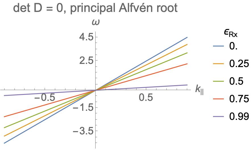
Figure 2: Showing transition of the Alfvén-branch dispersion relation: $\omega$ vs. $k_{\parallel}$; IMHD (${\varepsilon}_{\mathrm{Rx}}=0$) to RxMHD (${\varepsilon}_{\mathrm{Rx}}=1$: We have used ${\varepsilon}_{\mathrm{Rx}}=0.99$ for clarity as the ${\varepsilon}_{\mathrm{Rx}}=1$ line coincides with the $k_{\parallel}$ axis). Fixed parameters (in arb. units) are $k=1$, $\bm{u}=0$, $\bm{u}^{\rm Rx}=0$, $c_{{\rm s}}=1$ and $c_{{\rm A}}=5$. (Colour online. The vertical ordering of the lines in the $k_{\parallel}>0$ half plane coincides with that of ${\varepsilon}_{\mathrm{Rx}}$ in the legend.)

6.2.6 Dispersion relations — Alfvén branches

Multiplying the first factor of the determinant

$$\det\bm{\mathsf{D}}=\left(\omega_{\bm{k}}^{\prime\bm{u}}+{\varepsilon}_{\mathrm{Rx}}k_{\parallel}u^{{\rm Rx}}-{\varepsilon}_{\mathrm{I}}k_{\parallel}^{2}c_{{\rm A}}^{2}/\omega_{\bm{k}}^{\prime\bm{u}}\right)\det\bm{\mathsf{D}}_{{\rm MS}}$$ (130)

by $\omega_{\bm{k}}^{\prime\bm{u}}$ gives the dispersion relation for the Alfvén-wave branch(es) as the quadratic equation

$$\left(\omega_{\bm{k}}^{\prime\bm{u}}\right)^{2}+{\varepsilon}_{\mathrm{Rx}}k_{\parallel}u^{{\rm Rx}}\omega_{\bm{k}}^{\prime\bm{u}}-\left(1-{\varepsilon}_{\mathrm{Rx}}\right)k_{\parallel}^{2}c_{{\rm A}}^{2}=0\;.$$ (131)

The general solution of the quadratic equation is

$$\omega_{\bm{k}}^{\prime\bm{u}}=\frac{k_{\parallel}}{2}\left[-{\varepsilon}_{\mathrm{Rx}}u^{{\rm Rx}}\pm\left(4{\varepsilon}_{\mathrm{I}}c_{{\rm A}}^{2}+\left({\varepsilon}_{\mathrm{Rx}}u^{{\rm Rx}}\right)^{2}\right)^{1/2}\right]$$ (132)

Qualitative analysis is more informative: As ${\varepsilon}_{\mathrm{Rx}}\to 0$ the dispersion relations for the two branches approach the Doppler-shifted Alfvén-wave dispersion relations $\omega-\bm{k}\bm{\cdot}\bm{u}=\pm k_{\parallel}c_{{\rm A}}$. Also, inspection shows that $\omega-\bm{k}\bm{\cdot}\bm{u}\to 0$ as $k_{\parallel}\to 0$ quite generally, and when $\left|{\varepsilon}_{\mathrm{Rx}}\right|\ll 1$ the modification of the dispersion departure from the standard Alfvén-wave dispersion relation is essentially determined by the product ${\varepsilon}_{\mathrm{Rx}}u^{{\rm Rx}}$. Thus, when when $\left|{\varepsilon}_{\mathrm{Rx}}\right|\ll 1$ and the parallel flow parameter is at most Alfvénic, $u^{{\rm Rx}}/c_{{\rm A}}\leq O(1)$, ${\varepsilon}_{\mathrm{Rx}}$ and $u^{{\rm Rx}}$ will have little effect on the Alfvén-wave branches.

The plots in figure 2 give a visualization of the dependence of the dispersion relation on ${\varepsilon}_{\mathrm{Rx}}$. The figure is for a case where $\bm{u}^{\rm Rx}=0$, when (132) simplifies to $\omega_{\bm{k}}^{\prime\bm{u}}=\pm\sqrt{{\varepsilon}_{\mathrm{I}}}\,k_{\parallel}c_{{\rm A}}$. (We call the $+$ solution the principal branch.) The square root term $\sqrt{{\varepsilon}_{\mathrm{I}}}=\sqrt{1-{\varepsilon}_{\mathrm{Rx}}}$ gives rise to a singular dependence on ${\varepsilon}_{\mathrm{Rx}}$ at ${\varepsilon}_{\mathrm{Rx}}=1$ but the vicinity of IMHD is regular.

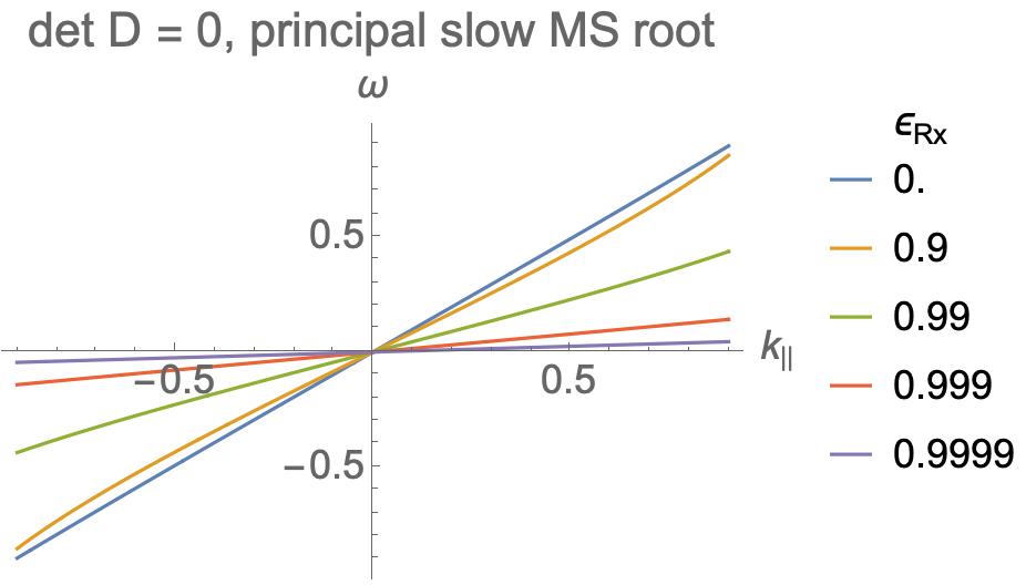
Figure 3: Showing transition of the slow-magnetosonic-branch dispersion relation: $\omega$ vs. $k_{\parallel}$; from IMHD (${\varepsilon}_{\mathrm{Rx}}=0$) to RxMHD (${\varepsilon}_{\mathrm{Rx}}=1$). Fixed parameters (in arb. units) are $k=1$, $\bm{u}=0$, $\bm{u}^{\rm Rx}=0$, $c_{{\rm s}}=1$ and $c_{{\rm A}}=5$. (Colour online. The vertical ordering of the lines in the $k_{\parallel}>0$ half plane coincides with that of ${\varepsilon}_{\mathrm{Rx}}$ in the legend.)

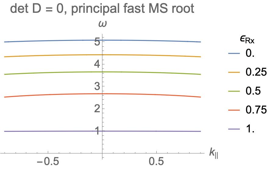
Figure 4: Showing transition of the fast-magnetosonic-branch dispersion relation: $\omega$ vs. $k_{\parallel}$; from IMHD (${\varepsilon}_{\mathrm{Rx}}=0$) to RxMHD (${\varepsilon}_{\mathrm{Rx}}=1$). Fixed parameters (in arb. units) are $k=1$, $\bm{u}=0$, $\bm{u}^{\rm Rx}=0$, $c_{{\rm s}}=1$ and $c_{{\rm A}}=5$. (Colour online. The vertical ordering of the lines in the $k_{\parallel}>0$ half plane coincides with that of ${\varepsilon}_{\mathrm{Rx}}$ in the legend.)

6.2.7 Dispersion relations — Magnetosonic branches

The magnetosonic dispersion relations are obtained by setting $\det\bm{\mathsf{D}}_{{\rm MS}}=0$, where

$$\det\bm{\mathsf{D}}_{{\rm MS}}=\frac{c_{{\rm A}}^{2}{\varepsilon}_{\mathrm{I}}k^{2}\left(k_{\parallel}^{2}c_{{\rm s}}^{2}-\omega^{2}\right)-\omega\left(c_{{\rm s}}^{2}k^{2}-\omega^{2}\right)({\varepsilon}_{\mathrm{Rx}}k_{\parallel}u^{{\rm Rx}}+\omega)}{\omega^{2}}\;.$$

The solution of the quartic equation $\omega^{2}\det\bm{\mathsf{D}}_{{\rm MS}}=0$ is extremely complicated but the figures 3 and 4 give an overview of the ${\varepsilon}_{\mathrm{Rx}}$ dependence. Again, the limit ${\varepsilon}_{\mathrm{Rx}}\to 1$ is clearly singular in the slow magnetosonic case but not ${\varepsilon}_{\mathrm{Rx}}\to 0$. This regularity around ideal MHD means our dispersion relation analysis is too crude to reveal the potential regularizing effect of softening the IOL constraint.

7 Conclusion

Invoking the augmented Lagrangian version of the penalty function method for constrained optimization, we have sketched out what we hope is a practical computational approach for iteratively solving the Relaxed MHD (RxMHD) Euler–Lagrange equations of Dewar et al. (2020)with added Ideal Ohm’s Law (IOL) constraint terms.

This method depends crucially on the existence of a Lagrange multiplier field to be found using the augmented Lagrangian iteration algorithm borrowed from finite-dimensional optimization theory.

A formal proof of convergence in may in general be difficult, but a practical approach will be to test the algorithm by perturbing away from IOL-feasible relaxed equilibria in simple geometries. A suitable such starting point is the rigidly rotating axisymmetric tokamak equilibrium discussed by Dewar et al. (2020). In this paper have illustrated the construction of the Lagrange multiplier field for linearized wave perturbations in the short-wavelength WKB approximation.

To find the constrained momentum equation we have used a little-known dyadic identity to derive a general conservation form. Substituting the constrained-RxMHD Lagrangian into this general form reveals residual terms in the stress tensor and a fictitious external force that should tend to zero uniformly in $\Omega$ if the constraint iteration converges so as to satisfy the IOL equality constraint.

However in non-axisymmetric, three-dimensional (3-D) plasma confinement systems such as stellarators and real tokamaks with field errors and intentionally resonant magnetic perturbations, there is good physical reason to believe uniform pointwise convergence is impossible. In such cases the best we can hope for is convergence in an $L^{2}$-norm, which will provide a weak-form regularization to cope with the singularities to which IMHD is prone in 3-D. This regularization should break the frozen-in flux condition of IMHD on small scales and allow interesting behaviour to be simulated without raising the order of the PDEs as adding resistivity does. Potential applications include reconnection events and the conjectured formation of equilibrium fractal magnetic and fluid flow patterns in 3-D systems. Other potential physical phenomena to investigate in 3-D systems include the linear normal mode spectrum, nonlinear saturation, bifurcations to oscillatory modes, and the effect of quasisymmetry [Nührenberg & Zille (1988); Burby et al. (2020); Rodriguez et al. (2020); Constantin et al. (2021)] on 3-D equilibria with flow [Vanneste & Wirosoetisno (2008)].

Also, to improve the physical applicability of relaxed MHD it will be important to extend the handling of thermal relaxation beyond isotropic pressure. Relaxation parallel to the magnetic field is very reasonable physically but perpendicular relaxation has forced the use of discontinuous pressure profiles in the MRxMHD-based SPEC code described by Hudson et al. (2012). Thus it will be important to build on the work of Dennis et al. (2014a) to include an anisotropic pressure tensor in a weakly IOL-feasible model.

N.B. An unabridged version of this paper with more detail on derivations of equations is available online as Supplementary Material at <link to be inserted by editors>.

Appendices

Appendix A A very brief history of relaxed MHD

The term relaxation in the physical sciences generally connotes a process by which a system tends toward an equilibrium state: thermodynamic, chemical, electrodynamic, mechanical, or a combination of these. For example, in a closed, constant energy system initially out of thermodynamic equilibrium, relaxation occurs as the entropy increases toward a maximum. In an open system at a temperature above that of a surrounding heat bath, relaxation occurs as heat carries energy out of the system, so its thermal energy tends toward a minimum.

In an open system with unbalanced mechanical forces, potential energy is converted into kinetic energy, which in turn is dissipated by friction into heat that is lost to the outside world, thus minimizing total energy, thermal and potential. This is the paradigm implicit in our use of the term “relaxation”, the assumption that a relaxed state is defined by the minimum of a Hamiltonian.

In plasma physics the first use of the term may have been in the paper by Chandrasekhar & Woltjer (1958), which proposes two variational principles other than maximizing entropy or minimizing energy: maximum energy for given mean-square current density and minimum dissipation for a given magnetic energy. The common element in these, and the minimum energy at constant magnetic helicity principle used by Woltjer (1958a) and Taylor Taylor (1974) is the derivation of a “linear-force-free” magnetic field obeying the Beltrami equation $\bm{\nabla}\bm{\times}\bm{B}=\mu\bm{B}$, with $\mu$ constant, as the outcome. The Chandrasekhar and Woltjer work was in the context of plasma astrophysics, justifying the force-free assumption (where the force density in question is $\bm{j}\bm{\times}\bm{B}$) basically on the assumption the plasma has low $\beta\stackrel{{\scriptstyle\text{def}}}{{=}}p/\left(B^{2}/2\upmu_{0}\right)$ and no confining forces that are strong compared with gradients of magnetic pressure. In contrast Taylor considered a toroidal terrestrial plasma confined in a metal shell and driven by a strong induced current, creating a turbulent state from which the plasma relaxes. Taylor regards the relaxation mechanism as the breaking of the microscopic IMHD topological invariants leaving only the global magnetic helicity as conserved.

Taylor (1974) is uncommital as to the exact details of this breaking of microscopic invariants and is content to use successful comparison with experiment of the predictions flowing from his derivation of the Beltrami equation as sufficient validation of his elegantly simple model, a general philosophy we also adopt. However in his later review, Taylor (1986) gives some more detail on the decay mechanism, citing some turbulence simulations and invokes turbulence scale length arguments to explain why it is energy that is minimized rather than magnetic helicity. Moffatt (2015) has recently critically reviewed the arguments of Taylor (1986) from a more modern perspective.

Woltjer (1958b) pointed out there were other global IMHD invariants beyond magnetic helicity, in particular his eq. (2), the cross helicity involving both flow and magnetic field. Bhattacharjee & Dewar (1982) pointed that in an axisymmetric system an infinity of additional global invariants could be generated by taking moments of $\bm{A}\bm{\cdot}\bm{B}$ with powers of a flux function, and used lower moments to generate more physical pressure and current profiles for tokamak equilibria than the very restricted profiles given by Taylor’s relaxation principle. Hudson et al. (2012) developed multi-region relaxed MHD (MRxMHD), a generalization of single-region Taylor relaxation by inserting thin IMHD barrier interface tori to frustrate global Taylor relaxation. This generalization is appropriate to non-axisymmetric equilibria in stellarators and in tokamaks with symmetry-breaking perturbations, where magnetic field-line flow can be chaotic even without turbulence. This MRxMHD formulation is implemented in the now well-established Stepped-Pressure Equilibrium Code (SPEC).

A relaxation approach for finding equilibria with flow by adding a constraint additional to conservation of magnetic helicity, conservation of cross helicity, was used by Finn and Antonsen Finn & Antonsen (1983) using an entropy-maximization relaxation principle [see also the contemporaneous paper by Hameiri Hameiri (1983)]. However, they show this leads to the same equations as energy minimization. Thus we take, as in IMHD, the entropy in $\Omega$ to be conserved and follow Taylor in defining relaxed states as energy minima.

Pseudo-dynamical energy-descent relaxation processes that conserve topological invariants have been developed, Vallis et al. (1989); Vladimirov et al. (1999) but we stay within the framework of conservative classical mechanics by developing a dynamical formalism, RxMHD, that includes relaxed equilibria as stationary points of a relaxation Hamiltonian, with Lagrange multipliers to constrain chosen macroscopic invariants, but which also allows non-equilibrium motions, most easily done using Hamilton’s action principle. Stability can also be examined by taking the second variation of the Hamiltonian, Vladimirov et al. (1999) but in this paper, as in Dewar et al. (2015) and Dewar et al. (2020)we deal only with first variations.

However the SPEC code implements a Newton method for finding energy minima and saddle points by calculating a Hessian matrix, which is the second variation of the MRxMHD energy. Combined with a model kinetic energy obtained by loading all mass onto the interfaces between the relaxation regions. This has recently been used successfully by Kumar et al. (2021, Submitted 2021) for calculating the spectrum of some linear eigenmodes in a tokamak, but comparison between the model kinetic energy and our new dynamical relaxation theory is desirable for determining the domain of applicability of the mass loading model.

Appendix B Some vector and dyadic identities

In the body of this paper we have used the usual coordinate-free vector (and dyadic) calculus notations, but in this appendix we derive some identities that are more easily proved using elementary tensor notation. Assuming an arbitrary fixed orthonormal basis $\{\bm{e}_{i}\}$, $i=1,2,3\mod 3$, a vector, $\bm{a}$ say, is represented as $\bm{a}=a_{i}\bm{e}_{i}$, the summation convention for contraction over repeated dummy indices being assumed throughout.

Thus dot and cross products are represented as $\bm{a}\cdot\bm{b}=a_{i}b_{i}$ and $\bm{a}\bm{\times}\bm{b}=\bm{e}_{i}\varepsilon_{i,j,k}a_{j}b_{k}$, respectively, where the alternating Levi-Civita tensor $\varepsilon_{ijk}$ is $1$ or $-1$ according as $\{i,j,k\}$ is an even or odd permutation of $\{1,2,3\}$, or $0$ if it is neither (e.g. if there are repeated integers). Also the operations of grad and curl acting on scalar and vector functions $f$ and $\bm{f}$, respectively, are represented as $\bm{\nabla}f=\partial f/\partial\bm{x}\stackrel{{\scriptstyle\text{def}}}{{=}}\bm{e}_{i}\partial_{i}f$ and $\bm{\nabla}\bm{\times}\bm{a}\stackrel{{\scriptstyle\text{def}}}{{=}}\bm{e}_{i}\varepsilon_{ijk}\partial_{j}a_{k}$, where $\partial_{i}\stackrel{{\scriptstyle\text{def}}}{{=}}\partial/\partial x_{i}$. We use parentheses to limit the scope of the rightward differentiation of such operators. NB Left-right ordering is more important in vector notation. E.g. the dyadics $\bm{a}\bm{b}$ and $\bm{b}\bm{a}$ are distinct, but $a_{i}b_{j}=b_{j}a_{i}$.

First we derive three useful identities involving gradients with respect to $\bm{B}\equiv B_{i}\bm{e}_{i}$, and the unit vector parallel to $\bm{B}$, $\bm{e}_{\bm{B}}(\bm{x})\equiv\bm{B}(\bm{x})/B(\bm{x})$. (By “parallel to $\bm{B}$” we mean locally tangent to the magnetic field line passing though any point $\bm{x}$. Henceforth the dependence on $\bm{x}$ is implicit as these identities concern functions purely of $\bm{B}$.):

Lemma 1.

The gradients of $\bm{B}$, $B$ and $\bm{e}_{B}$ with respect to $\bm{B}$ are, in terms of the identity dyadic $\bm{\mathsf{I}}\stackrel{{\scriptstyle\text{def}}}{{=}}\sum_{i}\bm{e}_{i}\bm{e}_{i}$, the unit tangent vector $\bm{e}_{\bm{B}}$, and $\bm{\mathsf{P}}_{\perp}\stackrel{{\scriptstyle\text{def}}}{{=}}\bm{\mathsf{I}}-\bm{e}_{\bm{B}}\bm{e}_{\bm{B}}$, the projector onto the plane perpendicular to $\bm{B}$,

$$\frac{\partial\bm{B}}{\partial\bm{B}}=\bm{\mathsf{I}},\quad\frac{\partial B}{\partial\bm{B}}=\bm{e}_{\bm{B}},\;\;\text{and}\quad\frac{\partial\bm{e}_{\bm{B}}}{\partial\bm{B}}=\frac{\bm{\mathsf{P}}_{\perp}}{B}\;.$$ (133)

Derivations: Using the notations $\partial_{\bm{B}}\cdot\equiv\bm{e}_{i}\partial_{B_{i}}\equiv\partial\cdot/\partial\bm{B}$, we have the obvious identity $\partial_{\bm{B}}\bm{B}=\bm{\mathsf{I}}$. Applying this first identity to $B\equiv(\bm{B}\bm{\cdot}\bm{B})^{1/2}$ we find the second identity, $\partial_{\bm{B}}B=\left(2\bm{\mathsf{I}}\bm{\cdot}\bm{B}\right)/2B=\bm{B}/B=\bm{e}_{\bm{B}}$. The third identity follows from the first two: $\partial_{\bm{B}}\left(\bm{B}/B\right)=\bm{\mathsf{I}}/B-\bm{B}$$\bm{e}_{\bm{B}}$$/B^{2}=\left(\bm{\mathsf{I}}-\bm{e}_{\bm{B}}\bm{e}_{\bm{B}}\right)/B$. $\quad\Box$

Lemma 2.

Variational derivative of functional $F[\bm{A},\Phi]=\iint\!\!f(\bm{A},\bm{B},\bm{E})\mathrm{d}V\mathrm{d}t$ is

$$\frac{\delta F}{\delta\bm{A}}=\frac{\partial f}{\partial\bm{A}}+\bm{\nabla}\bm{\times}\frac{\partial f}{\partial\bm{B}}+\frac{\partial}{\partial t}\frac{\partial f}{\partial\bm{E}}\;,$$ (134)

where $f$ is an arbitrary scalar-valued function of $\bm{A}$, $\bm{B}=\bm{\nabla}\bm{\times}{\bm{A}}$, and $\bm{E}=-\partial_{t}$$\bm{A}-\bm{\nabla}\Phi$ from (6), $\bm{A}$ being an arbitrary vector field.

Varying $\bm{A}$

$$\delta F =\iint\left[\frac{\partial f}{\partial\bm{A}}\bm{\cdot}\delta\bm{A}+\frac{\partial f}{\partial\bm{B}}\bm{\cdot}\bm{\nabla}\bm{\times}\delta\bm{A}-\frac{\partial f}{\partial\bm{E}}\bm{\cdot}\partial_{t}\delta\bm{A}\right]\mathrm{d}V\mathrm{d}t$$

$$=\iint\left[\frac{\partial f}{\partial A_{i}}\delta A_{i}+\frac{\partial f}{\partial B_{i}}\varepsilon_{i,j,k}\partial_{j}\delta A_{k}-\frac{\partial f}{\partial E_{i}}\partial_{t}\delta A_{i}\right]\mathrm{d}V\mathrm{d}t$$

$$=\iint\left[\frac{\partial f}{\partial A_{i}}\delta A_{i}-\varepsilon_{k,j,i}\left(\partial_{j}\frac{\partial f}{\partial B_{k}}\right)\delta A_{i}+\left(\partial_{t}\frac{\partial f}{\partial E_{i}}\right)\delta A_{i}\right]\mathrm{d}V\mathrm{d}t\;,\quad i\rightleftarrows k\>\&\>\text{ibp}$$

$$=\iint\left[\frac{\partial f}{\partial A_{i}}+\varepsilon_{i,j,k}\left(\partial_{j}\frac{\partial f}{\partial B_{k}}\right)+\left(\partial_{t}\frac{\partial f}{\partial E_{i}}\right)\right]\delta A_{i}\,\mathrm{d}V\mathrm{d}t\;,\quad\varepsilon_{k,j,i}=-\varepsilon_{i,j,k}$$

$$=\iint\left(\frac{\partial f}{\partial\bm{A}}+\bm{\nabla}\bm{\times}\frac{\partial f}{\partial\bm{B}}+\frac{\partial}{\partial t}\frac{\partial f}{\partial\bm{E}}\right)\!\bm{\cdot}\!\delta\bm{A}\,\mathrm{d}V\mathrm{d}t\stackrel{{\scriptstyle\text{def}}}{{=}}\int\!\frac{\delta F}{\delta\bm{A}}\bm{\cdot}\delta\bm{A}\,\mathrm{d}V\mathrm{d}t\;,$$

where $\rightleftarrows$ stands for “have swapped dummy indices” and “ibp” stands for “have integrated by parts” (neglecting surface terms on the assumption that the supports of variations do not include the boundary).$\quad\Box$

Lemma 3.

Variational derivative of functional $F$ above is

$$\frac{\delta F}{\delta\Phi}=\bm{\nabla\cdot}\frac{\partial f}{\partial\bm{E}}\;,$$ (135)

Derivation: Varying $\Phi$

$$\delta F =\iint\left[-\frac{\partial f}{\partial\bm{E}}\bm{\cdot}\bm{\nabla}\delta\Phi\right]\mathrm{d}V\mathrm{d}t$$

$$=\iint\left[\left(\bm{\nabla\cdot}\frac{\partial f}{\partial\bm{E}}\right)\delta\Phi\right]\mathrm{d}V\mathrm{d}t\stackrel{{\scriptstyle\text{def}}}{{=}}\int\!\frac{\delta F}{\delta\Phi}\delta\Phi\,\mathrm{d}V\mathrm{d}t\;,$$

neglecting surface term as above.$\quad\Box$

Two useful identities, closely related to integration by parts, for deriving conservation forms of Euler–Lagrange equations for freely variable fields [members of the set denoted $\bm{\upeta}$ in Dewar et al. (2020)] are

Lemma 4.

For scalar fields, e.g. $\Phi$

$$(\bm{\nabla}\bm{\nabla}\Phi)\bm{\cdot}\bm{f}=\bm{\nabla\cdot}[\bm{f}\bm{\nabla}\Phi]-(\bm{\nabla}\Phi)\bm{\nabla\cdot}\bm{f}\;,$$ (136)

where $\bm{f}$ is an arbitrary vector field, e.g. $\partial\mathcal{L}/\partial\bm{\nabla}\Phi$.

Derivation: Follows directly from fact $\bm{\nabla}\bm{\nabla}\Phi$ is a symmetric dyadic, proved in first line below,

$$(\bm{\nabla}\bm{\nabla}\Phi)\bm{\cdot}\bm{f} =\bm{e}_{i}(\partial_{i}\partial_{j}\Phi)f_{j}=\bm{e}_{i}(\partial_{j}\partial_{i}\Phi)f_{j}\;,\quad\partial_{i}\rightleftharpoons\partial_{j}$$

$$=\bm{e}_{i}(\partial_{j}\partial_{i}\Phi f_{j})-\bm{e}_{i}(\partial_{i}\Phi)\partial_{j}f_{j}$$

$$=\bm{\nabla\cdot}[\bm{f}\bm{\nabla}\Phi]-(\bm{\nabla}\Phi)\bm{\nabla\cdot}\bm{f}\;,$$

where $\rightleftharpoons$ stands for “have commuted operators”.$\Box$

Corollary 1.

For $\bm{E}=-\bm{\nabla}\Phi-\partial_{t}\bm{A}$,

$$\left(\bm{\nabla}\bm{E}\right)\bm{\cdot}\bm{f}=\bm{\nabla\cdot}[\bm{f}\bm{E}]-\bm{E}\bm{\nabla\cdot}\bm{f}-\bm{f}\bm{\times}\partial_{t}\bm{B}\;.$$ (137)

Derivation: Muliplying each side of (136) by $-1$, writing $-\bm{\nabla}\Phi=\bm{E}+\partial_{t}\bm{A}$ and subtracting $\partial_{t}\bm{A}$ from both sides, the lemma (136) becomes

$$\left(\bm{\nabla}\bm{E}\right)\bm{\cdot}\bm{f} =\bm{\nabla\cdot}[\bm{f}\bm{(E}+\partial_{t}\bm{A})]-\bm{(E}+\partial_{t}\bm{A})\bm{\nabla\cdot}\bm{f}-(\bm{\nabla}\partial_{t}\bm{A})\bm{\cdot}\bm{f}\;,$$

$$=\bm{\nabla\cdot}[\bm{f}\bm{E}]-\bm{E}\bm{\nabla\cdot}\bm{f}+\bm{\nabla\cdot}[\bm{f}\partial_{t}\bm{A}]-\left(\partial_{t}\bm{A}\right)\bm{\nabla\cdot}\bm{f}-(\bm{\nabla}\partial_{t}\bm{A})\bm{\cdot}\bm{f}$$

$$=\bm{\nabla\cdot}[\bm{f}\bm{E}]-\bm{E}\bm{\nabla\cdot}\bm{f}+\bm{f}\bm{\cdot}(\bm{\nabla}\partial_{t}\bm{A})-(\bm{\nabla}\partial_{t}\bm{A})\bm{\cdot}\bm{f}$$

$$=\bm{\nabla\cdot}[\bm{f}\bm{E}]-\bm{E}\bm{\nabla\cdot}\bm{f}-\bm{f}\bm{\times}(\bm{\nabla}\bm{\times}\partial_{t}\bm{A})$$

$$=\bm{\nabla\cdot}[\bm{f}\bm{E}]-\bm{E}\bm{\nabla\cdot}\bm{f}-\bm{f}\bm{\times}\partial_{t}\bm{B}\;.\Box$$

Lemma 5.

For $\bm{A}$ an arbitrary vector field and $\bm{B}=\bm{\nabla}\bm{\times}\bm{A},$

$$(\bm{\nabla}\bm{B})\bm{\cdot}\bm{f}=-\bm{\nabla\cdot}[\bm{f}\bm{\times}(\bm{\nabla}\bm{A})^{{\rm T}}]+(\bm{\nabla}\bm{A})\bm{\cdot}\bm{\nabla}\bm{\times}\bm{f}\;,$$ (138)

where $\bm{f}$ is an arbitrary vector field, e.g. $\partial\mathcal{L}/\partial\bm{B}$. [N.B. For a more useful form see the corollary (139) below.]

Derivation:

$$(\bm{\nabla}\bm{\nabla}\bm{\times}\bm{A})\bm{\cdot}\bm{f} =\bm{e}_{i}(\partial_{i}\varepsilon_{j,k,l}\partial_{k}A_{l})f_{j}=\bm{e}_{i}(\partial_{k}\varepsilon_{j,k,l}\partial_{i}A_{l})f_{j}\;,\quad\partial_{i}\rightleftharpoons\partial_{k}$$

$$=\bm{e}_{i}\partial_{k}[(\partial_{i}A_{l})\varepsilon_{j,k,l}f_{j}]-\bm{e}_{i}(\partial_{i}A_{l})\varepsilon_{j,k,l}\partial_{k}f_{j}$$

$$=-\partial_{k}[\varepsilon_{k,j,l}f_{j}(\bm{\nabla}A_{l})]+(\bm{\nabla}A_{l})\varepsilon_{l,k,j}\partial_{k}f_{j}\;,\quad\text{anticyclic perms. of }j,k,l$$

$$=-\bm{\nabla\cdot}[\bm{f}\bm{\times}(\bm{\nabla}\bm{A})^{{\rm T}}]+(\bm{\nabla}\bm{A})\bm{\cdot}\bm{\nabla}\bm{\times}\bm{f}\;,$$

where $(\bm{\nabla}\bm{A})^{{\rm T}}$ is the transpose of the dyadic $\bm{\nabla}\bm{A}$.$\quad\Box$

Corollary 2.

$$(\bm{\nabla}\bm{B})\bm{\cdot}\bm{f} =\left(\bm{\nabla}\bm{\times}\bm{f}\right)\bm{\times}\bm{B}-\bm{\nabla\cdot}\left[\bm{f}\bm{\times}\bm{\mathsf{I}}\bm{\times}\bm{B}\right]$$ (139)

Derivation: Because of the identity $\bm{\nabla\cdot}\left(\bm{f}\bm{\times}\bm{\nabla}\bm{A}\right)-\left(\bm{\nabla}\bm{\times}\bm{f}\right)\bm{\cdot}\bm{\nabla}\bm{A}=0$ (which is easily proven using the properties of the scalar product and the identity $\bm{\nabla}\bm{\times}\bm{\nabla}=0$) we can add $\bm{\nabla\cdot}\left(\bm{f}\bm{\times}\bm{\nabla}\bm{A}\right)-(\bm{\nabla}\bm{A})^{{\rm T}}\bm{\cdot}\left(\bm{\nabla}\bm{\times}\bm{f}\right)$ to the RHS of (138) to antisymmetrize $\bm{\nabla}\bm{A}$ and thus to eliminate it in favour of $\bm{\nabla}\bm{\times}\bm{A}=\bm{B}$:

$$(\bm{\nabla}\bm{B})\bm{\cdot}\bm{f} =\bm{\nabla\cdot}\left[\bm{f}\bm{\times}\left(\bm{\nabla}\bm{A}-(\bm{\nabla}\bm{A})^{{\rm T}}\right)\right]+\left(\bm{\nabla}\bm{A}-(\bm{\nabla}\bm{A})^{{\rm T}}\right)\bm{\cdot}\bm{\nabla}\bm{\times}\bm{f}$$

$$=-\bm{\nabla\cdot}\left[\bm{f}\bm{\times}\bm{\mathsf{I}}\bm{\times}\left(\bm{\nabla}\bm{\times}\bm{A}\right)\right]+\left(\bm{\nabla}\bm{\times}\bm{f}\right)\bm{\times}\left(\bm{\nabla}\bm{\times}\bm{A}\right)$$

the second term in the second line following from

$$\bm{f}\bm{\times}\left(\bm{\nabla}\bm{A}-(\bm{\nabla}\bm{A})^{{\rm T}}\right) =\bm{f}\bm{\times}\bm{e}_{i}\bm{e}_{i}\bm{\cdot}\left(\bm{\nabla}\bm{A}-(\bm{\nabla}\bm{A})^{{\rm T}}\right)$$

$$=-\bm{f}\bm{\times}\bm{e}_{i}\bm{e}_{i}\bm{\times}\left(\bm{\nabla}\bm{\times}\bm{A}\right)\quad\Box$$

Alternatively, verify without using vector potential but assuming $\bm{\nabla\cdot}\bm{B}=0$:

RHS $$=\left(\bm{\nabla}\bm{\times}\bm{f}\right)\bm{\times}\bm{B}-\bm{\nabla\cdot}\left[\bm{f}\bm{\times}\bm{e}_{i}\bm{e}_{i}\bm{\times}\bm{B}\right]$$

$$=\>\left(\bm{\nabla}\bm{\times}\bm{f}\right)\bm{\times}\bm{B}-\left(\bm{\nabla}\bm{\times}\bm{f}\right)\bm{\cdot}\bm{e}_{i}\bm{e}_{i}\bm{\times}\bm{B}$$

$$\qquad+\bm{f}\bm{\cdot}\bm{e}_{j}\bm{\times}\bm{\nabla}\bm{B}\bm{\times}\bm{e}_{j}$$

$$=-\bm{e}_{m}f\varepsilon_{j,i,k}\varepsilon_{j,m,l}\partial_{k}B_{l}$$

$$=-\bm{e}_{m}f_{i}\left(\delta_{i,m}\delta_{k,l}-\delta_{i,l}\delta_{k,m}\right)\partial_{k}B_{l}$$

$$=\bm{e}_{k}f_{i}\partial_{k}B_{i}-\bm{e}_{i}f_{i}\partial_{k}B_{k}$$

$$=\left(\bm{\nabla}\bm{B}\right)\bm{\cdot}\bm{f}-\bm{f}\bm{\nabla\cdot}\bm{B}$$

$$=\text{LHS}\quad\Box\;,$$

where we used the Levi-Civita tensor contraction result $\varepsilon_{a,b,c}\varepsilon_{a,j,k}=\delta_{b,j}\delta_{c,k}-\delta_{b,k}\delta_{c,j}$, where here $\delta$ is the Kronecker symbol.

Lemma 6.

$$\bm{f}\bm{\times}\bm{\mathsf{I}}\bm{\times}\bm{g}=\bm{g}\bm{f}-\bm{{f}}\!\bm{\cdot}\!\bm{{g}}\,\bm{\mathsf{I}}$$ (140)

Derivation:

$$\left(\bm{f}\bm{\times}\bm{\mathsf{I}}\bm{\times}\bm{g}\right)_{i,j} =f_{k}\bm{e}_{i}\bm{\cdot}\bm{e}_{k}\bm{\times}\bm{e}_{l}\bm{e}_{l}\bm{\times}\bm{e}_{m}\bm{\cdot}\bm{e}_{j}g_{m}$$

$$=f_{k}\varepsilon_{i,k,l}\varepsilon_{l,m,j}g_{m}=f_{k}\varepsilon_{l,i,k}\varepsilon_{l,m,j}g_{m}$$

$$=f_{k}\left(\delta_{i,m}\delta_{k,j}-\delta_{i,j}\delta_{k,m}\right)g_{m}$$

$$=f_{j}g_{i}-f_{k}g_{k}\delta_{i,j}\>\>\Box$$

Verification:

$$\bm{a}\bm{\cdot}\text{\text{LHS}} =\bm{a}\bm{\cdot}\bm{f}\bm{\times}\bm{\mathsf{I}}\bm{\times}\bm{g}$$

$$=\bm{a}\bm{\times}\bm{f}\bm{\cdot}\bm{\mathsf{I}}\bm{\times}\bm{g}$$

$$=\left(\bm{a}\bm{\times}\bm{f}\right)\bm{\times}\bm{g}$$

$$=\left(\bm{a}\bm{\cdot}\bm{g}\right)\bm{f}-\left(\bm{f}\bm{\cdot}\bm{g}\right)\bm{a}$$

$$=\bm{a}\bm{\cdot}\text{\text{RHS}$\quad$}\forall\>\bm{a}\>.\>\Box$$

$$\text{LHS}\bm{\cdot}\text{$\bm{b}$} =\bm{f}\bm{\times}\bm{\mathsf{I}}\bm{\cdot}\left(\bm{g}\bm{\times}\bm{b}\right)$$

$$=\bm{f}\bm{\times}\left(\bm{g}\bm{\times}\bm{b}\right)$$

$$=\left(\bm{f}\bm{\cdot}\bm{b}\right)\bm{g}-\left(\bm{f}\bm{\cdot}\bm{g}\right)\bm{b}$$

$$=\text{RHS}\bm{\cdot}\text{\text{$\bm{b}$}$\quad$}\forall\>\bm{b}\>.\>\Box$$

References

- Bhattacharjee & Dewar (1982) Bhattacharjee, A. & Dewar, R. L. 1982 Energy principle with global invariants. Phys. Fluids 25, 887–897.
- Burby (2017) Burby, J. W. 2017 Magnetohydrodynamic motion of a two-fluid plasma. Phys. Plasmas 24, 082104–1–13.
- Burby et al. (2020) Burby, J. W., Kallinikos, N. & MacKay, R. S. 2020 Some mathematics for quasi-symmetry. J. Math. Phys. 61, 093503–1–22.
- Calkin (1963) Calkin, M. G. 1963 An action principle for magnetohydrodynamics. Can. J. Phys. 41, 2241–2251.
- Chandrasekhar & Woltjer (1958) Chandrasekhar, S. & Woltjer, L. 1958 On force-free magnetic fields. Proc. Nat. Acad. Sci. (U.S.) 44, 285.
- Constantin et al. (2021) Constantin, P., Drivas, T. D. & Ginsberg, D. 2021 On quasisymmetric plasma equilibria sustained by small force. J. Plasma Phys. 87, 905870111–1–30.
- Dennis et al. (2014a) Dennis, G. R., Hudson, S. R., Dewar, R. L. & Hole, M. J. 2014a Multi-region relaxed magnetohydrodynamics with anisotropy and flow. Phys. Plasmas 21, 072512–1–10.
- Dennis et al. (2014b) Dennis, G. R., Hudson, S. R., Dewar, R. L. & Hole, M. J. 2014b Multi-region relaxed magnetohydrodynamics with flow. Phys. Plasmas 21, 042501–1–9.
- Dewar (1970) Dewar, R. L. 1970 Interaction between hydromagnetic waves and a time-dependent, inhomogeneous medium. Phys. Fluids 13, 2710–2720.
- Dewar (1977) Dewar, R. L. 1977 Energy-momentum tensors for dispersive electromagnetic waves. Australian J. Phys. 30, 533.
- Dewar et al. (2020) Dewar, R. L., Burby, J. W., Qu, Z. S., Sato, N. & Hole, M. J. 2020 Time-dependent relaxed magnetohydrodynamics – inclusion of cross helicity constraint using phase-space action. Phys. Plasmas 27, 062504–1–22.
- Dewar et al. (2015) Dewar, R. L., Yoshida, Z., Bhattacharjee, A. & Hudson, S. R. 2015 Variational formulation of relaxed and multi-region relaxed magnetohydrodynamics. J. Plasma Phys. 81, 515810604.
- Fathi (2009) Fathi, A. 2009 Weak KAM Theorem in Lagrangian Dynamics. Cambridge Studies in Advanced Mathematics 88. Cambridge, U.K.: Cambridge University Press.
- Finn & Antonsen (1983) Finn, J. M. & Antonsen, Jr., T. M. 1983 Turbulent relaxation of compressible plasmas with flow. Physics of Fluids 26, 3540.
- Frieman & Rotenberg (1960) Frieman, E. & Rotenberg, M. 1960 On hydromagnetic stability of stationary equilibria. Rev. Mod. Phys. 32, 898–902.
- Goldstein (1980) Goldstein, H. 1980 Classical Mechanics, 2nd edn. Reading, Mass., USA: Addison-Wesley.
- Grad (1967) Grad, H. 1967 Toroidal containment of a plasma. Phys. Fluids 10, 137–154.
- Hameiri (1983) Hameiri, E. 1983 The equilibrium and stability of rotating plasmas. Phys. Fluids 26, 230–237.
- Hameiri (1998) Hameiri, E. 1998 Variational principles for equilibrium states with plasma flow. Phys. Plasmas 5, 3270–3281.
- Hameiri (2014) Hameiri, E. 2014 Some improvements in the theory of plasma relaxation. Phys. Plasmas 21, 044503–1–5.
- Hosking & Dewar (2015) Hosking, R. J. & Dewar, R. L. 2015 Fundamental Fluid Mechanics and Magnetohydrodynamics. Singapore: Springer Singapore, published online 2015. Book copyright 2016.
- Hudson et al. (2012) Hudson, S. R., Dewar, R. L., Dennis, G., Hole, M. J., McGann, M., von Nessi, G. & Lazerson, S. 2012 Computation of multi-region relaxed magnetohydrodynamic equilibria. Phys. Plasmas 19, 112502–1–18.
- Kanzow et al. (2018) Kanzow, C., Steck, D. & Wachsmuth, D. 2018 An augmented Lagrangian method for optimization problems in Banach spaces. SIAM J. Control Optim. 56, 272–291.
- Kumar et al. (Submitted 2021) Kumar, A., Qu, Z., Doak, J., Dewar, R. L., Hezaveh, H., Nührenberg, C., Aleynikova, K., Hole, M. J., Hudson, S. R., Loizu, J. & Baillod, A. Submitted 2021 Ideal MHD instabilities of Multi-Region relaxed MHD. Plasma Phys. Control Fusion .
- Kumar et al. (2021) Kumar, A., Qu, Z., Hole, M. J., Wright, A. M., Loizu, J., Hudson, S. R., Baillod, A., Dewar, R. L. & Ferraro, N. M. 2021 Computation of linear MHD instabilities with the multi-region relaxed MHD energy principle. Plasma Phys. Control. Fusion 63, 045006.
- Levnajić & Mezić (2010) Levnajić, Z. & Mezić, I. 2010 Ergodic theory and visualization. i. mesochronic plots for visualization of ergodic partition and invariant sets. Chaos 20, 033114.
- Meiss (1992) Meiss, J. D. 1992 Symplectic maps, variational principles, and transport. Rev. Mod. Phys. 64, 795–848.
- Mezić & Wiggins (1999) Mezić, I. & Wiggins, S. 1999 A method for visualization of invariant sets of dynamical systems based on the ergodic partition. Chaos 9, 213.
- Moffatt (2015) Moffatt, H. K. 2015 Magnetic relaxation and the Taylor conjecture. J. Plasma Phys. 81, 905810608.
- Morrison (1998) Morrison, P. J. 1998 Hamiltonian description of the ideal fluid. Rev. Mod. Phys. 70, 467–521.
- Newcomb (1958) Newcomb, W. A. 1958 Motion of magnetic lines of force. Ann. Phys. 3 (4), 347–385.
- Newcomb (1962) Newcomb, W. A. 1962 Lagrangian and Hamiltonian methods in magnetohydrodynamics. Nucl. Fusion Suppl. Part 2, 451–463.
- Nocedal & Wright (2006) Nocedal, J. & Wright, S. J. 2006 Numerical Optimization, 2nd edn. Operation Research and Financial Engineering 25. New York: Springer.
- Nührenberg & Zille (1988) Nührenberg, J. & Zille, R. 1988 Quasi-helically symmetric toroidal stellarators. Phys. Lett. A 129, 113–117.
- Panofsky & Phillips (1962) Panofsky, W. K. H. & Phillips, M. 1962 Classical Electricity and Magnetism, 2nd edn. Reading, Mass., USA: Addison-Wesley.
- Qu et al. (2020) Qu, Z. S., Dewar, R. L., Ebrahimi, F., Anderson, J. K., Hudson, S. R. & Hole, M. J. 2020 Stepped pressure equilibrium with relaxed flow and applications in reversed-field pinch plasmas. Plasma Phys. Control. Fusion 62, 054002, preprint arXiv:2001.06984.
- Qu et al. (2021) Qu, Z. S., Hudson, S. R., Dewar, R. L., Loizu, J. & Hole, M. J. 2021 On the non-existence of stepped-pressure equilibria far from symmetry. Plasma Phys. Control Fusion 63, 125007.
- Rodriguez et al. (2020) Rodriguez, E., Helander, P. & Bhattacharjee, A. 2020 Necessary and sufficient conditions for quasisymmetry. Phys. Plasmas 27, 062501–1–5.
- Taylor (1974) Taylor, J. B. 1974 Relaxation of toroidal plasma and generation of reverse magnetic fields. Phys. Rev. Lett. 33, 1139–1141.
- Taylor (1986) Taylor, J. B. 1986 Relaxation and magnetic reconnection in plasmas. Rev. Mod. Phys. 58, 741–763.
- Vallis et al. (1989) Vallis, G. K., Carnevale, G. F. & Young, W. R. 1989 Extremal energy properties and construction of stable solutions of the Euler equations. J. Fluid Mech. 207 (133–152).
- Vanneste & Wirosoetisno (2008) Vanneste, J. & Wirosoetisno, D. 2008 Two-dimensional Euler flows in slowly deforming domains. Physica D, 774-799 237, 774–799.
- Vladimirov et al. (1999) Vladimirov, V. A., Moffatt, H. K. & Ilin, K. I. 1999 On general transformations and variational principles for the magnetohydrodynamics of ideal fluids. part 4. generalized isovorticity principle for three-dimensional flows. J. Fluid Mech. 390, 127–150.
- Webb (2018) Webb, G. M. 2018 Magnetohydrodynamics and Fluid Dynamics: Action Principles and Conservation Laws, Lecture Notes in Physics, vol. 946. Springer International Publishing.
- Webb & Anco (2017) Webb, G. M. & Anco, S. C. 2017 On magnetohydrodynamic gauge field theory. J. Phys. A: Math. Theor. 50, 255501–1–34.
- Webb & Anco (2019) Webb, G. M. & Anco, S. C. 2019 Conservation laws in magnetohydrodynamics and fluid dynamics: Lagrangian approach. AIP Conf. Proc. 2153, 020024.
- Woltjer (1958a) Woltjer, L. 1958a A theorem on force-free magnetic fields. Proc. Nat. Acad. Sci. (U.S.) 44, 489–491.
- Woltjer (1958b) Woltjer, L. 1958b On hydromagnetic equilibrium. Proc. Nat. Acad. Sci. (U.S.) 44, 833.
- Yokoi (2013) Yokoi, N. 2013 Cross helicity and related dynamo. Geophys. Astrophys. Fluid Dyn. 107, 114–184.