Packing theory derived from phyllotaxis and products of linear forms.

Abstract

Parastichies are spiral patterns observed in plants and numerical patterns generated using golden angle method. We generalize this method by using Markoff theory and the theory of product of linear forms, to obtain a theory for packing of Riemannian manifolds of general dimensions $n$ with a locally diagonalizable metric, including the Euclidean spaces. For example, packings in a plane with logarithmic spirals and in a ball are newly obtained. Using this method, we prove that it is possible to generate almost uniformly distributed point sets on any real analytic Riemannian surfaces. The packing density is bounded below by approximately 0.7.

Keywords: aperiodic packing; Markoff spectra; Lagrange spectra; products of linear forms; diagonalizable metric; inviscid Burgers equation; Vogel spiral; Doyle spiral

1 Introduction

In botany, spiral patterns observed in plants, such as sunflower heads, cacti, and pinecones, are called parastichies. Parastichies can also be observed in patterns that are numerically generated on a surface with circular symmetry using golden angle method. In the golden angle method, a new point is generated for each $2\pi\varphi\approx 137.5^{\circ}$-rotation, where $\varphi=1/(1+\gamma_{1})$ is the golden angle defined using the golden ratio $\gamma_{1}=(1+\sqrt{5})/2$. With this method, packng patterns have been generated on a cylindrical surface [8], a disk known as the Vogel spiral [25], [38] (Figure 1), surfaces of revolution [30], sphere surface for mesh generation on globe [36], [17], and Poincaré disc [32].

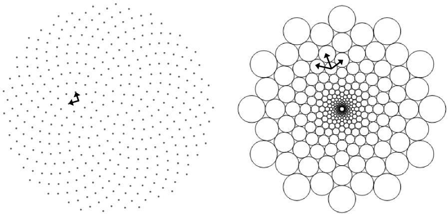
Figure 1: Left: Vogel spiral $\sqrt{n}e^{2\pi in/(1+\gamma_{1})}$ ($n>0$: integer) and images of the lattice shortest vectors (arrows) that indicate the directions of parastichies, Right: Doyle spiral of type $(12,24)$. This article deals with a generalization which includes both cases.

The generated patterns can be regarded as the image of the lattice with the basis:

$$\begin{pmatrix}1\\ 0\end{pmatrix},\begin{pmatrix}\varphi\\ \epsilon_{0}\end{pmatrix},\quad\varphi=\frac{1}{1+\gamma_{1}},\ \epsilon_{0}:\text{constant.}$$ (1)

Variations of the Vogel spiral can be created by substituting different $\varphi$ [29]. While the golden angle method is applicable to surfaces with circular symmetry, it has not been known how to generalize it on general surfaces or manifolds in higher dimensions, maintaining the packing density in a certain range. Akiyama posed the golden angle method for higher dimensions as an open problem [2]. The main goal of this paper is to establish a general theory and a concrete method for that.

As a packing, we shall consider an arrangement of non-overlapping $n$-dimensional balls of the identical radius. Although the case of varying radii is not the scope of this article, the Doyle spiral (Figure 1) has also been addressed as a pattern of parastichies [4] and known as the case of conformal mapping. In fact, the Doyle spiral and the Vogel spiral can be constructed within the same framework (Example 2).

Firstly, for the above goal, we need to determine the optimal lattice of general rank that will be used in our packing method. As shown in (2) of Theorem 1, even in the rank 2 case, the lattice given by (1) is not optimal for bounding the packing density by a larger lower limit.

For any $B_{n}\in GL_{n}({\mathbb{R}})$, let $L(B_{n})$ be the lattices generated by the column vectors of $B_{n}$. The following problem will be discussed in Section 2 for determining the optimal lattices, in particular from known theorems as products of linear forms.

Problem:

Determine the lattice basis $B\in GL_{n}({\mathbb{R}})$ with $\Delta_{n}^{\prime}=\Delta^{\prime}(L(B))$.

$$\Delta_{n}^{\prime} := \sup_{B\in GL_{n}({\mathbb{R}}),}\Delta^{\prime}(L(B)),$$ (2)

$$\Delta^{\prime}(L(B)) := \inf_{D\in GL_{n}({\mathbb{R}})\text{: diagonal}}\Delta(L(DB)).$$

The answer for the above problem enables us to expand the scope of the golden angle method to higher dimensions. The packings densities of the obtained aperiodic packings are bounded below approximately by $\Delta_{n}^{\prime}$ for each dimension $n$:

$$\Delta_{2}^{\prime}=\frac{\pi}{2\sqrt{5}}\approx 0.702, \Delta_{3}^{\prime}=\frac{\sqrt{3}\pi}{14}\approx 0.389,$$

$$\Delta_{4}^{\prime}\geq\frac{\pi^{2}}{10\sqrt{29}}\approx 0.183, \Delta_{5}^{\prime}\geq\frac{5\sqrt{5}\pi^{2}}{12\cdot 11^{2}}\approx 0.076.$$

In addition to the lattices, a map $f({\mathbf{x}})=(f_{1},\ldots,f_{N})$ from an open subset ${\mathfrak{D}}\subset{\mathbb{R}}^{n}$ to ${\mathbb{R}}^{N}$ ($n\leq N$) with the Jacobian matrix $Df({\mathbf{x}})=(f_{i}/\partial x_{j})_{i,j}$ satisfying ($\star$) and ($\star\star$), is used in our packing method. The property ($\star\star$) makes the Voronoi diagram of the generated packing have Voronoi cells of approximately equal volume.

• ${\hskip 1.42262pt{}^{t}(Df)}Df$ is an invertible diagonal matrix for any ${\mathbf{x}}\in{\mathfrak{D}}$ (diagonalizable).

• $\det{\hskip 1.42262pt{}^{t}(Df)}Df=c^{2}$ for some constant $c\neq 0$ (volume-preserving).

For a fixed pair of a map $f:{\mathfrak{D}}\rightarrow{\mathbb{R}}^{N}$ and a lattice $L\subset{\mathbb{R}}^{n}$, a packing of $f({\mathfrak{D}})$ is provided as $f(L\cap{\mathfrak{D}})$.

($\star$) means that the metric on $f({\mathfrak{D}})\subset{\mathbb{R}}^{N}$ induced from the Euclidean metric of ${\mathbb{R}}^{N}$ is diagonal. In a local sense, diagonalization of the metric is possible for any $C^{\infty}$ Riemannian manifolds of dimensions $n\leq 3$. The case of $n=2$ follows from the existence of conformal metric $\lambda(x,y)(dx^{2}+dy^{2})$, and the case of $n=3$ was proved in [13].

The main purpose of Section 3 is to discuss the system of partial differential equations (PDEs) that provide $f$ satisfying ($\star$), ($\star\star$) for $n=N$, and to present new aperiodic packings obtained by our generalization. The results for the general case $n\leq N$ are summarized in Section 4. In Theorem 2, we prove that any real analytic Riemannian surface has an atlas $\{(U_{\alpha},\varphi_{\alpha})\}_{\alpha\in I}$ such that every $U_{\alpha}$ has the metric our packing method can be applied to. The same is clearly true for $n=1$ in case of piecewise differentiable curves, because ($\star$) and ($\star\star$) means that $f$ is a parametrization of $f({\mathfrak{D}})$ by the arc-length.

Subsequently, a family of the PDE solutions for general dimensions is provided (Theorem 3) to explain the self-similarity observed among the aperiodic packings provided in Section 3. Another family obtained from solutions of the inviscid Burgers equation $u_{t}+uu_{x}=0$, also has the same self-similarity (Example 4).

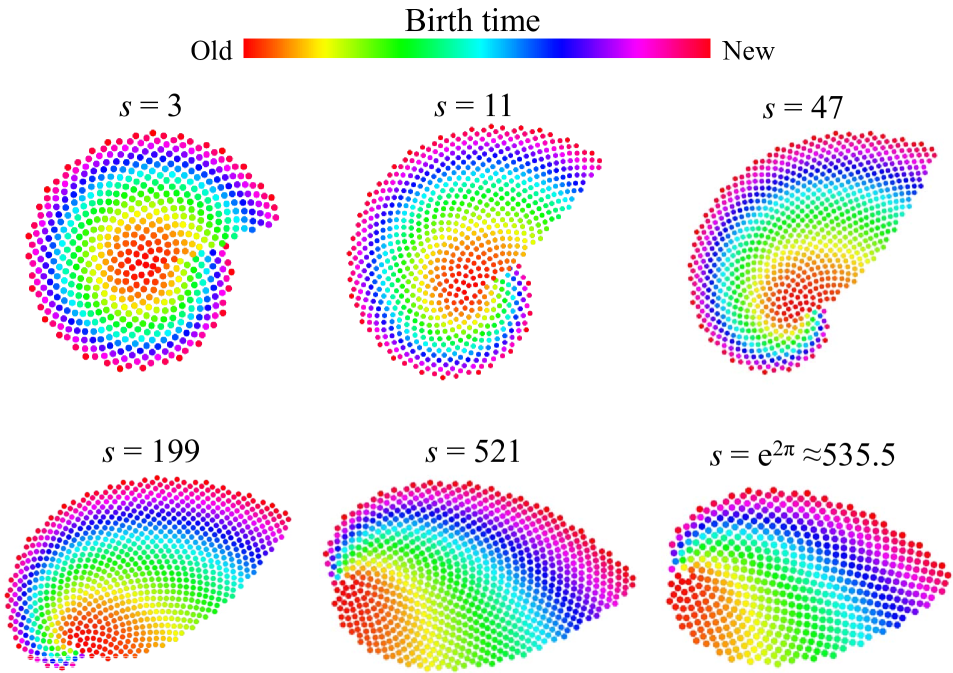
Figure 5: Packing of planes with logarithmic spirals. Each point is colored according to the $y$-value (birth time) of its preimage. The points with the same $y$-value form the identical shape, regardless of $0<y\leq M$. This self-similarity explains their biological shapes. The last $s=e^{2\pi}$ is also the case of an inviscid Burgers solution.

As a motivation for Theorem 3, we remark that the Vogel spiral and the phyllotaxis model can be regarded as a growing disk and a growing cylindrical surface, respectively. This aspect of the golden angle method seems to have been not clear, while it is only applicable to surfaces with circular symmetry. Even after the generalization, the obtained packings still have the following commonly features and an appearance reminiscent of biological growth as seen in Figures 5, 6.

Firstly, the packings presented in this article are the images of lattice points contained in a rectangle ${\mathfrak{D}}$ (or a rectangular parallelepiped for the 3D case), which suggests that there is an inductive way to construct the PDE solutions. Secondly, $f({\mathfrak{D}})$ has a codimension-1 foliation $\{L_{t}\}$ such that any leaves $L_{t}\subset f({\mathfrak{D}})$ are similar to each other in ${\mathbb{R}}^{N}$. More specifically, if the last entry $x_{n}$ is separated so that ${\mathbf{x}}=({\mathbf{x}}_{n-1},x_{n})$ and ${\mathfrak{D}}={\mathfrak{D}}_{2}\times I$ (${\mathfrak{D}}_{2}\subset{\mathbb{R}}^{n-1}$, $I\subset{\mathbb{R}}$), every $f$ can be represented by

$$f({\mathbf{x}})=e^{\alpha(h({\mathbf{x}}))}U(h({\mathbf{x}}))f_{2}({\mathbf{x}}_{n-1})+{\mathbf{v}}_{0}$$ (3)

for some functions $h:{\mathfrak{D}}\rightarrow{\mathbb{R}}$, $\alpha:h({\mathfrak{D}})\rightarrow{\mathbb{R}}$, $U:h({\mathfrak{D}})\rightarrow O(N)$, $f_{2}:{\mathfrak{D}}_{2}\rightarrow{\mathbb{R}}^{N}$ and ${\mathbf{v}}_{0}\in{\mathbb{R}}^{N}$. Thus, if $t=h({\mathbf{x}})$ is considered as the time variable, the image of $\{{\mathbf{x}}\in{\mathfrak{D}}:t=h({\mathbf{x}})\}$ by $f$ has the identical shape as $f_{2}({\mathfrak{D}}_{2})$ for any $t\in I$.

Theorem 3 provides a method to construct $(n+1)$-dimensional Riemannian manifolds with a diagonal and constant-determinant metric from manifolds of dimension $n$ with such a metric. In particular, for dimensions $n=2,3$, Theorem 3 can provide a large family of lattice maps in the form of Eq.(3) that fulfill ($\star$) and ($\star\star$).

Aperiodic packing has a number of applications. When quasicrystals were discovered [34], the Penrose tiling was immediately suggested as a mathematical model of aperiodic structures with a long-range order [22]. More recently, iterative algorithms for generating circle packings on Riemann surfaces have been studied [9], inspired by the Koebe-Andreev-Thurston theorem [19], [3], [37] and the Thurston conjecture proved in [31].

Herein, the golden angle method has been generalized by using volume-preserving maps, instead of conformal maps, based on algebraic properties of certain special lattices.

Methods to color point sets

All the presented packings are 2D or 3D scatter plots displayed by Wolfram Mathematica. The points are colored by either of two methods. The first one colors each point according to the local packing density in its neighborhood. In the considered situation in which the lattice basis $B$ and the map $f$ on ${\mathfrak{D}}\subset{\mathbb{R}}^{n}$ are specified, the local density around $f({\mathbf{x}})$ can be approximated from the packing density of the lattice $L((Df({\mathbf{x}}))B)$. In fact, in some neightborhood ${\mathbf{x}}\in U\subset{\mathfrak{D}}$ with a finite volume, the density of $f(cL(B)\cap U)$ in $f(U)$ converges to that of $cL(Df({\mathbf{x}})B)$ as $c\rightarrow 0$ (Theorem 3).

The second one colors each point, according to its birth time, by considering some $x_{i}$ among ${\mathbf{x}}=(x_{1},\ldots,x_{n})$ as the time when the point $f({\mathbf{x}})$ is generated (e.g., Figure 5). This method allows easy observation of the self-similarity hidden in the image.

Notation and symbols

The continued fractions are represented using squared brackets $[\ ]$ as follows.

$$[a_{0},a_{1},a_{2},\cdots,a_{n},\cdots]:=a_{0}+\frac{1}{a_{1}+}\frac{1}{a_{2}+}\frac{1}{a_{3}+}\cdots\frac{1}{a_{n}+}\cdots.$$

If $[a_{0},a_{1},\ldots]$ is purely periodic, there is an integer $m>0$ such that $a_{m+n}=a_{n}$ for any $n\geq 0$. In such a case, $[a_{0},a_{1},\ldots]$ is abbreviated as $[\overline{a_{0},a_{1},\ldots,a_{m-1}}]$. The $n$’th convergent $p_{n}/q_{n}$ of $\varphi=[a_{0},a_{1},a_{2},\cdots]$ is the ratio of the coprime integers $p_{n}$, $q_{n}$ that satisfy $p_{n}/q_{n}=[a_{0},a_{1},a_{2},\cdots,a_{n}]$.

For any lattice $L\subset{\mathbb{R}}^{n}$ of full rank, we denote the packing density by $\Delta(L)$.

$$\Delta(L) = \frac{{\rm vol}(B(1))(\min\,L)^{n/2}}{2^{n}{\rm vol}({\mathbb{R}}^{n}/L)}=\frac{\pi^{n/2}}{\Gamma(n/2+1)}\frac{(\min\,L)^{n/2}}{2^{n}{\rm vol}({\mathbb{R}}^{n}/L)},$$ (4)

where ${\rm vol}(B(1))$ and ${\rm vol}({\mathbb{R}}^{n}/L)$ are the volumes of the ball with radius 1 in ${\mathbb{R}}^{n}$ and ${\mathbb{R}}^{n}/L$. In addition,

$$\min\,L:=\{{\left\lvert l\right\rvert}^{2}:0\neq l\in L\}.$$ (5)

$B\in GL_{n}({\mathbb{R}})$ is called a basis matrix of $L$, if the columns of $B$ are a basis of $L$. Such a lattice $L$ is also denoted as $L(B)$ explicitly. For any diagonal $D\in GL_{n}({\mathbb{R}})$, the lattice $L(DB)$ is also denoted by $D\cdot L$.

We define the Lagrange number and Markoff spectrum for Theorem 1.

Definition 1.

For any real number $\alpha$, the supremum $\sup M$ of $M$ that fulfills (*) is called the Lagrange number of $\alpha$, and denoted by ${\mathcal{L}}(\alpha)$.

(*)

Infinitely many rationals $p/q$ satisfy ${\left\lvert\alpha-p/q\right\rvert}<\displaystyle\frac{1}{Mq^{2}}$.

The set $\{{\mathcal{L}}(\alpha):\alpha\in{\mathbb{R}}\setminus{\mathbb{Q}}\}$ is called the Lagrange spectrum.

For any irrational $\alpha$, its Lagrange number can be calculated from the continued fraction expansion $\alpha=[a_{0},a_{1},a_{2},\ldots]$ by the following formula (cf. Proposition 1.22, [1]):

$${\mathcal{L}}(\alpha)=\limsup_{n\rightarrow\infty}\left([a_{n+1},a_{n+2},\ldots]+[0,a_{n},a_{n-1},\ldots,a_{1}]\right).$$

For any indefinite binary quadratic form $f(x,y)=ax^{2}+bxy+cy^{2}$ with real coefficients, its discriminant $d(f)$ and minimum $m(f)$ are defined by:

$$d(f) = b^{2}-4ac,$$

$$m(f) = \min\left\{{\left\lvert f(x,y)\right\rvert}:0\neq(x,y)\in{\mathbb{Z}}^{2}\right\}.$$

Definition 2.

The set of ${\mathcal{M}}(f):=\sqrt{d(f)}/m(f)$ of all the indefinite binary quadratic forms over ${\mathbb{R}}$ is the Markoff spectrum.

The Markoff theorem states that the Lagrange spectrum and the Markoff spectrum coincide below 3 [24]. In fact, any indefinite binary quadratic forms $f$ over ${\mathbb{R}}$ with ${\mathcal{M}}(f)<3$, has a root $\alpha$ of $f(x,1)=0$ that fulfills ${\mathcal{M}}(f)={\mathcal{L}}(\alpha)$. Such an $\alpha$ (i.e., $\alpha\in{\mathbb{R}}$ with ${\mathcal{L}}(\alpha)<3$) is a quadratic irrational with the continued fraction expansion $\alpha=[a_{0},\ldots,a_{n},\gamma]$, where $\gamma$ is equal to one of the following $\gamma_{m}$:

$$\gamma_{m}=\frac{m+2u+\sqrt{9m^{2}-4}}{2m},$$ (6)

where $m$ is one of the Markoff numbers $m=1,2,5,13,\ldots$ i.e., positive integers that fulfill the Markoff equation for some integers $m_{1},m_{2}$:

$$m^{2}+m_{1}^{2}+m_{2}^{2}=3mm_{1}m_{2}.$$

The integer $0\leq u\leq m/2$ is the solution of $u^{2}\equiv-1$ mod $m$.

2 Parastichies from a viewpoint of lattice-basis reduction and Markoff theory

Mathematically, parastichies are the images of lines that connect lattice points with the shortest vectors. In order to see this more precisely, it is useful to review Markov theory from a viewpoint of the lattice theory. Although similar results have been known in the study of indefinite quadratic forms, Proposition 1 is a result on the reduction of positive-definite quadratic forms.

Let $\varphi_{1}>0>\varphi_{2}$ be real numbers with the continued fraction expansions:

$$\varphi_{1} = [a_{0},a_{1},a_{2},\cdots,a_{n},\cdots],$$

$$-\varphi_{2}^{-1} = [a_{-1},a_{-2},\cdots,a_{-n},\cdots].$$

The doubly infinite sequence $\{a_{n}\}_{n=-\infty}^{\infty}$ associated with $(\varphi_{1},\varphi_{2})$ is obtained as a result. For simplicity, $\varphi_{1},\varphi_{2}$ are assumed to be irrational. Hence $a_{n}>0$ for any $n\neq 0,-1$.

Let $p_{n}^{(+)}/q_{n}^{(+)}=[a_{0},a_{1},a_{2},\cdots,a_{n}]$, $p_{n}^{(-)}/q_{n}^{(-)}=[a_{-1},a_{-2},a_{-3},\cdots,a_{-n-1}]$ be the $n$’th convergent of $\varphi_{1}$ and $-\varphi_{2}^{-1}$. For $n=-1,-2$, we put:

$$\begin{pmatrix}p_{-1}^{(+)}&p_{-2}^{(+)}\\ q_{-1}^{(+)}&q_{-2}^{(+)}\\ \end{pmatrix}=\begin{pmatrix}p_{-1}^{(-)}&p_{-2}^{(-)}\\ q_{-1}^{(-)}&q_{-2}^{(-)}\\ \end{pmatrix}=\begin{pmatrix}1&0\\ 0&1\end{pmatrix}.$$

If $\varphi_{1}=[\overline{a_{0},a_{1},\ldots,a_{m-1}}]$, the following equality holds for the conjugate $\overline{\varphi_{1}}$ of $\varphi_{1}$ (Lemma 1.28, [1]):

$$-1/\overline{\varphi_{1}}=[\overline{a_{m-1},a_{m-2},\ldots a_{0}}].$$

Therefore, if $\varphi_{2}=\overline{\varphi_{1}}$, $\{a_{n}\}_{n=-\infty}^{\infty}$ is also a periodic sequence.

For any $\epsilon>0$, let $L_{\varphi_{1},\varphi_{2},\epsilon}$ be the lattice with the following basis:

$${\mathbf{b}}_{0}:=\begin{pmatrix}\epsilon^{-1/2}\\ \epsilon^{1/2}\end{pmatrix},\quad{\mathbf{b}}_{-1}:=\begin{pmatrix}-\epsilon^{-1/2}\varphi_{1}\\ -\epsilon^{1/2}\varphi_{2}\end{pmatrix}.$$

A new basis ${\mathbf{b}}_{n},{\mathbf{b}}_{n-1}$ of $L_{\varphi_{1},\varphi_{2},\epsilon}$ can be provided by:

$${\mathbf{b}}_{n} = \begin{cases}p_{n-1}^{(+)}{\mathbf{b}}_{0}+q_{n-1}^{(+)}{\mathbf{b}}_{-1}&\text{if }n>0,\\ (-1)^{n}(q_{-n-2}^{(-)}{\mathbf{b}}_{0}-p_{-n-2}^{(-)}{\mathbf{b}}_{-1})&\text{if }n<-1.\end{cases}$$

In fact, from the definition,

$$\begin{pmatrix}{\mathbf{b}}_{n}&{\mathbf{b}}_{n-1}\end{pmatrix} = \begin{cases}\begin{pmatrix}{\mathbf{b}}_{0}&{\mathbf{b}}_{-1}\end{pmatrix}\begin{pmatrix}p_{n-1}^{(+)}&p_{n-2}^{(+)}\\ q_{n-1}^{(+)}&q_{n-2}^{(+)}\\ \end{pmatrix}&\text{if }n\geq 0,\\ (-1)^{n}\begin{pmatrix}{\mathbf{b}}_{0}&{\mathbf{b}}_{-1}\end{pmatrix}\begin{pmatrix}q_{-n-2}^{(-)}&-q_{-n-1}^{(-)}\\ -p_{-n-2}^{(-)}&p_{-n-1}^{(-)}\\ \end{pmatrix}&\text{if }n\leq 0,\end{cases}$$

$$= \begin{cases}\begin{pmatrix}\epsilon^{-1/2}&0\\ 0&\epsilon^{1/2}\end{pmatrix}\begin{pmatrix}1&-\varphi_{1}\\ 1&-\varphi_{2}\end{pmatrix}\begin{pmatrix}a_{0}&1\\ 1&0\\ \end{pmatrix}\cdots\begin{pmatrix}a_{n-1}&1\\ 1&0\\ \end{pmatrix}&\text{if }n\geq 0,\\ \begin{pmatrix}\epsilon^{-1/2}&0\\ 0&\epsilon^{1/2}\end{pmatrix}\begin{pmatrix}1&-\varphi_{1}\\ 1&-\varphi_{2}\\ \end{pmatrix}\begin{pmatrix}0&1\\ 1&-a_{-1}\\ \end{pmatrix}\cdots\begin{pmatrix}0&1\\ 1&-a_{n}\\ \end{pmatrix}&\text{if }n\leq 0.\end{cases}$$

Hence,

$$\begin{pmatrix}{\mathbf{b}}_{n}&{\mathbf{b}}_{n-1}\end{pmatrix} = \begin{cases}\begin{pmatrix}{\mathbf{b}}_{n-1}&{\mathbf{b}}_{n-2}\end{pmatrix}\begin{pmatrix}a_{n-1}&1\\ 1&0\\ \end{pmatrix}&\text{if }n\geq 1,\\ \begin{pmatrix}{\mathbf{b}}_{n+1}&{\mathbf{b}}_{n}\end{pmatrix}\begin{pmatrix}0&1\\ 1&-a_{n}\\ \end{pmatrix}&\text{if }n\leq-1.\end{cases}$$

Thus, ${\mathbf{b}}_{n}=a_{n-1}{\mathbf{b}}_{n-1}+{\mathbf{b}}_{n-2}$ holds for any $n\in{\mathbb{Z}}$. From $a_{0},a_{-1}\geq 0$, $a_{n}>0$ ($n\neq 0,-1$) and the following, $\{{\mathbf{b}}_{n}\cdot{\mathbf{b}}_{n-1}\}_{n=-\infty}^{\infty}$ increases monotonically:

$${\mathbf{b}}_{n}\cdot{\mathbf{b}}_{n-1}-{\mathbf{b}}_{n-1}\cdot{\mathbf{b}}_{n-2}=a_{n-1}{\mathbf{b}}_{n-1}\cdot{\mathbf{b}}_{n-1}.$$

In addition,

$${\mathbf{b}}_{n}\cdot{\mathbf{b}}_{n-1}=\begin{cases}\epsilon^{-1}q_{n-1}^{(+)}q_{n-2}^{(+)}\left(p_{n-1}^{(+)}/q_{n-1}^{(+)}-\varphi_{1}\right)\left(p_{n-2}^{(+)}/q_{n-2}^{(+)}-\varphi_{1}\right)\\ \hskip 14.22636pt+\epsilon q_{n-1}^{(+)}q_{n-2}^{(+)}\left(p_{n-1}^{(+)}/q_{n-1}^{(+)}-\varphi_{2}\right)\left(p_{n-2}^{(+)}/q_{n-2}^{(+)}-\varphi_{2}\right)&n\geq 0,\\ -\epsilon\varphi_{2}^{2}q_{-n-1}^{(-)}q_{-n-2}^{(-)}\left(p_{-n-1}^{(-)}/q_{-n-1}^{(-)}+\varphi_{2}^{-1}\right)\left(p_{-n-2}^{(-)}/q_{-n-2}^{(-)}+\varphi_{2}^{-1}\right)\\ \hskip 14.22636pt-\epsilon^{-1}\varphi_{1}^{2}q_{-n-1}^{(-)}q_{-n-2}^{(-)}\left(p_{-n-1}^{(-)}/q_{-n-1}^{(-)}+\varphi_{1}^{-1}\right)\left(p_{-n-2}^{(-)}/q_{-n-2}^{(-)}+\varphi_{1}^{-1}\right)&n\leq 0.\end{cases}$$

The first terms converge to $0$ as $n\rightarrow\infty$. The second terms diverge owing to $q_{n}^{(+)}\rightarrow\infty$ and $q_{-n}^{(-)}\rightarrow\infty$ ($n\rightarrow\infty$). Hence, $\displaystyle\lim_{n\rightarrow\infty}{\mathbf{b}}_{n}\cdot{\mathbf{b}}_{n-1}=\infty$. Similarly, $\displaystyle\lim_{n\rightarrow-\infty}{\mathbf{b}}_{n}\cdot{\mathbf{b}}_{n-1}=-\infty$ is obtained.

The term superbasis was first used in [10] to explain the Selling reduction [33].

Definition 3.

For any lattice $L$ of rank 2, a basis $u_{1},u_{2}\in L$ and $u_{3}=-u_{1}-u_{2}$ are a Selling-reduced superbasis, if $u_{1},u_{2},u_{3}$ satisfy $u_{1}\cdot u_{2}\leq 0$, $u_{1}\cdot u_{3}\leq 0$, and $u_{2}\cdot u_{3}\leq 0$.

Proposition 1.

For any $\varphi_{1}>0>\varphi_{2}$ and $\epsilon>0$, suppose that a lattice $L_{\varphi_{1},\varphi_{2},\epsilon}$ and its basis vectors ${\mathbf{b}}_{n}$ ($n\in{\mathbb{Z}}$) are defined as above. Let $N$ be the integer that fulfills $n\geq N\Leftrightarrow{\mathbf{b}}_{n}\cdot{\mathbf{b}}_{n-1}\geq 0$, and $1\leq d\leq a_{N-1}$ be the smallest integer that satisfies $(d{\mathbf{b}}_{N-1}+{\mathbf{b}}_{N-2})\cdot{\mathbf{b}}_{N-1}\geq 0$. In this case, the following $u_{1},u_{2},u_{3}$ are a Selling reduced superbasis of $L_{\varphi_{1},\varphi_{2},\epsilon}$.

$$u_{1}:={\mathbf{b}}_{N-1},\quad u_{2}:=(d-1){\mathbf{b}}_{N-1}+{\mathbf{b}}_{N-2},\quad u_{3}:=-u_{1}-u_{2}=-(d{\mathbf{b}}_{N-1}+{\mathbf{b}}_{N-2}).$$

In addition, one of the following holds:

1. ${\left\lvert u_{1}\right\rvert}<{\left\lvert u_{2}\right\rvert},{\left\lvert u_{3}\right\rvert}$.

2. ${\left\lvert u_{2}\right\rvert}\leq{\left\lvert u_{1}\right\rvert}<{\left\lvert u_{3}\right\rvert}$. In this case, $d=1$, $u_{2}={\mathbf{b}}_{N-2}$.

3. ${\left\lvert u_{3}\right\rvert}\leq{\left\lvert u_{1}\right\rvert}<{\left\lvert u_{2}\right\rvert}$. In this case, $d=a_{N-1}$, $u_{3}=-{\mathbf{b}}_{N}$.

4. ${\left\lvert u_{2}\right\rvert},{\left\lvert u_{3}\right\rvert}\leq{\left\lvert u_{1}\right\rvert}$. In this case, $d=a_{N-1}=1$ and $u_{2}={\mathbf{b}}_{N-2}$, $u_{3}=-{\mathbf{b}}_{N}$.

In particular, one of ${\mathbf{b}}_{N-2},{\mathbf{b}}_{N-1}$, or ${\mathbf{b}}_{N}$ is the shortest vector of $L_{\varphi_{1},\varphi_{2},\epsilon}$.

Proof.

From the choice of $N$, ${\mathbf{b}}_{N}\cdot{\mathbf{b}}_{N-1}\geq 0$ and ${\mathbf{b}}_{N-1}\cdot{\mathbf{b}}_{N-2}<0$ hold. Since $(x{\mathbf{b}}_{N-1}+{\mathbf{b}}_{N-2})\cdot{\mathbf{b}}_{N-1}$ monotonically increases as a function of $x$, there is an integer $1\leq d\leq a_{N-1}$ as stated above.

We shall show that $u_{1},u_{2},u_{3}$ are a Selling-reduced superbasis; clearly, $u_{1},u_{2}$ are a basis of $L_{\varphi_{1},\varphi_{2},\epsilon}$. From the definition, $u_{1}\cdot u_{2}<0$ and $u_{1}\cdot u_{3}\leq 0$. Hence, we only need to show that $u_{2}\cdot u_{3}\leq 0$. For the proof, $N\geq 1$ may be assumed; in fact, for any integer $-M<N$, $\begin{pmatrix}{\mathbf{b}}_{0}&{\mathbf{b}}_{-1}\end{pmatrix}$ can be replaced with $\begin{pmatrix}{\mathbf{b}}_{-M}&{\mathbf{b}}_{-M-1}\end{pmatrix}$, by replacing $\varphi_{1},\varphi_{2}$ with $[a_{-M},a_{-M+1},\ldots,]$, $-[0,a_{-M-1},a_{-M-2},\ldots]$, and changing $\epsilon$ accordingly. As a result, $N$ can be set to a positive integer.

From the process of the continued fraction expansion, $a_{N}$ ($N\geq 1$) is the largest integer among all the $c$’s for which the following two have different signatures:

$$\frac{p_{N-1}^{(+)}}{q_{N-1}^{(+)}}-\varphi_{1} = [a_{0},a_{1},\ldots,a_{N-1}]-\varphi_{1},$$

$$\frac{cp_{N-1}^{(+)}+p_{N-2}^{(+)}}{cq_{N-1}^{(+)}+q_{N-2}^{(+)}}-\varphi_{1} = [a_{0},a_{1},\ldots,a_{N-1},c]-\varphi_{1}.$$

In particular, the following two have the same signature for any $1\leq r\leq a_{N}$:

$$\frac{(r-1)p_{N-1}^{(+)}+p_{N-2}^{(+)}}{(r-1)q_{N-1}^{(+)}+q_{N-2}^{(+)}}-\varphi_{1} = [a_{0},a_{1},\ldots,a_{N-1},r-1]-\varphi_{1},$$

$$\frac{rp_{N-1}^{(+)}+p_{N-2}^{(+)}}{rq_{N-1}^{(+)}+q_{N-2}^{(+)}}-\varphi_{1} = [a_{0},a_{1},\ldots,a_{N-1},r]-\varphi_{1}.$$

Thus, $u_{2}\cdot u_{3}\leq 0$ is obtained from the following:

$$-u_{2}\cdot u_{3} = ((d-1)q_{N-1}^{(+)}+q_{N-2}^{(+)})(dq_{N-1}^{(+)}+q_{N-2}^{(+)})$$

$$\times\begin{Bmatrix}\epsilon^{-1}\left(\frac{(d-1)p_{N-1}^{(+)}+p_{N-2}^{(+)}}{(d-1)q_{N-1}^{(+)}+q_{N-2}^{(+)}}-\varphi_{1}\right)\left(\frac{dp_{N-1}^{(+)}+p_{N-2}^{(+)}}{dq_{N-1}^{(+)}+q_{N-2}^{(+)}}-\varphi_{1}\right)+\epsilon\left(\frac{(d-1)p_{N-1}^{(+)}+p_{N-2}^{(+)}}{(d-1)q_{N-1}^{(+)}+q_{N-2}^{(+)}}-\varphi_{2}\right)\left(\frac{dp_{N-1}^{(+)}+p_{N-2}^{(+)}}{dq_{N-1}^{(+)}+q_{N-2}^{(+)}}-\varphi_{2}\right)\end{Bmatrix}.$$

Therefore, $u_{1},u_{2},u_{3}$ is Selling reduced, which implies that one of $u_{1},u_{2},u_{3}$ is the shortest vector of $L$.

As for the second statement, the following equation is obtained in a similar way as the above:

$${\left\lvert u_{2}\right\rvert}\leq{\left\lvert u_{1}\right\rvert} \Leftrightarrow -(u_{2}-u_{1})\cdot u_{3}\leq 0$$ (7)

$$\Rightarrow \left(\frac{(d-2)p_{N-1}^{(+)}+p_{N-2}^{(+)}}{(d-2)q_{N-1}^{(+)}+q_{N-2}^{(+)}}-\varphi_{1}\right)\left(\frac{dp_{N-1}^{(+)}+p_{N-2}^{(+)}}{dq_{N-1}^{(+)}+q_{N-2}^{(+)}}-\varphi_{1}\right)<0,$$

$${\left\lvert u_{3}\right\rvert}\leq{\left\lvert u_{1}\right\rvert} \Leftrightarrow -u_{2}\cdot(u_{3}-u_{1})\leq 0$$ (8)

$$\Rightarrow \left(\frac{(d+1)p_{N-1}^{(+)}+p_{N-2}^{(+)}}{(d+1)q_{N-1}^{(+)}+q_{N-2}^{(+)}}-\varphi_{1}\right)\left(\frac{(d-1)p_{N-1}^{(+)}+p_{N-2}^{(+)}}{(d-1)q_{N-1}^{(+)}+q_{N-2}^{(+)}}-\varphi_{1}\right)<0.\quad\quad$$

Because the values in the parentheses of Eq.(7) have different signatures owing to the inequality, ${\left\lvert u_{2}\right\rvert}\leq{\left\lvert u_{1}\right\rvert}$ implies $d=1$. Similarly, ${\left\lvert u_{3}\right\rvert}\leq{\left\lvert u_{1}\right\rvert}$ implies $d=a_{N-1}$. ∎

∎

The determination of $\Delta_{n}^{\prime}$, $\Delta^{\prime}(L(B_{n}))$ is equivalent to that of the $\lambda_{n}^{\prime},\lambda^{\prime}(B_{n})$.

$$\lambda_{n}^{\prime} := \sup_{B_{n}\in GL_{n}({\mathbb{R}}),\det B_{n}=\pm 1}\lambda^{\prime}(B_{n}),$$

$$\lambda^{\prime}(B_{n}) := \inf_{{D\in GL_{n}({\mathbb{R}})\text{: diagonal}}\atop{\det D=\pm 1}}\min\,L(DB_{n}).$$

In fact, for any $B_{n}\in GL_{n}({\mathbb{R}})$ with the determinant $\pm 1$,

$$\Delta^{\prime}(L(B_{n})) = \frac{(\pi\lambda^{\prime}(B_{n})/4)^{n/2}}{\Gamma(n/2+1)}.$$ (9)

The determination of $\lambda^{\prime}_{n}$ and $\lambda^{\prime}(B_{n})$ is boiled down to the problem about the products of linear forms $\lambda_{n}$ and $\lambda(B_{n})$.

$$\lambda_{n} := \sup_{{B_{n}=(b_{ij})\in GL_{n}({\mathbb{R}}),}\atop{\det B=\pm 1}}\lambda(B_{n}),$$ (10)

$$\lambda(B_{n}) := \inf_{0\neq(x_{1},\ldots,x_{n})\in{\mathbb{Z}}^{n}}{\left\lvert\prod_{i=1}^{n}(b_{i1}x_{1}+\cdots+b_{in}x_{n})\right\rvert}.$$

Lemma 1.

1. For any $B=(b_{ij})\in GL_{n}({\mathbb{R}})$ with $\lambda(B_{n})\neq 0$, the following equality holds:

   $$\lambda^{\prime}(B_{n})=n\left(\lambda(B_{n})\right)^{2/n}.$$ (11)

2. If a totally real algebraic number field $K$ of degree $n$ has discriminant $d_{K}$, then, $\lambda_{n}\geq d_{K}^{-1/2}$. Furthermore, for each $n$, some $B_{n}$ attains the supremum $\Delta_{n}^{\prime}$, and

   $$\Delta^{\prime}_{n} = \frac{(\pi\lambda_{n}^{\prime}/4)^{n/2}}{\Gamma(n/2+1)}=\frac{(\pi n/4)^{n/2}\lambda_{n}}{\Gamma(n/2+1)}\geq\frac{(\pi n/4)^{n/2}d_{K}^{-1/2}}{\Gamma(n/2+1)}.$$

Proof.

1. From the inequality of arithmetic and geometric means, the part $\geq$ is proved since we have the following:

   $$\lambda^{\prime}(B_{n}) = \inf_{{d_{1},\ldots,d_{n}\in{\mathbb{R}},\ d_{1}\cdots d_{n}=\pm 1,}\atop{0\neq(x_{1},\ldots,x_{n})\in{\mathbb{Z}}^{n}}}\sum_{i=1}^{n}d_{i}^{2}(b_{i1}x_{1}+\cdots+b_{in}x_{n})^{2},$$

   $$\lambda(B_{n}) = \inf_{0\neq(x_{1},\ldots,x_{n})\in{\mathbb{Z}}^{n}}{\left\lvert\prod_{i=1}^{n}(b_{i1}x_{1}+\cdots+b_{in}x_{n})\right\rvert}.$$

   Furthermore, $>$ is impossible, because if ${\left\lvert\prod_{i=1}^{n}(b_{i1}x_{1}+\cdots+b_{in}x_{n})\right\rvert}=v$ for some $0\neq(x_{1},\ldots,x_{n})\in{\mathbb{Z}}^{n}$, the left-hand side of Eq.(11) cannot be more than $nv^{2/n}$, which is seen by putting $d_{i}={\left\lvert v^{1/n}/(b_{i1}x_{1}+\cdots+b_{in}x_{n})\right\rvert}$.

2. Let $\sigma_{1},\ldots,\sigma_{n}$ be distinct embeddings of $K$ into ${\mathbb{C}}$ over ${\mathbb{Q}}$, $b_{1},\ldots,b_{n}$ be a basis of the ring ${\mathfrak{o}}_{K}$ of integers of $K_{n}$ over ${\mathbb{Z}}$, and $B_{n}\in GL_{n}({\mathbb{R}})$ be the matrix with $b_{j}^{\sigma_{i}}$ in the $(i,j)$-entry. From ${\left\lvert\det B_{n}\right\rvert}=\sqrt{d_{K}}$ and $\displaystyle\min_{0\neq\alpha\in{\mathfrak{o}}_{K}}\sigma_{1}(\alpha)\cdots\sigma_{n}(\alpha)=1$, the following is obtained:

   $$\lambda_{n}\geq\lambda(d_{K}^{-1/2n}B_{n})=d_{K}^{-1/2}.$$

   This implies $\lambda_{n}>0$, namely, the following star body is finite type.

   $$\{(x_{1},\ldots,x_{n})\in{\mathbb{R}}^{n}:{\left\lvert x_{1}\cdots x_{n}\right\rvert}\leq 1\}.$$

   Hence, $\lambda(B_{n})=\lambda_{n}$ holds for some $B_{n}\in GL_{n}({\mathbb{R}})$ with $\det B_{n}=\pm 1$ (Theorem 9 of $\S$17, chap.3 in [16]). For such a $B_{n}$, $\lambda^{\prime}(B_{n})=\lambda_{n}^{\prime}$ and $\Delta^{\prime}(L(B_{n}))=\Delta_{n}^{\prime}$ hold owing to Eqs.(9) and (11). The last inequality is also clear. ∎

∎

The relation between Markoff theory and phyllotaxis was not clarified until very recently [6]. Theorem 1 of [6] handles a special case of our Eq.(12), as their growth capacity is a constant multiple of the packing density. Markoff theory can give us more insights. As seen in (2) of Theorem 1, the golden lattice given by $B_{2}$ is more optimal than the lattice by Eq.(1) that has been used for the golden angle method.

Theorem 1.

1. For $n=2$–$5$, let $B_{n}\in GL_{n}({\mathbb{R}})$ be the matrix with $b_{j}^{\sigma_{i}}$ in each $(i,j)$-entry, where $\sigma_{1},\ldots,\sigma_{n}$ are all the embeddings of the following $K_{n}$ into ${\mathbb{C}}$ over ${\mathbb{Q}}$, and $b_{1},\ldots,b_{n}$ are a basis of the ring of integers of the fields $K_{n}$ as a ${\mathbb{Z}}$-module.

   • $K_{2}={\mathbb{Q}}(\zeta_{5}+\zeta_{5}^{-1})$, $\zeta_{5}=e^{2\pi\sqrt{-1}/5}$,

   • $K_{3}={\mathbb{Q}}(\zeta_{7}+\zeta_{7}^{-1})$, $\zeta_{7}=e^{2\pi\sqrt{-1}/7}$,

   • $K_{4}={\mathbb{Q}}(\sqrt{7+2\sqrt{5}})$,

   • $K_{5}={\mathbb{Q}}(\zeta_{11}+\zeta_{11}^{-1})$, $\zeta_{11}=e^{2\pi\sqrt{-1}/11}$,

   For the above $B_{n}$, the following hold:

   $$\Delta_{2}^{\prime}=\Delta^{\prime}(L(B_{2}))=\frac{\pi}{2\sqrt{5}}\approx 0.702, \Delta_{3}^{\prime}=\Delta^{\prime}(L(B_{3}))=\frac{\sqrt{3}\pi}{14}\approx 0.389,$$

   $$\Delta_{4}^{\prime}\geq\Delta^{\prime}(L(B_{4}))=\frac{\pi^{2}}{10\sqrt{29}}\approx 0.183, \Delta_{5}^{\prime}\geq\Delta^{\prime}(L(B_{5}))=\frac{5\sqrt{5}\pi^{2}}{12\cdot 11^{2}}\approx 0.076.$$

   (For comparison, the packing density of the densest lattice packings are $\pi/2\sqrt{3}\approx 0.907$ for $n=2$, $\pi/3\sqrt{2}\approx 0.740$ [14] for $n=3$, $\pi^{2}/16\approx 0.617$ [20] for $n=4$, and $\pi^{2}/15\sqrt{2}\approx 0.465$ [20] for $n=5$.)

2. For any distinct $\varphi_{1},\varphi_{2}\in{\mathbb{R}}\setminus{\mathbb{Q}}$, let $L_{\varphi_{1},\varphi_{2}}$, $L_{\varphi_{1},\varphi_{2},\epsilon}$ be the lattices $L(B_{1})$, $L(B_{\epsilon})$ generated by the column vectors of the following matrices:

   $$B_{1}=\begin{pmatrix}1&-\varphi_{1}\\ 1&-\varphi_{2}\end{pmatrix},\quad B_{\epsilon}=\begin{pmatrix}\epsilon^{-1/2}&0\\ 0&\epsilon^{1/2}\end{pmatrix}\begin{pmatrix}1&-\varphi_{1}\\ 1&-\varphi_{2}\end{pmatrix}.$$

   Then,

   $$\displaystyle\liminf_{\epsilon\rightarrow+0}\Delta\left(L_{\varphi_{1},\varphi_{2},\epsilon}\right) = \frac{\pi}{2{\mathcal{L}}(\varphi_{1})},$$ (12)

   $$\Delta^{\prime}(L_{\varphi_{1},\varphi_{2}})=\displaystyle\inf_{\epsilon}\Delta\left(L_{\varphi_{1},\varphi_{2},\epsilon}\right) = \displaystyle\frac{\pi}{2{\mathcal{M}}(f)},$$ (13)

   where ${\mathcal{L}}(\varphi_{1})$ is the Lagrange number of $\varphi_{1}$, and ${\mathcal{M}}(f):=\sqrt{d(f)}/m(f)$ is the element of the Markoff spectrum that corresponds to the quadratic form $f(x,y):=(x-\varphi_{1}y)(x-\varphi_{2}y)$.

Remark 1.

Eq.(12) does not hold for any rational $\varphi_{1}$, because ${\mathcal{L}}(\varphi_{1})=0$ if $\varphi_{1}\in{\mathbb{Q}}$ (Corollary 1.2, [1]).

Remark 2.

When $B$ is as in (1) i.e., the rows are conjugate of each other, the product ${\left\lvert\prod_{i=1}^{n}(b_{i1}x_{1}+\cdots+b_{in}x_{n})\right\rvert}=v$ is called a norm form. It is conjectured that for $n\geq 3$, $\lambda(B_{n})>0$ implies that $B_{n}$ is a norm form [11].

Remark 3.

The upper bounds $\lambda_{4}\leq 3/(20\sqrt{5})$ [40] and $\lambda_{5}\leq 1/57.02$ [15] are also known. Therefore, $\Delta_{4}^{\prime}\leq 3\pi^{2}/(40\sqrt{5})\approx 0.331$ and $\Delta_{5}^{\prime}\leq 5\sqrt{5}\pi^{2}/(12\cdot 57.02)\approx 0.161$.

Proof.

1. This part is an immediate consequence of Lemma 1 and the known results: $\lambda_{2}=1/\sqrt{5}$ [20], [23], $\lambda_{3}=1/7$ [12], $\lambda_{4}\geq 1/5\sqrt{29}$ [26] and $\lambda_{5}\geq 11^{-2}$ [18]. The lower bounds for $\lambda_{4},\lambda_{5}$ are from the smallest discriminants among all the totally real quartic and quintic fields.

2. As a result of (2) of Lemma 1, Eq.(13) is obtained as follows:

   $$\Delta^{\prime}(L_{\varphi_{1},\varphi_{2}})=\frac{\pi\lambda(B_{1})}{2{\left\lvert\det B_{1}\right\rvert}}=\frac{\pi\displaystyle\inf_{0\neq(x_{1},\ldots,x_{n})\in{\mathbb{Z}}^{n}}f(x,y)}{2{\left\lvert\varphi_{1}-\varphi_{2}\right\rvert}}=\frac{\pi m(f)}{2\sqrt{d(f)}}=\frac{\pi}{2{\mathcal{M}}(f)}.$$

   Eq.(12) is proved as follows; $\varphi_{1}>0>\varphi_{2}$ may be assumed, by replacing $B_{\epsilon}$ with $DB_{\epsilon}g$ for some for some diagonal $D\in GL_{2}({\mathbb{R}})$ and $g\in GL_{2}({\mathbb{Z}})$. This replaces each $\varphi_{i}$ by a linear fractional transformation of $\varphi_{i}$. Hence, it does not change their Lagrange numbers.

   From Proposition 1, for sufficiently small $\epsilon>0$, the shortest vector of $L_{\varphi_{1},\varphi_{2},\epsilon}$ is equal to $p_{N}^{(+)}{\mathbf{b}}_{1}-q_{N}^{(+)}{\mathbf{b}}_{2}$ using the $N$’th convergent $p_{N}^{(+)}/q_{N}^{(+)}$of $\varphi_{1}$. Furthermore, the following is proved as in Lemma 1.

   $$\displaystyle\liminf_{\epsilon\rightarrow+0}\min L_{\varphi_{1},\varphi_{2},\epsilon} = \liminf_{\epsilon\rightarrow+0}\inf_{N>0}\{\epsilon^{-1}(p_{N}^{(+)}-q_{N}^{(+)}\varphi_{1})^{2}+\epsilon(p_{N}^{(+)}-q_{N}^{(+)}\varphi_{2})^{2}\}$$

   $$= 2\liminf_{N\rightarrow\infty}{\left\lvert(p_{N}^{(+)}-q_{N}^{(+)}\varphi_{1})(p_{N}^{(+)}-q_{N}^{(+)}\varphi_{2})\right\rvert}$$

   $$= 2{\left\lvert\varphi_{1}-\varphi_{2}\right\rvert}\liminf_{N\rightarrow\infty}{\left\lvert q_{N}^{(+)}(p_{N}^{(+)}-q_{N}^{(+)}\varphi_{1})\right\rvert}$$

   $$= \frac{2{\left\lvert\varphi_{1}-\varphi_{2}\right\rvert}}{\limsup_{N\rightarrow\infty}\ell_{N}(\varphi_{1})},\quad(\textit{cf.\ }\text{proof of Proposition1.22 of \cite[cite]{[\@@bibref{}{Aigner2013}{}{}]}})$$

   $$\ell_{n}(\varphi_{1}) := [a_{n+1},a_{n+2},\ldots]+[0,a_{n},a_{n-1},\ldots,a_{1}].$$

   Thus, Eq.(12) is proved as follows:

   $$\liminf_{\epsilon\rightarrow+0}\Delta\left(L_{\varphi_{1},\varphi_{2},\epsilon}\right)=\frac{\pi}{2\limsup_{N\rightarrow\infty}\ell_{N}(\varphi_{1})}=\frac{\pi}{2{\mathcal{L}}(\varphi)}.$$

   ∎

∎

As an immediate consequence of Theorem 1, it is possible to improve the packing around the origin of the Vogel spiral by using the optimal lattice basis $B_{2}$ in Theorem 1 (Figure 2). More obvious examples will be provided in Figure 4 of Section 3.2.

Figure 2: Original Vogel spiral (left) and a packing obtained from the lattice basis $B_{2}$ in Theorem 1 (right).

Example 1 (Vogel spirals for quadratic irrationals $\varphi$ with ${\mathcal{L}}(\varphi)<3$).

The $\gamma_{m}$ defined by Eq.(6) has the Lagrange number ${\mathcal{L}}(\gamma_{m})=\sqrt{9-4/m^{2}}$. Hence, the basis matrix ${\mathcal{B}}_{m}=\begin{pmatrix}1&-\gamma_{m}\\ 1&-\overline{\gamma}_{m}\end{pmatrix}$ fulfills the following for any Markoff number $m$.

$$\Delta^{\prime}(L({\mathcal{B}}_{m}))=\frac{\pi}{2{\mathcal{L}}(\gamma_{m})}=\frac{\pi}{2\sqrt{9-4/m^{2}}}>\frac{\pi}{6}\approx 0.5236.$$

The quadratic irrationals with the smallest Lagrange numbers are $\gamma_{1}=(1+\sqrt{5})/2=[\overline{1}]$, $\gamma_{2}=1+\sqrt{2}=[\overline{2}]$, $\gamma_{5}=(9+\sqrt{221})/10=[\overline{2,2,1,1}]$. For each $m=1,2,5$, the packing density of $L(D{\mathcal{B}}_{m})$ is not less than the following value, regardless of the diagonal $D\in GL_{2}({\mathbb{R}})$:

$$\Delta^{\prime}(L({\mathcal{B}}_{1})) = \frac{\pi}{2\sqrt{5}}\approx 0.7025,$$

$$\Delta^{\prime}(L({\mathcal{B}}_{2})) = \frac{\pi}{4\sqrt{2}}\approx 0.5554,$$

$$\Delta^{\prime}(L({\mathcal{B}}_{5})) = \frac{5\pi}{2\sqrt{221}}\approx 0.5283.$$

The lattice map $f$ used to obtain Figure 2 will be explained in Example 5.

3 Lattice maps for packing of the Euclidean spaces

In this section, it is assumed that $n=N$, and $f({\mathbf{x}})=(f_{1}({\mathbf{x}}),\ldots,f_{n}({\mathbf{x}}))\in C^{3}({\mathfrak{D}},{\mathbb{R}}^{n})$ defined on open subset ${\mathfrak{D}}\subset{\mathbb{R}}^{n}$, satisfies the properties ($\star$), ($\star\star$):

• For any ${\mathbf{x}}\in{\mathfrak{D}}$, there are an orthogonal matrix $U({\mathbf{x}})$ of degree $n$ and a diagonal matrix $\Phi({\mathbf{x}})$ with the diagonal entries $\phi_{i}({\mathbf{x}})>0$ ($i=1,\ldots,n$) that satisfy the following:

  $$Df({\mathbf{x}}):=\begin{pmatrix}\partial f_{1}/\partial x_{1}&\cdots&\partial f_{1}/\partial x_{n}\\ \vdots&&\vdots\\ \partial f_{N}/\partial x_{1}&\cdots&\partial f_{N}/\partial x_{n}\\ \end{pmatrix}=U({\mathbf{x}})\Phi({\mathbf{x}}).$$

• $\det\Phi({\mathbf{x}})=c$ for some constant $c>0$.

After deriving the system of the PDEs for the above $\Phi({\mathbf{x}})$ and $U({\mathbf{x}})$ in Proposition 2, a family of the PDE solutions are provided by using solutions of inviscid Burgers equation (Section 3.1) and separation of variables (Section 3.2).

3.1 System of PDEs and solutions provided by inviscid Burgers equation

First, only ($\star$) is assumed. The constraint ($\star\star$) will not be used until Example 3. Since $f({\mathbf{x}})\in C^{3}({\mathfrak{D}},{\mathbb{R}}^{n})$ and the Jacobian matrix $Df({\mathbf{x}})$ fulfills ${\hskip 1.42262pt{}^{t}(Df)}Df=\Phi({\mathbf{x}})^{2}$, $\phi_{1}({\mathbf{x}}),\ldots,\phi_{n}({\mathbf{x}})$ are $C^{2}$ functions. Let $A_{k}({\mathbf{x}})$ be the matrix defined by $A_{k}({\mathbf{x}}):=U({\mathbf{x}})^{-1}(U({\mathbf{x}}))_{x_{k}}$. From $({\hskip 1.42262pt{}^{t}U}U)_{x_{k}}=O$ and $(U_{x_{k}})_{x_{j}}=(U_{x_{j}})_{x_{k}}$, the following are obtained:

• ${\hskip 1.42262pt{}^{t}A}_{k}+A_{k}=O$.

• $A_{j}A_{k}-A_{k}A_{j}=(A_{j})_{x_{k}}-(A_{k})_{x_{j}}.$

The following theorem specifies the diagonal entries of $\Phi({\mathbf{x}})$ as a solution of second-order PDEs.

Proposition 2.

Let ${\mathfrak{D}}\subset{\mathbb{R}}^{n}$ be a simply-connected open subset. The $\phi_{1}({\mathbf{x}}),\ldots,\phi_{n}({\mathbf{x}})$ that fulfill ($\star$) for some $f\in C^{3}({\mathfrak{D}},{\mathbb{R}}^{n})$, are provided by solving the following PDEs:

$$\phi_{i}^{-1}(\phi_{i})_{x_{k}}(\phi_{j})_{x_{i}}+\phi_{k}^{-1}(\phi_{k})_{x_{i}}(\phi_{j})_{x_{k}}=(\phi_{j})_{x_{i}x_{k}} (1\leq i,j,k\leq n:\text{distinct}),\quad\quad$$ (14)

$$\left(\phi_{k}^{-1}(\phi_{j})_{x_{k}}\right)_{x_{k}}+\left(\phi_{j}^{-1}(\phi_{k})_{x_{j}}\right)_{x_{j}}=-\displaystyle\sum_{i\neq j,k}\phi_{i}^{-2}(\phi_{k})_{x_{i}}(\phi_{j})_{x_{i}} (1\leq j,k\leq n:\text{distinct}).\quad\quad$$ (15)

For fixed $\Phi({\mathbf{x}})$, the matrix $A_{k}=\left(a_{ij}^{(k)}\right)$ ($k=1,\ldots,n$) that satisfy the above (a) and (b) are provided by:

$$A_{k}={\hskip 1.42262pt{}^{t}{\mathbf{e}}_{k}}{\mathbf{c}}_{k}-{\hskip 1.42262pt{}^{t}{\mathbf{c}}_{k}}{\mathbf{e}}_{k},$$ (16)

where ${\mathbf{c}}_{k}:=\left(\phi_{1}^{-1}(\phi_{k})_{x_{1}},\ldots,\phi_{n}^{-1}(\phi_{k})_{x_{n}}\right)$ and ${\mathbf{e}}_{k}$ is the unit vector with 1 in the $k$’th entry. $U({\mathbf{x}})\in O(n)$ is obtained by solving $U_{x_{k}}=UA_{k}$ ($k=1,\ldots,n$).

Proof.

If such an $f$ exists, from $((f_{i})_{x_{j}})_{x_{k}}=((f_{i})_{x_{k}})_{x_{j}}$, $\phi_{1}({\mathbf{x}}),\ldots,\phi_{n}({\mathbf{x}})$ and $U({\mathbf{x}})=\begin{pmatrix}{\mathbf{u}}_{1}({\mathbf{x}})&\cdots&{\mathbf{u}}_{n}({\mathbf{x}})\end{pmatrix}$ satisfy:

$$(\phi_{j})_{x_{k}}{\mathbf{u}}_{j}+\phi_{j}\sum_{i\neq j}a_{ij}^{(k)}{\mathbf{u}}_{i} = (\phi_{k})_{x_{j}}{\mathbf{u}}_{k}+\phi_{k}\sum_{i\neq k}a_{ik}^{(j)}{\mathbf{u}}_{i}\quad(1\leq j,k\leq n).$$

Since the columns of $\begin{pmatrix}{\mathbf{u}}_{1}({\mathbf{x}}),\ldots,{\mathbf{u}}_{n}({\mathbf{x}})\end{pmatrix}\in O(n)$ are linearly independent for any ${\mathbf{x}}\in{\mathfrak{D}}$, the following are obtained:

$$\phi_{j}a_{ij}^{(k)}=\phi_{k}a_{ik}^{(j)} (1\leq i,j,k\leq n:\text{distinct}),$$

$$a_{kj}^{(k)}=\phi_{j}^{-1}(\phi_{k})_{x_{j}} (1\leq j,k\leq n:\text{distinct}).$$

It is concluded that $a_{ij}^{(k)}=0$ for any distinct $1\leq i,j,k\leq n$, owing to $a_{ij}^{(k)}=-a_{ji}^{(k)}$ and

$$a_{ij}^{(k)}=\frac{\phi_{k}}{\phi_{j}}a_{ik}^{(j)}=-\frac{\phi_{k}}{\phi_{j}}a_{ki}^{(j)}=-\frac{\phi_{k}}{\phi_{i}}a_{kj}^{(i)}=\frac{\phi_{k}}{\phi_{i}}a_{jk}^{(i)}=a_{ji}^{(k)}.$$

Thus, $A_{k}={\hskip 1.42262pt{}^{t}{\mathbf{e}}_{k}}{\mathbf{c}}_{k}-{\hskip 1.42262pt{}^{t}{\mathbf{c}}_{k}}{\mathbf{e}}_{k}$ is obtained. Because $A_{k}$ also fulfills the above (b),

$$({\hskip 1.42262pt{}^{t}{\mathbf{e}}_{j}}{\mathbf{c}}_{j}-{\hskip 1.42262pt{}^{t}{\mathbf{c}}_{j}}{\mathbf{e}}_{j})({\hskip 1.42262pt{}^{t}{\mathbf{e}}_{k}}{\mathbf{c}}_{k}-{\hskip 1.42262pt{}^{t}{\mathbf{c}}_{k}}{\mathbf{e}}_{k})-({\hskip 1.42262pt{}^{t}{\mathbf{e}}_{k}}{\mathbf{c}}_{k}-{\hskip 1.42262pt{}^{t}{\mathbf{c}}_{k}}{\mathbf{e}}_{k})({\hskip 1.42262pt{}^{t}{\mathbf{e}}_{j}}{\mathbf{c}}_{j}-{\hskip 1.42262pt{}^{t}{\mathbf{c}}_{j}}{\mathbf{e}}_{j})$$ (17)

$$= \phi_{k}^{-1}(\phi_{j})_{x_{k}}({\hskip 1.42262pt{}^{t}{\mathbf{e}}_{j}}{\mathbf{c}}_{k}-{\hskip 1.42262pt{}^{t}{\mathbf{c}}_{k}}{\mathbf{e}}_{j})-({\mathbf{c}}_{j}\cdot{\mathbf{c}}_{k})({\hskip 1.42262pt{}^{t}{\mathbf{e}}_{j}}{\mathbf{e}}_{k}-{\hskip 1.42262pt{}^{t}{\mathbf{e}}_{k}}{\mathbf{e}}_{j})-\phi_{j}^{-1}(\phi_{k})_{x_{j}}({\hskip 1.42262pt{}^{t}{\mathbf{e}}_{k}}{\mathbf{c}}_{j}-{\hskip 1.42262pt{}^{t}{\mathbf{c}}_{j}}{\mathbf{e}}_{k})$$

$$= ({\hskip 1.42262pt{}^{t}{\mathbf{e}}_{j}}{\mathbf{c}}_{j}-{\hskip 1.42262pt{}^{t}{\mathbf{c}}_{j}}{\mathbf{e}}_{j})_{x_{k}}-({\hskip 1.42262pt{}^{t}{\mathbf{e}}_{k}}{\mathbf{c}}_{k}-{\hskip 1.42262pt{}^{t}{\mathbf{c}}_{k}}{\mathbf{e}}_{k})_{x_{j}}.$$

By comparing the $(j,i)$- and $(j,k)$-components of Eq.(17), we can obtain:

$$(\phi_{i}\phi_{k})^{-1}(\phi_{j})_{x_{k}}(\phi_{k})_{x_{i}}=\left(\phi_{i}^{-1}(\phi_{j})_{x_{i}}\right)_{x_{k}} (1\leq i,j,k\leq n:\text{distinct}),$$

$$\phi_{j}^{-2}(\phi_{j})_{x_{j}}(\phi_{k})_{x_{j}}+\phi_{k}^{-2}(\phi_{j})_{x_{k}}(\phi_{k})_{x_{k}}-{\mathbf{c}}_{j}\cdot{\mathbf{c}}_{k}$$

$$=\left(\phi_{k}^{-1}(\phi_{j})_{x_{k}}\right)_{x_{k}}+\left(\phi_{j}^{-1}(\phi_{k})_{x_{j}}\right)_{x_{j}} (1\leq j,k\leq n:\text{distinct}).$$

Each equation leads to Eqs.(14), (15), respectively. ∎∎

For any constants $t_{1},\ldots,t_{n}\neq 0$, $f(x_{1},\ldots,x_{n})$ fulfills ($\star$) if and only if $f(t_{1}x_{1},\ldots,t_{n}x_{n})$ does. Accordingly, $\phi_{j}(x_{1},\ldots,x_{n})$ ($j=1,\ldots,n$) fulfill Eqs.(14),(15), if and only if $t_{j}\phi_{j}(t_{1}x_{1},\ldots,t_{n}x_{n})\quad(j=1,\ldots,n)$ do. Thus, the self-similar solutions of the PDEs are provided by those that fulfill $\phi_{j}(x_{1},\ldots,x_{n})=t_{j}\phi_{j}(t_{1}x_{1},\ldots,t_{n}x_{n})$ for any $0\neq t_{1},\ldots,t_{n}\in{\mathbb{R}}$. Hence, the self-similar solutions are $\phi_{j}=c_{j}/x_{j}$ ($0\neq c_{j}\in{\mathbb{R}}$), for which ($\star\star$) does not hold:

$$f(x_{1},\ldots,x_{n})=U_{0}\begin{pmatrix}c_{1}\log x_{1}\\ \vdots\\ c_{n}\log x_{n}\end{pmatrix}+{\mathbf{v}}_{0}\quad(U_{0}\in O(n),{\mathbf{v}}_{0}\in{\mathbb{R}}^{N}).$$

Next, suppose that $\phi_{1}({\mathbf{x}})=\cdots=\phi_{n}({\mathbf{x}})$ i.e., $f$ is a conformal map. In this case, the condition ($\star\star$) only provides trivial lattice packings, because $\phi_{1}=\cdots=\phi_{n}$ and $\phi_{1}\cdots\phi_{n}=c$ imply that $\Phi({\mathbf{x}})$ and $U({\mathbf{x}})$ are constant.

Example 2 (Case of conformal mapping without the condition ($\star\star$)).

We can put $\phi({\mathbf{x}}):=\phi_{1}({\mathbf{x}})=\cdots=\phi_{n}({\mathbf{x}})$. For $n\geq 3$, any conformal maps are Möbius transformations of the following form as a result of Liouville’s theorem.

$$f(x)=\frac{\alpha U(x-a)}{|x-a|^{\epsilon}}+b.\quad(a,b\in{\mathbb{R}}^{n},\alpha\in{\mathbb{R}},U\in O(n),\epsilon=0,2)$$

If $n=2$, $\phi$ fulfills the following equality:

$$(\log\phi)_{xx}+(\log\phi)_{yy}=0.$$

Namely, $u(x,y):=\log\phi(x,y)$ is a harmonic function. If $v(x,y)$ is harmonic conjugate to $u(x,y)$ (i.e., $u_{x}=v_{y}$ and $u_{y}=-v_{x}$), the following is obtained from Eq.(16).

$$A_{1} = \begin{pmatrix}0&\phi^{-1}\phi_{y}\\ -\phi^{-1}\phi_{y}&0\end{pmatrix}=\begin{pmatrix}0&u_{y}\\ -u_{y}&0\end{pmatrix},$$

$$A_{2} = \begin{pmatrix}0&-\phi^{-1}\phi_{x}\\ \phi^{-1}\phi_{x}&0\end{pmatrix}=\begin{pmatrix}0&-u_{x}\\ u_{x}&0\end{pmatrix},$$

$$U(x,y) = U_{0}\exp\left(\begin{pmatrix}0&-v\\ v&0\end{pmatrix}\right)=U_{0}\begin{pmatrix}\cos v&-\sin v\\ \sin v&\cos v\end{pmatrix},\quad U_{0}\in O(2).$$

In the Doyle spiral included in this case, each circle is tangent to six other circles, and the seven circles have the radii with the ratio $1,a,b,1/a,1/b,a/b,b/a$ as in Figure 3.

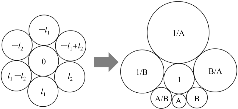
Figure 3: Left: adjacent circles in hexagonal packing, Right: the ratio of the radii of adjacent circles in the Doyle spiral

The Doyle spirals are the image of a hexagonal lattice in the complex plane ${\mathbb{C}}$ by exponential maps [5]. In [7], conformally symmetric circle packings were defined as a generalization of the Doyle spirals. In order to generate such circle packings, the determination of the radius of each circle is also necessary, which is not the scope of this article. From the aspect of the golden angle method, packings with the Voronoi cells of varying volumes have been investigated in [35], [39].

Example 3 (PDE for $n=2$).

From Proposition 2, the PDE for $n=2$ is $(\phi_{2}^{-1}(\phi_{1})_{y})_{y}+(\phi_{1}^{-1}(\phi_{2})_{x})_{x}=0$. If ($\star\star$) is also assumed, $\epsilon(x,y):=c^{-1}\phi_{2}^{2}$ must fulfill the following:

$$\epsilon_{xx}+(\epsilon^{-1})_{yy} = c^{-1}((\phi_{2}^{2})_{xx}+(\phi_{1}^{2})_{yy})=0,$$

$$A_{1}=U^{-1}U_{x} = \begin{pmatrix}0&\phi_{2}^{-1}(\phi_{1})_{y}\\ -\phi_{2}^{-1}(\phi_{1})_{y}&0\end{pmatrix}=\begin{pmatrix}0&(\epsilon^{-1})_{y}/2\\ -(\epsilon^{-1})_{y}/2&0\end{pmatrix},$$

$$A_{2}=U^{-1}U_{y} = \begin{pmatrix}0&-\phi_{1}^{-1}(\phi_{2})_{x}\\ \phi_{1}^{-1}(\phi_{2})_{x}&0\end{pmatrix}=\begin{pmatrix}0&-\epsilon_{x}/2\\ \epsilon_{x}/2&0\end{pmatrix}.$$

$U(x,y)$ is explicitly represented by using $\theta(x,y)$ with $\epsilon_{x}=2\theta_{y}$ and $(\epsilon^{-1})_{y}=-2\theta_{x}$ as follows:

$$U(x,y)=U_{0}\exp\left(\begin{pmatrix}0&-\theta\\ \theta&0\end{pmatrix}\right)=U_{0}\begin{pmatrix}\cos\theta&-\sin\theta\\ \sin\theta&\cos\theta\end{pmatrix}\quad(U_{0}\in O(2)).$$

All the solutions of inviscid Burgers equation $\epsilon\epsilon_{x}+\epsilon_{y}=0$ fulfill $\epsilon_{xx}+(\epsilon^{-1})_{yy}=0$, which is also seen from the following decomposition:

$$\epsilon_{xx}+(\epsilon^{-1})_{yy}=\left(\frac{\partial}{\partial x}-\frac{\partial}{\partial y}\epsilon^{-1}\right)\left(\frac{\partial}{\partial x}+\epsilon^{-1}\frac{\partial}{\partial y}\right)\epsilon.$$

As a result, non-trivial solutions of Eqs.(14),(15) for dimensions $n>2$ are obtained by setting $\phi_{2k-1}^{2}({\mathbf{x}})=c_{k}/\epsilon_{k}(x_{2k-1},x_{2k})$, $\phi_{2k}^{2}({\mathbf{x}})=c_{k}\epsilon_{k}(x_{2k-1},x_{2k})$, (and $\phi_{n}({\mathbf{x}})=c_{(n+1)/2}$ if $n$ is odd) for some constants $c_{k}$ and solutions of $\epsilon_{k}(\epsilon_{k})_{x}+(\epsilon_{k})_{y}=0$.

Example 4 (Case of inviscid Burgers equation $\epsilon_{xx}+(\epsilon^{-1})_{yy}=0$).

Let $\epsilon(x,y)$ be the solution of the following inviscid Burgers equation:

$$\begin{cases}\epsilon\epsilon_{x}+\epsilon_{y}=0,\\ \epsilon(t,0)=h(t)\text{ for any }t\in I,\end{cases}$$ (18)

where $h(x):I\rightarrow{\mathbb{R}}$ is the initial condition given on an interval $I\subset{\mathbb{R}}$.

The map $f(x,y)$ with the following Jacobian matrix, can be determined as follows:

$$\begin{pmatrix}(f_{1})_{x}&(f_{1})_{y}\\ (f_{2})_{x}&(f_{2})_{y}\\ \end{pmatrix}=\begin{pmatrix}\cos\theta(x,y)&-\sin\theta(x,y)\\ \sin\theta(x,y)&\cos\theta(x,y)\\ \end{pmatrix}\begin{pmatrix}\epsilon^{-1/2}&0\\ 0&\epsilon^{1/2}\\ \end{pmatrix}.$$ (19)

From $\epsilon\epsilon_{x}+\epsilon_{y}=0$,

$$2\theta_{x} = -(\epsilon^{-1})_{y}=-\epsilon^{-1}\epsilon_{x},$$

$$2\theta_{y} = \epsilon_{x}=-\epsilon^{-1}\epsilon_{y}.$$

Thus, $\theta=-(\log\epsilon+d)/2$ for some constant $d$. The inviscid Burgers equation can be solved by using the characteristic equation:

$$\begin{cases}q^{\prime}(s)=\epsilon(q(s),s),\\ q(0)=t.\end{cases}$$ (20)

From Eq.(20), $q^{\prime}(0)=\epsilon(t,0)=h(t)$. On the characteristic curve, $q^{\prime}(s)=\epsilon(q(s),s)$ is constant because

$$\frac{d}{ds}\epsilon(q(s),s)=q^{\prime}(s)\epsilon_{x}(q(s),s)+\epsilon_{y}(q(s),s)=\epsilon(q(s),s)\epsilon_{x}(q(s),s)+\epsilon_{y}(q(s),s)=0.$$

Hence, $q(s)=t+h(t)s$ ($s\in{\mathbb{R}}$) is the characteristic line, on which $f=(f_{1},f_{2})$ satisfies:

$$\frac{d}{ds}f_{1}(q(s),s) = q^{\prime}(s)(f_{1})_{x_{1}}+(f_{1})_{x_{2}}=\epsilon^{1/2}\left(\cos\frac{\log\epsilon+d}{2}+\sin\frac{\log\epsilon+d}{2}\right),$$

$$\frac{d}{dt}f_{2}(q(s),s) = q^{\prime}(s)(f_{2})_{x_{1}}+(f_{2})_{x_{2}}=\epsilon^{1/2}\left(\cos\frac{\log\epsilon+d}{2}-\sin\frac{\log\epsilon+d}{2}\right).$$

Without loss of generality, $d=-\pi/2$ may be assumed. In this case, for any $(x,y)\in{\mathbb{R}}^{2}$ and $t\in I$ that satisfies $t+h(t)y=x$, $f=(f_{1},f_{2})$ is given by

$$f(x,y) = f(t,0)+y\sqrt{2h(t)}\begin{pmatrix}\sin\frac{\log h(t)}{2}\\ \cos\frac{\log h(t)}{2}\end{pmatrix},$$

$$f(t,0) = \begin{pmatrix}\int(f_{1})_{x_{1}}(t,0)dt\\ \int(f_{2})_{x_{1}}(t,0)dt\end{pmatrix}=\begin{pmatrix}\int\frac{1}{\sqrt{h(t)}}\cos\frac{\log h(t)-\pi/2}{2}dt\\ -\int\frac{1}{\sqrt{h(t)}}\sin\frac{\log h(t)-\pi/2}{2}dt\end{pmatrix}.$$

In particular, if $f_{1}(t,0)\cos\frac{\log h(t)}{2}\neq f_{2}(t,0)\sin\frac{\log h(t)}{2}$,

$$f(x,y) = (f_{1}(t,0)\cos\frac{\log h(t)}{2}-f_{2}(t,0)\sin\frac{\log h(t)}{2})\begin{pmatrix}Y&1\\ -1&Y\\ \end{pmatrix}\begin{pmatrix}\sin\frac{\log h(t)}{2}\\ \cos\frac{\log h(t)}{2}\end{pmatrix},$$

$$Y = \frac{y\sqrt{2h(t)}+f_{1}(t,0)\sin\frac{\log h(t)}{2}+f_{2}(t,0)\cos\frac{\log h(t)}{2}}{f_{1}(t,0)\cos\frac{\log h(t)}{2}-f_{2}(t,0)\sin\frac{\log h(t)}{2}}.$$

Otherwise, by using $g(t):=f_{1}(t,0)/\sin\frac{\log h(t)}{2}=f_{2}(t,0)/\cos\frac{\log h(t)}{2}$,

$$f(x,y) = Y\begin{pmatrix}\sin\frac{\log h(t)}{2}\\ \cos\frac{\log h(t)}{2}\end{pmatrix},\quad Y=y\sqrt{2h(t)}+g(t).$$

Both correspond to the case of Eq.(3), if $f$ is regarded as the function of $(t,Y)$.

3.2 A family of solutions obtained by separation of variables

Another family of solutions of $\epsilon_{xx}+(\epsilon^{-1})_{yy}=0$ can be obtained by separation of variables. If we put $\epsilon(x,y)=F(x)/G(y)$, $F^{\prime\prime}(x)/G(y)=-G^{\prime\prime}(y)/F(x)$ is obtained from $\epsilon_{xx}=-(\epsilon^{-1})_{yy}$. Hence, for some constant $\alpha$,

$$F(x)F^{\prime\prime}(x)=\alpha,\quad G(y)G^{\prime\prime}(y)=-\alpha.$$

If $\alpha\neq 0$, $(F^{\prime}(x))^{2}=2\alpha\log F(x)+d_{1}$, $(G^{\prime}(y))^{2}=-2\alpha\log G(y)+d_{2}$. In general, $F(x)$ and $G(y)$ are functions represented by incomplete gamma functions. We will discuss only the case of $\alpha=0$ to obtain elementary solutions.

If $\alpha=0$, $F(x)=c_{1}x+d_{1}$ and $G(y)=c_{2}y+d_{2}$ are obtained. By translating the $x$ and $y$-coordinates, it may be assumed that $\epsilon(x,y)=F(x)/G(y)$ is equal to either of (a) $\epsilon=1/\beta y$, (b) $\epsilon=\beta x$, (c) $\epsilon=\beta x/y$. In case of (a)–(c), $\epsilon$ satisfies $\epsilon\epsilon_{x}+\epsilon_{y}=0$ if and only if (c) and $\beta=1$.

Without loss of generality, $\beta>0$ may be assumed. The following examples explains each case. The case (b) is omitted, because it can be obtained from (a) by exchanging $x$ and $y$, and $f_{1}$ and $f_{2}$. The Vogel spiral is a special case of (a).

Example 5 ((a) $\epsilon(x,y)=1/\beta y$: packing of a disk).

In this example, $\varphi$ is always set to $1/(1+\gamma_{1})=(3-\sqrt{5})/2$. As for the basis matrix $B$ of $L$, we will consider the following:

$$\text{(i) }\begin{pmatrix}1&-\varphi\\ 0&-1\end{pmatrix},\quad\text{(ii) }\begin{pmatrix}1&-\varphi\\ 1&-\overline{\varphi}\\ \end{pmatrix},\quad\text{(iii) }\begin{pmatrix}0&-1\\ 1&-\overline{\varphi}\\ \end{pmatrix},$$

It was proved in Theorem 1 that the lattice basis in (ii) is optimal based on the stability of the packing density.

The map $f$ is as follows, up to similarity transformations.

$$f(x,y)=\sqrt{y}\begin{pmatrix}\cos(\beta x/2)\\ \sin(\beta x/2)\end{pmatrix},$$

which is injective on the following ${\mathfrak{D}}$:

$${\mathfrak{D}}:=\left\{(x,y)\in{\mathbb{R}}^{2}:0\leq x<4\pi/\beta,\ 0<y<M\right\}.$$

In order to smoothly connect the spiral patterns near the half-lines $x=0$ and $x=4\pi/\beta$, the mapped lattice $L$ needs to contain a vector very close to ${\hskip 1.42262pt{}^{t}(4\pi/\beta,0)}$.

1. If $s:=4\pi/\beta$ is an integer, then ${\hskip 1.42262pt{}^{t}(s,0)}$ is precisely contained in $L(B)$. If $s=1$, $f(L(B)\cap{\mathfrak{D}})$ is the same as the Vogel spiral.

   $$f(L(B)\cap{\mathfrak{D}}):=\left\{\sqrt{n}(\cos(2\pi n\varphi/s),\sin(2\pi n\varphi/s)):n\in{\mathbb{Z}},\ 0<n<M\right\}.$$

   As shown in (i) of Figure 4, the points $f(L(B)\cap{\mathfrak{D}})$ are rather sparse around the origin for large $s$, because $\epsilon=s/4\pi y$ is not sufficiently small (cf. (2) of Theorem 1). The sparsity can be avoided by using the basis (ii) instead.

2. In this case, $L(B)$ does not contain any vectors of the form ${\hskip 1.42262pt{}^{t}(s,0)}$. However, the $n$’th convergent $p_{n}^{(-)}/q_{n}^{(-)}$ of $-1/\overline{\varphi}$ fulfills:

   $$\begin{pmatrix}1&-\varphi\\ 1&-\overline{\varphi}\end{pmatrix}\begin{pmatrix}q_{n}^{(-)}\\ -p_{n}^{(-)}\end{pmatrix} = \begin{pmatrix}q_{n}^{(-)}+p_{n}^{(-)}\varphi\\ q_{n}^{(-)}+p_{n}^{(-)}\overline{\varphi}\\ \end{pmatrix}$$

   $$= \begin{pmatrix}2q_{n}^{(-)}+p_{n}^{(-)}(\varphi+\overline{\varphi})\\ 0\end{pmatrix}+q_{n}^{(-)}\overline{\varphi}\left(-\overline{\varphi}^{-1}-\frac{p_{n}^{(-)}}{q_{n}^{(-)}}\right)\begin{pmatrix}1\\ -1\end{pmatrix}.$$

   Therefore, by setting $s$ to one of ${\left\lvert 2q_{n}^{(-)}+p_{n}^{(-)}(\varphi+\overline{\varphi})\right\rvert}$ ($n\geq 0$), it is possible to glue the spiral patterns near the boundary of ${\mathfrak{D}}$ apparently smoothly, as seen in (ii) of Figure 4. This technique of setting $s$ to a special value will be also used in the other examples.

3. As in case (ii), although $L(B)$ does not contain any vectors ${\hskip 1.42262pt{}^{t}(s,0)}$, the boundary problem can be avoided, by putting $s={\left\lvert p_{n}^{(-)}\right\rvert}$, because

   $$\begin{pmatrix}0&-1\\ 1&-\overline{\varphi}\end{pmatrix}\begin{pmatrix}q_{n}^{(-)}\\ -p_{n}^{(-)}\end{pmatrix} = \begin{pmatrix}p_{n}^{(-)}\\ q_{n}^{(-)}+p_{n}^{(-)}\overline{\varphi}\\ \end{pmatrix}\approx\begin{pmatrix}p_{n}^{(-)}\\ 0\end{pmatrix}.$$

   The packing becomes sparse at the coordinates farther from the origin, as seen in (iii) of Figure 4. The number of spines is equal to the parameter $s={\left\lvert p_{n}^{(-)}\right\rvert}$.

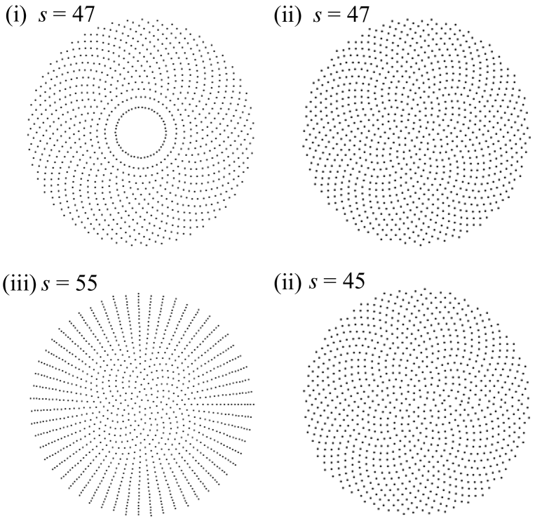
Figure 4: Packings in a disk obtained from the lattice bases (i)–(iii) of Example 5. The parameter $s$ is set to (i), (ii) $s=2q_{9}^{(-)}+(\gamma_{1}+\overline{\gamma}_{1})p_{9}^{(-)}=47$, where $p_{9}^{(-)}=-21$, $q_{9}^{(-)}=55$ are the ninth convergent of $-1/\overline{\varphi}=(-3+\sqrt{5})/2$, and (iii) $s=-p_{11}^{(-)}=55$. As for (ii), the case of $s=45\neq 2q_{n}^{(-)}+(\gamma_{1}+\overline{\gamma}_{1})p_{n}^{(-)}$ ($n\in{\mathbb{Z}}_{>0}$) is also presented as the case in which the spirals are not smoothly connected around the $x>0$ part of the $x$-axis.

It is known that the parastichies in the Vogel spiral are the Fermat spiral. In fact, the image of $(x,y)$ by the following $f$ has the polar coordinate $(r,\theta)=(\sqrt{y},\beta x/2)$.

$$f(x,y)=\sqrt{y}\begin{pmatrix}\cos(\beta x/2)\\ \sin(\beta x/2)\end{pmatrix}.$$

If $x,y$ is colinear, $(r,\theta)=(\sqrt{y},\beta x/2)$ satisfies a linear equation $r^{2}=a+b\theta$ for some constants $a$ and $b$, which is an equation of the Fermat spiral. In the case of (c), the image of any line $y=ax$ passing through the origin by the map $f$ in Eq.(21), is a logarithmic spiral, because $\log r$ and $\theta$ fulfill a linear equation.

Example 6 ((c) $\epsilon(x,y)=\beta x/y$, case of logarithmic spirals).

The map $f$ is as follows, up to similarity transformations:

$$f(x,y)=\sqrt{xy}\begin{pmatrix}\cos\theta(x,y)\\ \sin\theta(x,y)\\ \end{pmatrix},\quad\theta(x,y)=-\displaystyle\frac{\beta^{-1}}{2}\log{\left\lvert x\right\rvert}+\frac{\beta}{2}\log{\left\lvert y\right\rvert}.$$ (21)

The map $f$ is injective on the ${\mathfrak{D}}$:

$${\mathfrak{D}}:=\left\{(x,y)\in{\mathbb{R}}^{2}:0<\log x\leq\frac{4\pi}{\beta+\beta^{-1}},\ 0<y\leq M\right\}.$$

As in the previous example, it is necessary to set $s:=\exp(4\pi/(\beta+\beta^{-1}))$ to a positive integer $s=q_{n}^{(-)}+(\gamma_{1}+\overline{\gamma}_{1})p_{n}^{(-)}$. Since $X^{2}-(4\pi/\log s)X+1=0$ has a real root $\beta$, $1\leq s<e^{2\pi}\approx 535.5$ is also required.

Proposition 3 is a case of dimension $n=3$.

Proposition 3.

If $n=3$ and $A_{3}=0$, the solutions $\phi_{1}({\mathbf{x}}),\phi_{2}({\mathbf{x}}),\phi_{3}({\mathbf{x}})$ for the system of PDEs in Eqs.(14), (15) are as follows, for some constants $d,d_{2}$ and $\epsilon(x_{1},x_{2})$ with $\epsilon_{x_{1}x_{1}}+(\epsilon^{-1})_{x_{2}x_{2}}=-2d_{2}^{2}$:

$$\phi_{1}({\mathbf{x}}) = c^{1/3}(d^{3}+3d_{2}x_{3})^{1/3}\epsilon^{-1/2}(x_{1},x_{2}),$$

$$\phi_{2}({\mathbf{x}}) = c^{1/3}(d^{3}+3d_{2}x_{3})^{1/3}\epsilon^{1/2}(x_{1},x_{2}),$$

$$\phi_{3}({\mathbf{x}}) = c^{1/3}(d^{3}+3d_{2}x_{3})^{-2/3}.$$

Proof.

From $A_{3}=U^{-1}U_{x_{3}}=O$, $U$ is independent of $x_{3}$. From (16), $(\phi_{3})_{x_{1}}=(\phi_{3})_{x_{2}}=0$ also holds. From Eq.(15), $\left(\phi_{3}^{-1}(\phi_{1})_{x_{3}}\right)_{x_{3}}=\left(\phi_{3}^{-1}(\phi_{2})_{x_{3}}\right)_{x_{3}}=0$. Thus, if we put $G(x_{3}):=\int_{0}^{x_{3}}\phi_{3}(x_{1},x_{2},x)dx$, the following holds for some $F_{i}(x_{1},x_{2})$ and $H_{i}(x_{1},x_{2})$.

$$\phi_{i}({\mathbf{x}})=F_{i}(x_{1},x_{2})G(x_{3})+H_{i}(x_{1},x_{2})\quad(i=1,2).$$

From $\phi_{1}\phi_{2}\phi_{3}=c$, $(\phi_{1}\phi_{2})_{x_{j}}=0$ holds for $j=1,2$. Therefore, for some $\alpha_{1},\alpha_{2},\beta_{1},\beta_{2}\in{\mathbb{R}}$ and $\tilde{F}(x_{1},x_{2})$,

$$\phi_{1}({\mathbf{x}}) = (\alpha_{1}G(x_{3})+\beta_{1})\tilde{F}(x_{1},x_{2}),$$

$$\phi_{2}({\mathbf{x}}) = (\alpha_{2}G(x_{3})+\beta_{2})/\tilde{F}(x_{1},x_{2}).$$

From Eq.(14) and Eq.(15),

$$(\phi_{1})_{x_{2}x_{3}} = \phi_{2}^{-1}(\phi_{2})_{x_{3}}(\phi_{1})_{x_{2}},$$ (22)

$$(\phi_{2})_{x_{1}x_{3}} = \phi_{1}^{-1}(\phi_{1})_{x_{3}}(\phi_{2})_{x_{1}},$$ (23)

$$\left(\phi_{1}^{-1}(\phi_{2})_{x_{1}}\right)_{x_{1}}+\left(\phi_{2}^{-1}(\phi_{1})_{x_{2}}\right)_{x_{2}} = -\phi_{3}^{-2}(\phi_{1})_{x_{3}}(\phi_{2})_{x_{3}}.$$ (24)

From the first two equalities, $\left(\log(\phi_{1})_{x_{2}}\right)_{x_{3}}=(\log\phi_{2})_{x_{3}}$, $\left(\log(\phi_{2})_{x_{1}}\right)_{x_{3}}=(\log\phi_{1})_{x_{3}}$. Thus, the following functions are independent of $x_{3}$.

$$\phi_{2}^{-1}(\phi_{1})_{x_{2}}=\displaystyle\frac{1}{2}\frac{\alpha_{1}G(x_{3})+\beta_{1}}{\alpha_{2}G(x_{3})+\beta_{2}}(\tilde{F}^{2})_{x_{2}},\quad\phi_{1}^{-1}(\phi_{2})_{x_{1}}=\displaystyle\frac{1}{2}\frac{\alpha_{2}G(x_{3})+\beta_{2}}{\alpha_{1}G(x_{3})+\beta_{1}}(\tilde{F}^{-2})_{x_{1}}.$$

Hence, it is possible to choose $r_{1},r_{2}\neq 0$, $d,d_{2}\in{\mathbb{R}}$ and $\tilde{F}(x,y)$ so that $\phi_{1}=r_{1}(d+d_{2}G(x_{3}))\tilde{F}(x_{1},x_{2})$ and $\phi_{2}=r_{2}(d+d_{2}G(x_{3}))/\tilde{F}(x_{1},x_{2})$. Thus, the following are obtained from $\phi_{1}\phi_{2}\phi_{3}=r_{1}r_{2}(d+d_{2}G(x_{3}))^{2}\phi_{3}(x_{3})=c$, $\phi_{3}(x_{3})=G^{\prime}(x_{3})$, $G(0)=0$ and Eq.(24):

$$r_{1}r_{2}(d+d_{2}G(x_{3}))^{3} = r_{1}r_{2}d^{3}+3cd_{2}x_{3},$$

$$\frac{r_{2}}{2r_{1}}(\tilde{F}^{-2})_{x_{1}x_{1}}+\frac{r_{1}}{2r_{2}}(\tilde{F}^{2})_{x_{2}x_{2}} = -r_{1}r_{2}d_{2}^{2}.$$

If we put $\epsilon(x_{1},x_{2}):=(r_{2}/r_{1})\tilde{F}(x_{1},x_{2})^{-2}$, $\epsilon_{x_{1}x_{1}}+(\epsilon^{-1})_{x_{2}x_{2}}=-2(r_{1}r_{2})d_{2}^{2}$ is obtained, in addition to the following.

$$\phi_{1}({\mathbf{x}}) = (r_{1}r_{2})^{1/2}(d^{3}+3(cd_{2}/r_{1}r_{2})x_{3})^{1/3}\epsilon^{-1/2}(x_{1},x_{2}),$$

$$\phi_{2}({\mathbf{x}}) = (r_{1}r_{2})^{1/2}(d^{3}+3(cd_{2}/r_{1}r_{2})x_{3})^{1/3}\epsilon^{1/2}(x_{1},x_{2}),$$

$$\phi_{3}({\mathbf{x}}) = c(r_{1}r_{2})^{-1}(d^{3}+3(cd_{2}/r_{1}r_{2})x_{3})^{-2/3}.$$

The statement is proved if $d,d_{2}$ are replaced by $c^{1/3}(r_{1}r_{2})^{-1/2}d$, $(r_{1}r_{2})^{-1/2}d_{2}$. ∎∎

Separation of variables can also be used to obtain a family of solutions of $\epsilon_{x_{1}x_{1}}+(\epsilon^{-1})_{x_{2}x_{2}}=-2d_{2}^{2}$ for $d_{2}\neq 0$. A packing of a ball (i.e., 3D analogue of the Vogel spiral), is obtained as a result; if we put $\epsilon(x_{1},x_{2})=F(x_{1})/G(x_{2})$, $\epsilon_{x_{1}x_{1}}+(\epsilon^{-1})_{x_{2}x_{2}}+2d_{2}^{2}=0$ implies:

$$F(x_{1})F^{\prime\prime}(x_{1})+G(x_{2})G^{\prime\prime}(x_{2})+2d_{2}^{2}F(x_{1})G(x_{2})=0.$$

Hence, $F(x_{1})$ or $G(x_{2})$ must be a constant function, and either of (a) $\epsilon=d_{0}+d_{1}x_{1}-(d_{2}x_{1})^{2}$ or (b) $\epsilon=1/\{d_{0}+d_{1}x_{2}-(d_{2}x_{2})^{2}\}$ holds. The part (b) can be obtained by swapping the roles of $x_{1}$ and $x_{2}$, and $f_{1}$ and $f_{2}$ in (a). Therefore, we will discuss only the case (a).

Example 7 (Packing of a ball, 3D Vogel spiral).

From $\epsilon=d_{0}+d_{1}x_{1}-(d_{2}x_{1})^{2}$, $d_{2}\neq 0$ and $A_{k}={\hskip 1.42262pt{}^{t}{\mathbf{e}}_{k}}{\mathbf{c}}_{k}-{\hskip 1.42262pt{}^{t}{\mathbf{c}}_{k}}{\mathbf{e}}_{k}$,

$$A_{1}=\begin{pmatrix}0&0&d_{2}\epsilon^{-1/2}\\ 0&0&0\\ -d_{2}\epsilon^{-1/2}&0&0\\ \end{pmatrix},\quad A_{2}=\begin{pmatrix}0&-\epsilon_{x_{1}}/2&0\\ \epsilon_{x_{1}}/2&0&d_{2}\epsilon^{1/2}\\ 0&-d_{2}\epsilon^{1/2}&0\\ \end{pmatrix},\quad A_{3}=O.$$

The following $D_{j},V_{j}$ ($j=1,2$) provide diagonalizations $A_{1}=V_{1}D_{1}V_{1}^{*}$, $A_{2}=V_{2}D_{2}V_{2}^{*}$ of $A_{1}$ and $A_{2}$.

$$D_{1} = d_{2}\epsilon^{-1/2}\begin{pmatrix}i&0&0\\ 0&-i&0\\ 0&0&0\end{pmatrix},\quad V_{1}=\frac{1}{\sqrt{2}}\begin{pmatrix}-i&i&0\\ 0&0&\sqrt{2}\\ 1&1&0\\ \end{pmatrix},$$

$$D_{2} = \sqrt{d_{1}^{2}/4+d_{0}d_{2}^{2}}\begin{pmatrix}i&0&0\\ 0&-i&0\\ 0&0&0\end{pmatrix},$$

$$V_{2} = \frac{1}{\sqrt{2(d_{1}^{2}/4+d_{0}d_{2}^{2})}}\begin{pmatrix}\epsilon_{x_{1}}/2&\epsilon_{x_{1}}/2&-\sqrt{2}d_{2}\epsilon^{1/2}\\ -i\sqrt{d_{1}^{2}/4+d_{0}d_{2}^{2}}&i\sqrt{d_{1}^{2}/4+d_{0}d_{2}^{2}}&0\\ d_{2}\epsilon^{1/2}&d_{2}\epsilon^{1/2}&\sqrt{2}\epsilon_{x_{1}}/2\\ \end{pmatrix}.$$

From $(V_{j})_{x_{j}}=O$ and $U_{x_{j}}=UA_{j}$ ($j=1,2$), $U({\mathbf{x}})$ satisfies $(UV_{j})_{x_{j}}=UV_{j}D_{j}$. Hence, for some $U_{0}\in O(3)$,

$$U({\mathbf{x}}) \propto U_{0}\begin{pmatrix}1&0&0\\ 0&\cos\sqrt{d_{1}^{2}/4+d_{0}d_{2}^{2}}x_{2}&\sin\sqrt{d_{1}^{2}/4+d_{0}d_{2}^{2}}x_{2}\\ 0&-\sin\sqrt{d_{1}^{2}/4+d_{0}d_{2}^{2}}x_{2}&\cos\sqrt{d_{1}^{2}/4+d_{0}d_{2}^{2}}x_{2}\\ \end{pmatrix}\begin{pmatrix}d_{2}\epsilon^{1/2}&0&-\epsilon_{x_{1}}/2\\ 0&\sqrt{d_{1}^{2}/4+d_{0}d_{2}^{2}}&0\\ \epsilon_{x_{1}}/2&0&d_{2}\epsilon^{1/2}\\ \end{pmatrix}.$$

The Jacobian matrix of the map $f$ is provided as $U({\mathbf{x}})\Phi({\mathbf{x}})$. Hence, for some ${\mathbf{v}}_{0}\in{\mathbb{R}}^{3}$,

$$f({\mathbf{x}}) \propto c^{1/3}(d^{3}+3d_{2}x_{3})^{1/3}U_{0}\begin{pmatrix}-\epsilon_{x_{1}}/2d_{2}\\ \epsilon^{1/2}\sin\sqrt{d_{1}^{2}/4+d_{0}d_{2}^{2}}x_{2}\\ \epsilon^{1/2}\cos\sqrt{d_{1}^{2}/4+d_{0}d_{2}^{2}}x_{2}\\ \end{pmatrix}+\frac{c^{1/3}}{d_{2}}{\mathbf{v}}_{0}$$

$$\propto (d^{3}+3d_{2}x_{3})^{1/3}U_{0}\begin{pmatrix}d_{2}^{2}x_{1}-d_{1}/2\\ \sqrt{d_{1}^{2}/4+d_{0}d_{2}^{2}-(d_{2}^{2}x_{1}-d_{1}/2)^{2}}\sin\sqrt{d_{1}^{2}/4+d_{0}d_{2}^{2}}x_{2}\\ \sqrt{d_{1}^{2}/4+d_{0}d_{2}^{2}-(d_{2}^{2}x_{1}-d_{1}/2)^{2}}\cos\sqrt{d_{1}^{2}/4+d_{0}d_{2}^{2}}x_{2}\\ \end{pmatrix}+{\mathbf{v}}_{0}.$$

By putting $s:=1/\sqrt{d_{1}^{2}/4+d_{0}d_{2}^{2}}$, $U_{0}=I$ and ${\mathbf{v}}_{0}=0$, and replacing $x_{1}$, $x_{2}$, $x_{3}$ by $(x_{2}/rs+d_{1}/2)/d_{2}^{2}$, $2\pi x_{1}$, $(x_{3}-d^{3})/3d_{2}$ respectively, the following is obtained.

$$f({\mathbf{x}}) \propto x_{3}^{1/3}\begin{pmatrix}x_{2}\\ \sqrt{r^{2}-x_{2}^{2}}\sin(2\pi x_{1}/s)\\ \sqrt{r^{2}-x_{2}^{2}}\cos(2\pi x_{1}/s)\\ \end{pmatrix},\quad r,s>0:\text{constants.}$$

The above $f$ is injective on the ${\mathfrak{D}}$, and maps ${\mathfrak{D}}$ onto a ball of radius $R$:

$${\mathfrak{D}}:=\{(x_{1},x_{2},x_{3})\in{\mathbb{R}}^{3}:0\leq x_{1}<s,\ -r<x_{2}<r,\ 0<x_{3}<R\}.$$

As the lattice basis, $B_{3}$ of Theorem 1 can be used. Figures 6 and 7 present the surface pattern and the cross-sections of the 3D Vogel spiral for the parameters $s=1$ and $r=R=1000$.

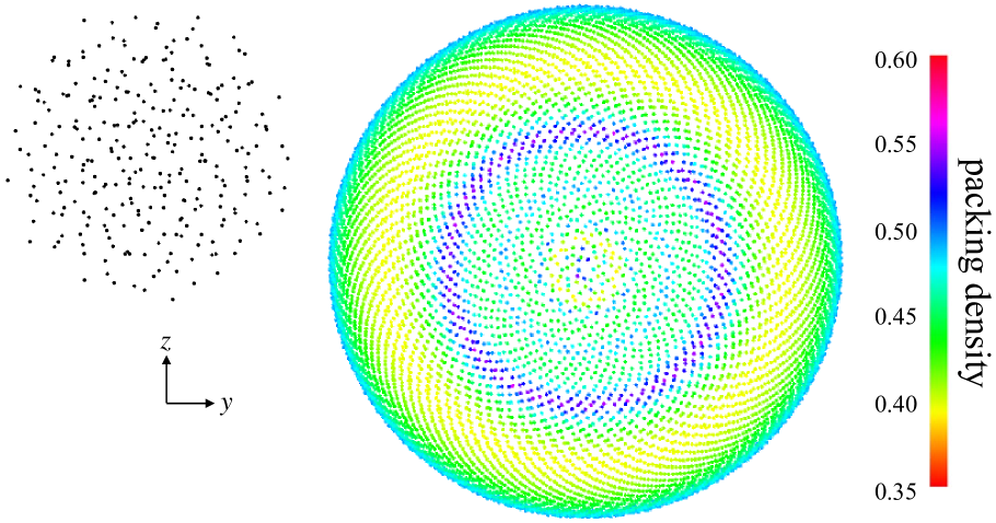
Figure 6: Point distribution around the origin (left) and the pattern on the semisphere (right) of the 3D Vogel spiral for the parameters $s=1$, $r=R=1000$.

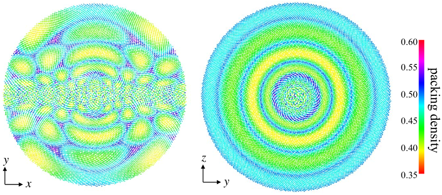
Figure 7: Cross-sections of the 3D Vogel spiral in the $x$-$y$ and $y$-$z$ planes in case of $s=1$ and $r=R=1000$.

4 General case: packing of Riemannian manifolds

Let $N\geq n>0$ be integers, and $f({\mathbf{x}})=(f_{1}({\mathbf{x}}),\dots,f_{n}({\mathbf{x}})):{\mathfrak{D}}\rightarrow{\mathbb{R}}^{N}$ be a function defined on an open subset ${\mathfrak{D}}\subset{\mathbb{R}}^{m}$ that fulfills ($\star$), ($\star\star$). Hence,

$$Df({\mathbf{x}})=U({\mathbf{x}})\begin{pmatrix}\Phi({\mathbf{x}})\\ O\end{pmatrix},\quad O:\text{$(N-n)\times n$ zero matrix.}$$

As in the previous section, if $n$ and $N$ are fixed, it is possible to derive the system of PDEs for the entries of $\Phi({\mathbf{x}})$ and $U({\mathbf{x}})$. As a fundamental question, it is also important to determine which Riemannian manifolds can be packed by the new method. Theorem 2 deals with this problem in a local sense in the case of real analytic surfaces (class $C^{\omega}$). We leave this problem in a global sense to future study. Even if the packed domain is bounded, it is possible to generate aperiodic packings consisting of arbitrarily large number of points, by setting the scale $c\rightarrow 0$ of the mapped lattice $cL$.

If the dimension $N$ is appropriately chosen, any $C^{k}$ Riemannian $n$-manifolds $(M,g)$ can be isometrically embedded into the Euclidean space ${\mathbb{R}}^{N}$ by an injective map of class $C^{k}$ ($3\leq k\leq\infty$ or $\omega$) [27], [28]. We fix an atlas $\{(U_{\alpha},\varphi_{\alpha})\}_{\alpha\in I}$ of $M$ and isometries $\iota_{\alpha}:U_{\alpha}\rightarrow\iota_{\alpha}(U_{\alpha})\subset{\mathbb{R}}^{N}$. Let $Df_{\alpha}({\mathbf{x}})$ be the Jacobian matrix of $f_{\alpha}:=\iota_{\alpha}\circ\varphi_{\alpha}^{-1}$.

For another diffeomorphism $\psi_{\alpha}:U_{\alpha}\to\psi_{\alpha}(U_{\alpha})\subset{\mathbb{R}}^{n}$ and any open subset $V\subset\psi_{\alpha}(U_{\alpha})$, it is straightforward to see that the Jacobian matrix of $\iota_{\alpha}\circ\psi_{\alpha}^{-1}$ fulfills ($\star$) and ($\star\star$) on $V$ if and only if the following ($\flat$) holds:

• The diffeomorphism ${\mathbf{x}}=\sigma({\mathbf{y}}):=\varphi_{\alpha}\circ\psi_{\alpha}^{-1}$ on $V$ has the Jacobian matrix $D\sigma$ such that ${\hskip 1.42262pt{}^{t}(D\sigma({\mathbf{y}}))}{\hskip 1.42262pt{}^{t}(Df_{\alpha}(\sigma({\mathbf{y}})))}Df_{\alpha}(\sigma({\mathbf{y}}))D\sigma({\mathbf{y}})$ is diagonal, and has a constant determinant.

In particular, if $\varphi_{\alpha}$ is an isothermal coordinate system, i.e., ${\hskip 1.42262pt{}^{t}(Df_{\alpha}({\mathbf{x}}))}Df_{\alpha}({\mathbf{x}})=\lambda({\mathbf{x}})I$ for some positive-valued function $\lambda({\mathbf{x}})$, then ($\flat$) occurs if and only if ${\hskip 1.42262pt{}^{t}(D\sigma({\mathbf{y}}))}D\sigma({\mathbf{y}})$ is diagonal, and

$$\det({\hskip 1.42262pt{}^{t}(D\sigma({\mathbf{y}}))}D\sigma({\mathbf{y}}))=c^{2}\lambda^{-2}(\sigma({\mathbf{y}})).$$

In Theorem 2, we assume that $n=2$, and the Riemannian surface $(M,g)$ is real analytic in order to use the Cauchy-Kovalevskaya theorem.

Theorem 2.

For any constant $c\neq 0$ and real analytic Riemannian surface $(M,g)$, there is an atlas $\{(U_{\alpha},\varphi_{\alpha})\}_{\alpha\in I}$ of $M$ such that for any $\alpha\in I$, we have a real analytic function $\epsilon(x_{1},x_{2})$ on $\varphi_{\alpha}(U_{\alpha})$ with

$$g|_{U_{\alpha}}=\frac{c^{2}}{\epsilon(x_{1},x_{2})}dx_{1}^{2}+\epsilon(x_{1},x_{2})dx_{2}^{2}.$$

Thus, for any isometry $\iota_{\alpha}:U_{\alpha}\rightarrow\iota_{\alpha}(U_{\alpha})\subset{\mathbb{R}}_{N}$, $\iota_{\alpha}\circ\varphi_{\alpha}^{-1}$ fulfills ($\star$), ($\star\star$).

Proof.

For any $p\in M$, fix a neighborhood $p\in U_{\alpha}\subset M$, a diffeomorphism $\varphi_{\alpha}:U_{\alpha}\rightarrow\varphi_{\alpha}(U_{\alpha})\subset{\mathbb{R}}^{2}$ and an isometry $\iota_{\alpha}:U_{\alpha}\rightarrow\iota_{\alpha}(U_{\alpha})\subset{\mathbb{R}}^{2}$. We may assume that $\varphi_{\alpha}$ is an isothermal coordinate system. We shall prove that for $f_{\alpha}:=\iota_{\alpha}\circ\varphi_{\alpha}^{-1}$, some neighborhood $V\subset U_{\alpha}$ of $p$ and diffeomorphism $\sigma$ with the inverse $\sigma^{-1}:\varphi_{\alpha}(V)\rightarrow{\mathbb{R}}^{2}$ (hence, $\psi_{\alpha}:=\sigma^{-1}\circ\varphi_{\alpha}|_{V}$) satisfy ($\flat$). If so, the chart $(V,\psi_{\alpha})$ has the desired property.

$D\sigma^{-1}({\mathbf{x}}){\hskip 1.42262pt{}^{t}(D\sigma^{-1}({\mathbf{x}}))}=({\hskip 1.42262pt{}^{t}(D\sigma(\sigma^{-1}({\mathbf{x}})))}D\sigma(\sigma^{-1}({\mathbf{x}})))^{-1}$ is diagonal and the determinant of $D\sigma^{-1}({\mathbf{x}}){\hskip 1.42262pt{}^{t}(D\sigma^{-1}({\mathbf{x}}))}$ is equal to $c^{-2}\lambda^{2}({\mathbf{x}})$, if and only if $D\sigma^{-1}$ is represented as follows:

$$D\sigma^{-1}(x_{1},x_{2}) = c^{-1}\lambda(x_{1},x_{2})\begin{pmatrix}\epsilon^{1/2}(x_{1},x_{2})&0\\ 0&\pm\epsilon^{-1/2}(x_{1},x_{2})\end{pmatrix}U(x_{1},x_{2}),$$

$$U(x_{1},x_{2}) = \begin{pmatrix}\cos\theta(x_{1},x_{2})&\sin\theta(x_{1},x_{2})\\ -\sin\theta(x_{1},x_{2})&\cos\theta(x_{1},x_{2})\end{pmatrix}.$$

If we put $B_{i}:=(D\sigma^{-1})^{-1}(D\sigma^{-1})_{x_{i}}$ and $A_{i}:=U^{-1}U_{x_{i}}$,

$$B_{i} = \frac{\lambda_{x_{i}}}{\lambda}I+\frac{\epsilon_{x_{i}}}{2\epsilon}{\hskip 1.42262pt{}^{t}U}\begin{pmatrix}1&0\\ 0&-1\end{pmatrix}U+A_{i}$$

$$= \frac{\lambda_{x_{i}}}{\lambda}I+\frac{\epsilon_{x_{i}}}{2\epsilon}\begin{pmatrix}\cos 2\theta(x_{1},x_{2})&\sin 2\theta(x_{1},x_{2})\\ \sin 2\theta(x_{1},x_{2})&-\cos 2\theta(x_{1},x_{2})\end{pmatrix}+\theta_{x_{i}}\begin{pmatrix}0&1\\ -1&0\end{pmatrix}.$$

From the symmetry of second derivatives, the second column of $(D\sigma^{-1})B_{1}$ and the first column of $(D\sigma^{-1})B_{2}$ must be equal. Hence, the second column of $B_{1}$ and the first column of $B_{2}$ are also equal:

$$\frac{\lambda_{x_{1}}}{\lambda}\begin{pmatrix}0\\ 1\end{pmatrix}+\frac{\epsilon_{x_{1}}}{2\epsilon}\begin{pmatrix}\sin 2\theta(x_{1},x_{2})\\ -\cos 2\theta(x_{1},x_{2})\end{pmatrix}+\theta_{x_{1}}\begin{pmatrix}1\\ 0\end{pmatrix}=\frac{\lambda_{x_{2}}}{\lambda}\begin{pmatrix}1\\ 0\end{pmatrix}+\frac{\epsilon_{x_{2}}}{2\epsilon}\begin{pmatrix}\cos 2\theta(x_{1},x_{2})\\ \sin 2\theta(x_{1},x_{2})\end{pmatrix}+\theta_{x_{2}}\begin{pmatrix}0\\ -1\end{pmatrix}.$$

Thus,

$$\begin{pmatrix}\cos 2\theta(x_{1},x_{2})&-\sin 2\theta(x_{1},x_{2})\\ \sin 2\theta(x_{1},x_{2})&\cos 2\theta(x_{1},x_{2})\end{pmatrix}\begin{pmatrix}(\log\epsilon)_{x_{2}}\\ (\log\epsilon)_{x_{1}}\end{pmatrix}=2\begin{pmatrix}-(\log\lambda)_{x_{2}}+\theta_{x_{1}}\\ (\log\lambda)_{x_{1}}+\theta_{x_{2}}\end{pmatrix}.$$

From $((\log\epsilon)_{x_{2}})_{x_{1}}=((\log\epsilon)_{x_{1}})_{x_{2}}$,

$$\begin{pmatrix}1&\tan 2\theta\\ \end{pmatrix}\left(\begin{pmatrix}-(\log\lambda)_{x_{1}x_{2}}+2\theta_{x_{1}x_{1}}\\ (\log\lambda)_{x_{1}x_{1}}+2\theta_{x_{1}x_{2}}\end{pmatrix}+2\theta_{x_{2}}\begin{pmatrix}-(\log\lambda)_{x_{2}}+2\theta_{x_{1}}\\ (\log\lambda)_{x_{1}}+2\theta_{x_{2}}\end{pmatrix}\right)$$

$$= \begin{pmatrix}-\tan 2\theta&1\end{pmatrix}\left(\begin{pmatrix}-(\log\lambda)_{x_{2}x_{2}}+2\theta_{x_{1}x_{2}}\\ (\log\lambda)_{x_{1}x_{2}}+2\theta_{x_{2}x_{2}}\end{pmatrix}-2\theta_{x_{1}}\begin{pmatrix}-(\log\lambda)_{x_{2}}+2\theta_{x_{1}}\\ (\log\lambda)_{x_{1}}+2\theta_{x_{2}}\end{pmatrix}\right).$$

From the Cauchy-Kovalevskaya theorem, Eq.(4) has a real analytic solution $\theta$ defined on $\varphi_{\alpha}(V)$ for a simply-connected neighborhood $p\in V\subset U$. From this $\theta$, $\log\epsilon$ and $\sigma^{-1}(x_{1},x_{2})$ can be constructed by solving the PDEs. ∎∎

Next, we prove Theorem 3. For any diffeomorphism $\sigma:U\rightarrow V$ between open subsets of two manifolds and metric $g$ on $V$, For any $p\in U$ and $u,v\in T_{p}U$, the pullback metric $\sigma^{*}g$ is defined by

$$(\sigma^{*}g)_{p}(u,v)=g_{\sigma(p)}(d\sigma_{p}(u),d\sigma_{p}(v)).$$

Theorem 3.

For any integers $0<n<N$, and $2\leq k\leq\infty$ or $k=\omega$, let $f({\mathbf{x}})\in C^{k}({\mathfrak{D}},{\mathbb{R}}^{N})$ be a function on a simply-connected open subset ${\mathfrak{D}}\subset{\mathbb{R}}^{n}$ with the Jacobian matrix $J_{f}({\mathbf{x}})$. Suppose that $f({\mathbf{x}})$ satisfies (i) and (ii) for some constant $\alpha\in{\mathbb{R}}$ and antisymmetric matrix $A$ of degree $N$:

1. ${\hskip 1.42262pt{}^{t}J_{f}({\mathbf{x}})}Q({\mathbf{x}})J_{f}({\mathbf{x}})=O$ for any ${\mathbf{x}}\in{\mathfrak{D}}$, if we put:

   $$f^{*}({\mathbf{x}}) := (\alpha I+A)f({\mathbf{x}}),$$

   $$Q({\mathbf{x}}) := f^{*}({\mathbf{x}}){\hskip 1.42262pt{}^{t}f^{*}({\mathbf{x}})}A+Af^{*}({\mathbf{x}}){\hskip 1.42262pt{}^{t}f^{*}({\mathbf{x}})}-(f^{*}({\mathbf{x}})\cdot f^{*}({\mathbf{x}}))A.$$

2. $\det({\hskip 1.42262pt{}^{t}J_{f}}({\mathbf{x}})J_{f}({\mathbf{x}}))\neq 0$, and $f^{*}({\mathbf{x}})$ is linearly independent of $f_{x_{1}}({\mathbf{x}}),\ldots,f_{x_{n}}({\mathbf{x}})$ over ${\mathbb{R}}$ for any ${\mathbf{x}}\in{\mathfrak{D}}$.

Let $H_{f}({\mathbf{x}})$ be the function on ${\mathfrak{D}}$ determined by the following equations, except for the constant term:

$$(H_{f})_{x_{j}}({\mathbf{x}}) = \frac{f^{*}({\mathbf{x}})\cdot f_{x_{j}}({\mathbf{x}})}{f^{*}({\mathbf{x}})\cdot f^{*}({\mathbf{x}})}\quad(j=1,\ldots,n).$$

Let $q_{f}=(q_{ij})_{1\leq i,j\leq n}$ be the positive-definite symmetric matrix.

$$q_{f}({\mathbf{x}}) := e^{-\frac{2(n+1)}{n}\alpha H_{f}({\mathbf{x}})}\left(f^{*}({\mathbf{x}})\cdot f^{*}({\mathbf{x}})\right)^{\frac{1}{n}}{\hskip 1.42262pt{}^{t}J_{f}}({\mathbf{x}})\left(I-\frac{f^{*}({\mathbf{x}}){\hskip 1.42262pt{}^{t}f^{*}({\mathbf{x}})}}{{\hskip 1.42262pt{}^{t}f^{*}({\mathbf{x}})}f^{*}({\mathbf{x}})}\right)J_{f}({\mathbf{x}}).$$

Hence, $g_{f}=\sum_{i,j=1}^{n}q_{ij}dx_{i}dx_{j}$ is a Riemannian metric on ${\mathfrak{D}}$. For any function $h({\mathbf{x}},x_{n+1})$ on ${\mathfrak{D}}\times{\mathbb{R}}_{>0}$, $F_{f,h}({\mathbf{x}},x_{n+1}):{\mathfrak{D}}\times{\mathbb{R}}_{>0}\rightarrow{\mathbb{R}}^{N}$ is defined by

$$F_{f,h}({\mathbf{x}},x_{n+1}) := e^{\alpha h({\mathbf{x}},x_{n+1})}\exp(Ah({\mathbf{x}},x_{n+1}))f({\mathbf{x}}).$$ (26)

The following (a) and (b) are equivalent:

1. $F_{f,h}({\mathbf{x}},x_{n+1})$ satisfies ($\star$), ($\star\star$) for some $h({\mathbf{x}},x_{n+1})\in C^{k}({\mathfrak{D}}\times{\mathbb{R}}_{>0},{\mathbb{R}})$.

2. The metric $g_{f}$ is diagonal and has a constant determinant on ${\mathfrak{D}}$.

For any $C^{k}$ diffeomorphism ${\mathbf{x}}=\sigma({\mathbf{y}})$ on ${\mathfrak{D}}$, (a^′), (b^′) are also equivalent:

1. $F_{f\circ\sigma,h}({\mathbf{y}},x_{n+1})$ fulfills ($\star$), ($\star\star$) for some $h({\mathbf{y}},x_{n+1})\in C^{k}({\mathfrak{D}}\times{\mathbb{R}}_{>0},{\mathbb{R}})$.

2. The pull-back $\sigma^{*}g_{f}=g_{f\circ\sigma}$ is diagonal and has a constant determinant on ${\mathfrak{D}}$.

Remark 4.

In (b^′), such a $\sigma$ exists whenever $n=1$, or $n=2$ and $k=\omega$ as a result of Theorem 2. In (i), $Q({\mathbf{x}})=O$ holds whenever $A=O$, or $n=1$, or $N=2,3$ and $\alpha=0$.

Proof.

From (i),

$$\left(\left(\frac{f^{*}\cdot f_{x_{j}}}{f^{*}\cdot f^{*}}\right)_{x_{i}}-\left(\frac{f^{*}\cdot f_{x_{i}}}{f^{*}\cdot f^{*}}\right)_{x_{j}}\right)_{i,j=1,\ldots,n}=\frac{2{\hskip 1.42262pt{}^{t}J_{f}}\left(f^{*}{\hskip 1.42262pt{}^{t}f^{*}}A+Af^{*}{\hskip 1.42262pt{}^{t}f^{*}}-(f^{*}\cdot f^{*})A\right)J_{f}}{(f^{*}\cdot f^{*})^{2}}=O.$$

The existence of $H_{f}$ is obtained from this and the generalized Stokes theorem for 1-forms of class $C^{1}$ (Theorem 6.1, XXIII, [21]). Since $I-J_{f}({\hskip 1.42262pt{}^{t}J}_{f}J_{f})^{-1}{\hskip 1.42262pt{}^{t}J_{f}}$ is the projection onto the linear space generated by $f_{x_{1}},\ldots,f_{x_{n}}$, the assumption (ii) implies:

$$\det q_{f}({\mathbf{x}})=e^{-2(n+1)\alpha H_{f}({\mathbf{x}})}({\hskip 1.42262pt{}^{t}f^{*}({\mathbf{x}})}\left(I-J_{f}({\hskip 1.42262pt{}^{t}J_{f}}J_{f})^{-1}{\hskip 1.42262pt{}^{t}J_{f}}\right)f^{*}({\mathbf{x}}))\det({\hskip 1.42262pt{}^{t}J_{f}}({\mathbf{x}})J_{f}({\mathbf{x}}))\neq 0.$$

Thus, $q_{f}({\mathbf{x}})$ is positive-definite, and $g_{f}$ is a Riemannian metric on ${\mathfrak{D}}$.

For any diffeomorphism $\sigma$ on ${\mathfrak{D}}$, (i) and (ii) hold for $f$ if and only if they do for $f\circ\sigma$. Thus, (a^′) $\Leftrightarrow$ (b^′) is immediately obtained from (a) $\Leftrightarrow$ (b). Hence, only (a) $\Leftrightarrow$ (b) is proved in the following.

To show (a) $\Rightarrow$ (b), we assume that $F_{f,h}({\mathbf{x}},x_{n+1})$ satisfies ($\star$) and ($\star\star$).

$$(F_{f,h})_{x_{j}}({\mathbf{x}},x_{n+1}) = e^{\alpha h}\exp(Ah)(h_{x_{j}}f^{*}({\mathbf{x}})+f_{x_{j}}({\mathbf{x}})),\quad(j=1,\ldots,n)$$

$$(F_{f,h})_{x_{n+1}}({\mathbf{x}},x_{n+1}) = e^{\alpha h}\exp(Ah)h_{x_{n+1}}f^{*}({\mathbf{x}}).$$

Because of ($\star\star$), $h_{x_{n+1}}({\mathbf{x}},x_{n+1})\neq 0$ must hold for any $({\mathbf{x}},x_{n+1})\in{\mathfrak{D}}\times{\mathbb{R}}_{>0}$. In addition, $(F_{f,h})_{x_{j}}\cdot(F_{f,h})_{x_{n+1}}=0$ ($j=1,\ldots,n$) from ($\star$), and $f^{*}({\mathbf{x}})\cdot f^{*}({\mathbf{x}})\neq 0$ from (ii). These imply:

$$h_{x_{j}}({\mathbf{x}},x_{n+1})=-\frac{f^{*}({\mathbf{x}})\cdot f_{x_{j}}({\mathbf{x}})}{f^{*}({\mathbf{x}})\cdot f^{*}({\mathbf{x}})}.$$

Therefore, $h({\mathbf{x}},x_{n+1})$ fulfills for some function $h_{0}(x_{n+1})$:

$$h({\mathbf{x}},x_{n+1})=-H_{f}({\mathbf{x}})+h_{0}(x_{n+1}).$$ (27)

We also have:

$$(F_{f,h})_{x_{j}}({\mathbf{x}},x_{n+1}) = e^{\alpha h}\exp(Ah)\left(I-\frac{f^{*}({\mathbf{x}}){\hskip 1.42262pt{}^{t}f^{*}({\mathbf{x}})}}{{\hskip 1.42262pt{}^{t}f^{*}({\mathbf{x}})}f^{*}({\mathbf{x}})}\right)f_{x_{j}}({\mathbf{x}})\quad(j=1,\ldots,n).$$

Thus, using the Jacobian matrix $J_{f}({\mathbf{x}})$ of $f({\mathbf{x}})$,

$$((F_{f,h})_{x_{i}}\cdot(F_{f,h})_{x_{j}})_{1\leq i,j\leq n} = e^{2\alpha h}{\hskip 1.42262pt{}^{t}J_{f}}({\mathbf{x}})\left(I-\frac{f^{*}({\mathbf{x}}){\hskip 1.42262pt{}^{t}f^{*}({\mathbf{x}})}}{{\hskip 1.42262pt{}^{t}f^{*}({\mathbf{x}})}f^{*}({\mathbf{x}})}\right)J_{f}({\mathbf{x}})$$

$$= e^{2\alpha(h+\frac{n+1}{n}H_{f})}\left(f^{*}({\mathbf{x}})\cdot f^{*}({\mathbf{x}})\right)^{-\frac{1}{n}}q_{f}({\mathbf{x}}).$$

$F({\mathbf{x}},x_{n+1})$ fulfills ($\star\star$) if and only if the following holds for some constant $c\neq 0$:

$$\prod_{j=1}^{n+1}((F_{f,h})_{x_{j}}\cdot(F_{f,h})_{x_{j}}) = h_{x_{n+1}}^{2}e^{2(n+1)\alpha(h+H_{f})}\det q_{f}({\mathbf{x}})$$

$$= (h_{0}^{\prime}(x_{n+1}))^{2}e^{2(n+1)\alpha h_{0}(x_{n+1})}\det q_{f}({\mathbf{x}})=c^{2},$$

which implies: $\det q_{f}({\mathbf{x}})=\gamma^{2}$ for some $\gamma\neq 0$. Thus, (a) $\Rightarrow$ (b) is proved.

Conversely, the above discussion shows that (b) $\Rightarrow$ (a) is obtained if there is a constant $d_{1}\neq 0$ such that $h_{0}^{\prime}(x_{n+1})e^{(n+1)\alpha h_{0}(x_{n+1})}=d_{1}$. Namely,

$$h({\mathbf{x}},x_{n+1}) = \begin{cases}-H_{f}({\mathbf{x}})+\displaystyle\frac{1}{(n+1)\alpha}\log(d_{1}x_{n+1}+d_{2})&\text{if }\alpha\neq 0,\\ -H_{f}({\mathbf{x}})+d_{1}x_{n+1}+d_{2}&\text{if }\alpha=0.\end{cases}$$ (29)

In particular, if $d_{1}=1$ and $d_{2}=0$, the above $h({\mathbf{x}},x_{n+1})$ is defined on ${\mathfrak{D}}\times{\mathbb{R}}_{>0}$, which proves (b) $\Rightarrow$ (a). ∎∎

As seen from Eq.(4), if $N=n+1$ and a diffeomorphism $\sigma$ on ${\mathfrak{D}}$ satisfies (b^′) of Theorem 3 for some $3\leq k\leq\infty$ or $k=\omega$, the following $\phi_{j}^{2}({\mathbf{x}},x_{n+1})$ ($j=1,\ldots,n$) and $\phi_{n+1}^{2}({\mathbf{x}},x_{n+1})=c^{2}/\prod_{j=1}^{n}\phi_{j}^{2}({\mathbf{x}},x_{n+1})$ are a solution of the PDEs of Theorem 2.

$$\phi_{j}^{2}({\mathbf{x}},x_{n+1}) = e^{2\alpha h({\mathbf{x}},x_{n+1})}\left((f(\sigma({\mathbf{x}})))_{x_{j}}\cdot(f(\sigma({\mathbf{x}})))_{x_{j}}-\frac{\left((f(\sigma({\mathbf{x}})))_{x_{j}}\cdot f^{*}(\sigma({\mathbf{x}}))\right)^{2}}{f^{*}(\sigma({\mathbf{x}}))\cdot f^{*}(\sigma({\mathbf{x}}))}\right),$$

where $h({\mathbf{x}},x_{n+1})$ is the function obtained by replacing $H_{f}$ in Eq.(29) with $H_{f\circ\sigma}$.

The 3D Vogel spiral can be obtained from Theorem 3 and the following parameters as the case of $n=2$, $N=3$:

$$\alpha=0,\quad A=\begin{pmatrix}0&0&0\\ 0&0&1\\ 0&-1&0\end{pmatrix},\quad f(s,t)=s^{1/3}\begin{pmatrix}t\\ 0\\ \sqrt{r^{2}-t^{2}}\end{pmatrix}.$$

Author contributions

The last author designed the project, and performed the majority of the mathematical research. The first author derived the PDEs and coded programs with the last author. The second author supervised the project as the mentor of the SENTAN-Q program.

References

[1]
M. Aigner.
Markov’s Theorem and 100 Years of the Uniqueness Conjecture.
Springer, 2013.
[2]
Shigeki Akiyama.
Spiral Delone sets and three distance theorem.
Nonlinearity, 33(5):2533–2540, 2020.
[3]
E. M. Andreev.
Convex polyhedra in lobac̆evskiĭ spaces.
Mathematics of the USSR-Sbornik, 10(3):413–440, 1970.
[4]
Emch Arnold.
Mathematics and engineering in nature.
Popular Science Monthly, 79:450–458, 1911.
[5]
Alan F. Beardon, Tomasz Dubejko, and Kenneth Stephenson.
Spiral hexagonal circle packings in the plane.
Geometriae Dedicata, 49:39–70, 1994.
[6]
François Bergeron and Christophe Reutenauer.
Golden ratio and phyllotaxis, a clear mathematical link.
Journal of Mathematical Biology, 78:1–19, 2019.
[7]
Alexander I. Bobenko and Tim Hoffmann.
Conformally symmetric circle packings: a generalization of Doyle’s
spirals.
Experimental Mathematics, 10(1):141–150, 2001.
[8]
Louis Bravais and Auguste Bravais.
Essai sur la disposition des feuilles curvisériées.
Annales des sciences naturelles (Botanique), 7:42–110, 1837.
[9]
C. R. Collins and K. Stephenson.
A circle packing algorithm.
Computational Geometry, 25:233–256, 2003.
[10]
J. H. Conway.
The Sensual (Quadratic) Form (Carus Mathematical Monographs
26).
The Mathematical Association of America, Washington, DC, 1997.
[11]
T. W. Cusick.
Isolation theorem for products of linear forms.
Proceedings of the American Mathematical Society,
100(1):29–33, 1987.
[12]
H. Davenport.
On the product of three homogeneous linear forms (ii).
Proceedings of the London Mathematical Society,
s2-44(1):412–431, 1938.
[13]
D. M. DeTurck and D. Yang.
Existence of elastic deformations with prescribed principal strains
and triply orthogonal systems.
Duke Mathematical Journal, 51(2):243–260, 1984.
[14]
C. F. Gauss.
Untersuchungen über die Eigenschaften der positiven ternären quadratischen Formen von Ludwig August Seeber, L. A.
J. Reine Angew. Math., 20:312–320, 1840.
[15]
H. J. Godwin.
On the product of five homogeneous linear forms.
Journal of the London Mathematical Society, s1-25:331–339,
1950.
[16]
P.M. Gruber and C.G. Lekkerkerker.
Geometry of Numbers (North-Holland Mathematical Library 37).
North-Holland, Amsterdam, 2 edition, 1987.
[17]
D. P. Hardin, T. Michaels, and E. B. Saff.
A comparison of popular point configurations on .
Dolomites Research Notes on Approximation, 9:16–49, 2016.
[18]
J. Hunter.
The minimum discriminant of quintic fields.
Proc. Glasgow Math. Assoc., 3:57–67, 1957.
[19]
P. Koebe.
Kontaktprobleme der Konformen Abbildung.
Ber. Sächs. Akad. Wiss. Leipzig, Math.-Phys. Kl.,
88:141–164, 1936.
[20]
A. Korkine and G. Zolotareff.
Sur les formes quadratiques.
Mathematische Annalen, 6:366–389, 1873.
[21]
Serge Lang.
Real and functional analysis.
Springer-Verlag, 3 edition, 1993.
[22]
A. L. Mackay.
Crystallography and the Penrose pattern.
Physica A, 114:609–613, 1982.
[23]
A. Markoff.
Sur les formes quadratiques binaires indéfinies.
Mathematische Annalen, 15:381–406, 1879.
[24]
A. Markoff.
Sur les formes quadratiques binaires indéfinies.
Mathematische Annalen, 17:379–399, 1880.
[25]
A. M. Mathai and T. A. Davis.
Constructing the sunflower head.
Mathematical Biosciences, 20:117–133, 1974.
[26]
J. Mayer.
Die absolut-kleinsten Diskriminarten der biquadratischen Zahlkörper.
S. B. Akad. Wien, Ila, 138:733–742, 1929.
[27]
John Nash.
The imbedding problem for Riemannian manifolds.
Annals of Mathematics, 63(1):345–355, 1956.
[28]
John Nash.
Analyticity of the solutions of implicit function problem with
analytic data.
Annals of Mathematics, 84(3):20–63, 1966.
[29]
M. Naylor.
Golden, , and flowers: a spiral story.
Mathematics Magazine, 75(3):163–172, 2002.
[30]
J. N. Ridley.
Ideal phyllotaxis on general surfaces of revolution.
Mathematical Biosciences, 79(1):1–24, 1986.
[31]
B. Rodin and D. Sullivan.
The convergence of circle packings to the Riemann mapping.
Journal of Differential Geometry, 26(2):349–360, 1987.
[32]
J.-F. Sadoc, J. Charvolin, and N. Rivier.
Phyllotaxis on surfaces of constant gaussian curvature.
Journal of Physics A: Mathematical and Theoretical,
46(29):295202, 2013.
[33]
E. Selling.
Ueber die binären und ternären quadratischen Formen.
J. Reine Angew. Math., 77:143–229, 1874.
[34]
D. Shechtman, I. Blech, D. Gratias, and J. W. Cahn.
Metallic phase with long-range orientational order and no
translational symmetry.
Physical Review Letters, 53(20):1951–1953, 1984.
[35]
T. Sushida and Y. Yamagishi.
Geometrical study of phyllotactic patterns by Bernoulli spiral
lattices.
Development, Growth & Differentiation, 59(5):379–387, 2017.
[36]
R. Swinbank and R. J. Purser.
Fibonacci grids: A novel approach to global modelling.
Quarterly Journal of the Royal Meteorological Society,
132:1769–1793, 2006.
[37]
W. Thurston.
The geometry and topology of 3-manifolds.
Princeton lecture notes, 1978–1981.
[38]
H. Vogel.
A better way to construct the sunflower head.
Mathematical Biosciences, 44:179–189, 1979.
[39]
Y. Yamagishi and T. Sushida.
Spiral disk packings.
Physica D, 345:1–10, 2017.
[40]
G. Z̆ilinskas.
On the product of four homogeneous linear forms.
Journal of the London Mathematical Society, s1-16(1):27–37,
1941.