Optimal Transmission Switching:
Improving Exact Algorithms by
Parallel Incumbent Solution Generation

Optimal Transmission Switching:
Improving Exact Algorithms by Using Heuristics

Abstract

The optimal transmission switching problem (OTSP) is an established problem of changing a power grid’s topology to obtain an improved operation by controlling the switching status of transmission lines. This problem was proven to be NP-hard. Proposed solution techniques based on mixed-integer formulations can guarantee globally optimal solutions but are potentially intractable in realistic power grids. Heuristics methods cannot guarantee global optimality but can provide tractable solution approaches.

This paper proposes solving the OTSP using exact formulations alongside parallel heuristics that generate good candidate solutions to speed up conventional branch-and-bound algorithms. The innovative aspect of this work is a new asynchronous parallel algorithmic architecture. A solver instance solving the full OTSP formulation is run in parallel to another process that asynchronously generates solutions to be injected into the full OTSP solution procedure during run time.

Our method is tested on 14 instances of the pglib-opf library: The largest problem consisting of 13659 buses and 20467 branches. Our results show a good performance for large problem instances, with consistent improvements over off-the-shelf solver performance. We find that the method scales well with an increase in parallel processors.

I Introduction

Transmission switching was identified an effective control mechanism for electricity grids, with regards to reducing losses, enhancing security, and controlling short-circuit currents [1]. It also poses an effective measure to relieve system overloads [2]. Used for decades in the industry to prevent voltage violations and improve voltage profiles [3], beneficial technical aspects of switching operations were focused on especially. Employing a system’s switching capabilities to improve the optimal power flow (OPF) was introduced by Fisher et al. [4]. However, switching lines raises concerns about reliability of the system [5]. Other extensions were developed as well, taking into account multiple periods [6], expansion planning [7], investments [8], and security-constrained unit commitment [7]. Recent work considers contingencies, unit commitment, generation scheduling and uncertainty simultaneously [9]. One of the main issues, however, is the computational expense of the problem as it is stated in [4, 9]. This especially applies for systems with hundreds or thousands of lines. The optimal transmission switching problem (OTSP) was introduced in [4] as a mixed-integer linear formulation (MILP). Such problems can, in theory, be solved with methods that guarantee to find an optimal solution, if it exists. Obtaining a solution to the OTSP can easily become intractable because the problem was proven NP-hard [10] and real-world grids can be of significant size. Related versions of the OTSP problem and methods proposed in literature are usually tested on one or two test cases [5], [11], [12], [13], which rarely exceed the IEEE 118-bus case’s size regarding the amount of binary variables. Fattahi et al [12] solved several problem instances from the pglib-opf library with up to 400 binary variables per model, i.e. 400 switchable lines.

Several heuristic methods were proposed to find improved feasible solutions for the problem quickly, rather than finding an optimal one. These methods usually identify (a subset of) lines based on sensitivities [14], [11], i.e., a reduction of the solution space by selecting promising candidate lines [13]. This is justified by the fact that a small selection of lines is responsible for most of the economic benefit [13]. As good feasible but non-optimal solutions can be computed efficiently [11], [13], [15], [16], [17], merely using heuristics might seem appropriate to improve the OPF, especially for real-world grids. However, not using an exact algorithm to solve MILP’s has an important disadvantage: No lower bound on the full problem is available. The lower bound denotes the minimal objective value (cost of generation) that can be achieved. Without this information, the quality of a given solution cannot be assessed other than by its improvement over a known incumbent solution. Using lower bounds not only facilitates exact methods, but also poses a strong argument for the application of exact methods in real markets. How much improvement can still be achieved, even if a problem can not be solved optimally in a given time, can be quantified. Moreover, modern MIP solvers implement general purpose heuristics which are competitive with heuristics proposed in the power systems literature, which can additionally be taken advantage of. The above-mentioned drawbacks, namely, i) of solving the full MILP formulations on computation time and ii) of heuristic methods for not providing optimal solution guarantees motivates our work. We intend to combine exact algorithms implemented in MILP solvers (global solution guarantee) with heuristic methods (computational speed). The work in this paper is enabled by rich APIs of commercial solvers and parallel computing frameworks.

I-A Branch-&-bound algorithms and heuristics

I-A1 A general exposition of modern B&B algorithms

Branch-and-bound (B&B) algorithms pose the basis for all relevant MIP solvers and are exact solution techniques. Rather than enumerating all possible solutions, B&B algorithms implement systematic search, enumerating candidate solutions and eliminating impossible ones. Branch-and-cut (B&C) algorithms extend B&B by incorporating the computation and enforcement of cutting planes to reduce the search space [18] into the process. Such methods can be employed to solve combinatorial optimization problems like transmission switching, if a MILP formulation exists.

For minimization problems, a lower bound ($lb$) on a MILP can be obtained by solving a continuous relaxation of the original problem. If this relaxation has a solution, its objective value denotes the best objective value possible. Obtaining an upper bound ($ub$) (i.e. an integer-feasible solution for a MILP) can be difficult due to the complexity of many real-world problems [19]. The best feasible solution available at any moment of the iterative B&B algorithm or one of its derivatives is called incumbent. Once $ub$ and $lb$ are available, an optimality gap can be computed as $\textit{gap}=100\frac{\left|ub-lb\right|}{lb}$. If $\textit{gap}\leq\epsilon$, where $\epsilon$ denotes a predefined tolerance, a solution is classified optimal and optimization terminates.

In B&B algorithms, a search tree is used to represent the solution space. The underlying decision schemes vastly affect the convergence rate, such as selecting nodes to branch on and finding feasible upper bounds [19]. Even though B&B algorithms are guaranteed to provide an optimal solution, in practice, this might not be feasible due to time constraints. Hence, heuristics that generate high-quality solutions quickly are one of the most important recent improvements in MIP solvers [20]. State-of-the-art solvers, like Gurobi, take advantage of heuristics to select nodes or variables for branching. Most importantly, heuristics are implemented to find feasible solutions (and therefore ubs). Here, MIP heuristics have proven powerful that construct and solve restricted instances of a full formulation. The overall solution speed relies heavily on implemented heuristics and their application. Quickly generated upper bounds facilitate extensive node pruning in the search tree and therefore reductions of the search space at large [20].

I-A2 Heuristics on transmission switching

Transmission switching is a combinatorial problem in power systems and could benefit from improved algorithms. Generally, heuristics for integer programs like OTSP can be assigned to one of two groups, they do or do not require a known feasible solution. For transmission switching problems both types could prove effective, as system operators generally know a feasible system state. This is implicitly taken advantage of in domain-specific publication on switching heuristics such as in works [11] and [14], as these start optimization with all lines active to then remove candidate lines. An off-the-shelf solver, on the other hand, might spend significant time to find a feasible solution at all. The work in both these papers shows potential for improvement, if their heuristics were to be used in parallel and in conjunction with an exact algorithm like B&C. This, however, requires generalization of the methods proposed.

I-B Problem statement and paper contributions

In this paper, a parallel algorithmic architecture to solve MILPs like OTSP is proposed. We investigate, how the asynchronous provision of good-quality solutions affects MIP solver performance. A main processor solves the full formulation of the OTSP (also referred to as the master problem), while a single or multiple worker instances solve a series of restricted sub-MILPs (subproblems). Subproblems consider a reduced solution space of topological control actions and can therefore be solved more quickly.

Based on prior work, we formulate five main requirements, based on which a heuristic is developed in this paper:

Arbitrary initial topologies

Methods in both papers conduct a greedy search, starting from a topology where all lines are active. We want our heuristic to be able to start a search from the best currently known topology.

Reversible switching decisions

Most heuristic methods make permanent changes to the grids topology. We require, however, that if removing a candidate line yields an improved system state, this switching decision can be reverted at a later iteration, if the modeller requires additional accuracy.

Convergence guarantees

We want to devise a method that yields restricted (heuristic) problems of arbitrary (but easily controllable) complexity and accuracy - even recovering the full problem if required. We want to achieve a design that can be integrated with exact algorithms.

Compact formulation

To remove overhead, a major concern are reductions in the models’ constraint matrices. Fixing variables, for example, leaves constraints attached to a model. Many big-M formulations with binary variables, however, are deliberately designed so that constraints are not active for specific variable values and therefore might as well be excluded all together.

Scalability

The method should be scalable beyond a fixed set of computational resources.

The switching indicators proposed in [11] and [14] can be used to determine promising candidate lines, subject to switching or fixing respectively.

Contrary to the state-of-the-art algorithms using problem decomposition techniques applied in integer programming like Bender’s decomposition, column-and-constraint-generation and other cutting plane methods, which require to solve the master and subproblems sequentially [21][9], optimization of our master problem does not halt. It receives solutions from subproblems as they are produced.

The contributions of this paper are in three-fold:

• Model formulation and properties: We propose a method of restricting the OTSP to form sub-MILPs of arbitrary complexity and accuracy. We use problem-specific switching indicators to generate sub-MILPs, which in turn are used to produce solutions of the master problem. We shown how the solutions of a restricted problem can be converted into a master problem’s solution.

• Parallel MIP heuristic: We describe a parallel algorithm that, in the main process, solves the full OTSP. On a parallel process, it continuously generates and solves sub-MILPs. Rather than solving a sub-MILPs sequentially at a node of the search tree for example, we send an incumbent to a parallel solver instance and receive its solutions asynchronously, to reduce computational strain on the main processor.

• Analytics and benchmarks: We have thoroughly inspected 14 test cases with up to 13659 buses and 20467 lines. This also provides a benchmark for future work. To date, no reference has compiled more than 3 test cases on the OTSP.

Summarizing, we develop a formulation and algorithmic architecture that satisfy the requirements from a) to e) for the OTSP. The rest of the paper is organized as follows: Section II introduces models and their properties to create sets of switchable lines, construct and solve restricted problems and exchange feasible solutions, while section III describes the algorithmic structure and parallel implementation. Large numerical analyses over 14 case studies are described in section IV. Finally, results are discussed and conclusions are drawn in section V.

TABLE I: Nomenclature

Symbol	Description
Indexes and Sets
$v,w\in\mathscr{V}$	Buses
$e\in\mathscr{E}$	Transmission lines
$g\in\mathscr{G}$	Generators
$j\in\mathscr{J}$	Parallel worker ranks
Subsets & Set Elements
$v^{f}_{e}$/$v^{t}_{e}$	From/To bus of line $e$
$\mathscr{E}^{f}_{v}$/$\mathscr{E}^{t}_{v}$	Transmission lines from/to at bus $v$
$\mathscr{E}^{A}/\mathscr{E}^{I}$	Always-active/Always-inactive transmission lines
$\mathscr{E}^{S}$	Selected transmission lines from $\mathbb{L}$
$\mathbb{L}$	Sorted list of indexes of all lines
Variables
$\theta_{v}$	Voltage angle at bus $v$ [rad]
$p_{g}$	Power generation of generator $g$ [p.u.]
$f_{e}$	Power flow on transmission line $e$ [p.u.]
$x_{e}$	Switching status of line $e$
Parameters
$d_{v}$	Demand at buses [p.u.]
$b_{e}$	Susceptance of line $e$ [p.u.]
$\overline{f}_{e}$	Maximal transmission capacity [p.u.]
$\underline{p}_{g},~{}\overline{p}_{g}$	Minimal/Maximal generation [p.u.]
$\underline{\theta}_{v},~{}\overline{\theta}_{v}$	Minimal/Maximal phase voltage angle [rad]
$c_{g}(p_{g})$	Generation costs function [$/p.u.]
$M_{e}$	Sufficiently large parameters (big M)
$n$	Amount of lines in $\mathscr{E}^{S}$
$\Delta{n}$	Amount of new lines in $\mathscr{E}^{S}$ per iteration
Dual variables
$\alpha_{e}$	Line profit switching criterion
$\pi$	Lmps

II A MIP heuristic for OTSP

In this section, a MIP heuristic is introduced that can be integrated with other pieces of software like MIP solvers. The proposed method is solver-independent, but heavily relies on the ability of any given solver to solve the sub-MILPs generated. We first introduce the general OTSP formulation, to then derive the sub-MILPs’ formulation. The main idea is fixing variables based on problem-specific dual indicators as proposed in [11] and [14]. Row reduction is implicit in the sub-MILPs to obtain a tight formulation.

II-A Fisher et al. Formulation of the OTSP

Starting point for the development of a heuristic to be used in conjunction with exact algorithms is the OTSP formulation by Fisher et al. [4]. The full MILP formulation is presented in (1). We refer to this model as OTSP-Model-1.

Model 1 OTSP [MILP]

$$\min~{}z_{1}=\sum_{\mathscr{G}}c_{g}(p_{g}),$$ s.t.: (1a)

$$\sum_{\mathscr{E}^{f}_{v}}f_{e}-\sum_{\mathscr{E}^{t}_{v}}f_{e}=\sum_{\mathscr{G}_{v}}p_{g}-d_{v}, \forall\text{ }v\in\mathscr{V}$$ (1b)

$$b_{e}(\theta_{v^{f}_{e}}-\theta_{v^{t}_{e}})+(1-x_{e})M_{e}\geq f_{e}, \forall\text{ }e\in\mathscr{E}$$ (1c)

$$b_{e}(\theta_{v^{f}_{e}}-\theta_{v^{t}_{e}})\leq f_{e}+(1-x_{e})M_{e}, \forall\text{ }e\in\mathscr{E}$$ (1d)

$$-\overline{f}x_{e}\leq f_{e}\leq\overline{f}x_{e}, \forall\text{ }e\in\mathscr{E}$$ (1e)

$$\underline{p}_{g}\leq p_{g}\leq\overline{p}_{g}, \forall\text{ }g\in\mathscr{G}$$ (1f)

$$\underline{\theta}\leq\theta_{v}\leq\overline{\theta}, \forall\text{ }v\in\mathscr{V}$$ (1g)

$$x_{e}\in\{0,1\}, \forall\text{ }e\in\mathscr{E}$$ (1h)

The objective (1a) minimizes the costs of power generation. The cost function $c_{g}(p_{g})$ is typically a linear or quadratic function. As this model is based on the linear DC power flow approximation (DCOPF), it is treated as linear in the following. Constraints (1b) are the nodal power balance equations. Binary variable $x_{e}$ represents the operational status of line $e$, the switching control. If $x_{e}=1$, line $e$ is operational. If $x_{e}=0$, it is switched out of service. If $x_{e}=0\rightarrow f_{e}=0$, due to constraints (1e). Constraints (1c) and (1d) denote the line flow constraints. Here, $x_{e}$ and $M_{e}$ ensure that these constraints only apply if $x_{e}=1$. If $x_{e}=0$, these constraints are not binding.

In this section, a restricted OTSP formulation (rOTSP) with an arbitrary amount of switchable lines is derived. This enabled us to develop a heuristic, which meets the requirements stated in section I-B. We start our exposition by first considering the case of lowest complexity; static topologies.

II-A1 DCOPF on static topologies

Let $\mathscr{E}^{A}\subseteq\mathscr{E}$ denote the set of all active lines, i.e. disregarding those that are not operational. Note, that for transmission switching any topology can be represented by a set $\mathscr{E}^{A}$. A topology being static or no line being switchable is the equivalent of solving DCOPF on a topology $\mathscr{E}^{A}$. Fixed topology means that switching statuses cannot be changed by the model, certain lines might be switched out of operation, however, i.e. $e\notin\mathscr{E}^{A}$ or $x_{e}=0$ in OTSP-Model-1.

Model 2 sDCOPF ($\mathscr{E}^{A}$) [LP]

$$\min~{}z_{2}=\sum_{\mathscr{G}}c_{g}(p_{g}),$$ s.t.: (2a)

$$\sum_{\mathscr{E}^{f}_{v}\cap\mathscr{E}^{A}}f_{e}-\sum_{\mathscr{E}^{t}_{v}\cap\mathscr{E}^{A}}f_{e}=\sum_{\mathscr{G}_{v}}p_{g}-d_{v}, \forall\text{ }v\in\mathscr{V}~{}[\pi]$$ (2b)

$$b_{e}(\theta_{v^{f}_{e}}-\theta_{v^{t}_{e}})=f_{e}, \forall\text{ }e\in\mathscr{E}^{A}$$ (2c)

$$-\overline{f}_{e}\leq f_{e}\leq\overline{f}_{e}, \forall\text{ }e\in\mathscr{E}^{A}$$ (2d)

$$\underline{p}_{g}\leq p_{g}\leq\overline{p}_{g}, \forall\text{ }g\in\mathscr{G}$$ (2e)

$$\underline{\theta}\leq\theta_{v}\leq\overline{\theta}, \forall\text{ }v\in\mathscr{V}$$ (2f)

Based on this dependency, we define indicator function $\boldsymbol{1}_{\mathscr{E}^{A}}:~{}\mathscr{E}\rightarrow\{0,1\}$. Using $\boldsymbol{1}_{\mathscr{E}^{A}}$ every set $\mathscr{E}^{A}$ can be converted to a corresponding vector $x$, with $\boldsymbol{1}_{\mathscr{E}^{A}}(e)=x_{e}$. Note, that this property likewise facilitates constructing a corresponding set $\mathscr{E}^{A}$ based on a vector $x\in\{0,1\}^{\lvert\mathscr{E}\rvert}$. A static topology DCOPF formulation can be derived using an arbitrary vector of binary variables $x$. Replacing these variables in OTSP-Model-1 with the values in $x$, yields sDCOPF-Model-2.

Remark 1 (Feasible Solution Construction from sDCOPF-Model-2).

If a solution $(p^{*},f^{*},\theta^{*})$ exists for the sDCOPF-Model-2, then $(p^{*},f^{\prime},\theta^{*},x^{\prime})$, is a feasible solution for the OTSP-Model-1, where $f^{\prime}$, and $x^{\prime}$ are constructed as follows:

$$x^{\prime}_{e}=\boldsymbol{1}_{\mathscr{E}^{A}}(e)~{}\text{and}~{}f^{\prime}_{e}=\begin{cases}f^{*}_{e},~{}e\in\mathscr{E}^{A}\\ 0,~{}e\notin\mathscr{E}^{A}\end{cases}$$ (3)

II-B Arbitrarily restrictable OTSP formulation

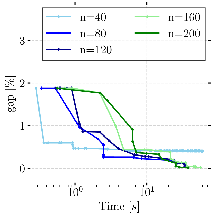
(a) Line profits

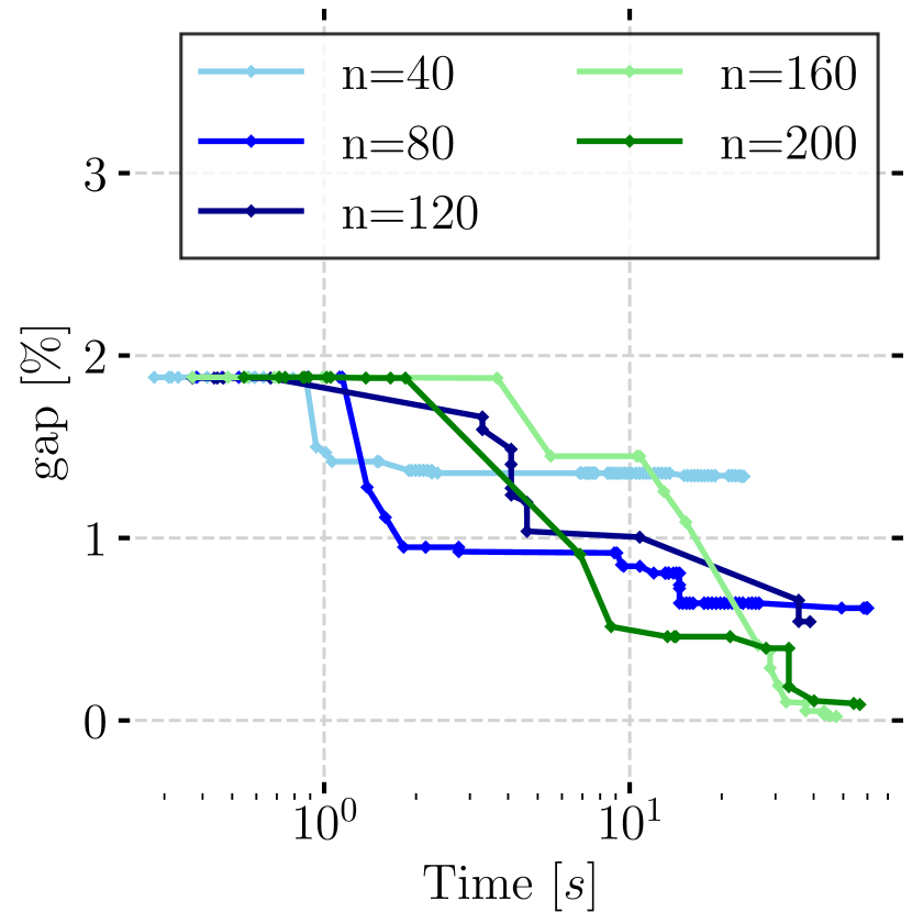
(b) Price difference

(c) Total cost derivative

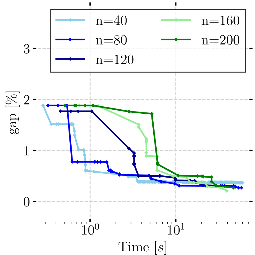
(d) PDTF-weighted

Figure 1: This figure depicts the solution process of solving rOTSP-Model-3 on the 1354_pegase case with different numbers of switchable lines $n=\lvert\mathscr{E}^{S}\rvert$, using Gurobi. Additionally, we compare solver performance, using differnt switching criteria to select lines $e\in\mathscr{E}^{S}$. Every marker represents an integer-feasible solution being found.

We derive an arbitrarily restrictable OTSP formulation (rOTSP-Model-3). The idea is to solve a reduced version of the OTSP that has less number of available topology control actions. The rOTSP-Model-3 is equal to sDCOPF-Model-2, if fully restricted to a specific $\mathscr{E}^{A}$. Without any restrictions, rOTSP-Model-3 is equal to OTSP-Model-1. To achieve the desired behaviour, we must introduce a second set $\mathscr{E}^{S}$ of switchable transmission lines. If line $e\in\mathscr{E}^{S}$, then line $e$ is available for switching. In general, not all lines are subject to switching. We want to be able to utilize knowledge of any incumbent topology $\mathscr{E}^{A}$. To derive a model, we use sDCOPF-Model-2 as a baseline. If a line $e$ should now be subject to switching, a variable $x_{e}$ and two constraints of type (1c) and (1d) must be attached. If $e\in\mathscr{E}^{A}$, we must make sure that a constraint (2c) is not additionally attached to the model. Applying this to all lines in a set $\mathscr{E}^{S}$ yields rOTSP-Model-3:

Model 3 Restrictable OTSP: rOTSP($\mathscr{E}^{A}$, $\mathscr{E}^{S}$) [MILP]

$$\min z_{3}=\sum_{\mathscr{G}}c_{g}(p_{g}),$$ s.t.: (4a)

$$\sum_{\mathscr{E}^{f}_{v}\cap\mathscr{E}^{A}}f_{e}-\sum_{\mathscr{E}^{t}_{v}\cap\mathscr{E}^{A}}f_{e}=\sum_{\mathscr{G}_{v}}p_{g}-d_{v}, \forall\text{ }v\in\mathscr{V}$$ (4b)

$$b_{e}(\theta_{v^{f}_{e}}-\theta_{v^{t}_{e}})=f_{e}, \forall\text{ }e\in\mathscr{E}^{A}\backslash\mathscr{E}^{S}$$ (4c)

$$b_{e}(\theta_{v^{f}_{e}}-\theta_{v^{t}_{e}})+(1-x_{e})M_{e}\geq f_{e}, \forall\text{ }e\in\mathscr{E}^{S}$$ (4d)

$$b_{e}(\theta_{v^{f}_{e}}-\theta_{v^{t}_{e}})\leq f_{e}+(1-x_{e})M_{e}, \forall\text{ }e\in\mathscr{E}^{S}$$ (4e)

$$-\overline{f}x_{e}\leq f_{e}\leq\overline{f}x_{e}, \forall\text{ }e\in\mathscr{E}^{S}\quad$$ (4f)

$$-\overline{f}\leq f_{e}\leq\overline{f}, \forall\text{ }e\in\mathscr{E}^{A}\backslash\mathscr{E}^{S}$$ (4g)

$$\underline{p}_{g}\leq p_{g}\leq\overline{p}_{g}, \forall\text{ }g\in\mathscr{G}$$ (4h)

$$\underline{\theta}\leq\theta_{v}\leq\overline{\theta}, \forall\text{ }v\in\mathscr{V}$$ (4i)

$$x_{e}\in\{0,1\}, \forall\text{ }e\in\mathscr{E}^{S}$$ (4j)

Constraints (4c) and (4g) are inferred from sDCOPF-Model-2, whereas (4d), (4e) and (4f) are used in OTSP-Model-1 in the same manner. The resulting formulation meets all requirements defined in section I-B. We can start searching for improved solutions taking advantage of arbitrary incumbent topologies $\mathscr{E}^{A}$, whilst keeping the constraint matrix compact as constraints and variables are not created for line $e$, iff $e\notin\mathscr{E}^{A}\cup e\notin\mathscr{E}^{S}$. Furthermore, switching decisions can be changed for line $e$, iff $e\in\mathscr{E}^{S}$. Lastly, the formulation allows us to form OTSP-Model-1 whereby a global optimum can be found by exact methods in a finite number of steps. It can be noted, that $\mathscr{E}^{S}\cap\mathscr{E}^{A}$ is regularly non-empty. Several important properties of rOTSP-Model-3 must be stated, as these are the foundation of our algorithm.

Observation 1.

rOTSP-Model-3 equals OTSP-Model-1, if $\mathscr{E}^{S}=\mathscr{E}$. rOTSP-Model-3 equals sDCOPF-Model-2, if $\mathscr{E}^{S}=\emptyset$.

Note, that rOTSP-Model-3 is a MILP. Thus, as we increase the size of the set of switchable lines, $n=\mathbf{card}(\mathscr{E}^{S})$, the complexity of the model increases. However, it was found [13] that only a small set of lines can induce most (or all) of the cost reduction benefits. Similarly to the previous sDCOPF-Model-2 model, we can build feasible solutions for OTSP-Model-1.

Remark 2 (Feasible Solution Construction from rOTSP-Model-3).

If a solution $(p^{*},f^{*},\theta^{*},x^{*})$ exists for the rOTSP-Model-3, then $(p^{*},f^{\prime\prime},\theta^{*},x^{\prime\prime})$, is a feasible solution for the OTSP-Model-1, where $f^{\prime\prime}$, and $x^{\prime\prime}$ are computed as follows:

$$\footnotesize x^{\prime\prime}_{e}=\begin{cases}x_{e}^{*},&e\in\mathscr{E}^{S}\\ \boldsymbol{1}_{\mathscr{E}^{A}}(e),&e\notin\mathscr{E}^{S}\\ \end{cases},~{}f^{\prime\prime}_{e}=\begin{cases}f_{e}^{*},&e\in\mathscr{E}^{S}\\ \begin{cases}f^{*}_{e},e\in\mathscr{E}^{A}\\ 0,e\notin\mathscr{E}^{A}\end{cases},&e\notin\mathscr{E}^{S}.\end{cases}$$ (5)

Two important properties related to the objective value $z_{3}$ of rOTSP-Model-3, namely, upper bound and monotonicity, can be inferred from the respective model and Observation 1. Both properties, like the previously mentioned, are of great importance to the data exchange at runtime and, hence, facilitate the architecure as well as resulting speedups. We state these properties as remarks, as they must be mentioned for later reference but should be obvious without a proof.

Remark 3 (Upper Bound).

Given a solution from rOTSP-Model-3, it holds that $z_{1}^{*}\leq z_{3}^{*}$ for any set $\mathscr{E}^{S}$.

Remark 4 (Monotonicity Property).

Let $\mathscr{P}_{1},\mathscr{P}_{2}$ be two instances of the rOTSP-Model-3, constructed using the sets $\mathscr{E}^{A}$ and $\mathscr{E}_{\mathscr{P}_{1}}^{\text{S}}$ and $\mathscr{E}_{\mathscr{P}_{2}}^{\text{S}}$, respectively, for each problem instance. If $\mathscr{E}^{S}_{\mathscr{P}_{1}}\subseteq\mathscr{E}^{S}_{\mathscr{P}_{2}}$, then $z^{*}_{3}(\mathscr{E}^{A},\mathscr{E}_{\mathscr{P}_{2}}^{\text{S}})\leq z^{*}_{3}(\mathscr{E}^{A},\mathscr{E}_{\mathscr{P}_{1}}^{\text{S}})$.

Given the aforementioned properties, the optimal objective values of the constructed problems are progressively closer to the optimal objective value of the original problem OTSP-Model-1, with an increasing $n$ (number of switchable lines). However, our heuristic relies on the fact that often only a couple of lines must be switchable (included into $\mathscr{E}^{S}$) to achieve close-to-optimal solutions. To identify candidate lines several methods were proposed in the literature, which are discussed and compared in the following section.

II-C Selecting candidate lines for transmission switching

To use rOTSP-Model-3, we must construct a set $\mathscr{E}^{S}$. We want to include only lines for switching that decrease operational costs. The cardinality of $\mathscr{E}^{S}$ is a direct driver of computational complexity of the resulting rOTSP-Model-3. To identify candidate lines, four switching criteria have been proposed in the literature: The line profits switching criterion (lpsc) as proposed in [11] and [14] is derived using KKT-conditions and expressed as:

$$\alpha_{e}=f^{*}_{e}(\pi^{*}_{v^{f}_{e}}-\pi^{*}_{v^{t}_{e}}).$$ (6)

Additionally, a price difference, total cost derivative and PTDF-weighted cost derivative switching criterion were proposed in [14]. Removing a candidate line based on these criteria does not guarantee improvements due to the problem being discrete in nature. Removing a line might render a problem infeasible. Deriving indicators for all lines facilitates to create a sorted list $\mathbb{L}$, in ascending order, by the lines’ respective switching criterion (highest reduction first). All criteria can be computed based on sDCOPF-Model-2 and its dual variables. Based on $\mathbb{L}$, we create a subset of switchable lines $\mathscr{E}^{S}$, by selecting the $n$ first lines in $\mathbb{L}$. To illustrate the effect of different heuristics and size of switching lines set, we tested all switching criteria using rOTSP-Model-3 with different values for $n$. Results for the 1354_pegase case are displayed in Figure 1. Results indicate, that the lpsc performs best. Especially for smaller sets of switchable line, the improvements to be achieved are higher than with other criteria. The total cost derivative switching criterion also yields similar results, but only for larger sets $\mathscr{E}^{S}$ ($n=160,~{}n=200$). The total cost derivative and PDTF-weighted criteria in Figure 1(c) and 1(d) do not produce comparable improvements and are more expensive to compute as they require the PDTF and LODF respectively.

III Algorithmic Architecture and Parallel Implementation

III-A Parallel Framework

As a framework for parallel high-performance computing, the open-source implementation message passing interface chameleon (MPICH) is used. This tool facilitates to define independent processes (also called ranks), implement communication, and allocate resources. In our design, multiple ranks can be defined 0 and $\{1,\dots,j\,\ldots,|\mathscr{J}|\}$. We reserve rank 0 for the principal worker, the main solution process. Information is exchanged between rank 0 and the others asynchronously. Whereas rank 0 receives new solutions from a rank $j$, the global incumbent and information on the solution process is sent from rank 0 to all $j\in\mathscr{J}$ continuously. To implement advanced solver behaviour (including communication), Gurobi’s user callbacks are utilized. Callbacks facilitate online communication between external software and the MIP solver, i.e., sending and retrieving data during runtime. Here, external software might also mean an independent instance of the same MIP solver. Calling user functions is possible during different times of the iterative solution process, after exploring a MIP node or finding a new solution for example. While parallel implementations might require a process that assigns workloads [22], callbacks and functions implemented in MPI allow for completely asynchronous behaviour, with optimizers running on all ranks.

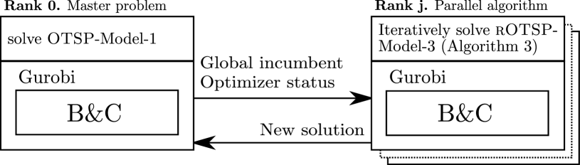
Figure 2: Parallel coordination

Figure 2 represents a simplified version of the implemented parallel coordination and data exchange. The coordination can be summarized as follows: while solving OTSP-Model-1, we solve instances of rOTSP-Model-3 in parallel. Since rOTSP-Model-3 can be constructed with a reduced number of integer variables, feasible solutions can be obtained quicker. If a solution is obtained on any rank, we convert it to a solution of OTSP-Model-1 (see remark 2) and send it to rank 0. It may occur, that the solver instance on rank 0 attained an upper bound that is better than any solution expected to be produced by rOTSP-Model-3 on a rank j. In this case, we send the superior solution (global incumbent) to rank j, build a new instances of rOTSP-Model-3 and continue the process. The parallel algorithm terminates after reaching the time limit or obtaining an optimal solution on rank 0. Then again a signal is sent to all workers to stop optimization. In the next subsection, we present the parallel algorithm in detail.

III-B Parallel Algorithm (Rank $j$)

The main goal of our parallel algorithm is to supply strong solutions for OTSP-Model-1 as fast as possible. This (feasible) solution might update the upper bound of the OTSP in rank 0. To keep algorithms concise, several technical remarks must be made on how communication is implemented. When sending data using MPI, tags are set to facilitate identification of data. In the proposed architecture 3 pieces of information are exchanged and must be identified: Optimizer (termination) status information on rank 0 will in the following be referred to as stat., solutions produced on rank j by sol.and global incumbents by inc.. A pseudo code call Recv(src, tag) entails probing for data of type tag sent from source src, to then receive it if it is available. Similarly, a call Send(data, dst, tag) means that data is sent to destination dst. On several occasion we also wait for requests to be completed. Moreover, let $\mathbb{c}$ denote all the parameters related to a test case. Our algorithm is executed on ranks j and consists of three major components: (i) initialization, (ii) prioritization, and (iii) solving restricted rOTSP instances.

III-B1 Initialization

As described, we are reliant on a feasible set $\mathscr{E}^{A}$. Such a set’s feasibility can be validated by solving sDCOPF-Model-2. From the obtained solution, we are able to build a feasible solution for OTSP-Model-1, as described in (3) and derive dual values. The procedure is summarized in Algorithm 1. Note that $x^{\prime}$ is used as a mipstart (initialization of binary variables) in subsequent steps (Algorithm 3).

Input : $\mathbb{c}$, $\mathscr{E}^{A}$

$(p^{*},f^{*},\theta^{*},\pi^{*})$ $\leftarrow$ solve sDCOPF-Model-2 ($\mathbb{c}$, $\mathscr{E}^{A}$)

$(f^{\prime},x^{\prime})$ = Generate feasible solution (Rem. (3))

Output : $(p^{*},f^{\prime},\theta^{*},x^{\prime},\pi^{*})$

Algorithm 1 Initialization Procedure

III-B2 Prioritization of line selection for switching

Based on the results presented in section II-C, the lpsc criterion is chosen for line prioritization. To compute priority value $\alpha_{e}$ based on (II-C), LMPs $\pi^{*}$ and power flow values $f^{*}$ must be obtained by solving sDCOPF-Model-2. Algorithm 2 describes how we build a priority list $\mathbb{L}$, based on the lpsc derived from sDCOPF-Model-2.

Input : $\mathbb{c}$, $\mathscr{E}^{A}$, $n$

/* Note, that $\pi^{*}$ and $f^{*}$ only exist if sDCOPF-Model-2 ($\mathbb{c},~{}\mathscr{E}^{A}$) has a solution. */

$(p^{*},f^{\prime},\theta^{*},x^{\prime},\pi^{*})\leftarrow\textsc{Algorithm 1}(\mathbb{c},\mathscr{E}^{A}$)

$\alpha=0^{\lvert\mathscr{E}\rvert}$, $\mathscr{E}^{S}=\emptyset$

for $e\in\mathscr{E}$ do

       /* Any (switching) criterion can be used. */

       $\alpha_{e}=f^{\prime}_{e}(\pi^{*}_{v^{f}_{e}}-\pi^{*}_{v^{t}_{e}})$

$\mathbb{L}$ $=$ sort($\mathscr{E}$, by $\alpha$, ascending)

$\mathscr{E}^{S}\leftarrow\mathbb{L}_{1,\dots,n}$

Output : $\mathscr{E}^{S}$

Algorithm 2 Line Prioritization

III-B3 Solving reduced OTSP instances

Algorithm 3 shows how information from each rank is exchanged to speed up both B&B algorithms. We use R0 and Rj to refer to rank 0 and rank j, respectively.

Algorithm 3 is running as long as the master problem OTSP-Model-1 is running. A binary variable root_process_terminated indicates whether solving the master problem is still ongoing. Its state, along with the global incumbent, is continuously sent from rank 0. The solution process on rank 0 is terminated upon reaching a time limit or obtaining an optimal solution.

The input of Algorithm 3 is the electric grid data and parameters $n\in\mathbb{N}^{\text{+}}$ (number of switchable lines to be added to the set $\mathscr{E}^{S}$) and $\Delta{n}\in\mathbb{N}^{\text{+}}$ (number of new lines to added to the set $\mathscr{E}^{S}$ after every iteration). The parameter update_time (time window to retrieve the global incumbent from rank 0 - fixed to 10s in our case) and reset_time (time window to check if no better solution than rank 0 can be found in rank 1- fixed to 20 s in our case) must be set as well.

Algorithm 3 starts with the initialization of sets of switchable lines $\mathscr{E}^{S}=\emptyset$ and active lines $\mathscr{E}^{A}=E$. Based on $\mathscr{E}^{A}$ a mipstart is generated for rOTSP-Model-3 using Algorithm 1 as well as priority list $\mathbb{L}$ using Algorithm 2. Then, iteratively, we solve rOTSP-Model-3 and pass its solutions to the main B&C instance at rank 0.

Input : $\mathbb{c}$, $n$, $\Delta{n}$

update_time, reset_time

Initialize :  $\mathscr{E}^{A}=\mathscr{E}$

$(p^{*},f^{\prime},\theta^{*},x^{\prime},\pi^{*})\leftarrow\textsc{Algorithm 1}(\mathbb{c},\mathscr{E}^{A})$

Send($(p,f^{\prime},\theta,x^{\prime})$, R0, sol.)

mipstart $=x^{\prime}$

$\mathscr{E}^{S}\xleftarrow{}$ Algorithm 2 ($\mathbb{c},\mathscr{E}^{A},n$)

while !root_process_terminated[1] do

       /* (a) Retrieve global incumbent from rank 0, if available */

       $(ub^{\textbf{R0}},p^{\textbf{R0}},f^{\textbf{R0}},\theta^{\textbf{R0}},x^{\textbf{R0}})$ = Recv(R0, inc.)

       $\mathscr{E}^{A}$ = $\{e\in\mathscr{E}\mid x_{e}^{\textbf{R0}}=1\}$

       mipstart $=$ $(\boldsymbol{1}_{\mathscr{E}^{A}}(e_{1}),\dots,\boldsymbol{1}_{\mathscr{E}^{A}}(e_{\lvert\mathscr{E}^{S}\rvert}))$

       /* (b) Construct rOTSP-Model-3 with current $\mathscr{E}^{A}$ and $\mathscr{E}^{S}$, and call B&C optimization. */

       solve(rOTSP-Model-3 ($\mathbb{c},\mathscr{E}^{A}$,$\mathscr{E}^{S}$, mipstart))

       while solving rOTSP-Model-3 do

             /* (c) Update global incumbent from rank 0 every update_time. Get information about if rank 0 returned. */

             if update_time_passed then

                   $(ub^{\textbf{R0}},p^{\textbf{R0}},f^{\textbf{R0}},\theta^{\textbf{R0}},x^{\textbf{R0}})$ = Recv(R0, inc.)

                   root_process_terminated = Recv(R0, stat.)

                  

            /* (d) Reset rOTSP-Model-3 B&C if $lb^{\textbf{Rj}}\geq ub^{\textbf{R0}}$ */

             if reset_time_passed then

                   if Condition in (d) met then

                         Stop B&C of rOTSP-Model-3

                        

                  

            /* (e) Send feasible solution to rank 0 when new MIP solution, $x^{\textbf{Rj}}$, is found in rOTSP-Model-3 with objective value $z^{\textbf{Rj}}$ better than $ub^{\textbf{R0}}$ */

             if New sol. found $\land$ $z^{\textbf{Rj}}<ub^{\textbf{R0}}$ then

                   $(p,f^{\prime\prime},\theta,x^{\prime\prime})$ $\xleftarrow{}$ Generate feasible solution from (5)

                   Send($(p,f^{\prime\prime},\theta,x^{\prime\prime})$, R0, sol.)

                  

            

      /* (f) Update $\mathscr{E}^{S}$ */

       $n=\min\{n+\Delta{n},\lvert\mathscr{E}\rvert\}$

       $\mathscr{E}^{A}$ = $\{e\in\mathscr{E}\mid x_{e}^{\textbf{R0}}=1\}$

       $\mathscr{E}^{S}\leftarrow{}$ Algorithm 2 ($\mathbb{c},\mathscr{E}^{A},n$)

      

Algorithm 3 Priority-Guided Heuristic

While solving rOTSP-Model-3, six main tasks are performed. Three out of six are in the scope of the implemented callback function. They are described as follows.

Retrieving global incumbent from rank 0, if available

Rank 0 continuously sends the incumbent on OTSP-Model-1. If an incumbent was sent, it is received by rank j and used to update mipstart, $\mathscr{E}^{A}$ and information on the global ub at rank 0 saved by rank j, $ub^{\textbf{R0}}$.

Reconstruction of rOTSP-Model-3 with updated set information for $\mathscr{E}^{A}$, $\mathscr{E}^{S}$ and mipstart

. First, rOTSP-Model-3 is loaded into a MIP solver (Gurobi in our case). On loading the model, a callback function is attached. This function performs 3 main behaviours, dependent on the current solver state.

Update the global incumbent retrieved from rank 0 every update_time

In regular intervals, it is checked whether a new incumbent was sent from R0. If so, Rj receives it and updates its global incumbent information. This information is vital to control the behaviour of worker ranks. Upper bound $ub^{\textbf{R0}}$ is required, for example, to determine if better solutions can still be found on rank j with the current instance of rOTSP-Model-3, step (d).

Reset the B&C algorithm at rank j

We utilize 2 criteria to abort optimization of our MIP heuristic. These conditions are evaluated continuously after an interval of length reset_time has passed. First, $lb^{\textbf{Rj}}\geq ub^{\textbf{R0}}$ means that no new incumbents can be produced by our MIP heuristic. If that condition is met or no improvements were found during the last 20 s, we terminate optimization and go to step (f).

Send feasible solution to rank j

Whenever a feasible solution is found for rOTSP-Model-3 during B&C exploration or internal heuristics, it is converted (according to (5)) and sent to rank 0. Rank 0 then updates its incumbent based on this solution, if $z^{\textbf{Rj}}<ub^{\textbf{R0}}$.

Update $\mathscr{E}^{S}$

Finally, the ordered list of switching lines $\mathbb{L}$ is updated. The new set of candidate lines for switching control is updated taking the first $n$ lines. The number of lines $n$ is increased after each iteration by $\Delta{n}$. Eventually, in the worst case, $n$ could be equal to the set of all lines, and recover OTSP-Model-1.

IV Numerical Experiments

IV-A Test cases and setup

Hard- and software-wise, our test system has 16 GB of RAM and is equipped with an i7-7820X, clocked at 4.0 GHz. As all experiments were run with hyper-threading disabled, a total of 8 logical cores were available. The software used is depicted in Table II.

TABLE II: Summary of the software used

App/Pkg	Gurobi	MPICH	Julia	JuMP.jl	Gurobi.jl	MPI.jl
Version	9.1.2	4.3.1	1.6.3	0.21.2	0.9.14	0.19.1

For all experiments the pglib-opf library was used. We set $\underline{p}=\boldsymbol{0}$. Software for managing data files and running our experiments was written in Julia Language.

IV-B Computational performance with consistent parameters

TABLE III: Experimental results

				OTSP, no mipstart			$\textsc{OTSP}_{\boldsymbol{x}\boldsymbol{0}}$, mipstart			P-OTSP
#	Case	# buses	# lines	ct [s]	gap [%]	$\Delta z$ [%]	ct [s]	gap [%]	$\Delta z$ [%]	ct [s]	gap [%]	$\Delta z$ [%]	$\overline{\Delta z}[\$/h]$
1	118_ieee	118	186	0.72	0.0${}^{\text{+}}$	13.491	1.53	0.0${}^{\text{+}}$	13.491	1.82	0.0${}^{\text{+}}$	13.491	0.0
2	588_sdet	588	686	900	0.064	2.14	900	0.022	2.19	900	0.039	2.17	-36.65
3	1354_pegase	1354	1991	900	0.04	1.938	900	0.1	1.882	192.03	0.007${}^{\text{+}}$	1.971	364.13
4	1888_rte	1888	2531	369	0.0092${}^{\text{+}}$	-0.0092	0.39	0.0${}^{\text{+}}$	0.0	2.03	0.0${}^{\text{+}}$	0.0	0.0
6	2383_wp_k	2383	2896	900	-	-	900	0.18	4.05	900	0.02	4.21	2732.38
7	2736_sp_k	2736	3504	900	0.07	6.82	900	0.65	6.21	900	0.04	6.86	355.1
8	2746_wop_k	2746	3514	900	-	-	900	0.19	10.24	494.5	0.003${}^{\text{+}}$	10.46	2094.06
9	2869_pegase	2869	4582	900	-	-	900	0.39	1.07	900	0.18	1.27	4817.47
10	3012wp_k	3012	3572	900	0.54	8.01	900	0.44	8.11	900	0.31	8.22	2870.06
11	3120sp_k	3120	3693	900	0.7	6.52	900	0.9	6.4	900	0.29	6.77	5510.58
12	3375sp_k	3375	4161	900	1.34	3.15	900	1.17	3.32	900	0.86	3.62	19966.29
13	6470_rte	6470	9005	900	-	-	900	8.83	4.39	900	5.32	7.46	55207.37
14	13659_pegase	13659	20467	900	-	-	900	0.88	0.0	900	0.42	0.46	31022.55

${}^{\text{+}}$ The solution is classified optimal as gap $\leq 0.01$.

Figure 3: This plot shows the solution process on the 1354_pegase test case, utilizing different solution strategies. Both baseline methods (OTSP and $\textsc{OTSP}_{\boldsymbol{x0}}$) do not find an optimal solution within the the time limit of 900 s. Supplying a mipstart $x_{0}$ has a notable effect on solutions that can be obtained, especially early on. Using our parallel implementation (P-OTSP) an optimal solution is found in less than 193 s. The plot shows ub, lb of the P-OTSP procedure, as well as whether a solution was produced by the solver instance working on the full problem (P-OTSP, sol., r.0) or a MIP heuristic (P-OTSP, sol., r.1). We furthermore depict, whether a full iteration was completed by Algorithm 3 (P-OTSP, itr., r.1). At around 45 s, optimization on rank 1 restarts (iteration) due to no solutions being found. We can see that right after restarting optimization from a different $x^{\textbf{R0}}$, new solutions are found quickly.

We first want to verify, that our method can produce improvements on a multitude of test cases with consistent setting. For the following experiments we used two ranks, $\mathscr{J}=\{1\}$. Using affinity maps, we pinned rank 0 to cores 0-3 and rank 1 to cores 4-7. As parameters for Algorithm 3, $n=40$ and $\Delta n=10$ were chosen. We set a time limit of 15 minutes. Three exact solution strategies were implemented for solving each test case. These are described in the following:

• OTSP, no mipstart. We solve OTSP-Model-1 using Gurobi with default settings. No mipstart is provided. Gurobi has available all logical cores (8).

• $\textsc{OTSP}_{\boldsymbol{x}\boldsymbol{0}}$, mipstart. We solve OTSP-Model-1 using Gurobi with default settings. An initial solution is generated from Algorithm 1 and passed to Gurobi as mipstart. Gurobi has available all logical cores (8).

• P-OTSP. In this case, we use the parallel architecture introduced in section III.

Table III shows the results of solving 14 test cases utilizing the three aforementioned strategies. The experiment id, the name of the test case as well as the number of buses and lines are shown in columns 1-4. All lines are considered switchable. Thus, the number of lines also denotes the number of integer variables of each problem. The smallest grid has 118 buses and 186 lines, while the largest grid has 13659 buses and 20467 lines. Furthermore, solutions with $\textit{gap}\leq 0.01\%$ are classified as optimal. For the non-optimal cases, optimization is terminated upon reaching the time limit. For each of the three solution strategies, we report the computational time ct), relative optimality gap and relative cost reduction ($\Delta z$) of the OTSP over a linear DC approximation with all lines active. In addition, we report the absolute cost reduction of P-OTSP over either OTSP or $\textsc{OTSP}_{\boldsymbol{x}\boldsymbol{0}}$, depending on which performed better ($\overline{\Delta z}$).

For small test cases (such as #1, #2 and #4), performance improvements might not be achieved. For the 118-bus case, optimization takes less than 2 seconds until an optimal solution is found. Using optimization packages as illustrated in Table II, we add additional code and therefore run and compile time to the solution process. This becomes less insignificant as the problems are more difficult to solve. On cases as large as the 588_sdet-bus case, Gurobi still does not benefit from the proposed solution technique. However, our method also does not harm the performance significantly either. This generally starts changing with the 1354-bus case. Case #4 is large as well, but $\mathscr{E}^{A}=\mathscr{E}$ is an optimal topology. Our method also has no significant effect, as a certificate of optimality can be attained very quickly.

For larger cases starting with the 1354-bus case, significant improvements in performance or solution quality can be observed. Figure 3 depicts the solution process. While baseline methods yield good solutions with a low final gap of 0.04% and 0.07% respectively, after reaching the time limit of 900 s, P-OTSP finds an optimal solution after 192.03 s. With a final gap of 0.007% the difference to both other solution methods seems small, but is significant in absolute terms with 364.13 [$/h]. Figure 3 shows that much better solutions are found during the first 100 s. Solutions are found by Gurobi’s heuristics on rank 0 and rank 1. Whenever good solutions are supplied, further improvements can quickly be obtained based on them. Throughout the optimization process, Algorithm 3 performs 3 full iterations, which are displayed in vertical blue lines. This is due to better incumbents being available on rank 0, finding an optimal solution for a particular instance of rOTSP-Model-3 or not having found any solution within the last 20 seconds.

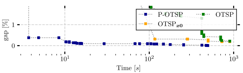
(a) 2746wop_k

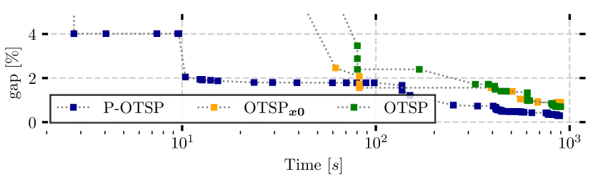
(b) 3120sp_k

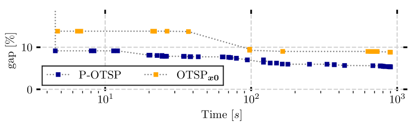
(c) 6470_rte

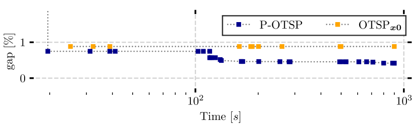
(d) 13659_pegase

Figure 4: In this figure, the solution process of 4 additional test cases is illustrated. We plot the gap for OTSP, $\textsc{OTSP}_{\boldsymbol{x}\boldsymbol{0}}$ and P-OTSP. Every marker denotes obtaining an integer-feasible solution. For larger problems the MIP solver is not able to find a feasible to find a solution within the time limit. We can reliably obtain better solutions.

Figures 4 depict the progress on 4 additional test cases, again for each solution strategy. Figure 4(a) shows the progress on the largest case an optimal solution can be obtained for, within the time limit. The progress of the different methods is similar to that on the 1354-bus case. Without a mipstart solution, it takes much longer until good solutions can be achieved. Our parallel framework not only finds an optimal solution, but extremely good solutions very early on. In this case, a cost reduction of 2094.06 $[\$/h]$ can be achieved.

While solving the 3120-bus case, $\textsc{OTSP}_{\boldsymbol{x}\boldsymbol{0}}$ is slightly ahead at around 90 s, due to a strong solution supplied by an internal heuristic. We observe, however, that P-OTSP improves on solutions much faster, which results at a final total improvement of 5510.58 $[\$/h]$, over the best competing method. The last displayed test cases 6470_rte (Fig.4(c)) and 13659_pegase (Fig. 4(d)) show very similar solution processes. Without a mipstart, Gurobi cannot find a solution within the time limit. Providing a start solution results in multiple further improvements. P-OTSP outperforms a single solver instance significantly on both cases. Due to the fact that these systems are large and P-OTSP finds significantly better solutions, absolute cost reductions are 55207.37 $[\$/h]$ and 31022.55 $[\$/h]$ over competing methods. On a general note, significant improvements can be produced utilizing P-OTSP.

IV-C Performance using multiple worker ranks

During the previously described experiments, we only used 1 worker rank, solving a single instance of rOTSP-Model-3 at a time. Figures 1 show, however, that small sets of switchable lines ($n=40$) result in fast improvements, whilst larger sets ($n=200$) result in very good solutions. The advantages of a higher degree of parallelization are studied on the 1354_pegase test case. We now run 1, 2 and 3 worker ranks in parallel to our master problem, each with a different parameter $n_{1}=40,~{}n_{2}=120$ and $n_{3}=200$. With 2 worker ranks, we pin the root rank to 4 cores and each worker rank to 2, whilst with 3 worker ranks, each rank is pinned to 2 cores. We compare our results to $\textsc{OTSP}_{\boldsymbol{x}\boldsymbol{0}}$ as well.

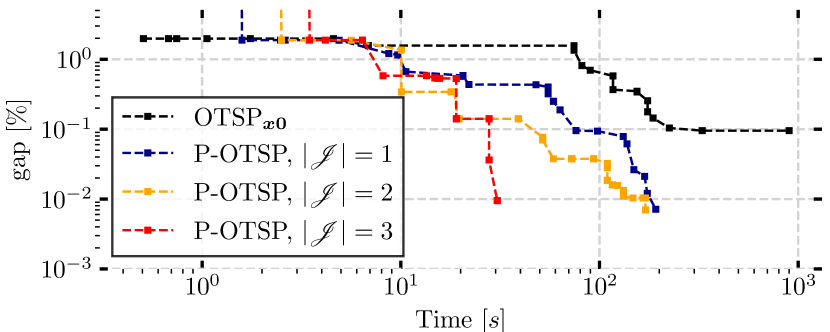
Figure 5: Here, the solution process utilizing varying numbers of parallel ranks is compared, on the 1354_pegase test case. Every marker denotes obtaining an integer-feasible solution. We use $\textsc{OTSP}_{\boldsymbol{x}\boldsymbol{0}}$ as a baseline and compare it to P-OTSP with 1, 2 and 3 parallel worker processors. We obtain significant improvements.

Figure 5 impressively shows, that performance, in terms of solution speed and solution quality, improves as more parallel solver instances are utilized. The total number of cores (eight) is the same for all four experiments with different parallel architecture. Our parallel algorithm shows to utilize those more efficiently, when compared to the stock solver. While $\textsc{OTSP}_{\boldsymbol{x}\boldsymbol{0}}$ cannot find an optimal solution within the time limit, P-OTSP ($\lvert\mathscr{J}\rvert=3$) finds an optimal solution within 30 s. This means more than 6 times lower computations times when compared to P-OTSP ($\lvert\mathscr{J}\rvert=1$ and $\lvert\mathscr{J}\rvert=2$) or more than 30 times lower computation times when compared to $\textsc{OTSP}_{\boldsymbol{x}\boldsymbol{0}}$. To outline the source of improvements better, we revisit an adjusted version of Figure 1(a), as Figure 6.

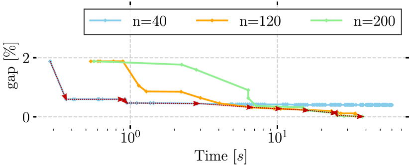
Figure 6: It can be observed, that the application of Gurobi’s internal heuristics is sensitive to $n$, just like in Figure 1. Whilst small values $n$ result in quick improvements, larger values yield close-to-optimal ones. With $\lvert\mathscr{J}\rvert=3$ we solve all 3 sub problems and the full OTSP simultaneously, sending all solutions immediately to the main optimizer instance on the root process. The red path shows an approximation of the progress our parallel algorithm makes.

V Conclusion

In this paper, we proposed a parallel framework to solve combinatorial optimization problems and studied its effectiveness on the optimal transmission switching problem, on 14 case studies. We furthermore, study performance improvements for an increased number of parallel processes, assessing the methods scalability. The results show that our parallel approach (P-OTSP) can efficiently harness the advantages of both, solving the full OTSP model formulation and heuristics likewise. A parallel implementation is advantageous over merely trying to generate improvements using heuristics, because the lower bound on the full problem is available during run time, whereby optimality can be assessed. The proposed parallel architecture is compatible with any existing MILP solver, such as Gurobi, CPLEX, Xpress and SCIP - to name a few. Problem-specific switching criterion like lpsc has shown very effective when it is used in heuristics that run in parallel to the main OTSP solution procedure. Problem-specific switching criterion like lpsc has shown effective when used in a heuristic method that runs parallel to the main OTSP solution procedure. The computational efficiency enhancement materialized by supplying strong solutions that accelerate B&C algorithms of off-the-shelve solvers.

The optimality gap reported for the 14 case studies, shows that, except for the 6470_rte case, solutions within 0.86% of of the full OTSP’s globally optimal objective value’s can be obtained in less than 15 minutes. Even if an optimal solution cannot be obtained within the time limit, significantly better solutions are available.

Lastly, a high degree of parallelization can reduce computation times by a factor of 30. The framework proposed is not limited to any particular heuristic or problem. Instead of MIP solvers, heuristics could be run in parallel. A direction for future work is the application of the proposed methods to different discrete problems in power systems. Moreover, generating a priority list $\mathbb{L}$ could be done using different rules or machine learning algorithms. The potential is huge and goes beyond the optimal transmission switching problem. Many combinatorial problems are repeatedly solved in practice, domain-specific knowledge, data-driven algorithms, or machine learning could help to accelerate exact algorithms. A final implication is this; approaching transmission switching in the presented manner might provide strategic implications for practitioners. The solutions obtained not only provide improvements but also theoretical guarantees as to how much improvement is still possible. It poses a stronger basis for future decisions than cost reduction alone.

References

- [1] H. Glavitsch. Switching as means of control in the power system. International Journal of Electrical Power & Energy Systems, 7(2):92 – 100, 1985.
- [2] A. A. Mazi, B. F. Wollenberg, and M. H. Hesse. Corrective control of power system flows by line and bus-bar switching. IEEE Transactions on Power Systems, 1(3):258–264, 1986.
- [3] Wei Shao and V. Vittal. Corrective switching algorithm for relieving overloads and voltage violations. IEEE Transactions on Power Systems, 20(4):1877–1885, 2005.
- [4] E. B. Fisher, R. P. O’Neill, and M. C. Ferris. Optimal transmission switching. IEEE Transactions on Power Systems, 23(3):1346–1355, 2008.
- [5] K. W. Hedman, R. P. O’Neill, E. B. Fisher, and S. S. Oren. Optimal transmission switching with contingency analysis. IEEE Transactions on Power Systems, 24(3):1577–1586, 2009.
- [6] C. Liu, J. Wang, and J. Ostrowski. Static switching security in multi-period transmission switching. IEEE Transactions on Power Systems, 27(4):1850–1858, 2012.
- [7] A. Khodaei, M. Shahidehpour, and S. Kamalinia. Transmission switching in expansion planning. IEEE Transactions on Power Systems, 25(3):1722–1733, 2010.
- [8] J.C. Villumsen and A.B. Philpott. Investment in electricity networks with transmission switching. European Journal of Operational Research, 222(2):377 – 385, 2012.
- [9] Raphael Saavedra, Alexandre Street, and José M. Arroyo. Day-ahead contingency-constrained unit commitment with co-optimized post-contingency transmission switching. IEEE Transactions on Power Systems, 35(6):4408–4420, 2020.
- [10] K.Lehmann, A. Grastien, and P. Van Hentenryck. The complexity of dc-switching problems. Technical report, NICTA, 2014.
- [11] J. D. Fuller, R. Ramasra, and A. Cha. Fast heuristics for transmission-line switching. IEEE Transactions on Power Systems, 27(3):1377–1386, 2012.
- [12] S. Fattahi, J. Lavaei, and A. Atamtürk. A bound strengthening method for optimal transmission switching in power systems. IEEE Transactions on Power Systems, 34(1):280–291, 2019.
- [13] C. Barrows, S. Blumsack, and R. Bent. Computationally efficient optimal transmission switching: Solution space reduction. In 2012 IEEE Power and Energy Society General Meeting, pages 1–8, 2012.
- [14] Pablo A. Ruiz, Justin M. Foster, Aleksandr Rudkevich, and Michael C. Caramanis. On fast transmission topology control heuristics. In 2011 IEEE Power and Energy Society General Meeting, pages 1–8, 2011.
- [15] F. Pourahmadi, M. Jooshaki, and S. H. Hosseini. A dynamic programming-based heuristic approach for optimal transmission switching problem with n-1 reliability criterion. In 2016 International Conference on Probabilistic Methods Applied to Power Systems (PMAPS), pages 1–7, 2016.
- [16] M. Soroush and J. D. Fuller. Accuracies of optimal transmission switching heuristics based on dcopf and acopf. IEEE Transactions on Power Systems, 29(2):924–932, 2014.
- [17] A. Papavasiliou, S. S. Oren, Z. Yang, P. Balasubramanian, and K. Hedman. An application of high performance computing to transmission switching. In 2013 IREP Symposium Bulk Power System Dynamics and Control - IX Optimization, Security and Control of the Emerging Power Grid, pages 1–6, 2013.
- [18] H. P. Young and S. Zamir. Handbook of Game Theory. Elsevier Science Inc., USA, 2015.
- [19] Chung-Yang Huang, Chao-Yue Lai, and Kwang-Ting Cheng. Fundamentals of Algorithms, pages 173–234. 12 2009.
- [20] Matteo Fischetti and Andrea Lodi. Heuristics in Mixed Integer Programming. John Wiley & Sons, Ltd, 2011.
- [21] F. Trespalacios and I. E. Grossmann. Review of mixed-integer nonlinear and generalized disjunctive programming methods. Chemie Ingenieur Technik, 86(7):991–1012, 2014.
- [22] Mahdi Namazifar and Andrew J. Miller. A parallel macro partitioning framework for solving mixed integer programs. In Laurent Perron and Michael A. Trick, editors, Integration of AI and OR Techniques in Constraint Programming for Combinatorial Optimization Problems, pages 343–348, Berlin, Heidelberg, 2008. Springer Berlin Heidelberg.