Longitudinal Magnetization and specific heat of the anisotropic Heisenberg antiferromagnet on Honeycomb lattice

Abstract

We study the effects of longitudinal magnetic field and temperature on the thermodynamic properties of two dimensional Heisenberg antiferromagnet on the honeycomb lattice in the presence of anisotropic Dzyaloshinskii-Moriya interaction and next nearest neighbor coupling exchange constant. In particular, the temperature dependence of specific heat have been investigated for various physical parameters in the model Hamiltonian. Using a hard core bosonic representation, the behavior of thermodynamic properties has been studied by means of excitation spectrum of mapped bosonic gas. The effect of Dzyaloshinskii-Moriya interaction term on thermodynamic properties has also been studied via the bosonic model by Green’s function approach. Furthermore we have studied the magnetic field dependence of specific heat and magnetization for various anisotropy parameters. At low temperatures, the specific heat is found to be monotonically increasing with temperature for magnetic fields in the gapped field induced phase region. We have found the magnetic field dependence of specific heat shows a monotonic decreasing behavior for various magnetic fields due to increase of energy gap in the excitation spectrum. Also we have studied the dependence of magnetization on Dzyaloshinskii-Moriya interaction strength for different next nearest neighbor coupling constant.

Department of Physics, Razi University, Kermanshah, Iran

Keywords: Longitudinal magnetization; Heisenberg model; Green’s function.

PACS: 73.22.-f; 72.80.Vp; 73.63.-b; 78.20.-e

1 Introduction

Quantum magnetism on geometrically two-dimensional frustrated spin systems with $S=1/2$ have lately received massive attentions, due to their potential for realizing the quantum spin liquid, a magnetically disordered state which respects all the symmetries of the systems, even at absolute zero temperature[1]. The spin model, recently attracted many interests, is the Heisenberg model with first and second antiferromagnetic exchange interaction in honeycomb lattice. In sufficiently low spin systems, the quantum mechanical zero point motion can forbid long range magnetic order and produce a quantum spin liquid state, a correlated state that breaks no symmetry and possesses topological properties, possibly sustaining fractionalized excitations[2, 3, 4, 5, 6]. Although the triangular lattice was first theoretically proposed by Anderson[2] as an ideal benchmark to search for the quantum spin liquid, it was soon found that the $S=1/2$ antiferromagnetic Heisenberg model on a triangular lattice is magnetically ordered with a $120^{0}$ arrangement of the spins. Despite the intense activity, only a small number of triangular materials have been identified as possible candidates for quantum spin liquid behavior such as th layered organic materials. Hence, there is a need to find evidence for quantum spin liquid behavior in more compounds. Honeycomb lattice materials have attracted lots of attention in recent years due to their interesting and poorly understood magnetic properties. Inorganic materials such as Na₂ Co₂TeO₆[7], BaM₂(XO₂)₂ (with X=As)[8], Bi₃Mn₄O₁₂(NO₃)[9] and In₃Cu₂VO₉[10] are examples of honeycomb lattice antiferromagnets in which the magnitude of the spin varies from $S=1/2$ in BaM₂(XO₄)₂ for M=Co to S=1 for M=Ni (with X=As) and to S=3/2 in Bi₃Mn₄O₁₂(NO₃). It is important then to understand theoretically the magnetic properties of interacting localized moments on the frustrated honeycomb lattice as has been previously done on triangular lattices. Although the numerical evidence for a quantum spin liquid in the half-filled Hubbard model on the honeycomb lattice[11] has been questioned[12], exact diagonalization studies on the $J_{1}-J_{2}$ Heisenberg model with $S=1/2$ have found evidence for short range spin gapped phases for $J_{2}=0.3-0.35$ suggesting the presence of a Resonance Valence Bond (RVB) state[13]. In the presence of external magnetic fields, finite temperature high resolution spectroscopies such as inelastic neutron scattering[14] and magnetic transport [15] have theoretically been calculated by dynamical correlation functions of the Heisenberg model on honeycomb lattice. Specially, field induced effects on the dynamical spin correlation function in low dimensional quantum spin models have been attracting much interest from theoretical and experimental point of view in recent years [16, 17, 18]. Spin-orbit coupling induces both symmetric and antisymmetric anisotropic properties or Dzyaloshinskii-Moriya spin anisotropy in the exchange coupling between nearest neighbour spins. A Dzyaloshiskii-Moriya (DM) interaction with a DM vector perpendicular to the layer produces an easy-plane spin anisotropic Hamiltonian for honeycomb lattice. DM interaction breaks $SU(2)$ symmetry of the model and reduces it to $U(1)$ symmetry around the $D$ vector. This DM interaction is believed to orient the spins in the 2D layer. For applied large magnetic fields ($B$) along perpendicular to the plane, the Zeeman term overcomes the antiferromagnetic spin coupling and the ground state is a field induced ferromagnetic state with gapped magnon excitations. Decreasing the magnetic field at the zero temperature, the magnon gap vanishes at the critical field ($B_{c}$) and a spiral transverse magnetic ordering develops. At finite temperature ($T$) and in the absence of exchange anisotropy, the frustration leads to an incommensurate spiral structure for transverse spin component below the critical line in the $B-T$ plane.

Hard core bosonic representation has been introduced to transform a spin Hamiltonian to bosonic one whereby the excitation spectrum is obtained[19, 20]. This mapping between the bosonic gas and original spin model is valid provided to add the hard core repulsion between particles in the bosonic Hamiltonian[20]. An anisotropic exchange interaction due to DM interaction adds a hopping term for bosonic particles to the main part of bosonic model Hamiltonian. Such term leads to different universal behavior in addition to change of critical points and thermodynamic properties. In our previous works, we have studied thermodynamic properties of low dimensional Heisenberg model Hamiltonian such as Heisenberg chain and anisotropic spin ladders[21, 22]

The goal of this work is to sort out the effect of magnetic field on the specific heat and longitudinal magnetization of two dimensional Heisenberg spin model on the honeycomb lattice in the field induced gapped spin-polarized phase. Specially, we study the effects of Dzyaloshinskii-Moriya interaction strength and next nearest neighbor exchange constant on the mentioned thermodynamic quantities as a function of temperature and magnetic fields above critical field $B_{c}$. The spin model is mapped to a bosonic one with infinitely strong repulsive short range interaction [20]. This infinite repulsion term preserves SU(2) algebra of the spin model. Using Green’s function approach, the excitation spectrum of hard core Bosonic gas has been found within Brueckner’s approach [23]. In order to calculate thermodynamic properties of the spin model Hamiltonian including antisymmetric anisotropic Dzyaloshinskii-Moriya term, we have used one particle excitation spectrum of hard core bosonic model Hamiltonian. In the last section we will discuss and analyze our results to show how magnetic field and DM interaction strength affect the temperature dependence of specific heat and longitudinal magnetization. Furthermore the behavior of these thermodynamic properties of this two dimensional Heisenberg model as a function magnetic field for different values of DM interaction has been studied. Also we have studied the effects of next nearest neighbor coupling exchange constant on the behaviors of both longitudinal magnetization and specific heat of this two dimensional spin model Hamiltonian.

2 Theoretical formalism

The antiferromagnetic Heisenberg model Hamiltonian on honeycomb lattice with anisotropic Dzyaloshinskii-Moriya interaction in the presence of Zeeman term is defined by

$$H=J\sum_{\langle ij\rangle}{\bf S}_{i}.{\bf S}_{j}+J^{\prime}\sum_{[ij]}{\bf S}_{i}.{\bf S}_{j}+{\bf D}.\sum_{\langle ij\rangle}{\bf S}_{i}\times{\bf S}_{j}-g\mu_{B}B\sum_{i}S_{i}^{z}$$ (1)

where symbol $\langle ij\rangle$ and $[ij]$ implies the nearest neighbor and next nearest neigbor sites in a honeycomb lattice, respectively. $J$ is the nearest neighbor coupling constant between spins, while $J^{\prime}$ is the next nearest neighbor coupling constant between spins. The third term in Eq.(1) with ${\bf D}=(0,0,D)$ describes the Dzyaloshinskii-Moriya interaction between nearest neighbor sites. Also $g\simeq 2.2$ is the gyromagnetic constant and $\mu_{B}$ denotes the Bohr magneton. $B$ introduces the magnetic field strength. Anisotropy due to DM interaction and Zeeman term violate SU(2) symmetry of the isotropic Heisenberg model Hamiltonian. In order to obtain the bosonic representation of the model hamiltonian two different bosonic operators are required. Therefore spin operators are transformed to bosonic ones as

$$S^{+}_{l,a}=a_{l}\;\;,\;\;S^{-}_{l,a}=a^{{\dagger}}_{l}\;\;,\;\;S^{z}_{l,a}=1/2-a^{{\dagger}}_{l}a_{l}.$$

$$S^{+}_{l,b}=b_{l}\;\;,\;\;S^{-}_{l,b}=b^{{\dagger}}_{l}\;\;,\;\;S^{z}_{l,b}=1/2-b^{{\dagger}}_{l}b_{l}.$$ (2)

$l$ denotes the unit cell index and $a,b$ label two sublattices. $a^{{\dagger}}_{l}(b^{{\dagger}}_{l})$ creates a boson in unit cell with index $l$ on sublattice $a(b)$. Exploiting above transformation, we have the following one particle bosonic hamiltonian

$$\mathcal{H}_{bil} = \frac{J}{2}\sum_{l,\Delta}(a^{{\dagger}}_{l+\Delta}b_{l}+h.c.)+\frac{J^{\prime}}{2}\sum_{l,\Delta^{\prime}}\Big{(}a^{{\dagger}}_{l+\Delta^{\prime}}a_{l}+b^{{\dagger}}_{l+\Delta^{\prime}}b_{l}\Big{)}$$ (3)

$$- \frac{J}{2}\sum_{l}\Big{(}a^{{\dagger}}_{l+\Delta}a_{l+\Delta}+a^{{\dagger}}_{l}a_{l}+b^{{\dagger}}_{l+\Delta}b_{l+\Delta}+b^{{\dagger}}_{l}b_{l}\Big{)}$$

$$- \frac{J^{\prime}}{2}\sum_{l}\Big{(}a^{{\dagger}}_{l+\Delta^{\prime}}a_{l+\Delta^{\prime}}+a^{{\dagger}}_{l}a_{l}+b^{{\dagger}}_{l+\Delta^{\prime}}b_{l+\Delta^{\prime}}+b^{{\dagger}}_{l}b_{l}\Big{)}+\frac{D}{2i}\sum_{l,\Delta}\Big{(}a^{{\dagger}}_{l+\Delta}b_{l}-b^{{\dagger}}_{l}a_{l+\Delta}\Big{)}$$

$$+ g\mu_{B}B\sum_{l}\Big{(}a^{{\dagger}}_{l}a_{l}+b^{{\dagger}}_{l}b_{l}\Big{)}$$

Lattice translational vectors connecting the nearest and next nearest unit cells are given by

$${\bf R}_{\Delta_{1}} = {\bf i}\frac{\sqrt{3}}{2}+{\bf j}\frac{1}{2}\;\;,{\bf R}_{\Delta_{2}}={\bf i}\frac{\sqrt{3}}{2}-{\bf j}\frac{1}{2}$$

$${\bf R}_{\Delta_{3}} = -{\bf R}_{\Delta_{1}}\;\;,\;\;{\bf R}_{\Delta_{4}}=-{\bf R}_{\Delta_{2}}\;\;,\;\;{\bf R}_{\Delta^{\prime}_{1}}=-\frac{1}{2}{\bf j}$$

$${\bf R}_{\Delta^{\prime}_{2}} = \frac{1}{2}{\bf j}$$ (4)

The length of unit cell vector is set to one. In terms of Fourier space transformation of Bosonic operators, the bilinear part of model Hamiltonian is given by

$$\mathcal{H}_{bil} = \sum_{k}\mathcal{A}_{{\bf k}}(a^{{\dagger}}_{{\bf k}}a_{k}+b^{{\dagger}}_{{\bf k}}b_{{\bf k}})+\sum_{{\bf k}}\Big{[}\mathcal{B}_{{\bf k}}a^{{\dagger}}_{{\bf k}}b_{{\bf k}}+\mathcal{B}^{*}_{{\bf k}}b^{{\dagger}}_{{\bf k}}a_{{\bf k}}\Big{]}.$$ (5)

The coefficients in the above equation are

$$\mathcal{A}_{{\bf k}} = g\mu_{B}B+\phi({\bf k})-\frac{3}{2}J-3J^{\prime}\;\;,\;\;\mathcal{B}_{{\bf k}}=\phi^{\prime}({\bf k})+\phi"({\bf k}),$$

$$\phi({\bf k}) = J^{\prime}\Big{(}cos(\frac{\sqrt{3}}{2}k_{x}+\frac{k_{y}}{2})+cos(\frac{\sqrt{3}}{2}k_{x}-\frac{k_{y}}{2})+cos(k_{y})\Big{)},$$

$$\phi^{\prime}({\bf k}) = \frac{J}{2}\Big{(}1+2e^{-i(\frac{\sqrt{3}}{2}k_{x})}cos(\frac{k_{y}}{2})\Big{)},$$

$$\phi"({\bf k}) = \frac{D}{2i}\Big{(}2e^{-i(\frac{\sqrt{3}}{2}k_{x})}cos(k_{y}/2)-1\Big{)}.$$ (6)

The wave vectors ${\bf k}$ are considered in the first Brillouin zone of the honeycomb lattice. Also the quartic part of the model Hamiltonian is obtained as follows

$$\mathcal{H}_{quartic}=\sum_{k,k^{\prime},q}(\phi_{{\bf q}}+\phi^{\prime}_{{\bf q}})a^{{\dagger}}_{{\bf k}+{\bf q}}b^{{\dagger}}_{{\bf k^{\prime}}-{\bf q}}b_{{\bf k^{\prime}}}a_{{\bf k}}\;.$$ (7)

In order to reproduce the SU(2) spin algebra, bosonic particles must also obey the local hard-core constraint , i.e only one boson can occupy a single site of lattice. In terms of Fourier transformation of bosonic operators, we can write this part of the Hamiltonian as

$$\mathcal{H}_{int}=\mathcal{U}\sum_{k,k^{\prime},q}(a^{{\dagger}}_{k+q}a^{{\dagger}}_{k^{\prime}-q}a_{k^{\prime}}a_{k}+b^{{\dagger}}_{k+q}b^{{\dagger}}_{k^{\prime}-q}b_{k^{\prime}}b_{k}).$$ (8)

The effect of hard core repulsion part ($\mathcal{U}\rightarrow\infty$) of the interacting Hamiltonian in Eq.(4) is dominant compared with the quartic term in Eq.(7). Using a unitary transformation as

$$\alpha_{{\bf k}}=v_{{\bf k}}a_{{\bf k}}+u_{{\bf k}}b_{{\bf k}}\;\;,\;\;\beta_{{\bf k}}=-u^{*}_{{\bf k}}a_{{\bf k}}+v_{{\bf k}}b_{{\bf k}},$$ (9)

the bilinear part of the Hamiltonian is diagonalized as

$$\mathcal{H}_{bil} = \sum_{k}(\omega_{\alpha}({\bf k})\alpha^{{\dagger}}_{{\bf k}}\alpha_{{\bf k}}+\omega_{\beta}({\bf k})\beta^{{\dagger}}_{{\bf k}}\beta_{{\bf k}})$$

$$\omega_{\alpha}({\bf k}) = \mathcal{A}_{{\bf k}}+|\mathcal{B}_{{\bf k}}|\;\;,\;\;\omega_{\beta}({\bf k})=\mathcal{A}_{{\bf k}}-|\mathcal{B}_{{\bf k}}|.$$ (10)

The Bolgoliubov coefficients $u,v$ are given by

$$u_{k}=\sqrt{\frac{\phi^{\prime}({\bf k})+\phi"({\bf k})}{2(\phi^{\prime}({\bf k})+\phi"({\bf k}))}}\;\;,\;\;v_{k}=\frac{1}{\sqrt{2}}$$ (11)

The details of derivations of Bolgoliubov coefficients $u,v$ in Eq.(11) and energy spectrums in Eq.(10) are given in Appendix. According to bilinear part of bosonic model Hamiltonian in Eq.(5), Fourier transformation of the noninteracting Green’s function matrix elements at finite temperature ($T$) are written in the following form

$$G^{(0)}_{aa}({\bf k},i\omega_{n}) = -\int_{0}^{1/(k_{B}T)}d\tau e^{i\omega_{n}\tau}\langle T(a_{{\bf k}}(\tau)a^{{\dagger}}_{{\bf k}}(0))\rangle=\sum_{j=\alpha,\beta}\frac{1}{2}(\frac{1}{i\omega_{n}-\omega_{j}({\bf k})})=G^{(0)}_{bb}({\bf k},i\omega_{n}),$$

$$G^{(0)}_{ab}({\bf k},i\omega_{n}) = -\int_{0}^{1/(k_{B}T)}d\tau e^{i\omega_{n}\tau}\langle T(a_{{\bf k}}(\tau)b^{{\dagger}}_{{\bf k}}(0))\rangle=u_{{\bf k}}v_{{\bf k}}(\frac{1}{i\omega_{n}-\omega_{\alpha}({\bf k})}-\frac{1}{i\omega_{n}-\omega_{\beta}({\bf k})}),$$

$$G^{(0)}_{ba}({\bf k},i\omega_{n}) = -\int_{0}^{1/(k_{B}T)}d\tau e^{i\omega_{n}\tau}\langle T(b_{{\bf k}}(\tau)a^{{\dagger}}_{{\bf k}}(0))\rangle=u^{*}_{{\bf k}}v_{{\bf k}}(\frac{1}{i\omega_{n}-\omega_{\alpha}({\bf k})}-\frac{1}{i\omega_{n}-\omega_{\beta}({\bf k})}),$$ (12)

where $\omega_{n}=2n\pi k_{B}T$ denotes the bosonic Matsubara’s frequency. Since the hard core bosonic repulsion is on-site interaction between bosons, it is predicted that only the diagonal elements of bosonic self-energy matrix gets non zero value. Thus we can write down a Dyson’s equation for the interacting Green’s function matrix (${\bf G}({\bf k},i\omega_{n})$) as

$${\bf G}({\bf k},i\omega_{n}) = {\bf G}^{(0)}({\bf k},i\omega_{n})+{\bf G}^{(0)}({\bf k},i\omega_{n}){\bf\Sigma}({\bf k},i\omega_{n}){\bf G}({\bf k},i\omega_{n}),$$

$${\bf G}^{(0)}({\bf k},i\omega_{n}) = \left(\begin{array}[]{cc}G^{(0)}_{aa}({\bf k},i\omega_{n})&G^{(0)}_{ab}({\bf k},i\omega_{n})\\ G^{(0)}_{ba}({\bf k},i\omega_{n})&G^{(0)}_{bb}({\bf k},i\omega_{n})\\ \end{array}\right),$$ (15)

$${\bf\Sigma}({\bf k},i\omega_{n}) = \left(\begin{array}[]{cc}\Sigma_{aa}({\bf k},i\omega_{n})&0\\ 0&\Sigma_{bb}({\bf k},i\omega_{n})\\ \end{array}\right),$$ (18)

where $\Sigma^{Ret}_{aa}({\bf k},\omega)=\Sigma^{Ret}_{bb}({\bf k},\omega)$ is normal retarded self-energies diagonal element due to hard core repulsion between bosons. After using Dyson’s series for the interacting Matsubara Green’s function matrix in Eq.(18) [20], the low energy limit of single particle retarded Green’s function is

$$G_{aa}^{sp}({\bf k},\omega)=G_{aa}({\bf k},i\omega_{n}\longrightarrow\omega+i0^{+})=\frac{1}{2}\sum_{j=\alpha,\beta}\frac{Z_{{\bf k}}}{\omega-\Omega_{\alpha}({\bf k})+i0^{+}}.$$ (19)

The renormalized excitation spectrum and renormalized single particle weight are given by

$$\Omega_{j=\alpha,\beta}({\bf k}) = Z_{{\bf k}}(\omega_{j=\alpha,\beta}({\bf k})+\Sigma_{aa}({\bf k},0)),$$

$$Z_{{\bf k}}^{-1} = 1-(\frac{\partial Re\Big{(}\Sigma^{Ret}_{aa}({\bf k},\omega)\Big{)}}{\partial\omega})_{\omega=0},$$ (20)

Since the Hamiltonian $\mathcal{H}_{int}$ in Eq.(4) is short ranged and $\mathcal{U}$ is large, the Brueckner’s approach (ladder diagram summation) [24, 25, 23] can be employed for calculating bosonic self-energies in the low density limit of bosonic gas and for low temperature. Firstly, the scattering amplitude (t-matrix) $\Gamma(p_{1},p_{2};p_{3},p_{4})$ of hard core bosons is introduced where $p_{i}\equiv({\bf p},(p_{0}))_{i}$. The basic approximation made in the derivation of $\Gamma(K\equiv p_{1}+p_{2})$ is that we have considered the diagonal elements of bosonic Green’s function for  making $\Gamma$. It is due to the strongly intrasite interaction between bosons. According to the Feynman’s rules in momentum space at finite temperature and after taking limit $\mathcal{U}\longrightarrow\infty$, the scattering amplitude can be written as the following form

$$\Gamma_{aaaa}({\bf K},i\omega_{n}) = -\Big{(}\frac{k_{B}T}{N}\sum_{{\bf Q},m}G^{(0)}_{aa}({\bf Q},iQ_{m})G^{(0)}_{aa}({\bf K}-{\bf Q},i\omega_{n}-iQ_{m}),\Big{)}^{-1}.$$ (21)

where $N$ is the number of unit cells and wave vector ${\bf Q}$ belongs to the first Brillouin zone of honeycomb lattice. We can perform the summation over Matsubara frequencies $Q_{m}=2m\pi k_{B}T$ in the Eq.(21) according to Feynman rules[20] and the final result for scattering amplitude is obtained by

$$\Gamma_{aaaa}({\bf K},i\omega_{n}) = -\Big{(}\frac{1}{N}\sum_{{\bf Q}}\frac{1}{4}[\sum_{j,j^{\prime}=\alpha,\beta}(\frac{n_{B}(\omega_{j}({\bf Q}))-n_{B}(-\omega_{j^{\prime}}({\bf K}-{\bf Q}))}{i\omega_{n}-\omega_{j}({\bf Q})-\omega_{j^{\prime}}({\bf K}-{\bf Q})}\Big{)}^{-1},$$ (22)

where $n_{B}(x)=1/(e^{x/(k_{B}T)}-1)$ denotes Bose-Einstein distribution function. The hard core self-energy is obtained by using the vertex-function obtained in Eq.(21).

$$\Sigma_{aa}(\textbf{k},i\omega_{n})=-\frac{k_{B}T}{N}\sum_{p_{m},{\bf p}}\Gamma_{aaaa}(p,k;p,k)G^{(0)}_{aa}({\bf p},ip_{m})-\frac{k_{B}T}{N}\sum_{p_{m},{\bf p}}\Gamma_{aaaa}(p,k;k,p)G^{(0)}_{aa}({\bf p},ip_{m}).\hskip 8.53581pt$$ (23)

The hard core self-energy is obtained by taking integration over internal energy ($p_{m}$)

$$\Sigma_{aa}({\bf k},i\omega_{n})=\frac{1}{N}\sum_{{\bf p}}\Big{(}n_{B}(\omega_{\alpha}({\bf p}))\Gamma({\bf p}+{\bf k},\omega_{\alpha}({\bf p})+i\omega_{n})+n_{B}(\omega_{\beta}({\bf p}))\Gamma({\bf p}+{\bf k},\omega_{\beta}({\bf p})+i\omega_{n})\Big{)}.$$ (24)

We can simply obtain the retarded self-energy by analytic continuation ($i\omega_{n}\longrightarrow\omega+i0^{+}$) of Eq.(24). The contribution of $\mathcal{H}_{quartic}$ on the final results is very small because it is composed of quartic terms in the bosonic operators. It is therefore treated in mean-field approximation. This is equivalent to take only one-loop diagrams in to account (first order in $J$). On the mean field level we have $O_{1}O_{2}=\langle O_{1}\rangle O_{2}+\langle O_{2}\rangle O_{1}-\langle O_{1}\rangle\langle O_{2}\rangle$ where each $O_{1}$ and $O_{2}$ is a pair of boson operators. We can write for each pair of operators,

$$\langle a^{{\dagger}}_{{\bf k}}a_{{\bf k}^{\prime}}\rangle = -\delta_{{\bf k},{\bf k}^{\prime}}\frac{1}{\beta N}\sum_{n}G^{(0)}_{aa}({\bf k},i\omega_{n})=\frac{1}{2N}\Big{(}n_{B}(\omega_{\alpha}({\bf k}))+n_{B}(\omega_{\beta}({\bf k}))\Big{)},$$

$$\langle a^{{\dagger}}_{{\bf k}}b_{{\bf k}^{\prime}}\rangle = -\delta_{{\bf k},{\bf k}^{\prime}}\frac{1}{\beta N}\sum_{n}G^{(0)}_{ab}({\bf k},i\omega_{n})=\frac{u_{{\bf k}}v_{{\bf k}}}{2N}\Big{(}n_{B}(\omega_{\alpha}({\bf k}))+n_{B}(\omega_{\beta}({\bf k}))\Big{)}.$$ (25)

Thus, the effect of $H_{quartic}$ is to renormalize the coefficients of bilinear part of the Hamiltonian according to the following relations

$$\mathcal{A}_{{\bf k}} \rightarrow \mathcal{A}_{{\bf k}}+(\phi_{{\bf q}=0}+\phi^{\prime}_{{\bf q}=0})\frac{1}{N}\sum_{{\bf k}}\Big{(}n_{B}(\omega_{\alpha}({\bf k}))+n_{B}(\omega_{\beta}({\bf k}))\Big{)},$$

$$\mathcal{B}_{{\bf k}} \rightarrow \mathcal{B}_{{\bf k}}+(\phi_{{\bf q}=0}+\phi^{\prime}_{{\bf q}=0})\frac{1}{2N}\sum_{{\bf k}}u_{{\bf k}}v_{{\bf k}}\Big{(}n_{B}(\omega_{\alpha}({\bf k}))+n_{B}(\omega_{\beta}({\bf k}))\Big{)}.$$ (26)

The renormalized coefficients (Eq.(26)) will be considered to calculate the self-energy which are independent of energy (nonretarded in time representation).

3 Magnetic specific heat and longitudinal magnetization

In order to obtain magnetic specific heat, we will obtain the internal energy in terms of one particle Green’s function by the equation of motion. Then the specific heat is obtained from the temperature derivative of internal energy, $C_{V}=\frac{\partial E}{\partial T}$. The effective model Hamiltonian including the hard core repulsion between bosons is given by

$$\mathcal{H}_{bil}=\sum_{{\bf k}}(\Omega_{\alpha}({\bf k})\alpha^{{\dagger}}_{{\bf k}}\alpha_{{\bf k}}+\Omega_{\beta}({\bf k})\beta^{{\dagger}}_{{\bf k}}\beta_{{\bf k}}).$$ (27)

Using Bose Einstein distribution function, thermal quantum average of the above model Hamiltonian gives the following specific heat as

$$C_{v}=\frac{d}{dT}\Big{(}\sum_{k}\frac{\Omega_{\alpha}({\bf k})}{e^{\Omega_{\alpha}({\bf k})/k_{B}T}-1}+\frac{\Omega_{\beta}({\bf k})}{e^{\Omega_{\beta}({\bf k})/k_{B}T}-1}\Big{)}$$ (28)

The magnetization along magnetic field ($M$) can be expressed in terms of density of hard core bosons

$$M=1-\frac{1}{N}\sum_{{\bf k}}\langle a^{{\dagger}}_{{\bf k}}a_{{\bf k}}\rangle-\frac{1}{N}\sum_{{\bf k}}\langle b^{{\dagger}}_{{\bf k}}b_{{\bf k}}\rangle$$ (29)

$\langle a^{{\dagger}}_{k}a_{k}\rangle$ and $\langle b^{{\dagger}}_{k}b_{k}\rangle$ can be related to the one particle interacting Green’s function. After using interacting Green’s function in Eq.(19) and performing some algebra calculations, we arrive the following expression for longitudinal magnetization

$$M=1-\frac{1}{N}\sum_{{\bf k}}\Big{(}n_{B}(\Omega_{\alpha}({\bf k}))+n_{B}(\Omega_{\beta}({\bf k}))\Big{)},$$ (30)

where $N$ is the number of unit cells of honeycomb lattice and $n_{B}$ is the bosonic distribution function. The relations for $\Omega_{\alpha}({\bf k})$ and $\Omega_{\beta}({\bf k})$ have been given in Eq.(20).

4 Results and discussions

In this article we have studied the effects of DM interaction strength, next nearest neighbor coupling exchange constant and magnetic field on the thermodynamic properties of the spin 1/2 Heisenberg model on honeycomb lattice in the field induced spin-polarized phase. Specially, we mostly concentrate on the behavior of specific heat and longitudinal magnetization versus temperature, magnetic field and anisotropic DM interaction. The Dzyaloshinskii-Moriya interaction breaks the SU(2) symmetry of the model and changes the properties of the model which is discussed in this section. Thermodynamic properties of anisotropic Heisenberg model on honeycomb lattice have been discussed using excitation spectrum of hard core bosonic gas. The original spin model has been represented by a bosonic model in the presence of hard core repulsion to avoid double occupation of bosons at each lattice site which preserves the SU(2) algebra of the spin model Hamiltonian. In the limit of $B/J\longrightarrow\infty$, the ground state is a field induced spin-polarized state and a finite energy gap exists to the lowest excited state. The decrease in magnetic field lowers the excitation gap which eventually vanishes at the critical magnetic field ($B_{c}$). We have implemented the Green’s function approach to obtain the effect of interaction on the diagonal part of the bosonic Hamiltonian using Brueckner’s formalism above threshold field $B_{c}$ where the density of bosonic gas is small.

The single particle excitation should be found from a self-consistent solution of Eqs.(20,22,24,26) with the substitutions $u_{k}\longrightarrow\sqrt{Z_{k}}U_{k}$, $v_{k}\longrightarrow\sqrt{Z_{k}}V_{k}$, $\omega_{k}\longrightarrow\Omega_{k}$ in the corresponding equations. The process is started with an initial guess for $Z_{k},\Sigma_{aa}(k,0)$ and by using Eq.(20) we find corrected excitation energy. This is repeated until convergence is reached. Using the final values for excitation spectrum we can calculate specific heat and longitudinal magnetization by Eqs.(28,30), respectively. We discuss the numerical results for thermodynamic properties in the field induced spin polarized regime where energy spectrum of spin model hamiltonian includes a finite energy gap between ground state and first excited state. Therefore as long as excitation spectrum $\Omega_{{\bf Q}_{0}=(0,4\pi/3)}$ has non zero values, the system preserves its gapped spin polarized phase.

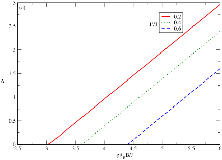
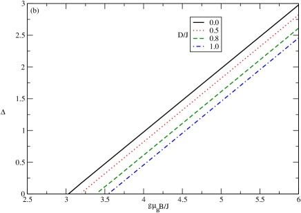
Figure 1: (a) Energy gap ($\Delta$) versus magnetic field ($g\mu_{B}B/J$) for $D/J=0.2$ and different values $J^{\prime}/J$ by setting $kT/J=0.05$. (b)Energy gap ($\Delta$) versus magnetic field ($g\mu_{B}B/J$) for $J^{\prime}/J=0.2$ and different values $D/J$ by setting $kT/J=0.05$. The change in the critical magnetic field (where the gap vanishes) for various anisotropies is remarkable.

In Fig.1(a) we have plotted the energy gap ($\Delta$) versus magnetic field $g\mu_{B}B/J$ for different values of next nearest neighbor coupling exchange constant $J^{\prime}/J$ for $D/J=0.2$ by setting $k_{B}T/J=0.05$. It is obvious from Fig.1(a) that the energy gap vanishes as the magnetic field approaches the critical value for $g\mu_{B}B_{c}/J$. For all values of $J^{\prime}/J$, the gap vanishes at the critical point $g\mu_{B}B_{c}/J$ where the transition from gapped spin liquid phase to the gapless one occurs. According to Fig.1(a), the critical field increases with $J^{\prime}/J$. For magnetic fields above critical field $g\mu_{B}B_{c}/J$, energy gap exists to the lowest excited state which is called spinon spectrum. Decreasing the magnetic field leads to vanish the energy gap and a gapless magnetic ordering state develops for magnetic fields below $g\mu_{B}B_{c}/J$ for each $J^{\prime}/J$. According to this figure the magnetic field region where excitation spectrum becomes gapless grows with anisotropy parameter. In other words the field induced spin-polarized phase sets up in lower magnetic field with decrease of $J^{\prime}/J$.

The effect of DM interaction strength, $D$, on critical magnetic field has been studied in Fig.1(b). In this figure, energy gap ($\Delta$) versus magnetic field $g\mu_{B}B/J$ for different values of Dzyaloshinskii-Moriya interaction strength $D/J$ for $J^{\prime}/J=0.2$ by setting $k_{B}T/J=0.05$ has been plotted. Fig.1(b) shows that the energy gap vanishes as the magnetic field approaches the critical value for $g\mu_{B}B_{c}/J$. For all values of $D/J$, the gap vanishes at the critical point $g\mu_{B}B_{c}/J$ where the transition from gapped spin liquid phase to the gapless one occurs. Moreover the critical field tends to higher value with increase of $D/J$ according to Fig.1(b).

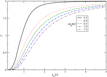
Figure 2: Magnetic specific heat as a function of $k_{B}T/J$ for different values of magnetic fields for fixed Dzyaloshinskii-Moriya interaction parameter $D/J=0.2$ and $J^{\prime}/J=0.2$.

The temperature behavior of magnetic specific heat of localized electrons on honeycomb lattice for various magnetic fields has been plotted in Fig.(2) by setting $D/J=J^{\prime}/J=0.2$. Since our approach is based on the high magnetic field limit the value of magnetic field is restricted to $B>B_{c}$ where $B_{c}$ is the critical field at finite temperature. Each curve shows an exponential decay at low temperature which manifests the presence of a finite-energy gap. Larger values of $g\mu_{B}B/J$ show more rapid decay corresponding to larger energy gap. This increasing behavior of specific heat is in agreement with experimental measurements[26]. In this study the temperature behavior of specific heat has been measured for magnetic fields above and below threshold field. Fig.(2) indicates the increase of magnetic field leads to decrease of specific heat for all temperature region. It can be understood from the fact the energy gap width grows with increase of magnetic field $g\mu_{B}B/J$. In other hand the low temperature limit of specific heat is proportional to $1/Te^{-\Delta/T}$ and therefore the decrease of specific heat with magnetic field can be justified. Since hard core bosons behave as classical objects at high temperatures, specific heat gets the constant value in this temperature region for all magnetic fields as shown in Fig.(2). Specific heat becomes constant in temperature region above characteristic temperature 2.5 for normalized magnetic field $g\mu_{B}B/J=5.5$. The increase of magnetic field leads to increase of this characteristic temperature according to Fig.(2). Similar behaviors of specific heat of localized electrons on honeycomb lattice have been obtained by numerical results. In a numerical calculations based on high temperature series expansions[27] the specific heat and susceptibility of honeycomb lattice Heisenberg model have been studied. An increasing behavior for specific heat at low temperatures has been obtained in this work. Such results for specific heat is in agreement with our results for specific heat of localized electrons on honeycomb lattice. Also in the other numerical work, temperature dependence of magnetic structure factors and specific heat of Heisenberg model on honeycomb structure has been investigated using numerical exact diagonalization method[28]. Moreover the staggered magnetization and specific of Heisenberg model Hamiltonian on honeycomb lattice has been studied by exploiting numerical quantum monte carlo method[29]. The general behaviors of temperature dependence of specific heat is in agreement with our results. The magnetic properties of the two-dimensional S = 1/2 quantum antiferromagnetic Heisenberg model on a honeycomb lattice are studied by means of a continuous Euclidean time Quantum-Monte-Carlo algorithm[30].

The effect of next nearest neighbor coupling exchange constant $J^{\prime}/J$ on the temperature behavior of specific heat at fixed magnetic field $g\mu_{B}B/J=6.0$ for $D/J=0.2$ is shown in Fig.3(a). Here $J^{\prime}$ has a direct influence on the energy gap and hence on the bosonic density as shown in Fig.3(a). The increase of $J^{\prime}/J$ raises the energy gap which gives lower specific heat at a given normalized temperature where specific heat behaves as $1/Te^{-E_{g}/T}$. Furthermore Fig.3(a) implies specific heat reaches a constant value for temperatures above a characteristic temperature. According to Fig.3(a) this characteristic temperature goes to lower value with $J^{\prime}$. This can be understood from this fact that increase of $J^{\prime}$ leads to decrease of energy gap and thus transition of bosons from ground state to excited state are performed at lower temperatures. Consequently classical behavior of bosons begins at higher temperatures with decrease of next nearest neighbor coupling exchange constant $J^{\prime}$.

In Fig.3(b), we plot specific heat versus normalized temperature for different values of DM interaction strength , namely $D/J=0.2,0.6,0.8,1.5$ for $J^{\prime}/J=0.2$ at fixed magnetic field $g\mu_{B}B/J=6.0$. This plot indicates that specific heat increases with temperature for each value of $D/J$ up to a characteristic temperature. Upon increasing temperature above characteristic one, specific heat gets a constant value. The characteristic temperature tends to lower amounts with $D/J$ as shown in Fig.3(b). This can be justified from the fact that energy gap decreases with $D$ which consequently reduces this characteristic temperature.

In Fig.4(a), we plot specific heat versus normalized magnetic field $g\mu_{B}B/J$ for different values of next nearest neighbor coupling exchange constant at fixed normalized temperature $k_{B}T/J=0.03$ for $D/J=0.2$. This plot indicates a monotonic decrease of specific heat for all values of $J^{\prime}/J$ on the whole range of magnetic field. It can be understood from the fact that energy gap grows with magnetic field and consequently thus the Bosonic density reduces. This fact leads to the decrease of the specific heat. Also Fig.4(a) shows the specific heat goes to zero at magnetic fields above 5.9 for all values of $J^{\prime}/J$. For each anisotropy parameter $\nu$, we have a different critical field, so that the hard core Bosonic representation works fine for magnetic fields above the critical field. According to Fig.4(a), specific heat increases with $J^{\prime}/J$ for fixed normalized magnetic field. This behavior arises from this point that energy gap reduces with $J^{\prime}$ which leads to increase specific heat.

Similar behavior has been obtained for DM interaction effects on magnetic field dependence of specific heat. We have plotted specific heat of Heisenberg model Hamiltonian on honeycomb lattice as a function of normalized magnetic field for different values of $D/J$ for $J^{\prime}/J=0.2$ by setting $k_{B}T/J=0.03$ in Fig.4(b). A decreasing behavior for magnetic field dependence of specific heat is clearly observed for each $D/J$ due to increase of energy gap with magnetic field. Moreover specific heat enhances with increase of DM interaction strength. This arises from this fact that energy gap reduces with $D/J$ which leads to increase of specific heat.

We have also studied the behavior of longitudinal magnetization along perpendicular to the plane for localized electrons on two dimensional honeycomb lattice described by Heisenberg model Hamiltonian. Fig.5(a) shows longitudinal magnetization ($M$) as a function of magnetic field $g\mu_{B}B/J$ for different values of $J^{\prime}/J$. For each value of $J^{\prime}/J$, $M$ increases with magnetic field. The population of bosons decreases with magnetic field and consequently magnetization increases based on Eq.(29). Upon increasing normalized magnetic field ($g\mu_{B}B/J$) above 9.0 the magnetization reaches its saturate value. All curves fall on each other in magnetic field region above 9.0 according Fig.5(a).

We have also studied the effect of DM interaction strength on the magnetic field dependence of longitudinal magnetization of the system. In Fig.5(b), we plot $M$ versus normalized magnetic field for different values of DM integration strength, namely $D/J=0.0,0.5,1.0,1.5,2.0$ for $J^{\prime}/J=0.2$ at fixed normalized temperature $k_{B}T/J=0.1$. This plot indicates the increase of magnetic field raises $M$ for all values of $D/J$ . This fact can be understood that magnetic field causes to decrease of bosonic density and therefore magnetization grows with temperature. Upon more increasing normalized magnetic field above 8.5, $M$ gets its saturate value for all values of $D/J$. At higher values of magnetic field above 8.0, the magnetization is independent of Dzyaloshinskii-Moreover interaction strength and all curves fall on each other in this magnetic field region as shown in Fig.5(b).

Finally we have studied the dependence of longitudinal magnetization on DM interaction strength for various $J^{\prime}/J$ for $g\mu_{B}B/J=6.0$ in Fig.(6). Magnetization shows no considerable dependence on $D$ in the region $D/J<1.0$ for each value of next nearest neighbor coupling exchange constant $J^{\prime}/J$. Upon more increasing $D/J$ above 1.0, the magnetization reduces. This behavior can be understood from this fact that Dzyaloshinskii-Moriya interaction leads to coupling between the transverse components of spin operators which consequently decreases the magnetic ordering along perpendicular to the plane. However the slope of the reduction increases with $J^{\prime}/J$ based on Fig.(6). Moreover the magnetization decreases with next nearest neighbor coupling exchange constant $J^{\prime}/J$ at fixed $D/J$.

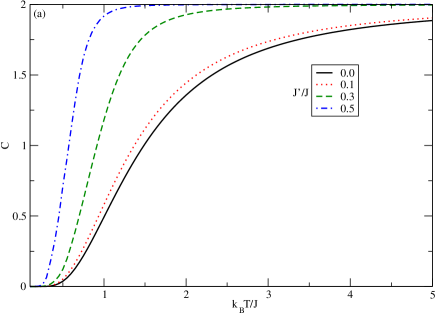
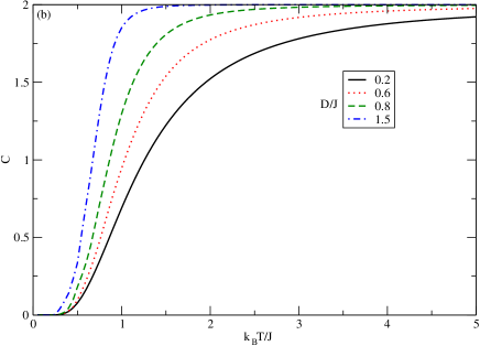
Figure 3: (a) Magnetic specific heat as a function of $k_{B}T/J$ for different values of next nearest neighbor coupling exchange constant for fixed Dzyaloshinskii-Moriya interaction parameter $D/J=0.2$. Also renormalized magnetic field is fixed at $g\mu_{B}B/J=6.0$ above threshold magnetic field. (b) Magnetic specific heat as a function of $k_{B}T/J$ for different values of Dzyaloshinskii-Moriya interaction parameter for fixed next nearest neighbor coupling exchange constant $J^{\prime}/J=0.2$ and $g\mu_{B}B/J=6.0$.

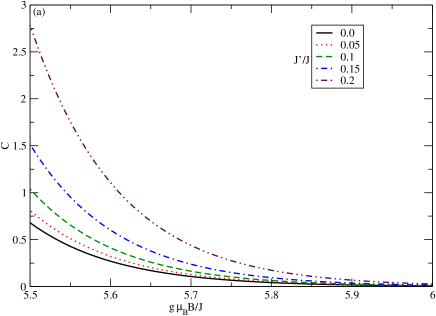
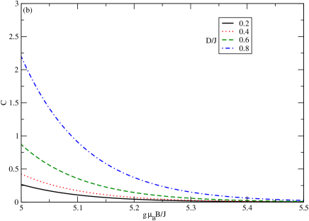
Figure 4: (a) Magnetic specific heat as a function of normalized magnetic field $g\mu_{B}B/J$ for different values of next nearest neighbor coupling exchange constant $J^{\prime}/J$ for $D/J=0.2$ and $k_{B}T/J=0.1$. (b) Magnetic specific heat as a function of normalized magnetic field $g\mu_{B}B/J$ for different values of Dzyaloshinskii-Moriya interaction parameter $D/J$ for $J^{\prime}/J=0.2$ and $k_{B}T/J=0.1$.

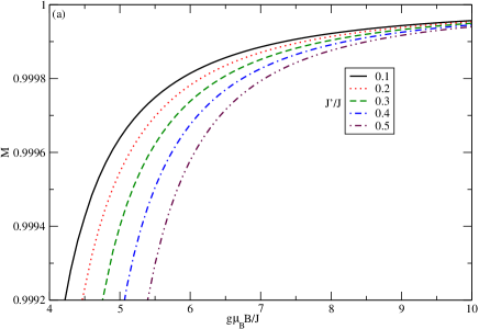
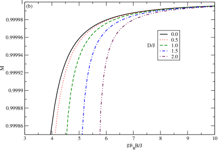
Figure 5: (a) Longitudinal magnetization as a function of normalized magnetic field $g\mu_{B}B/J$ for different values of next nearest neighbor coupling exchange constant $J^{\prime}/J$ and $D/J=0.2$ at fixed temperature and $k_{B}T/J=0.1$. (b) Longitudinal magnetization as a function of normalized magnetic field $g\mu_{B}B/J$ for different values of $D/J$ and $J^{\prime}/J=0.2$ at fixed temperature and $k_{B}T/J=0.1$.

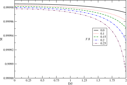
Figure 6: Longitudinal magnetization as a function of Dzyaloshinskii-Moriya interaction strength for fixed normalized magnetic field $g\mu_{B}B/J=6.0$ by setting $k_{B}T/J=0.1$.

5 Appendix: Energy Spectrum and Bogoliuobov coefficients

In this appendix we discuss the details of calculations of excitation energies and Bogoliubov coefficients $u,v$ presented in Eqs.(10,11). In the following, we will demonstrate that energy spectrum of non interacting part of model Hamiltonian in Eq.(5) are real in spite of $u_{\bf k}$ is a complex variable. The complex conjugation of unitary transformation in Eq.(9) is given by

$$\alpha^{{\dagger}}_{{\bf k}}=v_{{\bf k}}a^{{\dagger}}_{{\bf k}}+u^{*}_{{\bf k}}b^{{\dagger}}_{{\bf k}}\;\;,\;\;\beta^{{\dagger}}_{{\bf k}}=-u_{{\bf k}}a^{{\dagger}}_{{\bf k}}+v_{{\bf k}}b^{{\dagger}}_{{\bf k}},$$ (31)

we consider $v_{\bf k}$ is real variable. Using the property of unitary transformation we can write the operators $(a_{{\bf k}},b_{{\bf k}})$ in terms of ($\alpha_{{\bf k}}$,$\beta_{{\bf k}}$) as follows

$$a_{{\bf k}}=v_{{\bf k}}\alpha_{{\bf k}}-u_{{\bf k}}\beta_{{\bf k}}\;\;,\;\;b_{{\bf k}}=u^{*}_{{\bf k}}\alpha_{{\bf k}}+v_{{\bf k}}\beta_{{\bf k}},$$ (32)

By substitution of above transformation into model Hamiltonian (Eq.(5)) we can rewrite the model Hamiltonian in Eq.(5) of the manuscript in terms of operators $\alpha,\beta$ as

$$\mathcal{H}_{bil} = \sum_{\bf k}\Big{(}\mathcal{A}_{{\bf k}}(v^{2}_{\bf k}+|u_{\bf k}|^{2})+\mathcal{B}_{{\bf k}}v_{\bf k}u^{*}_{\bf k}+\mathcal{B}^{*}_{{\bf k}}v_{\bf k}u_{\bf k}\Big{)}\alpha^{{\dagger}}_{\bf k}\alpha_{\bf k}$$ (33)

$$+ \sum_{\bf k}\Big{(}\mathcal{A}_{{\bf k}}(v^{2}_{\bf k}+|u_{\bf k}|^{2})-\mathcal{B}_{{\bf k}}v_{\bf k}u^{*}_{\bf k}-\mathcal{B}^{*}_{{\bf k}}v_{\bf k}u_{\bf k}\Big{)}\beta^{{\dagger}}_{\bf k}\beta_{\bf k}$$

$$+ \sum_{\bf k}\Big{(}(\mathcal{B}_{{\bf k}}v^{2}_{\bf k}-u^{2}_{\bf k}\mathcal{B}^{*}_{{\bf k}})\alpha^{{\dagger}}_{\bf k}\beta_{\bf k}+h.c.\Big{)}.$$

In order to diagonalize bilinear part of model Hamiltonian in terms of new operators $\alpha_{\bf k}$ and $\beta_{\bf k}$, we should apply the following relation

$$\mathcal{B}_{{\bf k}}v^{2}_{\bf k}-u^{2}_{\bf k}\mathcal{B}^{*}_{{\bf k}}=0.$$ (34)

In other hand the unitary transformation of Eq.(9) in the manuscript implies

$$v^{2}_{\bf k}+|u_{\bf k}|^{2}=1.$$ (35)

Using Eqs.(34,35), we can obtain $u_{\bf k}$ and $v_{\bf k}$ as

$$u_{\bf k}=\sqrt{\frac{\mathcal{B}_{{\bf k}}}{2\mathcal{B}^{*}_{{\bf k}}}}\;\;,\;\;v_{\bf k}=\sqrt{\frac{1}{2}}.$$ (36)

According to Eq.(33), two branches of energy spectrum, i.e. $\omega_{\alpha}({\bf k})$ and $\omega_{\alpha}({\bf k})$, of bilinear part of model Hamiltonian are given by

$$\omega_{\alpha}({\bf k}) = \mathcal{A}_{{\bf k}}(v^{2}_{\bf k}+|u_{\bf k}|^{2})+\mathcal{B}_{{\bf k}}v_{\bf k}u^{*}_{\bf k}+\mathcal{B}^{*}_{{\bf k}}v_{\bf k}u_{\bf k},$$

$$\omega_{\beta}({\bf k}) = \mathcal{A}_{{\bf k}}(v^{2}_{\bf k}+|u_{\bf k}|^{2})-\mathcal{B}_{{\bf k}}v_{\bf k}u^{*}_{\bf k}-\mathcal{B}^{*}_{{\bf k}}v_{\bf k}u_{\bf k}.$$ (37)

However $u_{\bf k}$ is a complex variable, Eq.(37) implies both $\omega_{\alpha}({\bf k})$ and $\omega_{\beta}({\bf k})$ are real functions and thus Hamiltonian remains as an hermitian operator. By substitution of Eqs.(35,36) into Eq.(37), the energy spectrum of non interacting bosons takes the following relations

$$\omega_{\alpha}({\bf k}) = \mathcal{A}_{{\bf k}}+|\mathcal{B}_{{\bf k}}|\;\;,\;\;\omega_{\beta}({\bf k})=\mathcal{A}_{{\bf k}}-|\mathcal{B}_{{\bf k}}|.$$ (38)

References

- [1] L. Balent, Nature (London) 464, 199 (2010)
- [2] P. W. Anderson, Mat. Res. Bull 8, 153 (1973)
- [3] P. Fazekas and P. W. Anderson, Phil. Mag 30, 423 (1974)
- [4] S. Liang, B. Doucot and P. W. Anderson, Phys. Rev. Lett 61, 365 (1988)
- [5] S. Sachdev, Phys. Rev. B 45, 12377 (1992)
- [6] A. W. Sandvik, Phys. Rev. Lett 95, 207203 (2005)
- [7] E. Lefancoise, etal. Phys. Rev. B 94, 214416 (2016)
- [8] N. Martin, L. -P Regnault, and S. Klimko, J. Phys. Conf. Ser 340, 012012 (2012)
- [9] O. Smirnova, etal, J. Am. Chem. Soc 131, 8313 (2009)
- [10] Y. J. Yan, etal, Phys. Rev. B 85, 85102 (2012)
- [11] Z. Y. Meng, T. C. Lang, S. Wessel, F. F. Assaad, A. Muramatsu, Nature 464, 847 (2010)
- [12] S. Sorella, Y. Otsuka, S. Yunoki, Scientific Reports 2, 992 (2012)
- [13] J. B. Fouet, P. Sindzingre, and C. Lhuillier, Eur. Phys. J. B 20, 241 (2001)
- [14] M. B. Stone, D. H. Reich, C. Broholm, K. Lefmann, C. Rischel, C. P. Landee, M. M. Turnbull, Quantum critical phase in a magnetized spin -1/2 antiferromagnetic chain, Phys. Rev. Lett 91, 037205 (2003)
- [15] F. Heidrich-Meisner, A. Honecker, W. Brenig, transport in quasi one-dimensional spin-1/2 systems, Eur. Phys. J. Special topics 151, 135 (2007)
- [16] I. Affleck and M. Oshikawa, field induced gap in Cu benzoate and other spin half antiferromagnetic chains, Phys. Rev. B 60, 1038 (1999)
- [17] G. Uimim, Y. Kudasov, P. Fulde and A. Ovchinikov, Low energy excitations of Yb4As3 in a magnetic field, Euro, Phys. J. B 16, 241 (2000)
- [18] D. Dimitriev and V. Krivnov, gap genertaion in the XXZ model in transverse field, Phys. Rev. B 70, 144414 (2004)
- [19] Auerbach A 1994 Interacting electrons and Quantum Magnetism (New York: springer-Verlag Inc.)
- [20] G. D. Mahan, Many-partilce physics (Kluwer Academic/Plenum Publishers, 2000).
- [21] H. Rezania, Physica E 101, 239 (2018)
- [22] H. Rezania, Journal of Magnetism and Magnetic Materials 388, 68 (2015)
- [23] A. Abrikosov, L.Gorkov, and T. Dzyloshinskii, Methods of Quantum Field Theory in Statistical Physics (Dover, New York, 1975)
- [24] H. Rezania, A. Langari and P. Thalmeier, Phys.Rev. B 77, 094438 (2008)
- [25] A. L. Fetter and J. D. Walecka, Quantum Theory of Many Particle Systems
- [26] T. Hong, Y. H. Kim, C. Hotta, Y.Tanako, G. Tremelling, M. M. Turnbull, C. P. Landee, H. -J. Kang, N. B. Christensen, K. Lefmann, K. P. Schmidt, G. S. Uhrig, C. Broholm, Phys . Rev . Lett 105, 137207 (2010)
- [27] R. R. P. Singh and J. Oitmaa, Phys. Rev. B 96, 144414 (2017)
- [28] Y. Yamaji, T. Suzuki, T. Yamada, S-i. Suga, N. Kawashima, and M. Imada, Phys. Rev. B 93.174425 (2016)
- [29] Y. Z. Huang and G. Su, Phys. Rev. E 95, 052147(2017)
- [30] U. Low, Condensed Matter Physics 12, 497 (2009)