Existence and probabilistic representation of the solutions of semilinear parabolic PDEs with fractional Laplacians

Abstract

We obtain existence results for the solution $u$ of nonlocal semilinear parabolic PDEs on ^d with polynomial nonlinearities in $(u,\nabla u)$, using a tree-based probabilistic representation. This probabilistic representation applies to the solution of the equation itself, as well as to its partial derivatives by associating one of $d$ marks to the initial tree branch. Partial derivatives are dealt with by integration by parts and subordination of Brownian motion. Numerical illustrations are provided in examples for the fractional Laplacian in dimension up to $10$, and for the fractional Burgers equation in dimension two.

Keywords: Semilinear PDEs, nonlocal PDEs, branching processes, pseudodifferential operators, fractional Laplacian, Lévy processes, stable processes, subordination, Volterra integral equations, Monte-Carlo method.

Mathematics Subject Classification (2020): 35K58, 35K55, 35R11, 47G30, 35S05, 35B65, 35S10, 60J85, 65R20, 60G51, 60G52, 65C05, 45D05, 33C05, 60H07.

1 Introduction

Nonlocal partial differential operators such as the fractional Laplacian are useful in the modeling of anomalous diffusion phenomena driven in particular by stable Lévy processes, and they have found applications in multiple fields of engineering, physics and finance. The numerical solution of elliptic boundary value problems involving fractional Laplacians have been studied by means of finite differences in the one-dimensional case in e.g. Huang and Oberman (2016) in the parabolic case, and in Acosta et al. (2018), and Acosta and Borthagaray (2021) in the elliptic case.

Probabilistic approaches relying on the Feynman-Kac formula represent alternatives to finite differences for the numerical solution of parabolic partial differential equations. The use of stochastic diffusion branching mechanisms for the representation of solutions of partial differential equations has been introduced by Skorokhod (1964), and this construction has been extended in Ikeda et al. (1968-1969) to branching Markov processes. In Nagasawa and Sirao (1969), branching Markov processes have been applied to the blowup of solutions of a wide class of parabolic PDEs using their Duhamel integral formulations and the Markov property of the branching process at its first branching time. The branching mechanism has also been applied in McKean (1975) to the KPP equation, and to the blow-up of solutions of Fujita (1966) equations of the form $\partial u(t,x)/\partial t=\Delta u(t,x)+cu^{\beta}(t,x)$ in López-Mimbela (1996), see also Chakraborty and López-Mimbela (2008) for the existence of solutions of parabolic PDEs with power series nonlinearities. Related arguments have also been applied to Fourier-transformed PDEs in order to treat the Navier-Stokes equation by the use of stochastic cascades in Le Jan and Sznitman (1997), see also Blömker et al. (2007) for the representation of Fourier modes for the solution of class of semilinear parabolic PDEs.

This branching argument has been recently extended in Henry-Labordère et al. (2019) to the treatment polynomial non-linearities in gradient terms. For this, branches associated to gradient terms are specified using marks, and are subject to Malliavin integrations by parts. This approach applies in principle to continuous Itô diffusion generators, provided that the corresponding Malliavin weight can be successfully estimated. In the absence of gradient nonlinearities, the tree-based approach has been recently implemented for nonlocal semilinear PDEs in Belak et al. (2020).

In this paper, we obtain existence results for the solution of nonlocal semilinear PDEs by extending the above arguments from the standard Laplacian $\Delta$ to pseudo-differential operators of the form $-\eta(-\Delta/2)$, where $\eta$ is a Bernstein function such that $\eta(0^{+})=0$.

Precisely, given a horizon time $T>0$, we consider the semilinear PDE given as

$$\begin{cases}\displaystyle\frac{\partial u}{\partial t}(t,x)-\eta(-\Delta/2)u(t,x)+f\left(t,x,u(t,x),\frac{\partial u}{\partial x_{1}}(t,x),\ldots,\frac{\partial u}{\partial x_{m}}(t,x)\right)=0,\vskip 6.0pt plus 2.0pt minus 2.0pt\\ u(T,x)=\phi(x),\qquad x=(x_{1},\ldots,x_{d})\in{}^{d},\end{cases}$$ (1.1)

where $f(t,x,y,z_{1},\ldots,z_{m})$ is a polynomial nonlinearity given by

$$f(t,x,y,z_{1},\ldots,z_{m})=\sum\limits_{l=(l_{0},\ldots,l_{m})\in{\cal L}_{m}}c_{l}(t,x)y^{l_{0}}z^{l_{1}}_{1}\cdots z^{l_{m}}_{m},$$

$t\in{}_{+}$, $x,y,z_{1},\ldots,z_{m}\in\real$, for some $m\in\{0,\ldots,d\}$, where ${\cal L}_{m}$ is a finite subset of $\mathbb{N}^{m+1}$ and $c_{l}(t,x)$ are measurable functions of $(t,x)\in[0,T]\times{}^{d}$, $l=(l_{0},\ldots,l_{m})\in{\cal L}_{m}$. In the sequel, we let $\|x\|:=\sqrt{x_{1}^{2}+\cdots+x_{d}^{2}}$, $x=(x_{1},\ldots,x_{d})\in{}^{d}$.
Assumption ($A$): We assume that the coefficients $c_{l}(t,x)$ are uniformly bounded, i.e.

$$|c_{l}|_{\infty}:=\sup_{t\in[0,T],x\in\mathbb{R}^{d}}|c_{l}(t,x)|<\infty,\qquad l=(l_{0},\ldots,l_{m})\in{\cal L}_{m},$$ (1.2)

and that the terminal condition $\phi$ is Lipschitz, i.e.

$$|\phi(x)-\phi(y)|\leq L\|x-y\|,\qquad x,y\in{}^{d},$$ (1.3)

for some $L>0$, and bounded on ^d.

In the sequel, we will say that a function $u(t,x)$ is an integral solution if $u(t,x)$ satisfies the Duhamel formulation of (1.1), i.e.

$$u(t,x) = \int_{{}^{d}}\varphi(T-t,y-x)\phi(y)dy$$

$$+\sum_{l=(l_{0},\ldots,l_{m})\in{\cal L}_{m}}\int_{t}^{T}\int_{{}^{d}}\varphi(s-t,y-x)c_{l}(s,y)u^{l_{0}}(s,y)\prod_{j=1}^{m}\left(\frac{\partial u}{\partial y_{j}}(s,y)\right)^{l_{j}}dyds,$$

$(t,x)\in[0,T]\times{}^{d}$. Note that the above setting includes the case of the standard fractional Laplacian $\Delta_{\alpha}=-\eta(-\Delta/2)$ by choosing the Laplace exponent $\eta(\lambda)=(2\lambda)^{\alpha/2}$.

In particular, in Theorem 3.1 we provide probabilistic representations for the solutions of a wide class of semilinear parabolic PDEs of the form

$$\frac{\partial u}{\partial t}(t,x)-\eta(-\Delta/2)u(t,x)+f\left(t,x,u(t,x),\frac{\partial u}{\partial x_{1}}(t,x),\ldots,\frac{\partial u}{\partial x_{m}}(t,x)\right)=0,~{}~{}u(T,\cdot)=\phi(\cdot),$$ (1.5)

$(t,x)\in[0,T]\times\mathbb{R}^{d}$, with polynomial non-linearity $f$ in the solution $u$ and its partial derivatives $\partial u/\partial x_{i}$, $i=1,\ldots,m$, and $\eta$ is a Bernstein function that satisfies $\eta(0^{+})=0$.

The probabilistic representations of Theorem 3.1 uses a functional of a random branching process driven by a subordinated Lévy process $(Z_{t})_{t\in{}_{+}}:=(B_{S_{t}})_{t\in{}_{+}}$, where $(B_{t})_{t\in{}_{+}}$ is a standard $d$-dimensional Brownian motion and $(S_{t})_{t\in{}_{+}}$ is a Lévy subordinator with Laplace exponent $\eta$ such that

$$\mathbb{E}\big{[}e^{-\lambda S_{t}}\big{]}=e^{-t\eta(\lambda)},\qquad\lambda,t\geq 0,$$

see e.g. Theorem 1.3.23 and pages 55-56 in Applebaum (2009). Then, by Proposition 1.3.27 in Applebaum (2009), $(Z_{t})_{t\in{}_{+}}$ has Lévy symbol $\psi_{Z}(\xi)=-\eta(\|\xi\|^{2}/2)$ such that $\mathbb{E}\big{[}e^{i\xi Z_{t}}\big{]}=e^{t\psi_{Z}(\xi)}$, $\xi\in{}^{d}$, $t\geq 0$, and, by Theorem 3.3.3 therein, the infinitesimal generator of $(Z_{t})_{t\in{}_{+}}$ is the pseudo-differential operator $-\eta(-\Delta/2)$.

In the case of stable processes we have $\eta(\lambda):=(2\lambda)^{\alpha/2}$, and $-\eta(-\Delta/2)$ becomes the fractional Laplacian

$$\Delta_{\alpha}u=-(-\Delta)^{\alpha/2}u=\frac{2^{\alpha}\Gamma(d/2+\alpha/2)}{\pi^{d/2}|\Gamma(-\alpha/2)|}\lim_{r\rightarrow 0^{+}}\int_{\mathbb{R}^{d}\backslash B(x,r)}\frac{u(\cdot+z)-u(z)}{|z|^{d+\alpha}}dz,$$

for $\alpha\in(0,2]$, where $\Gamma(p):=\displaystyle\int_{0}^{\infty}e^{-\lambda x}\lambda^{p-1}d\lambda$, $p>0$, is the gamma function, see e.g. Kwaśnicki (2017).

For each $i=0,1,\ldots,d$ we construct a sufficiently integrable functional $\mathcal{H}_{\phi}(\mathcal{T}_{t,x,i})$ of a random tree $\mathcal{T}_{t,x,i}$ such that we have the representations

$$u(t,x):=\mathbb{E}\big{[}\mathcal{H}_{\phi}(\mathcal{T}_{t,x,0})\big{]},\quad(t,x)\in[0,T]\times{}^{d},$$

and

$$\frac{\partial u}{\partial x_{i}}(t,x):=\mathbb{E}\big{[}\mathcal{H}_{\phi}(\mathcal{T}_{t,x,i})\big{]},\quad(t,x)\in[0,T]\times{}^{d},\quad i=1,\ldots,d,$$

see Theorem 3.1. Dealing with gradient terms in the proof of Theorem 3.1 requires to perform an integration by parts, which is made possible using the Gaussian density of $B_{t}$ in the subordination $Z_{t}:=B_{S_{t}}$, as done in Kawai and Takeuchi (2013) in the case of stable processes with $\eta(\lambda):=(2\lambda)^{\alpha/2}$.

As a consequence of Theorem 3.1, in Proposition 3.2 we show that the probabilistic representation of Theorem 3.1 can be used to recover the classical result of Fujita (1966) on the blow-up of semilinear PDEs.

While the branching tree mechanism is quite general and can be applied to a wide range of differential equations via formal calculations, proving the existence of solutions requires to show the integrability of functional $\mathcal{H}_{\phi}(\mathcal{T}_{t,x,i})$ representing the PDE solution $u(t,x)$ and its partial derivatives. We deal with this integrability using existence results for the solutions of Volterra integral equations, instead of using ODEs as in e.g. Henry-Labordère and Touzi (2018) and Henry-Labordère et al. (2019).

Theorem 4.1, we show that the integrability required for the probabilistic representation Theorem 3.1 is satisfied provided that $\lambda\rightarrow 1/(\sqrt{\lambda}\eta(\lambda))$ is integrable at $+\infty$. In comparison with recent work in the diffusion case, see Henry-Labordère et al. (2019), our integrability condition (3.2)-(3.3) in Theorem 3.1 is sharper because it only involves mark indexes of partial derivatives appearing in the main PDE. In addition, we provide a detailed justification for the commutation relation (3.7) instead of stating it as an assumption as in Henry-Labordère et al. (2019), see Assumption 3.2 therein.

As a direct consequence of Theorems 3.1 and 4.1, we obtain the following result on local-in-time existence of solutions.

Theorem 1.1

Under Assumption ($A$), suppose that

$$\int_{\lambda_{0}}^{\infty}\frac{1}{\sqrt{\lambda}\eta(\lambda)}d\lambda<\infty$$

for some $\lambda_{0}>0$. Then, there exists a small enough $T>0$ such that the PDE (1.1) admits an integral solution on $[0,T]$ in the sense of (1).

Related local and global-in-time existence results have been obtained for generalized fractional Laplacians by deterministic arguments under more technical conditions in e.g. Ishige et al. (2014) and more recently in Ishige et al. (2021) for power nonlinearities of sufficiently low orders. In the particular case of the $\alpha$-fractional Laplacian where $\eta(\lambda):=(2\lambda)^{\alpha/2}$ with $\alpha\in(1,2)$, we obtain the following corollary.

Corollary 1.2

Taking $\eta(\lambda):=(2\lambda)^{\alpha/2}$ with $\alpha\in(1,2)$, under Assumption ($A$) there exists a small enough $T>0$ such that the PDE (1.1) with $\alpha$-fractional Laplacian admits an integral solution on $[0,T]$ in the sense of (1).

In the case of the fractional Laplacian, Proposition 4.4 provides quantitative estimates on the horizon time $T$, ensuring existence of solutions on $[0,T]$ by Theorem 3.1.

We also provide a Monte Carlo implementation of our algorithm for the numerical solutions of nonlinear fractional PDEs with and without gradient term in dimension up to 10, and of a fractional Burgers equation. The tree-based Monte Carlo method avoids the curse of dimensionality, whereas the application of deterministic numerical methods is notoriously difficult including in the fractional case, see, e.g., Bonito et al. (2018).

The paper is organized as follows. In Section 2 we present the description of the branching mechanism in Section 2. In Section 3 we state our main result Theorem 3.1 which gives the probabilistic representation of the solution and its partial derivatives. In Section 4 we give give a sufficient condition on the Bernstein function $\eta$ that ensures the integrability needed for the the probabilistic representation of Theorem 3.1 to hold. In Section 5, we present some numerical simulations to illustrate the method on specific examples.

Bernstein functions and subordinators

Let $\eta:(0,\infty)\rightarrow[0,\infty)$ denote a Bernstein function, i.e. $\eta$ is a $C^{\infty}$ function whose $nth$ derivative satisfies $(-1)^{n}\eta^{(n)}\leq 0$ for all $n\geq 1$, and $\lim_{z\searrow 0}\eta(z)=0$, see Theorem 1.3.23 in Applebaum (2009). We consider a subordinator $(S_{t})_{t\in{}_{+}}$, i.e. a ₊-valued non-decreasing Lévy process, with Laplace exponent $\eta$, which admits the representation

$$\eta(\lambda)=b\lambda+\int_{0}^{\infty}(1-e^{-\lambda y})\nu(dy),$$ (1.6)

where $b\geq 0$ and the Lévy measure $\nu$ satisfies

$$\int_{0}^{\infty}(y\wedge 1)\nu(dy)<\infty,$$

see Theorem 1.3.15 in Applebaum (2009). Using the identity

$$x^{-p}=\frac{1}{\Gamma(p)}\int_{0}^{\infty}e^{-\lambda x}\lambda^{p-1}d\lambda\qquad x>0,$$ (1.7)

the negative moments of $S_{t}$ are given by

$$\mathbb{E}\big{[}S_{t}^{-p}\big{]}=\frac{1}{\Gamma(p)}\int_{0}^{\infty}e^{-t\eta(\lambda)}\lambda^{p-1}d\lambda,\qquad p>0.$$ (1.8)

When $(S_{t})_{t\in{}_{+}}$ is an $\alpha/2$-stable subordinator with Laplace exponent $\eta(\lambda)=(2\lambda)^{\alpha/2}$, the subordinated process $Z_{t}=B_{S_{t}}$ becomes an $\alpha$-stable process with generator $\Delta_{\alpha}$. In that case, we have $b=0$ in (1.6), the Lévy measure $\nu$ of the subordinator $(S_{t})_{t\in{}_{+}}$ is given by

$$\nu(dx)=\alpha\frac{2^{\alpha/2-1}}{\Gamma(1-\alpha/2)}\frac{dx}{x^{1+\alpha/2}},$$

and its Lévy symbol $\psi_{S}$ satisfies

$$\psi_{S}(\xi) = \frac{2^{\alpha/2}\alpha}{2\Gamma(1-\alpha/2)}\int_{0}^{\infty}(e^{i\xi y}-1)\frac{dy}{y^{1+\alpha/2}}$$ (1.9)

$$= \frac{\alpha(2|\xi|)^{\alpha/2}}{2\Gamma(1-\alpha/2)}\Gamma(-\alpha/2)e^{i\alpha\arg(-i\xi)/2}$$

$$= -\cos\left(\frac{\pi\alpha}{4}\right)(2|\xi|)^{\alpha/2}\left(1-i\ \!\mathrm{sign}\>(\xi)\tan\left(\frac{\pi\alpha}{4}\right)\right),\qquad\xi\in\real,$$

where we used the identity

$$\int_{0}^{\infty}(e^{wy}-1)y^{-1-\alpha/2}dy=\Gamma(-\alpha/2)|w|^{\alpha/2}e^{i\alpha\arg(-w)/2}$$

which is valid for $\alpha\in(0,2)$ and any $w\in\mathbb{C}^{*}$ with $\eufrak{R}(w)\leq 0$, see Relation (14.18) page 84 of Sato (1999). In this case, the negative moments of $S_{t}$ are given by

$$\mathbb{E}\big{[}S_{t}^{-p}\big{]} = \frac{1}{\Gamma(p)}\int_{0}^{\infty}e^{-t(2\lambda)^{\alpha/2}}\lambda^{p-1}d\lambda$$ (1.10)

$$= \frac{1}{t^{2p/\alpha}}\frac{2^{1-p}}{\alpha\Gamma(p)}\int_{0}^{\infty}u^{-1+2p/\alpha}e^{-u}du$$

$$= \frac{2^{1-p}\Gamma(2p/\alpha)}{\alpha t^{2p/\alpha}\Gamma(p)},\qquad p>0.$$

2 Random trees with marked branches

In the sequel, we will provide a probabilistic representation for the solution of (1.1), using a branching mechanism such that the solution of (1.1) will be given by the expectation of a multiplicative functional defined on a random tree structure.

Let $\rho:\mathbb{R}^{+}\rightarrow(0,\infty)$ be a probability density function on ₊, and consider a probability mass function $(q_{l_{0},\ldots,l_{m}})_{(l_{0},\ldots,l_{m})\in{\cal L}_{m}}$ on ${\cal L}_{m}$ with $q_{l_{0},\ldots,l_{m}}>0$, $(l_{0},\ldots,l_{m})\in{\cal L}_{m}$, and $\sum_{(l_{0},\ldots,l_{m})\in{\cal L}_{m}}|l|q_{l_{0},\ldots,l_{m}}<\infty$, where $|l|=l_{0}+\cdots+l_{m}$. In addition, we consider

• an i.i.d. family $(\tau^{i,j})_{i,j\geq 1}$ of random variables with distribution $\rho(t)dt$ on ₊,

• an i.i.d. family $(I^{i,j})_{i,j\geq 1}$ of discrete random variables, with

  $$\mathbb{P}\big{(}I^{i,j}=(l_{0},\ldots,l_{m})\big{)}=q_{l_{0},\ldots,l_{m}}>0,\qquad(l_{0},\ldots,l_{m})\in{\cal L}_{m},$$ (2.1)

• an independent family $(Z^{i,j})_{i,j\geq 1}$ of subordinated Lévy processes constructed as

  $$Z^{i,j}_{t}:=B^{i,j}_{S^{i,j}_{t}},\qquad t\in{}_{+},\quad i,j\geq 1,$$

  where $(B^{i,j})_{i,j\geq 1}$ and $(S^{i,j})_{i,j\geq 1}$ are independent standard Brownian motions and independent subordinators with Laplace exponent $\eta$.

The sequences $(\tau^{i,j})_{i,j\geq 1}$, $(I^{i,j})_{i,j\geq 1}$ and $(Z^{i,j})_{i,j\geq 1}$ are assumed to be mutually independent.

Marked branching process

We consider a marked branching process starting from a particle at the position $x\in{}^{d}$, with label $\macc@depth\char 1\relax\frozen@everymath{\macc@group}\macc@set@skewchar\macc@nested@a 111{1}=(1)$ and mark $i\in\{0,1,\ldots,d\}$ at time $t\in[0,T]$, which evolves according to the process $X_{s,x}^{\macc@depth\char 1\relax\frozen@everymath{\macc@group}\macc@set@skewchar\macc@nested@a 111{1}}=x+Z_{s-t}^{1,1}$, $s\in[t,t+\tau^{1,1}]$.

If $\tau^{1,1}<T-t$, the process branches at time $t+\tau^{1,1}$ into new independent copies of $(Z_{t})_{t\in{}_{+}}$, each of them started at the position $X_{t+\tau^{1,1}}$ at time $t+\tau^{1,1}$. Based on the values of $I^{1,1}=(l_{0},\ldots,l_{m})\in{\cal L}_{m}$, a family of $|l|:=l_{0}+\cdots+l_{m}$ of new branches carrying respectively the marks $i=0,\ldots,d$ are created with the probability $q_{l_{0},\ldots,l_{m}}$, where

• the first $l_{0}$ branches carry the mark $0$ and are indexed by $(1,1),(1,2),\ldots,(1,l_{0})$,

• the next $l_{1}$ branches carry the mark $1$ and are indexed by $(1,l_{0}+1),\ldots,(1,l_{0}+l_{1})$, and so on.

Each new particle then follows independently the same mechanism as the first one, and every branch stops when it reaches the horizon time $T$. Particles at the generation $n\geq 1$ are assigned a label of the form $\macc@depth\char 1\relax\frozen@everymath{\macc@group}\macc@set@skewchar\macc@nested@a 111{k}=(1,k_{2},\ldots,k_{n})\in\mathbb{N}^{n}$, and their parent is labeled $\macc@depth\char 1\relax\frozen@everymath{\macc@group}\macc@set@skewchar\macc@nested@a 111{k}-:=(1,k_{2},\ldots,k_{n-1})$. The particle labeled $\macc@depth\char 1\relax\frozen@everymath{\macc@group}\macc@set@skewchar\macc@nested@a 111{k}$ is born at time $T_{\macc@depth\char 1\relax\frozen@everymath{\macc@group}\macc@set@skewchar\macc@nested@a 111{k}-}$ and its lifetime $\tau^{n,\pi_{n}(\macc@depth\char 1\relax\frozen@everymath{\macc@group}\macc@set@skewchar\macc@nested@a 111{k})}$ is the element of index $\pi_{n}(\macc@depth\char 1\relax\frozen@everymath{\macc@group}\macc@set@skewchar\macc@nested@a 111{k})$ in the i.i.d. sequence $(\tau^{n,j})_{j\geq 1}$, defining a random injection

$$\pi_{n}:\mathbb{N}^{n}\to\mathbb{N},\qquad n\geq 1.$$

The random evolution of particle $\macc@depth\char 1\relax\frozen@everymath{\macc@group}\macc@set@skewchar\macc@nested@a 111{k}$ is given by

$$X_{s,x}^{\macc@depth\char 1\relax\frozen@everymath{\macc@group}\macc@set@skewchar\macc@nested@a 111{k}}:=X^{\macc@depth\char 1\relax\frozen@everymath{\macc@group}\macc@set@skewchar\macc@nested@a 111{k}-}_{T_{\macc@depth\char 1\relax\frozen@everymath{\macc@group}\macc@set@skewchar\macc@nested@a 111{k}-},x}+Z_{s-T_{\macc@depth\char 1\relax\frozen@everymath{\macc@group}\macc@set@skewchar\macc@nested@a 111{k}-}}^{n,\pi_{n}(\macc@depth\char 1\relax\frozen@everymath{\macc@group}\macc@set@skewchar\macc@nested@a 111{k})},\qquad s\in[T_{\macc@depth\char 1\relax\frozen@everymath{\macc@group}\macc@set@skewchar\macc@nested@a 111{k}-},T_{\macc@depth\char 1\relax\frozen@everymath{\macc@group}\macc@set@skewchar\macc@nested@a 111{k}}],$$ (2.2)

where $T_{\macc@depth\char 1\relax\frozen@everymath{\macc@group}\macc@set@skewchar\macc@nested@a 111{k}}:={\mathrm{{\rm T}}}_{\macc@depth\char 1\relax\frozen@everymath{\macc@group}\macc@set@skewchar\macc@nested@a 111{k}-}+\tau^{n,\pi_{n}(\macc@depth\char 1\relax\frozen@everymath{\macc@group}\macc@set@skewchar\macc@nested@a 111{k})}$.

If $T_{\macc@depth\char 1\relax\frozen@everymath{\macc@group}\macc@set@skewchar\macc@nested@a 111{k}}:={\mathrm{{\rm T}}}_{\macc@depth\char 1\relax\frozen@everymath{\macc@group}\macc@set@skewchar\macc@nested@a 111{k}-}+\tau^{n,\pi_{n}(\macc@depth\char 1\relax\frozen@everymath{\macc@group}\macc@set@skewchar\macc@nested@a 111{k})}<T$, we draw a sample $I_{\macc@depth\char 1\relax\frozen@everymath{\macc@group}\macc@set@skewchar\macc@nested@a 111{k}}:=I^{n,\pi_{n}(\macc@depth\char 1\relax\frozen@everymath{\macc@group}\macc@set@skewchar\macc@nested@a 111{k})}=(l_{0},\ldots,l_{m})$ of $I^{n,\pi_{n}(\macc@depth\char 1\relax\frozen@everymath{\macc@group}\macc@set@skewchar\macc@nested@a 111{k})}$ with distribution (2.1), and the particle $\macc@depth\char 1\relax\frozen@everymath{\macc@group}\macc@set@skewchar\macc@nested@a 111{k}$ branches into $|I^{n,\pi_{n}(\macc@depth\char 1\relax\frozen@everymath{\macc@group}\macc@set@skewchar\macc@nested@a 111{k})}|=l_{0}+\cdots+l_{m}$ offsprings at generation $(n+1)$, which are indexed by $(1,\ldots,k_{n},i)$, $i=1,\ldots,|I^{n,\pi_{n}(\macc@depth\char 1\relax\frozen@everymath{\macc@group}\macc@set@skewchar\macc@nested@a 111{k})}|$. The particles whose index ends with an integer between $1$ and $l_{0}$ will carry the mark $0$, and those with index ending with an integer between $l_{0}+\cdots+l_{i-1}+1$ and $l_{0}+\cdots+l_{i}$ will carry a mark $i\in\{1,\ldots,d\}$. Finally, the mark of particle $\macc@depth\char 1\relax\frozen@everymath{\macc@group}\macc@set@skewchar\macc@nested@a 111{k}$ will be denoted by $\theta_{\macc@depth\char 1\relax\frozen@everymath{\macc@group}\macc@set@skewchar\macc@nested@a 111{k}}\in\{0,1,\ldots,d\}$. Note that the indexes are only be used to distinguish the particles in the branching process, and they are distinct from the marks.

The set of particles dying before time $T$ is denoted by $\mathcal{K}^{\circ}$, whereas those dying after $T$ form a set denoted by $\mathcal{K}^{\partial}$.

Definition 2.1

When started at time $t\in[0,T]$ from a position $x\in{}^{d}$ and a mark $i\in\{0,1,\ldots,d\}$ on its first branch, the above construction yields a marked branching process called a random marked tree, and denoted by $\mathcal{T}_{t,x,i}$.

The tree $\mathcal{T}_{t,x,0}$ will be used for the stochastic representation of the solution $u$ of the PDE (1.1), while the trees $\mathcal{T}_{t,x,i}$ will be used for the stochastic representation of the partial derivatives $\partial u/\partial x_{i}$, $i=1,\ldots,m$. The next table summarizes the notation introduced so far.

Object	Notation
Initial time	$t$
Initial position	$x$
Tree rooted at $(t,x)$ with initial mark $i$	$\mathcal{T}_{t,x,i}$
Particle (or label) of generation $n\geq 1$	$\stackrel{{\scriptstyle}}{{\macc@depth\char 1\relax\frozen@everymath{\macc@group}\macc@set@skewchar\macc@nested@a 111{k}=(1,k_{2},\ldots,k_{n})}}$
First branching time	$T_{\macc@depth\char 1\relax\frozen@everymath{\macc@group}\macc@set@skewchar\macc@nested@a 111{1}}$
Lifespan of a particle	$\tau_{\macc@depth\char 1\relax\frozen@everymath{\macc@group}\macc@set@skewchar\macc@nested@a 111{k}}=T_{\macc@depth\char 1\relax\frozen@everymath{\macc@group}\macc@set@skewchar\macc@nested@a 111{k}}-T_{\macc@depth\char 1\relax\frozen@everymath{\macc@group}\macc@set@skewchar\macc@nested@a 111{k}-}$
Birth time of a particle $\bar{k}$	$T_{\macc@depth\char 1\relax\frozen@everymath{\macc@group}\macc@set@skewchar\macc@nested@a 111{k}-}$
Death time of a particle $\bar{k}$	$T_{\macc@depth\char 1\relax\frozen@everymath{\macc@group}\macc@set@skewchar\macc@nested@a 111{k}}$
Position at birth	$X^{\macc@depth\char 1\relax\frozen@everymath{\macc@group}\macc@set@skewchar\macc@nested@a 111{k}}_{T_{\macc@depth\char 1\relax\frozen@everymath{\macc@group}\macc@set@skewchar\macc@nested@a 111{k}-},x}$
Position at death	$X^{\macc@depth\char 1\relax\frozen@everymath{\macc@group}\macc@set@skewchar\macc@nested@a 111{k}}_{T_{\macc@depth\char 1\relax\frozen@everymath{\macc@group}\macc@set@skewchar\macc@nested@a 111{k}},x}$
Mark	$\theta_{\macc@depth\char 1\relax\frozen@everymath{\macc@group}\macc@set@skewchar\macc@nested@a 111{k}}$

To represent the structure of the tree we use the following conventions, in which different colors mean different ways of branching:

Specifically, let us draw a tree sample for the following PDE:

$$\frac{\partial u}{\partial t}-\eta(-\Delta/2)u+c_{0}(t,x)+c_{0,1}(t,x)u\frac{\partial u}{\partial x_{1}}=0$$

in dimension $d=1$. For this tree, there are two types of branching: we can either branch into no branch at all (which is represented in blue), or into two branches (one bearing the mark $0$ and one bearing the mark $1$, which is represented in purple). The black color is used for leaves that have reached the horizon time $T$.

In the above example we have $\mathcal{K}^{\circ}=\{\bar{1},(1,1),(1,2),(1,2,2)\}$ and $\mathcal{K}^{\partial}=\{(1,2,1)\}$.

3 Probabilistic representation

Given $t\in[0,T]$, $x\in\mathbb{R}^{d}$ and a mark $i\in\{0,1,\ldots,d\}$, we consider the functional $\mathcal{H}_{\phi}$ of the random tree $\mathcal{T}_{t,x,i}$, defined as

$${\mathcal{H}_{\phi}(\mathcal{T}_{t,x,i}):=\prod_{\macc@depth\char 1\relax\frozen@everymath{\macc@group}\macc@set@skewchar\macc@nested@a 111{k}\in\mathcal{K}^{\circ}}\frac{c_{I_{\macc@depth\char 1\relax\frozen@everymath{\macc@group}\macc@set@skewchar\macc@nested@a 111{k}}}\big{(}T_{\macc@depth\char 1\relax\frozen@everymath{\macc@group}\macc@set@skewchar\macc@nested@a 111{k}},X^{\macc@depth\char 1\relax\frozen@everymath{\macc@group}\macc@set@skewchar\macc@nested@a 111{k}}_{T_{\macc@depth\char 1\relax\frozen@everymath{\macc@group}\macc@set@skewchar\macc@nested@a 111{k}},x}\big{)}\mathcal{W}_{\macc@depth\char 1\relax\frozen@everymath{\macc@group}\macc@set@skewchar\macc@nested@a 111{k}}}{q_{I_{\macc@depth\char 1\relax\frozen@everymath{\macc@group}\macc@set@skewchar\macc@nested@a 111{k}}}\rho(\tau_{\macc@depth\char 1\relax\frozen@everymath{\macc@group}\macc@set@skewchar\macc@nested@a 111{k}})}\prod_{\macc@depth\char 1\relax\frozen@everymath{\macc@group}\macc@set@skewchar\macc@nested@a 111{k}\in\mathcal{K}^{\partial}}\frac{\big{(}\phi\big{(}X^{\macc@depth\char 1\relax\frozen@everymath{\macc@group}\macc@set@skewchar\macc@nested@a 111{k}}_{T,x}\big{)}-\phi\big{(}X^{\macc@depth\char 1\relax\frozen@everymath{\macc@group}\macc@set@skewchar\macc@nested@a 111{k}}_{T_{\macc@depth\char 1\relax\frozen@everymath{\macc@group}\macc@set@skewchar\macc@nested@a 111{k}-},x}\big{)}{\mathbbm{1}_{\{\theta_{\macc@depth\char 1\relax\frozen@everymath{\macc@group}\macc@set@skewchar\macc@nested@a 111{k}}\neq 0\}}}\big{)}\mathcal{W}_{\macc@depth\char 1\relax\frozen@everymath{\macc@group}\macc@set@skewchar\macc@nested@a 111{k}}}{\macc@depth\char 1\relax\frozen@everymath{\macc@group}\macc@set@skewchar\macc@nested@a 111{F}(T-T_{\macc@depth\char 1\relax\frozen@everymath{\macc@group}\macc@set@skewchar\macc@nested@a 111{k}-})}},$$

where $\macc@depth\char 1\relax\frozen@everymath{\macc@group}\macc@set@skewchar\macc@nested@a 111{F}(z):=1-\mathbb{P}(T_{\macc@depth\char 1\relax\frozen@everymath{\macc@group}\macc@set@skewchar\macc@nested@a 111{1}}\leq z)$, $z\geq 0$, and $\mathcal{W}_{\macc@depth\char 1\relax\frozen@everymath{\macc@group}\macc@set@skewchar\macc@nested@a 111{k}}$ is a random weight defined by

$$\displaystyle\mathbbm{1}_{\{\theta_{\macc@depth\char 1\relax\frozen@everymath{\macc@group}\macc@set@skewchar\macc@nested@a 111{k}}=0\}}+\mathbbm{1}_{\{\theta_{\macc@depth\char 1\relax\frozen@everymath{\macc@group}\macc@set@skewchar\macc@nested@a 111{k}}\neq 0\}}\frac{\big{(}X^{\macc@depth\char 1\relax\frozen@everymath{\macc@group}\macc@set@skewchar\macc@nested@a 111{k}}_{T_{\macc@depth\char 1\relax\frozen@everymath{\macc@group}\macc@set@skewchar\macc@nested@a 111{k}},x}-X^{\macc@depth\char 1\relax\frozen@everymath{\macc@group}\macc@set@skewchar\macc@nested@a 111{k}}_{T_{\macc@depth\char 1\relax\frozen@everymath{\macc@group}\macc@set@skewchar\macc@nested@a 111{k}-},x}\big{)}_{\theta_{\macc@depth\char 1\relax\frozen@everymath{\macc@group}\macc@set@skewchar\macc@nested@a 111{k}}}}{S^{\macc@depth\char 1\relax\frozen@everymath{\macc@group}\macc@set@skewchar\macc@nested@a 111{k}}_{T_{\macc@depth\char 1\relax\frozen@everymath{\macc@group}\macc@set@skewchar\macc@nested@a 111{k}}}-S^{\macc@depth\char 1\relax\frozen@everymath{\macc@group}\macc@set@skewchar\macc@nested@a 111{k}}_{T_{\macc@depth\char 1\relax\frozen@everymath{\macc@group}\macc@set@skewchar\macc@nested@a 111{k}-}}} \mbox{if~{}}~{}\macc@depth\char 1\relax\frozen@everymath{\macc@group}\macc@set@skewchar\macc@nested@a 111{k}\in\mathcal{K}^{\circ},$$ (3.1a)

$$\displaystyle\mathbbm{1}_{\{\theta_{\macc@depth\char 1\relax\frozen@everymath{\macc@group}\macc@set@skewchar\macc@nested@a 111{k}}=0\}}+\mathbbm{1}_{\{\theta_{\macc@depth\char 1\relax\frozen@everymath{\macc@group}\macc@set@skewchar\macc@nested@a 111{k}}\neq 0\}}\frac{\big{(}X^{\macc@depth\char 1\relax\frozen@everymath{\macc@group}\macc@set@skewchar\macc@nested@a 111{k}}_{T,x}-X^{\macc@depth\char 1\relax\frozen@everymath{\macc@group}\macc@set@skewchar\macc@nested@a 111{k}}_{T_{\macc@depth\char 1\relax\frozen@everymath{\macc@group}\macc@set@skewchar\macc@nested@a 111{k}-},x}\big{)}_{\theta_{\macc@depth\char 1\relax\frozen@everymath{\macc@group}\macc@set@skewchar\macc@nested@a 111{k}}}}{S^{\macc@depth\char 1\relax\frozen@everymath{\macc@group}\macc@set@skewchar\macc@nested@a 111{k}}_{T}-S^{\macc@depth\char 1\relax\frozen@everymath{\macc@group}\macc@set@skewchar\macc@nested@a 111{k}}_{T_{\macc@depth\char 1\relax\frozen@everymath{\macc@group}\macc@set@skewchar\macc@nested@a 111{k}-}}} \mbox{if~{}}~{}\macc@depth\char 1\relax\frozen@everymath{\macc@group}\macc@set@skewchar\macc@nested@a 111{k}\in\mathcal{K}^{\partial},$$ (3.1b)

where $\theta_{\macc@depth\char 1\relax\frozen@everymath{\macc@group}\macc@set@skewchar\macc@nested@a 111{k}}\in\{0,1,\ldots,d\}$ denotes the mark of the particle $\macc@depth\char 1\relax\frozen@everymath{\macc@group}\macc@set@skewchar\macc@nested@a 111{k}$, and for each particle labeled $\macc@depth\char 1\relax\frozen@everymath{\macc@group}\macc@set@skewchar\macc@nested@a 111{k}=(1,k_{2},\ldots,k_{n})\in\mathbb{N}^{n}$ at generation $n\geq 1$, the subordinator $\big{(}S_{t}^{\macc@depth\char 1\relax\frozen@everymath{\macc@group}\macc@set@skewchar\macc@nested@a 111{k}}\big{)}_{t\in[T_{\macc@depth\char 1\relax\frozen@everymath{\macc@group}\macc@set@skewchar\macc@nested@a 111{k}-},T_{\macc@depth\char 1\relax\frozen@everymath{\macc@group}\macc@set@skewchar\macc@nested@a 111{k}}]}$ is defined as

$$S_{t}^{\macc@depth\char 1\relax\frozen@everymath{\macc@group}\macc@set@skewchar\macc@nested@a 111{k}}:=S_{t-T_{\macc@depth\char 1\relax\frozen@everymath{\macc@group}\macc@set@skewchar\macc@nested@a 111{k}-}}^{n,\pi_{n}(\macc@depth\char 1\relax\frozen@everymath{\macc@group}\macc@set@skewchar\macc@nested@a 111{k})},\qquad t\in[T_{\macc@depth\char 1\relax\frozen@everymath{\macc@group}\macc@set@skewchar\macc@nested@a 111{k}-},T_{\macc@depth\char 1\relax\frozen@everymath{\macc@group}\macc@set@skewchar\macc@nested@a 111{k}}].$$

Here, $\big{(}X^{\macc@depth\char 1\relax\frozen@everymath{\macc@group}\macc@set@skewchar\macc@nested@a 111{k}}_{T,x}-X^{\macc@depth\char 1\relax\frozen@everymath{\macc@group}\macc@set@skewchar\macc@nested@a 111{k}}_{T_{\macc@depth\char 1\relax\frozen@everymath{\macc@group}\macc@set@skewchar\macc@nested@a 111{k}-},x}\big{)}_{\theta_{\macc@depth\char 1\relax\frozen@everymath{\macc@group}\macc@set@skewchar\macc@nested@a 111{k}}}$ denotes the $\theta_{\macc@depth\char 1\relax\frozen@everymath{\macc@group}\macc@set@skewchar\macc@nested@a 111{k}}$-$th$ component of the vector $X^{\macc@depth\char 1\relax\frozen@everymath{\macc@group}\macc@set@skewchar\macc@nested@a 111{k}}_{T,x}-X^{\macc@depth\char 1\relax\frozen@everymath{\macc@group}\macc@set@skewchar\macc@nested@a 111{k}}_{T_{\macc@depth\char 1\relax\frozen@everymath{\macc@group}\macc@set@skewchar\macc@nested@a 111{k}-},x}$ in ^d.

Theorem 3.1

Let $m\geq 0$ denote the number of partial derivatives $\partial u(t,x)/\partial x_{1},\ldots,\partial u(t,x)/\partial x_{m}$ appearing in (1.1), and let $m_{0}\in\{m,\ldots,d\}$. Under the integrability conditions

$${\mathbb{E}\left[\sup_{x\in{}^{d}}\big{|}\mathcal{H}_{\phi}(\mathcal{T}_{t,x,i})\big{|}\right]<\infty},\quad t\in[0,T],\quad i=0,1,\ldots,m,$$ (3.2)

and

$${\mathbb{E}\left[\big{|}\mathcal{H}_{\phi}(\mathcal{T}_{t,x,i})\big{|}\right]<\infty},\quad(t,x)\in[0,T]\times{}^{d},\quad i=m+1,\ldots,m_{0},$$ (3.3)

the function

$$u(t,x):=\mathbb{E}\big{[}\mathcal{H}_{\phi}(\mathcal{T}_{t,x,0})\big{]},\quad(t,x)\in[0,T]\times{}^{d},$$ (3.4)

is an integral solution of the PDE (1.1). In addition, the partial derivatives $\partial u(t,x)/\partial x_{i}$ exist and are represented as

$$\frac{\partial u}{\partial x_{i}}(t,x):=\mathbb{E}\big{[}\mathcal{H}_{\phi}(\mathcal{T}_{t,x,i})\big{]},\quad(t,x)\in[0,T]\times{}^{d},\quad i=1,\ldots,m_{0}.$$ (3.5)

Proof. We denote by $\varphi(t,y-x)$ the kernel of the pseudo differential operator $-\eta(-\Delta/2)$, which is the fundamental solution of the PDE $\partial\varphi/\partial t=-\eta(-\Delta/2)\varphi$. Letting

$$u_{i}(t,x):=\mathbb{E}\big{[}\mathcal{H}_{\phi}(\mathcal{T}_{t,x,i})\big{]},\quad(t,x)\in[0,T]\times{}^{d},\quad i=1,\ldots,m_{0},$$

and applying the Markov property at the first branching time $T_{\macc@depth\char 1\relax\frozen@everymath{\macc@group}\macc@set@skewchar\macc@nested@a 111{1}}$ on the tree $\mathcal{T}_{t,x,0}$, we have

$$u(t,x) := \mathbb{E}\big{[}\mathcal{H}_{\phi}\big{(}\mathcal{T}_{t,x,0}\big{)}\big{]}$$ (3.6)

$$= \mathbb{E}\big{[}\mathcal{H}_{\phi}\big{(}\mathcal{T}_{t,x,0}\big{)}\big{(}\mathbbm{1}_{\{T_{\macc@depth\char 1\relax\frozen@everymath{\macc@group}\macc@set@skewchar\macc@nested@a 111{1}}>T-t\}}+\mathbbm{1}_{\{T_{\macc@depth\char 1\relax\frozen@everymath{\macc@group}\macc@set@skewchar\macc@nested@a 111{1}}\leq T-t\}}\big{)}\big{]}$$

$$= \frac{\mathbb{P}(T_{\macc@depth\char 1\relax\frozen@everymath{\macc@group}\macc@set@skewchar\macc@nested@a 111{1}}>T-t)}{\macc@depth\char 1\relax\frozen@everymath{\macc@group}\macc@set@skewchar\macc@nested@a 111{F}(T-t)}\int_{{}^{d}}\varphi(T-t,y-x)\phi(y)dy$$

$$+\sum_{l=(l_{0},\ldots,l_{m})\in{\cal L}_{m}}\int_{0}^{T-t}\int_{{}^{d}}\varphi(s,y-x)c_{l}(t+s,y)u^{l_{0}}(t+s,y)\prod_{j=1}^{m}u_{j}^{l_{j}}(t+s,y)dyds$$

$$= \int_{{}^{d}}\varphi(T-t,y-x)\phi(y)dy$$

$$+\sum_{l=(l_{0},\ldots,l_{m})\in{\cal L}_{m}}\int_{t}^{T}\int_{{}^{d}}\varphi(s-t,y-x)c_{l}(s,y)u^{l_{0}}(s,y)\prod_{j=1}^{m}u_{j}^{l_{j}}(s,y)dyds.$$

Next, if $\theta_{\macc@depth\char 1\relax\frozen@everymath{\macc@group}\macc@set@skewchar\macc@nested@a 111{1}}\in\{1,\ldots,d\}$, we have

1. the subordination relation

   $$X_{s,x}^{\macc@depth\char 1\relax\frozen@everymath{\macc@group}\macc@set@skewchar\macc@nested@a 111{1}}=x+Z_{s-t}^{1,1}=x+B_{S_{s}}-B_{S_{t}}\stackrel{{\scriptstyle d}}{{=}}x+B_{S_{s}-S_{t}},\quad x\in{}^{d},\quad 0\leq t\leq s\leq T,$$

   where $(B_{t})_{t\in{}_{+}}=((B_{t})_{1},\ldots,(B_{t})_{d})_{t\in{}_{+}}$ is a standard $d$-dimensional Brownian motion,

2. conditional integration by parts with respect the Gaussian density of the $\theta_{\macc@depth\char 1\relax\frozen@everymath{\macc@group}\macc@set@skewchar\macc@nested@a 111{1}}$-th component $(B_{S_{s}-S_{t}})_{\theta_{\macc@depth\char 1\relax\frozen@everymath{\macc@group}\macc@set@skewchar\macc@nested@a 111{1}}}$ given $S_{s}-S_{t}$, and

3. the definition (3.1a)-(3.1b) of $\mathcal{W}_{\macc@depth\char 1\relax\frozen@everymath{\macc@group}\macc@set@skewchar\macc@nested@a 111{1}}$,

we have

$$\mathbb{E}\big{[}\mathcal{W}_{\macc@depth\char 1\relax\frozen@everymath{\macc@group}\macc@set@skewchar\macc@nested@a 111{1}}h\big{(}X^{\macc@depth\char 1\relax\frozen@everymath{\macc@group}\macc@set@skewchar\macc@nested@a 111{1}}_{t,x}\big{)}\ \!\big{|}\ \!T_{\macc@depth\char 1\relax\frozen@everymath{\macc@group}\macc@set@skewchar\macc@nested@a 111{1}}>T-t\big{]} = \mathbb{E}\left[\frac{(B_{S_{T}-S_{t}})_{\theta_{\macc@depth\char 1\relax\frozen@everymath{\macc@group}\macc@set@skewchar\macc@nested@a 111{1}}}}{S_{T}-S_{t}}h\big{(}X^{\macc@depth\char 1\relax\frozen@everymath{\macc@group}\macc@set@skewchar\macc@nested@a 111{1}}_{t,x}\big{)}\ \!\Big{|}\ \!T_{\macc@depth\char 1\relax\frozen@everymath{\macc@group}\macc@set@skewchar\macc@nested@a 111{1}}>T-t\right]$$ (3.7)

$$= \mathbb{E}\left[\frac{\partial h}{\partial x_{\theta_{\macc@depth\char 1\relax\frozen@everymath{\macc@group}\macc@set@skewchar\macc@nested@a 111{1}}}}\big{(}x+B_{S_{T}-S_{t}}\big{)}\right]$$

$$= \frac{\partial}{\partial x_{\theta_{\macc@depth\char 1\relax\frozen@everymath{\macc@group}\macc@set@skewchar\macc@nested@a 111{1}}}}\int_{{}^{d}}\varphi(T-t,y)h(x+y)dy$$

$$= \frac{\partial}{\partial x_{\theta_{\macc@depth\char 1\relax\frozen@everymath{\macc@group}\macc@set@skewchar\macc@nested@a 111{1}}}}\mathbb{E}\big{[}h\big{(}x+B_{S_{T}-S_{t}}\big{)}\big{]},$$

for any function $h$ in the space ${\cal C}^{1}_{b}({}^{d})$ of ${\cal C}^{1}$ bounded functions on ^d. As in Theorem 3.1 in Fournié et al. (1999), see the proof argument of Corollary 3.6 in Kawai and Takeuchi (2011), the above identity (3.7) extends from $h\in{\cal C}^{1}_{b}({}^{d})$ to $\phi(x+\cdot)$, with $\phi:{}^{d}\to\real$ continuous and bounded, as the differentiability relation

$$\frac{\partial}{\partial x_{\theta_{\macc@depth\char 1\relax\frozen@everymath{\macc@group}\macc@set@skewchar\macc@nested@a 111{1}}}}\int_{{}^{d}}\varphi(T-t,y)\phi(x+y)dy=\mathbb{E}\big{[}\mathcal{W}_{\macc@depth\char 1\relax\frozen@everymath{\macc@group}\macc@set@skewchar\macc@nested@a 111{1}}\big{(}\phi\big{(}X^{\macc@depth\char 1\relax\frozen@everymath{\macc@group}\macc@set@skewchar\macc@nested@a 111{1}}_{t,x}\big{)}-\phi(x)\big{)}\ \!\big{|}\ \!T_{\macc@depth\char 1\relax\frozen@everymath{\macc@group}\macc@set@skewchar\macc@nested@a 111{1}}>T-t\big{]},$$ (3.8)

which holds from (3.7) and the fact that $\mathbb{E}\big{[}\mathcal{W}_{\macc@depth\char 1\relax\frozen@everymath{\macc@group}\macc@set@skewchar\macc@nested@a 111{1}}]=0$. Next, noting that by (3.2) and dominated convergence, the function

$$h(y):=c_{l}(s,y)u^{l_{0}}(s,y)\prod_{j=1}^{m}u_{j}^{l_{j}}(s,y),\qquad y\in{}^{d},$$

is continuous and bounded, a similar argument shows that

$$\frac{\partial}{\partial x_{\theta_{\macc@depth\char 1\relax\frozen@everymath{\macc@group}\macc@set@skewchar\macc@nested@a 111{1}}}}\int_{{}^{d}}\varphi(s-t,y)c_{l}(s,x+y)u^{l_{0}}(s,x+y)\prod_{j=1}^{m}u_{j}^{l_{j}}(s,x+y)dy$$ (3.9)

$$= \frac{\partial}{\partial x_{\theta_{\macc@depth\char 1\relax\frozen@everymath{\macc@group}\macc@set@skewchar\macc@nested@a 111{1}}}}\mathbb{E}\left[c_{l}\big{(}s,x+B_{S_{s}-S_{t}}\big{)}u^{l_{0}}\big{(}s,x+B_{S_{s}-S_{t}}\big{)}\prod_{j=1}^{m}u_{j}^{l_{j}}\big{(}s,x+B_{S_{s}-S_{t}}\big{)}\right]$$

$$= \mathbb{E}\left[\mathcal{W}_{\macc@depth\char 1\relax\frozen@everymath{\macc@group}\macc@set@skewchar\macc@nested@a 111{1}}c_{l}(s,X^{\macc@depth\char 1\relax\frozen@everymath{\macc@group}\macc@set@skewchar\macc@nested@a 111{1}}_{s,x})u^{l_{0}}(s,X^{\macc@depth\char 1\relax\frozen@everymath{\macc@group}\macc@set@skewchar\macc@nested@a 111{1}}_{s,x})\prod_{j=1}^{m}u_{j}^{l_{j}}(s,X^{\macc@depth\char 1\relax\frozen@everymath{\macc@group}\macc@set@skewchar\macc@nested@a 111{1}}_{s,x})\ \!\bigg{|}\ \!T_{\macc@depth\char 1\relax\frozen@everymath{\macc@group}\macc@set@skewchar\macc@nested@a 111{1}}=s\right],$$

$l=(l_{0},\ldots,l_{m})\in{\cal L}_{m}$, $0\leq t\leq s\leq T$. Applying the Markov property at the first branching time $T_{\macc@depth\char 1\relax\frozen@everymath{\macc@group}\macc@set@skewchar\macc@nested@a 111{1}}$ on the tree $\mathcal{T}_{t,x,i}$ and using (3.2)-(3.3) and (3.8) we have, for $i=1,\ldots,m_{0}$,

$$u_{i}(t,x) = \mathbb{E}\big{[}\mathcal{H}_{\phi}(\mathcal{T}_{t,x,i})\big{(}\mathbbm{1}_{\{T_{\macc@depth\char 1\relax\frozen@everymath{\macc@group}\macc@set@skewchar\macc@nested@a 111{1}}>T-t\}}+\mathbbm{1}_{\{T_{\macc@depth\char 1\relax\frozen@everymath{\macc@group}\macc@set@skewchar\macc@nested@a 111{1}}\leq T-t\}}\big{)}\big{]}$$

$$= \frac{\mathbb{P}(T_{\macc@depth\char 1\relax\frozen@everymath{\macc@group}\macc@set@skewchar\macc@nested@a 111{1}}>T-t)}{\macc@depth\char 1\relax\frozen@everymath{\macc@group}\macc@set@skewchar\macc@nested@a 111{F}(T-t)}\mathbb{E}\big{[}\mathcal{W}_{\macc@depth\char 1\relax\frozen@everymath{\macc@group}\macc@set@skewchar\macc@nested@a 111{1}}\big{(}\phi\big{(}X^{\macc@depth\char 1\relax\frozen@everymath{\macc@group}\macc@set@skewchar\macc@nested@a 111{1}}_{t,x}\big{)}-\phi(x)\big{)}\ \!\big{|}\ \!T_{\macc@depth\char 1\relax\frozen@everymath{\macc@group}\macc@set@skewchar\macc@nested@a 111{1}}>T-t\big{]}$$

$$+\sum_{l=(l_{0},\ldots,l_{m})\in{\cal L}_{m}}\int_{t}^{T}\mathbb{E}\Bigg{[}\frac{\mathcal{W}_{\macc@depth\char 1\relax\frozen@everymath{\macc@group}\macc@set@skewchar\macc@nested@a 111{1}}}{\rho(T_{\macc@depth\char 1\relax\frozen@everymath{\macc@group}\macc@set@skewchar\macc@nested@a 111{1}})}c_{l}(s,X^{\macc@depth\char 1\relax\frozen@everymath{\macc@group}\macc@set@skewchar\macc@nested@a 111{1}}_{s,x})u^{l_{0}}\big{(}s,X^{\macc@depth\char 1\relax\frozen@everymath{\macc@group}\macc@set@skewchar\macc@nested@a 111{1}}_{s,x}\big{)}\prod_{j=1}^{m}u_{j}^{l_{j}}\big{(}s,X^{\macc@depth\char 1\relax\frozen@everymath{\macc@group}\macc@set@skewchar\macc@nested@a 111{1}}_{s,x}\big{)}\ \!\bigg{|}\ \!T_{\macc@depth\char 1\relax\frozen@everymath{\macc@group}\macc@set@skewchar\macc@nested@a 111{1}}=s\Bigg{]}\rho(s)ds$$

$$= \frac{\partial}{\partial x_{i}}\int_{{}^{d}}\varphi(T-t,y)\phi(x+y)dy$$

$$+\sum_{l=(l_{0},\ldots,l_{m})\in{\cal L}_{m}}\frac{\partial}{\partial x_{i}}\int_{t}^{T}\int_{{}^{d}}\varphi(s-t,y)\left(c_{l}(s,x+y)u^{l_{0}}(s,x+y)\prod_{j=1}^{m}u_{j}^{l_{j}}(s,x+y)\right)dyds.$$

By (3.6) this shows (3.5), i.e.

$$u_{i}(t,x)=\frac{\partial u}{\partial x_{i}}(t,x),\quad(t,x)\in[0,T]\times{}^{d},\quad i=1,\ldots,m_{0},$$

and therefore we have

$$u(t,x) = \int_{{}^{d}}\varphi(T-t,y-x)\phi(y)dy$$

$$+\sum_{l=(l_{0},\ldots,l_{m})\in{\cal L}_{m}}\int_{t}^{T}\int_{{}^{d}}\varphi(s-t,y-x)c_{l}(s,y)u^{l_{0}}(s,y)\prod_{j=1}^{m}\left(\frac{\partial u}{\partial y_{j}}(s,y)\right)^{l_{j}}dyds,$$

$(t,x)\in[0,T]\times{}^{d}$, showing that $u$ is an integral solution of (1.1). $\square$

We note that (3.2) also implies that $u(t,\cdot)$ and $u_{i}(t,\cdot)$ are in $L^{\infty}({}^{d})$ for all $t\in[0,T]$ and $i=1,\ldots,m$. In the next proposition, we note that the probabilistic representation of Theorem 3.1 can be used to recover the classical result of Fujita (1966) on the blow-up of semilinear PDEs, in the case of the fractional Laplacian.

Proposition 3.2

(Fujita (1966), Sugitani (1975), Birkner et al. (2002)) Consider the PDE

$$\frac{\partial u}{\partial t}+\Delta_{\alpha}u+u^{1+\beta}=0$$ (3.10)

with strictly positive terminal condition $u(T,x)=\phi(x)>0$, $x\in{}^{d}$. Under Assumption ($A$), when $\alpha\geq\beta d$ there exists $T>0$ such that (3.10) admits no solution on $[0,T]$.

Proof. Given $\varphi$ the solution of the heat equation $\partial_{t}\varphi+\Delta_{\alpha}\varphi=0$ with $\varphi(T,x)=\phi(x)$, we denote as $v(t,x;T)$ the unique solution of

$$\partial_{t}v(t,x;T)+\Delta_{\alpha}v(t,x;T)+v(t,x;T)\varphi^{\beta}(t,x)=0,\qquad v(T,x;T)=\phi(x),$$

$(t,x)\in[0,T]\times{}^{d}$, which is a sub-solution of (3.10). Since $\varphi$ and $\phi$ are bounded on ^d, $v(t,x;T)$ can be represented by Theorem 3.1 using a $1$-branching tree as

$$v(t,x;T)=\mathbb{E}\big{[}\mathcal{H}_{\phi}(\mathcal{T}_{t,x,0})\big{]}=\mathbb{E}_{t,x}\left[\prod_{\bar{k}\in\mathcal{K}^{\circ}}\frac{\varphi^{\beta}(T_{\bar{k}},X_{T_{\bar{k}}})}{\rho(\Delta T_{\bar{k}})}\prod_{\bar{k}\in\mathcal{K}^{\partial}}\frac{\phi(X_{T_{\bar{k}}})}{\macc@depth\char 1\relax\frozen@everymath{\macc@group}\macc@set@skewchar\macc@nested@a 111{F}(T-T_{\bar{k}})}\right],$$

$(t,x)\in[0,T]\times{}^{d}$, where $\mathbb{E}_{t,x}$ denotes the conditional expectation given that the tree is rooted at $(t,x)$. Next, letting ${\cal B}_{r}$ denoting the ball of radius $r>0$ centered at $0$ in ^d, consider the event

$$A:=\big{\{}\omega\in\Omega\ :\ X_{T_{\bar{k}}}^{\bar{k}}\in{\cal B}_{(T-T_{\bar{k}})^{1/\alpha}},\bar{k}\in\mathcal{K}^{\circ},\ and\ X_{T}^{\bar{k}}\in{\cal B}_{1},\bar{k}\in\mathcal{K}^{\partial}\big{\}}.$$

Let $x\in{\cal B}_{1}$ and denote by $\mathcal{G}:=\sigma\big{(}\tau^{i,j},\ i,j\geq 1\big{)}$, the sigma-algebra generated by the branching times. By Lemma 2.2 in Birkner et al. (2002) there exists $\kappa>0$ such that $\mathbb{P}_{x}(A\mid\mathcal{G})>\kappa>0$, a.e. on the event

$$B(t):=\left\{\omega\in\Omega,t\leq T_{\bar{k}-}\leq T/2,\bar{k}\in\mathcal{K}^{\partial}\right\}\cup\{T_{1}\geq T\},$$

where for $\omega\in B(t)$, the random tree $\mathcal{T}_{t,x}(\omega)$ has its last branching time before $T/2$. By (2.3) in Birkner et al. (2002), there exists $c>0$ such that

$$f(t):=c(T-t)^{-d/\alpha}\int_{{\cal B}_{(T-t)^{1/\alpha}}}\phi(y)dy\leq\varphi(t,x),\qquad x\in{\cal B}_{(T-t)^{1/\alpha}}.$$

Hence, letting $\displaystyle C:=\inf_{x\in{\cal B}_{1}}\phi(x)>0$, we have

$$\begin{split}v(0,x;T)&=\mathbb{E}_{0,x}\left[\prod_{k\in\mathcal{K}^{\circ}}\frac{\varphi^{\beta}(T_{\bar{k}},X_{T_{\bar{k}}})}{\rho(\Delta T_{\bar{k}})}\prod_{k\in\mathcal{K}^{\partial}}\frac{\phi(X_{T_{\bar{k}}})}{\macc@depth\char 1\relax\frozen@everymath{\macc@group}\macc@set@skewchar\macc@nested@a 111{F}(T-T_{\bar{k}})}\right]\\ &\geq\mathbb{E}_{0,x}\left[\mathbbm{1}_{A}\mathbbm{1}_{B(0)}\prod_{k\in\mathcal{K}^{\circ}}\frac{f^{\beta}(T_{\bar{k}})}{\rho(\Delta T_{\bar{k}})}\prod_{k\in\mathcal{K}^{\partial}}\frac{C}{\macc@depth\char 1\relax\frozen@everymath{\macc@group}\macc@set@skewchar\macc@nested@a 111{F}(T-T_{\bar{k}})}\right]\\ &\geq\mathbb{E}_{0,x}\left[{\mathord{\mathbb{P}}}(A\mid\mathcal{G})\mathbbm{1}_{B(0)}\prod_{k\in\mathcal{K}^{\circ}}\frac{f^{\beta}(T_{\bar{k}})}{\rho(\Delta T_{\bar{k}})}\prod_{k\in\mathcal{K}^{\partial}}\frac{C}{\macc@depth\char 1\relax\frozen@everymath{\macc@group}\macc@set@skewchar\macc@nested@a 111{F}(T-T_{\bar{k}})}\right]\\ &\geq\kappa\mathbb{E}_{0,x}\left[\mathbbm{1}_{B(0)}\prod_{k\in\mathcal{K}^{\circ}}\frac{f^{\beta}(T_{\bar{k}})}{\rho(\Delta T_{\bar{k}})}\prod_{k\in\mathcal{K}^{\partial}}\frac{C}{\macc@depth\char 1\relax\frozen@everymath{\macc@group}\macc@set@skewchar\macc@nested@a 111{F}(T-T_{\bar{k}})}\right]\\ &:=\kappa g(0;T),\end{split}{}$$

where the function

$$g(t;T):=\mathbb{E}_{t,x}\left[\mathbbm{1}_{B(t)}\prod_{k\in\mathcal{K}^{\circ}}\frac{f^{\beta}(T_{\bar{k}})}{\rho(\Delta T_{\bar{k}})}\prod_{k\in\mathcal{K}^{\partial}}\frac{C}{\macc@depth\char 1\relax\frozen@everymath{\macc@group}\macc@set@skewchar\macc@nested@a 111{F}(T-T_{\bar{k}})}\right],\qquad 0\leq t\leq T,$$

is the solution of the ODE

$$g(t;T)=C+\int_{t}^{T/2}f^{\beta}(s)g(s;T)ds,\qquad 0\leq t\leq\frac{T}{2}.$$ (3.11)

After solving (3.11), we obtain

$$g(t;T) = C\exp\bigg{(}\int_{t}^{T/2}f^{\beta}(s)ds\bigg{)}$$

$$\geq C\exp\bigg{(}\int_{T/2}^{T-t}\frac{\big{(}\int_{{\cal B}_{s^{1/\alpha}}}\phi(x)dx\big{)}^{\beta}}{s^{\beta d/\alpha}}ds\bigg{)}$$

$$\geq C\exp\left(\bigg{(}\int_{{}^{d}}\phi(x)dx\bigg{)}^{\beta}\frac{(T-t)^{1-\beta d/\alpha}-(T/2)^{1-\beta d/\alpha}}{2^{\beta}(1-\beta d/\alpha)}\right),$$

hence $\lim_{T\to\infty}g(0;T)=\infty$, provided that $\alpha>\beta d$. Therefore, we have

$$\lim_{T\to\infty}\inf_{x\in{\cal B}_{1}}|v(0,x;T)|=\infty,$$

which is sufficient to conclude to blow-up as in § 3 of Birkner et al. (2002). In the critical case $d=\beta/\alpha$ we find

$$g(t;T)\geq C\left(2\frac{T-t}{T}\right)^{\left(\int_{{}^{d}}\phi(x)dx/2\right)^{\beta}},\qquad 0\leq t\leq T.$$

Letting now $w$ denote the solution of $\partial_{t}w+\Delta_{\alpha}w+wv^{\beta}=0$, with $w(T,x;T)=\phi(x)$, $x\in{}^{d}$, the above argument shows that $w(0,x;T)\geq\kappa h(0;T)$, where

$$h(t;T)=C\exp\left(C^{\beta}\int_{t}^{T/2}\left(\frac{T-s}{T/2}\right)^{\beta\left(\int_{{}^{d}}\phi(x)dx/2\right)^{\beta}}ds\right),$$

and $\lim_{T\to\infty}h(0;T)=\infty$, therefore $\lim_{T\to\infty}\inf_{x\in{\cal B}_{1}}|w(0,x;T)|=\infty$, which allows us to conclude to blow-up as above. Finally, the blow-up of $u(t,x;T)$ follows from the inequalities $u(t,x;T)\geq v(t,x;T)\geq w(t,x;T)$, $(t,x)\in[0,T]\times{}^{d}$. $\square$

4 $L^{p}$ Integrability

In Theorem 4.1 and Proposition 4.4 we derive sufficient conditions for the integrability conditions (3.2)-(3.3) to hold. As in Theorem 3.1, we let $m\geq 0$ denote the number of partial derivatives appearing in (1.5). The next result covers the case $\alpha=2$ of the standard Laplacian by taking $\eta(\lambda):=2\lambda$ with the deterministic subordinator $S_{t}=t$, $t\in{}_{+}$.

Theorem 4.1

Under Assumption ($A$), for any $p\geq 1$ and $m_{0}\in\{m,\ldots,d\}$ there exists a small enough $T=T(p,m_{0})>0$ such that

$${\mathbb{E}\left[\sup_{x\in{}^{d}}\big{|}\mathcal{{H}}_{\phi}(\mathcal{T}_{t,x,i})\big{|}^{p}\right]<\infty},\quad t\in[0,T],\qquad i=0,\ldots,m_{0},$$ (4.1)

provided that

$${\int_{0}^{T}\frac{1}{\rho^{p-1}(s)}ds<\infty\quad\mbox{and}\quad\int_{0}^{T}\int_{0}^{\infty}\frac{e^{-s\eta(\lambda)}}{\rho^{p-1}(s)}\lambda^{p/2-1}d\lambda ds<\infty}.$$ (4.2)

When $p=1$, both conditions in (4.2) are satisfied if

$$\int_{\lambda_{0}}^{\infty}\frac{1}{\eta(\lambda)\sqrt{\lambda}}d\lambda<\infty$$ (4.3)

for some $\lambda_{0}>0$.

Proof. Under (1.2) and (1.3), the random variable $\mathcal{{H}}_{\phi}(\mathcal{T}_{t,x,i})$ is bounded as

$$\big{|}\mathcal{{H}}_{\phi}(\mathcal{T}_{t,x,i})\big{|} \leq \prod_{\macc@depth\char 1\relax\frozen@everymath{\macc@group}\macc@set@skewchar\macc@nested@a 111{k}\in\mathcal{K}^{\circ}}\frac{|c_{I_{\macc@depth\char 1\relax\frozen@everymath{\macc@group}\macc@set@skewchar\macc@nested@a 111{k}}}|_{\infty}|\mathcal{W}_{\macc@depth\char 1\relax\frozen@everymath{\macc@group}\macc@set@skewchar\macc@nested@a 111{k}}|}{q_{I_{\macc@depth\char 1\relax\frozen@everymath{\macc@group}\macc@set@skewchar\macc@nested@a 111{k}}}\rho(\tau_{\macc@depth\char 1\relax\frozen@everymath{\macc@group}\macc@set@skewchar\macc@nested@a 111{k}})}\prod_{\macc@depth\char 1\relax\frozen@everymath{\macc@group}\macc@set@skewchar\macc@nested@a 111{k}\in\mathcal{K}^{\partial}}\frac{\big{|}\big{(}\phi\big{(}X^{\macc@depth\char 1\relax\frozen@everymath{\macc@group}\macc@set@skewchar\macc@nested@a 111{k}}_{T,x}\big{)}-\phi\big{(}X^{\macc@depth\char 1\relax\frozen@everymath{\macc@group}\macc@set@skewchar\macc@nested@a 111{k}}_{T_{\macc@depth\char 1\relax\frozen@everymath{\macc@group}\macc@set@skewchar\macc@nested@a 111{k}-},x}\big{)}\mathbbm{1}_{\{\theta_{\macc@depth\char 1\relax\frozen@everymath{\macc@group}\macc@set@skewchar\macc@nested@a 111{k}}\neq 0\}}\big{)}\mathcal{W}_{\macc@depth\char 1\relax\frozen@everymath{\macc@group}\macc@set@skewchar\macc@nested@a 111{k}}\big{|}}{\macc@depth\char 1\relax\frozen@everymath{\macc@group}\macc@set@skewchar\macc@nested@a 111{F}(T-T_{\macc@depth\char 1\relax\frozen@everymath{\macc@group}\macc@set@skewchar\macc@nested@a 111{k}-})}$$

$$\leq \prod_{\macc@depth\char 1\relax\frozen@everymath{\macc@group}\macc@set@skewchar\macc@nested@a 111{k}\in\mathcal{K}^{\circ}}\frac{|c_{I_{\macc@depth\char 1\relax\frozen@everymath{\macc@group}\macc@set@skewchar\macc@nested@a 111{k}}}|_{\infty}|\mathcal{W}_{\macc@depth\char 1\relax\frozen@everymath{\macc@group}\macc@set@skewchar\macc@nested@a 111{k}}|}{q_{I_{\macc@depth\char 1\relax\frozen@everymath{\macc@group}\macc@set@skewchar\macc@nested@a 111{k}}}\rho(\tau_{\macc@depth\char 1\relax\frozen@everymath{\macc@group}\macc@set@skewchar\macc@nested@a 111{k}})}\prod_{\macc@depth\char 1\relax\frozen@everymath{\macc@group}\macc@set@skewchar\macc@nested@a 111{k}\in\mathcal{K}^{\partial}}\frac{L\big{\|}X^{\macc@depth\char 1\relax\frozen@everymath{\macc@group}\macc@set@skewchar\macc@nested@a 111{k}}_{T,x}-X^{\macc@depth\char 1\relax\frozen@everymath{\macc@group}\macc@set@skewchar\macc@nested@a 111{k}}_{T_{\macc@depth\char 1\relax\frozen@everymath{\macc@group}\macc@set@skewchar\macc@nested@a 111{k}-},x}\big{\|}\big{|}\mathcal{W}_{\macc@depth\char 1\relax\frozen@everymath{\macc@group}\macc@set@skewchar\macc@nested@a 111{k}}\big{|}\mathbbm{1}_{\{\theta_{\macc@depth\char 1\relax\frozen@everymath{\macc@group}\macc@set@skewchar\macc@nested@a 111{k}}\neq 0\}}+|\phi|_{\infty}\mathbbm{1}_{\{\theta_{\macc@depth\char 1\relax\frozen@everymath{\macc@group}\macc@set@skewchar\macc@nested@a 111{k}}=0\}}}{\macc@depth\char 1\relax\frozen@everymath{\macc@group}\macc@set@skewchar\macc@nested@a 111{F}(T-T_{\macc@depth\char 1\relax\frozen@everymath{\macc@group}\macc@set@skewchar\macc@nested@a 111{k}-})}$$

$$= \prod_{\macc@depth\char 1\relax\frozen@everymath{\macc@group}\macc@set@skewchar\macc@nested@a 111{k}\in\mathcal{K}^{\circ}}\frac{|c_{I_{\macc@depth\char 1\relax\frozen@everymath{\macc@group}\macc@set@skewchar\macc@nested@a 111{k}}}|_{\infty}|\mathcal{W}_{\macc@depth\char 1\relax\frozen@everymath{\macc@group}\macc@set@skewchar\macc@nested@a 111{k}}|}{q_{I_{\macc@depth\char 1\relax\frozen@everymath{\macc@group}\macc@set@skewchar\macc@nested@a 111{k}}}\rho(\tau_{\macc@depth\char 1\relax\frozen@everymath{\macc@group}\macc@set@skewchar\macc@nested@a 111{k}})}\prod_{\macc@depth\char 1\relax\frozen@everymath{\macc@group}\macc@set@skewchar\macc@nested@a 111{k}\in\mathcal{K}^{\partial}}\frac{L\big{\|}Z_{T-T_{\macc@depth\char 1\relax\frozen@everymath{\macc@group}\macc@set@skewchar\macc@nested@a 111{k}-}}^{n,\pi_{n}(\macc@depth\char 1\relax\frozen@everymath{\macc@group}\macc@set@skewchar\macc@nested@a 111{k})}\big{\|}\big{|}\mathcal{W}_{\macc@depth\char 1\relax\frozen@everymath{\macc@group}\macc@set@skewchar\macc@nested@a 111{k}}\big{|}\mathbbm{1}_{\{\theta_{\macc@depth\char 1\relax\frozen@everymath{\macc@group}\macc@set@skewchar\macc@nested@a 111{k}}\neq 0\}}+|\phi|_{\infty}\mathbbm{1}_{\{\theta_{\macc@depth\char 1\relax\frozen@everymath{\macc@group}\macc@set@skewchar\macc@nested@a 111{k}}=0\}}}{\macc@depth\char 1\relax\frozen@everymath{\macc@group}\macc@set@skewchar\macc@nested@a 111{F}(T-T_{\macc@depth\char 1\relax\frozen@everymath{\macc@group}\macc@set@skewchar\macc@nested@a 111{k}-})},\qquad x\in\mathbb{R}^{d},$$

$i=0,\ldots,m_{0}$. By the Cauchy-Schwartz inequality and (2.2), (3.1b), when $\theta_{\macc@depth\char 1\relax\frozen@everymath{\macc@group}\macc@set@skewchar\macc@nested@a 111{k}}\in\{1,\ldots,d\}$ we have

$$\mathbb{E}\big{[}\big{\|}Z_{T-T_{\macc@depth\char 1\relax\frozen@everymath{\macc@group}\macc@set@skewchar\macc@nested@a 111{k}-}}^{n,\pi_{n}(\macc@depth\char 1\relax\frozen@everymath{\macc@group}\macc@set@skewchar\macc@nested@a 111{k})}\mathcal{W}_{\macc@depth\char 1\relax\frozen@everymath{\macc@group}\macc@set@skewchar\macc@nested@a 111{k}}\big{\|}^{p}\big{]} = \mathbb{E}\left[\big{\|}Z_{T-T_{\macc@depth\char 1\relax\frozen@everymath{\macc@group}\macc@set@skewchar\macc@nested@a 111{k}-}}^{n,\pi_{n}(\macc@depth\char 1\relax\frozen@everymath{\macc@group}\macc@set@skewchar\macc@nested@a 111{k})}\big{\|}^{p}\frac{\big{|}\big{(}Z_{T-T_{\macc@depth\char 1\relax\frozen@everymath{\macc@group}\macc@set@skewchar\macc@nested@a 111{k}-}}^{n,\pi_{n}(\macc@depth\char 1\relax\frozen@everymath{\macc@group}\macc@set@skewchar\macc@nested@a 111{k})}\big{)}_{\theta_{\macc@depth\char 1\relax\frozen@everymath{\macc@group}\macc@set@skewchar\macc@nested@a 111{k}}}\big{|}^{p}}{(S^{\macc@depth\char 1\relax\frozen@everymath{\macc@group}\macc@set@skewchar\macc@nested@a 111{k}}_{T}-S^{\macc@depth\char 1\relax\frozen@everymath{\macc@group}\macc@set@skewchar\macc@nested@a 111{k}}_{T_{\macc@depth\char 1\relax\frozen@everymath{\macc@group}\macc@set@skewchar\macc@nested@a 111{k}-}})^{p}}\right]$$ (4.5)

$$\leq \sqrt{\mathbb{E}\Bigg{[}\frac{\big{\|}Z_{T-T_{\macc@depth\char 1\relax\frozen@everymath{\macc@group}\macc@set@skewchar\macc@nested@a 111{k}-}}^{n,\pi_{n}(\macc@depth\char 1\relax\frozen@everymath{\macc@group}\macc@set@skewchar\macc@nested@a 111{k})}\big{\|}^{2p}}{\big{(}S_{T_{\macc@depth\char 1\relax\frozen@everymath{\macc@group}\macc@set@skewchar\macc@nested@a 111{k}}}-S_{T_{\macc@depth\char 1\relax\frozen@everymath{\macc@group}\macc@set@skewchar\macc@nested@a 111{k}-}}\big{)}^{p}}\Bigg{]}\mathbb{E}\Bigg{[}\frac{\big{(}Z_{T-T_{\macc@depth\char 1\relax\frozen@everymath{\macc@group}\macc@set@skewchar\macc@nested@a 111{k}-}}^{n,\pi_{n}(\macc@depth\char 1\relax\frozen@everymath{\macc@group}\macc@set@skewchar\macc@nested@a 111{k})}\big{)}_{\theta_{\macc@depth\char 1\relax\frozen@everymath{\macc@group}\macc@set@skewchar\macc@nested@a 111{k}}}^{2p}}{\big{(}S_{T_{\macc@depth\char 1\relax\frozen@everymath{\macc@group}\macc@set@skewchar\macc@nested@a 111{k}}}-S_{T_{\macc@depth\char 1\relax\frozen@everymath{\macc@group}\macc@set@skewchar\macc@nested@a 111{k}-}}\big{)}^{p}}\Bigg{]}}$$

$$= M_{p}\sqrt{d},$$

where $M_{p}:=\mathbb{E}[|X|^{p}]=2^{p}\Gamma(p+1/2)/\sqrt{\pi}$ for $X\sim\mathcal{N}(0,1)$. Hence, by conditional independence given $\mathcal{G}:=\sigma\big{(}\tau^{i,j},I^{i,j},i,j\geq 1\big{)}$ of the terms in the product over $\macc@depth\char 1\relax\frozen@everymath{\macc@group}\macc@set@skewchar\macc@nested@a 111{k}\in\mathcal{K}^{\circ}\cup\mathcal{K}^{\partial}$ in (LABEL:dsdfdnf$), for all marks $i\in\{0,\ldots,m_{0}\}$ and all $t\in[0,T]$, denoting by $\mathbb{E}_{t,i}[\ \!\cdot\ \!]$ the expected value given the initial mark $i$ at time $t$, we have

$$\mathbb{E}\left[\sup_{x\in{}^{d}}\big{|}\mathcal{{H}}_{\phi}(\mathcal{T}_{t,x,i})\big{|}^{p}\right]\leq\mathbb{E}_{t,i}\left[\prod_{\macc@depth\char 1\relax\frozen@everymath{\macc@group}\macc@set@skewchar\macc@nested@a 111{k}\in\mathcal{K}^{\circ}}\frac{|c_{I_{\macc@depth\char 1\relax\frozen@everymath{\macc@group}\macc@set@skewchar\macc@nested@a 111{k}}}|_{\infty}^{p}|\mathcal{W}_{\macc@depth\char 1\relax\frozen@everymath{\macc@group}\macc@set@skewchar\macc@nested@a 111{k}}|^{p}}{q_{\min}^{p-1}q_{I_{\macc@depth\char 1\relax\frozen@everymath{\macc@group}\macc@set@skewchar\macc@nested@a 111{k}}}\rho^{p}(\tau_{\macc@depth\char 1\relax\frozen@everymath{\macc@group}\macc@set@skewchar\macc@nested@a 111{k}})}\prod_{\macc@depth\char 1\relax\frozen@everymath{\macc@group}\macc@set@skewchar\macc@nested@a 111{k}\in\mathcal{K}^{\partial}}\frac{C_{\partial,p}}{\macc@depth\char 1\relax\frozen@everymath{\macc@group}\macc@set@skewchar\macc@nested@a 111{F}^{p}(T-T_{\macc@depth\char 1\relax\frozen@everymath{\macc@group}\macc@set@skewchar\macc@nested@a 111{k}-})}\right]$$

with $C_{\partial,p}:=\max\big{\{}|\phi|_{\infty}^{p},M_{p}L^{p}\sqrt{d}\big{\}}$ and $q_{\min}:=\min_{l=(l_{0},\ldots,l_{m})\in{\cal L}_{m}}q_{l}>0$. To show (4.1) we will derive a system of Volterra integral equations and give sufficient conditions for this system to have a local solution. Proceeding by conditioning on the first branching time $T_{\macc@depth\char 1\relax\frozen@everymath{\macc@group}\macc@set@skewchar\macc@nested@a 111{1}}$ as in the proof of Theorem 3.1, we note that the functions $(v_{0},v_{1},\ldots v_{m_{0}})$ defined as

$$v_{i}(t):=\mathbb{E}_{t,i}\left[\prod_{\macc@depth\char 1\relax\frozen@everymath{\macc@group}\macc@set@skewchar\macc@nested@a 111{k}\in\mathcal{K}^{\circ}}\frac{|c_{I_{\macc@depth\char 1\relax\frozen@everymath{\macc@group}\macc@set@skewchar\macc@nested@a 111{k}}}|_{\infty}^{p}|\mathcal{W}_{\macc@depth\char 1\relax\frozen@everymath{\macc@group}\macc@set@skewchar\macc@nested@a 111{k}}|^{p}}{q_{\min}^{p-1}q_{I_{\macc@depth\char 1\relax\frozen@everymath{\macc@group}\macc@set@skewchar\macc@nested@a 111{k}}}\rho^{p}(\tau_{\macc@depth\char 1\relax\frozen@everymath{\macc@group}\macc@set@skewchar\macc@nested@a 111{k}})}\prod_{\macc@depth\char 1\relax\frozen@everymath{\macc@group}\macc@set@skewchar\macc@nested@a 111{k}\in\mathcal{K}^{\partial}}\frac{C_{\partial,p}}{\macc@depth\char 1\relax\frozen@everymath{\macc@group}\macc@set@skewchar\macc@nested@a 111{F}^{p}(T-T_{\macc@depth\char 1\relax\frozen@everymath{\macc@group}\macc@set@skewchar\macc@nested@a 111{k}-})}\right],\qquad i=0,1,\ldots,m_{0},$$

solve a system of Volterra integral equations of the form:

$$v_{0}(t)=\frac{C_{\partial,p}}{\macc@depth\char 1\relax\frozen@everymath{\macc@group}\macc@set@skewchar\macc@nested@a 111{F}^{p-1}(T-t)}+\sum_{l=(l_{0},\ldots,l_{m})\in{\cal L}_{m}}\frac{|c_{l}|_{\infty}^{p}}{q_{\min}^{p-1}}\int_{t}^{T}\frac{v_{0}^{l_{0}}(s)}{\rho^{p-1}(s-t)}\prod_{j=1}^{m}v_{j}^{l_{j}}(s)ds,$$

and

$$v_{i}(t)=\frac{C_{\partial,p}}{\macc@depth\char 1\relax\frozen@everymath{\macc@group}\macc@set@skewchar\macc@nested@a 111{F}^{p-1}(T-t)}$$

$$+\sum_{l=(l_{0},\ldots,l_{m})\in{\cal L}_{m}}|c_{l}|_{\infty}^{p}\int_{t}^{T}\frac{1}{\rho^{p-1}(s-t)}\mathbb{E}\left[\int_{{}^{d}}G(S_{s}-S_{t},x,y)\frac{|y-x|^{p}}{(S_{s}-S_{t})^{p}}dy\right]v_{0}^{l_{0}}(s)\prod_{j=1}^{m}v_{j}^{l_{j}}(s)ds$$

$$= \frac{C_{\partial,p}}{\macc@depth\char 1\relax\frozen@everymath{\macc@group}\macc@set@skewchar\macc@nested@a 111{F}^{p-1}(T-t)}+M_{p}\sum_{l=(l_{0},\ldots,l_{m})\in{\cal L}_{m}}\frac{|c_{l}|_{\infty}^{p}}{q_{\min}^{p-1}}\int_{t}^{T}\frac{\mathbb{E}\big{[}S_{s-t}^{-p/2}\big{]}}{\rho^{p-1}(s-t)}v_{0}^{l_{0}}(s)\prod_{j=1}^{m}v_{j}^{l_{j}}(s)ds,$$

for the marks $i=1,\ldots,m_{0}$, where $G(S_{s}-S_{t},x,y)$ denotes the standard Gaussian kernel with variance $S_{s}-S_{t}$, $0\leq t<s$. We have

$$v_{0}(t)\leq\frac{C_{\partial,p}}{\macc@depth\char 1\relax\frozen@everymath{\macc@group}\macc@set@skewchar\macc@nested@a 111{F}^{p-1}(T-t)}+\sum_{l=(l_{0},\ldots,l_{m})\in{\cal L}_{m}}\frac{|c_{l}|_{\infty}^{p}}{q_{\min}^{p-1}}\int_{t}^{T}\frac{v^{|l|}(s)}{\rho^{p-1}(s-t)}ds,$$

and

$$v_{i}(t)\leq\frac{C_{\partial,p}}{\macc@depth\char 1\relax\frozen@everymath{\macc@group}\macc@set@skewchar\macc@nested@a 111{F}^{p-1}(T-t)}+M_{p}\sum_{l=(l_{0},\ldots,l_{m})\in{\cal L}_{m}}\frac{|c_{l}|_{\infty}^{p}}{q_{\min}^{p-1}}\int_{t}^{T}\frac{\mathbb{E}\big{[}S_{s-t}^{-p/2}\big{]}}{\rho^{p-1}(s-t)}v^{|l|}(s)ds,$$

for the marks $i=1,\ldots,m_{0}$. Letting $v(t):=\max_{0\leq i\leq m}v_{i}(t)$, $t\in[0,T]$, this leads to the Volterra integral inequality

$$v(t) \leq \frac{C_{\partial,p}}{\macc@depth\char 1\relax\frozen@everymath{\macc@group}\macc@set@skewchar\macc@nested@a 111{F}^{p-1}(T-t)}+\max\Bigg{\{}\sum_{l=(l_{0},\ldots,l_{m})\in{\cal L}_{m}}\frac{|c_{l}|_{\infty}^{p}}{q_{\min}^{p-1}}\int_{t}^{T}\frac{v^{|l|}(s)}{\rho^{p-1}(s-t)}ds,$$ (4.6)

$$\qquad M_{p}\sum_{l=(l_{0},\ldots,l_{m})\in{\cal L}_{m}}\frac{|c_{l}|_{\infty}^{p}}{q_{\min}^{p-1}}\int_{t}^{T}\frac{\mathbb{E}\big{[}S_{s-t}^{-p/2}\big{]}}{\rho^{p-1}(s-t)}v^{|l|}(s)ds\Bigg{\}}$$

$$\leq \frac{C_{\partial,p}}{\macc@depth\char 1\relax\frozen@everymath{\macc@group}\macc@set@skewchar\macc@nested@a 111{F}^{p-1}(T-t)}+\sum_{l=(l_{0},\ldots,l_{m})\in{\cal L}_{m}}\frac{|c_{l}|_{\infty}^{p}}{q_{\min}^{p-1}}\int_{t}^{T}\frac{v^{|l|}(s)}{\rho^{p-1}(s-t)}\big{(}1+M_{p}\mathbb{E}\big{[}S_{s-t}^{-p/2}\big{]}\big{)}ds.$$

Using the comparison theorem for Volterra integral equations (see page 121 of Miller (1971)), the integral inequality (4.6) admits a local in time solution $v(t):=\max_{0\leq i\leq m}v_{i}(t)$, provided that the corresponding Volterra integral equation admits a local maximal solution $v(t)$ which is finite on an interval of the form $(T_{*},T]\supset[0,T]$, implying (4.1).

In order to ensure the existence of this local in time maximal solution, by Theorem 5.1 page 116 Theorem 1 page 87 of Miller (1971) it suffices to check that conditions (H3), (H4) and (H7) pages 86-87 and 99 in Miller (1971) are satisfied, i.e.

$$\sup_{0\leq t\leq T}\int_{t}^{T}\frac{1}{\rho^{p-1}(s-t)}ds<\infty\quad\mbox{and}\quad\sup_{0\leq t\leq T}\int_{t}^{T}\frac{\mathbb{E}\big{[}S_{s-t}^{-p/2}\big{]}}{\rho^{p-1}(s-t)}ds<\infty,$$

$$\lim_{t\rightarrow t_{0}}\sup_{g\in C([0,T],\real)\atop|g|_{\infty}\leq b}\int_{0}^{T}\left|\frac{g^{|l|}(s)\mathbbm{1}_{\{t<s\}}}{\rho^{p-1}(s-t)}\big{(}1+M_{p}\mathbb{E}\big{[}S_{s-t}^{-p/2}\big{]}\big{)}-\frac{g^{|l|}(s)\mathbbm{1}_{\{t_{0}<s\}}}{\rho^{p-1}(s-t_{0})}\big{(}1+M_{p}\mathbb{E}\big{[}S_{s-t_{0}}^{-p/2}\big{]}\big{)}\right|ds=0,$$

$l\in\mathcal{L}$, and

$$\lim_{h\rightarrow 0}\int_{t-h}^{t}\frac{1+M_{p}\mathbb{E}\big{[}S_{s-t+h}^{-p/2}\big{]}}{\rho^{p-1}(s-t+h)}ds=0,$$ (H7)

uniformly in $t\in[0,T]$. Regarding (H3), using (1.7) and (1.8) we have

$$\mathbb{E}\big{[}S_{s-t}^{-p/2}\big{]}=\frac{1}{\Gamma(p/2)}\int_{0}^{\infty}e^{-(s-t)\eta(\lambda)}\lambda^{p/2-1}d\lambda,$$

which shows by (4.2) that (H3) is satisfied. Regarding (H4), under the condition $|g|_{\infty}\leq b$, $g\in C([0,T],\real)$, we have

$$\lim_{t\rightarrow t_{0}}\sup_{g\in C([0,T],\real)\atop|g|_{\infty}\leq b}\left|\int_{0}^{T}\left(\frac{g^{|l|}(s)\mathbbm{1}_{\{t<s\}}}{\rho^{p-1}(s-t)}\big{(}1+M_{p}\mathbb{E}\big{[}S_{s-t}^{-p/2}\big{]}\big{)}-\frac{g^{|l|}(s)\mathbbm{1}_{\{t_{0}<s\}}}{\rho^{p-1}(s-t_{0})}\big{(}1+M_{p}\mathbb{E}\big{[}S_{s-t_{0}}^{-p/2}\big{]}\big{)}\right)ds\right|$$

$$\leq b^{|l|}\lim_{t\rightarrow t_{0}}\int_{0}^{T}\left|\frac{\mathbbm{1}_{\{t<s\}}}{\rho^{p-1}(s-t)}-\frac{\mathbbm{1}_{\{t_{0}<s\}}}{\rho^{p-1}(s-t_{0})}\right|ds$$

$$\quad+b^{|l|}M_{p}\lim_{t\rightarrow t_{0}}\int_{0}^{T}\left|\mathbbm{1}_{\{t<s\}}\frac{\mathbb{E}\big{[}S_{s-t}^{-p/2}\big{]}}{\rho^{p-1}(s-t)}-\mathbbm{1}_{\{t_{0}<s\}}\frac{\mathbb{E}\big{[}S_{s-t_{0}}^{-p/2}\big{]}}{\rho^{p-1}(s-t_{0})}\right|ds$$

$$=\frac{b^{|l|}M_{p}}{\Gamma(p/2)}\lim_{t\rightarrow t_{0}}\int_{0}^{T}\int_{0}^{\infty}\left|\mathbbm{1}_{\{t<s\}}\frac{e^{-(s-t)\eta(\lambda)}}{\rho^{p-1}(s-t)}-\mathbbm{1}_{\{t_{0}<s\}}\frac{e^{-(s-t_{0})\eta(\lambda)}}{\rho^{p-1}(s-t_{0})}\right|\lambda^{p/2-1}d\lambda ds$$

$$=0$$

for all $l=(l_{0},\ldots,l_{m})\in{\cal L}_{m}$ by Scheffé’s lemma since by (4.2) and dominated convergence we have

$$\lim_{t\rightarrow t_{0}}\int_{0}^{T}\frac{\mathbbm{1}_{\{t<s\}}}{\rho^{p-1}(s-t)}ds=\int_{0}^{T}\frac{\mathbbm{1}_{\{t_{0}<s\}}}{\rho^{p-1}(s-t_{0})}ds$$

and

$$\lim_{t\rightarrow t_{0}}\int_{0}^{T}\int_{0}^{\infty}\mathbbm{1}_{\{t<s\}}\frac{e^{-(s-t)\eta(\lambda)}}{\rho^{p-1}(s-t)}\lambda^{p/2-1}d\lambda ds=\int_{0}^{T}\int_{0}^{\infty}\mathbbm{1}_{\{t_{0}<s\}}\frac{e^{-(s-t_{0})\eta(\lambda)}}{\rho^{p-1}(s-t_{0})}\lambda^{p/2-1}d\lambda ds.$$

Regarding (H7), by (4.2) we have

$${\lim_{h\rightarrow 0}\int_{t-h}^{t}\frac{1+M_{p}\mathbb{E}\big{[}S_{s-t+h}^{-p/2}\big{]}}{\rho^{p-1}(s-t+h)}ds=\lim_{h\rightarrow 0}\int_{0}^{h}\frac{ds}{\rho^{p-1}(s)}+\lim_{h\rightarrow 0}\frac{M_{p}}{\Gamma(p/2)}\int_{0}^{h}\int_{0}^{\infty}\frac{e^{-s\eta(\lambda)}}{\rho^{p-1}(s)}\lambda^{p/2-1}d\lambda ds=0.}$$ (4.7)

When $p=1$ we have

$$\int_{0}^{\infty}\lambda^{-1/2}\int_{t}^{T}e^{-(s-t)\eta(\lambda)}dsd\lambda = \int_{0}^{\infty}\frac{1-e^{-(T-t)\eta(\lambda)}}{\eta(\lambda)}\lambda^{-1/2}d\lambda,$$

and we conclude from the facts that the integrand $(1-e^{-(T-t)\zeta\eta(\lambda)})\lambda^{-1/2}/\eta(\lambda)$ is equivalent to $(T-t)/\sqrt{\lambda}$ as $\lambda\to 0$, and to $\lambda^{-1/2}/\eta(\lambda)$ as $\lambda\to+\infty$. $\square$

The probabilistic representation (3.4) provided in Theorem 3.1 will be used to estimate the solution of (1.1) by Monte Carlo simulations in Section 5. Finiteness of the second moment of the functional $\mathcal{H}_{\phi}(\mathcal{T}_{t,x,i})$ is needed in order to control the convergence via the central limit theorem, and is ensured by the sufficient conditions on $\rho$ and $\eta$ in Theorem 4.1.

Remark 4.2

When $m=0$, i.e. the PDE (1.1) does not contain any partial derivative, it follows, by inspection of its proof, that Theorem 4.1 holds by replacing (4.2) with the single condition $\displaystyle\int_{0}^{T}\frac{1}{\rho^{p-1}(s)}ds<\infty$.

When $p=1,2$ and $\eta(\lambda)=(2\lambda)^{\alpha/2}$ the integrability condition (4.3) can be made more specific in the case of fractional Laplacians.

Corollary 4.3

Consider the case $\eta(\lambda)=(2\lambda)^{\alpha/2}$ of the fractional Laplacian $\Delta_{\alpha}=-(-\Delta)^{\alpha/2}$.

1. When $p=1$, the integrability conditions (3.2)-(3.3) hold whenever $\alpha\in(1,2)$.

2. When $p=2$ and $\rho:\mathbb{R}^{+}\rightarrow(0,\infty)$ is the gamma probability density function $\rho(s):=s^{\delta-1}e^{-s}/\Gamma(\delta)$ for $\delta>0$, the integrability conditions (3.2)-(3.3) hold provided that $\delta<2-2/\alpha$.

Proof. $(i)$ When $p=1$, by (4.3) it suffices to note that the function $1/(\lambda^{\alpha/2}\sqrt{\lambda})$ is integrable at $+\infty$ if and only if $1/2+\alpha/2>1$.

$(ii)$ When $p=2$ we have $\int_{0}^{T}ds/\rho(s)<\infty$ since $\delta<2$, and

$$\int_{0}^{T}\frac{1}{\rho(s)}\int_{0}^{\infty}e^{-s(2\lambda)^{\alpha/2}}d\lambda ds = \frac{2}{\alpha}\int_{0}^{T}\frac{s^{-2/\alpha}}{\rho(s)}\int_{0}^{\infty}e^{-\mu}\mu^{-1+2/\alpha}d\mu ds$$

$$= \frac{2}{\alpha}\Gamma(\delta)\Gamma(2/\alpha)\int_{0}^{T}s^{1-\delta-2/\alpha}e^{s}ds$$

$$< \infty,$$

which holds since $\delta<2-2/\alpha$, hence (4.2) is satisfied. $\square$

In the case of the fractional Laplacian, quantitative bounds on the time $T$ satisfying (4.1) and ensuring existence of solutions on $[0,T]$ by Theorem 3.1, are derived in the next result. Note that (4.8)-(4.9) hold respectively for the gamma probability density function $\rho(s):=s^{\delta-1}e^{-s}/\Gamma(\delta)$ when $0<\delta<1-1/\alpha$, resp. $0<\delta<1-p/(\alpha(p-1))$ if $p>1$.

Proposition 4.4

Let $p\geq 1$. Under Assumption ($A$), assume that $\eta(\lambda)=(2\lambda)^{\alpha/2}$ with $\alpha\in(1,2]$, let $q_{\min}:=\min_{l=(l_{0},\ldots,l_{m})\in{\cal L}_{m}}q_{l}>0$, $C_{\partial,p}:=\max\big{\{}|\phi|_{\infty},(2L)^{p}\Gamma(p+1/2)\sqrt{d/\pi}\big{\}}$, and $m_{0}\in\{m,\ldots,d\}$. Then, the bound (4.1) holds for all $t\in[0,T]$, provided that $T$ satisfies condition $(a)$ or condition $(b)$ below.

1. The time $T$ is small enough so that

   $$C_{\circ,p}(T):=\frac{1}{q_{\min}^{p}}\sup_{l\in\mathcal{L}}|c_{l}|^{p}\max\left\{\frac{2\Gamma(p/\alpha)}{2^{p/2}\alpha\Gamma(p/2)}\sup_{s\in(0,T]}\frac{s^{-p/\alpha}}{\rho^{p}(s)},\sup_{s\in(0,T]}\frac{1}{\rho^{p}(s)}\right\}\leq 1,$$ (4.8)

   and

   $$\frac{C_{\partial,p}}{\macc@depth\char 1\relax\frozen@everymath{\macc@group}\macc@set@skewchar\macc@nested@a 111{F}^{p}(T)}\leq 1.$$ (4.9)

2. The time $T$ is small enough so that

   $$\widetilde{C}_{\circ,p}(T):=\frac{1}{q_{\min}^{p-1}}\sup_{l\in\mathcal{L}}|c_{l}|^{p-1}\max\left\{\frac{2\Gamma(p/\alpha)}{2^{p/2}\alpha\Gamma(p/2)}\sup_{s\in(0,T]}\frac{s^{-p/\alpha}}{\rho^{p-1}(s)},\sup_{s\in(0,T]}\frac{1}{\rho^{p-1}(s)}\right\}<\infty,$$

   and

   $$T<\frac{1}{\widetilde{C}_{\circ,p}(T)}\int_{C_{\partial,p}/\macc@depth\char 1\relax\frozen@everymath{\macc@group}\macc@set@skewchar\macc@nested@a 111{F}^{p-1}(T)}^{\infty}\left(\sum_{l\in\mathcal{L}}|c_{l}|_{\infty}x^{|l|}\right)^{-1}dx.$$ (4.10)

Proof. $a)$ By (4.5) and conditional independence of the terms in the product over $\macc@depth\char 1\relax\frozen@everymath{\macc@group}\macc@set@skewchar\macc@nested@a 111{k}\in\mathcal{K}^{\circ}\cup\mathcal{K}^{\partial}$ in (LABEL:dsdfdnf$) given $\mathcal{G}:=\sigma\big{(}\tau^{i,j},I^{i,j},i,j\geq 1\big{)}$, denoting by $\mathbb{E}_{t,i}[\ \!\cdot\ \!]$ the expected value given the starting time $t\in[0,T]$ of the tree with initial mark $i\in i\in\{0,\ldots,m_{0}\}$, we have

$$\mathbb{E}\left[\sup_{x\in\mathbb{R}^{d}}\big{|}\mathcal{{H}}_{\phi}(\mathcal{T}_{t,x,i})\big{|}^{p}\right]$$ (4.11)

$$\leq \mathbb{E}_{t,i}\left[\mathbb{E}\left[\prod_{\macc@depth\char 1\relax\frozen@everymath{\macc@group}\macc@set@skewchar\macc@nested@a 111{k}\in\mathcal{K}^{\circ}}\frac{|c_{I_{\macc@depth\char 1\relax\frozen@everymath{\macc@group}\macc@set@skewchar\macc@nested@a 111{k}}}|_{\infty}^{p}|\mathcal{W}_{\macc@depth\char 1\relax\frozen@everymath{\macc@group}\macc@set@skewchar\macc@nested@a 111{k}}|^{p}}{q_{I_{\macc@depth\char 1\relax\frozen@everymath{\macc@group}\macc@set@skewchar\macc@nested@a 111{k}}}^{p}\rho^{p}(T_{\macc@depth\char 1\relax\frozen@everymath{\macc@group}\macc@set@skewchar\macc@nested@a 111{k}}-T_{\macc@depth\char 1\relax\frozen@everymath{\macc@group}\macc@set@skewchar\macc@nested@a 111{k}-})}\ \!\bigg{|}\ \!\mathcal{G}\right]\mathbb{E}\left[\prod_{\macc@depth\char 1\relax\frozen@everymath{\macc@group}\macc@set@skewchar\macc@nested@a 111{k}\in\mathcal{K}^{\partial}}\frac{L^{p}\big{\|}Z_{T_{\macc@depth\char 1\relax\frozen@everymath{\macc@group}\macc@set@skewchar\macc@nested@a 111{k}}-T_{\macc@depth\char 1\relax\frozen@everymath{\macc@group}\macc@set@skewchar\macc@nested@a 111{k}-}}^{n,\pi_{n}(\macc@depth\char 1\relax\frozen@everymath{\macc@group}\macc@set@skewchar\macc@nested@a 111{k})}\big{\|}^{p}\big{|}\mathcal{W}_{\macc@depth\char 1\relax\frozen@everymath{\macc@group}\macc@set@skewchar\macc@nested@a 111{k}}\big{|}^{p}\mathbbm{1}_{\{\theta_{\macc@depth\char 1\relax\frozen@everymath{\macc@group}\macc@set@skewchar\macc@nested@a 111{k}}\neq 0\}}+|\phi|_{\infty}^{p}\mathbbm{1}_{\{\theta_{\macc@depth\char 1\relax\frozen@everymath{\macc@group}\macc@set@skewchar\macc@nested@a 111{k}}=0\}}}{\macc@depth\char 1\relax\frozen@everymath{\macc@group}\macc@set@skewchar\macc@nested@a 111{F}^{p}(T-T_{\macc@depth\char 1\relax\frozen@everymath{\macc@group}\macc@set@skewchar\macc@nested@a 111{k}-})}\ \!\bigg{|}\ \!\mathcal{G}\right]\right]$$

$$\leq \mathbb{E}_{t,i}\left[\mathbb{E}\left[\prod_{\macc@depth\char 1\relax\frozen@everymath{\macc@group}\macc@set@skewchar\macc@nested@a 111{k}\in\mathcal{K}^{\circ}}\frac{|c_{I_{\macc@depth\char 1\relax\frozen@everymath{\macc@group}\macc@set@skewchar\macc@nested@a 111{k}}}|_{\infty}^{p}|\mathcal{W}_{\macc@depth\char 1\relax\frozen@everymath{\macc@group}\macc@set@skewchar\macc@nested@a 111{k}}|^{p}}{q_{\min}^{p-1}q_{I_{\macc@depth\char 1\relax\frozen@everymath{\macc@group}\macc@set@skewchar\macc@nested@a 111{k}}}\rho^{p}(T_{\macc@depth\char 1\relax\frozen@everymath{\macc@group}\macc@set@skewchar\macc@nested@a 111{k}}-T_{\macc@depth\char 1\relax\frozen@everymath{\macc@group}\macc@set@skewchar\macc@nested@a 111{k}-})}\ \!\bigg{|}\ \!\mathcal{G}\right]\prod_{\macc@depth\char 1\relax\frozen@everymath{\macc@group}\macc@set@skewchar\macc@nested@a 111{k}\in\mathcal{K}^{\partial}}\frac{C_{\partial,p}}{\macc@depth\char 1\relax\frozen@everymath{\macc@group}\macc@set@skewchar\macc@nested@a 111{F}^{p}(T)}\right].$$

Next, for a particle labeled $\bar{k}$ with mark $\theta_{\bar{k}}\neq 0$, using (1.10) and (4.8) we have

$$\frac{|c_{I_{\macc@depth\char 1\relax\frozen@everymath{\macc@group}\macc@set@skewchar\macc@nested@a 111{k}}}|_{\infty}^{p}}{q_{\min}^{p-1}q_{I_{\macc@depth\char 1\relax\frozen@everymath{\macc@group}\macc@set@skewchar\macc@nested@a 111{k}}}}\mathbb{E}\left[\frac{|\mathcal{W}_{\macc@depth\char 1\relax\frozen@everymath{\macc@group}\macc@set@skewchar\macc@nested@a 111{k}}|^{p}}{\rho^{p}(T_{\macc@depth\char 1\relax\frozen@everymath{\macc@group}\macc@set@skewchar\macc@nested@a 111{k}}-T_{\macc@depth\char 1\relax\frozen@everymath{\macc@group}\macc@set@skewchar\macc@nested@a 111{k}-})}\ \!\bigg{|}\ \!\mathcal{G}\right] = \frac{|c_{I_{\macc@depth\char 1\relax\frozen@everymath{\macc@group}\macc@set@skewchar\macc@nested@a 111{k}}}|_{\infty}^{p}}{q_{\min}^{p-1}q_{I_{\macc@depth\char 1\relax\frozen@everymath{\macc@group}\macc@set@skewchar\macc@nested@a 111{k}}}}\mathbb{E}\left[\mathbb{E}\left[\frac{|\mathcal{W}_{\macc@depth\char 1\relax\frozen@everymath{\macc@group}\macc@set@skewchar\macc@nested@a 111{k}}|^{p}}{\rho^{p}(T_{\macc@depth\char 1\relax\frozen@everymath{\macc@group}\macc@set@skewchar\macc@nested@a 111{k}}-T_{\macc@depth\char 1\relax\frozen@everymath{\macc@group}\macc@set@skewchar\macc@nested@a 111{k}-})}\ \!\bigg{|}\ \!\sigma(S^{i,j})\right]\ \!\bigg{|}\ \!\mathcal{G}\right]$$

$$= \frac{|c_{I_{\macc@depth\char 1\relax\frozen@everymath{\macc@group}\macc@set@skewchar\macc@nested@a 111{k}}}|_{\infty}^{p}}{q_{\min}^{p-1}q_{I_{\macc@depth\char 1\relax\frozen@everymath{\macc@group}\macc@set@skewchar\macc@nested@a 111{k}}}}\mathbb{E}\left[\frac{M_{p}}{S_{T_{\macc@depth\char 1\relax\frozen@everymath{\macc@group}\macc@set@skewchar\macc@nested@a 111{k}}-T_{\macc@depth\char 1\relax\frozen@everymath{\macc@group}\macc@set@skewchar\macc@nested@a 111{k}-}}^{p/2}}\frac{1}{\rho^{p}(T_{\macc@depth\char 1\relax\frozen@everymath{\macc@group}\macc@set@skewchar\macc@nested@a 111{k}}-T_{\macc@depth\char 1\relax\frozen@everymath{\macc@group}\macc@set@skewchar\macc@nested@a 111{k}-})}\ \!\bigg{|}\ \!\mathcal{G}\right]$$

$$= \frac{2^{1-p}|c_{I_{\macc@depth\char 1\relax\frozen@everymath{\macc@group}\macc@set@skewchar\macc@nested@a 111{k}}}|_{\infty}^{p}M_{p}\Gamma(p/\alpha)}{\alpha q_{\min}^{p-1}q_{I_{\macc@depth\char 1\relax\frozen@everymath{\macc@group}\macc@set@skewchar\macc@nested@a 111{k}}}\Gamma(p/2)}\mathbb{E}\left[\frac{(T_{\macc@depth\char 1\relax\frozen@everymath{\macc@group}\macc@set@skewchar\macc@nested@a 111{k}}-T_{\macc@depth\char 1\relax\frozen@everymath{\macc@group}\macc@set@skewchar\macc@nested@a 111{k}-})^{-p/\alpha}}{\rho^{p}(T_{\macc@depth\char 1\relax\frozen@everymath{\macc@group}\macc@set@skewchar\macc@nested@a 111{k}}-T_{\macc@depth\char 1\relax\frozen@everymath{\macc@group}\macc@set@skewchar\macc@nested@a 111{k}-})}\ \!\bigg{|}\ \!\mathcal{G}\right]$$

$$\leq C_{\circ,p}(T)$$

and

$$\begin{split}\frac{|c_{I_{\macc@depth\char 1\relax\frozen@everymath{\macc@group}\macc@set@skewchar\macc@nested@a 111{k}}}|_{\infty}^{p}}{q_{\min}^{p-1}q_{I_{\macc@depth\char 1\relax\frozen@everymath{\macc@group}\macc@set@skewchar\macc@nested@a 111{k}}}}\mathbb{E}\left[\frac{1}{\rho^{p}(T_{\macc@depth\char 1\relax\frozen@everymath{\macc@group}\macc@set@skewchar\macc@nested@a 111{k}}-T_{\macc@depth\char 1\relax\frozen@everymath{\macc@group}\macc@set@skewchar\macc@nested@a 111{k}-})}\ \!\bigg{|}\ \!\mathcal{G}\right]\leq C_{\circ,p}(T),\end{split}$$

hence by (3.1a), under (4.9) the random variable $\mathcal{H}(\mathcal{T}_{t,x,i})$ is bounded by $1$.
$b)$ We rewrite (4.11) as

$$\begin{split}\mathbb{E}\left[\sup_{x\in\mathbb{R}^{d}}\big{|}\mathcal{{H}}_{\phi}(\mathcal{T}_{t,x,i})\big{|}^{p}\right]&\leq\eta(t):=\mathbb{E}_{t,i}\left[\prod_{\macc@depth\char 1\relax\frozen@everymath{\macc@group}\macc@set@skewchar\macc@nested@a 111{k}\in\mathcal{K}^{\circ}}\frac{\widetilde{C}_{\circ,p}(T)|c_{I_{\bar{k}}}|_{\infty}}{q_{I_{\macc@depth\char 1\relax\frozen@everymath{\macc@group}\macc@set@skewchar\macc@nested@a 111{k}}}\rho(T_{\macc@depth\char 1\relax\frozen@everymath{\macc@group}\macc@set@skewchar\macc@nested@a 111{k}}-T_{\macc@depth\char 1\relax\frozen@everymath{\macc@group}\macc@set@skewchar\macc@nested@a 111{k}-})}\prod_{\macc@depth\char 1\relax\frozen@everymath{\macc@group}\macc@set@skewchar\macc@nested@a 111{k}\in\mathcal{K}^{\partial}}\frac{C_{\partial,p}/\macc@depth\char 1\relax\frozen@everymath{\macc@group}\macc@set@skewchar\macc@nested@a 111{F}^{p-1}(T)}{\macc@depth\char 1\relax\frozen@everymath{\macc@group}\macc@set@skewchar\macc@nested@a 111{F}(T-T_{\macc@depth\char 1\relax\frozen@everymath{\macc@group}\macc@set@skewchar\macc@nested@a 111{k}-})}\right]\end{split}$$

where $\eta(t)$ solves the ODE

$$\eta(t)=\frac{C_{\partial,p}}{\macc@depth\char 1\relax\frozen@everymath{\macc@group}\macc@set@skewchar\macc@nested@a 111{F}^{p-1}(T)}+\widetilde{C}_{\circ,p}(T)\int_{t}^{T}\sum_{l\in\mathcal{L}}|c_{l}|_{\infty}\eta(s)^{|l|}ds,\qquad t\in[0,T],$$

which admits a (finite) solution as long as (4.10) holds. $\square$

Examples

We discuss some examples of subordinators and their Laplace exponents in relation with the above integrability conditions, see e.g. § 6 of Kyprianou and Rivero (2008).

The first example is a variation of the stable subordinator.

Example 4.5

Sum of independant stable processes. For $a,b>0$ and $0<\alpha<\beta<1$, let

$$\eta(\lambda):=a\lambda^{\beta-\alpha}+b\lambda^{\beta},$$

which is the Laplace exponent of the sum of two independant stable subordinators with parameters $\beta-\alpha$ and $\beta$. Since we have $\eta(\lambda)\sqrt{\lambda}\sim b\lambda^{\beta+1/2}$ as $\lambda$ tends to infinity, the integrability condition (4.3) holds if and only if $\beta>1/2$.

Example 4.6

Stable subordinator with drift. The Bernstein function

$$\eta(\lambda):=\kappa+\mu\lambda+c\lambda^{\alpha}$$

is the Laplace exponent of an $\alpha$-stable subordinator, $\alpha\in(0,1)$, with drift $\mu>0$ killed at the rate $\kappa>0$, with $c>0$. Due to the equivalent $\eta(\lambda)\sqrt{\lambda}\sim\lambda^{3/2}$ as $\lambda$ tends to infinity, the integrability condition (4.3) is always satisfied in this case.

Example 4.7

Consider the Bernstein function

$$\eta(\lambda):=\frac{c\lambda\Gamma(\lambda+\nu)}{\Gamma(\lambda+\nu+\mu)}=\frac{c\lambda}{\Gamma(\mu)}B(\lambda+\nu,\mu),$$

with $c>0$, $\nu\geq 0$, $\mu\in(0,1)$. Due to the equivalent $\sqrt{\lambda}\eta(\lambda)\sim c\lambda^{-\mu+3/2}$ as $\lambda$ tends to infinity, the integrability condition (4.3) holds if and only if $\mu<1/2$.

Example 4.8

Relativistic stable subordinator. The Bernstein function $\eta(\lambda):=(\lambda+m^{2/\alpha})^{\alpha/2}-m$, with $\alpha\in(0,2)$, $m>0$, satisfies $\eta(\lambda)\sqrt{\lambda}\sim\lambda^{(1+\alpha)/2}$ as $\lambda$ tends to infinity, thus the integrability condition (4.3) holds if and only if $\alpha>1$.

Example 4.9

For $\alpha\in(0,2)$ and $\beta\in(0,2-\alpha)$, the Bernstein function $\eta(\lambda):=\lambda^{\alpha/2}(\log(1+\lambda))^{\beta/2}$ satisfies the integrability condition (4.3) if and only if $\alpha>1$. When $\beta\in(0,\alpha)$, the Bernstein function $\eta(\lambda):=\lambda^{\alpha/2}(\log(1+\lambda))^{-\beta/2}$ satisfies the integrability condition (4.3) if and only if $\alpha>1$.

The following table summarizes the above examples of integrability conditions.

Laplace exponent $\eta(\lambda)$	Parameters	Integrability condition
$a\lambda^{\beta-\alpha}+b\lambda^{\beta}$	$a,b>0$ and $0<\alpha<\beta<1$	$0<\max(\alpha,1/2)<\beta<1$
$\kappa+\mu\lambda+c\lambda^{\alpha}$	$\alpha\in(0,1)$, $\mu>0$, $\kappa,c>0$	Always satisfied
$c\lambda B(\lambda+\nu,\mu)/\Gamma(\mu)$	$c>0,~{}\nu\geq 0,~{}\mu\in(0,1)$	$0<\mu<1/2$
$(\lambda+m^{2/\alpha})^{\alpha/2}-m$	$\alpha\in(0,2),~{}m>0$	$1<\alpha<2$
$\lambda^{\alpha/2}(\log(1+\lambda))^{\beta/2}$	$\alpha\in(0,2),~{}\beta\in(0,2-\alpha)$	$1<\alpha<2$
$\lambda^{\alpha/2}(\log(1+\lambda))^{-\beta/2}$	$\alpha\in(0,2),~{}\beta\in(0,\alpha)$	$1<\alpha<2$

Higher order derivatives

Here, we shortly discuss the difficulties in dealing with higher orders of derivation inside the coefficient $f$ of (1.1). Writing the iterated integrations by parts relation (3.7)-(3.9) for a higher order of derivation $p\geq 2$ would require to use a weight $\mathcal{W}_{k}$ given from a Hermite polynomial of degree $p$, and therefore to show the integrability of $\big{(}B_{S_{s}-S_{t}}\big{)}^{p}/(S_{s}-S_{t})^{p}$. Since $B_{S_{s}-S_{t}}/(S_{s}-S_{t})^{1/2}\sim{\cal N}(0,1)$ given $S_{s}-S_{t}$, this would however require to show the finiteness of

$$\int_{0}^{T}\mathbb{E}\big{[}S_{s}^{-p/2}\big{]}ds$$

for $p\geq 2$, which does not hold. Indeed, from (1.8), we have

$$\int_{0}^{T}\mathbb{E}\big{[}S_{s}^{-p/2}\big{]}ds=\frac{1}{\Gamma(p/2)}\int_{0}^{T}\int_{0}^{\infty}e^{-s\eta(\lambda)}\lambda^{p/2-1}d\lambda ds=\frac{1}{\Gamma(p/2)}\int_{0}^{\infty}\frac{1-e^{-T\eta(\lambda)}}{\eta(\lambda)}\lambda^{p/2-1}d\lambda,$$

which is not integrable at $0$ when $p\geq 2$. For example, in the case of the fractional Laplacian when $(S_{t})_{t\in{}_{+}}$ is an $\alpha/2$-subordinator, (1.10) shows that

$$\mathbb{E}\big{[}S_{s}^{-p/2}\big{]}=\frac{2^{1-p/2}\Gamma(p/\alpha)}{\alpha s^{p/\alpha}\Gamma(p/2)}$$

is integrable in $s$ around $0$ if and only if $\alpha\in(p,2)$, which excludes integration by parts of order $p\geq 2$. As a result, this method does not allow for higher order integration by parts, and therefore it does not extend to the treatment of higher order derivatives in the PDE (1.1).

5 Numerical examples

In this section we consider numerical examples involving the fractional Laplacian $\Delta_{\alpha}$ and the $\alpha/2$-stable subordinator $(S_{t})_{t\in{}_{+}}$ with Laplace exponent $\eta(\lambda)=(2\lambda)^{\alpha/2}$ for $\alpha\in(1,2)$. For the generation of random samples of $S_{t}$, we use the formula

$$\widetilde{S}_{t}:=2t^{2/\alpha}\frac{\sin(\alpha\big{(}U+\pi/2)/2\big{)}}{\cos^{2/\alpha}(U)}\left(\frac{\cos\big{(}U-\alpha(U+\pi/2)/2\big{)}}{E}\right)^{-1+2/\alpha}$$

based on the Chambers-Mallows-Stuck (CMS) method, where $U\sim U(-\pi/2,\pi/2)$, and $E\sim{\rm Exp}(1)$, see Relation (3.2) in Weron (1996), where $\psi_{S}(\lambda)$ denotes the Lévy symbol of $(S_{t})_{t\in{}_{+}}$, see (1.9). We start by testing our algorithm on an equation admitting a known solution. For $k\geq 0$, we consider the function

$$\Phi_{k,\alpha}(x):=(1-\|x\|^{2})^{k+\alpha/2}_{+},\qquad x\in{}^{d},$$

which is Lipschitz if $k>1-\alpha/2$, and solves the Poisson problem $\Delta_{\alpha}\Phi_{k,\alpha}=-\Psi_{k,\alpha}$ on ^d, with

$$\Psi_{k,\alpha}(x)$$

$$:=\left\{\begin{array}[]{ll}\displaystyle\frac{\Gamma((d+\alpha)/2)\Gamma(k+1+\alpha/2)}{2^{-\alpha}\Gamma(k+1)\Gamma(d/2)}~{}{}_{2}F_{1}\left(\frac{d+\alpha}{2},-k;\frac{d}{2};\|x\|^{2}\right),~{}~{}\|x\|\leq 1\vskip 6.0pt plus 2.0pt minus 2.0pt\\ \displaystyle\frac{2^{\alpha}\Gamma((d+\alpha)/2)\Gamma(k+1+\alpha/2)}{\Gamma(k+1+(d+\alpha)/2)\Gamma(-\alpha/2)\|x\|^{d+\alpha}}{}_{2}F_{1}\left(\frac{d+\alpha}{2},\frac{2+\alpha}{2};k+1+\frac{d+\alpha}{2};\frac{1}{\|x\|^{2}}\right),~{}~{}\|x\|>1\end{array}\right.$$ (5.3)

$x\in{}^{d}$, where ${}_{2}F_{1}(a,b;c;y)$ is Gauss’s hypergeometric function, see (5.2) in Getoor (1961), Lemma 4.1 in Biler et al. (2015), and Relation (36) in Huang and Oberman (2016).

Nonlinear fractional PDE

Based on (5.3), we aim at recovering the explicit solution

$$u(t,x)=e^{-t}\Phi_{k,\alpha}(x)=e^{-t}(1-\|x\|^{2})^{k+\alpha/2}_{+},\qquad(t,x)\in[0,T]\times{}^{d}.$$ (5.4)

of the nonlinear PDE

$$\begin{cases}\displaystyle-\frac{\partial u}{\partial t}(t,x)=\Delta_{\alpha}u(t,x)+e^{-t}\Psi_{k,\alpha}(x)-e^{-4t}(1-\|x\|^{2})^{4k+2\alpha}_{+}+u(t,x)+u^{4}(t,x),\vskip 6.0pt plus 2.0pt minus 2.0pt\\ u(T,x)=e^{-T}(1-\|x\|^{2})^{k+\alpha/2}_{+},\end{cases}{}$$ (5.5)

with $m=0$, $f(t,x,y)=c_{0}(t,x)+y+y^{4}$ and ${\cal L}_{0}=\{0,1,4\}$, $c_{0}(t,x)=e^{-t}\Psi_{k,\alpha}(x)-e^{-4t}(1-\|x\|^{2})^{4k+2\alpha}_{+}$, $c_{1}(t,x)=c_{4}(t,x)=1$. The random tree associated to Equation (5.5) started with a mark $i\in\{0,\ldots,d\}$ branches into 0 branch, 1 branch, or 4 branches, with the mark $0$, as in the following random sample:

In Figure 1 we plot the numerical solutions $u(t,x_{1},0,\ldots,0)$ of (5.5) obtained from (3.4) in terms of the first coordinate $x_{1}$ in dimension $d=10$, with $T=1$, $t=0.9$ and $\alpha=1.5$.

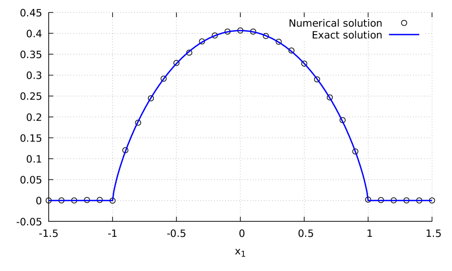
(a) Numerical solution of (5.5) with $k=0$.

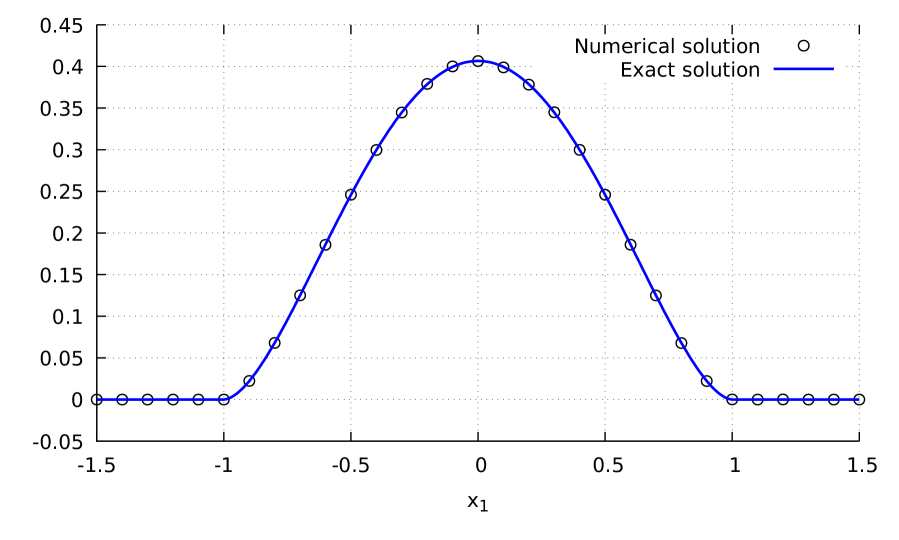
(b) Numerical solution of (5.5) with $k=1$.

Figure 1: Numerical solution of (5.5) in dimension $d=10$.

Nonlinear fractional PDE with gradient term

We consider the nonlinear PDE

$$\begin{cases}\displaystyle-\frac{\partial u}{\partial t}(t,x)=\Delta_{\alpha}u(t,x)+u(t,x)+e^{-t}\Psi_{k,\alpha}(x)\\ \hskip 65.44142pt\displaystyle+(2k+\alpha)e^{-2t}(1-\|x\|^{2})^{2k+\alpha-1}_{+}\sum_{j=1}^{d}x_{j}+u(t,x)\sum_{j=1}^{d}\frac{\partial u}{\partial x_{j}}(t,x)\vskip 6.0pt plus 2.0pt minus 2.0pt\\ u(T,x)=e^{-T}(1-\|x\|^{2})^{k+\alpha/2}_{+},\end{cases}{}$$ (5.6)

with $m=d$,

$$f(t,x,y,z_{1},\ldots,z_{d})=c_{0,\ldots,0}(t,x)+y(z_{1}+\cdots+z_{d}),$$

${\cal L}_{d}=\{(0,\ldots,0),(1,1,\ldots,0),\ldots,(1,0,\ldots,1)\}$,

$$c_{0,\ldots,0}(t,x)=e^{-t}\Psi_{k,\alpha}(x)+(2k+\alpha)e^{-2t}(1-\|x\|^{2})^{2k+\alpha-1}_{+}(x_{1}+\cdots+x_{d}),$$

and $c_{1,1,\ldots,0}(t,x)=\cdots=c_{1,0,\ldots,1}(t,x)=1$, whose explicit solution $u(t,x)$ is also given by (5.4) according to (5.3). In dimension $d=1$ the possible marks are $0$ and $1$, and the corresponding random trees branches into 0 branch, 1 branch, or 2 branches), as in the following random sample:

In dimension $d>1$ the tree expands into $d+2$ different types of branches, namely $0$ branch, one branch with mark $0$, and $d$ types of two branches with one branch bearing the mark $0$ and the other branch bearing a mark $i\in\{1,\dots,d\}$, which corresponds to the partial derivative with respect to $x_{i}$. In Figure 2 we plot the numerical solutions $u(t,x_{1},0,\ldots,0)$ of (5.6) obtained from (3.4) in terms of the first coordinate $x_{1}$ in dimension $d=2$, with $T=1$, $t=0.9$ and $\alpha=1.5$.

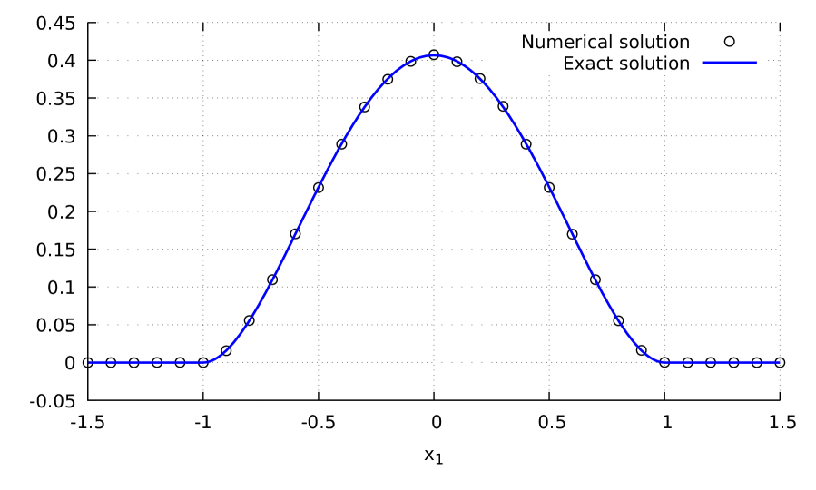
(a) Numerical solution of (5.6) with $k=1$.

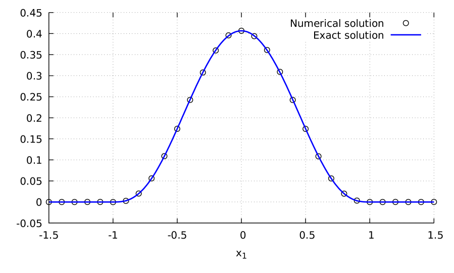
(b) Numerical solution of (5.6) with $k=2$.

Figure 2: Numerical solution of (5.6) in dimension $d=2$.

Fractional Burgers equation

We consider the fractional Burgers equation

$$\frac{\partial u}{\partial t}(t,x)+\kappa\Delta_{\alpha}u(t,x)-u(t,x)\sum_{j=1}^{d}\frac{\partial u}{\partial x_{j}}(t,x)=0,\qquad x=(x_{1},\ldots,x_{d})\in{}^{d},$$ (5.7)

with $m=d$, $f(t,x,y,z_{1},\ldots,z_{d})=y(z_{1}+\cdots+z_{d})$ and ${\cal L}_{d}=\{(1,1,\ldots,0),\ldots,(1,0,\ldots,1)\}$, $c_{1,1,\ldots,0}(t,x)=\cdots=c_{1,0,\ldots,1}(t,x)=1$, and one of the following two terminal conditions.

1. Half-space terminal condition

   $$u(T,x)=\mathbbm{1}_{[0,\infty)^{d}}(x_{1}),\qquad x=(x_{1},\ldots,x_{d})\in{}^{d}.$$ (5.8)

2. Product cosine terminal condition

   $$u(T,x)=\cos(x_{1})\cdots\cos(x_{d})\mathbbm{1}_{[-\pi/2,\pi/2]^{d}}(x_{1},\ldots,x_{d}),\qquad x=(x_{1},\ldots,x_{d})\in{}^{d}.$$ (5.9)

The random tree associated to this equation is a binary tree with $d$ types of branching. At each branching time, two branches are generated, one bearing the mark $0$ to represent $u$ and the other one bearing a mark $i\in\{1,\dots,d\}$ to represent $\partial u/\partial x_{i}$, which yields the following sample tree in dimension $d=1$.

In Figure 3 we plot the numerical solutions $u(t,x_{1},0)$ of (5.7) obtained from (3.4) in terms of the first coordinate $x_{1}$ in dimension $d=2$, with $\kappa=10$, $T=1$ and $\alpha=1.5$.

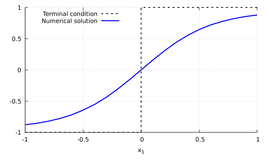
(a) Terminal condition (5.8) and $t=0.99$.

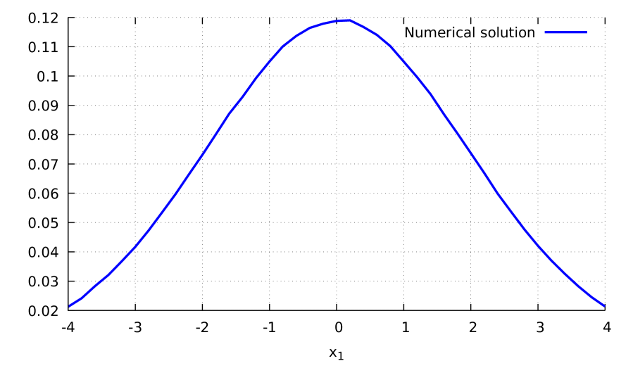
(b) Terminal condition (5.9) and $t=0.9$.

Figure 3: Numerical solution of (5.7) in dimension $d=2$.

Data availability statement

No new data were created during the study.