Revisiting Deep Learning Models for Tabular Data

Abstract

The existing literature on deep learning for tabular data proposes a wide range of novel architectures and reports competitive results on various datasets. However, the proposed models are usually not properly compared to each other and existing works often use different benchmarks and experiment protocols. As a result, it is unclear for both researchers and practitioners what models perform best. Additionally, the field still lacks effective baselines, that is, the easy-to-use models that provide competitive performance across different problems.

In this work, we perform an overview of the main families of DL architectures for tabular data and raise the bar of baselines in tabular DL by identifying two simple and powerful deep architectures. The first one is a ResNet-like architecture which turns out to be a strong baseline that is often missing in prior works. The second model is our simple adaptation of the Transformer architecture for tabular data, which outperforms other solutions on most tasks. Both models are compared to many existing architectures on a diverse set of tasks under the same training and tuning protocols. We also compare the best DL models with Gradient Boosted Decision Trees and conclude that there is still no universally superior solution. The source code is available at https://github.com/yandex-research/tabular-dl-revisiting-models.

1 Introduction

Due to the tremendous success of deep learning on such data domains as images, audio and texts (Goodfellow et al., 2016), there has been a lot of research interest to extend this success to problems with data stored in tabular format. In these problems, data points are represented as vectors of heterogeneous features, which is typical for industrial applications and ML competitions, where neural networks have a strong non-deep competitor in the form of GBDT (Chen and Guestrin, 2016; Prokhorenkova et al., 2018; Ke et al., 2017). Along with potentially higher performance, using deep learning for tabular data is appealing as it would allow constructing multi-modal pipelines for problems, where only one part of the input is tabular, and other parts include images, audio and other DL-friendly data. Such pipelines can then be trained end-to-end by gradient optimization for all modalities. For these reasons, a large number of DL solutions were recently proposed, and new models continue to emerge (Klambauer et al., 2017; Popov et al., 2020; Arik and Pfister, 2020; Song et al., 2019; Wang et al., 2017, 2020a; Badirli et al., 2020; Hazimeh et al., 2020; Huang et al., 2020a).

Unfortunately, due to the lack of established benchmarks (such as ImageNet (Deng et al., 2009) for computer vision or GLUE (Wang et al., 2019a) for NLP), existing papers use different datasets for evaluation and proposed DL models are often not adequately compared to each other. Therefore, from the current literature, it is unclear what DL model generally performs better than others and whether GBDT is surpassed by DL models. Additionally, despite the large number of novel architectures, the field still lacks simple and reliable solutions that allow achieving competitive performance with moderate effort and provide stable performance across many tasks. In that regard, Multilayer Perceptron (MLP) remains the main simple baseline for the field, however, it does not always represent a significant challenge for other competitors.

The described problems impede the research process and make the observations from the papers not conclusive enough. Therefore, we believe it is timely to review the recent developments from the field and raise the bar of baselines in tabular DL. We start with a hypothesis that well-studied DL architecture blocks may be underexplored in the context of tabular data and may be used to design better baselines. Thus, we take inspiration from well-known battle-tested architectures from other fields and obtain two simple models for tabular data. The first one is a ResNet-like architecture (He et al., 2015b) and the second one is FT-Transformer — our simple adaptation of the Transformer architecture (Vaswani et al., 2017) for tabular data. Then, we compare these models with many existing solutions on a diverse set of tasks under the same protocols of training and hyperparameters tuning. First, we reveal that none of the considered DL models can consistently outperform the ResNet-like model. Given its simplicity, it can serve as a strong baseline for future work. Second, FT-Transformer demonstrates the best performance on most tasks and becomes a new powerful solution for the field. Interestingly, FT-Transformer turns out to be a more universal architecture for tabular data: it performs well on a wider range of tasks than the more “conventional” ResNet and other DL models. Finally, we compare the best DL models to GBDT and conclude that there is still no universally superior solution.

We summarize the contributions of our paper as follows:

1. We thoroughly evaluate the main models for tabular DL on a diverse set of tasks to investigate their relative performance.

2. We demonstrate that a simple ResNet-like architecture is an effective baseline for tabular DL, which was overlooked by existing literature. Given its simplicity, we recommend this baseline for comparison in future tabular DL works.

3. We introduce FT-Transformer — a simple adaptation of the Transformer architecture for tabular data that becomes a new powerful solution for the field. We observe that it is a more universal architecture: it performs well on a wider range of tasks than other DL models.

4. We reveal that there is still no universally superior solution among GBDT and deep models.

2 Related work

The “shallow” state-of-the-art for problems with tabular data is currently ensembles of decision trees, such as GBDT (Gradient Boosting Decision Tree) (Friedman, 2001), which are typically the top-choice in various ML competitions. At the moment, there are several established GBDT libraries, such as XGBoost (Chen and Guestrin, 2016), LightGBM (Ke et al., 2017), CatBoost (Prokhorenkova et al., 2018), which are widely used by both ML researchers and practitioners. While these implementations vary in detail, on most of the tasks, their performances do not differ much (Prokhorenkova et al., 2018).

During several recent years, a large number of deep learning models for tabular data have been developed (Klambauer et al., 2017; Popov et al., 2020; Arik and Pfister, 2020; Song et al., 2019; Wang et al., 2017; Badirli et al., 2020; Hazimeh et al., 2020; Huang et al., 2020a). Most of these models can be roughly categorized into three groups, which we briefly describe below.

Differentiable trees. The first group of models is motivated by the strong performance of decision tree ensembles for tabular data. Since decision trees are not differentiable and do not allow gradient optimization, they cannot be used as a component for pipelines trained in the end-to-end fashion. To address this issue, several works (Kontschieder et al., 2015; Yang et al., 2018; Popov et al., 2020; Hazimeh et al., 2020) propose to “smooth” decision functions in the internal tree nodes to make the overall tree function and tree routing differentiable. While the methods of this family can outperform GBDT on some tasks (Popov et al., 2020), in our experiments, they do not consistently outperform ResNet.

Attention-based models. Due to the ubiquitous success of attention-based architectures for different domains (Vaswani et al., 2017; Dosovitskiy et al., 2021), several authors propose to employ attention-like modules for tabular DL as well (Arik and Pfister, 2020; Song et al., 2019; Huang et al., 2020a). In our experiments, we show that the properly tuned ResNet outperforms the existing attention-based models. Nevertheless, we identify an effective way to apply the Transformer architecture (Vaswani et al., 2017) to tabular data: the resulting architecture outperforms ResNet on most of the tasks.

Explicit modeling of multiplicative interactions. In the literature on recommender systems and click-through-rate prediction, several works criticize MLP since it is unsuitable for modeling multiplicative interactions between features (Beutel et al., 2018; Wang et al., 2017; Qin et al., 2021). Inspired by this motivation, some works (Beutel et al., 2018; Wang et al., 2017, 2020a) have proposed different ways to incorporate feature products into MLP. In our experiments, however, we do not find such methods to be superior to properly tuned baselines.

The literature also proposes some other architectural designs (Badirli et al., 2020; Klambauer et al., 2017) that cannot be explicitly assigned to any of the groups above. Overall, the community has developed a variety of models that are evaluated on different benchmarks and are rarely compared to each other. Our work aims to establish a fair comparison of them and identify the solutions that consistently provide high performance.

3 Models for tabular data problems

In this section, we describe the main deep architectures that we highlight in our work, as well as the existing solutions included in the comparison. Since we argue that the field needs strong easy-to-use baselines, we try to reuse well-established DL building blocks as much as possible when designing ResNet (section 3.2) and FT-Transformer (section 3.3). We hope this approach will result in conceptually familiar models that require less effort to achieve good performance. Additional discussion and technical details for all the models are provided in supplementary.

Notation. In this work, we consider supervised learning problems. $D{=}\{(x_{i},\ y_{i})\}_{i=1}^{n}$ denotes a dataset, where $x_{i}{=}(x_{i}^{(num)},\ x_{i}^{(cat)})\in\mathbb{X}$ represents numerical $x_{ij}^{(num)}$ and categorical $x_{ij}^{(cat)}$ features of an object and $y_{i}\in\mathbb{Y}$ denotes the corresponding object label. The total number of features is denoted as $k$. The dataset is split into three disjoint subsets: $D=D_{train}\ \cup\ D_{val}\ \cup\ D_{test}$, where $D_{train}$ is used for training, $D_{val}$ is used for early stopping and hyperparameter tuning, and $D_{test}$ is used for the final evaluation. We consider three types of tasks: binary classification $\mathbb{Y}=\{0,\ 1\}$, multiclass classification $\mathbb{Y}=\{1,\ \ldots,\ C\}$ and regression $\mathbb{Y}=\mathbb{R}$.

3.1 MLP

We formalize the “MLP” architecture in Equation 1.

$$\texttt{MLP}(x) =\texttt{Linear}\left(\texttt{MLPBlock}\left(\ldots\left(\texttt{MLPBlock}(x)\right)\right)\right)$$ (1)

$$\texttt{MLPBlock}(x) =\texttt{Dropout}(\texttt{ReLU}(\texttt{Linear}(x)))$$

3.2 ResNet

We are aware of one attempt to design a ResNet-like baseline (Klambauer et al., 2017) where the reported results were not competitive. However, given ResNet’s success story in computer vision (He et al., 2015b) and its recent achievements on NLP tasks (Sun and Iyyer, 2021), we give it a second try and construct a simple variation of ResNet as described in Equation 2. The main building block is simplified compared to the original architecture, and there is an almost clear path from the input to output which we find to be beneficial for the optimization. Overall, we expect this architecture to outperform MLP on tasks where deeper representations can be helpful.

$$\texttt{ResNet}(x) =\texttt{Prediction}\left(\texttt{ResNetBlock}\left(\ldots\left(\texttt{ResNetBlock}\left(\texttt{Linear}(x)\right)\right)\right)\right)$$ (2)

$$\texttt{ResNetBlock}(x) =x+\texttt{Dropout}(\texttt{Linear}(\texttt{Dropout}(\texttt{ReLU}(\texttt{Linear}(\texttt{BatchNorm}(x))))))$$

$$\texttt{Prediction}(x) =\texttt{Linear}\left(\texttt{ReLU}\left(\texttt{BatchNorm}\left(x\right)\right)\right)$$

3.3 FT-Transformer

In this section, we introduce FT-Transformer (Feature Tokenizer + Transformer) — a simple adaptation of the Transformer architecture (Vaswani et al., 2017) for the tabular domain. Figure 1 demonstrates the main parts of FT-Transformer. In a nutshell, our model transforms all features (categorical and numerical) to embeddings and applies a stack of Transformer layers to the embeddings. Thus, every Transformer layer operates on the feature level of one object. We compare FT-Transformer to conceptually similar AutoInt in section 5.2.

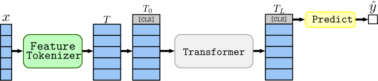
Figure 1: The FT-Transformer architecture. Firstly, Feature Tokenizer transforms features to embeddings. The embeddings are then processed by the Transformer module and the final representation of the [CLS] token is used for prediction.

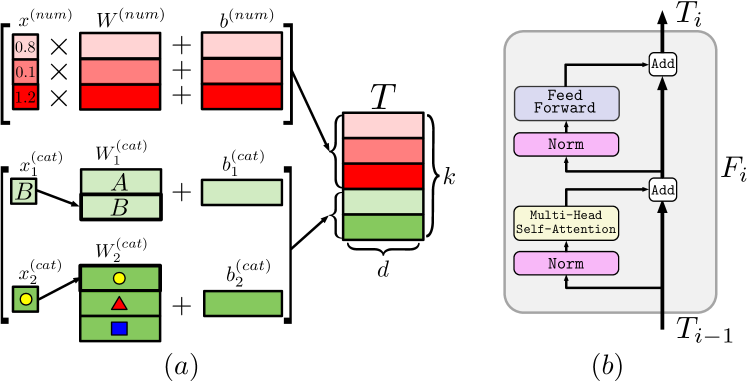
Figure 2: (a) Feature Tokenizer; in the example, there are three numerical and two categorical features; (b) One Transformer layer.

Feature Tokenizer. The Feature Tokenizer module (see Figure 2) transforms the input features $x$ to embeddings $T\in\mathbb{R}^{k\times d}$. The embedding for a given feature $x_{j}$ is computed as follows:

$$T_{j}=b_{j}+f_{j}(x_{j})\in\mathbb{R}^{d}\qquad f_{j}:\mathbb{X}_{j}\rightarrow\mathbb{R}^{d}.$$

where $b_{j}$ is the $j$-th feature bias, $f^{(num)}_{j}$ is implemented as the element-wise multiplication with the vector $W^{(num)}_{j}\in\mathbb{R}^{d}$ and $f^{(cat)}_{j}$ is implemented as the lookup table $W^{(cat)}_{j}\in\mathbb{R}^{S_{j}\times d}$ for categorical features. Overall:

$$T^{(num)}_{j}=b^{(num)}_{j}+x^{(num)}_{j}\cdot W^{(num)}_{j} \in\mathbb{R}^{d},$$

$$T^{(cat)}_{j}=b^{(cat)}_{j}+e_{j}^{T}W^{(cat)}_{j} \in\mathbb{R}^{d},$$

$$T=\mathtt{stack}\left[T^{(num)}_{1},\ \ldots,\ T^{(num)}_{k^{(num)}},\ T^{(cat)}_{1},\ \ldots,\ T^{(cat)}_{k^{(cat)}}\right] \in\mathbb{R}^{k\times d}.$$

where $e_{j}^{T}$ is a one-hot vector for the corresponding categorical feature.

Transformer. At this stage, the embedding of the [CLS] token (or “classification token”, or “output token”, see Devlin et al. (2019)) is appended to $T$ and $L$ Transformer layers $F_{1},\ \dotsc,\ F_{L}$ are applied:

$$T_{0}=\mathtt{stack}\left[{\texttt{[CLS]},\ T}\right]\qquad T_{i}=F_{i}(T_{i-1}).$$

We use the PreNorm variant for easier optimization (Wang et al., 2019b), see Figure 2. In the PreNorm setting, we also found it to be necessary to remove the first normalization from the first Transformer layer to achieve good performance. See the original paper (Vaswani et al., 2017) for the background on Multi-Head Self-Attention (MHSA) and the Feed Forward module. See supplementary for details such as activations, placement of normalizations and dropout modules (Srivastava et al., 2014).

Prediction. The final representation of the [CLS] token is used for prediction:

$$\hat{y}=\texttt{Linear}(\texttt{ReLU}(\texttt{LayerNorm}(T^{\texttt{[CLS]}}_{L}))).$$

Limitations. FT-Transformer requires more resources (both hardware and time) for training than simple models such as ResNet and may not be easily scaled to datasets when the number of features is “too large” (it is determined by the available hardware and time budget). Consequently, widespread usage of FT-Transformer for solving tabular data problems can lead to greater CO2 emissions produced by ML pipelines, since tabular data problems are ubiquitous. The main cause of the described problem lies in the quadratic complexity of the vanilla MHSA with respect to the number of features. However, the issue can be alleviated by using efficient approximations of MHSA (Tay et al., 2020). Additionally, it is still possible to distill FT-Transformer into simpler architectures for better inference performance. We report training times and the used hardware in supplementary.

3.4 Other models

In this section, we list the existing models designed specifically for tabular data that we include in the comparison.

• SNN (Klambauer et al., 2017). An MLP-like architecture with the SELU activation that enables training deeper models.

• NODE (Popov et al., 2020). A differentiable ensemble of oblivious decision trees.

• TabNet (Arik and Pfister, 2020). A recurrent architecture that alternates dynamical reweighing of features and conventional feed-forward modules.

• GrowNet (Badirli et al., 2020). Gradient boosted weak MLPs. The official implementation supports only classification and regression problems.

• DCN V2 (Wang et al., 2020a). Consists of an MLP-like module and the feature crossing module (a combination of linear layers and multiplications).

• AutoInt (Song et al., 2019). Transforms features to embeddings and applies a series of attention-based transformations to the embeddings.

• XGBoost (Chen and Guestrin, 2016). One of the most popular GBDT implementations.

• CatBoost (Prokhorenkova et al., 2018). GBDT implementation that uses oblivious decision trees (Lou and Obukhov, 2017) as weak learners.

4 Experiments

In this section, we compare DL models to each other as well as to GBDT. Note that in the main text, we report only the key results. In supplementary, we provide: (1) the results for all models on all datasets; (2) information on hardware; (3) training times for ResNet and FT-Transformer.

4.1 Scope of the comparison

In our work, we focus on the relative performance of different architectures and do not employ various model-agnostic DL practices, such as pretraining, additional loss functions, data augmentation, distillation, learning rate warmup, learning rate decay and many others. While these practices can potentially improve the performance, our goal is to evaluate the impact of inductive biases imposed by the different model architectures.

4.2 Datasets

We use a diverse set of eleven public datasets (see supplementary for the detailed description). For each dataset, there is exactly one train-validation-test split, so all algorithms use the same splits. The datasets include: California Housing (CA, real estate data, Kelley Pace and Barry (1997)), Adult (AD, income estimation, Kohavi (1996)), Helena (HE, anonymized dataset, Guyon et al. (2019)), Jannis (JA, anonymized dataset, Guyon et al. (2019)), Higgs (HI, simulated physical particles, Baldi et al. (2014); we use the version with 98K samples available at the OpenML repository (Vanschoren et al., 2014)), ALOI (AL, images, Geusebroek et al. (2005)), Epsilon (EP, simulated physics experiments), Year (YE, audio features, Bertin-Mahieux et al. (2011)), Covertype (CO, forest characteristics, Blackard and Dean. (2000)), Yahoo (YA, search queries, Chapelle and Chang (2011)), Microsoft (MI, search queries, Qin and Liu (2013)). We follow the pointwise approach to learning-to-rank and treat ranking problems (Microsoft, Yahoo) as regression problems. The dataset properties are summarized in Table 1.

Table 1: Dataset properties. Notation: “RMSE” ~ root-mean-square error, “Acc.” ~ accuracy.

	CA	AD	HE	JA	HI	AL	EP	YE	CO	YA	MI
#objects	20640	48842	65196	83733	98050	108000	500000	515345	581012	709877	1200192
#num. features	8	6	27	54	28	128	2000	90	54	699	136
#cat. features	0	8	0	0	0	0	0	0	0	0	0
metric	RMSE	Acc.	Acc.	Acc.	Acc.	Acc.	Acc.	RMSE	Acc.	RMSE	RMSE
#classes	–	2	100	4	2	1000	2	–	7	–	–

4.3 Implementation details

Data preprocessing. Data preprocessing is known to be vital for DL models. For each dataset, the same preprocessing was used for all deep models for a fair comparison. By default, we used the quantile transformation from the Scikit-learn library (Pedregosa et al., 2011). We apply standardization (mean subtraction and scaling) to Helena and ALOI. The latter one represents image data, and standardization is a common practice in computer vision. On the Epsilon dataset, we observed preprocessing to be detrimental to deep models’ performance, so we use the raw features on this dataset. We apply standardization to regression targets for all algorithms.

Tuning. For every dataset, we carefully tune each model’s hyperparameters. The best hyperparameters are the ones that perform best on the validation set, so the test set is never used for tuning. For most algorithms, we use the Optuna library (Akiba et al., 2019) to run Bayesian optimization (the Tree-Structured Parzen Estimator algorithm), which is reported to be superior to random search (Turner et al., 2021). For the rest, we iterate over predefined sets of configurations recommended by corresponding papers. We provide parameter spaces and grids in supplementary. We set the budget for Optuna-based tuning in terms of iterations and provide additional analysis on setting the budget in terms of time in supplementary.

Evaluation. For each tuned configuration, we run 15 experiments with different random seeds and report the performance on the test set. For some algorithms, we also report the performance of default configurations without hyperparameter tuning.

Ensembles. For each model, on each dataset, we obtain three ensembles by splitting the 15 single models into three disjoint groups of equal size and averaging predictions of single models within each group.

Neural networks. We minimize cross-entropy for classification problems and mean squared error for regression problems. For TabNet and GrowNet, we follow the original implementations and use the Adam optimizer (Kingma and Ba, 2017). For all other algorithms, we use the AdamW optimizer (Loshchilov and Hutter, 2019). We do not apply learning rate schedules. For each dataset, we use a predefined batch size for all algorithms unless special instructions on batch sizes are given in the corresponding papers (see supplementary). We continue training until there are $\texttt{patience}+1$ consecutive epochs without improvements on the validation set; we set $\texttt{patience}=16$ for all algorithms.

Categorical features. For XGBoost, we use one-hot encoding. For CatBoost, we employ the built-in support for categorical features. For Neural Networks, we use embeddings of the same dimensionality for all categorical features.

4.4 Comparing DL models

Table 2: Results for DL models. The metric values averaged over 15 random seeds are reported. See supplementary for standard deviations. For each dataset, top results are in bold. “Top” means “the gap between this result and the result with the best score is not statistically significant”. For each dataset, ranks are calculated by sorting the reported scores; the “rank” column reports the average rank across all datasets. Notation: FT-T ~ FT-Transformer, ↓ ~ RMSE, ↑ ~ accuracy

	CA ↓	AD ↑	HE ↑	JA ↑	HI ↑	AL ↑	EP ↑	YE ↓	CO ↑	YA ↓	MI ↓	rank (std)
TabNet	$0.510$	$0.850$	$0.378$	$0.723$	$0.719$	$0.954$	$0.8896$	$8.909$	$0.957$	$0.823$	$0.751$	$7.5$ $(2.0)$
SNN	$0.493$	$0.854$	$0.373$	$0.719$	$0.722$	$0.954$	$0.8975$	$8.895$	$0.961$	$0.761$	$0.751$	$6.4$ $(1.4)$
AutoInt	$0.474$	$\mathbf{0.859}$	$0.372$	$0.721$	$0.725$	$0.945$	$0.8949$	$8.882$	$0.934$	$0.768$	$0.750$	$5.7$ $(2.3)$
GrowNet	$0.487$	$\mathbf{0.857}$	–	–	$0.722$	–	$0.8970$	$8.827$	–	$0.765$	$0.751$	$5.7$ $(2.2)$
MLP	$0.499$	$0.852$	$0.383$	$0.719$	$0.723$	$0.954$	$0.8977$	$8.853$	$0.962$	$0.757$	$0.747$	$4.8$ $(1.9)$
DCN2	$0.484$	$0.853$	$0.385$	$0.716$	$0.723$	$0.955$	$0.8977$	$8.890$	$0.965$	$0.757$	$0.749$	$4.7$ $(2.0)$
NODE	$0.464$	$\mathbf{0.858}$	$0.359$	$0.727$	$0.726$	$0.918$	$0.8958$	$\mathbf{8.784}$	$0.958$	$\mathbf{0.753}$	$\mathbf{0.745}$	$3.9$ $(2.8)$
ResNet	$0.486$	$0.854$	$\mathbf{0.396}$	$0.728$	$0.727$	$\mathbf{0.963}$	$0.8969$	$8.846$	$0.964$	$0.757$	$0.748$	$3.3$ $(1.8)$
FT-T	$\mathbf{0.459}$	$\mathbf{0.859}$	$0.391$	$\mathbf{0.732}$	$\mathbf{0.729}$	$0.960$	$\mathbf{0.8982}$	$8.855$	$\mathbf{0.970}$	$0.756$	$0.746$	$1.8$ $(1.2)$

Table 2 reports the results for deep architectures.
The main takeaways:

• MLP is still a good sanity check

• ResNet turns out to be an effective baseline that none of the competitors can consistently outperform.

• FT-Transformer performs best on most tasks and becomes a new powerful solution for the field.

• Tuning makes simple models such as MLP and ResNet competitive, so we recommend tuning baselines when possible. Luckily, today, it is more approachable with libraries such as Optuna (Akiba et al., 2019).

Among other models, NODE (Popov et al., 2020) is the only one that demonstrates high performance on several tasks. However, it is still inferior to ResNet on six datasets (Helena, Jannis, Higgs, ALOI, Epsilon, Covertype), while being a more complex solution. Moreover, it is not a truly “single” model; in fact, it often contains significantly more parameters than ResNet and FT-Transformer and has an ensemble-like structure. We illustrate that by comparing ensembles in Table 3. The results indicate that FT-Transformer and ResNet benefit more from ensembling; in this regime, FT-Transformer outperforms NODE and the gap between ResNet and NODE is significantly reduced. Nevertheless, NODE remains a prominent solution among tree-based approaches.

Table 3: Results for ensembles of DL models with the highest ranks (see Table 2). For each model-dataset pair, the metric value averaged over three ensembles is reported. See supplementary for standard deviations. Depending on the dataset, the highest accuracy or the lowest RMSE is in bold. Due to the limited precision, some different values are represented with the same figures. Notation: ↓ ~ RMSE, ↑ ~ accuracy.

	CA ↓	AD ↑	HE ↑	JA ↑	HI ↑	AL ↑	EP ↑	YE ↓	CO ↑	YA ↓	MI ↓
NODE	$0.461$	$0.860$	$0.361$	$0.730$	$0.727$	$0.921$	$0.8970$	$\mathbf{8.716}$	$0.965$	$0.750$	$0.744$
ResNet	$0.478$	$0.857$	$0.398$	$0.734$	$0.731$	$0.966$	$0.8976$	$8.770$	$0.967$	$0.751$	$0.745$
FT-Transformer	$\mathbf{0.448}$	$\mathbf{0.860}$	$\mathbf{0.398}$	$\mathbf{0.739}$	$\mathbf{0.731}$	$\mathbf{0.967}$	$\mathbf{0.8984}$	$8.751$	$\mathbf{0.973}$	$\mathbf{0.747}$	$\mathbf{0.743}$

4.5 Comparing DL models and GBDT

In this section, our goal is to check whether DL models are conceptually ready to outperform GBDT. To this end, we compare the best possible metric values that one can achieve using GBDT or DL models, without taking speed and hardware requirements into account (undoubtedly, GBDT is a more lightweight solution). We accomplish that by comparing ensembles instead of single models since GBDT is essentially an ensembling technique and we expect that deep architectures will benefit more from ensembling (Fort et al., 2020). We report the results in Table 4.

Table 4: Results for ensembles of GBDT and the main DL models. For each model-dataset pair, the metric value averaged over three ensembles is reported. See supplementary for standard deviations. Notation follows Table 3.

	CA ↓	AD ↑	HE ↑	JA ↑	HI ↑	AL ↑	EP ↑	YE ↓	CO ↑	YA ↓	MI ↓
Default hyperparameters
XGBoost	$0.462$	$\mathbf{0.874}$	$0.348$	$0.711$	$0.717$	$0.924$	$0.8799$	$9.192$	$0.964$	$0.761$	$0.751$
CatBoost	$\mathbf{0.428}$	$0.873$	$0.386$	$0.724$	$0.728$	$0.948$	$0.8893$	$8.885$	$0.910$	$0.749$	$0.744$
FT-Transformer	$0.454$	$0.860$	$\mathbf{0.395}$	$\mathbf{0.734}$	$\mathbf{0.731}$	$\mathbf{0.966}$	$\mathbf{0.8969}$	$\mathbf{8.727}$	$\mathbf{0.973}$	$\mathbf{0.747}$	$\mathbf{0.742}$
Tuned hyperparameters
XGBoost	$0.431$	$0.872$	$0.377$	$0.724$	$0.728$	–	$0.8861$	$8.819$	$0.969$	$\mathbf{0.732}$	$0.742$
CatBoost	$\mathbf{0.423}$	$\mathbf{0.874}$	$0.388$	$0.727$	$0.729$	–	$0.8898$	$8.837$	$0.968$	$0.740$	$\mathbf{0.741}$
ResNet	$0.478$	$0.857$	$0.398$	$0.734$	$0.731$	$0.966$	$0.8976$	$8.770$	$0.967$	$0.751$	$0.745$
FT-Transformer	$0.448$	$0.860$	$\mathbf{0.398}$	$\mathbf{0.739}$	$\mathbf{0.731}$	$\mathbf{0.967}$	$\mathbf{0.8984}$	$\mathbf{8.751}$	$\mathbf{0.973}$	$0.747$	$0.743$

Default hyperparameters. We start with the default configurations to check the “out-of-the-box” performance, which is an important practical scenario. The default FT-Transformer implies a configuration with all hyperparameters set to some specific values that we provide in supplementary. Table 4 demonstrates that the ensemble of FT-Transformers mostly outperforms the ensembles of GBDT, which is not the case for only two datasets (California Housing, Adult). Interestingly, the ensemble of default FT-Transformers performs quite on par with the ensembles of tuned FT-Transformers.
The main takeaway: FT-Transformer allows building powerful ensembles out of the box.

Tuned hyperparameters. Once hyperparameters are properly tuned, GBDTs start dominating on some datasets (California Housing, Adult, Yahoo; see Table 4). In those cases, the gaps are significant enough to conclude that DL models do not universally outperform GBDT. Importantly, the fact that DL models outperform GBDT on most of the tasks does not mean that DL solutions are “better” in any sense. In fact, it only means that the constructed benchmark is slightly biased towards “DL-friendly” problems. Admittedly, GBDT remains an unsuitable solution to multiclass problems with a large number of classes. Depending on the number of classes, GBDT can demonstrate unsatisfactory performance (Helena) or even be untunable due to extremely slow training (ALOI).
The main takeaways:

• there is still no universal solution among DL models and GBDT

• DL research efforts aimed at surpassing GBDT should focus on datasets where GBDT outperforms state-of-the-art DL solutions. Note that including “DL-friendly” problems is still important to avoid degradation on such problems.

4.6 An intriguing property of FT-Transformer

Table 4 tells one more important story. Namely, FT-Transformer delivers most of its advantage over the “conventional” DL model in the form of ResNet exactly on those problems where GBDT is superior to ResNet (California Housing, Adult, Covertype, Yahoo, Microsoft) while performing on par with ResNet on the remaining problems. In other words, FT-Transformer provides competitive performance on all tasks, while GBDT and ResNet perform well only on some subsets of the tasks. This observation may be the evidence that FT-Transformer is a more “universal” model for tabular data problems. We develop this intuition further in section 5.1. Note that the described phenomenon is not related to ensembling and is observed for single models too (see supplementary).

5 Analysis

5.1 When FT-Transformer is better than ResNet?

In this section, we make the first step towards understanding the difference in behavior between FT-Transformer and ResNet, which was first observed in section 4.6. To achieve that, we design a sequence of synthetic tasks where the difference in performance of the two models gradually changes from negligible to dramatic. Namely, we generate and fix objects $\{x_{i}\}_{i=1}^{n}$, perform the train-val-test split once and interpolate between two regression targets: $f_{GBDT}$, which is supposed to be easier for GBDT and $f_{DL}$, which is expected to be easier for ResNet. Formally, for one object:

$$x\sim\mathcal{N}(0,I_{k}),\qquad y=\alpha\cdot f_{GBDT}(x)+(1-\alpha)\cdot f_{DL}(x).$$

Figure 3: Test RMSE averaged over five seeds (shadows represent std. dev.). One $\alpha$ corresponds to one task; each task has the same set of train, validation and test features, but different targets.

where $f_{GBDT}(x)$ is an average prediction of 30 randomly constructed decision trees, and $f_{DL}(x)$ is an MLP with three randomly initialized hidden layers. Both $f_{GBDT}$ and $f_{DL}$ are generated once, i.e. the same functions are applied to all objects (see supplementary for details). The resulting targets are standardized before training. The results are visualized in Figure 3. ResNet and FT-Transformer perform similarly well on the ResNet-friendly tasks and outperform CatBoost on those tasks. However, the ResNet’s relative performance drops significantly when the target becomes more GBDT friendly. By contrast, FT-Transformer yields competitive performance across the whole range of tasks.

The conducted experiment reveals a type of functions that are better approximated by FT-Transformer than by ResNet. Additionally, the fact that these functions are based on decision trees correlates with the observations in section 4.6 and the results in Table 4, where FT-Transformer shows the most convincing improvements over ResNet exactly on those datasets where GBDT outperforms ResNet.

5.2 Ablation study

In this section, we test some design choices of FT-Transformer.

First, we compare FT-Transformer with AutoInt (Song et al., 2019), since it is the closest competitor in its spirit. AutoInt also converts all features to embeddings and applies self-attention on top of them. However, in its details, AutoInt significantly differs from FT-Transformer: its embedding layer does not include feature biases, its backbone significantly differs from the vanilla Transformer (Vaswani et al., 2017), and the inference mechanism does not use the [CLS] token.

Second, we check whether feature biases in Feature Tokenizer are essential for good performance.

We tune and evaluate FT-Transformer without feature biases following the same protocol as in section 4.3 and reuse the remaining numbers from Table 2. The results averaged over 15 runs are reported in Table 5 and demonstrate both the superiority of the Transformer’s backbone to that of AutoInt and the necessity of feature biases.

Table 5: The results of the comparison between FT-Transformer and two attention-based alternatives: AutoInt and FT-Transformer without feature biases. Notation follows Table 2.

	CA ↓	HE ↑	JA ↑	HI ↑	AL ↑	YE ↓	CO ↑	MI ↓
AutoInt	$0.474$	$0.372$	$0.721$	$0.725$	$0.945$	$8.882$	$0.934$	$0.750$
FT-Transformer (w/o feature biases)	$0.470$	$0.381$	$0.724$	$\mathbf{0.727}$	$0.958$	$\mathbf{8.843}$	$0.964$	$0.751$
FT-Transformer	$\mathbf{0.459}$	$\mathbf{0.391}$	$\mathbf{0.732}$	$\mathbf{0.729}$	$\mathbf{0.960}$	$\mathbf{8.855}$	$\mathbf{0.970}$	$\mathbf{0.746}$

5.3 Obtaining feature importances from attention maps

In this section, we evaluate attention maps as a source of information on feature importances for FT-Transformer for a given set of samples. For the $i$-th sample, we calculate the average attention map $p_{i}$ for the [CLS] token from Transformer’s forward pass. Then, the obtained individual distributions are averaged into one distribution $p$ that represents the feature importances:

$$p=\frac{1}{n_{samples}}\sum_{i}p_{i}\qquad p_{i}=\frac{1}{n_{heads}\times L}\sum_{h,l}p_{ihl}.$$

where $p_{ihl}$ is the $h$-th head’s attention map for the [CLS] token from the forward pass of the $l$-th layer on the $i$-th sample. The main advantage of the described heuristic technique is its efficiency: it requires a single forward for one sample.

In order to evaluate our approach, we compare it with Integrated Gradients (IG, Sundararajan et al. (2017)), a general technique applicable to any differentiable model. We use permutation test (PT, Breiman (2001)) as a reasonable interpretable method that allows us to establish a constructive metric, namely, rank correlation. We run all the methods on the train set and summarize results in Table 6. Interestingly, the proposed method yields reasonable feature importances and performs similarly to IG (note that this does not imply similarity to IG’s feature importances). Given that IG can be orders of magnitude slower and the “baseline” in the form of PT requires $(n_{features}+1)$ forward passes (versus one for the proposed method), we conclude that the simple averaging of attention maps can be a good choice in terms of cost-effectiveness.

Table 6: Rank correlation (takes values in $[-1,\ 1]$) between permutation test’s feature importances ranking and two alternative rankings: Attention Maps (AM) and Integrated Gradients (IG). Means and standard deviations over five runs are reported.

	CA	HE	JA	HI	AL	YE	CO	MI
AM	$0.81\ (0.05)$	$0.77\ (0.03)$	$0.78\ (0.05)$	$0.91\ (0.03)$	$0.84\ (0.01)$	$0.92\ (0.01)$	$0.84\ (0.04)$	$0.86\ (0.02)$
IG	$0.84\ (0.08)$	$0.74\ (0.03)$	$0.75\ (0.04)$	$0.72\ (0.03)$	$0.89\ (0.01)$	$0.50\ (0.03)$	$0.90\ (0.02)$	$0.56\ (0.02)$

6 Conclusion

In this work, we have investigated the status quo in the field of deep learning for tabular data and improved the state of baselines in tabular DL. First, we have demonstrated that a simple ResNet-like architecture can serve as an effective baseline. Second, we have proposed FT-Transformer — a simple adaptation of the Transformer architecture that outperforms other DL solutions on most of the tasks. We have also compared the new baselines with GBDT and demonstrated that GBDT still dominates on some tasks. The code and all the details of the study are open-sourced , and we hope that our evaluation and two simple models (ResNet and FT-Transformer) will serve as a basis for further developments on tabular DL.

Supplementary material

A Software and hardware

For most model-dataset pairs the workflow was as follows:

• tune the model on any suitable hardware

• evaluate the tuned model on one or more NVidia Tesla V100 32Gb

All the experiments were conducted under the same conditions in terms of software versions. For almost all experiments the used hardware can be found in the source code.

B Data

B.1 Datasets

Table 7: Datasets description

Name	Abbr	# Train	# Validation	# Test	# Num	# Cat	Task type	Batch size
California Housing	CA	$13209$	$3303$	$4128$	$8$	$0$	Regression	256
Adult	AD	$26048$	$6513$	$16281$	$6$	$8$	Binclass	256
Helena	HE	$41724$	$10432$	$13040$	$27$	$0$	Multiclass	512
Jannis	JA	$53588$	$13398$	$16747$	$54$	$0$	Multiclass	512
Higgs Small	HI	$62752$	$15688$	$19610$	$28$	$0$	Binclass	512
ALOI	AL	$69120$	$17280$	$21600$	$128$	$0$	Multiclass	512
Epsilon	EP	$320000$	$80000$	$100000$	$2000$	$0$	Binclass	1024
Year	YE	$370972$	$92743$	$51630$	$90$	$0$	Regression	1024
Covtype	CO	$371847$	$92962$	$116203$	$54$	$0$	Multiclass	1024
Yahoo	YA	$473134$	$71083$	$165660$	$699$	$0$	Regression	1024
Microsoft	MI	$723412$	$235259$	$241521$	$136$	$0$	Regression	1024

B.2 Preprocessing

For regression problems, we standardize the target values:

$$y_{new}=\frac{y_{old}-\mathtt{mean}(y_{train}))}{\mathtt{std}(y_{train})}$$ (3)

The feature preprocessing for DL models is described in the main text. Note that we add noise from $\mathcal{N}(0,1e-3)$ to train numerical features for calculating the parameters (quantiles) of the quantile preprocessing as a workaround for features with few distinct values (see the source code for the exact implementation). The preprocessing is then applied to original features. We do not preprocess features for GBDTs, since this family of algorithms is insensitive to feature shifts and scaling.

C Results for all algorithms on all datasets

To measure statistical significance in the main text and in the tables in this section, we use the one-sided Wilcoxon (1945) test with $p=0.01$.

Table 9 and Table 9 report all results for all models on all datasets.

Table 8: Results for single models with standard deviations. For each dataset, top results for baseline neural networks are in bold, top results for baseline neural networks and FT-Transformer are in blue, the overall top results are in red. “Top” means “the gap between this result and the result with the best mean score is not statistically significant”. “d” stands for “default”. The remaining notation follows those from the main text. Best viewed in colors.

	CA ↓	AD ↑	HE ↑	JA ↑	HI ↑	AL ↑	EP ↑	YE ↓	CO ↑	YA ↓	MI ↓
Baseline Neural Networks
TabNet	$0.510\scriptscriptstyle\pm\scriptstyle 7.6e\text{-}3$	$0.850\scriptscriptstyle\pm\scriptstyle 5.2e\text{-}3$	$0.378\scriptscriptstyle\pm\scriptstyle 1.7e\text{-}3$	$0.723\scriptscriptstyle\pm\scriptstyle 3.5e\text{-}3$	$0.719\scriptscriptstyle\pm\scriptstyle 1.7e\text{-}3$	$0.954\scriptscriptstyle\pm\scriptstyle 1.0e\text{-}3$	$0.8896\scriptscriptstyle\pm\scriptstyle 3.1e\text{-}3$	$8.909\scriptscriptstyle\pm\scriptstyle 2.3e\text{-}2$	$0.957\scriptscriptstyle\pm\scriptstyle 7.5e\text{-}3$	$0.823\scriptscriptstyle\pm\scriptstyle 9.2e\text{-}3$	$0.751\scriptscriptstyle\pm\scriptstyle 9.4e\text{-}4$
SNN	$0.493\scriptscriptstyle\pm\scriptstyle 4.6e\text{-}3$	$0.854\scriptscriptstyle\pm\scriptstyle 1.8e\text{-}3$	$0.373\scriptscriptstyle\pm\scriptstyle 2.8e\text{-}3$	$0.719\scriptscriptstyle\pm\scriptstyle 1.6e\text{-}3$	$0.722\scriptscriptstyle\pm\scriptstyle 2.2e\text{-}3$	$0.954\scriptscriptstyle\pm\scriptstyle 1.6e\text{-}3$	$\mathbf{0.8975\scriptscriptstyle\pm\scriptstyle 2.4e\text{-}4}$	$8.895\scriptscriptstyle\pm\scriptstyle 1.9e\text{-}2$	$0.961\scriptscriptstyle\pm\scriptstyle 2.0e\text{-}3$	$0.761\scriptscriptstyle\pm\scriptstyle 5.3e\text{-}4$	$0.751\scriptscriptstyle\pm\scriptstyle 5.2e\text{-}4$
AutoInt	$0.474\scriptscriptstyle\pm\scriptstyle 3.3e\text{-}3$	$\mathbf{{\color[rgb]{0,0,1}0.859\scriptscriptstyle\pm\scriptstyle 1.5e\text{-}3}}$	$0.372\scriptscriptstyle\pm\scriptstyle 2.5e\text{-}3$	$0.721\scriptscriptstyle\pm\scriptstyle 2.3e\text{-}3$	$\mathbf{0.725\scriptscriptstyle\pm\scriptstyle 1.7e\text{-}3}$	$0.945\scriptscriptstyle\pm\scriptstyle 1.3e\text{-}3$	$0.8949\scriptscriptstyle\pm\scriptstyle 5.8e\text{-}4$	$8.882\scriptscriptstyle\pm\scriptstyle 3.3e\text{-}2$	$0.934\scriptscriptstyle\pm\scriptstyle 3.5e\text{-}3$	$0.768\scriptscriptstyle\pm\scriptstyle 1.1e\text{-}3$	$0.750\scriptscriptstyle\pm\scriptstyle 6.1e\text{-}4$
GrowNet	$0.487\scriptscriptstyle\pm\scriptstyle 7.1e\text{-}3$	$\mathbf{{\color[rgb]{0,0,1}0.857\scriptscriptstyle\pm\scriptstyle 1.9e\text{-}3}}$	–	–	$0.722\scriptscriptstyle\pm\scriptstyle 1.6e\text{-}3$	–	$0.8970\scriptscriptstyle\pm\scriptstyle 5.7e\text{-}4$	$8.827\scriptscriptstyle\pm\scriptstyle 3.8e\text{-}2$	–	$0.765\scriptscriptstyle\pm\scriptstyle 1.2e\text{-}3$	$0.751\scriptscriptstyle\pm\scriptstyle 4.7e\text{-}4$
MLP	$0.499\scriptscriptstyle\pm\scriptstyle 2.9e\text{-}3$	$0.852\scriptscriptstyle\pm\scriptstyle 1.9e\text{-}3$	$0.383\scriptscriptstyle\pm\scriptstyle 2.6e\text{-}3$	$0.719\scriptscriptstyle\pm\scriptstyle 1.3e\text{-}3$	$0.723\scriptscriptstyle\pm\scriptstyle 1.8e\text{-}3$	$0.954\scriptscriptstyle\pm\scriptstyle 1.4e\text{-}3$	$\mathbf{0.8977\scriptscriptstyle\pm\scriptstyle 4.1e\text{-}4}$	$8.853\scriptscriptstyle\pm\scriptstyle 3.1e\text{-}2$	$0.962\scriptscriptstyle\pm\scriptstyle 1.1e\text{-}3$	$0.757\scriptscriptstyle\pm\scriptstyle 3.5e\text{-}4$	$0.747\scriptscriptstyle\pm\scriptstyle 3.3e\text{-}4$
DCN2	$0.484\scriptscriptstyle\pm\scriptstyle 2.4e\text{-}3$	$0.853\scriptscriptstyle\pm\scriptstyle 3.9e\text{-}3$	$0.385\scriptscriptstyle\pm\scriptstyle 3.0e\text{-}3$	$0.716\scriptscriptstyle\pm\scriptstyle 1.5e\text{-}3$	$0.723\scriptscriptstyle\pm\scriptstyle 1.3e\text{-}3$	$0.955\scriptscriptstyle\pm\scriptstyle 1.2e\text{-}3$	$\mathbf{0.8977\scriptscriptstyle\pm\scriptstyle 2.6e\text{-}4}$	$8.890\scriptscriptstyle\pm\scriptstyle 2.8e\text{-}2$	$\mathbf{0.965\scriptscriptstyle\pm\scriptstyle 1.0e\text{-}3}$	$0.757\scriptscriptstyle\pm\scriptstyle 1.9e\text{-}3$	$0.749\scriptscriptstyle\pm\scriptstyle 5.8e\text{-}4$
NODE	$\mathbf{0.464\scriptscriptstyle\pm\scriptstyle 1.5e\text{-}3}$	$\mathbf{{\color[rgb]{0,0,1}0.858\scriptscriptstyle\pm\scriptstyle 1.6e\text{-}3}}$	$0.359\scriptscriptstyle\pm\scriptstyle 2.0e\text{-}3$	$\mathbf{0.727\scriptscriptstyle\pm\scriptstyle 1.6e\text{-}3}$	$\mathbf{0.726\scriptscriptstyle\pm\scriptstyle 1.3e\text{-}3}$	$0.918\scriptscriptstyle\pm\scriptstyle 5.4e\text{-}3$	$0.8958\scriptscriptstyle\pm\scriptstyle 4.7e\text{-}4$	$\mathbf{{\color[rgb]{1,0,0}8.784\scriptscriptstyle\pm\scriptstyle 1.6e\text{-}2}}$	$0.958\scriptscriptstyle\pm\scriptstyle 1.1e\text{-}3$	$\mathbf{{\color[rgb]{0,0,1}0.753\scriptscriptstyle\pm\scriptstyle 2.5e\text{-}4}}$	$\mathbf{{\color[rgb]{0,0,1}0.745\scriptscriptstyle\pm\scriptstyle 2.0e\text{-}4}}$
ResNet	$0.486\scriptscriptstyle\pm\scriptstyle 2.9e\text{-}3$	$0.854\scriptscriptstyle\pm\scriptstyle 1.7e\text{-}3$	$\mathbf{{\color[rgb]{1,0,0}0.396\scriptscriptstyle\pm\scriptstyle 1.7e\text{-}3}}$	$\mathbf{0.728\scriptscriptstyle\pm\scriptstyle 1.5e\text{-}3}$	$\mathbf{0.727\scriptscriptstyle\pm\scriptstyle 1.7e\text{-}3}$	$\mathbf{{\color[rgb]{1,0,0}0.963\scriptscriptstyle\pm\scriptstyle 7.5e\text{-}4}}$	$0.8969\scriptscriptstyle\pm\scriptstyle 4.4e\text{-}4$	$8.846\scriptscriptstyle\pm\scriptstyle 2.4e\text{-}2$	$\mathbf{0.964\scriptscriptstyle\pm\scriptstyle 1.1e\text{-}3}$	$0.757\scriptscriptstyle\pm\scriptstyle 6.2e\text{-}4$	$0.748\scriptscriptstyle\pm\scriptstyle 3.1e\text{-}4$
FT-Transformer
FT-Transformerd	$0.469\scriptscriptstyle\pm\scriptstyle 3.8e\text{-}3$	$0.857\scriptscriptstyle\pm\scriptstyle 1.1e\text{-}3$	$0.381\scriptscriptstyle\pm\scriptstyle 2.4e\text{-}3$	$0.725\scriptscriptstyle\pm\scriptstyle 2.3e\text{-}3$	$0.725\scriptscriptstyle\pm\scriptstyle 1.8e\text{-}3$	$0.953\scriptscriptstyle\pm\scriptstyle 1.1e\text{-}3$	$0.8959\scriptscriptstyle\pm\scriptstyle 4.9e\text{-}4$	$8.889\scriptscriptstyle\pm\scriptstyle 4.6e\text{-}2$	$0.967\scriptscriptstyle\pm\scriptstyle 7.9e\text{-}4$	$0.756\scriptscriptstyle\pm\scriptstyle 8.2e\text{-}4$	$0.747\scriptscriptstyle\pm\scriptstyle 7.9e\text{-}4$
FT-Transformer	$\mathbf{{\color[rgb]{0,0,1}0.459\scriptscriptstyle\pm\scriptstyle 3.5e\text{-}3}}$	$\mathbf{{\color[rgb]{0,0,1}0.859\scriptscriptstyle\pm\scriptstyle 1.0e\text{-}3}}$	$0.391\scriptscriptstyle\pm\scriptstyle 1.2e\text{-}3$	$\mathbf{{\color[rgb]{1,0,0}0.732\scriptscriptstyle\pm\scriptstyle 2.0e\text{-}3}}$	$\mathbf{{\color[rgb]{1,0,0}0.729\scriptscriptstyle\pm\scriptstyle 1.5e\text{-}3}}$	$0.960\scriptscriptstyle\pm\scriptstyle 1.1e\text{-}3$	$\mathbf{{\color[rgb]{1,0,0}0.8982\scriptscriptstyle\pm\scriptstyle 2.8e\text{-}4}}$	$8.855\scriptscriptstyle\pm\scriptstyle 3.1e\text{-}2$	$\mathbf{{\color[rgb]{1,0,0}0.970\scriptscriptstyle\pm\scriptstyle 6.6e\text{-}4}}$	$0.756\scriptscriptstyle\pm\scriptstyle 8.2e\text{-}4$	$0.746\scriptscriptstyle\pm\scriptstyle 4.9e\text{-}4$
GBDT
CatBoostd	$\mathbf{{\color[rgb]{1,0,0}0.430\scriptscriptstyle\pm\scriptstyle 7.4e\text{-}4}}$	$0.873\scriptscriptstyle\pm\scriptstyle 9.6e\text{-}4$	$0.381\scriptscriptstyle\pm\scriptstyle 1.5e\text{-}3$	$0.721\scriptscriptstyle\pm\scriptstyle 1.1e\text{-}3$	$0.726\scriptscriptstyle\pm\scriptstyle 8.0e\text{-}4$	$0.946\scriptscriptstyle\pm\scriptstyle 9.3e\text{-}4$	$0.8880\scriptscriptstyle\pm\scriptstyle 4.5e\text{-}4$	$8.913\scriptscriptstyle\pm\scriptstyle 5.5e\text{-}3$	$0.908\scriptscriptstyle\pm\scriptstyle 2.4e\text{-}4$	$0.751\scriptscriptstyle\pm\scriptstyle 2.0e\text{-}4$	$0.745\scriptscriptstyle\pm\scriptstyle 2.3e\text{-}4$
CatBoost	$\mathbf{{\color[rgb]{1,0,0}0.431\scriptscriptstyle\pm\scriptstyle 1.5e\text{-}3}}$	$0.873\scriptscriptstyle\pm\scriptstyle 1.2e\text{-}3$	$0.385\scriptscriptstyle\pm\scriptstyle 1.1e\text{-}3$	$0.723\scriptscriptstyle\pm\scriptstyle 1.5e\text{-}3$	$0.725\scriptscriptstyle\pm\scriptstyle 1.5e\text{-}3$	–	$0.8880\scriptscriptstyle\pm\scriptstyle 5.8e\text{-}4$	$8.877\scriptscriptstyle\pm\scriptstyle 6.0e\text{-}3$	$0.966\scriptscriptstyle\pm\scriptstyle 2.7e\text{-}4$	$0.743\scriptscriptstyle\pm\scriptstyle 2.4e\text{-}4$	$0.743\scriptscriptstyle\pm\scriptstyle 2.1e\text{-}4$
XGBoostd	$0.462\scriptscriptstyle\pm\scriptstyle 0.0$	$\mathbf{{\color[rgb]{1,0,0}0.874\scriptscriptstyle\pm\scriptstyle 0.0}}$	$0.348\scriptscriptstyle\pm\scriptstyle 0.0$	$0.711\scriptscriptstyle\pm\scriptstyle 0.0$	$0.717\scriptscriptstyle\pm\scriptstyle 0.0$	$0.924\scriptscriptstyle\pm\scriptstyle 0.0$	$0.8799\scriptscriptstyle\pm\scriptstyle 0.0$	$9.192\scriptscriptstyle\pm\scriptstyle 0.0$	$0.964\scriptscriptstyle\pm\scriptstyle 0.0$	$0.761\scriptscriptstyle\pm\scriptstyle 0.0$	$0.751\scriptscriptstyle\pm\scriptstyle 0.0$
XGBoost	$0.433\scriptscriptstyle\pm\scriptstyle 1.6e\text{-}3$	$0.872\scriptscriptstyle\pm\scriptstyle 4.6e\text{-}4$	$0.375\scriptscriptstyle\pm\scriptstyle 1.2e\text{-}3$	$0.721\scriptscriptstyle\pm\scriptstyle 1.0e\text{-}3$	$0.727\scriptscriptstyle\pm\scriptstyle 1.0e\text{-}3$	–	$0.8837\scriptscriptstyle\pm\scriptstyle 1.2e\text{-}3$	$8.947\scriptscriptstyle\pm\scriptstyle 8.5e\text{-}3$	$0.969\scriptscriptstyle\pm\scriptstyle 5.1e\text{-}4$	$\mathbf{{\color[rgb]{1,0,0}0.736\scriptscriptstyle\pm\scriptstyle 2.1e\text{-}4}}$	$\mathbf{{\color[rgb]{1,0,0}0.742\scriptscriptstyle\pm\scriptstyle 1.3e\text{-}4}}$

Table 9: Results for ensembles with standard deviations. Color notation follows Table 9, "top" results are defined as in Table 3. Best viewed in colors.

	CA ↓	AD ↑	HE ↑	JA ↑	HI ↑	AL ↑	EP ↑	YE ↓	CO ↑	YA ↓	MI ↓
Baseline Neural Networks
TabNet	$0.488\scriptscriptstyle\pm\scriptstyle 1.8e\text{-}3$	$0.856\scriptscriptstyle\pm\scriptstyle 3.4e\text{-}4$	$0.391\scriptscriptstyle\pm\scriptstyle 3.1e\text{-}4$	$\mathbf{0.736\scriptscriptstyle\pm\scriptstyle 1.3e\text{-}3}$	$0.727\scriptscriptstyle\pm\scriptstyle 1.3e\text{-}3$	$0.961\scriptscriptstyle\pm\scriptstyle 2.8e\text{-}4$	$0.8944\scriptscriptstyle\pm\scriptstyle 6.8e\text{-}4$	$8.728\scriptscriptstyle\pm\scriptstyle 8.0e\text{-}3$	$0.966\scriptscriptstyle\pm\scriptstyle 1.5e\text{-}3$	$0.815\scriptscriptstyle\pm\scriptstyle 3.4e\text{-}3$	$0.746\scriptscriptstyle\pm\scriptstyle 3.5e\text{-}4$
SNN	$0.478\scriptscriptstyle\pm\scriptstyle 1.0e\text{-}3$	$0.857\scriptscriptstyle\pm\scriptstyle 3.1e\text{-}4$	$0.380\scriptscriptstyle\pm\scriptstyle 1.2e\text{-}3$	$0.727\scriptscriptstyle\pm\scriptstyle 8.7e\text{-}4$	$0.729\scriptscriptstyle\pm\scriptstyle 2.2e\text{-}3$	$0.962\scriptscriptstyle\pm\scriptstyle 2.8e\text{-}4$	$0.8976\scriptscriptstyle\pm\scriptstyle 7.5e\text{-}5$	$8.759\scriptscriptstyle\pm\scriptstyle 1.4e\text{-}3$	$0.966\scriptscriptstyle\pm\scriptstyle 4.5e\text{-}4$	$0.754\scriptscriptstyle\pm\scriptstyle 4.0e\text{-}4$	$0.747\scriptscriptstyle\pm\scriptstyle 5.2e\text{-}4$
AutoInt	$\mathbf{0.459\scriptscriptstyle\pm\scriptstyle 3.7e\text{-}3}$	$\mathbf{{\color[rgb]{0,0,1}0.860\scriptscriptstyle\pm\scriptstyle 2.2e\text{-}4}}$	$0.382\scriptscriptstyle\pm\scriptstyle 3.7e\text{-}4$	$0.733\scriptscriptstyle\pm\scriptstyle 7.8e\text{-}4$	$\mathbf{{\color[rgb]{1,0,0}0.732\scriptscriptstyle\pm\scriptstyle 6.6e\text{-}4}}$	$0.959\scriptscriptstyle\pm\scriptstyle 1.7e\text{-}4$	$0.8966\scriptscriptstyle\pm\scriptstyle 2.5e\text{-}4$	$8.736\scriptscriptstyle\pm\scriptstyle 3.0e\text{-}3$	$0.950\scriptscriptstyle\pm\scriptstyle 1.1e\text{-}3$	$0.758\scriptscriptstyle\pm\scriptstyle 1.7e\text{-}4$	$0.747\scriptscriptstyle\pm\scriptstyle 1.5e\text{-}4$
GrowNet	$0.468\scriptscriptstyle\pm\scriptstyle 1.4e\text{-}3$	$0.859\scriptscriptstyle\pm\scriptstyle 6.3e\text{-}4$	–	–	$0.730\scriptscriptstyle\pm\scriptstyle 4.1e\text{-}4$	–	$0.8978\scriptscriptstyle\pm\scriptstyle 1.5e\text{-}4$	$\mathbf{{\color[rgb]{1,0,0}8.683\scriptscriptstyle\pm\scriptstyle 6.6e\text{-}3}}$	–	$0.756\scriptscriptstyle\pm\scriptstyle 4.7e\text{-}4$	$0.747\scriptscriptstyle\pm\scriptstyle 1.4e\text{-}4$
MLP	$0.487\scriptscriptstyle\pm\scriptstyle 7.9e\text{-}4$	$0.855\scriptscriptstyle\pm\scriptstyle 4.8e\text{-}4$	$0.390\scriptscriptstyle\pm\scriptstyle 1.4e\text{-}3$	$0.725\scriptscriptstyle\pm\scriptstyle 2.1e\text{-}4$	$0.725\scriptscriptstyle\pm\scriptstyle 3.1e\text{-}4$	$0.960\scriptscriptstyle\pm\scriptstyle 3.2e\text{-}4$	$\mathbf{0.8979\scriptscriptstyle\pm\scriptstyle 1.1e\text{-}4}$	$8.712\scriptscriptstyle\pm\scriptstyle 6.3e\text{-}3$	$0.966\scriptscriptstyle\pm\scriptstyle 9.1e\text{-}5$	$0.753\scriptscriptstyle\pm\scriptstyle 1.5e\text{-}4$	$0.746\scriptscriptstyle\pm\scriptstyle 1.4e\text{-}4$
DCN2	$0.477\scriptscriptstyle\pm\scriptstyle 3.7e\text{-}4$	$0.857\scriptscriptstyle\pm\scriptstyle 3.2e\text{-}4$	$0.388\scriptscriptstyle\pm\scriptstyle 1.5e\text{-}3$	$0.719\scriptscriptstyle\pm\scriptstyle 1.5e\text{-}3$	$0.725\scriptscriptstyle\pm\scriptstyle 1.0e\text{-}3$	$0.960\scriptscriptstyle\pm\scriptstyle 4.1e\text{-}4$	$0.8977\scriptscriptstyle\pm\scriptstyle 4.8e\text{-}5$	$8.800\scriptscriptstyle\pm\scriptstyle 9.9e\text{-}3$	$\mathbf{0.969\scriptscriptstyle\pm\scriptstyle 6.4e\text{-}4}$	$0.752\scriptscriptstyle\pm\scriptstyle 7.7e\text{-}4$	$0.746\scriptscriptstyle\pm\scriptstyle 3.7e\text{-}4$
NODE	$0.461\scriptscriptstyle\pm\scriptstyle 6.9e\text{-}4$	$0.860\scriptscriptstyle\pm\scriptstyle 7.0e\text{-}4$	$0.361\scriptscriptstyle\pm\scriptstyle 7.9e\text{-}4$	$0.730\scriptscriptstyle\pm\scriptstyle 8.4e\text{-}4$	$0.727\scriptscriptstyle\pm\scriptstyle 9.1e\text{-}4$	$0.921\scriptscriptstyle\pm\scriptstyle 1.6e\text{-}3$	$0.8970\scriptscriptstyle\pm\scriptstyle 3.7e\text{-}4$	$8.716\scriptscriptstyle\pm\scriptstyle 3.1e\text{-}3$	$0.965\scriptscriptstyle\pm\scriptstyle 5.0e\text{-}4$	$\mathbf{0.750\scriptscriptstyle\pm\scriptstyle 2.1e\text{-}5}$	$\mathbf{0.744\scriptscriptstyle\pm\scriptstyle 8.2e\text{-}5}$
ResNet	$0.478\scriptscriptstyle\pm\scriptstyle 7.9e\text{-}4$	$0.857\scriptscriptstyle\pm\scriptstyle 4.3e\text{-}4$	$\mathbf{0.398\scriptscriptstyle\pm\scriptstyle 7.2e\text{-}4}$	$0.734\scriptscriptstyle\pm\scriptstyle 1.3e\text{-}3$	$0.731\scriptscriptstyle\pm\scriptstyle 8.5e\text{-}4$	$\mathbf{0.966\scriptscriptstyle\pm\scriptstyle 4.9e\text{-}4}$	$0.8976\scriptscriptstyle\pm\scriptstyle 2.7e\text{-}4$	$8.770\scriptscriptstyle\pm\scriptstyle 8.0e\text{-}3$	$0.967\scriptscriptstyle\pm\scriptstyle 6.7e\text{-}4$	$0.751\scriptscriptstyle\pm\scriptstyle 7.5e\text{-}5$	$0.745\scriptscriptstyle\pm\scriptstyle 1.9e\text{-}4$
FT-Transformer
FT-Transformerd	$0.454\scriptscriptstyle\pm\scriptstyle 1.1e\text{-}3$	$0.860\scriptscriptstyle\pm\scriptstyle 4.9e\text{-}4$	$0.395\scriptscriptstyle\pm\scriptstyle 9.4e\text{-}4$	$0.734\scriptscriptstyle\pm\scriptstyle 7.5e\text{-}4$	$0.731\scriptscriptstyle\pm\scriptstyle 8.0e\text{-}4$	$0.966\scriptscriptstyle\pm\scriptstyle 3.9e\text{-}4$	$0.8969\scriptscriptstyle\pm\scriptstyle 1.9e\text{-}4$	$8.727\scriptscriptstyle\pm\scriptstyle 1.6e\text{-}2$	$0.973\scriptscriptstyle\pm\scriptstyle 3.2e\text{-}4$	$\mathbf{{\color[rgb]{0,0,1}0.747\scriptscriptstyle\pm\scriptstyle 3.8e\text{-}4}}$	$\mathbf{{\color[rgb]{0,0,1}0.742\scriptscriptstyle\pm\scriptstyle 3.3e\text{-}4}}$
FT-Transformer	$\mathbf{{\color[rgb]{0,0,1}0.448\scriptscriptstyle\pm\scriptstyle 7.5e\text{-}4}}$	$0.860\scriptscriptstyle\pm\scriptstyle 3.9e\text{-}4$	$\mathbf{{\color[rgb]{1,0,0}0.398\scriptscriptstyle\pm\scriptstyle 4.3e\text{-}4}}$	$\mathbf{{\color[rgb]{1,0,0}0.739\scriptscriptstyle\pm\scriptstyle 5.9e\text{-}4}}$	$0.731\scriptscriptstyle\pm\scriptstyle 7.7e\text{-}4$	$\mathbf{{\color[rgb]{1,0,0}0.967\scriptscriptstyle\pm\scriptstyle 4.8e\text{-}4}}$	$\mathbf{{\color[rgb]{1,0,0}0.8984\scriptscriptstyle\pm\scriptstyle 1.6e\text{-}4}}$	$8.751\scriptscriptstyle\pm\scriptstyle 9.4e\text{-}3$	$\mathbf{{\color[rgb]{1,0,0}0.973\scriptscriptstyle\pm\scriptstyle 1.1e\text{-}4}}$	$0.747\scriptscriptstyle\pm\scriptstyle 3.8e\text{-}4$	$0.743\scriptscriptstyle\pm\scriptstyle 1.1e\text{-}4$
GBDT
CatBoostd	$0.428\scriptscriptstyle\pm\scriptstyle 4.5e\text{-}5$	$0.873\scriptscriptstyle\pm\scriptstyle 4.2e\text{-}4$	$0.386\scriptscriptstyle\pm\scriptstyle 1.0e\text{-}3$	$0.724\scriptscriptstyle\pm\scriptstyle 4.8e\text{-}4$	$0.728\scriptscriptstyle\pm\scriptstyle 7.4e\text{-}4$	$0.948\scriptscriptstyle\pm\scriptstyle 9.2e\text{-}4$	$0.8893\scriptscriptstyle\pm\scriptstyle 2.7e\text{-}4$	$8.885\scriptscriptstyle\pm\scriptstyle 1.9e\text{-}3$	$0.910\scriptscriptstyle\pm\scriptstyle 3.0e\text{-}4$	$0.749\scriptscriptstyle\pm\scriptstyle 1.1e\text{-}4$	$0.744\scriptscriptstyle\pm\scriptstyle 4.4e\text{-}5$
CatBoost	$\mathbf{{\color[rgb]{1,0,0}0.423\scriptscriptstyle\pm\scriptstyle 8.9e\text{-}4}}$	$\mathbf{{\color[rgb]{1,0,0}0.874\scriptscriptstyle\pm\scriptstyle 4.5e\text{-}4}}$	$0.388\scriptscriptstyle\pm\scriptstyle 2.7e\text{-}4$	$0.727\scriptscriptstyle\pm\scriptstyle 6.4e\text{-}4$	$0.729\scriptscriptstyle\pm\scriptstyle 1.6e\text{-}3$	–	$0.8898\scriptscriptstyle\pm\scriptstyle 7.7e\text{-}5$	$8.837\scriptscriptstyle\pm\scriptstyle 3.2e\text{-}3$	$0.968\scriptscriptstyle\pm\scriptstyle 2.2e\text{-}5$	$0.740\scriptscriptstyle\pm\scriptstyle 1.7e\text{-}4$	$\mathbf{{\color[rgb]{1,0,0}0.741\scriptscriptstyle\pm\scriptstyle 7.3e\text{-}5}}$
XGBoostd	$0.462\scriptscriptstyle\pm\scriptstyle 0.0$	$0.874\scriptscriptstyle\pm\scriptstyle 0.0$	$0.348\scriptscriptstyle\pm\scriptstyle 0.0$	$0.711\scriptscriptstyle\pm\scriptstyle 0.0$	$0.717\scriptscriptstyle\pm\scriptstyle 0.0$	$0.924\scriptscriptstyle\pm\scriptstyle 0.0$	$0.8799\scriptscriptstyle\pm\scriptstyle 0.0$	$9.192\scriptscriptstyle\pm\scriptstyle 0.0$	$0.964\scriptscriptstyle\pm\scriptstyle 0.0$	$0.761\scriptscriptstyle\pm\scriptstyle 0.0$	$0.751\scriptscriptstyle\pm\scriptstyle 0.0$
XGBoost	$0.431\scriptscriptstyle\pm\scriptstyle 3.6e\text{-}4$	$0.872\scriptscriptstyle\pm\scriptstyle 2.3e\text{-}4$	$0.377\scriptscriptstyle\pm\scriptstyle 7.6e\text{-}4$	$0.724\scriptscriptstyle\pm\scriptstyle 3.4e\text{-}4$	$0.728\scriptscriptstyle\pm\scriptstyle 5.3e\text{-}4$	–	$0.8861\scriptscriptstyle\pm\scriptstyle 1.6e\text{-}4$	$8.819\scriptscriptstyle\pm\scriptstyle 4.0e\text{-}3$	$0.969\scriptscriptstyle\pm\scriptstyle 1.9e\text{-}4$	$\mathbf{{\color[rgb]{1,0,0}0.732\scriptscriptstyle\pm\scriptstyle 5.4e\text{-}5}}$	$0.742\scriptscriptstyle\pm\scriptstyle 1.8e\text{-}5$

D Additional results

D.1 Training times

Table 10: Training times in seconds averaged over 15 runs.

	CA	AD	HE	JA	HI	AL	EP	YE	CO	YA	MI
ResNet	72	144	363	163	91	933	704	777	4026	923	1243
FT-Transformer	187	128	536	576	257	2864	934	1776	5050	12712	2857
Overhead	2.6x	0.9x	1.5x	3.5x	2.8x	3.1x	1.3x	2.3x	1.3x	13.8x	2.3x

For most experiments, training times can be found in the source code. In Table 10, we provide the comparison between ResNet and FT-Transformer in order to “visualize” the overhead introduced by FT-Transformer compared to the main “conventional” DL baseline. The big difference on the Yahoo dataset is expected because of the large number of features (700).

D.2 How tuning time budget affects performance?

In this section, we aim to answer the following questions:

• how does the relative performance of tuned models depends on tuning time budget?

• does the number of tuning iterations used in the main text allow models to reach most of their potential?

The first question is important for two main reasons. First, we have to make sure that longer tuning times of FT-Transformer (the number of tuning iterations is the same as for all other models) is not the reason of its strong performance. Second, we want to test FT-Transformer in the regime of low tuning time budget.

We consider four algorithms: XGBoost (as a fast GBDT implementation), MLP (as the fastest and simplest DL model), ResNet (as a stronger but slower DL model), FT-Transformer (as the strongest and the slowest DL model). We consider three datasets: California Housing, Adult, Higgs Small. On each dataset, for each algorithm, we run five independent (five random seeds) hyperparameter optimizations. Each run is constrained only by time. For each of the considered time budgets (15 minutes, 30 minutes, 1 hour, 2 hours, 3 hours, 4 hours, 5 hours, 6 hours), we pick the best model identified by Optuna on the validation set using no more than this time budget. Then, we report its performance and the number of Optuna iterations averaged over the five random seeds. The results are reported in Table 11. The takeaways are as follows:

• interestingly, FT-Transformer achieves good metrics just after several randomly sampled configurations (Optuna performs simple random sampling during the first 10 (default) iterations).

• FT-Transformer is slower to train, which is expected

• extended tuning (in terms of iterations) for other algorithms does not lead to any meaningful improvements

Table 11: Performance of tuned models with different tuning time budgets. Tuned model performance and the number of Optuna iterations (in parentheses) are reported (both metrics are averaged over five random seeds). Best results among DL models are in bold, overall best results are in bold red.

0.25h 0.5h 1h 2h 3h 4h 5h 6h California Housing XGBoost 0.437 (31) 0.436 (56) 0.434 (120) 0.433 (252) 0.433 (410) 0.432 (557) 0.433 (719) 0.432 (867) MLP $0.503(16)$ $0.496(42)$ $0.493(103)$ $0.488(230)$ $0.489(349)$ $0.489(466)$ $0.488(596)$ $0.488(724)$ ResNet $0.488(7)$ $0.487(15)$ $0.483(30)$ $0.481(64)$ $0.482(101)$ $0.482(131)$ $0.482(164)$ $0.484(197)$ FT-Transformer 0.466 (4) 0.464 (9) 0.465 (20) 0.460 (47) 0.458 (74) 0.458 (99) 0.457 (124) 0.459 (153) Adult XGBoost 0.871 (165) 0.873 (311) 0.872 (638) 0.872 (1296) 0.872 (1927) 0.872 (2478) 0.872 (2999) 0.872 (3500) MLP $0.856(20)$ $0.857(37)$ $0.858(71)$ $0.857(130)$ $0.856(190)$ $0.856(247)$ $0.856(310)$ $0.856(375)$ ResNet $0.856(8)$ $0.854(16)$ $0.854(32)$ $0.856(69)$ $0.855(105)$ $0.855(140)$ $0.856(174)$ $0.855(208)$ FT-Transformer 0.861 (6) 0.860 (12) 0.859 (27) 0.859 (52) 0.860 (78) 0.860 (99) 0.860 (125) 0.860 (148) Higgs Small XGBoost $0.725(88)$ $0.725(153)$ $0.724(291)$ $0.725(573)$ $0.725(823)$ $0.726(1069)$ $0.725(1318)$ $0.725(1559)$ MLP $0.721(16)$ $0.720(29)$ $0.723(62)$ $0.722(137)$ $0.724(220)$ $0.723(300)$ $0.724(375)$ $0.724(447)$ ResNet $0.724(8)$ $0.727(14)$ $0.727(32)$ $0.728(61)$ $0.728(84)$ $0.728(107)$ $0.728(132)$ $0.728(154)$ FT-Transformer 0.727 (2) 0.729 (5) 0.728 (12) 0.728 (23) 0.729 (34) 0.729 (44) 0.730 (56) 0.729 (66)

E FT-Transformer

In this section, we formally describe the details of FT-Transformer  its tuning and evaluation. Also, we share additional technical experience and observations that were not used for final results in the paper but may be of interest to researchers and practitioners.

E.1 Architecture

Formal definition.

$$\texttt{\mbox{FT-Transformer}}(x)=\texttt{Prediction}(\texttt{Block}(\ldots(\texttt{Block}(\texttt{AppendCLS}(\texttt{FeatureTokenizer}(x))))))$$

$$\texttt{Block}(x) =\texttt{ResidualPreNorm}(\texttt{FFN},\ \texttt{ResidualPreNorm}(\texttt{MHSA},\ x))$$

$$\texttt{ResidualPreNorm}(\texttt{Module},\ x) =x+\texttt{Dropout}(\texttt{Module}(\texttt{Norm}(x)))$$

$$\texttt{FFN}(x) =\texttt{Linear}(\texttt{Dropout}(\texttt{Activation}(\texttt{Linear}(x))))$$

We use LayerNorm (Ba et al., 2016) as the normalization. See the main text for the description of Prediction and FeatureTokenizer. For MHSA, we set $n_{heads}=8$ and do not tune this parameter.

Activation. Throughout the whole paper we used the ReGLU activation, since it is reported to be superior to the usually used GELU activation (Shazeer, 2020; Narang et al., 2021). However, we did not observe strong difference between ReGLU and ReLU in preliminary experiments.

Dropout rates. We observed that the attention dropout is always beneficial and FFN-dropout is also usually set by the tuning process to some non-zero value. As for the final dropout of each residual branch, it is rarely set to non-zero values by the tuning process.

PreNorm vs PostNorm. We use the PreNorm variant of Transformer, i.e. normalizations are placed at the beginning of each residual branch. The PreNorm variant is known for better optimization properties as opposed to the original Transformer, which is a PostNorm-Transformer (Wang et al., 2019b; Liu et al., 2020; Nguyen and Salazar, 2019). The latter one may produce better models in terms of target metrics (Liu et al., 2020), but it usually requires additional modifications to the model and/or the training process, such as learning rate warmup or complex initialization schemes (Huang et al., 2020b; Liu et al., 2020). While the PostNorm variant can be an option for practitioners seeking for the best possible model, we use the PreNorm variant in order to keep the optimization simple and same for all models. Note that in the PostNorm formulation the LayerNorm in the "Prediction" equation (see the section “FT-Transformer” in the main text) should be omitted.

E.2 The default configuration(s)

Table 12 describes the configuration of FT-Transformer referred to as “default” in the main text. Note that it includes hyperparameters for both the model and the optimization. In fact, the configuration is a result of an “educated guess” and we did not invest much resources in its tuning.

Table 12: Default FT-Transformer used in the main text.

Layer count	3
Feature embedding size	192
Head count	8
Activation & FFN size factor	(ReGLU, $\nicefrac{{4}}{{3}}$)
Attention dropout	0.2
FFN dropout	0.1
Residual dropout	0.0
Initialization	Kaiming	(He et al., 2015a)
Parameter count	929K	The value is given for 100 numerical features
Optimizer	AdamW
Learning rate	$110-4$
Weight decay	$110-5$	0.0 for Feature Tokenizer, LayerNorm and biases

where “FFN size factor” is a ratio of the FFN’s hidden size to the feature embedding size.

We also designed a heuristic scaling rule to produce “default” configurations with the number of layers from one to six. We applied it on the Epsilon and Yahoo datasets in order to reduce the number of tuning iterations. However, we did not dig into the topic and our scaling rule may be suboptimal, see Wies et al. (2021) for a theoretically sound scaling rule.

In Table 13, we provide hyperparameter space used for Optuna-driven tuning (Akiba et al., 2019). For Epsilon, however, we iterated over several “default” configurations using a heuristic scaling rule, since the full tuning procedure turned out to be too time consuming. For Yahoo, we did not perform tuning at all, since the default configuration already performed well. In the main text, for FT-Transformer on Yahoo, we report the result of the default FT-Transformer.

Table 13: FT-Transformer hyperparameter space. Here (A) = {CA, AD, HE, JA, HI} and
(B) = {AL, YE, CO, MI}

Parameter	(Datasets) Distribution
# Layers	(A) $\mathrm{UniformInt}[1,4]$, (B) $\mathrm{UniformInt}[1,6]$
Feature embedding size	(A,B) $\mathrm{UniformInt}[64,512]$
Residual dropout	(A) $\{0,\mathrm{Uniform}[0,0.2]\}$, (B) $\mathrm{Const}(0.0)$
Attention dropout	(A,B) $\mathrm{Uniform}[0,0.5]$
FFN dropout	(A,B) $\mathrm{Uniform}[0,0.5]$
FFN factor	(A) $\mathrm{Uniform}[\nicefrac{{2}}{{3}},\nicefrac{{8}}{{3}}]$, (B) $\mathrm{Const}(\nicefrac{{4}}{{3}})$
Learning rate	(A) $\mathrm{LogUniform}[1e\text{-}5,1e\text{-}3]$, (B) $\mathrm{LogUniform}[3e\text{-}5,3e\text{-}4]$
Weight decay	(A,B) $\mathrm{LogUniform}[1e\text{-}6,1e\text{-}3]$
# Iterations	(A) 100, (B) 50

E.3 Training

On the Epsilon dataset, we scale FT-Transformer using the technique proposed by Wang et al. (2020b) with the “headwise” sharing policy; we set the projection dimension to 128. We follow the popular “transformers” library (Wolf et al., 2020) and do not apply weight decay to Feature Tokenizer, biases in linear layers and normalization layers.

F Models

In this section, we describe the implementation details for all models. See section E.1 for details on FT-Transformer.

F.1 ResNet

Architecture. The architecture is formally described in the main text.

We tested several configurations and observed measurable difference in performance between all of them. We found the ones with “clear main path” (i.e. with all normalizations (except the last one) placed only in residual branches as in He et al. (2016) or Wang et al. (2019b)) to perform better. As expected, it is also easier for them to train deeper configurations. We found the block design inspired by Transformer (Vaswani et al., 2017) to perform better or on par with the one inspired by the ResNet from computer vision (He et al., 2015b).

We observed that in the “optimal” configurations (the result of the hyperparameter optimization process) the inner dropout rate (not the last one) of one block was usually set to higher values compared to the outer dropout rate. Moreover, the latter one was set to zero in many cases.

Implementation. Ours, see the source code.

In Table 14, we provide hyperparameter space used for Optuna-driven tuning (Akiba et al., 2019).

Table 14: ResNet hyperparameter space. Here (A) = {CA, AD, HE, JA, HI, AL} and
(B) = {EP, YE, CO, YA, MI}

Parameter	(Datasets) Distribution
# Layers	(A) $\mathrm{UniformInt}[1,8]$, (B) $\mathrm{UniformInt}[1,16]$
Layer size	(A) $\mathrm{UniformInt}[64,512]$, (B) $\mathrm{UniformInt}[64,1024]$
Hidden factor	(A,B) $\mathrm{Uniform}[1,4]$
Hidden dropout	(A,B) $\mathrm{Uniform}[0,0.5]$
Residual dropout	(A,B) $\{0,\mathrm{Uniform}[0,0.5]\}$
Learning rate	(A,B) $\mathrm{LogUniform}[1e\text{-}5,1e\text{-}2]$
Weight decay	(A,B) $\{0,\mathrm{LogUniform}[1e\text{-}6,1e\text{-}3]\}$
Category embedding size	({AD}) $\mathrm{UniformInt}[64,512]$
# Iterations	100

F.2 MLP

Architecture. The architecture is formally described in the main text.

Implementation. Ours, see the source code.

In Table 15, we provide hyperparameter space used for Optuna-driven tuning (Akiba et al., 2019). Note that the size of the first and the last layers are tuned and set separately, while the size for “in-between” layers is the same for all of them.

Table 15: MLP hyperparameter space. Here (A) = {CA, AD, HE, JA, HI, AL} and
(B) = {EP, YE, CO, YA, MI}

Parameter	(Datasets) Distribution
# Layers	(A) $\mathrm{UniformInt}[1,8]$, (B) $\mathrm{UniformInt}[1,16]$
Layer size	(A) $\mathrm{UniformInt}[1,512]$, (B) $\mathrm{UniformInt}[1,1024]$
Dropout	(A,B) $\{0,\mathrm{Uniform}[0,0.5]\}$
Learning rate	(A,B) $\mathrm{LogUniform}[1e\text{-}5,1e\text{-}2]$
Weight decay	(A,B) $\{0,\mathrm{LogUniform}[1e\text{-}6,1e\text{-}3]\}$
Category embedding size	({AD}) $\mathrm{UniformInt}[64,512]$
# Iterations	100

F.3 XGBoost

Implementation. We fix and do not tune the following hyperparameters:

• $\texttt{booster}=\text{"gbtree"}$

• $\texttt{early-stopping-rounds}=50$

• $\texttt{n-estimators}=2000$

In Table 16, we provide hyperparameter space used for Optuna-driven tuning (Akiba et al., 2019).

Table 16: XGBoost hyperparameter space. Here (A) = {CA, AD, HE, JA, HI} and
(B) = {EP, YE, CO, YA, MI}

Parameter	(Datasets) Distribution
Max depth	(A) $\mathrm{UniformInt[3,10]}$, (B) $\mathrm{UniformInt[6,10]}$
Min child weight	(A,B) $\mathrm{LogUniform}[1e\text{-}8,1e5]$
Subsample	(A,B) $\mathrm{Uniform}[0.5,1]$
Learning rate	(A,B) $\mathrm{LogUniform}[1e\text{-}5,1]$
Col sample by level	(A,B) $\mathrm{Uniform}[0.5,1]$
Col sample by tree	(A,B) $\mathrm{Uniform}[0.5,1]$
Gamma	(A,B) $\{0,\mathrm{LogUniform}[1e\text{-}8,1e2]\}$
Lambda	(A,B) $\{0,\mathrm{LogUniform}[1e\text{-}8,1e2]\}$
Alpha	(A,B) $\{0,\mathrm{LogUniform}[1e\text{-}8,1e2]\}$
# Iterations	100

F.4 CatBoost

Implementation. We fix and do not tune the following hyperparameters:

• $\texttt{early-stopping-rounds}=50$

• $\texttt{od-pval}=0.001$

• $\texttt{iterations}=2000$

In Table 17, we provide hyperparameter space used for Optuna-driven tuning (Akiba et al., 2019). We set the task_type parameter to “GPU” (the tuning was unacceptably slow on CPU).

Table 17: CatBoost hyperparameter space. Here (A) = {CA, AD, HE, JA, HI} and
(B) = {EP, YE, CO, YA, MI}

Parameter	(Datasets) Distribution
Max depth	(A) $\mathrm{UniformInt[3,10]}$, (B) $\mathrm{UniformInt[6,10]}$
Learning rate	(A,B) $\mathrm{LogUniform}[1e\text{-}5,1]$
Bagging temperature	(A,B) $\mathrm{Uniform}[0,1]$
L2 leaf reg	(A,B) $\mathrm{LogUniform}[1,10]$
Leaf estimation iterations	(A,B) $\mathrm{UniformInt}[1,10]$
# Iterations	100

Evaluation. We set the task_type parameter to “CPU”, since for the used version of the CatBoost library it is crucial for performance in terms of target metrics.

F.5 SNN

Implementation. Ours, see the source code.

In Table 18, we provide hyperparameter space used for Optuna-driven tuning (Akiba et al., 2019).

Table 18: SNN hyperparameter space. Here (A) = {CA, AD, HE, JA, HI, AL} and
(B) = {EP, YE, CO, YA, MI}

Parameter	(Datasets) Distribution
# Layers	(A) $\mathrm{UniformInt}[2,16]$, (B) $\mathrm{UniformInt}[2,32]$
Layer size	(A) $\mathrm{UniformInt}[1,512]$, (B) $\mathrm{UniformInt}[1,1024]$
Dropout	(A,B) $\{0,\mathrm{Uniform}[0,0.1]\}$
Learning rate	(A,B) $\mathrm{LogUniform}[1e\text{-}5,1e\text{-}2]$
Weight decay	(A,B) $\{0,\mathrm{LogUniform}[1e\text{-}5,1e\text{-}3]\}$
Category embedding size	({AD}) $\mathrm{UniformInt}[64,512]$
# Iterations	100

F.6 NODE

Implementation. We used the official implementation: https://github.com/Qwicen/node.

Tuning. We iterated over the parameter grid from the original paper (Popov et al., 2020) plus the default configuration from the original paper. For multiclass datasets, we set the tree dimension being equal to the number of classes. For the Helena and ALOI datasets there was no tuning since NODE does not scale to classification problems with a large number of classes (for example, the minimal non-default configuration of NODE contains 600M+ parameters on the Helena dataset), so the reported results for these datasets are obtained with the default configuration.

F.7 TabNet

Implementation. We used the official implementation:
https://github.com/google-research/google-research/tree/master/tabnet.
We always set feature-dim equal to output-dim. We also fix and do not tune the following hyperparameters (let A = {CA, AD}, B = {HE, JA, HI, AL}, C = {EP, YE, CO, YA, MI}):

• $\texttt{virtual-batch-size}=\mathrm{(A)}\ 2048,\mathrm{(B)}\ 8192,\mathrm{(C)}\ 16384$

• $\texttt{batch-size}=\mathrm{(A)}\ 256,\mathrm{(B)}\ 512,\mathrm{(C)}\ 1024$

In Table 19, we provide hyperparameter space used for Optuna-driven tuning (Akiba et al., 2019).

Table 19: TabNet hyperparameter space.

Parameter	Distribution
# Decision steps	$\mathrm{UniformInt}[3,10]$
Layer size	$\{8,16,32,64,128\}$
Relaxation factor	$\mathrm{Uniform}[1,2]$
Sparsity loss weight	$\mathrm{LogUniform}[1e\text{-}6,1e\text{-}1]$
Decay rate	$\mathrm{Uniform}[0.4,0.95]$
Decay steps	$\{100,500,2000\}$
Learning rate	$\mathrm{Uniform}[1e\text{-}3,1e\text{-}2]$
# Iterations	100

F.8 GrowNet

Implementation. We used the official implementation: https://github.com/sbadirli/GrowNet. Note that it does not support multiclass problems, hence the gaps in the main tables for multiclass problems. We use no more than $40$ small MLPs, each MLP has $2$ hidden layers, boosting rate is learned – as suggested by the authors.

In Table 20, we provide hyperparameter space used for Optuna-driven tuning (Akiba et al., 2019).

Table 20: GrowNet hyperparameter space.

Parameter	(Datasets) Distribution
Correct epochs	(all) $\{1,2\}$
Epochs per stage	(all) $\{1,2\}$
Hidden dimension	(all) $\mathrm{UniformInt}[32,512]$
Learning rate	(all) $\mathrm{LogUniform}[1e\text{-}5,1e\text{-}2]$
Weight decay	(all) $\{0,\mathrm{LogUniform}[1e\text{-}6,1e\text{-}3]\}$
Category embedding size	({AD}) $\mathrm{UniformInt}[32,512]$
# Iterations	100

F.9 DCN V2

Architecture. There are two variats of DCN V2, namely, “stacked” and “parallel”. We tuned and evaluated both and did not observe strong superiority of any of them. We report numbers for the “parallel” variant as it was slightly better on large datasets.

Implementation. Ours, see the source code.

In Table 21, we provide hyperparameter space used for Optuna-driven tuning (Akiba et al., 2019).

Table 21: DCN V2 hyperparameter space. Here (A) = {CA, AD, HE, JA, HI, AL} and
(B) = {EP, YE, CO, YA, MI}

Parameter	(Datasets) Distribution
# Cross layers	(A) $\mathrm{UniformInt}[1,8]$, (B) $\mathrm{UniformInt}[1,16]$
# Hidden layers	(A) $\mathrm{UniformInt}[1,8]$, (B) $\mathrm{UniformInt}[1,16]$
Layer size	(A) $\mathrm{UniformInt}[64,512]$, (B) $\mathrm{UniformInt}[64,1024]$
Hidden dropout	(A,B) $\mathrm{Uniform}[0,0.5]$
Cross dropout	(A,B) $\{0,\mathrm{Uniform}[0,0.5]\}$
Learning rate	(A,B) $\mathrm{LogUniform}[1e\text{-}5,1e\text{-}2]$
Weight decay	(A,B) $\{0,\mathrm{LogUniform}[1e\text{-}6,1e\text{-}3]\}$
Category embedding size	({AD}) $\mathrm{UniformInt}[64,512]$
# Iterations	100

F.10 AutoInt

Implementation. Ours, see the source code. We mostly follow the original paper (Song et al., 2019), however, it turns out to be necessary to introduce some modifications such as normalization in order to make the model competitive. We fix $n_{heads}=2$ as recommended in the original paper.

In Table 22, we provide hyperparameter space used for Optuna-driven tuning (Akiba et al., 2019).

Table 22: AutoInt hyperparameter space. Here (A) = {CA, AD, HE, JA, HI} and
(B) = {AL, YE, CO, MI}

Parameter	(Datasets) Distribution
# Layers	(A,B) $\mathrm{UniformInt}[1,6]$
Feature embedding size	(A,B) $\mathrm{UniformInt}[8,64]$
Residual dropout	(A) $\{0,\mathrm{Uniform}[0.0,0.2]\}$, (B) $\mathrm{Const}(0.0)$
Attention dropout	(A,B) $\mathrm{Uniform}[0.0,0.5]$
Learning rate	(A) $\mathrm{LogUniform}[1e\text{-}5,1e\text{-}3]$, (B) $\mathrm{LogUniform}[3e\text{-}5,3e\text{-}4]$
Weight decay	(A,B) $\mathrm{LogUniform}[1e\text{-}6,1e\text{-}3]$
# Iterations	(A) 100, (B) 50

G Analysis

G.1 When FT-Transformer is better than ResNet?

Data. Train, validation and test set sizes are $500\,000$, $50\,000$ and $100\,000$ respectively. One object is generated as $x\sim\mathcal{N}(0,I_{100})$. For each object, the first 50 features are used for target generation and the remaining 50 features play the role of “noise”.

$f_{DL}$. The function is implemented as an MLP with three hidden layers, each of size $256$. Weights are initialized with Kaiming initialization (He et al., 2015a), biases are initialized with the uniform distribution $\mathcal{U}(-a,\ a)$, where $a=d_{input}^{-0.5}$. All the parameters are fixed after initialization and are not trained.

$f_{GBDT}$. The function is implemented as an average prediction of $30$ randomly constructed decision trees. The construction of one random decision tree is demonstrated in algorithm 1. The inference process for one decision tree is the same as for ordinary decision trees.

CatBoost. We use the default hyperparameters.

FT-Transformer. We use the default hyperparameters. Parameter count: $930K$.

ResNet. Residual block count: $4$. Embedding size: $256$. Dropout rate inside residual blocks: $0.5$. Parameter count: $820K$.

Result: Random Decision Tree

set of leaves $L=\{\texttt{root}\}$;

depths - mapping from nodes to their depths;

left - mapping from nodes to their left children;

right - mapping from nodes to their right children;

features - mapping from nodes to splitting features;

thresholds - mapping from nodes to splitting thresholds;

values - mapping from leaves to their associated values;

$n=0$ - number of nodes;

$k=100$ - number of features;

while $n<100$ do

       randomly choose leaf $z$ from $L$ s.t. $\texttt{depths}[z]<10$;

       $\texttt{features}[z]\sim\texttt{UniformInt}[1,\ \ldots,\ k]$;

       $\texttt{thresholds}[z]\sim\mathcal{N}(0,\ 1)$;

       add two new nodes $l$ and $r$ to $L$;

       remove $z$ from $L$;

       unset $\texttt{values}[z]$;

       $\texttt{left}[z]=l$;

       $\texttt{right}[z]=r$;

       $\texttt{depths}[l]=\texttt{depths}[r]=\texttt{depths}[z]+1$;

       $\texttt{values}[l]\sim\mathcal{N}(0,\ 1)$;

       $\texttt{values}[r]\sim\mathcal{N}(0,\ 1)$;

       $n=n+2$;

      

end while

return Random Decision Tree as {$L$, left, right, features, thresholds, values}.

Algorithm 1 Construction of one random decision tree.

G.2 Ablation study

Table 23 is a more detailed version of the corresponding table from the main text.

Table 23: The results of the comparison between FT-Transformer and two attention-based alternatives. Means and standard deviations over 15 runs are reported

CA ↓ HE ↑ JA ↑ HI ↑ AL ↑ YE ↓ CO ↑ MI ↓ AutoInt $0.474\scriptscriptstyle\pm\scriptstyle 3.3e\text{-}3$ $0.372\scriptscriptstyle\pm\scriptstyle 2.5e\text{-}3$ $0.721\scriptscriptstyle\pm\scriptstyle 2.3e\text{-}3$ $0.725\scriptscriptstyle\pm\scriptstyle 1.7e\text{-}3$ $0.945\scriptscriptstyle\pm\scriptstyle 1.3e\text{-}3$ $8.882\scriptscriptstyle\pm\scriptstyle 3.3e\text{-}2$ $0.934\scriptscriptstyle\pm\scriptstyle 3.5e\text{-}3$ $0.750\scriptscriptstyle\pm\scriptstyle 6.1e\text{-}4$ FT-Transformer (w/o feature biases) $0.470\scriptscriptstyle\pm\scriptstyle 5.7e\text{-}3$ $0.381\scriptscriptstyle\pm\scriptstyle 1.6e\text{-}3$ $0.724\scriptscriptstyle\pm\scriptstyle 3.9e\text{-}3$ $\mathbf{0.727\scriptscriptstyle\pm\scriptstyle 1.9e\text{-}3}$ $0.958\scriptscriptstyle\pm\scriptstyle 1.2e\text{-}3$ $\mathbf{8.843\scriptscriptstyle\pm\scriptstyle 2.5e\text{-}2}$ $0.964\scriptscriptstyle\pm\scriptstyle 6.2e\text{-}4$ $0.751\scriptscriptstyle\pm\scriptstyle 5.6e\text{-}4$ FT-Transformer $\mathbf{0.459\scriptscriptstyle\pm\scriptstyle 3.5e\text{-}3}$ $\mathbf{0.391\scriptscriptstyle\pm\scriptstyle 1.2e\text{-}3}$ $\mathbf{0.732\scriptscriptstyle\pm\scriptstyle 2.0e\text{-}3}$ $\mathbf{0.729\scriptscriptstyle\pm\scriptstyle 1.5e\text{-}3}$ $\mathbf{0.960\scriptscriptstyle\pm\scriptstyle 1.1e\text{-}3}$ $\mathbf{8.855\scriptscriptstyle\pm\scriptstyle 3.1e\text{-}2}$ $\mathbf{0.970\scriptscriptstyle\pm\scriptstyle 6.6e\text{-}4}$ $\mathbf{0.746\scriptscriptstyle\pm\scriptstyle 4.9e\text{-}4}$

H Additional datasets

Here, we report results for some datasets that turned out to be non-informative benchmarks, that is, where all models perform similarly. We report the average results over 15 random seeds for single models that are tuned and trained under the same protocol as described in the main text. The datasets include Bank (Moro et al., 2014), Kick , MiniBooNe , Click . The dataset properties are given in Table 24 and the results are reported in Table 25.

Table 24: Additional datasets

Dataset	# objects	# Num	# Cat	Task type (metric)
Bank	45211	7	9	Binclass (accuracy)
Kick	72983	14	18	Binclass (accuracy)
MiniBooNe	130064	50	0	Binclass (accuracy)
Click	1000000	3	8	Binclass (accuracy)

Table 25: Results for single models on additional datasets.

	Bank	Kick	MiniBooNE	Click
SNN	0.9076 (0.0016)	0.9014 (0.0007)	0.9493 (0.0006)	0.6613 (0.0006)
Grownet	0.9093 (0.0012)	0.9016 (0.0006)	0.9494 (0.0007)	0.6614 (0.0009)
DCNv2	0.9085 (0.0010)	0.9014 (0.0007)	0.9496 (0.0005)	0.6615 (0.0003)
AutoInt	0.9065 (0.0014)	0.9005 (0.0005)	0.9478 (0.0008)	0.6614 (0.0005)
MLP	0.9059 (0.0014)	0.9012 (0.0004)	0.9501 (0.0006)	0.6617 (0.0006)
ResNet	0.9072 (0.0014)	0.9017 (0.0005)	0.9508 (0.0006)	0.6612 (0.0007)
FT-Transformer	0.9090 (0.0014)	0.9016 (0.0003)	0.9491 (0.0007)	0.6606 (0.0009)
FT-Transformer (default)	0.9088 (0.0013)	0.9013 (0.0006)	0.9476 (0.0007)	0.6610 (0.0007)
CatBoost	0.9068 (0.0015)	0.9021 (0.0009)	0.9465 (0.0005)	0.6635 (0.0002)
XgBoost	0.9087 (0.0009)	0.9034 (0.0003)	0.9461 (0.0005)	0.6399 (0.0006)

References

- Akiba et al. (2019) T. Akiba, S. Sano, T. Yanase, T. Ohta, and M. Koyama. Optuna: A next-generation hyperparameter optimization framework. In KDD, 2019.
- Arik and Pfister (2020) S. O. Arik and T. Pfister. Tabnet: Attentive interpretable tabular learning. arXiv, 1908.07442v5, 2020.
- Ba et al. (2016) J. L. Ba, J. R. Kiros, and G. E. Hinton. Layer normalization. arXiv, 1607.06450v1, 2016.
- Badirli et al. (2020) S. Badirli, X. Liu, Z. Xing, A. Bhowmik, K. Doan, and S. S. Keerthi. Gradient boosting neural networks: Grownet. arXiv, 2002.07971v2, 2020.
- Baldi et al. (2014) P. Baldi, P. Sadowski, and D. Whiteson. Searching for exotic particles in high-energy physics with deep learning. Nature Communications, 5, 2014.
- Bertin-Mahieux et al. (2011) T. Bertin-Mahieux, D. P. Ellis, B. Whitman, and P. Lamere. The million song dataset. In Proceedings of the 12th International Conference on Music Information Retrieval (ISMIR 2011), 2011.
- Beutel et al. (2018) A. Beutel, P. Covington, S. Jain, C. Xu, J. Li, V. Gatto, and E. H. Chi. Latent cross: Making use of context in recurrent recommender systems. In WSDM 2018: The Eleventh ACM International Conference on Web Search and Data Mining, 2018.
- Blackard and Dean. (2000) J. A. Blackard and D. J. Dean. Comparative accuracies of artificial neural networks and discriminant analysis in predicting forest cover types from cartographic variables. Computers and Electronics in Agriculture, 24(3):131–151, 2000.
- Breiman (2001) L. Breiman. Random forests. Machine Learning, 45(1):5–32, 2001.
- Chapelle and Chang (2011) O. Chapelle and Y. Chang. Yahoo! learning to rank challenge overview. In Proceedings of the Learning to Rank Challenge, volume 14, 2011.
- Chen and Guestrin (2016) T. Chen and C. Guestrin. Xgboost: A scalable tree boosting system. In SIGKDD, 2016.
- Deng et al. (2009) J. Deng, W. Dong, R. Socher, L.-J. Li, K. Li, and L. Fei-Fei. Imagenet: A large-scale hierarchical image database. In CVPR, 2009.
- Devlin et al. (2019) J. Devlin, M.-W. Chang, K. Lee, and K. Toutanova. Bert: Pre-training of deep bidirectional transformers for language understanding. arXiv, 1810.04805v2, 2019.
- Dosovitskiy et al. (2021) A. Dosovitskiy, L. Beyer, A. Kolesnikov, D. Weissenborn, X. Zhai, T. Unterthiner, M. Dehghani, M. Minderer, G. Heigold, S. Gelly, et al. An image is worth 16x16 words: Transformers for image recognition at scale. In ICLR, 2021.
- Fort et al. (2020) S. Fort, H. Hu, and B. Lakshminarayanan. Deep ensembles: A loss landscape perspective. arXiv, 1912.02757v2, 2020.
- Friedman (2001) J. H. Friedman. Greedy function approximation: A gradient boosting machine. The Annals of Statistics, 29(5):1189–1232, 2001.
- Geusebroek et al. (2005) J. M. Geusebroek, G. J. Burghouts, , and A. W. M. Smeulders. The amsterdam library of object images. Int. J. Comput. Vision, 61(1):103–112, 2005.
- Goodfellow et al. (2016) I. Goodfellow, Y. Bengio, and A. Courville. Deep Learning. MIT Press, 2016. http://www.deeplearningbook.org.
- Guyon et al. (2019) I. Guyon, L. Sun-Hosoya, M. Boullé, H. J. Escalante, S. Escalera, Z. Liu, D. Jajetic, B. Ray, M. Saeed, M. Sebag, A. Statnikov, W. Tu, and E. Viegas. Analysis of the automl challenge series 2015-2018. In AutoML, Springer series on Challenges in Machine Learning, 2019.
- Hazimeh et al. (2020) H. Hazimeh, N. Ponomareva, P. Mol, Z. Tan, and R. Mazumder. The tree ensemble layer: Differentiability meets conditional computation. In ICML, 2020.
- He et al. (2015a) K. He, X. Zhang, S. Ren, and J. Sun. Delving deep into rectifiers: Surpassing human-level performance on imagenet classification. In ICCV, 2015a.
- He et al. (2015b) K. He, X. Zhang, S. Ren, and J. Sun. Deep residual learning for image recognition. arXiv, 1512.03385v1, 2015b.
- He et al. (2016) K. He, X. Zhang, S. Ren, and J. Sun. Identity mappings in deep residual networks. In ECCV, 2016.
- Huang et al. (2020a) X. Huang, A. Khetan, M. Cvitkovic, and Z. Karnin. Tabtransformer: Tabular data modeling using contextual embeddings. arXiv, 2012.06678v1, 2020a.
- Huang et al. (2020b) X. S. Huang, F. Perez, J. Ba, and M. Volkovs. Improving transformer optimization through better initialization. In ICML, 2020b.
- Ke et al. (2017) G. Ke, Q. Meng, T. Finley, T. Wang, W. Chen, W. Ma, Q. Ye, and T.-Y. Liu. Lightgbm: A highly efficient gradient boosting decision tree. Advances in neural information processing systems, 30:3146–3154, 2017.
- Kelley Pace and Barry (1997) R. Kelley Pace and R. Barry. Sparse spatial autoregressions. Statistics & Probability Letters, 33(3):291–297, 1997.
- Kingma and Ba (2017) D. P. Kingma and J. Ba. Adam: A method for stochastic optimization. arXiv, 1412.6980v9, 2017.
- Klambauer et al. (2017) G. Klambauer, T. Unterthiner, A. Mayr, and S. Hochreiter. Self-normalizing neural networks. In NIPS, 2017.
- Kohavi (1996) R. Kohavi. Scaling up the accuracy of naive-bayes classifiers: a decision-tree hybrid. In KDD, 1996.
- Kontschieder et al. (2015) P. Kontschieder, M. Fiterau, A. Criminisi, and S. Rota Bulo. Deep neural decision forests. In Proceedings of the IEEE international conference on computer vision, 2015.
- Liu et al. (2020) L. Liu, X. Liu, J. Gao, W. Chen, and J. Han. Understanding the difficulty of training transformers. In EMNLP, 2020.
- Loshchilov and Hutter (2019) I. Loshchilov and F. Hutter. Decoupled weight decay regularization. In ICLR, 2019.
- Lou and Obukhov (2017) Y. Lou and M. Obukhov. Bdt: Gradient boosted decision tables for high accuracy and scoring efficiency. In Proceedings of the 23rd ACM SIGKDD International Conference on Knowledge Discovery and Data Mining, 2017.
- Moro et al. (2014) S. Moro, P. Cortez, and P. Rita. A data-driven approach to predict the success of bank telemarketing. Decis. Support Syst., 62:22–31, 2014.
- Narang et al. (2021) S. Narang, H. W. Chung, Y. Tay, W. Fedus, T. Fevry, M. Matena, K. Malkan, N. Fiedel, N. Shazeer, Z. Lan, Y. Zhou, W. Li, N. Ding, J. Marcus, A. Roberts, and C. Raffel. Do transformer modifications transfer across implementations and applications? arXiv, 2102.11972v1, 2021.
- Nguyen and Salazar (2019) T. Q. Nguyen and J. Salazar. Transformers without tears: Improving the normalization of self-attention. In IWSLT, 2019.
- Pedregosa et al. (2011) F. Pedregosa, G. Varoquaux, A. Gramfort, V. Michel, B. Thirion, O. Grisel, M. Blondel, P. Prettenhofer, R. Weiss, V. Dubourg, J. Vanderplas, A. Passos, D. Cournapeau, M. Brucher, M. Perrot, and E. Duchesnay. Scikit-learn: Machine learning in Python. Journal of Machine Learning Research, 12:2825–2830, 2011.
- Popov et al. (2020) S. Popov, S. Morozov, and A. Babenko. Neural oblivious decision ensembles for deep learning on tabular data. In ICLR, 2020.
- Prokhorenkova et al. (2018) L. Prokhorenkova, G. Gusev, A. Vorobev, A. V. Dorogush, and A. Gulin. Catboost: unbiased boosting with categorical features. In NeurIPS, 2018.
- Qin and Liu (2013) T. Qin and T. Liu. Introducing LETOR 4.0 datasets. arXiv, 1306.2597v1, 2013.
- Qin et al. (2021) Z. Qin, L. Yan, H. Zhuang, Y. Tay, R. K. Pasumarthi, X. Wang, M. Bendersky, and M. Najork. Are neural rankers still outperformed by gradient boosted decision trees? In ICLR, 2021.
- Shazeer (2020) N. Shazeer. Glu variants improve transformer. arXiv, 2002.05202v1, 2020.
- Song et al. (2019) W. Song, C. Shi, Z. Xiao, Z. Duan, Y. Xu, M. Zhang, and J. Tang. Autoint: Automatic feature interaction learning via self-attentive neural networks. In CIKM, 2019.
- Srivastava et al. (2014) N. Srivastava, G. E. Hinton, A. Krizhevsky, I. Sutskever, and R. Salakhutdinov. Dropout: a simple way to prevent neural networks from overfitting. Journal of Machine Learning Research, 15(1):1929–1958, 2014.
- Sun and Iyyer (2021) S. Sun and M. Iyyer. Revisiting simple neural probabilistic language models. In NAACL, 2021.
- Sundararajan et al. (2017) M. Sundararajan, A. Taly, and Q. Yan. Axiomatic attribution for deep networks. In ICML, 2017.
- Tay et al. (2020) Y. Tay, M. Dehghani, D. Bahri, and D. Metzler. Efficient transformers: A survey. arXiv, 2009.06732v1, 2020.
- Turner et al. (2021) R. Turner, D. Eriksson, M. McCourt, J. Kiili, E. Laaksonen, Z. Xu, and I. Guyon. Bayesian optimization is superior to random search for machine learning hyperparameter tuning: Analysis of the black-box optimization challenge 2020. arXiv, https://arxiv.org/abs/2104.10201v1, 2021.
- Vanschoren et al. (2014) J. Vanschoren, J. N. van Rijn, B. Bischl, and L. Torgo. Openml: networked science in machine learning. arXiv, 1407.7722v1, 2014.
- Vaswani et al. (2017) A. Vaswani, N. Shazeer, N. Parmar, J. Uszkoreit, L. Jones, A. N. Gomez, L. Kaiser, and I. Polosukhin. Attention is all you need. In NIPS, 2017.
- Wang et al. (2019a) A. Wang, A. Singh, J. Michael, F. Hill, O. Levy, and S. R. Bowman. GLUE: A multi-task benchmark and analysis platform for natural language understanding. In ICLR, 2019a.
- Wang et al. (2019b) Q. Wang, B. Li, T. Xiao, J. Zhu, C. Li, D. F. Wong, and L. S. Chao. Learning deep transformer models for machine translation. In ACL, 2019b.
- Wang et al. (2017) R. Wang, B. Fu, G. Fu, and M. Wang. Deep & cross network for ad click predictions. In ADKDD, 2017.
- Wang et al. (2020a) R. Wang, R. Shivanna, D. Z. Cheng, S. Jain, D. Lin, L. Hong, and E. H. Chi. Dcn v2: Improved deep & cross network and practical lessons for web-scale learning to rank systems. arXiv, 2008.13535v2, 2020a.
- Wang et al. (2020b) S. Wang, B. Z. Li, M. Khabsa, H. Fang, and H. Ma. Linformer: Self-attention with linear complexity. arXiv, 2006.04768v3, 2020b.
- Wies et al. (2021) N. Wies, Y. Levine, D. Jannai, and A. Shashua. Which transformer architecture fits my data? a vocabulary bottleneck in self-attention. In ICLM, 2021.
- Wilcoxon (1945) F. Wilcoxon. Individual comparisons by ranking methods. Biometrics Bulletin, 1(6):80, 1945.
- Wolf et al. (2020) T. Wolf, L. Debut, V. Sanh, J. Chaumond, C. Delangue, A. Moi, P. Cistac, T. Rault, R. Louf, M. Funtowicz, J. Davison, S. Shleifer, P. von Platen, C. Ma, Y. Jernite, J. Plu, C. Xu, T. L. Scao, S. Gugger, M. Drame, Q. Lhoest, and A. M. Rush. Huggingface’s transformers: State-of-the-art natural language processing. arXiv, 1910.03771v5, 2020.
- Yang et al. (2018) Y. Yang, I. G. Morillo, and T. M. Hospedales. Deep neural decision trees. arXiv, 1806.06988v1, 2018.