Mixed strong–electroweak corrections to the Drell–Yan process

Abstract

We report on the first complete computation of the mixed QCD–electroweak (EW) corrections to the neutral-current Drell–Yan process. Superseding previously applied approximations, our calculation provides the first result at this order that is valid in the entire range of dilepton invariant masses. The two-loop virtual contribution is computed by using semi-analytical techniques, overcoming the technical problems in the evaluation of the relevant master integrals. The cancellation of soft and collinear singularities is achieved by a formulation of the $q_{T}$ subtraction formalism valid in presence of charged massive particles in the final state. We present numerical results for the fiducial cross section and selected kinematical distributions. At large values of the lepton $p_{T}$ the mixed QCD–EW corrections are negative and increase in size, to about $-15\%$ with respect to the next-to-leading-order QCD result at $p_{T}=500$ GeV. Up to dilepton invariant masses of 1 TeV the computed corrections amount to about $-1.5\%$ with respect to the next-to-leading-order QCD result.

I Introduction

When the Large Hadron Collider at CERN started data taking in 2009, it was expected to give answers to questions like the origin of electroweak (EW) symmetry breaking or the existence of supersymmetry. After successful physics runs at 7, 8 and 13 TeV and the discovery of the Higgs boson [1, 2], there is still no clear evidence of physics beyond the Standard Model. Although a huge amount of data will be accumulated in the high-luminosity phase and exciting discoveries are still well possible, it is by now clear that an alternative path to uncover possible new physics is the search for small deviations from the predictions of the Standard Model, and that precision is the key for this path.

The Drell–Yan (DY) process [3] is the perfect example of a precision benchmark process at the LHC. It corresponds to the inclusive production of a lepton pair through an off-shell vector boson. It provides large production rates and clean experimental signatures, given the presence of at least one lepton with large transverse momentum in the final state. Historically, it offered the first application of parton model ideas beyond deep inelastic scattering and led to the discovery of the $W$ and $Z$ bosons [4, 5, 6, 7]. At present, the DY process provides valuable information about parton distribution functions, allows for the precise determination of several Standard Model parameters [8, 9, 10, 11], and severely constrains many new-physics scenarios.

The DY process was one of the first hadronic reactions for which radiative corrections in the strong and EW couplings $\alpha_{\mathrm{S}}$ and $\alpha$ were computed. The classic calculations of the next-to-leading-order (NLO) [12] and next-to-next-to-leading-order (NNLO) [13, 14] corrections to the total cross section in Quantum Chromodynamics (QCD) were followed by (fully) differential NNLO computations including the leptonic decay of the vector boson [15, 16, 17, 18, 19]. The complete EW corrections for $W$ production have been computed in Refs. [20, 21, 22, 23, 24], and for $Z$ production in Refs. [25, 26, 27, 28, 29]. Very recently, the next-to-next-to-next-to-leading-order (N³LO) QCD radiative calculations of the inclusive production of a virtual photon [30] and of a $W$ boson [31] have been completed, and first estimates of fiducial cross sections for the neutral-current DY process at the same order have appeared [32].

Since the high-precision determination of EW parameters requires control over the kinematical distributions at very high accuracy, the attention of the theory community has recently turned to the mixed QCD–EW corrections. The knowledge of these corrections would indeed allow us to improve over the approximations offered by shower Monte Carlo programs [33, 34], which include only partial subsets of factorisable mixed QCD–EW corrections, and to reduce the remaining theoretical uncertainties.

The mixed QCD–QED corrections to the inclusive production of an on-shell $Z$ boson were obtained in Ref. [35] through an abelianisation procedure from the NNLO QCD results [13, 14]. This calculation was extended to the fully differential level for off-shell $Z$ boson production and decay into a pair of neutrinos (i.e. without final-state radiation) in Ref. [36]. A similar calculation was carried out in Ref. [37] in an on-shell approximation for the $Z$ boson, but including the factorised NLO QCD corrections to $Z$ production and the NLO QED corrections to the leptonic $Z$ decay. Complete ${\cal O}(\alpha_{\mathrm{S}}\alpha)$ computations for the production of on-shell $Z$ and $W$ bosons have been presented in Refs. [38, 39, 40, 41, 42]. Beyond the on-shell approximation, the most relevant results have been obtained in the pole approximation [43]. This approximation is based on a systematic expansion of the cross section around the $W$ or $Z$ resonance, in order to split the radiative corrections into well-defined, gauge-invariant contributions. Such method has been used in Refs. [44, 45] to evaluate what is expected to be the dominant part of the mixed QCD–EW corrections in the resonance region.

Given the relevance of mixed QCD–EW corrections for precision studies of DY production and for an accurate measurement of the $W$ mass [46, 47], it is important to go beyond this approximation. New-physics effects, in particular, could manifest themselves in the tails of kinematical distributions, where the pole approximation is not expected to work. A first step in this direction has been carried out in Ref. [48], where complete results for the ${\cal O}(n_{F}\alpha_{\mathrm{S}}\alpha)$ contributions to the DY cross section were presented. Very recently, some of us have presented a computation [49] of the mixed QCD–EW corrections to the charged-current process $pp\rightarrow\ell\nu_{\ell}+X$, where all contributions are evaluated exactly except for the finite part of the two-loop amplitude, which was evaluated in the pole approximation.

One of the bottlenecks for a complete ${\cal O}(\alpha_{\mathrm{S}}\alpha)$ calculation is indeed the corresponding two-loop virtual amplitude. The evaluation of the $2\rightarrow 2$ two-loop Feynman diagrams with internal masses is at the frontier of current computational techniques. Progress on the evaluation of the corresponding two-loop master integrals has been reported in Refs. [50, 51, 52, 53, 54, 55]. Very recently, the computation of the two-loop helicity amplitudes for neutral-current massless lepton pair production was discussed in Ref. [56]. In this Letter we report on an independent calculation of the two-loop amplitude and on its combination with the remaining perturbative contributions, to obtain the first complete computation of the mixed QCD–EW corrections for the neutral-current DY process.

II The calculation

We consider the inclusive production of a charged-lepton pair in proton collisions,

$$pp\rightarrow\ell^{+}\ell^{-}+X\,.$$ (1)

The theoretical predictions for this process can be obtained as a convolution of the parton distribution functions for the incoming protons with the hard scattering partonic cross section. When QCD and EW radiative corrections are considered, the initial partons include (anti-)quarks, gluons and photons.

The differential cross section for the process in Eq. (1) can be written as

$$d{\sigma}=\sum_{m,n=0}^{\infty}d{\sigma}^{(m,n)}\,,$$ (2)

where $d{\sigma}^{(0,0)}\equiv d{\sigma}_{\rm LO}$ is the Born level contribution and $d{\sigma}^{(m,n)}$ the ${\cal O}(\alpha_{\mathrm{S}}^{m}\alpha^{n})$ correction. The mixed QCD–EW corrections correspond to the term $m=n=1$ in this expansion and include double-real, real–virtual and purely virtual contributions. The corresponding tree-level and one-loop scattering amplitudes are computed with Openloops [57, 58, 59] and Recola [60, 61], finding complete agreement. The two-loop amplitude is computed using the following method. The Feynman diagrams are generated with Qgraf [62]. Using an in-house Form [63] program we compute the unpolarized interference with the tree-level diagrams. The computation is done consistently in $d$ space-time dimensions, using a naive anticommuting $\gamma_{5}$ [64] and the scheme proposed in Ref. [65]. The interference is therefore expressed in terms of dimensionally regularized scalar integrals that are reduced to the master integrals (MIs) using integration-by-parts [66, 67] and Lorentz-invariance [68] identities, as implemented in the computer codes Kira [69], LiteRed [70] and Reduze 2 [71, 72]. The resulting set of MIs are available in the literature [53, 54, 55, 50, 51, 52]. In particular, for the MIs with massive-boson exchange we refer to the implementation given in Ref. [50], where they are expressed in terms of generalized polylogarithms and Chen-iterated integrals [73, 74, 75, 76]. The numerical evaluation of the Chen-iterated structures is very complicated and not a viable solution for a practical implementation. Therefore, for the evaluation of the most complicated MIs (five two-loop box-type MIs with two massive lines) we employ the semi-analytical method of Ref. [77], implemented in the Mathematica-based program DiffExp [78]. Numerical checks have been performed with Fiesta [79] and pySecDec [80].

The computation of the amplitude is organised by breaking it into different gauge-independent ultraviolet-renormalised subsets of diagrams, defined by the different possible combinations of electric and weak charges. In the evaluation of the amplitude we keep the lepton mass wherever needed to regularize the final-state collinear singularities . The two-loop virtual amplitude is computed in the background-field gauge [82], which restores the validity of QED-like Ward identities in the full SM. The evaluation of the relevant two-loop counterterms [83, 84] is given in terms of two-loop self-energy diagrams [85, 86, 48].

Even when all the amplitudes have been computed, the completion of the calculation remains a formidable task. Indeed, double-real, real–virtual and purely virtual contributions are separately infrared divergent, and a method to handle and cancel infrared singularities has to be worked out. In this work we use a formulation of the $q_{T}$ subtraction formalism [87] derived from the NNLO QCD computation of heavy-quark production [88, 89, 90] through an appropriate abelianisation procedure [35, 91]. The same method has been recently applied to the charged-current DY process [49]. According to the $q_{T}$ subtraction formalism [87] $d{\sigma}^{(m,n)}$ can be evaluated as

$$d{\sigma}^{(m,n)}={\cal H}^{(m,n)}\otimes d{\sigma}_{\rm LO}+\left[d\sigma_{\rm R}^{(m,n)}-d\sigma_{\rm CT}^{(m,n)}\right]\,.$$ (3)

The first term in Eq. (3) is obtained through a convolution (denoted by the symbol $\otimes$) of the perturbatively computable function ${\cal H}^{(m,n)}$ and the LO cross section $d{\sigma}_{\rm LO}$, with respect to the longitudinal-momentum fractions of the colliding partons. The second term is the real contribution $d\sigma_{\rm R}^{(m,n)}$, where the charged leptons are accompanied by additional QCD and/or QED radiation that produces a recoil with finite transverse momentum $q_{T}$. For $m+n=2$ such contribution can be evaluated by using the dipole subtraction formalism [92, 93, 94, 95, 96, 97, 98, 99]. In the limit $q_{T}\rightarrow 0$ the real contribution $d\sigma_{\rm R}^{(m,n)}$ is divergent, since the recoiling radiation becomes soft and/or collinear to the initial-state partons. Such divergence is cancelled by the counterterm $d\sigma_{\rm CT}^{(m,n)}$, which eventually makes the cross section in Eq. (3) finite.

The required phase space generation and integration is carried out within the Matrix framework [100]. The core of Matrix is the Monte Carlo program Munich , which contains a fully automated implementation of the dipole subtraction method for massless and massive partons at NLO QCD [92, 93, 94] and NLO EW [95, 96, 97, 98, 99]. The $q_{T}$ subtraction method has been applied to several NNLO QCD computations for the production of colourless final-state systems (see Ref. [100] and references therein), and to heavy-quark production [88, 89, 90], which correspond to the case $m=2$, $n=0$. The method has also been applied in Ref. [91] to study NLO EW corrections to the DY process, which represents the case $m=0$, $n=1$. Very recently, some of us have applied the method to the computation of mixed QCD–EW corrections to the charged-current DY process [49]. The structure of the coefficients ${\cal H}^{(1,1)}$ and $d\sigma_{\rm CT}^{(1,1)}$ can be derived from those controlling the NNLO QCD computation of heavy-quark production. The initial-state soft/collinear and purely collinear contributions were already presented in Ref. [36]. The fact that the final state is colour neutral implies that final-state radiation is of pure QED origin. Therefore, the purely soft contributions have a simpler structure than the corresponding contributions entering the NNLO QCD computation of Refs. [88, 89, 90]. The final result for the infrared-subtracted two-loop contribution, which enters the coefficient ${\cal H}^{(1,1)}$, is evaluated numerically on a two-dimensional grid by using the tools HarmonicSums [102, 103], Ginac [104] and PolyLogTools [105].

III Results

We consider the process $pp\rightarrow\mu^{+}\mu^{-}+X$ at the centre-of-mass energy $\sqrt{s}=14$ TeV. As for the EW couplings, we follow the setup of Ref. [45]. In particular, we use the $G_{\mu}$ scheme with $G_{F}=1.1663787\times 10^{-5}$ GeV^-2 and set the on-shell values of masses and widths to $m_{W,{\rm OS}}=80.385$ GeV, $m_{Z,{\rm OS}}=91.1876$ GeV, $\Gamma_{W,{\rm OS}}=2.085$ GeV, $\Gamma_{Z,{\rm OS}}=2.4952$ GeV. Those values are translated to the corresponding pole values $m_{V}=m_{V,{\rm OS}}/\sqrt{1+\Gamma^{2}_{V,{\rm OS}}/m^{2}_{V{,\rm OS}}}$ and $\Gamma_{V}=\Gamma_{V,{\rm OS}}/\sqrt{1+\Gamma^{2}_{V,{\rm OS}}/m_{V,{\rm OS}}^{2}}$, $V=W,Z$, from which $\alpha=\sqrt{2}\,G_{F}m_{W}^{2}(1-m_{W}^{2}/m_{Z}^{2})/\pi$ is derived, and we use the complex-mass scheme [106] throughout . The muon mass is fixed to $m_{\mu}=105.658369$ MeV, and the pole masses of the top quark and the Higgs boson to $m_{t}=173.07$ GeV and $m_{H}=125.9$ GeV, respectively. The CKM matrix is taken to be diagonal. We work with $n_{f}=5$ massless quark flavours and retain the exact top-mass dependence in all virtual and real–virtual amplitudes associated to bottom-induced processes, except for the two-loop virtual corrections, where we neglect top-mass effects. Given the smallness of the bottom-quark density, we estimate the corresponding error to be at the percent level of the computed correction. We use the NNPDF31$\_$nnlo$\_$as$\_$0118$\_$luxqed set of parton distributions [108], which is based on the LUXqed methodology [109] for the determination of the photon density. Correspondingly, the QCD coupling $\alpha_{\mathrm{S}}$ is evaluated at three-loop order. The renormalisation and factorisation scales are fixed to $\mu_{R}=\mu_{F}=m_{Z}$.

We use the following selection cuts on the transverse momenta and rapidities of the muons, $p_{T,\mu^{\pm}}$ and $y_{\mu^{\pm}}$, and on the invariant mass $m_{\mu\mu}$ of the di-muon pair,

$$p_{T,\mu^{\pm}}>25\,{\rm GeV}\,,\quad|y_{\mu^{\pm}}|<2.5\,,\quad m_{\mu\mu}>50\,{\rm GeV}\,.$$ (4)

We work at the level of bare muons, i.e., no lepton recombination with close-by photons is carried out.

We start the presentation of our results with the fiducial cross section. In Table 1 we report the contributions $\sigma^{(i,j)}$ to the cross section (see Eq. (2)) in the various partonic channels. The numerical uncertainties are stated in brackets, and for the NNLO corrections $\sigma^{(2,0)}$ and the mixed QCD–EW contributions $\sigma^{(1,1)}$ they include the systematic uncertainties that will be discussed below. The contribution from quark–antiquark annihilation is denoted by $q{\bar{q}}$.

$\sigma$ [pb]	$\sigma_{\rm LO}$	$\sigma^{(1,0)}$	$\sigma^{(0,1)}$	$\sigma^{(2,0)}$	$\sigma^{(1,1)}$
$q{\bar{q}}$	$809.56(1)$	$191.85(1)$	$-33.76(1)$	$49.9(7)$	$-4.8(3)$
$qg$	—	$-158.08(2)$	—	$-74.8(5)$	$8.6(1)$
$q(g)\gamma$	—	—	$-0.839(2)$	—	$0.084(3)$
$q({\bar{q}})q^{\prime}$	—	—	—	$6.3(1)$	$0.19(0)$
$gg$	—	—	—	$18.1(2)$	—
$\gamma\gamma$	$1.42(0)$	—	$-0.0117(4)$	—	—
tot	$810.98(1)$	$33.77(2)$	$-34.61(1)$	$-0.5(9)$	$4.0(3)$

Table 1: The different perturbative contributions to the fiducial cross section (see Eq. (2)). The breakdown into the various partonic channels is also shown (see text).

The contributions from the channels $qg+{\bar{q}}g$ and $q\gamma+{\bar{q}}\gamma+g\gamma$ are labelled by $qg$ and $q(g)\gamma$, respectively. The contribution from all the remaining quark–quark channels $qq^{\prime},\,{\bar{q}}{\bar{q}}^{\prime}$ (including both $q=q^{\prime}$ and $q\neq q^{\prime}$) and $q{\bar{q}}^{\prime}$ (with $q\neq q^{\prime}$) is labelled by $q({\bar{q}})q^{\prime}$. Finally, the contributions from the gluon–gluon and photon–photon channels are denoted by $gg$ and $\gamma\gamma$, respectively. We see that radiative corrections are subject to large cancellations between the various partonic channels. The NLO QCD corrections amount to $+4.2\%$ with respect to the LO result, while the NLO EW corrections contribute $-4.3\%$. Also the NNLO QCD corrections are subject to large cancellations, and give an essentially vanishing contribution within the numerical uncertainties. The newly computed QCD–EW corrections amount to $+0.5\%$ with respect to the LO result.

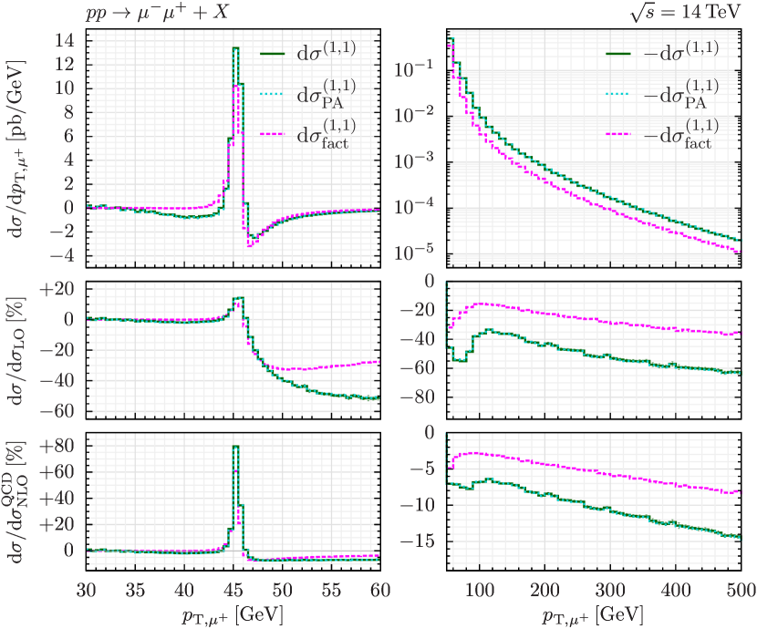
Figure 1: Complete ${\cal O}(\alpha_{\mathrm{S}}\alpha)$ correction to the differential cross section $d\sigma^{(1,1)}$ in the anti-muon $p_{T}$ compared to the corresponding result in the pole approximation and to the factorised approximation $d\sigma^{(1,1)}_{\rm fact}$. The top panels show the absolute predictions, while the central (bottom) panels display the ${\cal O}(\alpha_{\mathrm{S}}\alpha)$ correction normalized to the LO (NLO QCD) result. For the full result the ratios also display our estimate of the numerical uncertainties, obtained as described in the text.

In Fig. 1 we present our result for the ${\cal O}(\alpha_{\mathrm{S}}\alpha)$ correction as a function of the anti-muon $p_{T}$. The left panels depict the region around the $Z$ peak, and the right panels the high-$p_{T}$ region. In the main panels we show the absolute correction $d\sigma^{(1,1)}/dp_{T}$, while the central (bottom) panels display the correction normalised to the LO (NLO QCD) result. Our results for the complete ${\cal O}(\alpha_{\mathrm{S}}\alpha)$ correction are compared with those obtained in two approximations. The first approximation consists in computing the finite part of the two-loop virtual amplitude in the pole approximation, suitably reweighted with the exact squared Born amplitude. This approach precisely follows that adopted for the charged-current DY process in Ref. [49] (see Eq. (14) therein for the precise definition). The pole approximation, which includes factorisable and non-factorisable [44] contributions, requires the QCD–EW on-shell form factor of the $Z$ boson [40]. The second approximation is based on a fully factorised approach for QCD and EW corrections, where we exclude photon-induced processes throughout (see Ref. [45, 49] for a detailed description). We see that the result obtained in the pole approximation is in perfect agreement with the exact result. This is due to the small contribution of the two-loop virtual to the computed correction, as observed also in the case of $W$ production [49]. Our result for the ${\cal O}(\alpha_{\mathrm{S}}\alpha)$ correction in the region of the peak is reproduced relatively well by the factorised approximation. Beyond the Jacobian peak, this approximation tends to overshoot the complete result, which is consistent with what was observed in Refs. [45, 49]. As $p_{T}$ increases, the (negative) impact of the mixed QCD–EW corrections increases, and at $p_{T}=500$ GeV it reaches about $-60\%$ with respect to the LO prediction and $-15\%$ with respect to the NLO QCD result. The factorised approximation describes the qualitative behaviour of the complete correction reasonably well, also in the tail of the distribution, but it overshoots the full result as $p_{T}$ increases.

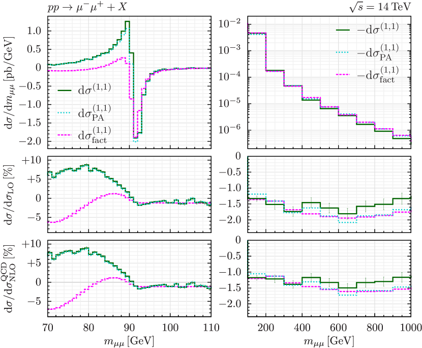
Figure 2: As Fig. 1, but for the di-muon invariant mass.

In Fig. 2 we show our result for the ${\cal O}(\alpha_{\mathrm{S}}\alpha)$ correction as a function of the di-muon invariant mass $m_{\mu\mu}$. The left panels depict the region around the $Z$ peak, and the right panels the high-$m_{\mu\mu}$ region. When comparing the factorised approximation with the exact result, we notice that it fails to describe the radiative correction below the $Z$ resonance, as already pointed out in Ref. [45]. In contrast, the pole approximation is a very good approximation of the complete correction, with some small differences that can be appreciated right around the peak. In the high-$m_{\mu\mu}$ region the correction is uniformly of the order of $-1.5\%$ with respect to the NLO QCD result. Here the trend of the negative correction is captured by both approximations, which, however, both undershoot the exact result by about $30\%$, highlighting the relevance of the exact two-loop contribution for this observable.

The numerical evaluation of the above results for $d\sigma^{(1,1)}$ (and $d\sigma^{(2,0)}$) requires the introduction of a technical cut-off $r_{\rm cut}$ on the dimensionless variable $q_{T}/m_{\mu\mu}$ in the square bracket of Eq. (3). We follow the procedure in Matrix [100] to simultaneously calculate for several values of $r_{\rm cut}$ and to perform a numerical extrapolation $r_{\rm cut}\rightarrow 0$, but apply it on a bin-wise level. Quadratic least $\chi^{2}$ fits in the range $[0.01\%,r_{\rm max}]$ with $r_{\rm max}\in[0.25\%,0.5\%]$ are used to determine best predictions and extrapolation error estimates. In the case of the anti-muon $p_{T}$ distribution, the final uncertainties of the computed correction, combining statistical and systematic errors, range from the percent level in the peak region to ${\cal O}(3\%)$ in the tail. In the case of the di-muon invariant mass, the final uncertainties are larger, and range from the few percent level in the peak region to ${\cal O}(10\%)$ at high $m_{\mu\mu}$ values.

IV Summary

In this Letter we have presented the first complete computation of the mixed QCD–EW corrections to neutral-current DY lepton pair production at the LHC. All the real and virtual contributions due to initial- and final-state radiation are included exactly, thereby allowing us to investigate the impact of the computed corrections in the entire region of dilepton invariant masses. The evaluation of the two-loop virtual amplitude has been achieved by using semi-analytical techniques. To cancel soft and collinear singularities, we have used a formulation of the $q_{T}$ subtraction formalism derived from the NNLO QCD calculation for heavy-quark production through an appropriate abelianisation procedure. Our computation is fully differential in the momenta of the charged leptons and the associated QED and QCD radiation. Therefore, it can be used to compute arbitrary infrared-safe observables, and, in particular, we can also deal with dressed leptons, i.e. leptons recombined with close-by photons. More detailed results of our calculation will be presented elsewhere.

Acknowledgements

We would like to express our gratitude to Jean-Nicolas Lang and Jonas Lindert for their continuous support on Recola and OpenLoops, to Simone Devoto for fruitful discussions and several checks of the two-loop amplitudes, and to Chiara Savoini for numerical checks of the pole approximation. This work is supported in part by the Swiss National Science Foundation (SNF) under contract 200020$\_$188464. The work of SK is supported by the ERC Starting Grant 714788 REINVENT. FT acknowledges support from INFN. AV and NR are supported by the Italian Ministero dell’Università e della Ricerca (Grant No. PRIN2017) and by the European Research Council under the European Unions Horizon 2020 research and innovation Programme (Grant Agreement No. 740006). RB and NR acknowledge the COST (European Cooperation in Science and Technology) Action CA16201 PARTICLEFACE for partial support.

References

- Aad et al. [2012] G. Aad et al. (ATLAS), Observation of a new particle in the search for the Standard Model Higgs boson with the ATLAS detector at the LHC, Phys. Lett. B 716, 1 (2012), arXiv:1207.7214 [hep-ex] .
- Chatrchyan et al. [2012] S. Chatrchyan et al. (CMS), Observation of a New Boson at a Mass of 125 GeV with the CMS Experiment at the LHC, Phys. Lett. B 716, 30 (2012), arXiv:1207.7235 [hep-ex] .
- Drell and Yan [1970] S. Drell and T.-M. Yan, Massive Lepton Pair Production in Hadron-Hadron Collisions at High-Energies, Phys. Rev. Lett. 25, 316 (1970), [Erratum: Phys.Rev.Lett. 25, 902 (1970)].
- Arnison et al. [1983a] G. Arnison et al. (UA1), Experimental Observation of Isolated Large Transverse Energy Electrons with Associated Missing Energy at GeV, Phys. Lett. B 122, 103 (1983a).
- Banner et al. [1983] M. Banner et al. (UA2), Observation of Single Isolated Electrons of High Transverse Momentum in Events with Missing Transverse Energy at the CERN anti-p p Collider, Phys. Lett. B 122, 476 (1983).
- Arnison et al. [1983b] G. Arnison et al. (UA1), Experimental Observation of Lepton Pairs of Invariant Mass Around 95-GeV/c**2 at the CERN SPS Collider, Phys. Lett. B 126, 398 (1983b).
- Bagnaia et al. [1983] P. Bagnaia et al. (UA2), Evidence for at the CERN Collider, Phys. Lett. B 129, 130 (1983).
- Group [2012] T. E. W. Group (CDF, D0), 2012 Update of the Combination of CDF and D0 Results for the Mass of the W Boson, (2012), arXiv:1204.0042 [hep-ex] .
- Aaboud et al. [2018] M. Aaboud et al. (ATLAS), Measurement of the -boson mass in pp collisions at TeV with the ATLAS detector, Eur. Phys. J. C 78, 110 (2018), [Erratum: Eur.Phys.J.C 78, 898 (2018)], arXiv:1701.07240 [hep-ex] .
- Aaltonen et al. [2018] T. A. Aaltonen et al. (CDF, D0), Tevatron Run II combination of the effective leptonic electroweak mixing angle, Phys. Rev. D 97, 112007 (2018), arXiv:1801.06283 [hep-ex] .
- ATL [2018] Measurement of the effective leptonic weak mixing angle using electron and muon pairs from -boson decay in the ATLAS experiment at TeV, ATLAS-CONF-2018-037 (2018).
- Altarelli et al. [1979] G. Altarelli, R. Ellis, and G. Martinelli, Large Perturbative Corrections to the Drell-Yan Process in QCD, Nucl. Phys. B 157, 461 (1979).
- Hamberg et al. [1991] R. Hamberg, W. van Neerven, and T. Matsuura, A complete calculation of the order correction to the Drell-Yan factor, Nucl. Phys. B 359, 343 (1991), [Erratum: Nucl.Phys.B 644, 403–404 (2002)].
- Harlander and Kilgore [2002] R. V. Harlander and W. B. Kilgore, Next-to-next-to-leading order Higgs production at hadron colliders, Phys. Rev. Lett. 88, 201801 (2002), arXiv:hep-ph/0201206 .
- Anastasiou et al. [2003] C. Anastasiou, L. J. Dixon, K. Melnikov, and F. Petriello, Dilepton rapidity distribution in the Drell-Yan process at NNLO in QCD, Phys. Rev. Lett. 91, 182002 (2003), arXiv:hep-ph/0306192 .
- Anastasiou et al. [2004] C. Anastasiou, L. J. Dixon, K. Melnikov, and F. Petriello, High precision QCD at hadron colliders: Electroweak gauge boson rapidity distributions at NNLO, Phys. Rev. D 69, 094008 (2004), arXiv:hep-ph/0312266 .
- Melnikov and Petriello [2006] K. Melnikov and F. Petriello, Electroweak gauge boson production at hadron colliders through , Phys. Rev. D 74, 114017 (2006), arXiv:hep-ph/0609070 .
- Catani et al. [2009] S. Catani, L. Cieri, G. Ferrera, D. de Florian, and M. Grazzini, Vector boson production at hadron colliders: a fully exclusive QCD calculation at NNLO, Phys. Rev. Lett. 103, 082001 (2009), arXiv:0903.2120 [hep-ph] .
- Catani et al. [2010] S. Catani, G. Ferrera, and M. Grazzini, W Boson Production at Hadron Colliders: The Lepton Charge Asymmetry in NNLO QCD, JHEP 05, 006, arXiv:1002.3115 [hep-ph] .
- Dittmaier and Krämer [2002] S. Dittmaier and M. Krämer, Electroweak radiative corrections to W boson production at hadron colliders, Phys. Rev. D 65, 073007 (2002), arXiv:hep-ph/0109062 .
- Baur and Wackeroth [2004] U. Baur and D. Wackeroth, Electroweak radiative corrections to beyond the pole approximation, Phys. Rev. D 70, 073015 (2004), arXiv:hep-ph/0405191 .
- Zykunov [2006] V. Zykunov, Radiative corrections to the Drell-Yan process at large dilepton invariant masses, Phys. Atom. Nucl. 69, 1522 (2006).
- Arbuzov et al. [2006] A. Arbuzov, D. Bardin, S. Bondarenko, P. Christova, L. Kalinovskaya, G. Nanava, and R. Sadykov, One-loop corrections to the Drell-Yan process in SANC. I. The Charged current case, Eur. Phys. J. C 46, 407 (2006), [Erratum: Eur.Phys.J.C 50, 505 (2007)], arXiv:hep-ph/0506110 .
- Carloni Calame et al. [2006] C. Carloni Calame, G. Montagna, O. Nicrosini, and A. Vicini, Precision electroweak calculation of the charged current Drell-Yan process, JHEP 12, 016, arXiv:hep-ph/0609170 .
- Baur et al. [2002] U. Baur, O. Brein, W. Hollik, C. Schappacher, and D. Wackeroth, Electroweak radiative corrections to neutral current Drell-Yan processes at hadron colliders, Phys. Rev. D 65, 033007 (2002), arXiv:hep-ph/0108274 .
- Zykunov [2007] V. Zykunov, Weak radiative corrections to Drell-Yan process for large invariant mass of di-lepton pair, Phys. Rev. D 75, 073019 (2007), arXiv:hep-ph/0509315 .
- Carloni Calame et al. [2007] C. Carloni Calame, G. Montagna, O. Nicrosini, and A. Vicini, Precision electroweak calculation of the production of a high transverse-momentum lepton pair at hadron colliders, JHEP 10, 109, arXiv:0710.1722 [hep-ph] .
- Arbuzov et al. [2008] A. Arbuzov, D. Bardin, S. Bondarenko, P. Christova, L. Kalinovskaya, G. Nanava, and R. Sadykov, One-loop corrections to the Drell–Yan process in SANC. (II). The Neutral current case, Eur. Phys. J. C 54, 451 (2008), arXiv:0711.0625 [hep-ph] .
- Dittmaier and Huber [2010] S. Dittmaier and M. Huber, Radiative corrections to the neutral-current Drell-Yan process in the Standard Model and its minimal supersymmetric extension, JHEP 01, 060, arXiv:0911.2329 [hep-ph] .
- Duhr et al. [2020a] C. Duhr, F. Dulat, and B. Mistlberger, Drell-Yan Cross Section to Third Order in the Strong Coupling Constant, Phys. Rev. Lett. 125, 172001 (2020a), arXiv:2001.07717 [hep-ph] .
- Duhr et al. [2020b] C. Duhr, F. Dulat, and B. Mistlberger, Charged current Drell-Yan production at N3LO, JHEP 11, 143, arXiv:2007.13313 [hep-ph] .
- Camarda et al. [2021] S. Camarda, L. Cieri, and G. Ferrera, Drell-Yan lepton-pair production: resummation at N3LL accuracy and fiducial cross sections at N3LO, (2021), arXiv:2103.04974 [hep-ph] .
- Barze et al. [2013] L. Barze, G. Montagna, P. Nason, O. Nicrosini, F. Piccinini, and A. Vicini, Neutral current Drell-Yan with combined QCD and electroweak corrections in the POWHEG BOX, Eur. Phys. J. C 73, 2474 (2013), arXiv:1302.4606 [hep-ph] .
- Frederix et al. [2018] R. Frederix, S. Frixione, V. Hirschi, D. Pagani, H. S. Shao, and M. Zaro, The automation of next-to-leading order electroweak calculations, JHEP 07, 185, arXiv:1804.10017 [hep-ph] .
- de Florian et al. [2018] D. de Florian, M. Der, and I. Fabre, QCDQED NNLO corrections to Drell Yan production, Phys. Rev. D 98, 094008 (2018), arXiv:1805.12214 [hep-ph] .
- Cieri et al. [2020] L. Cieri, D. de Florian, M. Der, and J. Mazzitelli, Mixed QCDQED corrections to exclusive Drell Yan production using the qT -subtraction method, JHEP 09, 155, arXiv:2005.01315 [hep-ph] .
- Delto et al. [2020] M. Delto, M. Jaquier, K. Melnikov, and R. Röntsch, Mixed QCDQED corrections to on-shell boson production at the LHC, JHEP 01, 043, arXiv:1909.08428 [hep-ph] .
- Bonciani et al. [2017] R. Bonciani, F. Buccioni, R. Mondini, and A. Vicini, Double-real corrections at to single gauge boson production, Eur. Phys. J. C 77, 187 (2017), arXiv:1611.00645 [hep-ph] .
- Bonciani et al. [2020a] R. Bonciani, F. Buccioni, N. Rana, I. Triscari, and A. Vicini, NNLO QCDEW corrections to Z production in the channel, Phys. Rev. D 101, 031301 (2020a), arXiv:1911.06200 [hep-ph] .
- Bonciani et al. [2020b] R. Bonciani, F. Buccioni, N. Rana, and A. Vicini, NNLO QCDEW corrections to on-shell production, Phys. Rev. Lett. 125, 232004 (2020b), arXiv:2007.06518 [hep-ph] .
- Buccioni et al. [2020] F. Buccioni, F. Caola, M. Delto, M. Jaquier, K. Melnikov, and R. Röntsch, Mixed QCD-electroweak corrections to on-shell Z production at the LHC, Phys. Lett. B 811, 135969 (2020), arXiv:2005.10221 [hep-ph] .
- Behring et al. [2021a] A. Behring, F. Buccioni, F. Caola, M. Delto, M. Jaquier, K. Melnikov, and R. Röntsch, Mixed QCD-electroweak corrections to -boson production in hadron collisions, Phys. Rev. D 103, 013008 (2021a), arXiv:2009.10386 [hep-ph] .
- Denner and Dittmaier [2020] A. Denner and S. Dittmaier, Electroweak Radiative Corrections for Collider Physics, Phys. Rept. 864, 1 (2020), arXiv:1912.06823 [hep-ph] .
- Dittmaier et al. [2014] S. Dittmaier, A. Huss, and C. Schwinn, Mixed QCD-electroweak corrections to Drell-Yan processes in the resonance region: pole approximation and non-factorizable corrections, Nucl. Phys. B 885, 318 (2014), arXiv:1403.3216 [hep-ph] .
- Dittmaier et al. [2016] S. Dittmaier, A. Huss, and C. Schwinn, Dominant mixed QCD-electroweak O(s) corrections to Drell–Yan processes in the resonance region, Nucl. Phys. B 904, 216 (2016), arXiv:1511.08016 [hep-ph] .
- Carloni Calame et al. [2017] C. M. Carloni Calame, M. Chiesa, H. Martinez, G. Montagna, O. Nicrosini, F. Piccinini, and A. Vicini, Precision Measurement of the W-Boson Mass: Theoretical Contributions and Uncertainties, Phys. Rev. D 96, 093005 (2017), arXiv:1612.02841 [hep-ph] .
- Behring et al. [2021b] A. Behring, F. Buccioni, F. Caola, M. Delto, M. Jaquier, K. Melnikov, and R. Röntsch, Estimating the impact of mixed QCD-electroweak corrections on the -mass determination at the LHC, Phys. Rev. D 103, 113002 (2021b), arXiv:2103.02671 [hep-ph] .
- Dittmaier et al. [2020] S. Dittmaier, T. Schmidt, and J. Schwarz, Mixed NNLO QCDelectroweak corrections of to single-W/Z production at the LHC, JHEP 12, 201, arXiv:2009.02229 [hep-ph] .
- Buonocore et al. [2021] L. Buonocore, M. Grazzini, S. Kallweit, C. Savoini, and F. Tramontano, Mixed QCD-EW corrections to at the LHC, (2021), arXiv:2102.12539 [hep-ph] .
- Bonciani et al. [2016] R. Bonciani, S. Di Vita, P. Mastrolia, and U. Schubert, Two-Loop Master Integrals for the mixed EW-QCD virtual corrections to Drell-Yan scattering, JHEP 09, 091, arXiv:1604.08581 [hep-ph] .
- Heller et al. [2020a] M. Heller, A. von Manteuffel, and R. M. Schabinger, Multiple polylogarithms with algebraic arguments and the two-loop EW-QCD Drell-Yan master integrals, Phys. Rev. D 102, 016025 (2020a), arXiv:1907.00491 [hep-th] .
- Hasan and Schubert [2020] S. M. Hasan and U. Schubert, Master Integrals for the mixed QCD-QED corrections to the Drell-Yan production of a massive lepton pair, JHEP 11, 107, arXiv:2004.14908 [hep-ph] .
- Bonciani et al. [2008] R. Bonciani, A. Ferroglia, T. Gehrmann, D. Maitre, and C. Studerus, Two-Loop Fermionic Corrections to Heavy-Quark Pair Production: The Quark-Antiquark Channel, JHEP 07, 129, arXiv:0806.2301 [hep-ph] .
- Bonciani et al. [2009] R. Bonciani, A. Ferroglia, T. Gehrmann, and C. Studerus, Two-Loop Planar Corrections to Heavy-Quark Pair Production in the Quark-Antiquark Channel, JHEP 08, 067, arXiv:0906.3671 [hep-ph] .
- Mastrolia et al. [2017] P. Mastrolia, M. Passera, A. Primo, and U. Schubert, Master integrals for the NNLO virtual corrections to scattering in QED: the planar graphs, JHEP 11, 198, arXiv:1709.07435 [hep-ph] .
- Heller et al. [2020b] M. Heller, A. von Manteuffel, R. M. Schabinger, and H. Spiesberger, Mixed EW-QCD two-loop amplitudes for and scheme independence of multi-loop corrections, (2020b), arXiv:2012.05918 [hep-ph] .
- Cascioli et al. [2012] F. Cascioli, P. Maierhöfer, and S. Pozzorini, Scattering Amplitudes with Open Loops, Phys. Rev. Lett. 108, 111601 (2012), arXiv:1111.5206 [hep-ph] .
- Buccioni et al. [2018] F. Buccioni, S. Pozzorini, and M. Zoller, On-the-fly reduction of open loops, Eur. Phys. J. C 78, 70 (2018), arXiv:1710.11452 [hep-ph] .
- Buccioni et al. [2019] F. Buccioni, J.-N. Lang, J. M. Lindert, P. Maierhöfer, S. Pozzorini, H. Zhang, and M. F. Zoller, OpenLoops 2, Eur. Phys. J. C 79, 866 (2019), arXiv:1907.13071 [hep-ph] .
- Actis et al. [2017] S. Actis, A. Denner, L. Hofer, J.-N. Lang, A. Scharf, and S. Uccirati, RECOLA: REcursive Computation of One-Loop Amplitudes, Comput. Phys. Commun. 214, 140 (2017), arXiv:1605.01090 [hep-ph] .
- Denner et al. [2018] A. Denner, J.-N. Lang, and S. Uccirati, Recola2: REcursive Computation of One-Loop Amplitudes 2, Comput. Phys. Commun. 224, 346 (2018), arXiv:1711.07388 [hep-ph] .
- Nogueira [1993] P. Nogueira, Automatic Feynman graph generation, J. Comput. Phys. 105, 279 (1993).
- Vermaseren [2000] J. A. M. Vermaseren, New features of FORM, (2000), arXiv:math-ph/0010025 .
- Kreimer [1990] D. Kreimer, The (5) Problem and Anomalies: A Clifford Algebra Approach, Phys. Lett. B 237, 59 (1990).
- Larin [1993] S. A. Larin, The Renormalization of the axial anomaly in dimensional regularization, Phys. Lett. B 303, 113 (1993), arXiv:hep-ph/9302240 .
- Tkachov [1981] F. V. Tkachov, A Theorem on Analytical Calculability of Four Loop Renormalization Group Functions, Phys. Lett. B 100, 65 (1981).
- Chetyrkin and Tkachov [1981] K. G. Chetyrkin and F. V. Tkachov, Integration by Parts: The Algorithm to Calculate beta Functions in 4 Loops, Nucl. Phys. B 192, 159 (1981).
- Gehrmann and Remiddi [2000] T. Gehrmann and E. Remiddi, Differential equations for two loop four point functions, Nucl. Phys. B580, 485 (2000), arXiv:hep-ph/9912329 [hep-ph] .
- Maierhöfer et al. [2018] P. Maierhöfer, J. Usovitsch, and P. Uwer, Kira—A Feynman integral reduction program, Comput. Phys. Commun. 230, 99 (2018), arXiv:1705.05610 [hep-ph] .
- Lee [2012] R. N. Lee, Presenting LiteRed: a tool for the Loop InTEgrals REDuction, (2012), arXiv:1212.2685 [hep-ph] .
- Studerus [2010] C. Studerus, Reduze-Feynman Integral Reduction in C++, Comput. Phys. Commun. 181, 1293 (2010), arXiv:0912.2546 [physics.comp-ph] .
- von Manteuffel and Studerus [2012] A. von Manteuffel and C. Studerus, Reduze 2 - Distributed Feynman Integral Reduction, (2012), arXiv:1201.4330 [hep-ph] .
- Goncharov [1995] A. Goncharov, Polylogarithms in arithmetic and geometry, Proceedings of the International Congree of Mathematicians 1,2, 374 (1995).
- Goncharov [2001] A. Goncharov, Multiple polylogarithms and mixed Tate motives, (2001), arXiv:math/0103059 [math.AG] .
- Remiddi and Vermaseren [2000] E. Remiddi and J. Vermaseren, Harmonic polylogarithms, Int.J.Mod.Phys. A15, 725 (2000), arXiv:hep-ph/9905237 [hep-ph] .
- Chen [1977] K.-T. Chen, Iterated path integrals, Bull. Am. Math. Soc. 83, 831 (1977).
- Moriello [2020] F. Moriello, Generalised power series expansions for the elliptic planar families of Higgs + jet production at two loops, JHEP 01, 150, arXiv:1907.13234 [hep-ph] .
- Hidding [2020] M. Hidding, DiffExp, a Mathematica package for computing Feynman integrals in terms of one-dimensional series expansions, (2020), arXiv:2006.05510 [hep-ph] .
- Smirnov [2016] A. V. Smirnov, FIESTA4: Optimized Feynman integral calculations with GPU support, Comput. Phys. Commun. 204, 189 (2016), arXiv:1511.03614 [hep-ph] .
- Borowka et al. [2018] S. Borowka, G. Heinrich, S. Jahn, S. P. Jones, M. Kerner, J. Schlenk, and T. Zirke, pySecDec: a toolbox for the numerical evaluation of multi-scale integrals, Comput. Phys. Commun. 222, 313 (2018), arXiv:1703.09692 [hep-ph] .
- Note [1] We have explicitly checked the cancellation of the collinear divergences arising in the box diagrams with a photon exchanged between the quark and lepton lines [110].
- Denner et al. [1995] A. Denner, G. Weiglein, and S. Dittmaier, Application of the background field method to the electroweak standard model, Nucl. Phys. B 440, 95 (1995), arXiv:hep-ph/9410338 .
- Sirlin [1980] A. Sirlin, Radiative Corrections in the SU(2)-L x U(1) Theory: A Simple Renormalization Framework, Phys. Rev. D22, 971 (1980).
- Degrassi and Vicini [2004] G. Degrassi and A. Vicini, Two loop renormalization of the electric charge in the standard model, Phys. Rev. D69, 073007 (2004), arXiv:hep-ph/0307122 [hep-ph] .
- Kniehl [1990] B. A. Kniehl, Two Loop Corrections to the Vacuum Polarizations in Perturbative QCD, Nucl. Phys. B 347, 86 (1990).
- Djouadi and Gambino [1994] A. Djouadi and P. Gambino, Electroweak gauge bosons selfenergies: Complete QCD corrections, Phys. Rev. D 49, 3499 (1994), [Erratum: Phys.Rev.D 53, 4111 (1996)], arXiv:hep-ph/9309298 .
- Catani and Grazzini [2007] S. Catani and M. Grazzini, An NNLO subtraction formalism in hadron collisions and its application to Higgs boson production at the LHC, Phys. Rev. Lett. 98, 222002 (2007), arXiv:hep-ph/0703012 .
- Catani et al. [2019a] S. Catani, S. Devoto, M. Grazzini, S. Kallweit, J. Mazzitelli, and H. Sargsyan, Top-quark pair hadroproduction at next-to-next-to-leading order in QCD, Phys. Rev. D 99, 051501 (2019a), arXiv:1901.04005 [hep-ph] .
- Catani et al. [2019b] S. Catani, S. Devoto, M. Grazzini, S. Kallweit, and J. Mazzitelli, Top-quark pair production at the LHC: Fully differential QCD predictions at NNLO, JHEP 07, 100, arXiv:1906.06535 [hep-ph] .
- Catani et al. [2021] S. Catani, S. Devoto, M. Grazzini, S. Kallweit, and J. Mazzitelli, Bottom-quark production at hadron colliders: fully differential predictions in NNLO QCD, JHEP 03, 029, arXiv:2010.11906 [hep-ph] .
- Buonocore et al. [2020] L. Buonocore, M. Grazzini, and F. Tramontano, The subtraction method: electroweak corrections and power suppressed contributions, Eur. Phys. J. C 80, 254 (2020), arXiv:1911.10166 [hep-ph] .
- Catani and Seymour [1996] S. Catani and M. H. Seymour, The Dipole formalism for the calculation of QCD jet cross-sections at next-to-leading order, Phys. Lett. B 378, 287 (1996), arXiv:hep-ph/9602277 .
- Catani and Seymour [1997] S. Catani and M. H. Seymour, A General algorithm for calculating jet cross-sections in NLO QCD, Nucl. Phys. B 485, 291 (1997), [Erratum: Nucl.Phys.B 510, 503–504 (1998)], arXiv:hep-ph/9605323 .
- Catani et al. [2002] S. Catani, S. Dittmaier, M. H. Seymour, and Z. Trocsanyi, The Dipole formalism for next-to-leading order QCD calculations with massive partons, Nucl. Phys. B 627, 189 (2002), arXiv:hep-ph/0201036 .
- Kallweit et al. [2017] S. Kallweit, J. M. Lindert, S. Pozzorini, and M. Schönherr, NLO QCD+EW predictions for diboson signatures at the LHC, JHEP 11, 120, arXiv:1705.00598 [hep-ph] .
- Dittmaier [2000] S. Dittmaier, A General approach to photon radiation off fermions, Nucl. Phys. B 565, 69 (2000), arXiv:hep-ph/9904440 .
- Dittmaier et al. [2008] S. Dittmaier, A. Kabelschacht, and T. Kasprzik, Polarized QED splittings of massive fermions and dipole subtraction for non-collinear-safe observables, Nucl. Phys. B 800, 146 (2008), arXiv:0802.1405 [hep-ph] .
- Gehrmann and Greiner [2010] T. Gehrmann and N. Greiner, Photon Radiation with MadDipole, JHEP 12, 050, arXiv:1011.0321 [hep-ph] .
- Schönherr [2018] M. Schönherr, An automated subtraction of NLO EW infrared divergences, Eur. Phys. J. C 78, 119 (2018), arXiv:1712.07975 [hep-ph] .
- Grazzini et al. [2018] M. Grazzini, S. Kallweit, and M. Wiesemann, Fully differential NNLO computations with MATRIX, Eur. Phys. J. C 78, 537 (2018), arXiv:1711.06631 [hep-ph] .
- Note [2] Munich, which is the abbreviation of \IeC“MUlti-chaNnel Integrator at Swiss (CH) precision\IeC”, is an automated parton-level NLO generator by S. Kallweit.
- Ablinger [2009] J. Ablinger, A Computer Algebra Toolbox for Harmonic Sums Related to Particle Physics, Master’s thesis, Linz U. (2009), arXiv:1011.1176 [math-ph] .
- Ablinger [2014] J. Ablinger, The package HarmonicSums: Computer Algebra and Analytic aspects of Nested Sums, PoS LL2014, 019 (2014), arXiv:1407.6180 [cs.SC] .
- Vollinga and Weinzierl [2005] J. Vollinga and S. Weinzierl, Numerical evaluation of multiple polylogarithms, Comput. Phys. Commun. 167, 177 (2005), arXiv:hep-ph/0410259 .
- Duhr and Dulat [2019] C. Duhr and F. Dulat, PolyLogTools — polylogs for the masses, JHEP 08, 135, arXiv:1904.07279 [hep-th] .
- Denner et al. [2005] A. Denner, S. Dittmaier, M. Roth, and L. H. Wieders, Electroweak corrections to charged-current e+ e- — 4 fermion processes: Technical details and further results, Nucl. Phys. B 724, 247 (2005), [Erratum: Nucl.Phys.B 854, 504–507 (2012)], arXiv:hep-ph/0505042 .
- Note [3] For a technical limitation of the semi-analytical approach, the evaluation of the box-type Feynman diagrams with two internal massive lines has been carried out with real masses of the gauge bosons in the Feynman integrals.
- Bertone et al. [2018] V. Bertone, S. Carrazza, N. P. Hartland, and J. Rojo (NNPDF), Illuminating the photon content of the proton within a global PDF analysis, SciPost Phys. 5, 008 (2018), arXiv:1712.07053 [hep-ph] .
- Manohar et al. [2016] A. Manohar, P. Nason, G. P. Salam, and G. Zanderighi, How bright is the proton? A precise determination of the photon parton distribution function, Phys. Rev. Lett. 117, 242002 (2016), arXiv:1607.04266 [hep-ph] .
- Frenkel and Taylor [1976] J. Frenkel and J. C. Taylor, Exponentiation of Leading Infrared Divergences in Massless Yang-Mills Theories, Nucl. Phys. B 116, 185 (1976).