Cosmological Scattering Equations

Abstract

We propose a worldsheet formula for tree-level correlation functions describing a scalar field with arbitrary mass and quartic self-interaction in de Sitter space, which is a simple model for inflationary cosmology. The correlation functions are located on the future boundary of the spacetime and are Fourier-transformed to momentum space. Our formula is supported on mass-deformed scattering equations involving conformal generators in momentum space and reduces to the CHY formula for $\phi^{4}$ amplitudes in the flat space limit. Using the global residue theorem, we verify that it reproduces the Witten diagram expansion at four and six points, and sketch the extension to $n$ points.

I Introduction

Cosmological observations suggest the Universe underwent an early inflationary phase approximately described by four-dimensional de Sitter (dS) space Guth:1980zm ; Linde:1981mu ; Albrecht:1982wi . In this scenario, correlation functions on the dS future boundary are basic cosmological observables, encoding temperature fluctuations in the cosmic microwave background and the initial conditions for structure formation Mukhanov:1981xt . These correlators can be computed using the in-in formalism Maldacena:2002vr ; Weinberg:2005vy or derived from the so-called wavefunction of the Universe Hartle:1983ai , whose coefficients can be obtained by Wick rotating boundary correlators in Anti-de Sitter space (AdS) Maldacena:2002vr ; McFadden:2009fg ; McFadden:2010vh ; Sleight:2020obc . The wavefunction coefficients are constrained by conformal Ward identities (CWI) associated with the spacetime isometries, and can therefore be treated like correlation functions of a conformal field theory (CFT) living at the boundary Strominger:2001gp ; Bzowski:2013sza ; Bzowski:2015pba . We will refer to them as cosmological correlators.

Perturbatively, cosmological correlators can be computed using Witten diagrams ending at the future boundary Liu:1998ty ; Maldacena:2011nz ; Raju:2011mp ; Raju:2012zr ; Ghosh:2014kba ; Arkani-Hamed:2015bza . In the flat space limit, they reduce to scattering amplitudes Raju:2012zr for which a wealth of computational techniques has been developed, e.g. Britto:2005fq ; Bern:1994cg ; Arkani-Hamed:2016byb . These methods have led to remarkable new formulations such as the Cachazo-He-Yuan (CHY) formulae Cachazo:2013hca ; Cachazo:2013iea ; Mason:2013sva , recasting scattering amplitudes in a vast range of quantum field theories in terms of a universal set of scattering equations. This formulation has in turn manifested many remarkable structures Cachazo:2014xea such as the double copy relating gauge and gravitational amplitudes Bern:2008qj ; Bern:2010ue .

By comparison, far less is known about cosmological correlators and the research programme for adapting flat space techniques to backgrounds with nonzero cosmological constant is still in its infancy Arkani-Hamed:2017fdk ; Rastelli:2017udc ; Caron-Huot:2017vep ; Alday:2017vkk ; Arkani-Hamed:2018kmz ; Farrow:2018yni ; Lipstein:2019mpu ; Sleight:2019hfp ; Baumann:2019oyu ; Armstrong:2020woi ; Albayrak:2020fyp ; Baumann:2020dch ; Goodhew:2020hob ; Bzowski:2020kfw ; Meltzer:2020qbr ; Melville:2021lst ; Alday:2021odx ; Jazayeri:2021fvk ; Baumann:2021fxj ; Zhou:2021gnu ; Diwakar:2021juk . Worldsheet formulas describing massless biadjoint scalars with cubic interactions in AdS were recently proposed in Eberhardt:2020ewh ; Roehrig:2020kck . Their scattering equations are written in terms of conformal generators acting on contact Witten diagrams in position space.

In this letter, we propose a worldsheet formula for cosmological correlators describing scalar fields with arbitrary mass and quartic interaction in dS, which is one of the simplest models for inflation Martin:2013tda . Our formula is based on a mathematical structure we call the cosmological scattering equations, which take a remarkably simple form in momentum space. They directly reduce to the CHY formula for $\phi^{4}$ amplitudes in the flat space limit Cachazo:2014xea . Another nontrivial aspect of our construction is the presence of differential operators in the integrand in the form of a Pfaffian. Crucially, we find there are no ordering ambiguities.

II Cosmological correlators

We work in the Poincaré patch of $(d+1)$-dimensional dS with unit radius:

$$ds^{2}=\frac{-d\eta^{2}+(dx^{i})^{2}}{\eta^{2}},$$ (1)

where $-\infty<\eta<0$ is the conformal time, and $i=1,...,d$ runs over Euclidean boundary directions. We will interchangeably use the notation $\vec{x}$ for boundary directions.

The $n$-point cosmological correlator, $\Psi_{n}$, can be treated as a CFT correlator in the future boundary, expressed in momentum space as

$$\Psi_{n}=\delta^{d}(\vec{k}_{T})\langle\mathcal{O}(\vec{k}_{1})...\mathcal{O}(\vec{k}_{n})\rangle,$$ (2)

where $\vec{k}_{T}=\vec{k}_{1}+...+\vec{k}_{n}$. We will work with scalar operators $\mathcal{O}$ of scaling dimension $\Delta$, dual to bulk scalar fields with mass

$$m^{2}=\Delta\left(d-\Delta\right).$$ (3)

The CWI for $\Psi_{n}$ can be expressed as

$$\sum_{a=1}^{n}P^{i}_{a}\Psi_{n}=\sum_{a=1}^{n}D_{a}\Psi_{n}=\sum_{a=1}^{n}K^{i}_{a}\Psi_{n}=0,$$ (4)

where $a,b,...$ are particle labels and the conformal generators in momentum space are

$$P^{i} = k^{i},$$

$$D = k^{i}\partial_{i}+(d-\Delta),$$ (5)

$$K_{i} = k_{i}\partial^{j}\partial_{j}-2k^{j}\partial_{j}\partial_{i}-2(d-\Delta)\partial_{i},$$

with $\partial_{i}=\tfrac{\partial}{\partial k^{i}}$. Rotation generators act trivially on scalar operators so we do not include them.

III Witten diagrams

Cosmological correlators admit a perturbative expansion in terms of bulk Witten diagrams ending on the future boundary. Here we take the bulk theory to be a scalar with mass $m$ and quartic self-interaction. The operators in the dual CFT have scaling dimension $\Delta$ satisfying (3).

The bulk-to-boundary propagator is

$$\mathcal{K}_{\nu}(k,\eta)=\mathcal{N}k^{\nu}\eta^{d/2}H_{\nu}(-k\eta),$$ (6)

where $\nu=\Delta-d/2$, $k=|\vec{k}|$, $H_{\nu}$ is a Hankel function of the second kind, and $\mathcal{N}$ is a normalisation that we will not explicitly need. It satisfies $(\mathcal{D}_{k}^{2}+m^{2})\mathcal{K}_{\nu}=0$, with

$$\mathcal{D}_{k}^{2}\equiv\eta^{2}\partial_{\eta}^{2}+(1-d)\eta\partial_{\eta}+\eta^{2}k^{2},$$ (7)

and can be used to compute contact diagrams as follows:

$$\mathcal{C}^{\Delta}_{n} \equiv \int\frac{d\eta}{\eta^{d+1}}U_{1,n}(\eta),$$ (8)

$$U_{1,n}(\eta) = \prod_{a=1}^{n}\mathcal{K}_{\nu}(k_{a},\eta).$$ (9)

As we will see, all tree-level Witten diagrams can be obtained from contact diagrams by acting with certain differential operators.

A central object in our analysis is the action of the operator

$$\mathcal{D}_{a}\cdot\mathcal{D}_{b}=\tfrac{1}{2}(P_{a}^{i}K_{bi}+K_{ai}P_{b}^{i})+D_{a}D_{b},$$ (10)

on the product $\mathcal{K}_{\nu}(k_{a},\eta)\mathcal{K}_{\nu}(k_{b},\eta)\equiv\mathcal{K}_{\nu}^{a}\mathcal{K}_{\nu}^{b}$. When acting on $\mathcal{K}_{\nu}$, the boundary generators in (II) can be written in terms of derivatives with respect to conformal time

$$P^{i}\mathcal{K}_{\nu} = k^{i}\mathcal{K}_{\nu},$$

$$D\mathcal{K}_{\nu} = \eta\tfrac{\partial}{\partial\eta}\mathcal{K}_{\nu},$$ (11)

$$K_{i}\mathcal{K}_{\nu} = \eta^{2}k_{i}\mathcal{K}_{\nu},$$

leading to

$$(\mathcal{D}_{a}\cdot\mathcal{D}_{b})\mathcal{K}_{\nu}^{a}\mathcal{K}_{\nu}^{b}=\eta^{2}[\partial_{\eta}\mathcal{K}_{\nu}^{a}\partial_{\eta}\mathcal{K}_{\nu}^{b}+(\vec{k}_{a}\cdot\vec{k}_{b})\mathcal{K}_{\nu}^{a}\mathcal{K}_{\nu}^{b}].$$ (12)

It is then straightforward to show that

$$\mathcal{D}_{1...p}^{2}U_{1,n} =(\mathcal{D}_{1}+\ldots+\mathcal{D}_{p})^{2}U_{1,n},$$

$$=-pm^{2}U_{1,n}+2\sum_{1\leq a<b\leq p}(\mathcal{D}_{a}\cdot\mathcal{D}_{b})U_{1,n},$$ (13)

where in the left hand side $\mathcal{D}_{1...p}^{2}$ is defined in (7) with $k=|\vec{k}_{1}+...+\vec{k}_{p}|\equiv k_{1...p}$ and $p<n$, and the right hand side is built using the boundary conformal generators in momentum space (5), satisfying $\mathcal{D}_{a}\cdot\mathcal{D}_{a}=-m^{2}$.

In practice we will encounter the inverse of boundary differential operators constructed from those in (10). Using (13), we replace them with the inverse of the bulk differential operator in (7) leading to bulk-to-bulk propagator insertions:

$$[(\mathcal{D}_{1}+\ldots+\mathcal{D}_{p})^{2}+m^{2}]^{-1}\mathcal{C}^{\Delta}_{n}=\\ \int\frac{d\eta}{\eta^{d+1}}\frac{d\tilde{\eta}}{\tilde{\eta}^{d+1}}U_{p+1,n}(\eta)G_{\nu}(k_{1...p},\eta,\tilde{\eta})U_{1,p}(\tilde{\eta}),$$ (14)

with $(\mathcal{D}_{k}^{2}+m^{2})G_{\nu}(k,\eta,\tilde{\eta})=\eta^{d+1}\delta(\eta-\tilde{\eta})$.

IV Scattering equations

In flat space, the CHY formulae express tree-level scattering amplitudes as integrals over the Riemann sphere, mapping each external leg to a puncture. The integrals then localise onto solutions of the scattering equations (SE):

$$\sum_{a\neq b}\frac{2\,k_{a}\cdot k_{b}}{\sigma_{ab}}=0,\qquad\sigma_{ab}\equiv\sigma_{a}-\sigma_{b},$$ (15)

where $\sigma_{a}$ is the holomorphic coordinate of the $a$’th puncture. Inspired by the massive scattering equations of Dolan:2013isa and the ambitwistor string formulae in AdS Eberhardt:2020ewh ; Roehrig:2020kck , we define the scattering equations in dS momentum space in terms of the following differential operators:

$$S_{a}=\sum_{b=1\atop b\neq a}^{n}\frac{2\,({\cal D}_{a}\cdot{\cal D}_{b})+\mu_{ab}}{\sigma_{ab}}\equiv\sum_{b=1\atop b\neq a}^{n}\frac{\alpha_{ab}}{\sigma_{ab}}\,\,,$$ (16)

where $\mu_{a\,a\pm 1}=-m^{2}$ modulo $n$ and zero otherwise. This mass deformation assumes canonical ordering of the external legs $\mathbb{1}_{n}=(1,2,\ldots,n)$. Different orderings are obtained by permutations.

Using the CWI in (4), we can show that

$$\sum_{a\neq b}\alpha_{ab}=0,$$ (17)

which implies that the SE have an underlying ${\rm SL}(2,\mathbb{C})$ symmetry W.in.P . It can then be used to fix the location of three punctures using a standard procedure familiar from string theory.

A generic worldsheet integral will then take the form

$$\int_{\gamma}\prod_{a=1\atop a\neq b,c,d}^{n}\text{d}\sigma_{a}\,(S_{a})^{-1}\,(\sigma_{bc}\sigma_{cd}\sigma_{db})^{2}\,\mathcal{I}_{n},$$ (18)

where the integration contour is defined by the intersection $\gamma=\bigcap_{a\neq b,c,d}\gamma_{S_{a}}$, where $\gamma_{S_{a}}$ encircles the pole where $S_{a}$ vanishes when acting on the theory-dependent integrand $\mathcal{I}_{n}$. Following similar steps to Eberhardt:2020ewh ; Roehrig:2020kck , it is possible to show that the differential operators in (16) commute, so the measure in (18) is well-defined.

V Worldsheet Formula

Using the cosmological SE defined in the previous section, we now propose a worldsheet formula for cosmological correlators describing massive $\phi^{4}$ theory in dS momentum space:

$$\Psi_{n}=\frac{\delta^{d}(\vec{k}_{T})}{(3!)^{p-1}}\!\!\sum_{\rho\in{\rm S}_{n-1}}\!\!\!{\rm sgn}_{\rho}\,\,{\cal A}(\rho(1,2,\ldots,n-1),n)\,{\cal C}^{\Delta}_{n},$$ (19)

where $n=2p\in\rm{even}$, ${\rm S}_{n-1}$ is the permutation group and

$${\cal A}(\mathbb{1}_{n})\!=\int_{\gamma}\prod^{n}_{a\neq b,c,d}\text{d}\sigma_{a}\,S_{a}^{-1}(\sigma_{bc}\sigma_{cd}\sigma_{db})^{2}\,\,{\cal I}(\mathbb{1}_{n}),$$ (20)

with

$${\cal I}(\mathbb{1}_{n})={\rm PT}(\mathbb{1}_{n})\,\,\,{\rm Pf}^{\prime}A\,\times\!\!\!\!\!\!\!\!\!\!\sum_{\{a,b\}\in cp(\mathbb{1}_{n})}\frac{{\rm sgn}(\{a,b\})}{\sigma_{a_{1}b_{1}}\cdots\sigma_{a_{p}b_{p}}}.$$ (21)

Here ${\rm PT}(\mathbb{1}_{n})=\left(\sigma_{12}\sigma_{23}...\sigma_{n1}\right)^{-1}$, $cp(\mathbb{1}_{n})$ denotes all perfect matchings that lead to connected graphs related to the ordering $(1,2,...,n)$ Cachazo:2014xea , and the reduced Pfaffian ${\rm Pf}^{\prime}A$ is given by

$${\rm Pf}^{\prime}A=\frac{(-1)^{c+d}}{\sigma_{cd}}{\rm Pf}A^{cd}_{cd},$$ (22)

where

$${\rm Pf}A^{cd}_{cd}=\frac{\epsilon^{r_{1}s_{1}\ldots r_{p-1}s_{p-1}}(A^{cd}_{cd})_{r_{1}s_{1}}\cdots(A^{cd}_{cd})_{r_{p-1}s_{p-1}}}{2^{p-1}(p-1)!}.$$ (23)

The matrix $A^{cd}_{cd}$ is obtained from the $n\times n$ matrix

$$A_{rs} =\begin{cases}\displaystyle\frac{\alpha_{rs}}{\sigma_{rs}},&r\neq s,\\ \displaystyle\leavevmode\nobreak\ \leavevmode\nobreak\ 0,&r=s,\end{cases}$$ (24)

by removing any pair of rows and columns $\{c,d\}$.

Since $[\alpha_{rs},\alpha_{pq}]=0$ for $r\neq s\neq p\neq q$, and $\sum_{a}[P_{a}^{i},\alpha_{rs}]=\sum_{a}[D_{a},\alpha_{rs}]=\sum_{a}[K_{a}^{i},\alpha_{rs}]=0$, ${\rm Pf}^{\prime}A$ is well defined and $\Psi_{n}$ satisfies the CWI.

VI Flat Space Limit

As a first test of our formula, let us check the flat space limit $E\rightarrow 0$, where $E=k_{1}+...+k_{n}$. This limit can be accessed by taking $\eta\rightarrow-\infty$ in the integrand of the correlator Raju:2012zr ; Lipstein:2019mpu . Using the asymptotic form of the bulk-to-boundary propagators,

$$\lim_{\eta\rightarrow-\infty}\mathcal{K}_{\nu}(k,\eta)\propto k_{i}^{\nu-1/2}\eta^{(d-1)/2}e^{ik\eta},$$ (25)

equation (12) leads to

$$\lim_{\eta\rightarrow-\infty}\mathcal{D}_{a}\cdot\mathcal{D}_{b}\left(\mathcal{K}_{\nu}^{a}\mathcal{K}_{\nu}^{b}\right)=\eta^{2}(k_{a}\cdot k_{b})\mathcal{K}_{\nu}^{a}\mathcal{K}_{\nu}^{b},$$ (26)

with $(k_{a}\cdot k_{b})=-k_{a}k_{b}+\vec{k}_{a}\cdot\vec{k}_{b}$. In this limit we can therefore replace $\mathcal{D}_{a}\cdot\mathcal{D}_{b}$ with $k_{a}\cdot k_{b}$ and set $m=0$ (recall that the mass is defined in units of the inverse dS radius so in the flat space limit it will vanish).

The resulting conformal time integration then gives

$$\lim_{E\rightarrow 0}\Psi_{n}\propto E^{-\left(4-d+\frac{1}{2}(d-3)n\right)}\Pi_{i=1}^{n}k_{i}^{\nu-1/2}\mathcal{A}_{n}\delta^{d}(\vec{k}_{T}),$$ (27)

where $\mathcal{A}_{n}$ is the CHY formula for massless $\phi^{4}$ amplitudes in flat space. We have only kept contributions which arise from acting with differential operators directly on bulk-to-boundary propagators, since other contributions are subleading.

VII Four points

Let us first consider the ordered correlator

$${\cal A}(\mathbb{1}_{4}){\cal C}^{\Delta}_{4}\!=\!\!\int_{\gamma}\!\text{d}\sigma_{3}(\sigma_{41}\sigma_{12}\sigma_{24})^{2}S_{3}^{-1}\frac{{\rm PT}(\mathbb{1}_{4})(-1){\rm Pf}A^{14}_{14}}{\sigma_{14}\,(\sigma_{13}\sigma_{24})}{\cal C}^{\Delta}_{4},$$ (28)

Notice that ${\cal A}(\mathbb{1}_{4})$ has a graph representation, given in Fig. 1.

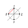
(a) ​​​​​​​​​​​​​​​​​ (b) ​​​​​​

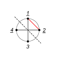
Figure 1: Factorization of ${\cal A}(\mathbb{1}_{4})$ with (a) ${\rm Pf}A^{14}_{14}$, (b) ${\rm Pf}A^{12}_{12}$.

The circle is the Parke-Taylor factor, ${\rm PT}(\mathbb{1}_{4})$, the black lines depict the perfect matching and the red line indicates the rows/columns removed from the $A$-matrix. The underlined labels $\{4,1,2\}$ are the coordinates fixed by the ${\rm SL}(2,\mathbb{C})$ symmetry. Writing $\tilde{S}_{a}=S_{a}\times\prod_{b\neq a}^{4}(\sigma_{ab})$ we obtain

$$\!\!{\cal A}(\mathbb{1}_{4})\,{\cal C}^{\Delta}_{4}=-\int_{\tilde{\gamma}}\text{d}\sigma_{3}\,\tilde{S}_{3}^{-1}\,\,\frac{\sigma_{12}\,\sigma_{24}}{\sigma_{32}}\,\alpha_{23}\,{\cal C}^{\Delta}_{4}\,,$$ (29)

where $\tilde{\gamma}$ contour is defined by $\tilde{S}_{3}$. Using the global residue theorem (GRT) Harris , $\tilde{\gamma}$ can be deformed to $\gamma_{32}$, with $\gamma_{ab}=\{|\sigma_{a}-\sigma_{b}|=\epsilon\}$. Noting that $\tilde{S}_{3}|_{\sigma_{32}=0}=\sigma_{12}\sigma_{42}\alpha_{23}$ and integrating around $\gamma_{32}$ then gives

$$\!\!{\cal A}(\mathbb{1}_{4})\,{\cal C}_{4}^{\Delta}=(\alpha_{23})^{-1}(\alpha_{23})\,\,{\cal C}_{4}^{\Delta}={\cal C}_{4}^{\Delta},$$ (30)

which is the desired result. Switching the order of the Pfaffian and the SE in (28) leads to the same expression.

When $\sigma_{3}\rightarrow\sigma_{2}$, the worldsheet factorizes into two spheres. This can be visualised by cutting the planar graph with a dotted line as shown in Fig. 1(a). On the other hand the factorizations $\sigma_{3}\rightarrow\sigma_{1}$ and $\sigma_{3}\rightarrow\sigma_{4}$ do not contribute. These observations motivate the following rules W.in.P :

1) If all fixed points (underlined labels) are on the same side of a cut then this contribution vanishes because after factorization the two new spheres must each have three fixed punctures as shown in Fig 3.

2) If a factorization cuts more than four lines in the corresponding planar graph then this contribution vanishes. For example, in Fig. 1(b) the only contribution is given by the factorization $\sigma_{3}\rightarrow\sigma_{4}$.

Because of the ${\rm SL}(2,\mathbb{C})$ symmetry, the correlator is independent of the choice of fixed punctures. These rules help to identify the most convenient choices for computations. In W.in.P , we will explicitly show that different choices are equivalent.

VIII Six points

From (20), we see that ${\cal A}(\mathbb{1}_{6})$ is encoded by the four diagrams in Fig. 2.

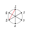
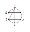
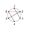
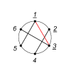
Figure 2: Diagrammatic representation of ${\cal A}(\mathbb{1}_{6})$.

In the first and second diagrams, we have fixed legs $\{5,6,1\}$ and removed the rows/columns $\{1,5\}$ from the $A$-matrix in the reduced Pfaffian. This is the simplest option. Other Pfaffian choices lead to additional contributions from the contour integrals which cancel out.

Rules 1 and 2 tell us the first diagram has only one factorization contribution, $\sigma_{3}\rightarrow\sigma_{6}$. After using the GRT we find that this diagram vanishes. The last three diagrams are identical up to cyclic permutations. We focus on the second one, i.e. ${\cal A}(\mathbb{1}_{6}:14,26,35)$, where the second argument in ${\cal A}$ denotes the perfect matching. Rules 1 and 2 imply two factorizations: $\sigma_{2}\rightarrow\sigma_{6}$ and $\sigma_{3}\rightarrow\sigma_{4}\rightarrow\sigma_{5}$. Moreover, we find that the factorization $\sigma_{2}\rightarrow\sigma_{6}$ vanishes, so the only contribution comes from the latter (Fig. 3). To compute it, we consider the parametrization $\sigma_{a}=\epsilon x_{a}+\sigma_{5}$, with $a=3,4,5$, $x_{4}=\textrm{constant}$, $x_{5}=0$, $\sigma_{5}\equiv\sigma_{L}$, and expand around $\epsilon=0$. The SE reduce to

$\Rightarrow$

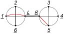
Figure 3: Factorization contribution.

$$S_{2}=[\hat{S}_{2}+{\cal O}(\epsilon)],\leavevmode\nobreak\ \hat{S}_{2}=\frac{\alpha_{21}}{\sigma_{21}}+\frac{\alpha_{26}}{\sigma_{26}}+\frac{\alpha_{2L}}{\sigma_{2L}},$$

$$S_{3}=\frac{1}{\epsilon}[\hat{S}_{3}+{\cal O}(\epsilon)],\leavevmode\nobreak\ \hat{S}_{3}=\frac{\alpha_{34}}{x_{34}}+\frac{\alpha_{35}}{x_{35}}+\frac{\alpha_{3R}}{x_{3R}},$$ (31)

$$S_{4}=\frac{1}{\epsilon}[\hat{S}_{4}+{\cal O}(\epsilon)],\leavevmode\nobreak\ \hat{S}_{4}=\frac{\alpha_{43}}{x_{43}}+\frac{\alpha_{45}}{x_{45}}+\frac{\alpha_{4R}}{x_{4R}},$$

where $x_{R}=\infty$, $\alpha_{2L}=\alpha_{23}+\alpha_{24}+\alpha_{25}$ and $\alpha_{aR}=\alpha_{a6}+\alpha_{a1}+\alpha_{a2}$, $a=3,4$. Using the GRT, the contour can then be deformed to $\hat{\gamma}=\gamma_{\epsilon}\cap\gamma_{\hat{S}_{2}}\cap\gamma_{\hat{S}_{3}}$, with $\gamma_{\epsilon}=\{|\epsilon|=\delta\}$. After performing the integral over $\epsilon$ and noting that $\hat{S}_{4}|_{\gamma_{\hat{S}_{3}}}=\frac{x_{R5}}{x_{54}\,x_{4R}}[({\cal D}_{6}+{\cal D}_{1}+{\cal D}_{2})^{2}+m^{2})]$, the remaining contour integral factorizes according to Fig. 3:

$$\!\!{\cal A}(\mathbb{1}_{6}:14,26,35)\,\,{\cal C}_{6}^{\Delta}={\cal A}(6,1,2,L:1L,26)$$

$$\!\![({\cal D}_{3}+{\cal D}_{4}+{\cal D}_{5})^{2}+m^{2}]^{-1}{\cal A}(R,3,4,5:R4,35)\,\,{\cal C}_{6}^{\Delta},$$ (32)

where

$$\!\!{\cal A}(6,1,2,L:1L,26)=$$

$$\!\!\int_{\gamma_{\hat{S}_{2}}}\!\!\!\text{d}\sigma_{2}(\sigma_{1L}\sigma_{L6}\sigma_{61})^{2}\hat{S}_{2}^{-1}{\rm PT}(6,1,2,L)\,\frac{{\rm Pf}A^{1L}_{1L}}{(\sigma_{1L}\sigma_{26})\sigma_{1L}},$$ (33)

$$\!\!{\cal A}(R,3,4,5:R4,35)=$$

$$\!\!\int_{\gamma_{\hat{S}_{3}}}\!\!\!\text{d}x_{3}(x_{45}x_{5R}x_{R4})^{2}\hat{S}_{3}^{-1}\,{\rm PT}(R,3,4,5)\,\frac{(-1){\rm Pf}A^{R5}_{R5}}{(x_{R4}x_{35})x_{R5}}.$$ (34)

Finally, using the result of the previous section we obtain

$${\cal A}(\mathbb{1}_{6}:14,26,35){\cal C}_{6}^{\Delta}\!=\![({\cal D}_{3}+{\cal D}_{4}+{\cal D}_{5})^{2}+m^{2}]^{-1}{\cal C}_{6}^{\Delta},$$ (35)

which is the Witten diagram for two 4-point vertices connected by a bulk-to-bulk propagator. Since all terms in (VIII) commute, and the scattering equations commute with Pfaffians in each four-point integrand, this implies that shuffling terms in the Pfaffian with the scattering equations in the original expression leaves the final result unchanged.

IX $n$ points

Let us briefly comment on the $n$-point computation. First notice that the six-point results can be straightforwardly extended to ladder diagrams with any number of points. In particular, let us consider the ladder diagram in Fig. 4(a), where we fix the positions of legs $\left\{n-1,n,1\right\}$ and remove rows/columns $\left\{1,n-1\right\}$ from the $A$-matrix in the reduced Pfaffian. Like in the six-point case, only one factorization contributes, notably $\sigma_{3}\rightarrow\sigma_{4}\rightarrow\cdots\rightarrow\sigma_{n-1}$.

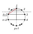
(a) ​​​​​​​ (b)

Figure 4: Factorization of (a) a ladder diagram, (b) a non-ladder diagram.

Using the parametrization, $\sigma_{a}=\epsilon x_{a}+\sigma_{n-1}$, with $a=3,4,\ldots,n-1$, $x_{n-2}=\textrm{constant}$, $x_{n-1}=0$, $\sigma_{n-1}\equiv\sigma_{L}$, and expanding around $\epsilon=0$, one obtains a generalization of (VIII):

$${\cal A}(\mathbb{1}_{n}\!:\!1(p+1),2n,...,p(p+2))\,\,{\cal C}^{\Delta}_{n}=$$

$${\cal A}(n,1,2,L:1L,2n)\,\,[({\cal D}_{n}+{\cal D}_{1}+{\cal D}_{2})^{2}+m^{2}]^{-1}\,$$

$${\cal A}(R,3,...,n-1:R(p+1),...,p(p+2))\,\,{\cal C}^{\Delta}_{n},$$ (36)

where ${\cal A}(n,1,2,L:1L,2n)$ is similar to (VIII) and

$${\cal A}(R,3,...,n-1:R(p+1),...,p(p+2))=\\ \int_{\hat{\gamma}}\prod_{a=3}^{n-3}\text{d}x_{a}\hat{S}^{-1}_{a}\frac{{\rm Pf}A^{R(n-2)}_{R(n-2)}}{x_{R(n-2)}}\\ \frac{[x_{(n-2)(n-1)}x_{(n-1)R}x_{R(n-2)}]^{2}{\rm PT}(R,...,n-1)}{(x_{R(p+1)}x_{3(n-1)}x_{4(n-2)}\cdots x_{p(p+2)})},$$ (37)

with $x_{R}=\infty$. Here we have used the identity

$$\frac{(-1){\rm Pf}A^{R(n-1)}_{R(n-1)}}{x_{R(n-1)}}=\frac{{\rm Pf}A^{R(n-2)}_{R(n-2)}}{x_{R(n-2)}}.$$ (38)

The integrand in (37) reproduces the ladder diagram of Fig. 4(a) with $(n-2)$ points, so equation (IX) provides a recursion relation. Since all terms in (IX) commute, this provides an inductive proof that we are free to shuffle terms in the Pfaffian with scattering equations, and there are no ambiguities in the definition of the integrand.

Above six points, there are graphs with other topologies as depicted in Fig.4(b). A similar procedure can be used to build up such graphs by attaching 4-point vertices to diagrams with general topology, but there are additional complications because the Pfaffian identity in (38) no longer applies W.in.P .

X Discussion

We have proposed a worldsheet description for cosmological correlators describing massive $\phi^{4}$ theory in de Sitter space. The scattering equations are written in terms of conformal generators which take a simple form in momentum space and make the flat space limit completely transparent. Another highly nontrivial ingredient of our formula is a Pfaffian defined in terms of the conformal generators.

There are a number of future directions to explore. In flat space, the scattering equations revolutionised the study of scattering amplitudes, revealing new perturbative dualities Cachazo:2014xea and providing new tools for computing loop amplitudes Geyer:2015bja ; Gomez:2017lhy ; Farrow:2020voh and soft limits Schwab:2014xua ; Adamo:2014yya ; Geyer:2014lca ; Chakrabarti:2017ltl ; Nandan:2016ohb . We therefore expect the approach developed here will lead to similar progress for cosmological correlators. Moreover, although we have focused on the simplest toy model, there are systematic ways to make it more realistic such as using more general mass deformations in order to allow fields of different masses to propagate Naculich:2014naa , considering different integrands which encode more general interactions, and breaking conformal symmetry since cosmological surveys measure correlators of curvature perturbations which become nontrivial when de Sitter boosts are broken Cheung:2007st ; Green:2020ebl ; Pajer:2020wxk . It would also be interesting to extend our formula to spinning correlators. In this case, the external polarizations introduce a bigger class of operators than the operatorial Pfaffian we consider in this paper. Moreover, it would be of great interest to directly compute correlators by diagonalising the cosmological scattering equations. While this is analytically challenging, in practice it may be numerically feasible. Our momentum space formulae may be well-suited to this purpose given their simplicity compared to those in position space.

More ambitiously, we would like to investigate how to lift of our formula to that of a UV complete theory. As a first step, we can replace the scattering equations with Koba-Nielsen factors, and Mandelstam variables with differential operators in momentum space. This may lead to ordering ambiguities similar to those encountered when lifting the Virasoro-Shapiro amplitude to AdS${}_{5}\times$ S⁵ Abl:2020dbx ; Aprile:2020mus . Ultimately, we hope that our worldsheet formula will provide a useful toy model for understanding the physics of the early Universe.

- (1) A. H. Guth, “The Inflationary Universe: A Possible Solution to the Horizon and Flatness Problems,” Phys. Rev. D 23 (1981), 347-356 doi:10.1103/PhysRevD.23.347
- (2) A. D. Linde, “A New Inflationary Universe Scenario: A Possible Solution of the Horizon, Flatness, Homogeneity, Isotropy and Primordial Monopole Problems,” Phys. Lett. B 108 (1982), 389-393 doi:10.1016/0370-2693(82)91219-9
- (3) A. Albrecht and P. J. Steinhardt, “Cosmology for Grand Unified Theories with Radiatively Induced Symmetry Breaking,” Phys. Rev. Lett. 48 (1982), 1220-1223 doi:10.1103/PhysRevLett.48.1220
- (4) V. F. Mukhanov and G. V. Chibisov, “Quantum Fluctuations and a Nonsingular Universe,” JETP Lett. 33 (1981), 532-535
- (5) J. M. Maldacena, “Non-Gaussian features of primordial fluctuations in single field inflationary models,” JHEP 05 (2003), 013 doi:10.1088/1126-6708/2003/05/013 [arXiv:astro-ph/0210603 [astro-ph]].
- (6) S. Weinberg, “Quantum contributions to cosmological correlations,” Phys. Rev. D 72 (2005), 043514 doi:10.1103/PhysRevD.72.043514 [arXiv:hep-th/0506236 [hep-th]].
- (7) J. B. Hartle and S. W. Hawking, “Wave Function of the Universe,” Phys. Rev. D 28 (1983), 2960-2975 doi:10.1103/PhysRevD.28.2960
- (8) P. McFadden and K. Skenderis, “Holography for Cosmology,” Phys. Rev. D 81 (2010), 021301 doi:10.1103/PhysRevD.81.021301 [arXiv:0907.5542 [hep-th]].
- (9) P. McFadden and K. Skenderis, “Holographic Non-Gaussianity,” JCAP 05 (2011), 013 doi:10.1088/1475-7516/2011/05/013 [arXiv:1011.0452 [hep-th]].
- (10) C. Sleight and M. Taronna, “From AdS to dS Exchanges: Spectral Representation, Mellin Amplitudes and Crossing,” [arXiv:2007.09993 [hep-th]].
- (11) A. Strominger, “Inflation and the dS / CFT correspondence,” JHEP 11 (2001), 049 doi:10.1088/1126-6708/2001/11/049 [arXiv:hep-th/0110087 [hep-th]].
- (12) A. Bzowski, P. McFadden and K. Skenderis, “Implications of conformal invariance in momentum space,” JHEP 03 (2014), 111 doi:10.1007/JHEP03(2014)111 [arXiv:1304.7760 [hep-th]].
- (13) A. Bzowski, P. McFadden and K. Skenderis, “Scalar 3-point functions in CFT: renormalisation, beta functions and anomalies,” JHEP 03 (2016), 066 doi:10.1007/JHEP03(2016)066 [arXiv:1510.08442 [hep-th]].
- (14) A. Ghosh, N. Kundu, S. Raju and S. P. Trivedi, “Conformal Invariance and the Four Point Scalar Correlator in Slow-Roll Inflation,” JHEP 07 (2014), 011 doi:10.1007/JHEP07(2014)011 [arXiv:1401.1426 [hep-th]].
- (15) H. Liu and A. A. Tseytlin, “On four point functions in the CFT / AdS correspondence,” Phys. Rev. D 59 (1999), 086002 doi:10.1103/PhysRevD.59.086002 [arXiv:hep-th/9807097 [hep-th]].
- (16) J. M. Maldacena and G. L. Pimentel, “On graviton non-Gaussianities during inflation,” JHEP 09 (2011), 045 doi:10.1007/JHEP09(2011)045 [arXiv:1104.2846 [hep-th]].
- (17) S. Raju, “Recursion Relations for AdS/CFT Correlators,” Phys. Rev. D 83 (2011), 126002 doi:10.1103/PhysRevD.83.126002 [arXiv:1102.4724 [hep-th]].
- (18) S. Raju, “New Recursion Relations and a Flat Space Limit for AdS/CFT Correlators,” Phys. Rev. D 85 (2012), 126009 doi:10.1103/PhysRevD.85.126009 [arXiv:1201.6449 [hep-th]].
- (19) N. Arkani-Hamed and J. Maldacena, “Cosmological Collider Physics,” [arXiv:1503.08043 [hep-th]].
- (20) R. Britto, F. Cachazo, B. Feng and E. Witten, “Direct proof of tree-level recursion relation in Yang-Mills theory,” Phys. Rev. Lett. 94 (2005), 181602 doi:10.1103/PhysRevLett.94.181602 [arXiv:hep-th/0501052 [hep-th]].
- (21) Z. Bern, L. J. Dixon, D. C. Dunbar and D. A. Kosower, “Fusing gauge theory tree amplitudes into loop amplitudes,” Nucl. Phys. B 435 (1995), 59-101 doi:10.1016/0550-3213(94)00488-Z [arXiv:hep-ph/9409265 [hep-ph]].
- (22) N. Arkani-Hamed, J. L. Bourjaily, F. Cachazo, A. B. Goncharov, A. Postnikov and J. Trnka, “Grassmannian Geometry of Scattering Amplitudes,” doi:10.1017/CBO9781316091548 [arXiv:1212.5605 [hep-th]].
- (23) F. Cachazo, S. He and E. Y. Yuan, “Scattering of Massless Particles in Arbitrary Dimensions,” Phys. Rev. Lett. 113 (2014) no.17, 171601 doi:10.1103/PhysRevLett.113.171601 [arXiv:1307.2199 [hep-th]].
- (24) F. Cachazo, S. He and E. Y. Yuan, “Scattering of Massless Particles: Scalars, Gluons and Gravitons,” JHEP 1407 (2014) 033 doi:10.1007/JHEP07(2014)033 [arXiv:1309.0885 [hep-th]].
- (25) L. Mason and D. Skinner, “Ambitwistor strings and the scattering equations,” JHEP 07 (2014), 048 doi:10.1007/JHEP07(2014)048 [arXiv:1311.2564 [hep-th]].
- (26) F. Cachazo, S. He and E. Y. Yuan, “Scattering Equations and Matrices: From Einstein To Yang-Mills, DBI and NLSM,” JHEP 07 (2015), 149 doi:10.1007/JHEP07(2015)149 [arXiv:1412.3479 [hep-th]].
- (27) Z. Bern, J. J. M. Carrasco and H. Johansson, “New Relations for Gauge-Theory Amplitudes,” Phys. Rev. D 78 (2008), 085011 doi:10.1103/PhysRevD.78.085011 [arXiv:0805.3993 [hep-ph]].
- (28) Z. Bern, J. J. M. Carrasco and H. Johansson, “Perturbative Quantum Gravity as a Double Copy of Gauge Theory,” Phys. Rev. Lett. 105 (2010), 061602 doi:10.1103/PhysRevLett.105.061602 [arXiv:1004.0476 [hep-th]].
- (29) N. Arkani-Hamed, P. Benincasa and A. Postnikov, “Cosmological Polytopes and the Wavefunction of the Universe,” [arXiv:1709.02813 [hep-th]].
- (30) L. Rastelli and X. Zhou, “How to Succeed at Holographic Correlators Without Really Trying,” JHEP 04 (2018), 014 doi:10.1007/JHEP04(2018)014 [arXiv:1710.05923 [hep-th]].
- (31) S. Caron-Huot, “Analyticity in Spin in Conformal Theories,” JHEP 09 (2017), 078 doi:10.1007/JHEP09(2017)078 [arXiv:1703.00278 [hep-th]].
- (32) L. F. Alday and S. Caron-Huot, “Gravitational S-matrix from CFT dispersion relations,” JHEP 12 (2018), 017 doi:10.1007/JHEP12(2018)017 [arXiv:1711.02031 [hep-th]].
- (33) J. A. Farrow, A. E. Lipstein and P. McFadden, “Double copy structure of CFT correlators,” JHEP 02 (2019), 130 doi:10.1007/JHEP02(2019)130 [arXiv:1812.11129 [hep-th]].
- (34) N. Arkani-Hamed, D. Baumann, H. Lee and G. L. Pimentel, “The Cosmological Bootstrap: Inflationary Correlators from Symmetries and Singularities,” JHEP 04 (2020), 105 doi:10.1007/JHEP04(2020)105 [arXiv:1811.00024 [hep-th]].
- (35) D. Baumann, C. Duaso Pueyo, A. Joyce, H. Lee and G. L. Pimentel, “The cosmological bootstrap: weight-shifting operators and scalar seeds,” JHEP 12 (2020), 204 doi:10.1007/JHEP12(2020)204 [arXiv:1910.14051 [hep-th]].
- (36) A. E. Lipstein and P. McFadden, “Double copy structure and the flat space limit of conformal correlators in even dimensions,” Phys. Rev. D 101 (2020) no.12, 125006 doi:10.1103/PhysRevD.101.125006 [arXiv:1912.10046 [hep-th]].
- (37) C. Sleight and M. Taronna, “Bootstrapping Inflationary Correlators in Mellin Space,” JHEP 02 (2020), 098 doi:10.1007/JHEP02(2020)098 [arXiv:1907.01143 [hep-th]].
- (38) D. Meltzer and A. Sivaramakrishnan, “CFT unitarity and the AdS Cutkosky rules,” JHEP 11 (2020), 073 doi:10.1007/JHEP11(2020)073 [arXiv:2008.11730 [hep-th]].
- (39) H. Goodhew, S. Jazayeri and E. Pajer, “The Cosmological Optical Theorem,” JCAP 04 (2021), 021 doi:10.1088/1475-7516/2021/04/021 [arXiv:2009.02898 [hep-th]].
- (40) C. Armstrong, A. E. Lipstein and J. Mei, “Color/kinematics duality in AdS4,” JHEP 02 (2021), 194 doi:10.1007/JHEP02(2021)194 [arXiv:2012.02059 [hep-th]].
- (41) S. Albayrak, S. Kharel and D. Meltzer, “On duality of color and kinematics in (A)dS momentum space,” JHEP 03 (2021), 249
- (42) D. Baumann, C. Duaso Pueyo, A. Joyce, H. Lee and G. L. Pimentel, “The Cosmological Bootstrap: Spinning Correlators from Symmetries and Factorization,” [arXiv:2005.04234 [hep-th]].
- (43) A. Bzowski, P. McFadden and K. Skenderis, “Conformal correlators as simplex integrals in momentum space,” JHEP 01 (2021), 192 doi:10.1007/JHEP01(2021)192 [arXiv:2008.07543 [hep-th]].
- (44) S. Melville and E. Pajer, “Cosmological Cutting Rules,” JHEP 05 (2021), 249 doi:10.1007/JHEP05(2021)249 [arXiv:2103.09832 [hep-th]].
- (45) L. F. Alday, C. Behan, P. Ferrero and X. Zhou, “Gluon Scattering in AdS from CFT,” JHEP 06 (2021), 020 doi:10.1007/JHEP06(2021)020 [arXiv:2103.15830 [hep-th]].
- (46) S. Jazayeri, E. Pajer and D. Stefanyszyn, “From Locality and Unitarity to Cosmological Correlators,” [arXiv:2103.08649 [hep-th]].
- (47) D. Baumann, W. M. Chen, C. Duaso Pueyo, A. Joyce, H. Lee and G. L. Pimentel, “Linking the Singularities of Cosmological Correlators,” [arXiv:2106.05294 [hep-th]].
- (48) X. Zhou, “Double Copy Relation for AdS,” [arXiv:2106.07651 [hep-th]].
- (49) P. Diwakar, A. Herderschee, R. Roiban and F. Teng, “BCJ Amplitude Relations for Anti-de Sitter Boundary Correlators in Embedding Space,” [arXiv:2106.10822 [hep-th]].
- (50) L. Eberhardt, S. Komatsu and S. Mizera, “Scattering equations in AdS: scalar correlators in arbitrary dimensions,” JHEP 11 (2020), 158 doi:10.1007/JHEP11(2020)158 [arXiv:2007.06574 [hep-th]].
- (51) K. Roehrig and D. Skinner, “Ambitwistor Strings and the Scattering Equations on AdSS3,” [arXiv:2007.07234 [hep-th]].
- (52) J. Martin, C. Ringeval and V. Vennin, “Encyclopædia Inflationaris,” Phys. Dark Univ. 5-6 (2014), 75-235 doi:10.1016/j.dark.2014.01.003 [arXiv:1303.3787 [astro-ph.CO]].
- (53) L. Dolan and P. Goddard, “Proof of the Formula of Cachazo, He and Yuan for Yang-Mills Tree Amplitudes in Arbitrary Dimension,” JHEP 1405 (2014) 010 doi:10.1007/JHEP05(2014)010 [arXiv:1311.5200 [hep-th]].
- (54) H. Gomez, A. Lipstein, R. L. Jusinskas, to appear.
- (55) P. Griffiths, J. Harris, “Principles of algebraic geometry," John Wiley Sons, New York U.S.A, 1978.
- (56) Y. Geyer, L. Mason, R. Monteiro and P. Tourkine, “Loop Integrands for Scattering Amplitudes from the Riemann Sphere,” Phys. Rev. Lett. 115 (2015) no.12, 121603 doi:10.1103/PhysRevLett.115.121603 [arXiv:1507.00321 [hep-th]].
- (57) H. Gomez, “Quadratic Feynman Loop Integrands From Massless Scattering Equations,” Phys. Rev. D 95 (2017) no.10, 106006 doi:10.1103/PhysRevD.95.106006 [arXiv:1703.04714 [hep-th]].
- (58) J. A. Farrow, Y. Geyer, A. E. Lipstein, R. Monteiro and R. Stark-Muchão, “Propagators, BCFW recursion and new scattering equations at one loop,” JHEP 10 (2020), 074 doi:10.1007/JHEP10(2020)074 [arXiv:2007.00623 [hep-th]].
- (59) B. U. W. Schwab and A. Volovich, “Subleading Soft Theorem in Arbitrary Dimensions from Scattering Equations,” Phys. Rev. Lett. 113 (2014) no.10, 101601 doi:10.1103/PhysRevLett.113.101601 [arXiv:1404.7749 [hep-th]].
- (60) T. Adamo, E. Casali and D. Skinner, “Perturbative gravity at null infinity,” Class. Quant. Grav. 31 (2014) no.22, 225008 doi:10.1088/0264-9381/31/22/225008 [arXiv:1405.5122 [hep-th]].
- (61) Y. Geyer, A. E. Lipstein and L. Mason, “Ambitwistor strings at null infinity and (subleading) soft limits,” Class. Quant. Grav. 32 (2015) no.5, 055003 doi:10.1088/0264-9381/32/5/055003 [arXiv:1406.1462 [hep-th]].
- (62) S. Chakrabarti, S. P. Kashyap, B. Sahoo, A. Sen and M. Verma, “Subleading Soft Theorem for Multiple Soft Gravitons,” JHEP 12 (2017), 150 doi:10.1007/JHEP12(2017)150 [arXiv:1707.06803 [hep-th]].
- (63) D. Nandan, J. Plefka and W. Wormsbecher, “Collinear limits beyond the leading order from the scattering equations,” JHEP 02, 038 (2017) doi:10.1007/JHEP02(2017)038 [arXiv:1608.04730 [hep-th]].
- (64) S. G. Naculich, “Scattering equations and BCJ relations for gauge and gravitational amplitudes with massive scalar particles,” JHEP 09 (2014), 029 doi:10.1007/JHEP09(2014)029 [arXiv:1407.7836 [hep-th]].
- (65) C. Cheung, P. Creminelli, A. L. Fitzpatrick, J. Kaplan and L. Senatore, “The Effective Field Theory of Inflation,” JHEP 03 (2008), 014 doi:10.1088/1126-6708/2008/03/014 [arXiv:0709.0293 [hep-th]].
- (66) D. Green and E. Pajer, “On the Symmetries of Cosmological Perturbations,” JCAP 09 (2020), 032 doi:10.1088/1475-7516/2020/09/032 [arXiv:2004.09587 [hep-th]].
- (67) E. Pajer, “Building a Boostless Bootstrap for the Bispectrum,” JCAP 01 (2021), 023 doi:10.1088/1475-7516/2021/01/023 [arXiv:2010.12818 [hep-th]].
- (68) T. Abl, P. Heslop and A. E. Lipstein, “Towards the Virasoro-Shapiro amplitude in AdS,” JHEP 04 (2021), 237 doi:10.1007/JHEP04(2021)237 [arXiv:2012.12091 [hep-th]].
- (69) F. Aprile, J. M. Drummond, H. Paul and M. Santagata, “The Virasoro-Shapiro amplitude in AdSS5 and level splitting of 10d conformal symmetry,” [arXiv:2012.12092 [hep-th]].