Comparing fermionic superfluids in two and three dimensions

Understanding the origins of unconventional superconductivity has been a major focus of condensed matter physics for many decades. While many questions remain unanswered, experiments have found that the systems with the highest critical temperatures tend to be layered materials where superconductivity occurs in two-dimensional (2D) structures Keimer et al. (2015); Ge et al. (2015); Yu et al. (2019). However, to what extent the remarkable stability of these strongly correlated 2D superfluids is related to their reduced dimensionality is still an open question Yu et al. (2019). In this work, we use dilute gases of ultracold fermionic atoms Bloch et al. (2008); Ketterle and Zwierlein (2008) as a model system to directly observe the influence of dimensionality on strongly interacting fermionic superfluids. We achieve this by measuring the superfluid gap of a strongly correlated quasi-2D Fermi gas Levinsen and Parish (2015); Turlapov and Yu Kagan (2017) over a wide range of interaction strengths and comparing the results to recent measurements in 3D Fermi gases Biss et al. (2021). We find that the superfluid gap follows the same universal function of the interaction strength in both systems, which suggests that there is no inherent difference in the stability of fermionic superfluidity between two- and three-dimensional quantum gases. Finally, we compare our data to results from solid state systems and find a similar relation between the interaction strength and the gap for a wide range of two- and three-dimensional superconductors.

Fermionic particles such as the electrons in superconductors have half-integer spin and therefore obey the Pauli exclusion principle. This prevents systems of noninteracting fermions from condensing into a macroscopic wavefunction and becoming superfluid. However, in the presence of an effective attractive interaction it can become energetically favorable for fermions with opposite spin to form bosonic pairs. These pairs can then condense into a coherent many-body state and become superfluid, as laid out by Bardeen, Cooper and Schrieffer (BCS) in their famous theory of superconductivity Bardeen et al. (1957). The energy that is required to break one of these pairs is called the superfluid gap $\Delta$, as the pairing manifests itself as a gap in the excitation spectrum of fermionic superfluids. Since breaking the pairs destroys the superfluid, the size of this gap determines the stability of the superfluid and sets its critical temperature.

Over the last decades, new classes of superconductors have been discovered that exhibit higher critical temperatures and stronger interactions than conventional BCS superconductors Uemura et al. (1991a). Of particular interest are systems where superfluidity occurs in two-dimensional structures, as they are the ones where the highest ambient-pressure critical temperatures have been observed Keimer et al. (2015). However, the dimensionality of these systems cannot be changed without dramatically altering their other properties as well, and it is therefore unclear to what extent the surprising stability of their superfluidity is predicated on their two-dimensional nature.

In this work, we directly observe the effect of reduced dimensionality on the stability of strongly interacting fermionic superfluids. We measure the superfluid gap of an ultracold 2D Fermi gas as a function of interaction strength and compare the results with our recent measurement of the gap in a three-dimensional system Biss et al. (2021). We find that the superfluid gap follows the same universal function of the chemical potential in both systems, which suggests that dimensionality has only limited influence on the stability of strongly interacting fermionic superfluids.

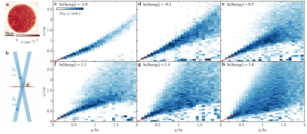
Figure 1: Excitation spectrum of a 2D Fermi gas in the BEC-BCS crossover. a: Absorption image showing the density $n(\vec{r})$ of our homogeneous 2D Fermi gas. b: Sketch of the experimental setup for measuring the excitation spectrum of our system. Two far-detuned laser beams drive a two-photon transition with energy and momentum transfer $\hbar\omega=\hbar(\omega_{1}-\omega_{2})$ and $\hbar q=\hbar|\vec{k}_{1}-\vec{k}_{2}|$, and the dynamic structure factor $S(q,\omega)$ can be obtained from the resulting heating rate. c-h: Measurements of $S(q,\omega)$ taken at different values of the 2D interaction parameter $\rm{ln}(k_{\rm F}a_{\rm 2D})$. For strong attractive interactions (c), the system consists of tightly bound molecules which are excited as unbroken pairs, and consequently $S(q,\omega)$ shows the Bogoliubov dispersion of an interacting Bose gas. Moving into the crossover regime (d,e,f), the pairs become more weakly bound and pair breaking excitations begin to appear at higher momenta. These excitations become more pronounced as we approach the BCS limit where the system shows the expected broad pair breaking continuum (g,h). In addition to these pair breaking excitations, it is also possible to excite sound waves in the superfluid. These appear in our spectra as a linear mode at low momenta, with a slope that corresponds to the speed of sound in the system and is in excellent agreement with previous measurements (red lines in panels c-h, Bohlen et al. (2020)). The data in panel a (c-h) was obtained by averaging over 26 (3-8) individual measurements. The behavior observed in (c-h) closely resembles results obtained in 3D Fermi gases Biss et al. (2021) (for a comparison see Supplementary Materials).

For our experiments, we use ultracold atomic Fermi gases of ⁶Li atoms. Such gases have two key advantages that make them uniquely suited for performing experiments that isolate the effect of dimensionality on the stability of superfluids: The first is that they are systems with simple and well-understood interparticle interactions that can be easily tuned using Feshbach resonances Chin et al. (2010). The second is that the dimensionality of the system can be controlled freely by changing the shape of the confining potential Martiyanov et al. (2010); Fröhlich et al. (2011); Sommer et al. (2012); Ries et al. (2015); Cheng et al. (2016); Mitra et al. (2016); Peppler et al. (2018); Hueck et al. (2018). By combining these two features, we can create two- and three-dimensional systems that have the same microscopic physics but different dimensionality.

To perform a quantitative comparison between these systems, we examine the effect of the reduced dimensionality on the superfluid gap. The gap is well suited for this purpose, as it directly determines both the critical current and the critical temperature of a fermionic superfluid and thus constitutes an excellent measure for its stability. As reliable measurements of the gap are available for three-dimensional Fermi gases Schirotzek et al. (2008); Hoinka et al. (2017); Biss et al. (2021), we can focus our experiments on measuring the gap in two-dimensional systems.

To bring our system into the two-dimensional regime, we apply a strong confining potential along one direction such that the chemical potential and temperature are well below the level spacing. This strongly suppresses all excitations in this direction and thereby creates an effective (or quasi-) 2D system Petrov and Shlyapnikov (2001); Levinsen and Parish (2015); Turlapov and Yu Kagan (2017) (see Supplementary Materials).

We then measure the excitation spectrum of the gas to determine the size of the superfluid gap. We use momentum resolved Bragg spectroscopy to measure the dynamic structure factor $S(q,\omega)$ of the superfluid, which describes the probability of creating an excitation in the system by providing an energy and momentum transfer of $\hbar\omega$ and $\hbar q$ (Fig. 1b, see Supplementary Materials). By tuning the strength of the interparticle interactions, we can perform such measurements throughout the crossover from a BCS superfluid of weakly bound Cooper pairs to a Bose-Einstein-condensate (BEC) of deeply bound molecules, where the interaction strength can be parametrized by the 2D interaction parameter $\rm{ln}(k_{\rm F}a_{\rm 2D})$. Here, $a_{\rm 2D}$ is the 2D scattering length Petrov and Shlyapnikov (2001), $k_{\rm F}=\sqrt{2mE_{\rm F}}/\hbar$ is the Fermi wavevector, $E_{\rm F}=\hbar\omega_{\rm F}$ is the Fermi energy, and $m$ is the mass of a ⁶Li atom.

The results of these measurements are shown in Fig. 1c-h. We observe two different types of excitations : The first are longer-range collective excitations of the superfluid, which are visible as a linear sound mode at low momentum transfers ($q\ll k_{\rm F}$), with a slope that is in excellent agreement with the speed of sound measured in Bohlen et al. (2020) (red lines in Fig. 1 c-h). This is the Goldstone mode of the system, which arises from the breaking of the U(1) symmetry of the system when the gas condenses into a superfluid Goldstone (1961); Hoinka et al. (2017). The second type of excitations are single-particle excitations that break a pair. As this process is only possible if the energy transfer is sufficiently high to overcome the energy gained from pairing, these excitations show a sharp onset at an energy transfer of $2\Delta$. This behavior is most apparent for BCS superfluids with weak attractive interactions (Fig. 1 g,h), where a pronounced continuum of pair breaking excitations is clearly visible. When increasing the interparticle attraction, the size of the superfluid gap increases and consequently the onset of the pair breaking continuum shifts towards higher energies. Additionally, as the pairs are transformed from weakly bound Cooper pairs to tightly bound bosonic molecules, the onset of the pair breaking continuum moves towards higher momenta as pair breaking excitations are suppressed when the size of the pairs becomes small compared to the length scale of the perturbation Leggett (1998); Büchler et al. (2004). This trend continues into the BEC regime, where the molecules are so tightly bound that pair breaking excitations become completely suppressed. The excitation spectrum then exhibits the well-known Bogoliubov dispersion relation of a superfluid Bose gas, which consists of a linear dispersion of phonons at low momentum and single-particle excitations of bosonic molecules at higher momenta (see Fig. 1 c).

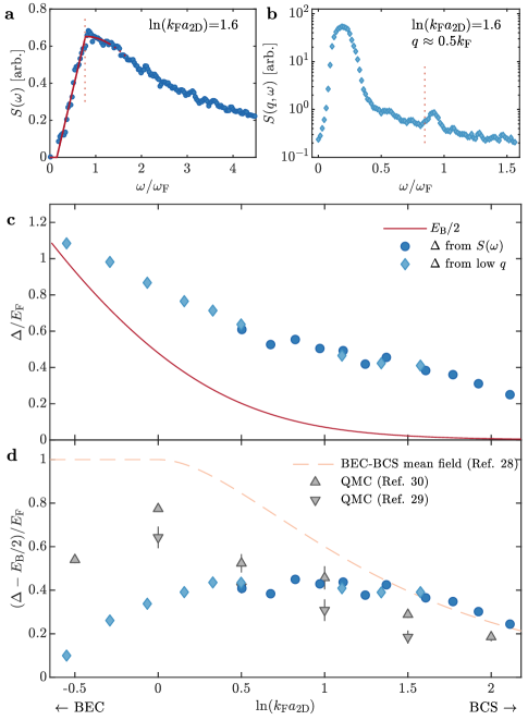
Figure 2: Superfluid gap in the 2D BEC-BCS crossover. a: Integrated dynamic structure factor $S(\omega)=\int S(q,\omega)q\,dq$ at an interaction strength of $\rm{ln}(k_{\rm F}a_{\rm 2D})=1.6$. We determine the energy $2\Delta$ (red dotted line) at which pair breaking excitations become possible from a phenomenological fit (solid red line) to $S(\omega)$ (see Supplementary Materials). b: Dynamic structure factor $S(q,\omega)$ measured at a fixed momentum transfer of $q=0.5\,k_{\rm F}$. At these small wavevectors, pair breaking is suppressed and strong driving is required to observe the onset of the pair breaking mode at $2\Delta$ (red dotted line), which causes a strong saturation of the low-energy phononic mode. c: Measured superfluid gap $\Delta$ as a function of the interaction strength. The different symbols distinguish results obtained using the approaches shown in panel a ($S(\omega)$, blue dots) and b (low $q$, light blue diamonds). The contribution of the two-body bound state to the gap is shown as a dark red line. d: Many-body contribution $\Delta-E_{\rm B}/2$ to the superfluid gap $\Delta$. BEC-BCS mean field predictions (dashed orange line, Randeria et al. (1989)) are in agreement with our measurement in the BCS regime, but deviate in the strongly correlated crossover regime. Quantum Monte-Carlo calculations (gray triangles, Vitali et al. (2017); Zielinski et al. (2020)) show better agreement in the crossover, but still deviate from the measurements in the BEC regime. Error bars denote $1\sigma$ confidence intervals of the fit and are smaller than the symbol size, the data shown in panels a (b) is the average of 8 (26) individual measurements.

To determine the superfluid gap $\Delta$ from our measurements, we integrate the measured dynamic structure factors over the momentum axis. The resulting quantity $S(\omega)=\int S(q,\omega)q\,dq$ describes the probability of creating an excitation with a given energy $\hbar\omega$ and is similar to the Raman response measured in inelastic Raman scattering experiments in solid state physics Devereaux and Hackl (2007). On the BCS side of the crossover, our measurements of $S(\omega)$ show the same behavior as observed in the Raman response of s-wave BCS superconductors: A sharp increase at $2\Delta$, followed by a slow decay back to zero Klein and Dierker (1984) (Fig. 2a). In the BCS regime, we can therefore directly extract the size of the superfluid gap from $S(\omega)$ (see Supplementary Materials).

Towards the BEC regime, extracting quantitative information from $S(\omega)$ becomes more difficult as the onset of the pair breaking continuum is masked by an increasing weight of the Goldstone mode. Fortunately, we can circumvent this problem by probing the system at lower momenta, where the energy of phononic excitations is significantly below $2\Delta$ Hoinka et al. (2017); Biss et al. (2021). While pair breaking excitations are suppressed at these low wavevectors, they can still be observed when using a stronger drive. This is shown in Fig. 2b, where the onset of the pair breaking mode at $2\Delta$ is clearly separated from the strongly driven Goldstone mode visible at lower energy. Employing both of these methods enables us to measure the superfluid gap $\Delta$ throughout the BEC-BCS crossover. The resulting values are plotted as a function of the 2D interaction parameter $\rm{ln}(k_{\rm F}a_{\rm 2D})$ in Fig. 2c, together with the binding energy $E_{\rm B}$ of the bare two-body bound state (red line), which in 2D systems exists for any non-zero attractive interaction Levinsen and Parish (2015). For our smaller attractive interactions ($\rm{ln}(k_{\rm F}a_{\rm 2D})\gtrsim 1.5$), the two-body binding energy is negligible, and the sizable gap of $\Delta\approx 0.3\,E_{\rm F}$ is entirely due to many-body effects. However, when going into the crossover regime, the trivial two-body binding energy increases and becomes comparable to the effect of the many-body BCS pairing. To separate these two contributions to the gap and thereby determine the evolution of the many-body contribution throughout the crossover, we subtract the known value of the two-body binding energy Levinsen and Parish (2015) from our measured gaps. As can be seen in Fig. 2d, the many-body contribution $\Delta-E_{\rm B}/2$ grows with increasing interactions in the BCS regime, reaches a maximum in the crossover regime and then decreases again towards the BEC side of the resonance, where the contribution of the two-body bound state begins to dominate as the gas turns into a BEC of deeply bound molecules. When comparing these results to theory, we find that they are in excellent agreement with mean-field theory Randeria et al. (1989) in the BCS regime, but begin to deviate from the mean-field results in the strongly correlated crossover region ($\rm{ln}(k_{\rm F}a_{\rm 2D})\approx 1$). Quantum Monte-Carlo (QMC) simulations Vitali et al. (2017); Zielinski et al. (2020) are in somewhat better agreement with our data in the crossover, but still predict larger values of $\Delta-E_{\rm B}/2$ in the BEC regime.

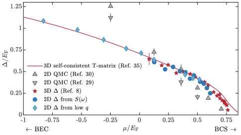
Figure 3: Comparing the gap of two-dimensional and three-dimensional superfluids. Superfluid gap $\Delta/E_{\rm F}$ of two-dimensional (blue circles and diamonds) and three-dimensional (red stars) Fermi gases as a function of the chemical potential $\mu/E_{\rm F}$, for which we use the results of QMC calculations Astrakharchik et al. (2004); Shi et al. (2015). The measurements of the gap collapse onto a single curve, which is well-described by theoretical predictions for the gap in three-dimensional Fermi gases (red line Haussmann et al. (2007); Not ); results from 2D QMC calculations Vitali et al. (2017); Zielinski et al. (2020) are shown as gray diamonds (see Supplementary Materials). Error bars denote $1\sigma$ confidence intervals of the fit.

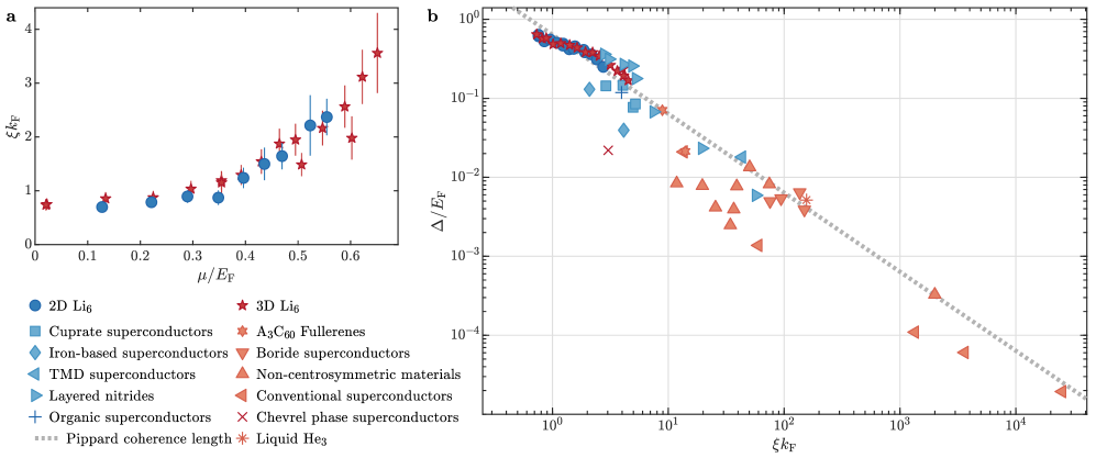
Figure 4: Fermionic superfluidity in different materials. a: Dimensionless pair size $\xi k_{\rm F}$ plotted as a function of the dimensionless chemical potential $\mu/E_{\rm F}$. As $\xi k_{\rm F}$ follows the same function of $\mu/E_{\rm F}$ for the two- and three-dimensional systems, $\xi k_{\rm F}$ can be used as an alternative parametrization of the interaction strength in our strongly interacting Fermi gases. Error bars denote $1\sigma$ confidence intervals. b: Plot of the dimensionless gap $\Delta/E_{\rm F}$ against the dimensionless pair size $\xi k_{\rm F}$ for different fermionic superfluids. The Pippard coherence length $\xi_{p}=\frac{\hbar^{2}k_{\rm F}}{\pi m\Delta}$ Ashcroft and Mermin (1976) is shown as a dotted line. Remarkably, the superfluid gap is roughly proportional to the inverse of the dimensionless pair size for a wide range of materials which span five orders of magnitude in $\Delta/E_{\rm F}$ and $\xi k_{\rm F}$. This observation applies equally to two- and three-dimensional systems, which suggests that strong correlations are more important for the stability of fermionic superfluids than the dimensionality of the system.

We now proceed to compare our measurements to recent results from 3D Fermi gases. To perform such a comparison, we need to find a suitable parametrization of the interaction strength, as the dimensionless interaction parameters $\rm{ln}(k_{\rm F}a_{\rm 2D})$ and $1/k_{\rm F}a_{\rm 3D}$ that are commonly used in two- and three-dimensional systems parametrize the interactions differently and cannot be compared directly. Instead, we parametrize the interaction strength with the normalized chemical potential $\mu/E_{\rm F}$ of the fermions. This choice is motivated by the fact that the chemical potential is a basic thermodynamic quantity that is defined independent of dimensionality and has monotonous and well-known relations to the 2D and 3D interaction parameters $\rm{ln}(k_{\rm F}a_{\rm 2D})$ and $1/k_{\rm F}a_{\rm 3D}$ Shi et al. (2015); Boettcher et al. (2016); Astrakharchik et al. (2004); Ku et al. (2012). Therefore, we can perform our comparison by plotting the superfluid gap $\Delta/E_{\rm F}$ as a function of the chemical potential $\mu/E_{\rm F}$ for two- and three-dimensional systems. The results are shown in Fig. 3.

Remarkably, we find that within the accuracy of our measurements, the results for $\Delta/E_{\rm F}$ obtained in two- and three-dimensional systems collapse onto a single curve. This suggests that for strongly interacting Fermi gases, the gap follows a single, universal function $f(\mu/E_{\rm F})=\Delta/E_{\rm F}$ of the interaction strength that is independent of the dimensionality of the system. The data appears to be well-described by theoretical predictions for three-dimensional fermionic superfluids Haussmann et al. (2007), but as shown in Fig. 2d deviates from 2D QMC calculations Vitali et al. (2017); Zielinski et al. (2020). This is unlikely to be the result of imperfect two-dimensional confinement or thermal excitations, which would both be expected to have the strongest effect in the BCS regime (see Supplementary Materials). Consequently, our measurements imply that for a given coupling strength, there is no inherent difference in the stability of fermionic superfluidity between two- and three-dimensional quantum gases.

As we perform our experiments in an ideal model system, it is natural to ask to what extent our results apply to other, more complex materials. The first step to answering this question is to extend Fig. 3 by adding data from other fermionic superfluids. However, while the chemical potential provides an excellent measure for the interaction strength in our strongly interacting quantum gases, there is a large number of materials where it is not known with sufficient accuracy to be used as a parametrization of the interaction strength. We therefore need a different interaction parameter that is viable in a wide variety of systems including ultracold gases, liquid ³He and solid state superconductors. One parameter that has been suggested for this purpose is the dimensionless pair size $\xi k_{\rm F}$ Randeria et al. (1989); Pistolesi and Strinati (1994); Stintzing and Zwerger (1997); Schunck et al. (2008); Marsiglio et al. (2015). Similar to the chemical potential, $\xi k_{\rm F}$ describes a fundamental physical property whose definition is independent of the dimensionality of the system. Additionally, $\xi$ is closely related to the coherence length Pistolesi and Strinati (1996), which has been measured in many solid state superconductors.

To obtain an estimate of the pair size for our systems, we consider the momentum dependence of the pair breaking excitations observed in our measurements of the dynamic structure factor in two- and three-dimensional Fermi gases Biss et al. (2021). As discussed above, these measurements show a suppression of pair breaking excitations when the wavelength of the probing lattice becomes comparable to the size of the pairs. We can therefore fit the onset of the pair breaking continuum on the momentum axis and relate the onset momentum $\hbar k_{o}$ to the pair size via $k_{o}\sim 1/\xi$, with a prefactor that can be determined by comparing the results to theoretical predictions for two-dimensional Randeria et al. (1990) and three-dimensional Marini et al. (1998) systems (see Supplementary Materials). We plot the resulting values of $\xi k_{\rm F}$ as a function of $\mu/E_{\rm F}$ and find that the results for the two- and three-dimensional systems collapse onto a single curve (Fig. 4a). This shows that our estimate of $\xi k_{\rm F}$ can be used as an alternate parametrization of the interaction strength in ultracold Fermi gases Marsiglio et al. (2015).

Consequently, we can now plot our measurements of the gap $\Delta/E_{\rm F}$ as a function of the pair size $\xi k_{\rm F}$ and compare the results to a wide variety of different superconductors. The results are shown in Fig. 4b. Remarkably, all materials fall into a single band, which extends from conventional superconductors with gaps on the order of $10^{-5}\,E_{\rm F}$ and large coherence lengths to ultracold Fermi gases with gaps comparable to the Fermi energy and coherence lengths approaching the interparticle spacing, with a wide variety of exotic superconductors in between. Fig. 4b therefore clearly shows a direct correlation between shorter coherence lengths and larger gaps Uemura et al. (1991a); Pistolesi and Strinati (1994) that holds from the weak coupling limit all the way into the strongly correlated regime. This correlation exists independent of the dimensionality of the material, in excellent agreement with our observations in two- and three-dimensional Fermi gases. Therefore, our findings suggest that there is no inherent increase in the stability of a fermionic superfluid in two dimensions compared to a three-dimensional system with the same coupling strength.

In this work, we have used measurements of the excitation spectrum of strongly interacting ultracold Fermi gases to determine the superfluid gap and found that the gap follows a universal function of the interaction strength that is independent of the dimensionality. By extending the comparison to other fermionic superfluids, we have shown that this observation appears to hold for a wide range of two- and three-dimensional systems. Consequently, our results suggest that there is no inherent increase in the stability of the superfluid phase in lower dimensions.

Our work highlights that ultracold gases and strongly correlated superconductors can be realized at comparable effective interaction strengths. In particular, the range of interaction strengths accessible with ultracold Fermi gases has significant overlap with the tuning range of the coupling strength of recently realized two-dimensional materials such as magic-angle twisted trilayer graphene Park et al. (2021) and lithium-intercalated layered nitrides Nakagawa et al. (2021). This raises the prospect of preparing ultracold gases and solid state systems that have the same effective interaction strength and directly comparing their properties. For example, this could enable comparative studies of the transition from a superfluid to a strongly correlated normal state, which in 2D quantum gases has been observed to also show strong many-body pairing Murthy et al. (2018) and is difficult to study in many solid state systems due to the presence of competing order parameters Kondo et al. (2011, 2013); Hashimoto et al. (2014); Keimer et al. (2015).

We thank G. Salomon, J. P. Brantut and L. Mathey for helpful comments on the manuscript. This work is supported by the Deutsche Forschungsgemeinschaft (DFG, German Research Foundation) in the framework of SFB-925 – project 170620586 - and the excellence cluster ’Advanced Imaging of Matter’ - EXC 2056 - project 390715994.

Supplementary Materials

Sample preparation and experimental procedure

For the preparation of our homogeneous 2D Fermi gases, we use the experimental setup and procedure described in Hueck et al. (2018); Sobirey et al. (2021). In brief, we use first laser- and then evaporative cooling to prepare ultracold gases of approximately $6000$ fermionic ⁶Li atoms in a balanced mixture of the two lowest-energy hyperfine states. In the radial direction, the gas is held in place by a repulsive ring potential with a diameter of about $70\,\mu m$, resulting in a density per spin state of $n=0.8\,\mathrm{atoms}/\mu m^{2}$, corresponding to $E_{\rm F}\approx h\cdot 8.5\,\mathrm{kHz}$. In the vertical direction, an optical lattice provides a tight harmonic confinement with a trapping frequency of $\hbar\omega_{z}=h\cdot 9.2\,\mathrm{kHz}$. To control the interparticle interactions, we apply magnetic offset fields between 700 G and 1000 G. Due to the presence of a Feshbach resonance at a magnetic field of 832 G Zürn et al. (2013), this allows us to access interaction strengths throughout the BEC-BCS crossover. By ensuring that all interaction ramps are adiabatic, we keep the system at an approximately constant entropy per particle for all experiments. The entropy in our system corresponds to a temperature of $T=0.04(1)\,T_{\rm F}$ at an interaction strength of $\rm{ln}(k_{\rm F}a_{\rm 2D})=-2.9$, which according to Sobirey et al. (2021) is well below the critical entropy for superfluidity in the crossover regime.

Influence of the third dimension

To obtain a quasi-2D system for our experiments, we trap our atoms in a highly anisotropic confinement, where the spacing of the energy levels in the tightly confined direction is much larger than the reduced chemical potential $\tilde{\mu}=\mu+E_{\rm B}/2$ and the temperature $T$ of the gas. In this regime, the interactions between the particles can be mapped onto an effective 2D interaction, and the long-range physics of the system become essentially two-dimensional Petrov and Shlyapnikov (2001). However, on length scales that are comparable to the size of the tight confinement, there is still a residual influence from the third dimension that causes these short-range physics to be different from the ones found in a purely 2D system. Performing a quantitative comparison with purely 2D theories therefore requires taking into account these corrections. The most important difference compared to a purely 2D system is a modification of the two-body binding energy as discussed in Levinsen and Parish (2015), which for a quasi-2D geometry is given by

$$\frac{l_{\rm z}}{a_{\rm 3D}}=\int_{0}^{\infty}\frac{du}{\sqrt{4\pi u^{3}}}\left(\frac{\exp(\frac{-E_{\rm B}}{\hbar\omega_{z}}u)}{\sqrt{\frac{1}{2u}(1-\exp(-2u))}}\right)\,,$$ (S1)

where $l_{\rm z}$ is the harmonic oscillator length of the tight harmonic confinement Levinsen and Parish (2015). Equation S1 has been found to be in good agreement with experiments, see e.g. Levinsen and Parish (2015); Murthy et al. (2018). This modification of the binding energy is important when comparing our data to QMC results in Fig. 3, as these are obtained from purely 2D calculations. We therefore we use the QMC results for the many-body contribution $\Delta-E_{\rm B}/2$ and eq. S1 for the binding energy.

The influence of the third dimension also becomes relevant when there is a significant population of higher energy levels in the strongly confined direction. In our systems, the temperature is negligible compared to the level spacing ($T<0.1\,\hbar\omega_{z}$) Sobirey et al. (2021), and we therefore neglect the influence of thermal excitations in the strongly confined direction. The second relevant quantity is the reduced chemical potential $\tilde{\mu}$. While $\tilde{\mu}$ increases towards the BCS regime Shi et al. (2015), it remains well below the level spacing $\hbar\omega_{z}$ for our experiments. Nevertheless, for our larger values of $\tilde{\mu}/\hbar\omega_{z}$ there are modifications of the scattering physics of the system, which are taken into account in the definition of $a_{\rm 2D}$ Petrov and Shlyapnikov (2001); Turlapov and Yu Kagan (2017).

Measuring the dynamic structure factor.

We obtain $S(q,\omega)$ by moving a weak Bragg lattice through the gas and measuring the resulting heating rate. The Bragg lattice is formed by two far-detuned laser beams focused onto the atoms with a high-resolution objective as described in Sobirey et al. (2021). Two acousto-optic modulators set the frequency difference of the two beams, while two motorized translation stages can be used to change their crossing angle. This enables us to perform two-photon spectroscopy of the gas with tunable energy and momentum transfer. To determine the heating rate caused by the Bragg lattice, we relate the decrease in the condensate fraction after an adiabatic interaction ramp to the BEC regime to the increase in the energy $E$ of the system Sobirey et al. (2021). This in turn gives us access to the dynamic structure factor via the relation $S(q,\omega)\propto\frac{1}{\omega}\frac{dE}{dt}$ Brunello et al. (2001). While thermal occupation of excitations can modify the measured spectrum Kuhnle et al. (2011), these effects are negligible for the low temperatures and comparatively high energy transfers in our experiments. We note that the increased noise in the measured dynamic structure factors at low frequencies is an artifact of the division by $\omega$ and does not suggest the presence of actual excitations in the system.

Chemical potential and binding energy

To plot our data as a function of the chemical potential in Fig. 3 and Fig. 4a, we need to perform a conversion between the 2D and 3D interaction parameters and the chemical potential. For the 3D data, we use the results of fixed-node diffusion Monte Carlo calculations performed in Astrakharchik et al. (2004), which have been shown to be in good agreement with measurements of the equation of state in 3D Fermi gases Navon et al. (2010); Ku et al. (2012). For the 2D system, we use the auxiliary-field QMC calculations performed in Shi et al. (2015), which are in good agreement with recent measurements Boettcher et al. (2016); Fenech et al. (2016); Bohlen et al. (2020). We can therefore determine the chemical potential for our quasi-2D system by taking these results and including the appropriate binding energy given by eq. S1.

Determination of the superfluid gap.

To determine the size of the superfluid gap from our measurements of the dynamic structure factor, we employ two different methods. The first is based on taking measurements of $S(q,\omega)$ as shown in Fig. 1 and integrating over the momentum axis to obtain $S(\omega)$. While the exact line shape of $S(\omega)$ is unknown, we expect it to be qualitatively similar to the one observed in the Raman response of s-wave BCS superconductors, which exhibits a sharp onset at an energy of $2\Delta$ followed by a slow decay. However, the presence of the Goldstone mode in neutral superfluids and additional effects such as Fourier broadening and density inhomogeneities modify the line shape and lead to nonzero values of $S(\omega)$ below $2\Delta$. We therefore fit our measurements of $S(\omega)$ with a phenomenological line shape consisting of a linear increase followed by a Gaussian decay, where the intersection point of the two parts is identified as $2\Delta$. The second method is based on the work performed in Hoinka et al. (2017). It relies on measuring $S(q,\omega)$ at a fixed momentum transfer $q$ that is chosen such that the pair breaking mode is well separated from the low-energy Goldstone mode. This allows us to perform a simple bilinear fit to determine the onset of the pair breaking feature (see Fig. 2b), with the intersection point identified as $2\Delta$. Note that for large regions of the interaction strength we employ both methods to measure the superfluid gap and find very similar results.

Pair size determination

As stated in the main text, the pair size $\xi$ can serve as an interaction parameter that is independent of the dimensionality of the system Pistolesi and Strinati (1994); Marsiglio et al. (2015) and is known for a large number of solid-state superfluids (see Table S1). However, for ultracold gases there is only a single study of the pair size in a 3D Fermi gas Schunck et al. (2008), and no pair size measurements have been performed in 2D Fermi gases at all. Therefore, we make use of the momentum dependence of pair breaking excitations to obtain an estimate for the pair size $\xi$ from our measurements of the dynamic structure factor $S(q,\omega)$. In particular, we consider the suppression of pair breaking excitations that occurs when the wavelength $\lambda_{0}=2\pi/q$ of the probing lattice becomes comparable to the size of the pairs. This suppression can be understood by considering the differential force that acts on the constituents of a pair: If the wavelength of the Bragg lattice is much larger than the pair size, the differential force vanishes and pair breaking becomes strongly suppressed. Consequently, the onset of the pair breaking continuum in the momentum axis is directly related to the size of the fermion pairs.

For our estimate of the pair size, we make the simple approximation that we can define an onset momentum $k_{o}$ that is related to the pair size via $k_{o}=\alpha/\xi$ with a proportionality factor $\alpha$. We identify $k_{o}$ as the intersection point of a bilinear fit which is performed on a slice through the dynamic structure factor at a transferred energy of $\hbar\omega=2\Delta$ (see Fig. S1a). To estimate the value of $\alpha$, we compare our results for $1/k_{o}$ to theoretical predictions of $\xi$ for the given dimensionality.

Fig. S1b shows the theoretical prediction for the pair size of a 2D Fermi gas from mean-field theory Randeria et al. (1990) together with our estimate of $\xi$, with a prefactor of $\alpha_{2D}\approx 0.6$. We find that the interaction dependence of our estimate is in excellent agreement with the mean-field prediction.

The comparison between the prediction for the pair size of a 3D Fermi gas from ref. Marini et al. (1998) and our estimate of $\xi$ using a prefactor of $\alpha_{3D}\approx 0.8$ is shown in Fig. S1c. As the determination of $k_{o}$ becomes increasingly difficult towards the BCS regime where $k_{o}$ approaches the smallest transferred momenta we can realize in our experimental setup, only measurements for $1/k_{\rm F}a_{\rm 3D}>-0.1$ were considered in the determination of $\alpha$. In this interaction range, the interaction dependence of our estimate of $\xi$ is then in good agreement with the theoretical prediction.

In addition, our estimate of $\xi$ in 3D is in excellent agreement with the measurements of the pair size of a 3D Fermi gas performed in Schunck et al. (2008) using RF spectroscopy (black squares in Fig. S1c). This excellent agreement, as well as the very similar values of $\alpha$ for the 2D and 3D systems, strongly support the validity of our approach to determine $\xi$ from our measurements of the dynamic structure factor. Additionally, we note that small changes in our estimate of $\xi$ do not significantly affect the conclusions drawn from Fig. 4b.

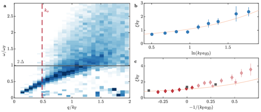
Supplementary Fig. S1: Pair size in the BEC-BCS crossover a: Estimation of the pair size from a measurement of the dynamic structure factor. We determine the onset momentum $k_{o}$ (red-dashed vertical line) of the pair breaking continuum via a bilinear fit of the dynamic structure factor $S(q,2\Delta)$ at a transferred energy of $\hbar\omega=2\Delta$ (black horizontal line). We then obtain an estimate of the pair size $\xi\approx\alpha_{3D}/k_{o}$. b: Estimate of the pair size $\xi=\alpha_{2D}/k_{o}$ for a 2D Fermi gas (blue circles). The value of $\alpha_{2D}\approx 0.6$ is obtained by matching our results for $k_{o}$ to the theoretical prediction Randeria et al. (1990) (solid line). c: Pair size $\xi=\alpha_{3D}/k_{o}$ for a 3D Fermi gas. Red stars denote data points where $k_{o}$ was extracted from full measurements of the 3D structure factor as shown in a, red diamonds denote data from a separate set of measurements where data was only taken at transferred energies of $\hbar\omega\approx 2\Delta$. The solid line denotes a theory prediction from ref. Marini et al. (1998), gray squares show results from a pair size measurement performed in ref. Schunck et al. (2008), rescaled as discussed in ref. Palestini and Strinati (2014). Error bars denote $1\sigma$ confidence intervals of the fit.

Material	$\nicefrac{{\Delta}}{{k_{B}}}$	$\nicefrac{{E_{\rm F}}}{{k_{B}}}$	$\xi$	$k_{\rm F}$	Ref.
	[K]	[K]	[Å]	[Å-1]
Bi2Sr2CaCu2O8	140	970	7.0	0.41	Harshman and Mills (1992); Yoshida et al. (2009)
Tl2Ba2Ca2Cu3O10	270	1800	7.3	0.49	Harshman and Mills (1992); Chia et al. (2011); Ponomarev et al. (2014)
La1.85Sr0.15CuO4	84	1100	11	0.46	Harshman and Mills (1992); Yoshida et al. (2009)
YBa2Cu3O7	470	8800	15	0.45	Harshman and Mills (1992); Grissonnanche et al. (2014); Dagan et al. (2000)
RbCa2Fe4As4F2	95	730	10	0.20	Adroja et al. (2018)
FeSe/STO	240	6200	6.7	0.61	Ge et al. (2015); Biswas et al. (2018)
Pb	13	120000	830	1.6	Carter et al. (1995)
Sn	6.6	110000	2300	1.6	Carter et al. (1995)
Al	2.1	110000	16000	1.6	Carter et al. (1995)
Nb	18	13000	111	0.54	Richards and Tinkham (1960); Townsend and Sutton (1962); Nakagawa et al. (2021)
BaKBiO3	61	2900	53	0.26	Escudero et al. (1994); Carter et al. (1995)
$\kappa$-(ET)2Cu(NCS)2	25	210	23	0.17	Harshman and Mills (1992); Wosnitza et al. (2003)
NbSe2	15	810	80	0.54	Le et al. (1991); Dvir et al. (2018)
PbMo6S8	36	1600	9.8	0.31	Harshman and Mills (1992); Petrović et al. (2011)
YB6	16	2400	330	0.41	Hillier and Cywinski (1997)
YNi2B2C	21	4200	80	0.94	Hillier and Cywinski (1997)
LuRuB2	16	4100	180	0.85	Lee et al. (1987); Barker et al. (2018a)
YRuB2	13	2400	110	0.84	Lee et al. (1987); Barker et al. (2018a)
K3C60	33	470	26	0.34	Uemura et al. (1991b); Degiorgi et al. (1994)
Rb3C60	62	2900	29	0.49	Degiorgi et al. (1994); Carter et al. (1995); Varshney et al. (2012)
Re3Ta	8.6	640	110	0.46	Barker et al. (2018b)
Re5.5Ta	16	2000	45	0.44	Singh et al. (2020)
Nb0.5Os0.5	5.6	660	78	0.15	Singh et al. (2018)
La7Ir3	4.3	520	190	0.40	Barker et al. (2015)
LaPtGe	4.9	1200	59	0.43	Sajilesh et al. (2018)
BeAu	5.8	18000	1900	1.1	Singh et al. (2019a)
TaOs	3.5	900	74	0.50	Singh et al. (2017)
Zr3Ir	4.1	1700	46	0.75	Singh et al. (2019b)
NbOs2	4.8	620	90	0.43	Singh et al. (2019c)
3He	0.0046	0.89	200	0.78	Movshovich et al. (1990); Pistolesi and Strinati (1994)
LixZrNCl	tuneable				Nakagawa et al. (2021)

Supplementary Table S1: Parameters for different fermionic superfluids in Fig. 4. Values and references for the superconducting gap $\Delta$, the Fermi energy $E_{\rm F}$, the coherence length $\xi$ and the Fermi wavevector $k_{\rm F}$ used in Fig. 4b. For materials such as cuprate superconductors where these parameters are dependent on the doping level, results for optimally doped samples were used. We note that there are different extrapolation methods and definitions of the coherence length, leading to different values between references. However, the differences are generally on the order of unity and therefore do not affect the conclusions drawn from Fig. 4b.

B [G]	$\ln(k_{\rm F}a_{\rm 2D})$	$\nicefrac{{\Delta}}{{E_{\rm F}}}$	$\nicefrac{{\mu}}{{E_{\rm F}}}$	$\xi k_{\rm F}$	B [G]	$(k_{\rm F}a_{\rm 3D})^{-1}$	$\nicefrac{{\Delta}}{{E_{\rm F}}}$	$\nicefrac{{\mu}}{{E_{\rm F}}}$	$\xi k_{\rm F}$
2D, Low $q$						3D, Low $q$
784	-0.55	1.084(4)	-0.83	-	812	0.37	0.64(7)	0.08	0.73
792	-0.29	0.98(1)	-0.53	-	816	0.27	0.573(7)	0.19	0.82
800	-0.07	0.87(1)	-0.31	-	820	0.22	0.58(1)	0.27	0.89
808	0.16	0.77(1)	-0.11	-	824	0.15	0.48(2)	0.32	1.01
816	0.33	0.71(1)	0.01	0.70	828	0.08	0.497(7)	0.38	1.18
824	0.50	0.64(1)	0.12	0.76	832	0.01	0.47(1)	0.44	1.41
855	1.10	0.47(2)	0.39	1.23	835	-0.05	0.44(2)	0.48	1.63
871	1.34	0.423(6)	0.46	1.52	839	-0.12	0.384(5)	0.53	1.93
886	1.58	0.410(5)	0.52	1.86	843	-0.18	0.38(1)	0.56	2.22
					847	-0.24	0.34(1)	0.59	2.54
2D, $S(\omega)$					855	-0.35	0.26(1)	0.64	3.16
824	0.50	0.61(1)	0.13	0.76
832	0.68	0.526(9)	0.22	0.85		3D, High $q$
839	0.82	0.55(1)	0.29	0.96	863	-0.43	0.222(3)	0.67	3.63
847	0.97	0.50(1)	0.35	1.09	867	-0.51	0.24(2)	0.69	4.04
855	1.11	0.493(9)	0.40	1.24	871	-0.53	0.193(7)	0.69	4.11
863	1.24	0.42(1)	0.44	1.40	879	-0.62	0.1686(5)	0.71	4.51
871	1.37	0.46(1)	0.47	1.56	886	-0.73	0.16(1)	0.73	-
886	1.61	0.383(5)	0.52	1.91	886	-0.74	0.14(2)	0.73	-
898	1.77	0.360(8)	0.55	2.17	894	-0.83	0.126(2)	0.74	-
910	1.92	0.31(1)	0.58	2.42	902	-0.91	0.11(1)	0.75	-
926	2.11	0.25(2)	0.61	2.75	910	-0.98	0.057(7)	0.76	-

Supplementary Table S2: Summary of experimental results. Shown are the measured values of the gap for both 2D and 3D Fermi gases, with the values for the 3D Fermi gases taken from Biss et al. (2021). Also shown are the values of the chemical potential $\mu$ used in Fig. 3 (see Supplementary Materials) and the approximate value of $\xi k_{\rm F}$ obtained from a spline fit to the data shown in Fig. 4a. Errors denote $1\sigma$ confidence intervals of the fit.

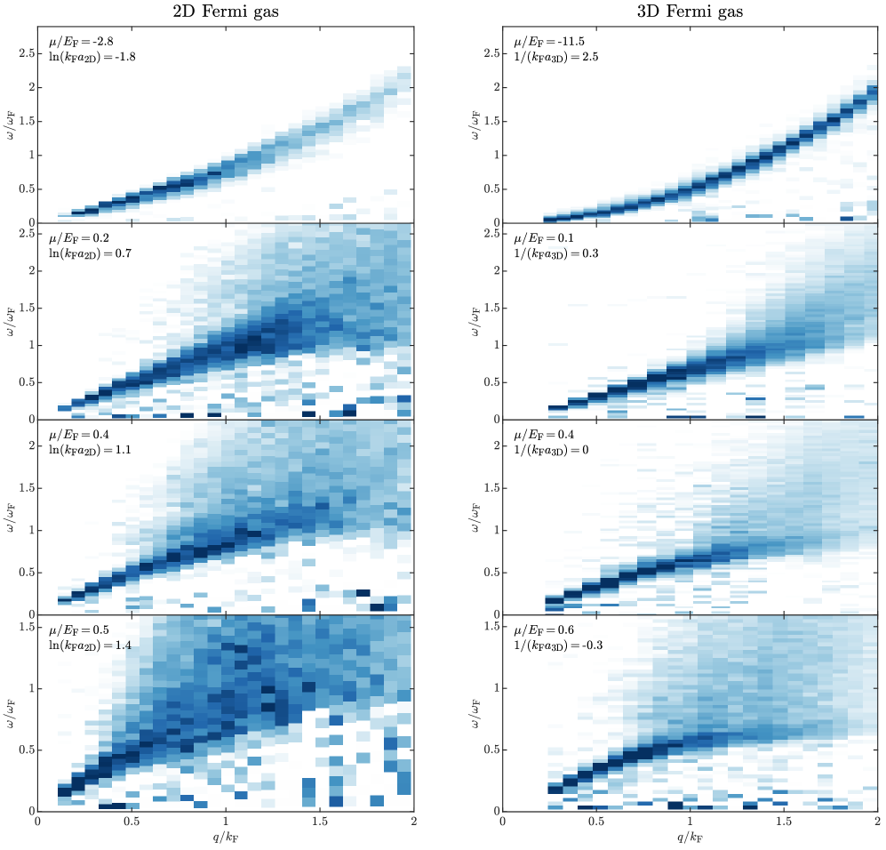
Supplementary Fig. S2: Measurements of the dynamic structure factor in two- and three-dimensional ultracold Fermi gases. The excitation spectra of systems with comparable values of $\mu/E_{\rm F}$ show very similar qualitative behavior. 3D data taken from Biss et al. (2021).

References

- Keimer et al. (2015) B. Keimer, S. A. Kivelson, M. R. Norman, S. Uchida, and J. Zaanen, Nature 518, 179 (2015).
- Ge et al. (2015) J.-F. Ge, Z.-L. Liu, C. Liu, C.-L. Gao, D. Qian, Q.-K. Xue, Y. Liu, and J.-F. Jia, Nat. Mater. 14, 285 (2015).
- Yu et al. (2019) Y. Yu, L. Ma, P. Cai, R. Zhong, C. Ye, J. Shen, G. D. Gu, X. H. Chen, and Y. Zhang, Nature 575, 156 (2019).
- Bloch et al. (2008) I. Bloch, J. Dalibard, and W. Zwerger, Rev. Mod. Phys. 80, 885 (2008).
- Ketterle and Zwierlein (2008) W. Ketterle and M. W. Zwierlein, in Proceedings of the International School of Physics-Enrico Fermi, edited by M Inguscio, S Stringari, (2008).
- Levinsen and Parish (2015) J. Levinsen and M. M. Parish, in Annual Review of Cold Atoms and Molecules, Annual Review of Cold Atoms and Molecules, Vol. 3 (WORLD SCIENTIFIC, 2015) pp. 1–75.
- Turlapov and Yu Kagan (2017) A. V. Turlapov and M. Yu Kagan, J. Phys. Condens. Matter 29, 383004 (2017).
- Biss et al. (2021) H. Biss, L. Sobirey, N. Luick, M. Bohlen, J. J. Kinnunen, G. M. Bruun, T. Lompe, and H. Moritz, (2021), arXiv:2105.09820 [cond-mat.quant-gas] .
- Bardeen et al. (1957) J. Bardeen, L. N. Cooper, and J. R. Schrieffer, Physical review 108, 1175 (1957).
- Uemura et al. (1991a) Y. J. Uemura, L. P. Le, G. M. Luke, B. J. Sternlieb, W. D. Wu, J. H. Brewer, T. M. Riseman, C. L. Seaman, M. B. Maple, M. Ishikawa, D. G. Hinks, J. D. Jorgensen, G. Saito, and H. Yamochi, Phys. Rev. Lett. 66, 2665 (1991a).
- Bohlen et al. (2020) M. Bohlen, L. Sobirey, N. Luick, H. Biss, T. Enss, T. Lompe, and H. Moritz, Phys. Rev. Lett. 124, 240403 (2020).
- Chin et al. (2010) C. Chin, R. Grimm, P. Julienne, and E. Tiesinga, Rev. Mod. Phys. 82, 1225 (2010).
- Martiyanov et al. (2010) K. Martiyanov, V. Makhalov, and A. Turlapov, Phys. Rev. Lett. 105, 030404 (2010).
- Fröhlich et al. (2011) B. Fröhlich, M. Feld, E. Vogt, M. Koschorreck, W. Zwerger, and M. Köhl, Phys. Rev. Lett. 106 (2011).
- Sommer et al. (2012) A. T. Sommer, L. W. Cheuk, M. J. H. Ku, W. S. Bakr, and M. W. Zwierlein, Phys. Rev. Lett. 108, 045302 (2012).
- Ries et al. (2015) M. G. Ries, A. N. Wenz, G. Zürn, L. Bayha, I. Boettcher, D. Kedar, P. A. Murthy, M. Neidig, T. Lompe, and S. Jochim, Phys. Rev. Lett. 114, 230401 (2015).
- Cheng et al. (2016) C. Cheng, J. Kangara, I. Arakelyan, and J. E. Thomas, Phys. Rev. A 94, 031606 (2016).
- Mitra et al. (2016) D. Mitra, P. T. Brown, P. Schauß, S. S. Kondov, and W. S. Bakr, Phys. Rev. Lett. 117, 093601 (2016).
- Peppler et al. (2018) T. Peppler, P. Dyke, M. Zamorano, I. Herrera, S. Hoinka, and C. J. Vale, Phys. Rev. Lett. 121, 120402 (2018).
- Hueck et al. (2018) K. Hueck, N. Luick, L. Sobirey, J. Siegl, T. Lompe, and H. Moritz, Phys. Rev. Lett. 120, 060402 (2018).
- Schirotzek et al. (2008) A. Schirotzek, Y.-I. Shin, C. H. Schunck, and W. Ketterle, Phys. Rev. Lett. 101, 140403 (2008).
- Hoinka et al. (2017) S. Hoinka, P. Dyke, M. G. Lingham, J. J. Kinnunen, G. M. Bruun, and C. J. Vale, Nat. Phys. 13, 943 (2017).
- Petrov and Shlyapnikov (2001) D. S. Petrov and G. V. Shlyapnikov, Phys. Rev. A 64, 012706 (2001).
- Note (1) While in principle a third type of excitations exists in the form of the Higgs mode, this mode is expected to lie within the pair breaking continuum Zhao et al. (2020)) and is therefore not visible in our spectra.
- Goldstone (1961) J. Goldstone, Il Nuovo Cimento (1955-1965) 19, 154 (1961).
- Leggett (1998) A. J. Leggett, J. Phys. Chem. Solids 59, 1729 (1998).
- Büchler et al. (2004) H. P. Büchler, P. Zoller, and W. Zwerger, Phys. Rev. Lett. 93, 080401 (2004).
- Randeria et al. (1989) M. Randeria, J. M. Duan, and L. Y. Shieh, Phys. Rev. Lett. 62, 981 (1989).
- Vitali et al. (2017) E. Vitali, H. Shi, M. Qin, and S. Zhang, Phys. Rev. A 96, 061601 (2017).
- Zielinski et al. (2020) T. Zielinski, B. Ross, and A. Gezerlis, Phys. Rev. A 101, 033601 (2020).
- Devereaux and Hackl (2007) T. P. Devereaux and R. Hackl, Rev. Mod. Phys. 79, 175 (2007).
- Klein and Dierker (1984) M. V. Klein and S. B. Dierker, Phys. Rev. B Condens. Matter 29, 4976 (1984).
- Astrakharchik et al. (2004) G. E. Astrakharchik, J. Boronat, J. Casulleras, Giorgini, and S, Phys. Rev. Lett. 93, 200404 (2004).
- Shi et al. (2015) H. Shi, S. Chiesa, and S. Zhang, Phys. Rev. A 92, 033603 (2015).
- Haussmann et al. (2007) R. Haussmann, W. Rantner, S. Cerrito, and W. Zwerger, Phys. Rev. A 75, 023610 (2007).
- (36) Note that we plot the gap from Haussmann et al. (2007) against the chemical potential from Astrakharchik et al. (2004) instead of the value for obtained in Haussmann et al. (2007). However, as the two results for the chemical potential are very similar, this does not significantly affect the comparison or its conclusion.
- Ashcroft and Mermin (1976) N. W. Ashcroft and N. D. Mermin, Solid state physics (New York: Holt, Rinehart and Winston,, 1976).
- Boettcher et al. (2016) I. Boettcher, L. Bayha, D. Kedar, P. A. Murthy, M. Neidig, M. G. Ries, A. N. Wenz, G. Zürn, S. Jochim, and T. Enss, Phys. Rev. Lett. 116, 045303 (2016).
- Ku et al. (2012) M. J. H. Ku, A. T. Sommer, L. W. Cheuk, and M. W. Zwierlein, Science 335, 563 (2012).
- Pistolesi and Strinati (1994) F. Pistolesi and G. C. Strinati, Phys. Rev. B Condens. Matter 49, 6356 (1994).
- Stintzing and Zwerger (1997) S. Stintzing and W. Zwerger, Phys. Rev. B Condens. Matter 56, 9004 (1997).
- Schunck et al. (2008) C. H. Schunck, Y.-I. Shin, A. Schirotzek, and W. Ketterle, Nature 454, 739 (2008).
- Marsiglio et al. (2015) F. Marsiglio, P. Pieri, A. Perali, F. Palestini, and G. C. Strinati, Phys. Rev. B Condens. Matter 91, 054509 (2015).
- Pistolesi and Strinati (1996) F. Pistolesi and G. C. Strinati, Phys. Rev. B Condens. Matter 53, 15168 (1996).
- Randeria et al. (1990) M. Randeria, J. M. Duan, and L. Y. Shieh, Phys. Rev. B Condens. Matter 41, 327 (1990).
- Marini et al. (1998) M. Marini, F. Pistolesi, and G. C. Strinati, Eur. Phys. J. B 1, 151 (1998).
- Park et al. (2021) J. M. Park, Y. Cao, K. Watanabe, T. Taniguchi, and P. Jarillo-Herrero, Nature 590, 249 (2021).
- Nakagawa et al. (2021) Y. Nakagawa, Y. Kasahara, T. Nomoto, R. Arita, T. Nojima, and Y. Iwasa, Science 372, 190 (2021).
- Murthy et al. (2018) P. A. Murthy, M. Neidig, R. Klemt, L. Bayha, I. Boettcher, T. Enss, M. Holten, G. Zürn, P. M. Preiss, and S. Jochim, Science 359, 452 (2018).
- Kondo et al. (2011) T. Kondo, Y. Hamaya, A. D. Palczewski, T. Takeuchi, J. S. Wen, Z. J. Xu, G. Gu, J. Schmalian, and A. Kaminski, Nat. Phys. 7, 21 (2011).
- Kondo et al. (2013) T. Kondo, A. D. Palczewski, Y. Hamaya, T. Takeuchi, J. S. Wen, Z. J. Xu, G. Gu, and A. Kaminski, Phys. Rev. Lett. 111, 157003 (2013).
- Hashimoto et al. (2014) M. Hashimoto, I. M. Vishik, R.-H. He, T. P. Devereaux, and Z.-X. Shen, Nat. Phys. 10, 483 (2014).
- Zhao et al. (2020) H. Zhao, X. Gao, W. Liang, P. Zou, and F. Yuan, New J. Phys. 22, 093012 (2020).

References

- (1)
- Sobirey et al. (2021) L. Sobirey, N. Luick, M. Bohlen, H. Biss, H. Moritz, and T. Lompe, Science 372, 844 (2021).
- Zürn et al. (2013) G. Zürn, T. Lompe, A. N. Wenz, S. Jochim, P. S. Julienne, and J. M. Hutson, Phys. Rev. Lett. 110 (2013).
- Brunello et al. (2001) A. Brunello, F. Dalfovo, L. Pitaevskii, S. Stringari, and F. Zambelli, Phys. Rev. A 64, 063614 (2001).
- Kuhnle et al. (2011) E. D. Kuhnle, S. Hoinka, P. Dyke, H. Hu, P. Hannaford, and C. J. Vale, Phys. Rev. Lett. 106, 170402 (2011).
- Navon et al. (2010) N. Navon, S. Nascimbène, F. Chevy, and C. Salomon, Science 328, 729 (2010).
- Fenech et al. (2016) K. Fenech, P. Dyke, T. Peppler, M. G. Lingham, S. Hoinka, H. Hu, and C. J. Vale, Phys. Rev. Lett. 116, 045302 (2016).
- Palestini and Strinati (2014) F. Palestini and G. C. Strinati, Phys. Rev. B Condens. Matter 89, 224508 (2014).
- Harshman and Mills (1992) D. R. Harshman and A. P. Mills, Phys. Rev. B Condens. Matter 45, 10684 (1992).
- Yoshida et al. (2009) T. Yoshida, M. Hashimoto, S. Ideta, A. Fujimori, K. Tanaka, N. Mannella, Z. Hussain, Z.-X. Shen, M. Kubota, K. Ono, and Others, Phys. Rev. Lett. 103, 037004 (2009).
- Chia et al. (2011) E. E. M. Chia, J.-X. Zhu, D. Talbayev, and A. J. Taylor, Phys. Stat. Solidi. Rapid Res. Lett. 5, 1 (2011).
- Ponomarev et al. (2014) Y. G. Ponomarev, V. A. Alyoshin, E. V. Antipov, T. E. Oskina, A. Krapf, S. V. Kulbachinskii, M. G. Mikheev, M. V. Sudakova, S. N. Tchesnokov, and L. M. Fisher, JETP Lett. 100, 126 (2014).
- Grissonnanche et al. (2014) G. Grissonnanche, O. Cyr-Choinière, F. Laliberté, S. René de Cotret, A. Juneau-Fecteau, S. Dufour-Beauséjour, M.-È. Delage, D. LeBoeuf, J. Chang, B. J. Ramshaw, D. A. Bonn, W. N. Hardy, R. Liang, S. Adachi, N. E. Hussey, B. Vignolle, C. Proust, M. Sutherland, S. Krämer, J.-H. Park, D. Graf, N. Doiron-Leyraud, and L. Taillefer, Nat. Commun. 5, 3280 (2014).
- Dagan et al. (2000) Y. Dagan, R. Krupke, and G. Deutscher, Phys. Rev. B: Condens. Matter Mater. Phys. 62, 146 (2000).
- Adroja et al. (2018) D. T. Adroja, F. K. K. Kirschner, F. Lang, M. Smidman, A. D. Hillier, Z.-C. Wang, G.-H. Cao, G. B. G. Stenning, and S. J. Blundell, J. Phys. Soc. Jpn. 87, 124705 (2018).
- Biswas et al. (2018) P. K. Biswas, Z. Salman, Q. Song, R. Peng, J. Zhang, L. Shu, D. L. Feng, T. Prokscha, and E. Morenzoni, Phys. Rev. B Condens. Matter 97, 174509 (2018).
- Carter et al. (1995) R. M. Carter, M. Casas, J. M. Getino, M. de Llano, A. Puente, H. Rubio, and D. van der Walt, Phys. Rev. B Condens. Matter 52, 16149 (1995).
- Richards and Tinkham (1960) P. L. Richards and M. Tinkham, Phys. Rev. 119, 575 (1960).
- Townsend and Sutton (1962) P. Townsend and J. Sutton, Phys. Rev. 128, 591 (1962).
- Escudero et al. (1994) R. Escudero, E. Verdin, and F. Morales, J. Supercond. 7, 381 (1994).
- Wosnitza et al. (2003) J. Wosnitza, S. Wanka, J. Hagel, M. Reibelt, D. Schweitzer, and J. A. Schlueter, Synth. Met. 133-134, 201 (2003).
- Le et al. (1991) L. P. Le, G. M. Luke, B. J. Sternlieb, W. D. Wu, Y. J. Uemura, J. W. Brill, and H. Drulis, Physica C Supercond. 185-189, 2715 (1991).
- Dvir et al. (2018) T. Dvir, F. Massee, L. Attias, M. Khodas, M. Aprili, C. H. L. Quay, and H. Steinberg, Nat. Commun. 9, 1 (2018).
- Petrović et al. (2011) A. P. Petrović, R. Lortz, G. Santi, C. Berthod, C. Dubois, M. Decroux, A. Demuer, A. B. Antunes, A. Paré, D. Salloum, and Others, Phys. Rev. Lett. 106, 017003 (2011).
- Hillier and Cywinski (1997) A. D. Hillier and R. Cywinski, Appl. Magn. Reson. 13, 95 (1997).
- Lee et al. (1987) W. H. Lee, S. Appl, and R. N. Shelton, J. Low Temp. Phys. 68, 147 (1987).
- Barker et al. (2018a) J. A. T. Barker, R. P. Singh, A. D. Hillier, and D. M. Paul, Phys. Rev. B Condens. Matter 97, 094506 (2018a).
- Uemura et al. (1991b) Y. J. Uemura, A. Keren, L. P. Le, G. M. Luke, B. J. Sternlieb, W. D. Wu, J. H. Brewer, R. L. Whetten, S. M. Huang, S. Lin, R. B. Kaner, F. Diederich, S. Donovan, G. Grüner, and K. Holczer, Nature 352, 605 (1991b).
- Degiorgi et al. (1994) L. Degiorgi, G. Briceno, M. S. Fuhrer, A. Zettl, and P. Wachter, Nature 369, 541 (1994).
- Varshney et al. (2012) D. Varshney, R. Jain, and N. Singh, Journal of Theoretical and Applied Physics 6, 25 (2012).
- Barker et al. (2018b) J. A. T. Barker, B. D. Breen, R. Hanson, A. D. Hillier, M. R. Lees, G. Balakrishnan, D. M. Paul, and R. P. Singh, Phys. Rev. B: Condens. Matter Mater. Phys. 98, 104506 (2018b).
- Singh et al. (2020) D. Singh, P. K. Biswas, A. D. Hillier, R. P. Singh, and Others, Phys. Rev. B: Condens. Matter Mater. Phys. 101, 144508 (2020).
- Singh et al. (2018) D. Singh, J. A. T. Barker, A. Thamizhavel, A. D. Hillier, D. M. Paul, and R. P. Singh, J. Phys. Condens. Matter 30, 075601 (2018).
- Barker et al. (2015) J. A. T. Barker, D. Singh, A. Thamizhavel, A. D. Hillier, M. R. Lees, G. Balakrishnan, D. M. Paul, and R. P. Singh, Phys. Rev. Lett. 115, 267001 (2015).
- Sajilesh et al. (2018) K. P. Sajilesh, D. Singh, P. K. Biswas, A. D. Hillier, and R. P. Singh, Phys. Rev. B Condens. Matter 98, 214505 (2018).
- Singh et al. (2019a) D. Singh, A. D. Hillier, and R. P. Singh, Phys. Rev. B Condens. Matter 99, 134509 (2019a).
- Singh et al. (2017) D. Singh, K. P. Sajilesh, S. Marik, A. D. Hillier, and R. P. Singh, Supercond. Sci. Technol. 30, 125003 (2017).
- Singh et al. (2019b) D. Singh, P. K. Biswas, G. B. G. Stenning, A. D. Hillier, R. P. Singh, and Others, Physical Review Materials 3, 104802 (2019b).
- Singh et al. (2019c) D. Singh, S. K. P., S. Marik, A. D. Hillier, and R. P. Singh, Phys. Rev. B Condens. Matter 99, 014516 (2019c).
- Movshovich et al. (1990) R. Movshovich, N. Kim, and D. M. Lee, Phys. Rev. Lett. 64, 431 (1990).