Failing with Grace: Learning Neural Network Controllers that are Boundedly Unsafe

Abstract

In this work, we consider the problem of learning a feed-forward neural network controller to safely steer an arbitrarily shaped planar robot in a compact and obstacle-occluded workspace. Unlike existing methods that depend strongly on the density of data points close to the boundary of the safe state space to train neural network controllers with closed-loop safety guarantees, here we propose an alternative approach that lifts such strong assumptions on the data that are hard to satisfy in practice and instead allows for graceful safety violations, i.e., of a bounded magnitude that can be spatially controlled. To do so, we employ reachability analysis techniques to encapsulate safety constraints in the training process. Specifically, to obtain a computationally efficient over-approximation of the forward reachable set of the closed-loop system, we partition the robot’s state space into cells and adaptively subdivide the cells that contain states which may escape the safe set under the trained control law. Then, using the overlap between each cell’s forward reachable set and the set of infeasible robot configurations as a measure for safety violations, we introduce appropriate terms into the loss function that penalize this overlap in the training process. As a result, our method can learn a safe vector field for the closed-loop system and, at the same time, provide worst-case bounds on safety violation over the whole configuration space, defined by the overlap between the over-approximation of the forward reachable set of the closed-loop system and the set of unsafe states. Moreover, it can control the tradeoff between computational complexity and tightness of these bounds. Our proposed method is supported by both theoretical results and simulation studies.

I Introduction

In recent years, progress in the field of machine learning has furnished a new family of neural network controllers for robotic systems that have significantly simplified the overall design process. Robot navigation is one application where neural network controllers have been successfully employed for steering a variety of robots in static and dynamic environments [1, 2, 3, 4, 5]. As such control schemes become more common in real-world applications, the ability to train neural networks with safety considerations becomes a necessity.

The design of reliable data-driven controllers that result in safe and adaptable closed-loop systems has typically relied on methods that couple state-of-the-art machine learning algorithms with control [6, 7]. A popular approach that falls in this class of methods employs control barrier functions to appropriately constrain the control inputs computed using data-driven techniques so that a specified safe subset of the state space remains invariant during execution and learning. For example, [8] employs control barrier functions to safeguard the exploration and deployment of a reinforcement learning policy trained to achieve high-level temporal specifications. Similarly, [9] pairs adaptive model learning with barrier certificates for systems with possibly non-stationary agent dynamics. Safety during learning is accomplished in [10] by combining model-free reinforcement learning with barrier certificates and using Gaussian Processes to model the systems dynamics. Although barrier certificates constitute an intuitive tool for ensuring safety constraints, designing appropriate barrier functions for robotic systems operating in complex environments is generally a hard problem. As a result, simple but rather conservative certificates are typically used in practice. Additionally, conflicts between the reference control laws and the barrier certificates may introduce unwanted equilibria to the closed-loop system. A method to address this problem is proposed in [11, 12] that learns control barrier functions from expert demonstrations. However, this method requires dense enough sampled data as well as the Liptchitz constants of the system’s dynamics and corresponding neural network controller that are hard to obtain in practice.

Compared to the control barrier function methods discussed above that can usually only ensure invariance of a conservative subset of the set of safe states, backwards reachability methods can instead compute the exact set of safe states which, similar to control barrier function methods, can then be rendered invariant by an appropriate design of controllers that take over when the system approaches the boundary of that safe set. However, exact computation of the safe set using backwards reachability methods generally comes at the expense of higher computational cost. Such a method is presented in [13] that employs Hamilton-Jacobi reachability to compute the set of safe states for which control inputs exist that prevent the system from violating safety specifications. Then, a supervisory control policy is proposed that feeds the output of a nominal neural network controller to the system when the state lies inside the safe set and switches to a fail-safe optimal control law that can drive the system’s state back to the safe set, when the nominal controller drives the system outside the safe set. This supervisory control law is extended in [14] to address model uncertainty by learning bounds on the unknown disturbances online and utilizing them to derive probabilistic guarantees on safety. In [15], Hamilton-Jacobi reachability is also used to generate safe and optimal trajectories that are used as data to train convolutional neural networks that yield waypoints which can be tracked robustly by the robot equipped with a conventional feedback controller.

Common in the methods discussed above is that they generally apply reachability analysis on the open loop dynamics without considering the specific structure of the reference neural network controller, owning to its complexity. Reachability analysis of neural networks is an actively studied topic and recent solutions have been proposed for verification [16, 17, 18] and robust training [19, 20] alike. These methods have been successfully adapted for estimating the forward reachable set of dynamical systems in feedback interconnection with feed-forward neural network controllers. For example, in [21, 22], Taylor models are used to compute an over-approximation of the closed-loop system’s reachable set by constructing a polynomial approximation of the neural network controller. An alternative approach to this problem is proposed in [23] that translates activation functions into quadratic constraints and formulates a semi-definite program in order to compute an over-approximation of forward reachable sets of the closed-loop system. Over-approximations of the forward reachable set can also be computed using interval subdivision methods as shown in [24]. In this work, the robot’s state space is partitioned into smaller cells with specified size and the controller’s output set is approximated by the union of each cell’s output reachable set over-approximation. To reduce the fineness of the partition and, effectively, minimize computational cost, heuristic methods have been developed in [25, 26]. Although the methods discussed above provide accurate over-approximations of the reachable set of neural network controllers, they only address the verification problem of already trained controllers and do not consider safety specifications.

In this work, we consider the problem of training a neural network controller in feedback interconnection with a polygonal shaped robot, able to translate and rotate within a compact, obstacle-occluded workspace, such that the closed-loop system safely reaches a specified goal configuration and possible safety violations are explicitly bounded. Specifically, given a dataset of state and input pairs sampled from safe robot trajectories, we first train a feed-forward neural network controller so that the closed-loop system fits the vector field implicitly defined by the data. Then, we propose a new supervised learning method to iteratively re-train the neural network controller so that safety specifications are satisfied, namely, the robot is steered away from states that can result in collisions with the obstacles. To do so, at each re-training iteration, we compute an over-approximation of the robot’s forward reachable set under the current trained controller using the Interval Bound Propagation (IBP) method [24] and update the loss function with appropriate penalty terms used to minimize the overlap between this over-approximation of the forward reachable set and the set of unsafe states. Since the robot configuration space and, therefore, the safe set of states needed to compute the robot’s forward reachable set, are difficult to obtain explicitly due to the arbitrary geometry of the robot and the workspace, we use the adaptive partitioning method proposed in [27] to obtain a simpler over-approximation of this safe set. Particularly, we construct a cover of the set of feasible robot states consisting of rectangular cells that either contain only safe configurations or intersect with the boundary of the safe set and, thus, contain both safe and unsafe states. Then, we compute suitable under- and over-approximations of the robot’s footprint which we use to determine whether a given cell contains only safe states or not. Cells that lie on the boundary of the safe set and, therefore, contain unsafe states, are recursively subdivided until a tight enough cover is obtained. Since the quality of the over-approximation of the forward reachable set depends on the accuracy of the over-approximation of the safe set and on the parameters of the neural network controller, which are updated with every re-training iteration, we also propose a method to refine the cell partition of the safe set at each iteration by subdividing and/or merging cells based on the overlap between the over-approximation of their forward reachable sets and the set of unsafe states. This way, we can control the tradeoff between computational complexity and tightness of the safety violation bounds. Finally, we provide a simulation study that verifies the efficacy of the proposed scheme.

To the best of our knowledge, this is the first safe learning framework for neural network controllers that (i) provides numerical worst-case bounds on safety violation over the whole configuration space, defined by the overlap between the over-approximation of the forward reachable set of the closed-loop system and the set of unsafe states, and (ii) controls the tradeoff between computational complexity and tightness of these bounds. Compared to the methods in [10, 11, 13] that employ control barrier functions or Hamilton-Jacobi reachability to design fail-safe projection operators or supervisory control policies, respectively, that can be wrapped around pre-trained nominal neural network controllers that are possibly unsafe due to, e.g., insufficient data during training, here we directly train neural network controllers with safety specifications in mind. On the other hand, unlike the methods in [15, 9, 10] that also directly train safe neural network controllers using sufficiently many safe-by-design training samples, here safety of the closed-loop system does not depend on data points, but on safety violation bounds defined over the whole configuration space that enter explicitly the loss function as penalty terms during training. As a result, when our method fails to guarantee safety of the closed-loop system in the whole configuration space, it does so with grace by also providing safety violation bounds whose size can be controlled. Such guarantees on the closed-loop performance cannot be obtained using the methods in [15, 9, 10] that critically depend on the density of sampling. While the heuristic methods in [25, 26] can obtain tight bounds on the controller outputs used to verify the robustness of the controlled system, they do so by considering the reachable set of the controller instead of the closed-loop dynamics. The key idea in this work that allows us to control tightness of the safety violation bounds as a function of the computational cost is that the partition of the safe set into cells is guided by the overlap between the over-approximation of the forward reachable set of the closed-loop system and the set of unsafe states, which itself measures safety violation. Therefore, cells located far from the boundary of the safe set are not unnecessarily subdivided given that they do not require precise control input bounds to be labeled as safe. As a result, the partition of the safe set computed by our method consists of noticeably fewer cells compared to the number of cells returned by brute-force subdividing the safe set to achieve the same tightness of safety violation bounds. The effect of a smaller partition is fewer reachable set evaluations required at each iteration of the training process; a unique feature of the proposed method. Our approach is inspired by the methods proposed in [20, 19] that use reachability analysis to train robust neural networks for regression and classification. Here, we extend these subdivision-based reachability analysis algorithms to learn safe neural network controllers.

Perhaps most closely related to the method proposed here is the approach in [28] that also trains provably safe neural network controllers for robot navigation. Specifically, given an arbitrary fixed partition of the robot’s state space and the controller’s parameter space, [28] employs reachability analysis to build a transition graph and identify regions of control parameters (i.e., weights and biases) for which the closed-loop system is guaranteed to be safe. Then, a distinct ReLU neural network controller is trained for every state space cell using standard learning methods augmented by a projection operator that restricts the trained neural network weights to the regions found to be safe. Compared to [28], the method proposed here is not restricted to ReLU neural networks and can accommodate any class of strictly increasing continuous activation functions. Moreover, the method proposed here applies to non-point robots and returns smooth trajectories that respect the robot dynamics. To the contrary, [28] applies to point robots and returns trajectories that are non-smooth due to possible discontinuities when the ReLU neural network controllers are stitched together at consecutive state space cells. Finally, feasibility of the control synthesis problem in [28] strongly relies on the availability of sufficient data needed to train neural network weights that belong to the regions found to be safe. Instead, the method proposed here removes such strong assumptions on data that are hard to satisfy in practice and instead allows for graceful safety violations, of a bounded magnitude that can be spatially controlled.

We organize the paper as follows. In Section II, we formulate the problem under consideration while in Section III we develop the proposed adaptive subdivision method that relies on reachability analysis techniques to partition the safe set into cells and present the proposed safety-aware learning method. Finally, in Section IV we conclude this work by presenting results corroborating the efficacy of our scheme.

Notation: We will refer to an interval of the set of real numbers $\mathbb{R}$ as a simple interval, whereas the Cartesian product of one or more simple intervals will be referred to as a composite interval. An $n$-dimensional interval is a composite interval of the form $[x_{l,1},x_{u,1}]\times[x_{l,2},x_{u,2}]\times\ldots\times[x_{l,n},x_{u,n}]$. Given a compact set $\mathcal{S}\in\mathbb{R}^{n}$ and a vector $\delta=[\delta_{1},\delta_{2},\ldots,\delta_{n}]\in\mathbb{R}^{n}$ we shall use $\mathrm{vol}_{\delta}\left({\mathcal{S}}\right)$ to denote the volume of $\mathcal{S}$ after scaling the $i$-th dimension by the $\delta_{i}$, i.e., $\mathrm{vol}_{\delta}\left({\mathcal{S}}\right)=\prod_{i=1}^{n}{\delta_{i}\cdot(x_{u,i}-x_{l,i})}$. For brevity, we shall write $\mathrm{vol}\left({\mathcal{S}}\right)$ to denote $\mathrm{vol}_{\delta}\left({\mathcal{S}}\right)$ when $\delta=[1,1,\ldots,1]$. Given a set, $\mathcal{S}$, $\mathfrak{S}(\mathcal{S})$ is the set of all its compact subsets. We will denote $\mathcal{C}_{r}=[-r,r]^{3}$ and $\mathcal{B}_{r}=\{x\in\mathbb{R}|||x||\leq r\}$ The zero element in any vector space will be denoted $\mathrm{0}$.

II Problem Formulation

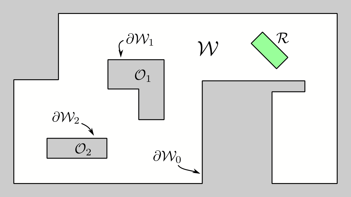
Figure 1: Robot $\mathcal{R}$ operating within a workspace $\mathcal{W}$ occupied by two inner obstacles.

We consider a polygonal shaped robot $\mathcal{R}$ operating within a compact, static workspace $\mathcal{W}\subset\mathbb{R}^{2}$ defined by an outer boundary $\partial\mathcal{W}_{0}$ and $N_{\mathcal{O}}$ inner boundaries $\partial\mathcal{W}_{i},i\in\mathfrak{I}_{\mathcal{O}}\triangleq\left\{{1,2,\ldots,N_{\mathcal{O}}}\right\}$, corresponding to a set of disjoint, fixed inner obstacles $\mathcal{O}_{i}$, as seen in Figure 1. We assume that the boundary $\partial\mathcal{R}$ of the robot’s body and the boundaries $\partial\mathcal{W}_{0},\partial\mathcal{W}_{i},i\in\mathfrak{I}_{\mathcal{O}}$ of the workspace are polygonal Jordan curves. Let $\mathcal{F}_{\mathcal{W}}$ and $\mathcal{F}_{\mathcal{R}}$ be coordinate frames arbitrarily embedded in the workspace and on the robot, respectively, and let $p=\left[{x,y,\theta}\right]^{T}$ denote the configuration of the robot on the plane, specifying the relative position $\left[{x,y}\right]^{T}\in\mathbb{R}^{2}$ and the orientation $\hat{n}\left({\theta}\right)={[\cos{\theta},\sin{\theta}]}^{T}$, $\theta\in[0,2\pi)$, of $\mathcal{F}_{\mathcal{R}}$ with respect to $\mathcal{F}_{\mathcal{W}}$. We assume that the robot is able to translate and rotate subject to the following discrete-time non-linear dynamics

$$z_{k+1}=f\left({{z_{k}},{u_{k}}}\right),$$ (1)

where $z=\left[{p^{T},q^{T}}\right]^{T}\in\mathcal{Z}\subset\mathbb{R}^{n}$, and $u\in\mathbb{R}^{m}$ denote the robot’s state and control input, respectively, and $q$ denotes miscellaneous robot states, e.g., linear and angular velocities, accelerations, etc. We define $\mathcal{Z}\triangleq\mathcal{Z}_{[p]}\times\mathcal{Z}_{[q]}$, where $\mathcal{Z}_{[p]}=\mathcal{W}\times\mathbb{S}^{1}$, and $\mathcal{Z}_{[q]}\subset\mathbb{R}^{n-3}$ is a $(n-3)$-dimensional interval of miscellaneous safe robot states, e.g., allowed bounds on the robot’s velocities. The non-linear function $f:\mathbb{R}^{n}\mapsto\mathbb{R}^{n}$ is assumed known and continuously differentiable. Furthermore, we assume that a function $F$ is known which maps composite intervals $\mathcal{A}$ and $\mathcal{B}$ of $\mathcal{Z}$ and $\mathbb{R}^{m}$, respectively, to composite intervals of $\mathcal{Z}$ such that

$$f\left({{z},{u}}\right)\in F\left({{\mathcal{A}},{\mathcal{B}}}\right),~{}~{}~{}\forall z,u\in\mathcal{A}\times\mathcal{B}.$$ (2)

In order to steer the robot to a desired feasible state $z^{\star}$, we equip the robot with a feed-forward multi-layer neural network controller $\phi:\mathbb{R}^{n}\mapsto\mathbb{R}^{m}$ that consists of $N_{\phi}$ fully connected layers, i.e.,

$$u=\phi(z)=\phi_{N_{\phi}}{\left(\phi_{N_{\phi}-1}{\left(\ldots\phi_{1}{\left(z\right)}\ldots\right)}\right)},$$ (3)

$$\phi_{i}{\left(x\right)}=h_{i}{\left({w_{i}\cdot x+b_{i}}\right)},~{}~{}~{}\forall i\in\mathfrak{I}_{N_{\phi}},$$ (4)

where $w_{i},b_{i},h_{i}$ denote the weight matrix, bias vector and activation function of the $i$-th layer, for all $i\in\mathfrak{I}_{N_{\phi}}$. Specifically, the $i$-th layer of $\phi$ consists of $n_{i}$ neurons, i.e., $w_{i}\in\mathbb{R}^{n_{i}\times n_{i-1}}$, $b_{i}\in\mathbb{R}^{n_{i}\times 1}$, $h_{i}\in\mathbb{R}^{n_{i}\times 1}$, for all $i\in\mathfrak{I}_{N_{\phi}}$ where $n_{0}=n$ and $n_{N_{\phi}}=m$.

To find values for $w_{i},b_{i},i\in\mathfrak{I}_{N_{\phi}}$ such that the controller $\phi$ can steer the robot to the desired state $z^{\star}$, we assume that we are given a set $\mathcal{D}$ consisting of points $(z_{i},u_{i})\in\mathcal{Z}\times\mathbb{R}^{m}$ sampled from robot trajectories beginning at different random states $z\in\mathcal{Z}$ and terminating at $z^{\star}$. Additionally, we assume that the given trajectories are feasible in the sense that they consist entirely of states that are safe. A state $z=\left[{p^{T},q^{T}}\right]^{T}$ is said to be safe if $q\in\mathcal{Z}_{[q]}$ and the robot at the corresponding configuration does not overlap with any of the static obstacles, i.e., $\mathcal{R}\left({p}\right)\subset\mathcal{W}$ where $\mathcal{R}\left({p}\right)$, denotes the robot’s footprint when it is placed at $\left[{x,y}\right]^{T}$ with orientation $\theta$. If the parameter space of the network $\phi$ and the dataset $\mathcal{D}$ are large enough, parameters $w,b$ can be typically found by solving the optimization problem

$$\begin{aligned} &\underset{w,b}{\text{minimize}}&&J\left({w,b}\right)\\ \end{aligned},$$ (5)

where

$$J\left({w,b}\right)=\lambda_{B}\cdot\sum_{\left({z,u}\right)\in\mathcal{D}}{\left({u-\phi\left({z;w,b}\right)}\right)^{2}}+\lambda_{R}\cdot r\left({w,b}\right).$$ (6)

In the loss function (6), $w=\left[{w_{1},w_{2},\ldots,w_{N_{\phi}}}\right]$ , $b=\left[{b_{1},b_{2},\ldots,b_{N_{\phi}}}\right]$ , $r\left({\cdot}\right)$ is a regularization term and $\lambda_{B}$, $\lambda_{R}$ are positive constants. We remark that the controller obtained from the solution of the problem (5)-(6) is expected to be safe only around the trajectories in the training dataset $\mathcal{D}$. This behavior is generally not desirable. Instead, what is desired is that the robot dynamics (1) under the control law (3) ensure that the safe set of states $\mathcal{Z}_{s}$ remains invariant, where $\mathcal{Z}_{s}$ consists of all the states $\left({p,q}\right)\in\mathcal{Z}$ such that $\mathcal{R}\left({p}\right)\subset\mathcal{W}$. Therefore, in this paper we consider the following problem.

Problem 1.

Given a static workspace $\mathcal{W}$, a polygonal robot $\mathcal{R}$ subject to dynamics $f$, a safe set of miscellaneous robot states $\mathcal{Z}_{[q]}$, and a dataset $\mathcal{D}$, train a neural network controller $\phi$ so that the closed-loop trajectories fit the data in the set $\mathcal{D}$ and the safe set $\mathcal{Z}_{s}$ either remains invariant or possible safety violations are explicitly bounded.

III Methodology

In order to address Problem 1, we first employ standard learning methods to solve the optimization problem (5) and obtain initial values for the parameters $w$ and $b$. As discussed before, the controller $\phi$ obtained at this stage is expected to be safe only around the points in $\mathcal{D}$, assuming that they have been sampled from safe trajectories and the network fits the dataset adequately. Next, we employ the subdivision method presented in subsection III-A to obtain a partition $\mathcal{P}$ of the feasible space into cells that provide a tight over-approximation $\overline{\mathcal{Z}}_{s}$ of the robot’s safe state space $\mathcal{Z}_{s}$. Using the over-approximation of the safe set $\mathcal{Z}_{s}$ as a set of initial robot states, in subsection III-B, we compute an over-approximation $\overline{\mathcal{Z}}_{c}$ of the forward reachable set $\mathcal{Z}_{c}$ of the closed loop system under the neural network controller $\phi$. Since the accuracy of the over-approximation $\overline{\mathcal{Z}}_{c}$ depends on the partition $\mathcal{P}$ of the over-approximation of the safe set $\overline{\mathcal{Z}}_{s}$, we also propose a method to refine the partition in order to improve the accuracy of the over-approximation $\overline{\mathcal{Z}}_{c}$. Finally, in subsection III-C, we use the overlap between the over-approximation of the forward reachable set $\overline{\mathcal{Z}}_{c}$ and the set of unsafe states to design penalty terms in problem (5) that explicitly capture safety specifications. As the parameters $w,b$ of the neural network $\phi$ get updated, so does the shape of the forward reachable set $\overline{\mathcal{Z}}_{c}$, which implies that the initial partition $\mathcal{P}$ of the over-approximation of the safe set $\overline{\mathcal{Z}}_{s}$ does no longer accurately approximate $\mathcal{Z}_{c}$. For this reason, we repeat the partition refinement and training steps proposed in subsection III-B and subsection III-C for a sufficiently large number of epochs $N_{\mathrm{epochs}}$. The procedure described above is outlined in Algorithm 1.

1function $\{w,\ b\}=$Train($\epsilon_{w},\ \epsilon_{V_{p}},\ \epsilon_{V_{q}},\ N_{\mathrm{epochs}}$)

2      $w,b\leftarrow$ Solve problem (5);

       $\mathcal{P}\leftarrow$BuildPrtn($\mathcal{W},\mathcal{R},\epsilon_{w}$) ;

        // Use Algorithm 2

3       for  $i$ in $1,2,\ldots,N_{\mathrm{epochs}}$  do

             $\mathcal{P}\leftarrow$RefinePrtn($\mathcal{P},\epsilon_{w},\epsilon_{V_{p}},\epsilon_{V_{q}};\mathcal{W},\mathcal{R},\mathcal{Z}_{[q]},f$);

              // Use Algorithm 4

             $w,b\leftarrow$ Solve problem (11);

              // Update $w,b$

4            

5      

Algorithm 1 Safety-aware controller design.

III-A Over-Approximation of the Safe State Space

To obtain a tight over-approximation $\overline{\mathcal{Z}}_{s}$ of the robot’s safe state space, that will be used later to compute the forward reachable set of the closed-loop system as well as its overlap with the set of unsafe states, we adaptively partition the safe state space $\mathcal{Z}_{s}$ into cells using the adaptive subdivision method proposed in [27]. Specifically, starting with a composite interval enclosing the set of feasible states $\mathcal{Z}_{s}$, we recursively subdivide this interval into subcells based on whether appropriately constructed under- and over-approximations of the robot’s footprint intersect with the workspace’s boundary. The key idea is that cells for which the under-approximation (resp. over-approximation) of the robot’s footprint overlaps (resp. does not overlap) with the complement of $\mathcal{W}$ contain only unsafe (resp. safe) states and subdividing them any further will not improve the accuracy of the partition whereas cells which contain both safe and unsafe states should be further subdivided into subcells as they reside closer to the boundary of $\mathcal{Z}_{s}$. This procedure is repeated until cells that constitute the partition of safe state space either contain only safe states or intersect with the boundary of $\mathcal{Z}_{s}$ and their size is below a user-specified threshold.

We begin by recalling that the set $\mathcal{Z}_{s}$ is defined as $\mathcal{Z}_{[p],s}\times\mathcal{Z}_{[q]}$ where $\mathcal{Z}_{[q]}$ is a composite interval and $\mathcal{Z}_{[p],s}$ is defined as the largest subset of $\mathcal{Z}_{[p]}$ such that $\mathcal{R}\left({z}\right)\subseteq\mathcal{W}$ for all $z\in\mathcal{Z}_{[p],s}$. Thus, in order to compute $\overline{\mathcal{Z}}_{s}$, we need to find a valid over-approximation $\overline{\mathcal{Z}}_{[p],s}$ of $\mathcal{Z}_{[p],s}$. Additionally, we require that the over-approximation $\overline{\mathcal{Z}}_{s}$ is defined by the union of a finite number of composite intervals, i.e., cells. This construction is necessary to obtain the forward reachable set of the closed loop system using the method proposed in subsection III-B. We now consider a composite interval $\mathcal{C}$ in the robot’s state space $\mathcal{Z}$ which we shall refer to as a state space cell. Each state space cell $\mathcal{C}$ can be written as $\mathcal{C}_{[p]}\times\mathcal{C}_{[q]}$, where $\mathcal{C}_{[p]}\in\mathcal{Z}_{[p]}$ denotes a configuration space cell, i.e., a set of robot’s positions and orientations. We notice that if $\mathcal{R}\left({p}\right)\subseteq\mathcal{W}$ for all $p\in\mathcal{C}_{[p]}$, then the cell $\mathcal{C}_{[p]}$ consists entirely of safe robot configurations and thus must lie entirely inside $\mathcal{Z}_{[p],s}$. On the contrary, if $\mathcal{R}\left({p}\right)\cap\mathcal{W}\neq\mathcal{R}\left({p}\right)$ for all $p\in\mathcal{C}_{[p]}$, then the cell $\mathcal{C}_{[p]}$ consists entirely of unsafe robot configurations and thus must lie outside $\mathcal{Z}_{[p],s}$. Since checking the above conditions to classify cells as safe or unsafe is not easy due to the complex shape of $\mathcal{Z}_{s}$ and the robot, we instead employ for this purpose over- and under-approximations of the robot’s footprint, $\overline{\mathcal{R}}\left({\mathcal{C}_{[p]}}\right)$ and $\underline{\mathcal{R}}\left({\mathcal{C}_{[p]}}\right)$, respectively, associated with the configuration space cell $\mathcal{C}_{[p]}$ (see Figure 2) that satisfy

$$\overline{\mathcal{R}}\left({\mathcal{C}_{[p]}}\right) \supseteq\bigcup\limits_{p\in\mathcal{C}_{[p]}}{\mathcal{R}\left({p}\right)}\text{, and }\underline{\mathcal{R}}\left({\mathcal{C}_{[p]}}\right) \subseteq\bigcap\limits_{p\in\mathcal{C}_{[p]}}{\mathcal{R}\left({p}\right)}.$$ (7)

We remark that such over- and under-approximations of the robot’s footprint can be easily computed for box shaped cells $\mathcal{C}_{[p]}$ using techniques such as the Swept Area Method [27]. Additionally, we notice that a cell $\mathcal{C}_{[p]}$ for which $\overline{\mathcal{R}}\left({\mathcal{C}_{[p]}}\right)\subseteq\mathcal{W}$ (resp. $\underline{\mathcal{R}}\left({\mathcal{C}_{[p]}}\right)\not\subseteq\mathcal{W}$) lies entirely inside (resp. outside) $\mathcal{Z}_{[p],s}$. We shall refer to the first type of cells as safe and to the second as unsafe. Cells not belonging to either of these two classes intersect with the boundary of $\mathcal{Z}_{[p],s}$ and will be labeled as mixed. Our goal is to approximate $\mathcal{Z}_{[p],s}$ by the union of a finite number of safe cells but, in general, the shape of the robot’s configuration space does not admit such representations. As such, we instead compute a cover of $\mathcal{Z}_{[p],s}$ consisting of both safe and mixed cells, where the size of the mixed cells should be kept as small as possible.

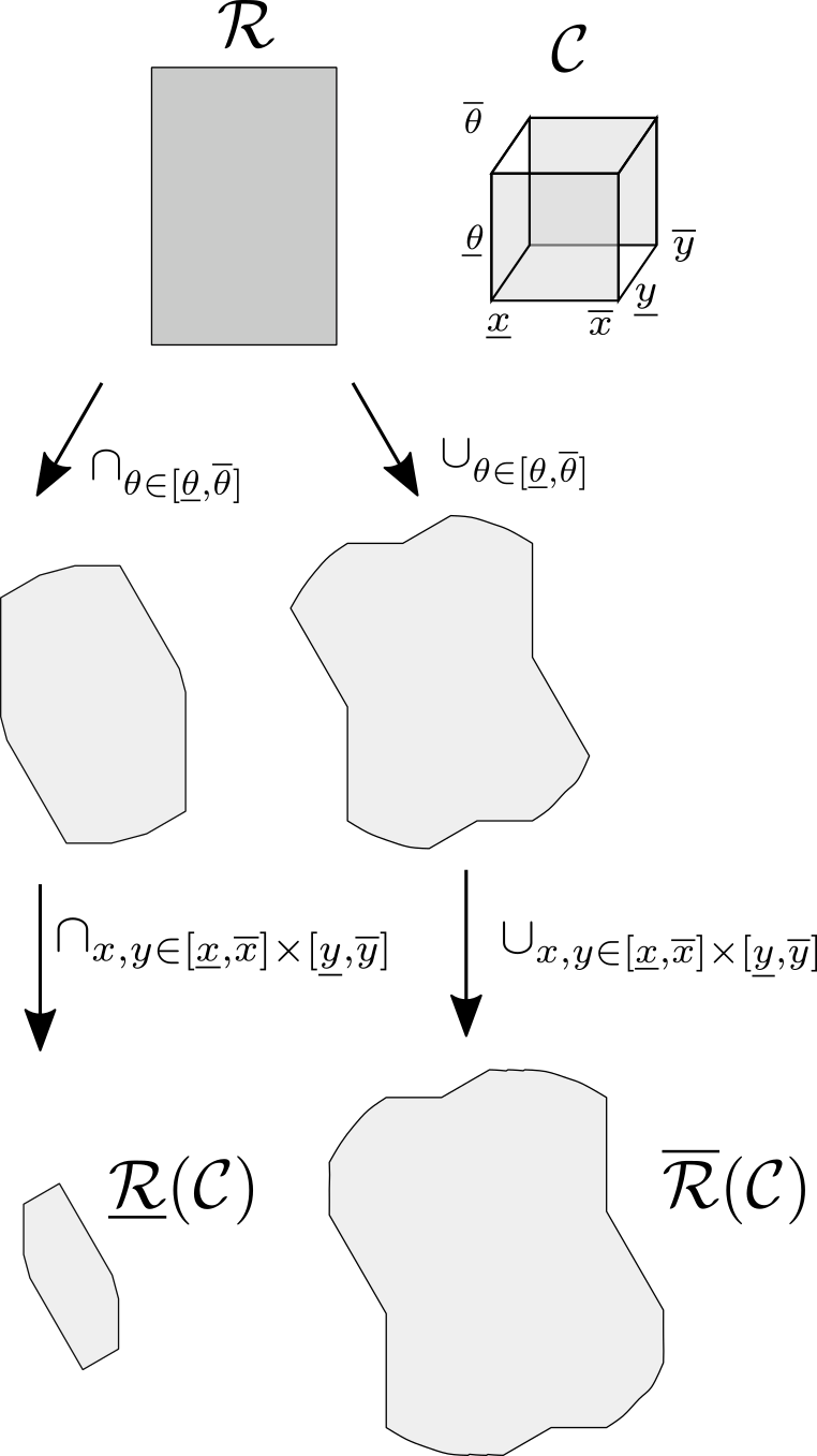
Figure 2: Under-approximation $\underline{\mathcal{R}}\left({\mathcal{C}}\right)$ (left) and over-approximation $\overline{\mathcal{R}}\left({\mathcal{C}}\right)$ (right) of a rectangular shaped robot corresponding to the configuration space cell $\mathcal{C}=[\underline{x},\overline{x}]\times[\underline{y},\overline{y}]\times[\underline{\theta},\overline{\theta}]$.

To do so, we propose the adaptive subdivision method outlined in Algorithm 2. Beginning with the state space cell defined by the Cartesian product of the axis-aligned bounding box of $\mathcal{W}$ and the set $\mathcal{Z}_{[q]}$, the proposed algorithm builds a partition $\mathcal{P}$ of the robot’s state space by adaptively subdividing cells that lie on its frontier $\mathcal{F}$. Specifically, at each iteration, a cell $(\mathcal{C}_{[p]},\mathcal{C}_{[q]})\in\mathcal{F}$ is selected and if $\overline{\mathcal{R}}\left({\mathcal{C}_{[p]}}\right)$ lies inside $\mathcal{W}$, then it is added to $\mathcal{P}$. Instead, if $\overline{\mathcal{R}}\left({\mathcal{C}_{[p]}}\right)$ overlaps with the complement of $\mathcal{W}$, then that cell gets discarded. If, at this point, the cell cannot be labeled either safe or unsafe and its size is not smaller than a user specified threshold $\epsilon_{w}$, then the cell gets subdivided and the new cells are added to the frontier $\mathcal{F}$. Otherwise, if the cell’s size is smaller than the specified threshold and cannot be subdivided any more, it is included in the partition $\mathcal{P}$. Finally, the desired over-approximation $\overline{\mathcal{Z}}_{s}$ can be obtained as the union of the cells in the computed partition $\mathcal{P}$.

In the following theorem we show that Algorithm 2 terminates in finite time and its worst case run-time is related to the size of the workspace and the reciprocal of the volume of the smallest allowable cell, as expected. Moreover, we show that the resulting cell partition $\mathcal{P}$ lies in the workspace and covers the robot’s entire safe set, exceeding it in proportion to a user-selected tolerance. Finally, we bound the possible safety violations that can result from the operation of the robot in $\mathcal{P}$. Specifically, we show that violations are proportional to the size of translation outside of $\mathcal{Z}_{s}$, but rotations outside of $\mathcal{Z}_{s}$ are amplified by the maximum distance from any point in the robot to its center of rotation.

Theorem 1.

Suppose a compact set $\mathcal{W}\subset\mathbb{R}^{2}$, a mapping $\mathcal{R}:\mathbb{R}^{2}\times[0,2\pi)\mapsto\mathfrak{S}(\mathbb{R}^{2})$, and $\epsilon_{w}>0$. Let also $\overline{\mathcal{R}},\underline{\mathcal{R}}:\mathfrak{S}(\mathbb{R}^{2}\times[0,2\pi))\mapsto\mathfrak{S}(\mathbb{R}^{2})$ be mappings satisfying Equation 7. Let $\mathcal{F}_{0}$ be the initialization of $\mathcal{F}$. Then Algorithm 2 terminates in finite time after at most $2\epsilon_{w}^{-3}\mathrm{vol}\left({\mathcal{F}_{0}}\right)$ repetitions of the while loop. It’s output, $\mathcal{P}$, is a collection of cells in $\mathcal{W}$ satisfying $\mathcal{Z}_{s}\subseteq\cup_{\mathcal{C}\in\mathcal{P}}\mathcal{C}\subseteq\mathcal{Z}_{s}\oplus(\mathcal{C}_{\epsilon_{w}}\times\mathrm{0})$.

Suppose further that $\mathcal{R}([x,y,\theta]^{\mathsf{T}})=R(\theta)\mathrm{R}+[x,y]^{\mathsf{T}}$, where $R(\theta)$ is a rotation in $\mathbb{R}^{2}$, and $\mathrm{R}\subseteq\mathcal{B}_{r}$ for some $r>0$. In this case, $\cup_{\mathcal{C}\in\mathcal{P}}\mathcal{C}\cup_{p\in\mathcal{C}_{[p]}}\mathcal{R}(p)\subseteq\mathcal{W}\oplus\mathcal{B}_{v}$ where $v=2r^{2}(1-\cos(\epsilon_{w}))+2\sqrt{2}\epsilon_{w}$.

Proof.

To begin, observe that all operations in Algorithm 2 are well-defined and can be computed in finite time due to the compactness assumption on $\mathcal{W}$ and the outputs of $\mathcal{R}$. All relevant set widths are finite due to this assumption.

To bound the while loop’s repetitions, observe that each repetition either: removes a cell from $\mathcal{F}$, reducing $\mathrm{vol}\left({\mathcal{F}}\right)$ by at least the minimum cell volume, $\epsilon_{w}^{3}$, or replaces one cell in $\mathcal{F}$ with two covering the same volume, leaving $\mathrm{vol}\left({\mathcal{F}}\right)$ unchanged, but increasing the number of cells by one. The maximum number of cells in $\mathcal{F}$ is bounded above by $k=\epsilon_{w}^{-3}\mathrm{vol}\left({\mathcal{F}_{0}}\right)$ because when $k$ cells are in $\mathcal{F}$, their the total volume is at least $k\epsilon_{w}^{3}$, but $\mathrm{vol}\left({\mathcal{F}}\right)$ can never grow. Hence, at most $k$ repetitions can add cells to $\mathcal{F}$, and $k$ can remove cells.

To verify that $\mathcal{Z}_{s}\subseteq\cup_{\mathcal{C}\in\mathcal{P}}\mathcal{C}$, suppose that it fails to hold. Then there exists $z\in\mathcal{Z}_{[p],s}$ where $z\notin\operatorname{\bigcup}_{\mathcal{C}\in\mathcal{P}}\mathcal{C}_{[p]}$. However, by design $z\in\operatorname{\bigcup}_{\mathcal{C}_{[p]}\in\mathcal{F}_{0}}\mathcal{C}_{[p]}$. This can only happen if a cell containing $z$, $\mathcal{C}_{[p]}$, was removed because $\underline{\mathcal{R}}\left({\mathcal{C}_{[p]}}\right)\not\subseteq\mathcal{W}$. This implies that for all $p\in\mathcal{C}_{[p]}$, $\mathcal{R}(p)\not\subseteq\mathcal{W}$. In particular, this must hold for $p=z$, contradicting the assumption that $z\in\mathcal{Z}_{[p],s}$.

To verify $\cup_{\mathcal{C}\in\mathcal{P}}\mathcal{C}\subseteq\mathcal{Z}_{s}\oplus(\mathcal{C}_{\epsilon_{w}}\times\mathrm{0})$, note that cells can only be added to $\mathcal{P}$ in two ways. First, $\mathcal{C}$ can be added if $\overline{\mathcal{R}}\left({\mathcal{C}_{[p]}}\right)\subseteq\mathcal{W}$, which implies $\mathcal{C}_{[p]}\subseteq\mathcal{Z}_{[p],s}$, and hence $\mathcal{C}\subseteq\mathcal{Z}_{s}\subset\mathcal{Z}_{s}\oplus(\mathcal{C}_{\epsilon_{w}}\times\mathrm{0})$. Otherwise, $\mathcal{C}$ can only be added if $\underline{\mathcal{R}}\left({\mathcal{C}_{[p]}}\right)\not\subseteq\mathcal{W}$ and GetMaxWidth($\mathcal{C}_{[p]}$) $>\epsilon_{w}$ fail to hold. These respectively imply that there exists $z\in\mathcal{C}_{[p]}\cap\mathcal{Z}_{[p],s}$ and that $\mathcal{C}_{[p]}\subseteq z\oplus\mathcal{C}_{\epsilon_{w}}\subseteq\mathcal{Z}_{[p],s}\oplus\mathcal{C}_{\epsilon_{w}}$, which means $\mathcal{C}\subseteq\mathcal{Z}_{s}\oplus(\mathcal{C}_{\epsilon_{w}}\times\mathrm{0})$.

For the final assertion, suppose $p\in\mathcal{C}_{[p]}$ for some $\mathcal{C}\in\mathcal{P}$. From the prior assertions, $p=[x,\theta]^{\mathsf{T}}+[\delta x,\delta\theta]^{\mathsf{T}}$, where $[x,\theta]^{\mathsf{T}}\in\mathcal{Z}_{[p],s}$ and $[\delta x,\delta\theta]^{\mathsf{T}}\in\mathcal{C}_{\epsilon_{w}}$. Therefore $\mathcal{R}(p)=R(\delta\theta)R(\theta)\mathrm{R}+x+\delta x$. Using the Cosine Rule and recalling that rotations preserve norms, $||x-R(\delta\theta)x||=2||x||^{2}(1-\cos(\delta\theta))\leq 2r^{2}(1-\cos(\epsilon_{w}))$ if $x\in R(\theta)\mathrm{R}$. Hence, $\mathcal{R}(p)\subseteq\mathcal{R}([x,\theta]^{\mathsf{T}})\oplus\mathcal{B}_{2r^{2}(1-\cos(\epsilon_{w}))}\oplus[-\epsilon_{w},\epsilon_{w}]^{2}$. Noting that $\mathcal{B}_{2r^{2}(1-\cos(\epsilon_{w}))}\oplus[-\epsilon_{w},\epsilon_{w}]^{2}\subseteq\mathrm{B}_{v}$ gives the desired result. ∎

Remark 1.

Note that Algorithm 2 does not produce a mathematical partition of $\overline{\mathcal{Z}}_{s}$ because the cells include their boundaries, where they may overlap. If one is needed, simple modifications can be made to the cell definition and subdivision algorithms to include boundaries in only one cell without fundamentally changing Algorithm 2.

1function $\mathcal{P}=$BuildPrtn($\mathcal{W},\mathcal{R},\epsilon_{w}$)

2       $\mathcal{P},\ \mathcal{F}\ \leftarrow\left\{{}\right\},\ \left\{\text{A bounded cell covering of }\mathcal{W}\right\}\times\mathbb{S}^{1}$ ;

3       while $\mathcal{F}$ is not empty 

4             $\mathcal{C}_{[p]}\ \leftarrow\text{a cell in }\mathcal{F}$ ;

5             $\mathcal{F}\ \leftarrow\ \mathcal{F}\setminus\mathcal{C}_{[p]}$;

6             if $\overline{\mathcal{R}}\left({\mathcal{C}_{[p]}}\right)\subseteq\mathcal{W}$ 

7                   $\mathcal{P}\leftarrow\mathcal{P}\cup\left\{{\mathcal{C}_{[p]}\times\mathcal{Z}_{[q]}}\right\}$

8            elseif $\underline{\mathcal{R}}\left({\mathcal{C}_{[p]}}\right)\subseteq\mathcal{W}$ 

9                   if MaxWidth($\mathcal{C}_{[p]}$)$<\epsilon_{w}$ 

10                         $\mathcal{F}\leftarrow\mathcal{F}\cup$SubdivideCell($\mathcal{C}_{[p]}$)

11                  else

12                         $\mathcal{P}\leftarrow\mathcal{P}\cup\left\{{\mathcal{C}_{[p]}\times\mathcal{Z}_{[q]}}\right\}$

13                  

14            

15      

Algorithm 2 Given a robot described by, $\mathcal{R}$, an allowable workspace, $\mathcal{W}$, and a tolerance, $\epsilon_{w}$, produce a cell collection, $\mathcal{P}$, covering $\overline{\mathcal{Z}}_{s}$ with bounded safety violations.

III-B Over-Approximation of the Forward Reachable Set of the Closed-Loop System

Using the over-approximation $\overline{\mathcal{Z}}_{s}$ of the robot’s safe state space as a set of initial robot states, in this section we employ reachability analysis techniques to compute an over-approximation of the forward reachable set of the closed loop system. Since the accuracy of the over-approximation of the forward reachable set depends on the partition $\mathcal{P}$ of the over-approximation of the safe set $\overline{\mathcal{Z}}_{s}$, we also propose a method to refine the partition $\mathcal{P}$ in order improve the accuracy of the over-approximation $\overline{\mathcal{Z}}_{c}$. This way we can control the tradeoff between computational complexity affected by the number of cells in $\mathcal{P}$ and accuracy of the over-approximation $\overline{\mathcal{Z}}_{c}$.

More specifically, to obtain a tight over-approximation of the set of states $\mathcal{Z}_{c}$ reachable from $\overline{\mathcal{Z}}_{s}$ using the robot’s closed-loop dynamics, we begin by noting that the partition constructed by Algorithm 2 consists of cells defined by $n$-dimensional intervals. As such, given a state space cell $\mathcal{C}\in\overline{\mathcal{Z}}_{s}$, the state space cell $\mathfrak{R}\left({\mathcal{C}}\right)$ reachable from $\mathcal{C}$ can be computed using $F$ defined in (2) which returns a bounding box enclosing the set of states reachable from $\mathcal{C}$ under the neural network controller, i.e.,

$$\mathfrak{R}\left({\mathcal{C};w,b}\right)=F\left({{\mathcal{C}},{\Phi\left({\mathcal{C};w,b}\right)}}\right)$$ (8)

where $\Phi$ is a continuous map of a $n$-dimensional interval to a $m$-dimensional interval such that

$$\phi\left({z;w,b}\right)\in\Phi\left({\mathcal{C};w,b}\right),~{}~{}~{}\forall z\in\mathcal{C}.$$ (9)

To obtain a function $\Phi$ that returns a valid over-approximation of the set of control inputs generated by the neural network $\phi$, we employ the Interval Bound Propagation (IBP) method [24]. In words, for each cell $\mathcal{C}\in\mathcal{P}$, we employ the IBP method (function $\Phi$) to compute bounds on the robot’s control inputs, which we then propagate (function $F$) to obtain bounds on the robot’s forward reachable set. Thus, the over-approximation $\overline{\mathcal{Z}}_{c}$ of the set of states reachable by the closed-loop system after one step can be obtained as

$$\overline{\mathcal{Z}}_{c}=\bigcup\limits_{\mathcal{C}\in\mathcal{P}}{\mathfrak{R}\left({\mathcal{C};w,b}\right)}.$$ (10)

We remark that the over-approximation error between the bounds on the control inputs computed using IBP and the actual bounds on the control inputs generated by $\phi$ for the states in $\mathcal{C}$ increases with the size of $\mathcal{C}$, as explained in [24]. Therefore, a fine partition $\mathcal{P}$ of the safe space over-approximation $\overline{\mathcal{Z}}_{s}$ is generally required in order to obtain a tight over-approximation of $\mathcal{Z}_{c}$. To refine $\mathcal{P}$ while keeping the total number of cells as low as possible, we further subdivide only cells whose forward reachable set intersects with the complement of $\overline{\mathcal{Z}}_{s}$. To identify such cells, we recall that the forward reachable set $\mathfrak{R}\left({\mathcal{C}}\right)$ of $\mathcal{C}$ is a composite interval with the same dimension as $\mathcal{C}$ and consider the two components $\mathcal{C}_{[p]}^{\prime}\in\mathcal{Z}_{[p]}$ and $\mathcal{C}_{[q]}^{\prime}\in\mathcal{Z}_{[q]}$ of $\mathfrak{R}\left({\mathcal{C}}\right)$ such that $\mathfrak{R}\left({\mathcal{C}}\right)=\mathcal{C}_{[p]}^{\prime}\times\mathcal{C}_{[q]}^{\prime}$. Following the procedure presented in subsection III-A, we can compute an over-approximation $\overline{\mathcal{R}}\left({\mathcal{C}_{[p]}^{\prime}}\right)$ of the robot’s footprint corresponding to the forward reachable set of configurations $\mathcal{C}_{[p]}^{\prime}$. Therefore, a cell $\mathcal{C}$ in $\mathcal{P}$ only needs to be subdivided if $\overline{\mathcal{R}}\left({\mathcal{C}_{[p]}^{\prime}}\right)$ intersects with the complement of the workspace $\mathcal{W}$ or $\mathcal{C}_{[q]}^{\prime}$ intersects with the complement $\mathrm{cmpl}\left({\mathcal{Z}_{[q]}}\right)$ of $\mathcal{Z}_{[q]}$.

1function $A=$PenaltyTest($\mathcal{C},\ \epsilon_{V_{p}},\ \epsilon_{V_{q}};\ \mathcal{W},\ \mathcal{R},\ \mathcal{Z}_{[q]},\ f$)

2       $A,\ \mathcal{C}^{\prime}\leftarrow$ false, $\mathfrak{R}\left({\mathcal{C}}\right)\$;

3       if $\mathrm{vol}\left({\overline{\mathcal{R}}\left({\mathcal{C}_{[p]}^{\prime}}\right)\cap\mathrm{cmpl}(\mathcal{W})}\right)>\epsilon_{V_{p}}\ \mathrm{\mathbf{or}}\ \mathrm{vol}\left({\mathcal{C}_{[q]}^{\prime}\cap\mathrm{cmpl}\left({\mathcal{Z}_{[q]}}\right)}\right)>\epsilon_{V_{q}}$ 

4             $A\ \leftarrow\$ true ;

5            

6      

Algorithm 3 Verify whether an outer approximation of the robot’s one-step reachable set violates safety requirements by more than margins $\epsilon_{V_{p}},\ \epsilon_{V_{q}}$ anywhere in cell $\mathcal{C}$.

1function $\mathcal{P}^{\prime}=$RefinePrtn($\mathcal{P},\ \epsilon_{w},\ \epsilon_{V_{p}},\ \epsilon_{V_{q}};\ \mathcal{W},\ \mathcal{R},\ \mathcal{Z}_{[q]},\ f$)

2       $\mathcal{F},\ \mathcal{P}^{\prime}\leftarrow\mathcal{P},\ \emptyset$ ;

3       while $\mathcal{F}$ is not empty 

4             $\mathcal{C}\ \leftarrow\text{a leaf cell in the last level of }\mathcal{F}$ that has not yet been examined;

5             if  PenaltyTest($\mathcal{C},\ \epsilon_{V_{p}},\ \epsilon_{V_{q}};\ \mathcal{W},\ \mathcal{R},\ \mathcal{Z}_{s},\ f$)  

6                  if MaxWidth($\mathcal{C}_{[p]}$)$>\epsilon_{w}$ 

                        $\mathcal{F}\leftarrow\mathcal{F}\cup\left(\text{{\sc SubdivideCell}($\mathcal{C}_{[p]}$)}\times\mathcal{C}_{[q]}\right)$ ;

                          // Children $\mathcal{C}$

7                        

8                  else

9                         $\mathcal{F}\ \leftarrow\ \mathcal{F}\setminus\mathcal{C}$ ;

10                        

11                  

12            else

13                  $\mathcal{C}^{sib},\ \mathcal{C}^{par}\leftarrow$ GetSibling($\mathcal{C}$), GetParent($\mathcal{C}$);

14                   if PenaltyTest($\mathcal{C}^{sib},\ \epsilon_{V_{p}},\ \epsilon_{V_{q}};\ \mathcal{W},\ \mathcal{R},\ \mathcal{Z}_{s},\ f$) 

15                         if MaxWidth($\mathcal{C}_{[p]}^{sib}$)$<\epsilon_{w}$ 

                              $\mathcal{F}\leftarrow\mathcal{F}\cup\left({\text{{\sc SubdivideCell}($\mathcal{C}_{[p]}^{sib}$)}\times\mathcal{C}_{[q]}^{sib}}\right)$ ;

                                // Children of $\mathcal{C}^{sib}$

16                              

17                        else

18                               $\mathcal{F}\ \leftarrow\ \mathcal{F}\setminus\mathcal{C}$ ;

19                              

20                        

21                  elseif  $\mathcal{C}^{sib}=\emptyset\ \mathrm{\mathbf{or}}$ CannotMerge($\mathcal{C},\mathcal{C}^{sib}$)  

22                         $\mathcal{F}\leftarrow(\mathcal{F}\setminus\{\mathcal{C},\mathcal{C}^{sib},\mathcal{C}_{par}\})$ ;

23                         $\mathcal{P}^{\prime}\leftarrow\mathcal{P}^{\prime}\cup\mathcal{C}\cup\mathcal{C}^{sib}$ ;

24                        

25                  else

                         $\mathcal{F}\leftarrow(\mathcal{F}\setminus\{\mathcal{C},\mathcal{C}^{sib},\mathcal{C}_{par}\})\cup$ Merge($\mathcal{C}^{sib},\mathcal{C}$) ;

                          // Replace $\mathcal{C}_{par}$

26                        

27                  

28            

29      

Algorithm 4 Refine $\mathcal{P}$ and remove cells where the robot’s one-step reachable set may violate safety requirements beyond specified tolerances.

The process described above is outlined in Algorithm 4 which adaptively subdivides cells in $\mathcal{P}$ with large over-approximation errors of their forward reachable sets. Specifically, for each cell $\mathcal{C}=(\mathcal{C}_{[p]},\mathcal{C}_{[q]})$ in $\mathcal{P}$, we check whether the area of $\mathrm{cmpl}(\mathcal{W})$ covered by $\overline{\mathcal{R}}\left({\mathcal{C}_{[p]}^{\prime}}\right)$ or the volume of $\mathrm{cmpl}\left({\mathcal{Z}_{[q]}}\right)$ covered by $\mathcal{C}_{[q]}^{\prime}$ are greater than user specified thresholds $\epsilon_{V_{p}}$ and $\epsilon_{V_{q}}$, respectively. If these conditions hold and the size of the cell admits further subdivision, then the cell gets split and replaced by smaller ones. Otherwise, the sibling $\mathcal{C}^{sib}$ of cell $\mathcal{C}$ is retrieved and if the volume of their parent cell $\mathcal{C}_{mrg}$ that lies outside the set of safe state $\mathcal{Z}_{s}$ is negligible, then the cells $\mathcal{C}$ and $\mathcal{C}^{sib}$ are merged in order to reduce the size of $\mathcal{P}$. Finally, the over-approximation $\overline{\mathcal{Z}}_{c}$ can be obtained as the union of the forward reachable set of each cell in $\mathcal{P}$. Algorithm 4 effectively controls the tradeoff between computational complexity affected by the number of cells in the partition $\mathcal{P}$ and accuracy of the over-approximation $\overline{\mathcal{Z}}_{c}$.

In the following theorem we show that Algorithm 4 terminates in finite time and its worst case run-time is related to the size of the workspace, the number of intervals in $\mathcal{Z}_{[q]}$, and the reciprocal of the volume of the smallest allowable cell. Moreover, we show that the resulting cell partition $\mathcal{P}^{\prime}$ inherits the safety assurances of $\mathcal{P}$ and that safety violations of its one-step reachable set are bounded by a user-specified tolerance.

Theorem 2.

Suppose Algorithm 2 is applied to a compact set $\mathcal{W}\subset\mathbb{R}^{2}$ and let $\mathcal{P}=\mathcal{P}_{[p]}\times\mathcal{Z}_{[q]}$ denote its output. Consider also the mapping $\mathcal{R}:\mathbb{R}^{2}\times[0,2\pi)\mapsto\mathfrak{S}(\mathbb{R}^{2})$, the tolerance $\epsilon_{w}>0$, and assume that the assumptions of Theorem 1 hold. Suppose that Algorithm 4 is applied to $\mathcal{P}$ with discrete-time forward dynamics governed by Equations 1-4 and tolerances $\epsilon_{V_{p}},\epsilon_{V_{q}}>0$. Then, Algorithm 4 terminates after $\#\left(\mathcal{Z}_{[q]}\right)\mathrm{vol}\left({\mathcal{P}_{[p]}}\right)\epsilon_{w}^{-3}$ repetitions of its while loop and the output, $\mathcal{P}^{\prime}$, satisfies $\cup_{\mathcal{C}\in\mathcal{P}^{\prime}}\mathcal{C}\subseteq\mathcal{Z}_{s}\oplus(\mathcal{C}_{\epsilon_{w}}\times\mathrm{0})$ and $\cup_{\mathcal{C}\in\mathcal{P}^{\prime}}\mathcal{C}\cup_{p\in\mathcal{C}_{[p]}}\mathcal{R}(p)\subseteq\mathcal{W}\oplus\mathrm{B}_{v}$. Moreover, if $\mathcal{C}^{\prime}=\mathfrak{R}\left({\mathcal{C}}\right)$ for $\mathcal{C}\in\mathcal{P}^{\prime}$, then $\mathrm{vol}\left({\overline{\mathcal{R}}\left({\mathcal{C}_{[p]}^{\prime}}\right)\cap\mathrm{cmpl}(\mathcal{W})}\right)\leq\epsilon_{V_{p}}$ and $\mathrm{vol}\left({\mathcal{C}_{[q]}^{\prime}\cap\mathrm{cmpl}\left({\mathcal{Z}_{[q]}}\right)}\right)\leq\epsilon_{V_{q}}$.

Proof.

Most assertions in this proof follow from observing that if $\mathcal{C}^{\prime}\in\mathcal{P}^{\prime}$, then $\mathcal{C}^{\prime}\subseteq\mathcal{C}\in\mathcal{P}$, and by following the arguments in the proof of Theorem 1. The bound on the one-step reachable set’s safety violations holds because cells are only added to $\mathcal{C}^{\prime}$ if Algorithm 3 returns false. Only the complexity bound requires additional discussion.

To establish the complexity bound, observe that for any cell $\mathcal{C}^{\prime}\in\mathcal{F}$, we have that $\mathcal{C}^{\prime}_{[p]}\subseteq\mathcal{C}_{p}\in\mathcal{P}_{[p]}$ and $\mathcal{C}^{\prime}_{[q]}=\mathcal{C}_{q}\in\mathcal{Z}_{[q]}$ because cells are only added to $\mathcal{F}$ by subdividing their configuration dimensions. For any interval $\mathcal{Z}\in\mathcal{Z}_{[q]}$, note that

$$V_{\mathcal{Z}}=\mathrm{vol}\left({\bigcup_{\mathcal{C}\in\mathcal{X}_{\mathcal{Z}}}\mathcal{C}_{[p]}}\right),$$

where $\mathcal{X}_{\mathcal{Z}}=\left\{\mathcal{C}\in\mathcal{F}|\text{{\sc IsLeaf}($\mathcal{C}$) = true, and }\mathcal{C}_{[q]}=\mathcal{Z}\right\}$ remains constant when cells are subdivided or merged, or decreases as cells are removed. Initially, $V_{\mathcal{Z}}=\mathrm{vol}\left({\mathcal{P}_{[p]}}\right)$ for all $\mathcal{Z}\in\mathcal{Z}_{[q]}$, which bounds $V_{\mathcal{Z}}$ above at all iterations. Observe that due to the subdivision operations, if $\mathcal{C}^{1},\mathcal{C}^{2}\in\mathcal{X}_{\mathcal{Z}}$, then $\mathcal{C}_{[p]}^{1}$, and $\mathcal{C}_{[p]}^{2}$ can only overlap on their boundaries. Then MaxWidth($\mathcal{C}_{[p]}$)$\geq\epsilon_{w}$ implies there can be at most $n_{\mathcal{Z}}=\mathrm{vol}\left({\mathcal{P}_{[p]}}\right)\epsilon_{w}^{-3}$ cells in $\mathcal{X}_{\mathcal{Z}}$, and subsequently at most $L_{max}=\#\left(\mathcal{Z}_{[q]}\right)\mathrm{vol}\left({\mathcal{P}_{[p]}}\right)\epsilon_{w}^{-3}$ leaves in $\mathcal{F}$. At each repetition of the while loop, a leaf cell, $\mathcal{C}\in\mathcal{F}$, is examined and one of the following happens:

• the number of leaves increases by one because $\mathcal{C}$ or its sibling is subdivided; or

• the number of leaves decreases by one or more because either $\mathcal{C}$, its sibling, and/or its parent are removed, or because $\mathcal{C}$ and its sibling are merged and replace their parent.

The required bound is found by observing that leaves can only be added at most $L_{max}$ times and removed at most $L_{max}$ times, which completes the complexity argument. ∎

III-C Safety-Aware Control Training

This section uses the over-approximation of the forward reachable set of the closed loop system $\overline{\mathcal{Z}}_{c}$, to design appropriate penalty terms which, when added to the loss function (6), minimize the overlap between this forward reachable set and the set of unsafe states. In this way, we can reduce safety violations after re-training of the neural network controller (3). To do so, we solve the following optimization problem at every iteration of Algorithm 1 to update the neural network parameters

$$\underset{w,b}{\text{minimize}} J^{\star}\left({w,b}\right)$$ (11)

$$J^{\star}\left({w,b}\right)=J\left({w,b}\right)+\lambda_{S}\cdot h\left({w,b}\right),$$ (12)

where $\lambda_{S}$ is a positive constant and $h$ a penalty term that measures safety violations. The goal in designing the penalty term $h$ is to push the over-approximation of the new forward reachable set $\overline{\mathcal{Z}}_{c}$ inside the under-approximation $\underline{\mathcal{Z}}_{s}=\cup_{\mathcal{C}\in\mathcal{P}_{S}}{\mathcal{C}}$ of the set of safe states $\mathcal{Z}_{s}$, where $\mathcal{P}_{S}$ denotes the subset of the partition $\mathcal{P}$ consisting of only safe cells. To do so, we define the penalty term $h$ as $\begin{aligned} h\left({w,b}\right)=\sum\nolimits_{\mathcal{C}^{\prime}\in\mathfrak{R}(\mathcal{P})}{V\left({\mathcal{C}^{\prime},\mathcal{P}_{S}}\right)}^{2},\end{aligned}$ where $\mathfrak{R}(\mathcal{P})=\left\{{\mathfrak{R}\left({\mathcal{C}}\right)~{}|~{}\mathcal{C}\in\mathcal{P}}\right\}$ and $V\left({\mathcal{C},\mathcal{P}_{S}}\right)$ is a valid metric of the volume occupied by the intersection of the composite interval $\mathcal{C}$ and $\cup_{\mathcal{C}\in\mathcal{P}_{S}}{\mathcal{C}}$. Thus, $h$ vanishes only if $\mathcal{C}^{\prime}\subseteq\cup_{\mathcal{C}\in\mathcal{P}_{S}}{\mathcal{C}}$ for all $\mathcal{C}^{\prime}\in\mathfrak{R}(\mathcal{P})$, i.e., the set of safe states is rendered invariant under the closed-loop dynamics. Note that the overlap between the forward reachable set and the set of unsafe states $\mathcal{Z}_{c}\setminus\mathcal{Z}_{s}$ also provides numerical bounds on possible safety violations by the closed loop system, that can be used as a measure of reliability of the neural network controller (3).

IV Numerical Experiments

In this section, we illustrate the proposed method through numerical experiments involving a rectangular shaped robot that operates inside the workspace depicted in Figure 3.

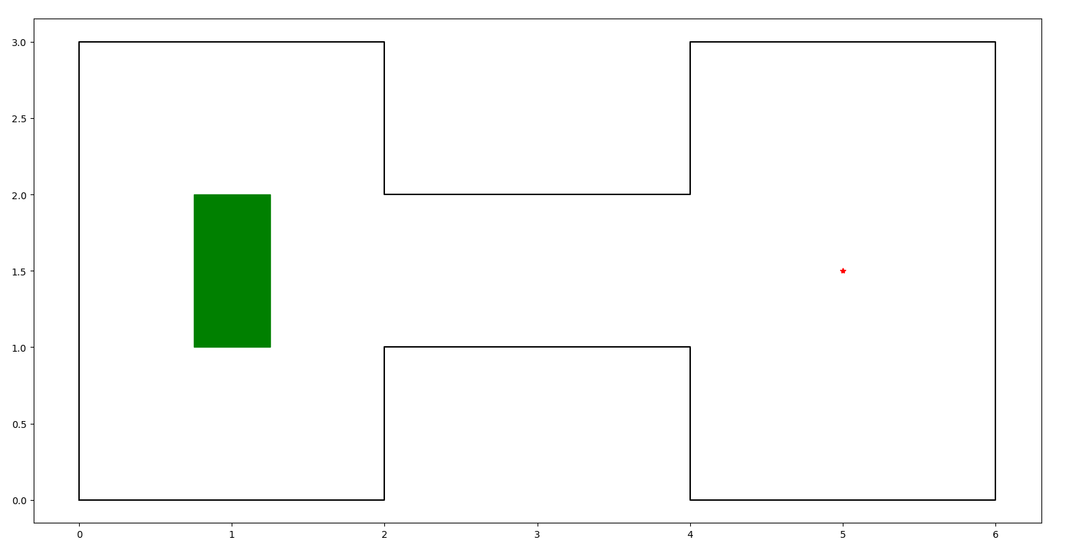
Figure 3: Workspace, consisting of two rooms and a corridor, and the robot’s body at default orientation (green rectangle). The desired position of the robot’s reference point is placed at the room on the right (red point).

The robot is assumed to be holonomic obeying the simple kinematic model

$$z_{k+1}=z_{k}+K\cdot\phi\left({z_{k}}\right),$$ (13)

with $z=p$ and $K=0.01$. The dataset $\mathcal{D}$ was assembled by computing 500 feasible trajectories using the RRT^⋆ algorithm [29] and initializing the robot at random configurations. Particularly, each point $(z,u)\in\mathcal{D}$ corresponds to a sampled trajectory point $(z,u^{\prime})$, where the control input $u^{\prime}$ is modified to ensure that the implicitly defined vector field vanishes at the goal configuration, i.e.,

$$u=10\cdot\frac{u^{\prime}}{\|u^{\prime}\|}\frac{\|z^{\star}-z\|}{1-\|z^{\star}-z\|}.$$ (14)

The over-approximation of the robot’s forward reachable set for a given cell $\mathcal{C}$ is computed as the Minkowski sum between that cell and the controller’s output reachable set for that cell, i.e.,

$$F\left({{\mathcal{C}},{\Phi\left({\mathcal{C}}\right)}}\right)=\mathcal{C}\oplus\left({K\cdot\Phi\left({\mathcal{C}}\right)}\right).$$ (15)

Additionally, the metric $V$ used in the evaluation of the penalty term $h$ is defined by

$$V\left({\mathcal{C},\mathcal{P}_{S}}\right)=\left({\mathrm{vol}_{\delta}\left({\mathcal{C}}\right)}\right)^{1/3}-\left({\sum_{\mathcal{C}^{\prime}\in\mathcal{P}_{S}}{\mathrm{vol}_{\delta}\left({\mathcal{C}\cap\mathcal{C}^{\prime}}\right)}}\right)^{1/3},$$ (16)

where $\delta=[\delta_{x}=1,\delta_{y}=1,\delta_{\theta}=1/2\pi]$ are constant scaling factors. Particularly, the cubic root of the volume of composite intervals in (16) is used because, in practice, it prevents terms corresponding to slim cells from vanishing too fast when, e.g., only one of their dimensions has grown small whereas the others have not. The scaling factors $\delta_{x},\delta_{y},\delta_{\theta}$ allow to assign different weights to each dimension, given that they have incompatible units ($x$ and $y$ are in meters and $\theta$ is given in rad).

NN	Shape	$\epsilon_{w}$	Partition Size
			Initial	Refined
$\phi_{1}$	3x50x50x50x3	(0.1, 0.1, 0.2$\pi$)	5434	6990
$\phi_{2}$	3x50x50x50x3	(0.25, 0.25, 0.2$\pi$)	1046	1180
$\phi_{3}$	3x50x50x3	(0.1, 0.1, 0.2$\pi$)	5434	5536

TABLE I: Shape and subdivision thresholds used in the re-training of each neural network controller, along with the number of cells in the corresponding partitions $\mathcal{P}$ after their construction and initial refinement.

NN	$\lambda_{S}$		$J(w,b)$
	Step Size	Final Value	Initial Value	Final Value
$\phi_{1}$	$1.0e{-4}$	$5.0e{-3}$	3.4200	3.6659
$\phi_{2}$	$2.0e{-4}$	$1.0e{-2}$	3.4200	3.6114
$\phi_{3}$	$4.0e{-5}$	$2.0e{-3}$	3.5345	3.7948

TABLE II: Step size and final value of the penalty coefficient $\lambda_{S}$ as well as the value of the loss function $J$ before and after re-training for each respective neural network controller.

Three separate neural network controllers $\phi_{1},\phi_{2},\phi_{3}$ with various shapes were trained to safely steer the robot to the desired configuration using the proposed methodology using different values for the subdivision threshold $\epsilon_{w}$. The activation functions of the hidden layers of all three neural network controllers were selected to be hyperbolic tangent functions. The shapes of these neural networks and the values of the subdivision thresholds $\epsilon_{w}$ used for safe training of each controller can be seen in Table I. Also, the parameters $\lambda_{B}$ and $\lambda_{R}$ in (6) were set to $1/|\mathcal{D}|$ and $1/(|w|+|b|)$, respectively, with $|\mathcal{D}|$ denoting the number of data points in $\mathcal{D}$ and $|w|,|b|$ denoting the dimension of the corresponding neural network controller’s weight and bias vectors. After initially training each network using the data in $\mathcal{D}$, we used Algorithm 2 to obtain an initial partition $\mathcal{P}$ of the robot’s configuration space with the subdivision threshold $\epsilon_{w}=\left({{\epsilon_{w}}_{x},{\epsilon_{w}}_{y},{\epsilon_{w}}_{\theta}}\right)$ for each respective dimension. Then, we applied Algorithm 4 to refine the initial partition $\mathcal{P}$ based on the system’s forward reachable sets with $\epsilon_{V_{p}}=1e-2$. The number of cells in the partition $\mathcal{P}$ associated with each neural network controller before and after the first refinement can be seen in Table I. We remark that blindly partitioning the configuration space $\mathcal{W}\times\mathbb{S}^{1}$ into cells with dimensions $0.1\times 0.1\times 0.2\pi$ would result in $14000$ cells or more, which implies that the proposed method requires $1-6990/14000\approx 50\%$ and $1-5536/14000\approx 60\%$ less subdivisions for the cases of $\phi_{1}$ and $\phi_{3}$, respectively. Among these cells, the active ones (i.e., cells whose forward reachable sets violate the safety specifications) were used to evaluate the penalties at each iteration. Finally, 50 iterations of the refinement and parameter update steps of Algorithm 1 were performed. Similarly to the approach proposed in [20] where the size of the $\epsilon$-neighborhoods was gradually increased to improve numerical stability of the retraining procedure, the parameter $\lambda_{S}$ in (12) was initialized at $0$ and its value was increased at the beginning of each iteration of Algorithm 1 until a target value was reached at the 50th iteration. The selected step size and the corresponding target value of the parameter $\lambda_{S}$ used in the re-training of each controller are listed in Table II.

Figure 4 shows the evolution of the total volume of $\overline{\mathcal{Z}}_{c}$ lying outside the under-approximation of the set of safe states, which is given by $\mathcal{P}_{S}$, i.e., $\mathrm{vol}\left({\left({\cup_{\mathcal{C}\in\mathcal{P}}{\mathfrak{R}\left({\mathcal{C}}\right)}}\right)\cap\left({\cup_{\mathcal{C}\in\mathcal{P}_{S}}{\mathcal{C}}}\right)}\right)$ whereas Figure 5 depicts the number of active cells at the end of each epoch, with epoch $0$ corresponding to the initial training of the controllers ($\lambda_{S}=0$). After re-training, the volume of $\bar{\mathcal{Z}}_{c}$, which bounds the volume of initial states that may escape the safe set under the closed-loop dynamics, and the number of active cells decreased by $84.6\%,54.4\%,30.9\%,$ and $31.6\%,15.3\%,9.5\%$, respectively, for each of the three neural network controllers. Additionally, the values of the loss function $J$ before the first epoch and after the last one are listed in Table II. We note that in all three cases the value of the loss function $J$ increases, which is to be expected as the proposed framework prioritizes safety over liveliness of the neural network controller.

The projections of the cells in each partition onto the $xy$-plane along with the over-approximations of their forward reachable sets before and after retraining can be seen in Figure 6-Figure 8. We remark that the area covered by the over-approximation of the robot’s forward reachable set (colored in red) that lies outside the set of initial states (colored in blue) has noticeably decreased at the end of $50$-th epoch, especially for the case of the neural network controller $\phi_{1}$. This area provides spatial bounds on possible safety violations induced by the trained controllers. As a result, while our method allows for safety violations, it does so with grace, by providing such bounds that can be controlled during training. Finally, several trajectories executed by the robot equipped with the controller $\phi_{1}$ before and after 50 iterations of re-training are illustrated in Figure 9. As can be seen in subfigure 9(a), the proposed re-training method results in safer robot trajectories than the ones returned by the initially trained neural network controller, whereas the behavior of the closed-loop system at states away from the boundary of the safe set is not noticeably affected, as indicated by subfigure 9(b).

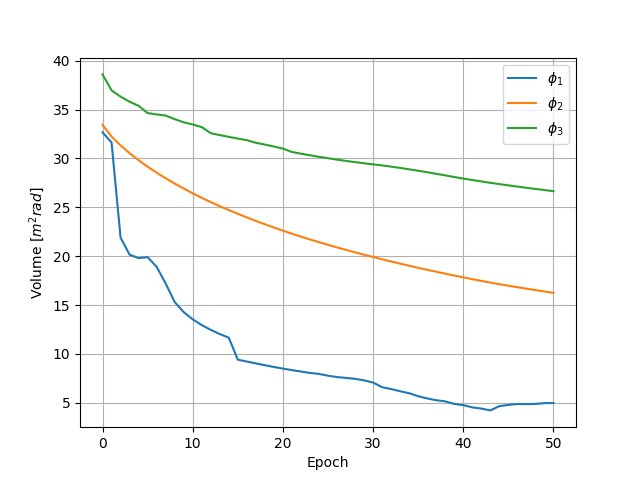
Figure 4: Total volume of active cells that lies outside the set of safe states at the beginning of each epoch.

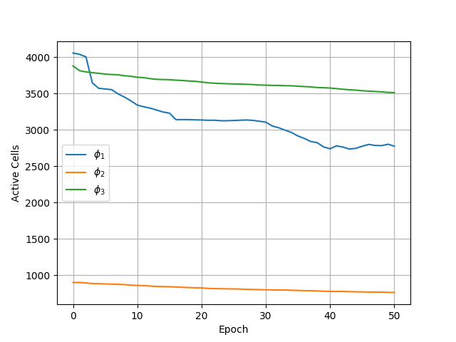
Figure 5: Number of active cells at the beginning of each epoch.

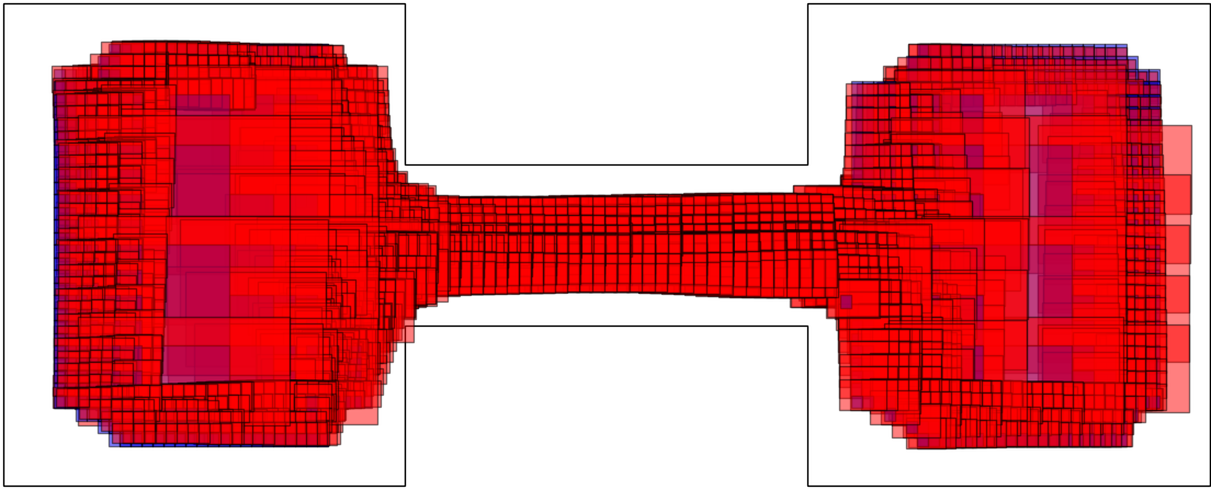
(a) $\phi_{1}$: Before re-training

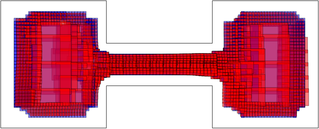
(b) $\phi_{1}$: After re-training

Figure 6: Projections of cells (blue boxes) of partition corresponding to neural network controller $\phi_{1}$ onto the $xy$-plane overlayed with the over-approximations of their forward reachable sets (red boxes) before and after retraining.

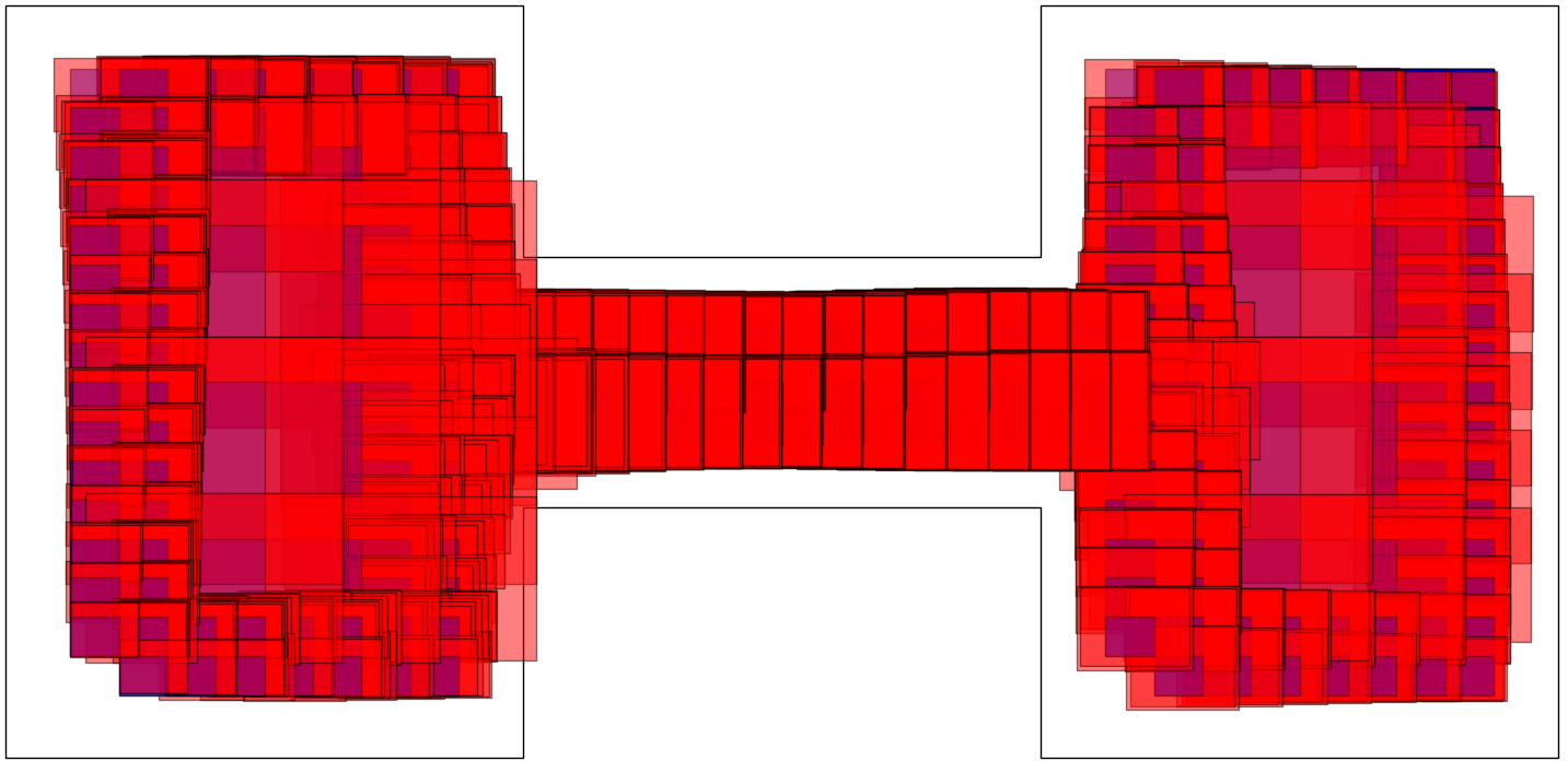
(a) $\phi_{2}$: Before re-training

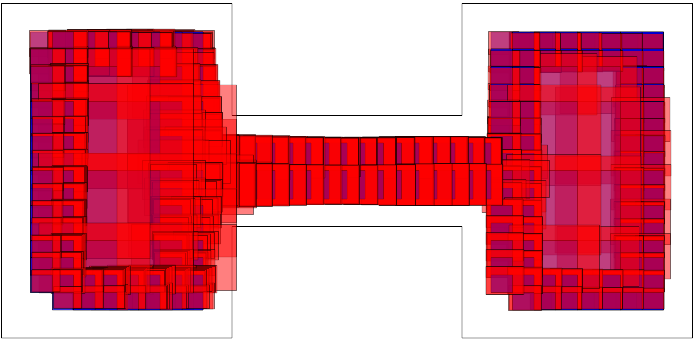
(b) $\phi_{2}$: After re-training

Figure 7: Projections of cells (blue boxes) of partition corresponding to neural network controller $\phi_{2}$ onto the $xy$-plane overlayed with the over-approximations of their forward reachable sets (red boxes) before and after retraining.

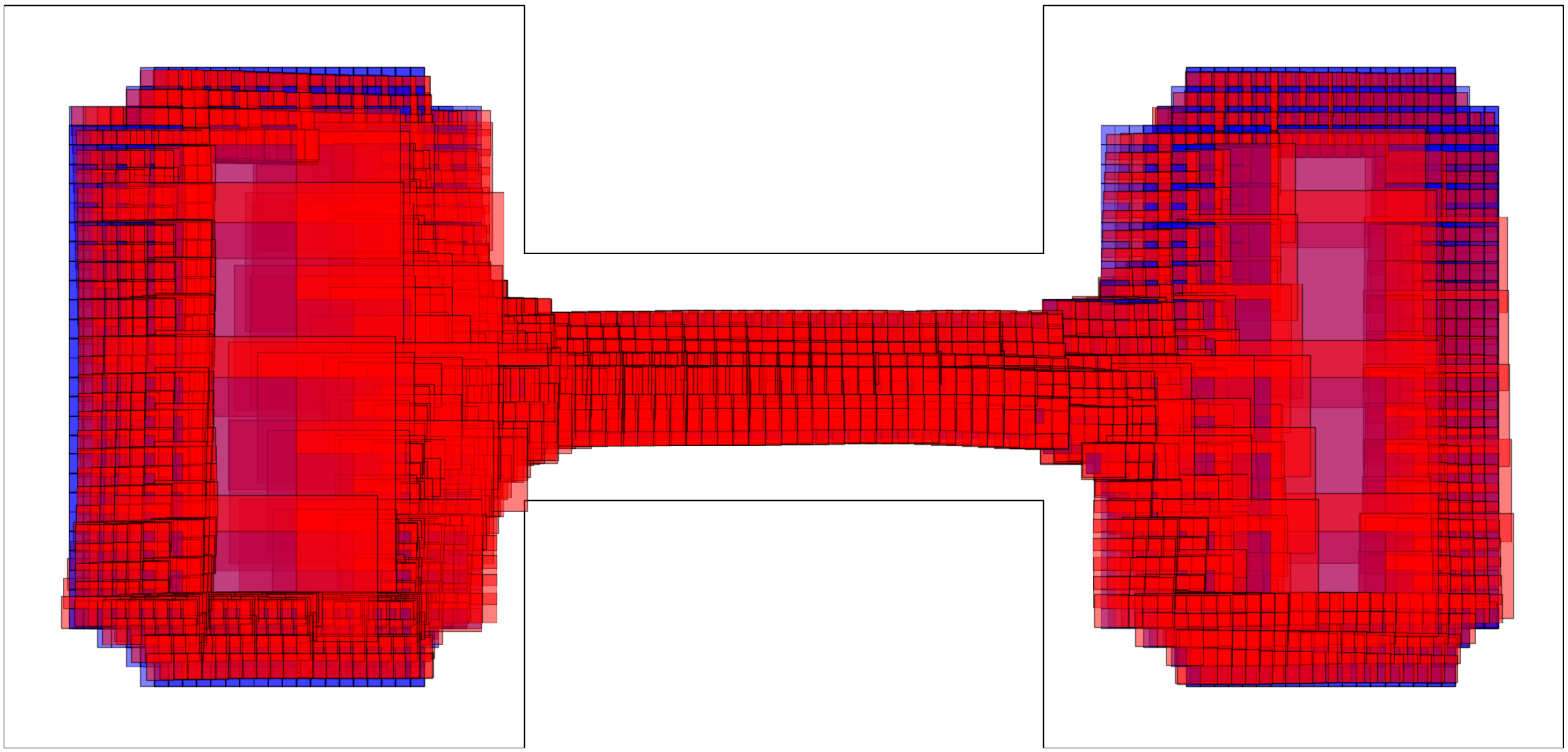
(a) $\phi_{3}$: Before re-training

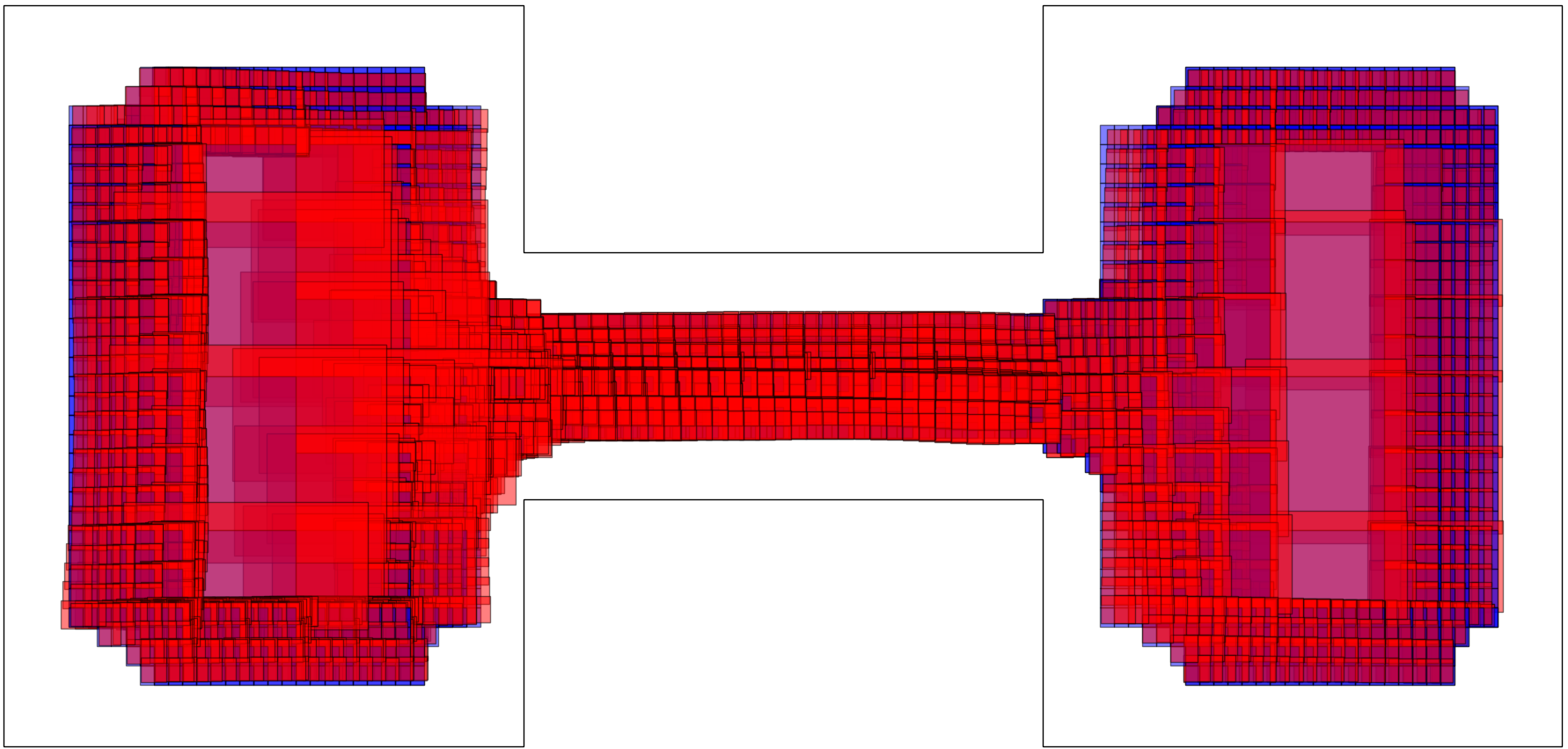
(b) $\phi_{3}$: After re-training

Figure 8: Projections of cells (blue boxes) of partition corresponding to neural network controller $\phi_{3}$ onto the $xy$-plane overlayed with the over-approximations of their forward reachable sets (red boxes) before and after retraining.

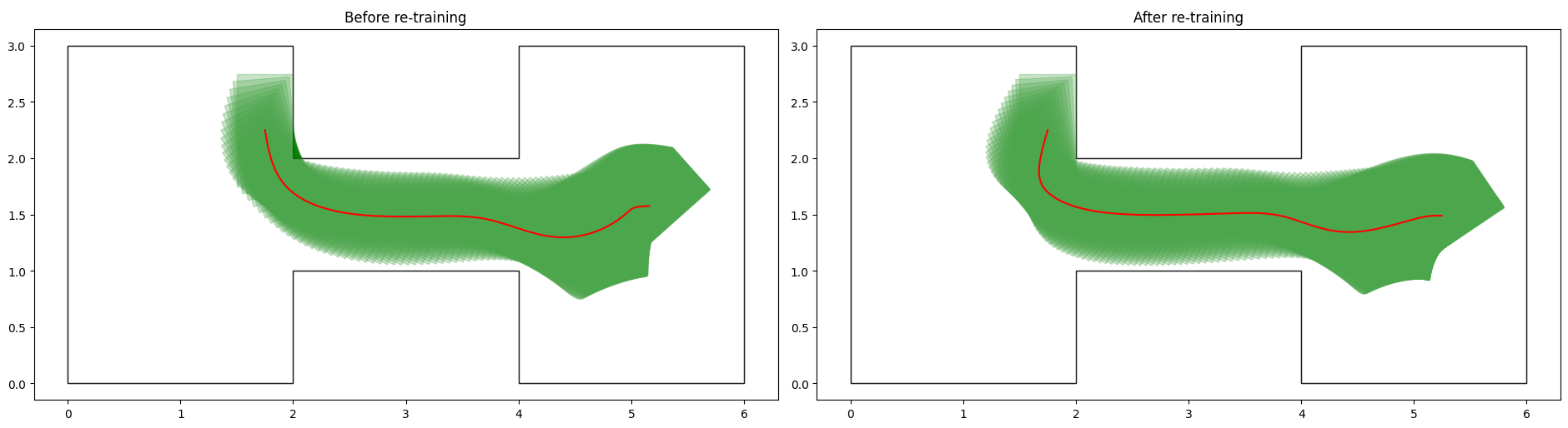
(a)

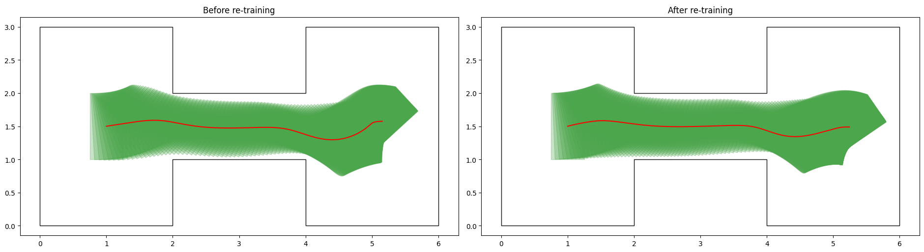
(b)

Figure 9: Trajectories of the robot starting from various configurations before and after re-training of the controller $\phi_{1}$. The path traversed by the robot’s reference point is depicted in red and the body of the robot at various configurations is shown in green.

V Conclusions

In this work, we addressed the problem of safely steering a polygonal robot operating inside a compact workspace to a desired configuration using a feed-forward neural network controller trained to avoid collisions between the robot and the workspace boundary. Compared to existing methods that depend strongly on the density of data points close to the boundary of the safe state space to train neural network controllers with closed-loop safety guarantees, our approach lifts such strong assumptions on the data that are hard to satisfy in practice and instead allows for graceful safety violations, i.e., of a bounded magnitude that can be spatially controlled.

References

- [1] A. Amini, G. Rosman, S. Karaman, and D. Rus, “Variational end-to-end navigation and localization,” in 2019 International Conference on Robotics and Automation (ICRA), 2019, pp. 8958–8964.
- [2] F. Shamsfakhr and B. S. Bigham, “A neural network approach to navigation of a mobile robot and obstacle avoidance in dynamic and unknown environments,” SSRN Electronic Journal, 2020. [Online]. Available: https://doi.org/10.2139/ssrn.3619573
- [3] T. Nageli, J. Alonso-Mora, A. Domahidi, D. Rus, and O. Hilliges, “Real-time motion planning for aerial videography with dynamic obstacle avoidance and viewpoint optimization,” IEEE Robotics and Automation Letters, vol. 2, no. 3, pp. 1696–1703, 2017. [Online]. Available: https://doi.org/10.1109/lra.2017.2665693
- [4] Y. F. Chen, M. Everett, M. Liu, and J. P. How, “Socially aware motion planning with deep reinforcement learning,” in 2017 IEEE/RSJ International Conference on Intelligent Robots and Systems (IROS), 2017, pp. 1343–1350.
- [5] V. Schmuck and D. Meredith, “Training networks separately on static and dynamic obstacles improves collision avoidance during indoor robot navigation,” in ESANN 2019 - Proceedings, 27th European Symposium on Artificial Neural Networks, Computational Intelligence and Machine Learning, M. Verleysen, Ed. ESANN, Apr. 2019, pp. 655–660, european Symposium on Artificial Neural Networks, Computational Intelligence and Machine Learning, ESANN ; Conference date: 24-04-2019 Through 26-04-2019. [Online]. Available: https://www.elen.ucl.ac.be/esann/
- [6] T. Perkins and A. Barto, “Lyapunov design for safe reinforcement learning control,” J. Mach. Learn. Res., vol. 3, pp. 803–, 05 2003.
- [7] P. Geibel and F. Wysotzki, “Risk-sensitive reinforcement learning applied to control under constraints,” J. Artif. Int. Res., vol. 24, no. 1, p. 81–108, Jul. 2005.
- [8] X. Li and C. Belta, “Temporal logic guided safe reinforcement learning using control barrier functions,” 2019. [Online]. Available: https://arxiv.org/abs/1903.09885
- [9] M. Ohnishi, L. Wang, G. Notomista, and M. Egerstedt, “Barrier-certified adaptive reinforcement learning with applications to brushbot navigation,” IEEE Transactions on Robotics, vol. 35, no. 5, pp. 1186–1205, 2019. [Online]. Available: https://doi.org/10.1109/tro.2019.2920206
- [10] R. Cheng, G. Orosz, R. M. Murray, and J. W. Burdick, “End-to-end safe reinforcement learning through barrier functions for safety-critical continuous control tasks,” Proceedings of the AAAI Conference on Artificial Intelligence, vol. 33, pp. 3387–3395, 2019. [Online]. Available: https://doi.org/10.1609/aaai.v33i01.33013387
- [11] A. Robey, H. Hu, L. Lindemann, H. Zhang, D. V. Dimarogonas, S. Tu, and N. Matni, “Learning control barrier functions from expert demonstrations,” 2020. [Online]. Available: https://arxiv.org/abs/2004.03315
- [12] L. Lindemann, H. Hu, A. Robey, H. Zhang, D. V. Dimarogonas, S. Tu, and N. Matni, “Learning hybrid control barrier functions from data,” 2020. [Online]. Available: https://arxiv.org/abs/2011.04112
- [13] A. Bajcsy, S. Bansal, E. Bronstein, V. Tolani, and C. J. Tomlin, “An efficient reachability-based framework for provably safe autonomous navigation in unknown environments,” 2019. [Online]. Available: https://arxiv.org/abs/1905.00532
- [14] J. F. Fisac, A. K. Akametalu, M. N. Zeilinger, S. Kaynama, J. Gillula, and C. J. Tomlin, “A general safety framework for learning-based control in uncertain robotic systems,” 2018. [Online]. Available: https://arxiv.org/abs/1705.01292
- [15] A. Li, S. Bansal, G. Giovanis, V. Tolani, C. Tomlin, and M. Chen, “Generating robust supervision for learning-based visual navigation using hamilton-jacobi reachability,” 2020. [Online]. Available: https://arxiv.org/abs/1912.10120
- [16] G. Katz, C. Barrett, D. Dill, K. Julian, and M. Kochenderfer, “Reluplex: An efficient smt solver for verifying deep neural networks,” 2017. [Online]. Available: https://arxiv.org/abs/1702.01135
- [17] W. Ruan, X. Huang, and M. Kwiatkowska, “Reachability analysis of deep neural networks with provable guarantees,” 2018. [Online]. Available: https://arxiv.org/abs/1805.02242
- [18] S. Dutta, S. Jha, S. Sanakaranarayanan, and A. Tiwari, “Output range analysis for deep neural networks,” 2017. [Online]. Available: https://arxiv.org/abs/1709.09130
- [19] H. Zhang, T.-W. Weng, P.-Y. Chen, C.-J. Hsieh, and L. Daniel, “Efficient neural network robustness certification with general activation functions,” 2018. [Online]. Available: https://arxiv.org/abs/1811.00866
- [20] H. Zhang, H. Chen, C. Xiao, S. Gowal, R. Stanforth, B. Li, D. Boning, and C.-J. Hsieh, “Towards stable and efficient training of verifiably robust neural networks,” 2019. [Online]. Available: https://arxiv.org/abs/1906.06316
- [21] S. Dutta and S. Sankaranarayanan, “Reachability analysis for neural feedback systems using regressive polynomial rule inference,” in ACM International Conference on Hybrid Systems: Computation and Control, 04 2019, pp. 157–168.
- [22] C. Huang, J. Fan, W. Li, X. Chen, and Q. Zhu, “Reachnn: Reachability analysis of neural-network controlled systems,” 2019. [Online]. Available: https://arxiv.org/abs/1906.10654
- [23] H. Hu, M. Fazlyab, M. Morari, and G. J. Pappas, “Reach-sdp: Reachability analysis of closed-loop systems with neural network controllers via semidefinite programming,” 2020. [Online]. Available: https://arxiv.org/abs/2004.07876
- [24] W. Xiang, H.-D. Tran, and T. T. Johnson, “Output reachable set estimation and verification for multi-layer neural networks,” 2018. [Online]. Available: https://arxiv.org/abs/1708.03322
- [25] W. Xiang, H.-D. Tran, X. Yang, and T. T. Johnson, “Reachable set estimation for neural network control systems: A simulation-guided approach,” 2020. [Online]. Available: https://arxiv.org/abs/2004.12273
- [26] M. Everett, G. Habibi, and J. P. How, “Robustness analysis of neural networks via efficient partitioning with applications in control systems,” 2020. [Online]. Available: https://arxiv.org/abs/2010.00540
- [27] D. J. Zhu and J. . Latombe, “New heuristic algorithms for efficient hierarchical path planning,” IEEE Transactions on Robotics and Automation, vol. 7, no. 1, pp. 9–20, Feb 1991.
- [28] X. Sun and Y. Shoukry, “Provably correct training of neural network controllers using reachability analysis,” 2021. [Online]. Available: https://arxiv.org/abs/2102.10806
- [29] S. Karaman and E. Frazzoli, “Incremental sampling-based algorithms for optimal motion planning,” 2010. [Online]. Available: https://arxiv.org/abs/1005.0416