Winding number dependence of quantum vortex energies at one-loop

Abstract

We compute the one-loop vacuum polarization energies of Abrikosov-Nielsen-Olesen (ANO) vortices with topological charge $n$ in scalar electrodynamics, for the BPS case of equal gauge and scalar masses. This calculation allows us to investigate the relationship between the winding number and the quantum-corrected vortex energy, which in turn determines the stability of higher winding configurations against decay into configurations with unit winding. While the classical energy is proportional to $n$, we find that the vacuum polarization energy is negative and approximately proportional to $n-1$ with a small constant offset.

I Introduction

In scalar electrodynamics with spontaneous symmetry breaking, the Abrikosov-Nielsen-Olesen (ANO) vortex Abrikosov (1957a, b); Nielsen and Olesen (1973) is an axially symmetric configuration with topological soliton structure in the transverse plane. In the regular gauge, the fields vanish at the center and the winding number $n$ counts the mapping of the phase of the complex scalar field at spatial infinity onto the unit circle. This winding number, which we take to be positive throughout, corresponds to a quantized magnetic flux running along the string.

From the perspective of particle physics, we can view this solution as the analog in two space dimensions of a ’t Hooft-Polyakov magnetic monopole ’t Hooft (1974); Polyakov (1974). So-called cosmic string solutions can also emerge from a U(1) subgroup of the SU(2) weak interactions Vachaspati (1992); Achucarro and Vachaspati (2000); Nambu (1977); Hindmarsh and Kibble (1995); Kibble (1976); Shellard and Vilenkin (1994). Here the scalar field is the scalar Higgs doublet while the gauge fields are the massive vector bosons $W^{\pm}$ and $Z^{0}$. In condensed matter physics, these vortices represent the penetration of magnetic flux through a superconductor with the scalar field being the condensate order parameter. The ANO model is characterized by the ratio of the charged scalar mass to the effective mass acquired by the gauge field through spontaneous symmetry breaking. The inverses of these masses correspond to the superconducting coherence length and the London penetration depth respectively, where the former reflects the attractive self-interaction of the condensate of Cooper pairs, while the latter corresponds to the exponential Meissner suppression of electromagnetic fields in the condensate, leading to superconductivity Tinkham (1996).

The Bogomolny-Prasad-Sommerfeld (BPS) Bogomolny (1976); Prasad and Sommerfield (1975) case, in which the masses of the gauge and scalar fields are equal, is of particular interest because the classical mass is proportional to the winding number. As a result, the quantum correction to the classical energy, however small, determines whether higher winding number configurations are energetically stable against decay into vortices with unit winding. Our investigation provides the first nontrivial calculation of vacuum polarization energy (VPE) quantum corrections for a topological soliton with varying winding number in four spacetime dimensions.

In the scattering theory formalism, topological effects are captured in the behavior of the phase shift in the presence of zero-mode and threshold bound states, as expressed by Levinson’s theorem and its generalizations to situations with topological boundary conditions Niemi and Semenoff (1985); Boyanovsky and Blankenbecler (1985); Graham and Jaffe (1999); Farhi et al. (2001). Since Levinson’s theorem compares the phase shift at threshold to the phase shift at infinite wave number, it captures the effects of the soliton’s global topology at short distance. For gauge theory solitons in three space dimensions, such as the ANO vortex and ’t Hooft-Polyakov monopole one encounters a generalization of this behavior; making the gauge field go to zero at large distances, as is required for the scattering theory assumption of asymptotically free interactions, necessarily introduces singularities in the gauge field at the origin. These singularities disappear in gauge-invariant quantities, however, so that the soliton has finite energy density everywhere.

These singularities require the subtraction of quantities that formally vanish in the scattering theory calculation, but in practice cancel quadratically divergent contributions in intermediate results Graham and Weigel (2020). This subtraction enforces the cancellation of the superficial quadratic divergence of the gauge vacuum polarization, leaving only the logarithmic divergence, which is then accounted for through standard renormalization. This subtlety was first addressed in Ref. Baacke and Kevlishvili (2008) using an ad-hoc subtraction, while the more recent work in Ref. Graham and Weigel (2020) provides a simpler and more systematic algorithm for ensuring gauge invariance, which also leads to more reliable numerical results. A key test of the validity of this approach is that it renders the result insensitive to the choice of a minimal radius in the scattering calculation; one cannot numerically extend all the way to the origin because the gauge fields diverge there, but the subtracted quantities remain well-behaved in that limit, reflecting the absence of singularities in measurable quantities.

In the case of string solutions like the ANO vortex these subtleties can be further obfuscated by the slow convergence of the sum over partial waves. As a result, with insufficient numerical computation unrenormalized quantities can appear finite Pasipoularides (2001), meaning that the effects of renormalization will make them appear to diverge, when the true calculation shows the opposite behavior. In this work, we use the technical formulation established in Ref. Graham and Weigel (2020) combined with the “fake boson” formalism Farhi et al. (2002) to precisely subtract Born approximations to the scattering data that can then be added back in as renormalized Feynman diagrams implementing a modified on-shell renormalization scheme.

II ANO Vortices

The classical vortices are constructed from the Lagrangian of scalar electrodynamics

$$\mathcal{L}=-\frac{1}{4}F_{\mu\nu}F^{\mu\nu}+|D_{\mu}\Phi|^{2}-\frac{\lambda}{4}\left(|\Phi|^{2}-v^{2}\right)^{2}\,,$$ (1)

where $F_{\mu\nu}=\partial_{\mu}A_{\mu}-\partial_{\nu}A_{\mu}$ and $D_{\mu}\Phi=\left(\partial_{\mu}-{\rm i}eA_{\mu}\right)\Phi$.

The vortex profiles in the singular gauge are

$$\Phi_{S}=vh(\rho)\qquad{\rm and}\qquad{\boldsymbol{A}}_{S}=nv\hat{{\boldsymbol{\varphi}}}\,\frac{g(\rho)}{\rho}$$ (2)

where $\rho=evr$ is dimensionless while $r$ is the physical coordinate. The winding number $n$ is the essential topological quantity. In the BPS case with $\lambda=2e^{2}$, the energy functional is minimized when the profile functions obey the first-order differential equations

$$g^{\prime}=\frac{\rho}{n}(h^{2}-1)\qquad{\rm and}\qquad h^{\prime}=\frac{n}{\rho}gh\,.$$ (3)

and the boundary conditions

$$h(0)=1-g(0)=0\hbox{~{}and~{}}\lim_{\rho\to\infty}h(\rho)=1-\lim_{\rho\to\infty}g(\rho)=1\,.$$ (4)

Numerical solutions are displayed in Fig.1. The resulting energy is then proportional to the winding number, $E_{\rm cl}=2\pi nv^{2}$.

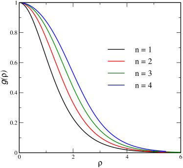
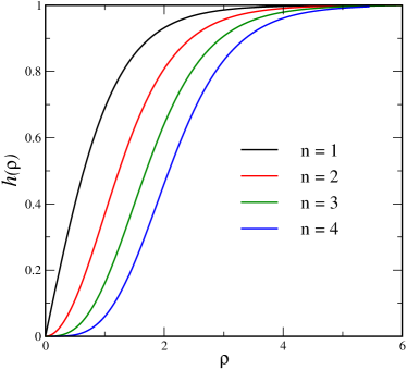
Figure 1: (color online) Classical profile functions of the vortex profile functions for the BPS case.

III Quantum Theory

To quantize the theory we introduce fluctuations about the vortex via

$$\Phi=\Phi_{S}+\eta\qquad{\rm and}\qquad A^{\mu}=A_{S}^{\mu}+a^{\mu}$$ (5)

and extract the harmonic terms in the fluctuations $\eta$ and $a^{\mu}$. The gauge is fixed by adding an $R_{\xi}$ type Lagrangian that cancels the $\eta\partial_{\mu}a^{\mu}$ and $\eta^{\ast}\partial_{\mu}a^{\mu}$ terms,

$$\mathcal{L}_{\rm gf}=-\frac{1}{2}\left[\partial_{\mu}a^{\mu}+{\rm i}e\left(\Phi_{S}\eta^{\ast}-\Phi_{S}^{\ast}\eta\right)\right]^{2}\,.$$ (6)

We still have to account for ghost contribution to the VPE associated with this gauge fixing, $\mathcal{L}_{\rm gf}=-\frac{1}{2}G^{2}$. The infinitesimal gauge transformations reads

$$A^{\mu}\to A^{\mu}+\partial\chi\,,\qquad\Phi_{S}+\eta\to\Phi_{S}+\eta+{\rm i}e\chi(\Phi_{S}+\eta)$$ (7)

so that $\eta\to\eta+{\rm i}e\chi(\Phi_{S}+\eta)\,.$ Then

$$\frac{\partial G}{\partial\chi}\Big{|}_{\chi=0}=\partial_{\mu}\partial^{\mu}+e^{2}\left(2|\Phi_{S}|^{2}+\Phi_{S}\eta^{\ast}+\Phi_{S}^{\ast}\eta\right)\,.$$ (8)

This induces the ghost Lagrangian Lee and Min (1995); Rebhan et al. (2004)

$$\mathcal{L}_{\rm gh}=\overline{c}\left(\partial_{\mu}\partial^{\mu}+2e^{2}|\Phi_{S}|^{2}\right)c+\mbox{non-harmonic terms}\,.$$ (9)

The corresponding VPE is that of a Klein Gordon field with mass $\sqrt{2}ev$ in the background potential $2v^{2}(h^{2}-1)$, which must be subtracted with a factor of negative two from the VPE obtained for the gauge and scalar fields. Since $D_{0}\Phi_{S}=0$ and $D_{3}\Phi_{S}=0$, the temporal and longitudinal components $a_{0}$ and $a_{3}$ fully decouple, contributing

$$-\frac{1}{2}\left[\partial_{\mu}a_{0}\partial^{\mu}a^{0}+\partial_{\mu}a_{3}\partial^{\mu}a^{3}\right]+|\Phi_{S}|^{2}\left[a_{0}a^{0}+a_{3}a^{3}\right]$$

to the Lagrangian. These fluctuations are subject solely to the background potential $2(|\Phi_{S}|^{2}-v^{2})$, which is exactly the same as that of the ghosts. As a result, the non-transverse and ghost contributions to the VPE cancel each other. Of course, this just reflects the fact that the free electromagnetic field only has two degrees of freedom.

After canceling the non-transverse gauge fluctuations against the ghost contribution, we end up with the truncated Lagrangian

$$\mathcal{L}^{(2)} =\frac{1}{2}\sum_{n=1,2}\left(\partial_{\mu}a_{n}\right)\left(\partial^{\mu}a_{n}\right)-e^{2}|\Phi_{S}|^{2}\sum_{n=1,2}a_{n}^{2}$$ (10)

$$\hskip 14.22636pt+|\dot{\eta}|^{2}-|\partial_{3}\eta|^{2}+\sum_{n=1,2}(D_{n}\eta)^{\ast}(D^{n}\eta)$$ (11)

$$\hskip 14.22636pt-e^{2}\left[3|\Phi_{S}|^{2}-v^{2}\right]|\eta|^{2}$$ (12)

$$\hskip 14.22636pt+2{\rm i}e\sum_{n=1,2}a_{n}\left[\eta^{\ast}\left(D^{n}\Phi_{S}\right)-\eta\left(D^{n}\Phi_{S}\right)^{\ast}\right]\,.$$ (13)

Essentially we have simplified the quantum gauge theory to that of four real scalar fields: $a_{1}$, $a_{2}$, ${\sf Re}(\eta)$ and ${\sf Im}(\eta)$.

IV Vacuum polarization energy

To compute the VPE we will employ spectral methods Graham:2009zz based on the scattering theory for quantum fluctuations about the potential induced by the vortex. To formulate the scattering problem, we employ a partial wave decomposition using the complex combinations

$$a_{+}=\sqrt{2}{\rm i}{\rm e}^{-{\rm i}\omega t}\sum_{\ell}a_{\ell}(\rho){\rm e}^{{\rm i}\ell\varphi}\hbox{~{}and~{}}\eta={\rm e}^{-{\rm i}\omega t}\sum_{\ell}\eta_{\ell}(\rho){\rm e}^{{\rm i}\ell\varphi}$$ (14)

and similarly for $a_{-}$ and $\eta^{\ast}$, leading to a $4\times 4$ scattering problem for the radial functions. For profile functions obeying Eq. (3), this problem decouples into two $2\times 2$ systems, with the one for $a_{-}$ and $\eta^{\ast}$ being the same as that of $a_{+}$ and $\eta$. Hence is suffices to compute the VPE of the latter and double it. The scattering problem is set up in terms of the Jost solution $\mathcal{F}_{\ell}$ by introducing

$$\begin{pmatrix}\eta^{(1)}_{\ell}&\eta^{(2)}_{\ell}\cr a^{(1)}_{\ell+1}&a^{(2)}_{\ell+1}\end{pmatrix}=\mathcal{F}_{\ell}\cdot\mathcal{H}_{\ell}\,,\mathcal{H}_{\ell}=\begin{pmatrix}H^{(1)}_{\ell}(q\rho)&0\cr 0&H^{(1)}_{\ell+1}(q\rho)\end{pmatrix}\,,$$ (15)

where the superscripts on the left-hand side refer to the two possible scattering channels when imposing the boundary condition $\lim_{\rho\to\infty}\mathcal{F}_{\ell}=\mbox{{\sf 1}\mbox{}\rule{0.39993pt}{6.6736pt}\mbox{\hskip 1.00006pt}}$. The Hankel functions $H^{(1)}$ parameterize outgoing cylindrical waves. In matrix form, the scattering differential equations for (dimensionless) imaginary momentum $t={\rm i}\sqrt{\omega^{2}-2e^{2}v^{2}}/(ev)^{2}$ read

$$\frac{\partial^{2}}{\partial\rho^{2}}\mathcal{F}_{\ell}=-\frac{\partial}{\partial\rho}\mathcal{F}_{\ell}-2\left(\frac{\partial}{\partial\rho}\mathcal{F}_{\ell}\right)\cdot\mathcal{Z}_{\ell}+\frac{1}{\rho^{2}}\left[\mathcal{L}_{\ell},\mathcal{F}_{\ell}\right]+\mathcal{V}_{\ell}\cdot\mathcal{F}_{\ell}\,.$$ (16)

The angular momenta enter via the logarithmic derivative matrix for the analytically continued Hankel functions

$$\mathcal{Z}_{\ell}=\begin{pmatrix}\frac{|l|}{\rho}-t\,\frac{K_{|l|+1}(t\rho)}{K_{|l|}(t\rho)}&0\cr 0&\frac{|l+1|}{\rho}-t\,\frac{K_{|l+1|+1}(t\rho)}{K_{|l+1|}(t\rho)}\end{pmatrix}$$ (17)

and

$$\mathcal{L}_{\ell}=\begin{pmatrix}\ell^{2}&0\cr 0&(\ell+1)^{2}\end{pmatrix}\,,$$ (18)

and the potential matrix is

$$\mathcal{V}_{\ell}=\begin{pmatrix}3(h^{2}(\rho)-1)+\frac{n^{2}g^{2}(\rho)-2n\ell g(\rho)}{\rho^{2}}&\sqrt{2}d(\rho)\cr\sqrt{2}d(\rho)&2(h^{2}(\rho)-1)\end{pmatrix}\,.$$ (19)

We then use Eq. (16) to compute the Jost function, which is given by $\nu_{\ell}(t)=\lim_{\rho\to 0}{\rm ln}\,{\rm det}\left[\mathcal{F}_{\ell}\right]$.

The standard procedure to determine the Born approximations, which are needed to regularize the ultraviolet divergences, fails when $g(0)\neq 0$. To perform the Born subtractions without the singular terms, we introduce

$$\overline{\mathcal{V}}=\begin{pmatrix}3(h^{2}(\rho)-1)&\sqrt{2}d(\rho)\cr\sqrt{2}d(\rho)&2(h^{2}(\rho)-1)\end{pmatrix}$$ (20)

and iterate

$$\frac{\partial^{2}}{\partial\rho^{2}}\overline{\mathcal{F}}_{\ell}=-\frac{\partial}{\partial\rho}\overline{\mathcal{F}}_{\ell}-2\left(\frac{\partial}{\partial\rho}\overline{\mathcal{F}}_{\ell}\right)\cdot\mathcal{Z}_{\ell}+\frac{1}{\rho^{2}}\left[\mathcal{L}_{\ell},\overline{\mathcal{F}}_{\ell}\right]+\overline{\mathcal{V}}\cdot\overline{\mathcal{F}}_{\ell}$$ (21)

according to the expansion $\overline{\mathcal{F}}_{\ell}=\mbox{{\sf 1}\mbox{}\rule{0.39993pt}{6.6736pt}\mbox{\hskip 1.00006pt}}+\overline{\mathcal{F}}_{\ell}^{(1)}+\overline{\mathcal{F}}_{\ell}^{(2)}+\ldots$, where the superscript refers to the order of $\overline{\mathcal{V}}$. From the derivation in Ref. Graham and Weigel (2020) we expect that

$$\left[\nu(t)\right]_{V} =\lim_{\genfrac{}{}{0.0pt}{}{L\to\infty}{\rho_{\rm min}\to 0}}\left\{\sum_{\ell=-L}^{L}\left[\nu_{\ell}(t)-\overline{\nu}^{(1)}_{\ell}(t)-\overline{\nu}^{(2)}_{\ell}(t)\right]_{\rho_{\rm min}}\right.$$

$$\left.\qquad-n^{2}\int_{\rho_{\rm min}}^{\infty}\frac{d\rho}{\rho}\,g^{2}(\rho)\right\}$$ (22)

approaches $\displaystyle\frac{n^{2}}{12t^{2}}\int_{0}^{\infty}\frac{d\rho}{\rho}\,\left(\frac{dg(\rho)}{d\rho}\right)^{2}$ as $t\to\infty$.

The subtraction of the integral in Eq. (22) cancels the superficial quadratic divergence in the VPE. By this subtraction we restore gauge invariance. The full computation of the VPE requires us to multiply the subtracted Jost function by $t$, capturing the effect of the translation-invariant direction, and integrate Graham et al. (2001). The right-hand side of Eq. (22) then leads to the logarithmic divergence associated with gauge field renormalization. This divergence is most conveniently treated within the fake boson formalism Farhi et al. (2002) which takes advantage of the fact that the second-order Born term for a scalar field also induces a logarithmic divergence. To be precise, we consider scattering of a boson about the potential $V_{f}=3e^{2}v^{2}(\tanh^{2}(\kappa evr)-1)$, for which $\overline{\nu}^{(2)}_{\ell}(t)$ is the second-order contribution to the Jost function on the imaginary momentum axis. We take $\kappa$ as a free parameter to later test our numerical simulation, since the final result for VPE should not depend on a particular choice. This subtraction is calibrated by defining

$$c_{B} = -\frac{e^{2}}{6}\frac{\int_{0}^{\infty}rdr\,F_{\mu\nu}F^{\mu\nu}}{\int_{0}^{\infty}rdrV_{f}^{2}}$$ (23)

$$= -\frac{n^{2}}{3}\frac{\int_{0}^{\infty}\rho d\rho\left(\frac{g^{\prime}(\rho)}{\rho}\right)^{2}}{\int_{0}^{\infty}\rho d\rho\,\left[3(\tanh^{2}(\kappa\rho)-1)\right]^{2}}$$ (24)

so that the scattering contribution to the VPE is

$$E_{\rm VPE}^{\rm scat.}=\frac{1}{2\pi}\int_{\sqrt{2}}^{\infty}tdt\,\left[\left[\nu(t)\right]_{V}-c_{B}\overline{\nu}^{(2)}(t)\right]\,.$$ (25)

To identify the subtraction in Eq. (25) in terms of Feynman diagrams Becchi et al. (1975); Irges and Koutroulis (2017) we consider the Lagrangian with four real fields $\phi^{\rm t}=(\eta_{1},\eta_{2},a_{1},a_{2})$

$$\mathcal{L}=\frac{1}{2}\left(\partial_{\mu}\phi^{\rm t}\right)\left(\partial^{\mu}\phi\right)-\frac{1}{2}\phi^{\rm t}M^{2}\phi-\phi^{\rm t}V\phi\,,$$ (26)

where $M=\sqrt{2}ev$ is the mass of both the gauge and scalar field fluctuations. The Cartesian components of the gauge fields have been defined above, and $\eta=\left(\eta_{1}+{\rm i}\eta_{2}\right)/\sqrt{2}$. The potential matrix is given by $V=V_{0}+V_{1}+V_{2}$ with

$$V_{0}=\begin{pmatrix}\frac{3\lambda}{4}\left(\Phi^{2}_{S}-v^{2}\right)&0&\sqrt{2}e^{2}\,\hat{{\boldsymbol{x}}}\cdot{\boldsymbol{A}}_{S}\Phi_{S}&\sqrt{2}e^{2}\,\hat{{\boldsymbol{y}}}\cdot{\boldsymbol{A}}_{S}\Phi_{S}\\[2.84526pt] 0&\frac{3\lambda}{4}\left(\Phi^{2}_{S}-v^{2}\right)&-\sqrt{2}e\,\hat{{\boldsymbol{x}}}\cdot{\boldsymbol{\nabla}}\Phi_{S}&-\sqrt{2}e\,\hat{{\boldsymbol{y}}}\cdot{\boldsymbol{\nabla}}\Phi_{S}\\[2.84526pt] \sqrt{2}e^{2}\,\hat{{\boldsymbol{x}}}\cdot{\boldsymbol{A}}_{S}\Phi_{S}&-\sqrt{2}e\,\hat{{\boldsymbol{x}}}\cdot{\boldsymbol{\nabla}}\Phi_{S}&e^{2}\left(\Phi^{2}_{S}-v^{2}\right)&0\\[2.84526pt] \sqrt{2}e^{2}\,\hat{{\boldsymbol{y}}}\cdot{\boldsymbol{A}}_{S}\Phi_{S}&-\sqrt{2}e\,\hat{{\boldsymbol{y}}}\cdot{\boldsymbol{\nabla}}\Phi_{S}&0&e^{2}\left(\Phi^{2}_{S}-v^{2}\right)\end{pmatrix}\,,$$ (27)

and

$$V_{1}=e\begin{pmatrix}0&1&0&0\\[0.0pt] -1&0&0&0\\[0.0pt] 0&0&0&0\\[0.0pt] 0&0&0&0\end{pmatrix}\,{\boldsymbol{A}}_{S}\cdot{\boldsymbol{\nabla}}$$ (28)

and

$$V_{2}=\frac{e^{2}}{2}\begin{pmatrix}1&0&0&0\\[0.0pt] 0&1&0&0\\[0.0pt] 0&0&0&0\\[0.0pt] 0&0&0&0\end{pmatrix}\,{\boldsymbol{A}}_{S}\cdot{\boldsymbol{A}}_{S}$$ (29)

Here we have separated out $V_{1}$ and $V_{2}$ since they relate to the singular terms in the scattering problem, while $V_{0}$ is the $4\times 4$ representation of $\overline{\mathcal{V}}$. The renormalization program via Feynman diagrams in dimensional regularization is carried out with the full potential matrix $V$, while the subtractions should only involve $V_{0}$ supplemented by the wave-function renormalization of the gauge boson, which in turn is simplified by the fake boson trick.

To form the diagrammatic expansion, we Taylor expand the effective action $\frac{{\rm i}}{2}{\rm Tr}\left[\partial^{2}+M^{2}+2V\right]$ for the four real scalar fields. The contribution linear in $V_{0}$ is the scalar tadpole and corresponds to the subtraction of $\overline{\nu}_{\ell}^{(1)}$ in Eq. (22). This tadpole diagram is fully canceled by a counterterm proportional to $\int d^{4}x\,\left(|\Phi|^{2}-v^{2}\right)$. The terms quadratic in $V_{0}$ correspond to $\overline{\nu}_{\ell}^{(2)}$ in Eq. (22) and are logarithmically divergent. These divergences are canceled by counterterms proportional to $\int d^{4}x\,\left(|\Phi|^{2}-v^{2}\right)^{2}$ and $\int d^{4}x\,|D_{\mu}\Phi|^{2}$. The contributions linear in $V_{2}$ and quadratic in $V_{1}$ combine such that the individual quadratic divergences cancel and the subleading logarithmic divergence matches that of the right hand side of Eq. (22). The logarithmic divergences from $V_{0}\otimes V_{2}$ and $V_{0}\otimes V_{1}\otimes V_{1}$ cancel, as do those from $V_{2}\otimes V_{2}$, $V_{2}\otimes V_{1}\otimes V_{1}$ and $V_{1}\otimes V_{1}\otimes V_{1}\otimes V_{1}$, so the subtractions discussed after Eq. (29) are sufficient to regularize the theory.

We implement a modified on-shell renormalization condition to fix the finite parts of the counterterms. For example, the Feynman diagram from two insertions of $\left(\Phi^{2}_{S}-v^{2}\right)$ and the corresponding counterterm combine to a four-dimensional momentum space integral of the form

$$\int\frac{d^{4}k}{(2\pi)^{4}}\,\widetilde{v}_{H}(k)\widetilde{v}_{H}(-k)G_{V}(k^{2})$$

with

$$G_{V}(k^{2})=\int_{0}^{1}dx\,{\rm ln}\left[1-x(1-x)\frac{k^{2}}{M^{2}}\right]+c_{V}\,.$$

Here $\widetilde{v}_{H}(k)$ is the Fourier transform of $\Phi^{2}_{S}-v^{2}$ and $c_{V}$ is the finite part of the counterterm coefficient. The modified on-shell renormalization condition then adjusts $c_{V}$ such that $G_{V}(M^{2})=0$. That is, there is no quantum correction to the location and residue of the pole due to the fluctuations. There are analogous conditions for the counterterms $\int d^{4}x\,|D_{\mu}\Phi|^{2}$ and $\int d^{4}x\,F_{\mu\nu}F^{\mu\nu}$. To simpify the calculation, we choose conditions such that the mass of the gauge particle is unchanged, meaning the masses remain equal at one-loop order. This choice comes at the cost of introducing a correction to the residue of the pole. An additional wavefunction renormalization to eliminate this correction, as would be necessary to compare to a physical system, would introduce a shift in the gauge mass. However, the effect of this shift only affects the VPE at higher loop orders. Collecting these terms, the finite counterterm contribution to the VPE is

$$\frac{E^{(0)}_{\rm CT}}{e^{2}v^{2}} =\int_{0}^{\infty}\rho d\rho\left\{\frac{n^{2}}{144}\left(\frac{16}{\pi}-3\sqrt{3}\right)\frac{g^{\prime 2}}{\rho^{2}}\right.$$ (30)

$$\hskip 7.11317pt\left.+\left(\frac{1}{\pi}-2\sqrt{3}\right)\left[h^{\prime 2}+\frac{n^{2}}{\rho^{2}}h^{2}g^{2}+\frac{13}{8}\left(1-h^{2}\right)^{2}\right]\right\}\,.$$

The Feynman diagram contribution arising from two insertions of $V_{0}$ is straightforward. We define Bessel-Fourier transforms

$$I_{A}(k) = \int_{0}^{\infty}dr\,h(\rho)g(\rho)J_{1}(kr)$$ (31)

$$I_{H}(k) = k\int_{0}^{\infty}rdr\,\left[1-h(\rho)\right]J_{0}(kr)$$ (32)

$$\widetilde{v}(k) = \int_{0}^{\infty}rdr\,\left[{h}^{2}(\rho)-1\right]J_{0}(kr)\,,$$ (33)

where $\rho=evr$, and obtain

$$\frac{E_{V_{0}}}{e^{2}v^{2}} = \int_{0}^{\infty}\frac{kdk}{2\pi}\left[n^{2}I^{2}_{A}(k)+I^{2}_{H}(k)+\frac{13e^{2}v^{2}}{8}\widetilde{v}^{2}(k)\right]$$ (35)

$$\times\int_{0}^{1}dx\,{\rm ln}\left[1+x(1-x)\frac{k^{2}}{M^{2}}\right]\,.$$

Finally, recall that we did not subtract the singular Born terms in Eq. (25) but rather the fake boson analog. Hence we require the Feynman diagram energy

$$E_{\rm fb}=\frac{c_{B}}{16\pi}\int_{0}^{\infty}kdk\,\widetilde{V}_{f}^{2}(k){\rm ln}\left[1+x(1-x)\frac{k^{2}}{M^{2}}\right]$$

with $\widetilde{V}_{f}(k)=3\int_{0}^{\infty}rdr\,\left[\tanh^{2}(\kappa\rho)-1\right]J_{0}(kr)$, corresponding to the fake boson potential. Then $E^{(0)}_{\rm FD}=E_{V_{0}}+E_{\rm fb}$ completes our expression for the VPE per unit length of the vortex,

$$E_{\rm VPE}=E^{\rm scat.}_{\rm VPE}+E^{(0)}_{\rm FD}+E^{(0)}_{\rm CT}\,.$$ (36)

V Numerical results for the VPE

The numerical treatment is hampered by slow convergence due to the logarithmic behavior of the subtracted Jost solution around the center of the vortex and of $\left[\nu(t)\right]_{V}$ at small $t$. The detailed solutions to these problems will be presented elsewhere Graham and Weigel (2021). One must also use a sum up to a large number of partial waves $L$ together with an asymptotic extrapolation to obtain accurate results for the sum over partial waves Graham and Weigel (2020).

$n=1$ $n=2$ $n=3$ $n=4$ $E^{(0)}_{\rm CT}$ 0.0370 0.0786 0.1214 0.1651 $E^{(0)}_{\rm FD}$ 0.0424 0.0315 0.0317 0.0335 0.0795 0.1101 0.1531 0.1986 $E^{\rm scat.}_{\rm VPE}$ -0.0510 -0.1939 -0.3563 -0.5251 $E_{\rm VPE}$ 0.0284 -0.0837 -0.2033 -0.3257

Table 1: Various contributions to and the total VPE for different winding numbers $n$. The fake boson potential is $V_{f}=3[\tanh^{2}(\kappa\rho)-1]$ with $\kappa=1,0.9,0.8,0.7$ for $n=1,2,3,4$, respectively. The third line contains the sum of the corresponding entries of the first two lines. All data are in units of $ev$.

The results for the VPE and the various contributions that make it up are displayed in Table 1. In units of $(ev)^{2}$ this energy per unit length decreases by about 0.13 per winding number $n$, with the $n=1$ VPE only slightly less than zero. A two-parameter fit yields $E_{\rm VPE}\approx 0.031-0.118(n-1)e^{2}v^{2}$ and thus $E_{\rm VPE}(n)-nE_{\rm VPE}(1)\approx 0.118(1-n)$. Since the coefficient of the winding number is negative, the quantum corrections stabilize the BPS-ANO vortex with higher winding number and thus turn the system into a type I superconductor.

Because the biggest contribution comes from the (subtracted) scattering part, a calculation based only on the leading Feynman diagrams would not be adequate. Nevertheless, we also observe that the finite contribution due to our modified on-shell renormalization, Eq. (30), is significant for $n>1$.

VI Conclusions

We have computed the one-loop quantum corrections to the energy per unit length of ANO vortices in scalar electrodynamics with spontaneous symmetry breaking in the BPS case, where the masses of the scalar and gauge fields are equal. These corrections arise from the polarization of the spectrum of quantum fluctuations in the classical vortex background. This vacuum polarization energy (VPE) is small because the small coupling approximation applies to electrodynamics with $e^{2}=4\pi/137\approx 0.09$, but it becomes decisive for observables that vanish classically, such as the binding energies of vortices with higher winding numbers in the BPS case.

After clarifying a number of technical and numerical subtleties, we found that the dominant contribution to VPE of vortices stems from the full one-loop contribution, which cannot be computed from the lowest-order Feynman diagrams. On top of an infinite sum of Feynman diagrams this contribution contains truely non-perturbative effects such as bound state energies that are encoded within the exact Jost function. Our numerical simulations for vortices with winding number up to four suggest that the quantum energy weakly binds higher winding number BPS vortices. We have also seen that the VPE for the unit winding number vortex is very small, so that at first glance it appears to be compatible with zero in the range of numerical errors. The potentially most important source for such errors is the small radius behavior in channels that contain zero angular momentum components. However, our error analysis suggests that any improvement of the data is likely to push that VPE further away from zero by a few percent of the total VPE for all $n$ Graham and Weigel (2021).

To our knowledge this is the first study of a static soliton VPE in a renormalizable model in four spacetime dimensions that allows for a comparison of nontrivial winding numbers. Standard examples in one space dimension Rajaraman (1982) inclue the kink soliton, which has only a single nontrivial winding number, the sine-Gordon soliton, which has classically degenerate solutions bound by breather fluctuations, and the $\phi^{6}$ model soliton, which is destabilized by quantum corrections Weigel (2019). The Skyrme model Skyrme (1961) in three space dimensions indeed has static solitons with different winding numbers for which one can estimate quantum corrections Scholtz et al. (1993), but unfortunately that model is not renormalizable. It would be interesting but more technically challenging to extend this calculation to the case of a full ’t Hooft-Polyakov monopole in three dimensions.