Quantum phase transition of light in the dissipative Rabi-Hubbard lattice: A dressed-master-equation perspective

Abstract

In this work, we investigate the quantum phase transition of light in the dissipative Rabi-Hubbard lattice under the framework of the mean-field theory and quantum dressed master equation. The order parameter of photons in strong qubit-photon coupling regime is derived analytically both at zero and low temperatures. Interestingly, we can locate the localization and delocalization phase transition very well in a wide parameter region. In particular for the zero-temperature limit, the critical tunneling strength approaches zero generally in the deep-strong qubit-photon coupling regime, regardless of the quantum dissipation. This is contrary to the previous results with the finite minimal critical tunneling strength based on the standard Lindblad master equation. Moreover, a significant improvement of the critical tunneling is also observed at finite temperature, compared with the counterpart under the Lindblad description. We hope these results may deepen the understanding of the phase transition of photons in the Rabi-Hubbard model.

I Introduction

The microscopic interaction between light and quantum matter is ubiquitous in broad fields ranging from quantum optics mscully1997book ; ewaks2018science , condensed-matter physics llu2014np ; crp2016lehur ; tozawa2019rmp , to quantum chemistry  rribeiro2018cs ; jzhou2019pnas , and has attracted tremendous attention in many years. It continues to be a hot topic due to the tremendous progress in supercondcting qubits  tniemczyk2010np ; Forn , trapped ions trap_ions , and cold atoms cold_atom . The simplest paradigm is composed of a two-level system interacting with a single-mode radiation field, theoretically characterized by the seminal quantum Rabi model rabi_rabimodel and its restricted model after the rotating-wave approximation, known as the Jaynes-Cummings (JC) model jcm1963ieee . Recently, due to the significant development of circuit quantum electrodynamics (cQED) tniemczyk2010np ; fyoshihara2017np , light-matter coupling now has reached the ultrastrong and even deep-strong coupling regimes, which invalidates the rotating-wave approximation and spurs a plethora of inspiring works dressedME ; braak_rabi ; chen_rabi ; Braak2 ; USC_RMP ; nmueller2020nature ; Dicke_intro ; mjhwang2015prl ; mxliu2017prl .

While considering the interplay between the on-site light-matter interaction and intersite photon hopping lattice, the  Rabi (JC)-Hubbard model is the representative cQED lattice model QPT_JCH ; mhartmann2006np ; crp2016lehur . One of the most intriguing effects for the light-matter interacting lattice is the  quantum phase transition (QPT) of light, i.e., the localization to delocalization transition of photons in the ground state. Specifically, multiple Mott-to-superfluid transitions and a series of Mott lobes are exploited in the JC-Hubbard model QPT_JCH ; mhartmann2006np ; sclei2008pra ; koch2009pra ; schmidt2009prl ; nietner2012pra ; jbyou2014prb ; bb2014pra ; ahayward2016prb , whereas the Mott lobes are strongly suppressed and a single global boundary is unraveled to clarify the localized and delocalized phases in the  Rabi-Hubbard model hzheng2011pra ; QPT_RH ; mschiro2013jpb ; yclu2016qip . Meanwhile, the mean-field theory is confirmed to be an efficient and reliable approach to consistently obtain the phase diagram of photons QPT_JCH ; koch2009pra ; QPT_RH , which reduces the lattice system to the order-parameter driven single-site model.

Practically, one quantum system inevitably interacts with the environment uweiss2012book . For the dissipative JC-Hubbard model, the effective non-Hermitian Hamiltonian description leads to the suppression of Mott lobes rcwu2017pra . While for the dissipative  Rabi-Hubbard model, Schiró et al. Fazio_DPT_RH applied  the Lindblad master equation (LME) to clarify exotic phases based on the spin-spin correlation function. In quantum optics, it was reported that as the qubit-photon interaction becomes strong, the light-matter hybrid system should be treated as a whole. This implies that the quantum master equation should be microscopically derived in the eigenspace of the hybrid system, rather than in the local-component basis (e.g., qubit and resonator). This directly results in the emergence of generalized master equations (GME) and failure of the Lindblad description dressedME . Moreover, the finite-time dynamics based on  the GME shows significant distinction from the counterpart under  the LME dressedME ; asettineri2018pra ; aboite2016aqt . After long-time evolution,  the GME is usually reduced to the dressed master equation (DME) asettineri2018pra ; lg2015pra ; aridolfo2012prl , where off-diagonal elements of the density matrix of the hybrid system become negligible due to the full thermalization. Hence,  the DME can be properly employed to investigate the steady-state behavior of the hybrid quantum systems from weak to strong hybridization strengths asettineri2018pra ; aboite2016aqt ; dressedME ; aridolfo2012prl ; alb2017pra ; aridolfo2013prl ; aboite2016pra . However, to the best of our knowledge, the application of  the DME to investigate steady-state phase transition of light in the dissipative Rabi-Hubbard model currently lacks exploration, even under the mean-field framework.

In this work, we apply  the DME combined within mean-field theory to study the steady-state phase diagram of the dissipative Rabi-Hubbard model. The QPT of light are exhibited both at zero and finite temperatures. The nontrivial analytical expression of the order parameter is obtained, which relies on a comprehensive set of system parameters. Moreover, an improved boundary to characterize  the phase transition of photons is also achieved, compared with the previous work with  the Lindblad dissipation Fazio_DPT_RH . The paper is organized as follows: In Sec. II we briefly introduced the dissipative Rabi-Hubbard model and the DME. In Sec. III we numerically show the phase diagram of the order parameter of photons, and analytically locate the phase boundary. Finally, we give a summary in Sec. IV.

II Model and Method

II.1 The Rabi-Hubbard model

The Rabi-Hubbard lattice system, which is composed by the on-site quantum Rabi model and photon tunneling between the nearest-neighboring sites with the strength $J$, is described as

$$H=\sum_{n}H_{n}^{\text{Rabi}}-J\sum_{{\langle}m,n{\rangle}}(a_{m}^{\dagger}a_{n}+a_{m}a_{n}^{\dagger}),~{}$$ (1)

where $H_{n}^{\text{Rabi}}$ denotes the Hamiltonian of the Rabi model at the $n$th site, which describes the interaction between a qubit and a single-mode photon field. The Hamiltonian is specified as

$$~{}H_{n}^{\text{Rabi}}=\omega_{0}a_{n}^{\dagger}a_{n}+\frac{\varepsilon}{2}\sigma_{z}^{n}+g\sigma_{x}^{n}(a_{n}+a_{n}^{\dagger}),$$ (2)

where $a_{n}$ and $a_{n}^{\dagger}$ are the annihilation and creation operator of cavity field at the $n$th site, $\sigma_{x}^{n}$ and $\sigma_{z}^{n}$ are the Pauli operators of qubit at the nth site, $\omega_{0}$ denotes the frequency of cavity field, $\varepsilon$ is the energy splitting of qubit, and $g$ is the qubit-photon coupling strength.

Then, we adopt the mean-field theory to simplify the Rabi-Hubbard model to an effective single-site  model.  Specifically, the photon hopping term in Eq. (1) is decoupled as $a_{m}^{\dagger}a_{n}=a_{m}^{\dagger}{\langle}a_{n}{\rangle}+{\langle}a_{m}^{\dagger}{\rangle}a_{n}-{\langle}a_{m}^{\dagger}{\rangle}{\langle}a_{n}{\rangle}$ QPT_JCH . Consequently, the Hamiltonian of  the mean-field Rabi model is given by

$$~{}H_{\text{MF}}(\psi) = \omega_{0}a^{\dagger}a+\frac{\varepsilon}{2}\sigma_{z}+g\sigma_{x}(a+a^{\dagger})-zJ\psi(a+a^{\dagger})$$ (3)

$$+zJ\psi^{2},$$

where $z$ is the number of   nearest neighboring sites and $\psi={\langle}a{\rangle}$ can be regarded as the order parameter. The subindex $n$ is ignored for all sites, because each site shares the same Hamiltonian in the mean-field framework. The emergence of the nonzero order parameter $\psi$ can be used to characterize the QPT of light in the Rabi-Hubbard lattice, i.e., the localization phase to delocalization phase transition.  We note that though the reduced mean-field Rabi model at Eq. (3) can be efficiently solved at steady state, the mean-field theory indeed has its own limitations QPT_JCH ; htc2001pra ; htc2003pra . It includes the decoupling approximation, i.e., the effective driving strength $zJ\psi$ should be weak.

Due to the tremendous advance of superconducting circuits engineering, the ultrastrong qubit-resonator coupling was experimentally detected in cQED tniemczyk2010np ; fyoshihara2017np , which is theoretically described by the quantum Rabi model. Meanwhile, several large cQED lattices have also been designed aah2012np ; ic2013rmp ; mf2017prx ; ajk2019nature ; ic2020np , which provide the solid ground to simulate the JC-Hubbard model. Hence, we believe the Rabi-Hubbard model  (1) could be realized by combining these two components.

II.2 Quantum dressed master equation

We take quantum dissipation into consideration in this work. Specifically, we include local dissipation where the $n$th site mean-field Rabi model is coupled to two individual bosonic thermal baths. Hence, the total Hamiltonian under the mean-field theory can be expressed as

$$H_{t}=H_{\text{MF}}(\psi)+H_{B}+V.$$ (4)

The bosonic thermal baths are described as $H_{B}=\Sigma_{u=q,c}\Sigma_{k}\omega_{k}b_{u,k}^{\dagger}b_{u,k}$, where $b_{u,k}$ and $b_{u,k}^{\dagger}$ are the annihilation and creation operators of the boson with the frequency $\omega_{k}$ in the $u$th bath. The interactions between the Rabi-Hubbard model and bosonic thermal baths are given by $V=V_{q}+V_{c}$,  where the interaction terms associated with the qubit and the cavity respectively read

$$V_{q} = \Sigma_{k}\lambda_{q,k}(b_{q,k}+b_{q,k}^{\dagger})\sigma_{x},~{}$$ (5)

$$V_{c} = \Sigma_{k}\lambda_{c,k}(b_{c,k}+b_{c,k}^{\dagger})(a+a^{\dagger}),~{}$$ (6)

with $\lambda_{q,k}(\lambda_{c,k})$ the coupling strength between the qubit (photon) and the corresponding thermal bath. The system-bath interaction is characterized as the spectral function $G_{q(c)}(\omega)=2\pi\sum_{k}|\lambda_{q(c),k}|^{2}\delta(\omega-\omega_{k})$. In this work, we select the Ohmic case to quantify the thermal bath, i.e., $G_{q}(\omega)=\gamma_{q}\omega/\varepsilon\exp(-\omega/\omega_{c})$ and $G_{c}(\omega)=\gamma_{c}\omega/\omega_{0}\exp(-\omega/\omega_{c})$, where $\gamma_{q(c)}$ is the dissipation strength and $\omega_{c}$ is the cutoff frequency. $\omega_{c}$ is considered to be large enough, so the spectral functions are simplified as $G_{q}(\omega)=\gamma_{q}\omega/\varepsilon$ and $G_{c}(\omega)=\gamma_{c}\omega/\omega_{0}$.

Next, we assume weak coupling between the quantum system and bosonic thermal baths.  Regarding the system-bath interactions  (5) and (6) as perturbations, we obtain  the GME under  the Born-Markov approximation as asettineri2018pra ; aboite2016aqt

$$~{}\frac{\partial{\rho}_{\text{MF}}}{{\partial}t} = -i[{H}_{\text{MF}}(\psi),{\rho}_{\text{MF}}]$$ (7)

$$+\frac{1}{2}\sum_{\omega,\omega^{\prime};u=q,c}\{\kappa_{u}(\omega^{\prime})[{P}_{u}(\omega^{\prime}){\rho}_{\text{MF}},{P}_{u}(\omega)]$$

$$+\mathrm{H.c.}\},$$

where the rate is given by $\kappa_{u}(\omega)=G_{u}(\omega)n_{u}(\omega)$, with $n_{u}(\omega)=1/[\exp(\omega_{k}/k_{B}T_{u})-1]$ being the Bose-Einstein distribution function, the projecting operator of the resonator derived from $[{a}^{{\dagger}}(-\tau)+{a}(-\tau)]=\sum_{\omega}{P}_{\text{c}}(\omega)e^{-i\omega\tau}$, is given by ${P}_{c}(\omega)=\sum_{n,m}{\langle}\phi_{n}|(a^{{\dagger}}+a)|\phi_{m}{\rangle}\delta(\omega-E_{n,m})|\phi_{n}{\rangle}{\langle}\phi_{m}|$, and the projecting operator of the qubit, based on the relation ${\sigma}_{x}(-\tau)=\sum_{\omega}{P}_{q}(\omega)e^{-i\omega\tau}$, is given by ${P}_{q}(\omega)=\sum_{n,m}{\langle}\phi_{n}|{\sigma}_{x}|\phi_{m}{\rangle}\delta(\omega-E_{n,m})|\phi_{n}{\rangle}{\langle}\phi_{m}|$, where the energy gap is $E_{n,m}=E_{n}-E_{m}$, with $\hat{H}_{\text{MF}}|\phi_{n}{\rangle}=E_{n}|\phi_{n}{\rangle}$.

After a long-time evolution, the off-diagonal density-matrix elements of the mean-field Rabi model expressed in the eigenstate representation are negligible. Then, the populations are decoupled from the off-diagonal elements, which simplifies the pair of projectors ${P}_{\mu}(\omega)$ and ${P}_{\mu}(\omega^{\prime})$ to ${P}_{\mu}(\omega=E_{n}-E_{m})={\langle}\phi_{n}|{A}_{\mu}|\phi_{m}{\rangle}|\phi_{n}{\rangle}{\langle}\phi_{m}|$ and ${P}_{\mu}(\omega^{\prime}=E_{m}-E_{n})={\langle}\phi_{m}|{A}_{\mu}|\phi_{n}{\rangle}|\phi_{m}{\rangle}{\langle}\phi_{n}|$, with $A_{c}=(a^{{\dagger}}+a)$ and $A_{q}=\sigma_{x}$. Then,  the quantum master equation can be simplified to the DME. Specifically, DME is expressed as  dressedME ; aridolfo2012prl ; aridolfo2013prl ; aboite2016pra ; asettineri2018pra

$$~{}\frac{\partial\rho_{\text{MF}}}{\partial t} = -i[H_{\text{MF}}(\psi),\rho_{\text{MF}}]$$ (8)

$$+\sum_{j,k>j;u=q,c}\{\Gamma_{u}^{jk}\left(1+n_{u}\left(\Delta_{kj}\right)\right)\mathcal{D}[|\phi_{j}\rangle\langle\phi_{k}|,\rho_{\text{MF}}]$$

$$+\Gamma_{u}^{jk}n_{u}\left(\Delta_{kj}\right)\mathcal{D}[|\phi_{k}\rangle\langle\phi_{j}|,\rho_{\text{MF}}]\},$$

where the dissipator is $\mathcal{D}[O,\rho_{\text{MF}}]=\frac{1}{2}(2O\rho_{\text{MF}}O^{\dagger}-O^{\dagger}O\rho_{\text{MF}}-\rho_{\text{MF}}O^{\dagger}O)$, $\Delta_{kj}=E_{k}-E_{j}$ is the transition frequency of two energy levels, and the effective dissipative rates $\Gamma_{q}^{kj}$ and $\Gamma_{c}^{kj}$ thus read

$$\Gamma_{q}^{kj}= \frac{\gamma_{q}\Delta_{kj}}{\varepsilon}|\langle\phi_{j}|(\sigma_{-}+\sigma_{+})|\phi_{k}\rangle|^{2},$$ (9a)

$$\Gamma_{c}^{kj}= \frac{\gamma_{c}\Delta_{kj}}{\omega_{0}}|\langle\phi_{j}|(a+a^{\dagger})|\phi_{k}\rangle|^{2}.$$ (9b)

With the DME, we can self-consistently solve the steady state of the Rabi-Hubbard model. To be specific, we initially set the order parameter to be an arbitrary reasonable value, and find a temporary steady state $\rho_{ss}$. Then we calculate the order parameter

$$\psi=\text{Tr}\{\rho_{ss}a\},$$ (10)

for the next-step iteration. This procedure can be repeated until the converged steady state and order parameter are achieved. All physical quantities can be calculated within the final steady state.

II.3 Two-dressed-state approximation

In the limiting regime of  the deep-strong qubit-photon coupling, low temperature, and weak excitation of the order parameter, we may confine the complete Hilbert space to the subspace only spanned by the ground state $|\phi_{0}{\rangle}$ and the first-excited state $|\phi_{1}{\rangle}$. Moreover, we approximately replace the eigenstate $|\phi_{k}{\rangle}$ of the mean-field Rabi model  (8) by the counterpart $|\phi_{k}^{\text{Rabi}}{\rangle}$ of the standard Rabi model $\hat{H}^{\text{Rabi}}$ by ignoring $\psi$  (3). Thus, The Hamiltonian of mean-field Rabi model approximates as

$$H_{\text{MF}}(\psi)\approx\left(\begin{array}[]{cc}\langle\phi_{0}^{\text{Rabi}}|&\langle\phi_{1}^{\text{Rabi}}|\end{array}\right)\left(\begin{array}[]{cc}0&\beta_{\psi}\\ \beta_{\psi}&\Delta\\ &\end{array}\right)\left(\begin{array}[]{cc}|\phi_{0}^{\text{Rabi}}\rangle&\\ |\phi_{1}^{\text{Rabi}}\rangle&\end{array}\right),$$

where the coefficient is $\beta_{\psi}=-zJ\psi\langle\phi_{0}^{\text{Rabi}}|(a+a^{\dagger})|\phi_{1}^{\text{Rabi}}\rangle$ and the energy gap is $\Delta=E_{1}^{\text{Rabi}}-E_{0}^{\text{Rabi}}$.

The eigenstates under the adiabatic approximation are given by Irish2005prb

$$~{}|\psi_{0}^{\text{Rabi}}\rangle\approx \frac{1}{\sqrt{2}}(|-\rangle_{x}|\alpha\rangle-|+\rangle_{x}|-\alpha\rangle),$$ (11a)

$$|\psi_{1}^{\text{Rabi}}\rangle\approx \frac{1}{\sqrt{2}}(|-\rangle_{x}|\alpha\rangle+|+\rangle_{x}|-\alpha\rangle),$$ (11b)

with $$\sigma_{x}|\pm\rangle_{x}=\pm|\pm\rangle_{x} |\alpha\rangle \alpha={g}/{\omega_{0}}$$, is the coherent state, and the displaced coefficient . Then, the DME is simplified as

$$\frac{\partial\rho_{10}}{\partial t}= -i\beta_{\psi}(2\rho_{00}-1)$$

$$-\frac{\Gamma(\Delta)}{2}[2n_{\text{B}}(\Delta)+1]\rho_{10}-i\Delta\rho_{10},$$ (12a)

$$\frac{\partial\rho_{00}}{\partial t}= i\beta_{\psi}(\rho_{01}-\rho_{10})$$

$$+\frac{\Gamma(\Delta)}{2}\{1-[2n_{\text{B}}(\Delta)+1](2\rho_{00}-1)\},~{}$$ (12b)

where the reduced density-matrix element is $$\rho_{ij}={\langle}\phi_{i}^{\text{Rabi}}|\hat{\rho}_{s}(t)|\phi_{j}^{\text{Rabi}}{\rangle}~{}(i,j=0,1) \Gamma(\Delta)={\gamma_{c}\Delta|\langle\phi_{0}^{\text{Rabi}}|(a+a^{\dagger})|\phi_{1}^{\text{Rabi}}\rangle|^{2}}/{\omega_{0}}+{\gamma_{q}\Delta|\langle\phi_{0}^{\text{Rabi}}|(\sigma_{-}+\sigma_{+})|\phi_{1}^{\text{Rabi}}\rangle|^{2}}/{\varepsilon} n_{\text{B}}(\Delta)=1/[\exp(\Delta/k_{B}T)-1] T_{q}=T_{c}=T \psi=g(\rho_{01}^{ss}+\rho_{10}^{ss})/\omega_{0} \beta_{\psi}=-2g^{2}zJ(\rho_{01}^{ss}+\rho_{10}^{ss})/\omega_{0}^{2} \rho_{10}^{ss} \rho_{01}^{ss}$$, the dissipation rate becomes , and the Bose-Einstein distribution function is , with . Here, the order parameter can be reexpressed as and , with and being the density elements at steady state. Moreover, based on the eigenstates  (11a) the energy gap and the transition rate can be obtained as mschiro2013jpb

$$~{}\Delta\approx\varepsilon\exp(-2g^{2}/\omega_{0}^{2})$$ (13)

and

$$~{}\Gamma(\Delta){\approx}\Delta\left(\frac{4g^{2}\gamma_{c}}{\omega_{0}^{3}}+\frac{\gamma_{q}}{\varepsilon}\right),$$ (14)

respectively.

III Results and discussions

III.1 Numerical analysis of QPT

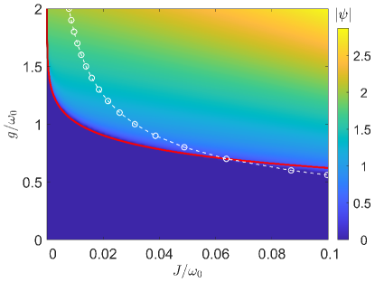
Figure 1: (color online). The steady state phase diagram of the order parameter $|\psi|$ at zero temperature. The red solid line shows the phase boundary described by the analytical solution at Eq. (18), and the white dashed curve with circles shows the boundary based on the LME Fazio_DPT_RH . The other system parameters are given by $\varepsilon=\omega_{0}$, z=3, $\gamma_{q}=\gamma_{c}=10^{-4}\omega_{0}$.  The selected system parameters are consistent with previous works, e.g., $\omega_{0}/2\pi=\varepsilon/2\pi=6$ GHz, $\gamma_{q}/\omega_{0}=\gamma_{c}/\omega_{0}{=}0.2{\times}10^{-4}$ in Ref. dressedME ; $\omega_{0}/2\pi=4$ GHz, $\varepsilon/2\pi=8$ GHz, $\gamma_{q}/\omega_{0}=\gamma_{c}/\omega_{0}=1.8{\times}10^{-4}$ in Ref. lg2015pra .

We first apply  the DME combined with mean-field theory to numerically investigate the phase diagram of photons of the Rabi-Hubbard model at zero temperature.  By calculating the order parameter $|\psi|$ with Eq. (10), the sharp phase transition of photons from the localization to the delocalization phase is clearly exhibited in Fig.1. The localization phase with vanished order parameter (i.e., $|\psi|=0$) is denoted by the dark blue region, whereas the delocalization phase, characterized as significant excitation of the order parameter, locates at light green and yellow regions. The present phase transition corresponds to the $Z_{2}$ symmetry breaking. As the inter-site photon tunneling strength $J$ increases, the critical on-site qubit-photon coupling strength $g_{c}$ separating the delocalization and localization phases decreases gradually.  In particular, as $g_{c}$ approaches $\infty$, it is found that the corresponding $J_{c}{\rightarrow}0$. We also study the phase boundary at finite temperature, e.g., $T=0.05\omega_{0}$ in Fig. 2. The delocalization phase is partially suppressed, particularly in the weak photon tunneling regime, which leads to finite $J_{c}$ for $g_{c}{\rightarrow}\infty$. Hence,  the thermal noise favors the localization phase of photons.

These numerical results are qualitatively consistent with the previous ones observed in the QPT of light at both the steady state QPT_RH and the ground state Fazio_DPT_RH , where the competition between the inter-site photon tunneling and the on-site qubit-photon coupling are also considered. In the next subsection, we analytically explain the global boundary through the order parameter of photons.

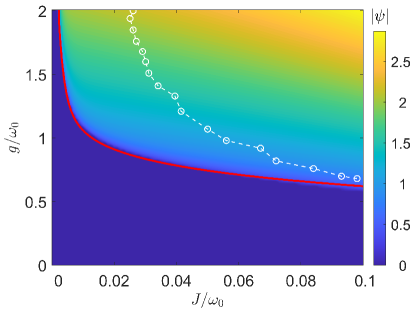
Figure 2: (color online). The steady state phase diagram of the order parameter $|\psi|$ at finite temperature, $T_{q}=T_{c}=0.05\omega_{0}$. The red solid line shows the phase boundary described by the analytical solution at Eq. (21), and the white dashed curve with circles shows the boundary based on the LME numerically. The other system parameters are the same as those in Fig. 1.

III.2 Analytical solution of quantum phase transition

Since the phase boundary located by numerical calculation in Fig. 1 is just in the deep-strong coupling regime where the analytical adiabatic approximation can be applicable Irish2005prb , we may also derive an analytical solution of the order parameter $|\psi|$ at steady state in the critical regime. Specifically, at steady state ($d\rho_{ij}^{ss}/dt=0$) we obtain the  following relations from Eqs. (12a)-(12b)

$$\text{Im}\{\rho^{ss}_{10}\}= \Gamma(\Delta)[n_{\text{B}}(\Delta)+1/2]\text{Re}\{\rho^{ss}_{10}\}/\Delta,~{}$$ (15a)

$$1-2\rho^{ss}_{00}= ({\Gamma^{2}(\Delta)[n_{\text{B}}(\Delta)+1/2]^{2}}/{\Delta}+\Delta)\text{Re}\{\rho^{ss}_{10}\}/\beta_{\psi}~{}.$$ (15b)

In the zero temperature limit, combining Eq. (12b) with Eqs.  (15a) and (15b), the order parameter is obtained as

$$~{}|\psi|\approx\frac{\omega_{0}}{2\sqrt{2}gzJ}\sqrt{\frac{4g^{2}zJ\Delta}{\omega_{0}^{2}}-\Delta^{2}-\frac{\Gamma^{2}(\Delta)}{4}}.$$ (16)

Moreover, from Eq. (16) it is explicitly shown that the emergence of the nonzero order parameter is bounded by the inequality

$$~{}\frac{4g^{2}zJ\Delta}{\omega_{0}^{2}}{\geq}\Delta^{2}+\frac{\Gamma^{2}(\Delta)}{4}.$$ (17)

Such inequality has pronounced consequence on the phase-transition boundary in Fig. 1. Then, we analyze the boundary of QPT of photons from the analytical perspective.

In one previous study of the dissipative Rabi-Hubbard lattice Fazio_DPT_RH , Schiró et al. applied the LME to approximately quantify the phase boundary with the critical tunneling strength at zero temperature $J_{\text{crit}}{\approx}[{\gamma_{c}^{2}g^{2}}/{\omega_{0}^{3}}+{\omega_{0}^{3}}/{16g^{2}}]/d$, with $d$ being the dimensional number, which is also reproduced by the white dashed curve with circles in Fig. 1. In the photon-tunneling regime, $J_{\text{crit}}>0.06\omega_{0}$, their result agrees with the numerical counterpart. However, for the strong qubit-photon coupling, one can note that $J_{\text{crit}}$ has a finite minimal value in Ref. Fazio_DPT_RH , i.e., $\gamma_{c}/2d$. This result is inconsistent with the present numerical result in Fig. 1 and those observed in the Rabi-Hubbard model in absence of the quantum dissipation QPT_RH , in which $J_{\text{crit}}{\propto}\Delta$ vanishes with the increase of $g$.

Here, considering the inequality  (17) with $\Delta$ and $\Gamma(\Delta)$ specified by Eqs. (13) and (14), we obtain the critical tunneling strength as

$$~{}zJ_{c}=\frac{\omega_{0}^{2}\Delta}{4g^{2}}\left[1+\Big{(}\frac{2g^{2}\gamma_{c}}{\omega_{0}^{3}}+\frac{\gamma_{q}}{2\varepsilon}\Big{)}^{2}\right].$$ (18)

It is found that in the absence of quantum dissipation, i.e., $\gamma_{q(c)}=0$, $J_{c}$ is naturally reduced to ${\omega_{0}^{2}\Delta}/{(4zg^{2})}$, which is quite compatible with the result in Ref. QPT_RH . While by tuning on the dissipation, the critical tunneling strength is shifted up by the cooperative contribution of the dissipation strengths, i.e., $\gamma_{q}$ and $\gamma_{c}$. However, as the qubit-photon coupling becomes deep strong, $J_{c}$ again approaches zero, as indicated by the red curve in Fig. 1. We immediately note that this result at Eq. (18) is different from that based on the LME in Ref. Fazio_DPT_RH in the strong qubit-photon interaction regime.

Physically,  the DME captures the microscopic transitions from the eigenstate $|\phi_{1}^{\text{Rabi}}{\rangle}$ to $|\phi_{0}^{\text{Rabi}}{\rangle}$, which is characterized as the rate $\Gamma(\Delta)$  (14). Hence, the dynamical transition in  the DME generally relies on the energy gap, e.g., by selecting Ohmic (in this work) or super-Ohmic types of thermal baths, which leads to the result that $J_{c}{\rightarrow}0$ as $g_{c}{\rightarrow}\infty$. In contrast, LME phenomenologically treats $\Gamma(\Delta)$ independent of the energy gap, which generally overestimates the dissipative processes at strong qubit-photon coupling. Therefore, we believe that  the DME may generally improve the boundary from the microscopic view.

We also analyze the phase boundary at finite temperatures. From Eqs. (12b), (15a), and (15b), the order parameter $|\psi|$ can be obtained as

$$|\psi| \approx \sqrt{\frac{4g^{2}zJ\Delta}{(2n_{\text{B}}(\Delta)+1)\omega_{0}^{2}}-\Delta^{2}-\frac{\left[(2n_{\text{B}}(\Delta)+1)\Gamma(\Delta)\right]^{2}}{4}}$$ (19)

$${\times}\frac{\omega_{0}}{2\sqrt{2}gzJ}.$$

Meanwhile, the nonzero order parameter is bounded by the inequality

$$~{}\frac{4g^{2}zJ\Delta}{[2n_{\text{B}}(\Delta)+1]\omega_{0}^{2}}{\geq}\Delta^{2}+\frac{[2n_{\text{B}}(\Delta)+1]^{2}\Gamma^{2}(\Delta)}{4}.$$ (20)

Hence, we may predict the critical tunneling strength at finite temperature as

$$~{}zJ_{c} = {\frac{\omega_{0}^{2}\Delta}{4g^{2}}}[2n_{\text{B}}(\Delta)+1]\{1+[2n_{\text{B}}(\Delta)+1]^{2}$$ (21)

$$\times({2g^{2}\gamma_{c}}/{\omega_{0}^{3}}+{\gamma_{q}}/{2\varepsilon})^{2}\},$$

which is naturally reduced to Eq. (18) as $T$ approaches aero. From Fig. 2 it is found that $J_{c}$ (the red solid line) based on  the DME agrees well with the numerical result in a wide qubit-photon coupling regime. Hence, the analytical expression of critical tunneling strength at Eq. (21) may be helpful to deepen the understanding of the finite temperature phase transitions of photons. However, we should admit that this analytical result deviates from the numerical one at extremely strong qubit-photon coupling limit ($\Delta{\approx}0$), where $J_{c}{\propto}g^{2}\exp(4g^{2}/\omega_{0}^{2})$ is significantly enhanced as $n_{\text{B}}{\approx}k_{B}T/\Delta$. Moreover, the two-dressed-state approximation may break down at high-temperature regime, and more dressed states should be considered like in the numerical analysis.

IV Conclusion

In this paper, we study the QPT of light in the Rabi-Hubbard lattice with local dissipation under the framework of the mean-field theory and the quantum dressed master equation. The steady-state phase diagram of photons are numerically calculated, which clearly classifies the localization and delocalization phases. We then analytically obtain an approximate expression of the order parameter in the low temperature and deep-strong qubit-photon coupling regime, where the mean-field Rabi model is reduced to the effective nearly degenerate two-dressed-state system. We further analyze the boundary between two difference phases at zero temperature, which is characterized as the critical tunneling strength.  The expression of the critical tunneling strength in the absence of the quantum dissipation can be naturally reduced to the previous ones, see, e.g., Ref. Fazio_DPT_RH . While by tuning on the quantum dissipation, which is characterized by representative thermal baths, e.g., Ohmic or super-Ohmic type, it is found that the critical tunneling strength approaches zero as the qubit-photon coupling strength becomes deep-strong. This result is generally distinct from the previous work based on  the LME, which in contrast has finite minimal critical tunneling strength. We also predict the critical tunneling strength at finite temperatures, which may be helpful to study the phase transition of light at thermal equilibrium. In the future, it should be interesting to explore the steady-state phase diagram of photons in the Rabi-Hubbard model beyond the simple mean-field framework, e.g., based on the cluster mean-field theory jsjin2016prx and linked-cluster expansion approach ab2018prb .

V Acknowledgements

T. Y and Q.-H.C. are supported by the National Science Foundation of China under Grant No. 11834005, the National Key Research and Development Program of China under Grant No. 2017YFA0303002. C.W. acknowledges the National Natural Science Foundation of China under Grant No. 11704093 and the Opening Project of Shanghai Key Laboratory of Special Artificial Microstructure Materials and Technology.

References

- (1) M. O. Scully and M. S. Zubairy, Quantum Optics (Cambridge University Press, London, 1997).
- (2) S. Barik, A. Karasahin, C. Flower, T. Cai, H. Miyake, W. DeGottardi, M. Hafezi, and E. Waks, Science 359, 666 (2018).
- (3) L. Lu, J. D. Joannopoulos, and M. Soljačić, Nat. Photonics 8, 821 (2014).
- (4) K. Le Hur, L. Henriet, A. Petrescu, K. Plekhanov, G. Roux, and M. Schiró, C. R. Phys. 17, 808 (2016).
- (5) T. Ozawa, H. M. Price, A. Amo, N. goldman, M. Hafezi, L. Lu, M. C. Rechtsman, D. Schuster, J. Simon, O. Zilberberg, and L. Carusotoo, Rev. Mod. Phys. 91, 015006 (2019).
- (6) R. F. Ribeiro, L. A. Martínez-Martínez, M. Du, J. C. G. Angulo, and J. Y. Zhou, Chem. Sci. 9, 6325 (2018).
- (7) J. Y. Zhou and V. M. Menon, Proc. Natl. Acad. Sci. U. S. A. 116, 5214 (2019).
- (8) T. Niemczyk, F. Deppe, H. Huebl, E. P. Menzel, F. Hocke, M. J. Schwarz, J. J. Garcia-Ripoll, D. Zueco, T. Hümmer, E. Solano, A. Marx and R. Gross, Nat. Phys. 6, 772 (2010).
- (9) P. Forn-Díaz, J. Lisenfeld, D. Marcos, J. J. GarcDía-Ripoll, E. Solano, C. J. P. M. Harmans, and J. E. Mooij, Phys. Rev. Lett. 105, 237001 (2010).
- (10) J. S. Pedernales, I. Lizuain, S. Felicetti, G. Romero, L.Lamata, and E. Solano, Sci. Rep. 5, 15472 (2015).
- (11) S. Felicetti, E. Rico, C. Sabin, T. Ockenfels, J. Koch, M. Leder, C. Grossert, M. Weitz, and E. Solano, Phys. Rev. A 95, 013827 (2017).
- (12) I. I. Rabi, Phys. Rev. 49, 324 (1936).
- (13) E. T. Jaynes and F. W. Cummings, Proc. IEEE 51, 89 (1963).
- (14) F. Yoshihara, T. Fuse, S. Ashhab, K. Kakuyanagi, S. Saito, and K. Semba, Nat. Phys. 13, 44 (2017).
- (15) F. Beaudoin, J. M. Gambetta, and A. Blais, Phys. Rev. A 84, 043832 (2011).
- (16) D. Braak, Phys. Rev. Lett. 107, 100401 (2011).
- (17) Q.-H. Chen, C. Wang, S. He, T. Liu, and K. L. Wang, Phys. Rev. A 86, 023822 (2012).
- (18) D. Braak, Q. H. Chen, M. Batchelor, and E. Solano, J. Phys.A: Math. Theor. 49, 300301 (2016).
- (19) P. Forn-Díaz, L. Lamata, E. Rico, J. Kono, and E. Solano, Rev. Mod. Phys. 91, 025005 (2019); A. F. Kockum, A. Miranowicz, S. De Liberato, S. Savasta, and F. Nori, Nat. Rev. Phys. 1, 19 (2019).
- (20) N. S. Mueller, Y. Okamura, B. G. M. Vieira, S. Juergensen, H. Lange, E. B. Barros, F. Schulz, S. Reich, Nature (London) 583, 780 (2020).
- (21) P. Kirton, M. M. Roses, J. Keeling and E. G. Dalla Torre, Adv. Quantum Technol. 2 1800043 (2019).
- (22) M. J. Hwang, R. Puebla, and M. B. Plenio, Phys. Rev. Lett. 115, 180404 (2015).
- (23) M. X. Liu, S. Chesi, Z. J. Ying, X. S. Chen, H. G. Luo, and H. Q. Lin, Phys. Rev. Lett. 119, 220601 (2017).
- (24) A. D. Greentree, C. Tahan, J. H. Cole, and L. C. Hollenberg, Nat. Phys. 2, 856 (2006).
- (25) M. Hartmann, F. Brandao, and M. Plenio, Nat. Phys. 2, 849 (2006).
- (26) S. C. Lei and R. K. Lee, Phys. Rev. A 77, 033827 (2008).
- (27) J. Koch and K. Le Hur, Phys. Rev. A 80, 023811 (2009).
- (28) S. Schimidt and G. Blatter, Phys. Rev. Lett. 103, 086403 (2009).
- (29) C. Nietner and A. Pelster, Phys. Rev. A 85, 043831 (2012).
- (30) J. B. You, W. Yang, Z. Y. Xu, A. Chan, and C. Oh, Phys. Rev. B 90, 195112 (2014).
- (31) B. Bujnowski, J. K. Corso, A. L. C. Hayward, J. H. Cole, and A. M. Martin Phys. Rev. A 90, 043801 (2014).
- (32) A. Hayward and A. Martin, Phys. Rev. A 93, 023828 (2016).
- (33) H. Zheng and Y. Takada, Phys. Rev. A 84, 043819 (2011).
- (34) M. Schiró, M. Bordyuh, B. Öztop and H. E. Türeci, Phys. Rev. Lett. 109, 053601 (2012).
- (35) M. Schiró, M. Bordyuh, B. Öztop, and H. E. Türeci, J. Phys. B: At., Mol. Opt. Phys. 46, 224012 (2013).
- (36) Y. C. Lu and C. Wang, Quantum Inf. Process. 15 4347 (2016).
- (37) U. Weiss, Quantum dissipative dynamics (World Scientific, Singapore, 2012).
- (38) R. C. Wu, L. Tan, W. X. Zhang, and W. M. Liu, Phys. Rev. A 96, 033633 (2017).
- (39) M. Schiró , C. Joshi, M. Bordyuh, R. Fazio, J. Keeling, and H. E. Türeci, Phys. Rev. Lett. 116, 143603 (2016).
- (40) A. Settineri, V. Macrí, A. Ridolfo, O. Di Stefano, A. F. Kockum, F. Nori and S. Savasta, Phys. Rev. A 98, 053834 (2018).
- (41) A. Le Boité, Adv. Quantum Technol., 3, 1900140 (2020).
- (42) L. Garziano, R. Stassi, V. Macrí, A. F. Kockum, S. Savasta, and F. Nori, Phys. Rev. A 92, 063830 (2015).
- (43) A. Ridolfo, M. Leib, S. Savasta, and M. J. Hartmann, Phys. Rev. Lett. 109, 193602 (2012).
- (44) A. Ridolfo, S. Savasta, and M. J. Hartmann, Phys. Rev. Lett. 110, 163601 (2013).
- (45) A. Le Boité, M. J. Hwang, H. C. Nha, and M. B. Plenio, Phys. Rev. A 94, 033827 (2016).
- (46) A. Le Boité, M. J. Hwang, and M. B. Plenio, Phys. Rev. A 95, 023829 (2017).
- (47) D. van Oosten, P. van der Straten, and H. R. Krishnamurthy, Phys. Rev. A 63, 053601 (2001).
- (48) D. van Oosten, P. van der Straten, and H. R. Krishnamurthy, Phys. Rev. A 67, 033606 (2003).
- (49) A. A. Houck, H. E. Türeci, and J. Koch, Nat. Phys. 8, 292 (2012).
- (50) I. Carusotto and C. Ciuti, Rev. Mod. Phys. 85, 299 (2013).
- (51) M. Fitzpatrick, N. M. Sundaresan, A. C. Y. Li, J. Koch, and A. A. Houck, Phys. Rev. X 7, 011016 (2017).
- (52) A. J. Kollár, M. Fitzpatrick, and A. A. Houck, Nature (London) 571, 45 (2019).
- (53) I. Carusotto, A. A. Houck, A. J. Kollár, P. Roushan, D. I. Schuster, and J. Simon, Nat. Phys. 16, 268 (2020).
- (54) E. K. Irish, J. Gea-Banacloche, I. Martin, and K. C. Schwab, Phys. Rev. B 72, 195410(2005).
- (55) J. S. Jin, A. Biella, O. Viyuela, L. Mazza, J. Keeling, R. Fazio, and D. Rossini, Phys. Rev. X 6, 031011 (2016).
- (56) A. Biella, J. S. Jin, O. Viyuela, C. Ciuti, R. Fazio, and D. Rossini, Phys. Rev. B 97, 035103 (2018).