Graph coarsening: From scientific computing to machine learning

Abstract

The general method of graph coarsening or graph reduction has been a remarkably useful and ubiquitous tool in scientific computing and it is now just starting to have a similar impact in machine learning. The goal of this paper is to take a broad look into coarsening techniques that have been successfully deployed in scientific computing and see how similar principles are finding their way in more recent applications related to machine learning. In scientific computing, coarsening plays a central role in algebraic multigrid methods as well as the related class of multilevel incomplete LU factorizations. In machine learning, graph coarsening goes under various names, e.g., graph downsampling or graph reduction. Its goal in most cases is to replace some original graph by one which has fewer nodes, but whose structure and characteristics are similar to those of the original graph. As will be seen, a common strategy in these methods is to rely on spectral properties to define the coarse graph.

05C50, 05C85, 65F50, 68T09.

1 Introduction

The idea of ‘coarsening,’ i.e., exploiting a smaller set in place of a larger or ‘finer’ set has had numerous uses across many disciplines of science and engineering. The term ‘coarsening’ employed here is prevalent in scientific computing, where it refers to the usage of coarse meshes to solve a given problem by, e.g., multigrid (MG) or algebraic multigrid (AMG) methods. On the other hand, the terms ‘graph downsampling,’ ‘graph reduction,’ ‘hierarchical methods,’ and ‘pooling’ are common in machine learning. Similarly, the related idea of clustering is an important tool in data-based applications. Here, the analogous term employed in scientific computing is ‘partitioning.’ These notions—graph partitioning, clustering, coarsening—are strongly inter-related. It is possible to use partitioning for the task of clustering data, by first building a graph that models the data which we then partition. Also, coarsening plays an important role in developing effective graph partitioning methods. Further, note that it is possible to partition a graph by just finding some clustering of the nodes, using a method from data sciences such as the K-means algorithm.

In scientific computing, the best known instance of coarsening techniques is in MG and AMG methods [57, 100, 115, 28]. Classical MG methods started with the independent works of Bakhvalov [10] and Brandt [24]. The important discovery revealed by these pioneering articles is that relaxation methods for solving linear systems tend to stall after a few steps, because they have difficulty in reducing high-frequency components of the error. Because the eigenvectors associated with a coarser mesh are direct restrictions of those on the fine mesh, the idea is to project the problem into an ‘equivalent’ problem on the coarse mesh for error correction and then interpolate the solution back into the fine level. This basic 2-level scheme can be extended to a multilevel one in a variety of ways. MG does not use graph coarsening specifically because it relies on a mesh and it is more natural to define a coarse mesh using processes obtained from the discretization of the physical domain. On the other hand, AMG aims at general problems that do not necessarily have a mesh associated with them. For AMG, the graph representation of the problem at a certain level is explicitly ‘coarsened’ by using various mechanisms [100, 28, 101]. Since these mechanisms are geared toward a certain class of problems, essentially originating from Poisson-like partial differential equations, researchers later sought to extend AMG ideas in order to define algebraic techniques based on incomplete LU (ILU) factorizations [11, 89, 117, 6, 4, 5, 7, 9, 8, 23].

One can say that the idea of coarsening a graph in data-related applications started with the 1939 article of Kron [71], whose aim was to downsample electrical networks. Kron used his deep intuition to define coarsening techniques that rely on Schur complements, with the goal of obtaining sparse graphs. The justifications for the proposed technique were based on intuition rooted on knowledge about electrical networks. The related technique, widely known as Kron reduction, was revived by Dörfler and Bullo [46] who provided a more rigorous theoretical foundation. Later Shuman et al. [108] extended the Kron reduction into a multilevel framework. In parallel with this line of work, a number of authors developed techniques that bypassed the need to form or approximate the Schur complement relying instead on node aggregation and matching [61, 63, 73, 35, 114, 95, 94, 105].

Applications of graph coarsening in machine learning generally fall in two categories. First, coarsening is instrumental in graph embeddings. When dealing with learning tasks on graphs, it is very convenient to represent a node with a vector in $\mathbb{R}^{d}$ where $d$ is small. The mapping from a node to the representing vector is termed node (or vertex) embedding and finding such embeddings tends to be costly. Hence, the idea is to coarsen the graph first, perform some embedding at the coarse level, and then refine-propagate the embedding back to the upper level; see [35, 73, 42, 93] for examples of such techniques. The second category of applications is when invoking pooling on graphs, in the context of graph neural networks (GNNs) [125, 126, 76]. However, in the latest development of GNNs, coarsening is not performed on the given graph at the outset. Instead, coarsening is part of the neural network and it is learned from the data. Another class of applications of coarsening is that of graph filtering, as illustrated by the articles [108, 109].

The goal of this paper is to show how the idea of coarsening has been exploited in scientific computing and how it is now emerging in machine learning. While the problems under consideration in scientific computing are fundamentally different from those of machine learning, the basic ingredients used in both methods are striking by their similarity. The paper starts with a discussion of graph coarsening in scientific computing (Section 2), followed by a section on graph coarsening in machine learning (Section 3). We also present some newly developed coarsening methods and results, in the context of machine learning, in Sections 4–5.

1.1 Notation and preliminaries

We denote by $G=(V,E)$ a graph with $n$ nodes and $m$ edges, where $V$ is the node set and $E$ is the edge set. The weights of the edges of $G$ are stored in a matrix $A$, so $a_{ij}$ is the weight of the edge $(i,j)\in E$. In most cases we will assume that the graph is undirected. We sometimes use $G=(V,E,A)$ to denote the graph, when $A$ is emphasized.

The sum of row $i$ of $A$ is called the degree of node $i$ and the diagonal matrix of the degrees is called the degree matrix:

(1) $$d_{i}=\sum_{j=1}^{n}a_{ij};\quad D=\mbox{diag}(d_{i}).$$

With this notation, the graph Laplacian matrix $L$ is defined as:

(2) $$L=D-A.$$

This definition implies that $L\mathbf{1}=0$ where $\mathbf{1}$ is the vector of all ones; i.e., $\mathbf{1}$ is an eigenvector associated with the eigenvalue zero. In the simplest case, each weight $a_{ij}$ is either zero (not adjacent) or one (adjacent). A simple, yet very useful, property of graph Laplacians is that for any vector $x$, we have the relation

(3) $$x^{T}Lx=\sum_{ij}a_{ij}|x_{i}-x_{j}|^{2}\ .$$

The normalized Laplacian is defined as follows:

(4) $$\widehat{L}=D^{-1/2}LD^{-1/2}=I-D^{-1/2}AD^{-1/2}\ .$$

Note that the diagonal entries of $\widehat{L}$ are all ones. The matrix is again singular and has the null vector $D^{1/2}\mathbf{1}$.

We will also make use of the incidence matrix denoted by $B\in\mathbb{R}^{n\times m}$. A column $b_{e}$ of $B$ represents an edge $e\in E$ between nodes $i$ and $j$ with weight $a_{ij}$, and its $k$-th entry is defined as follows:

(5) $$b_{e}(k)=\begin{cases}+\sqrt{a_{ij}},&k=i,\\ -\sqrt{a_{ij}},&k=j,\\ 0,&\text{otherwise}.\end{cases}$$

Note that the two nonzero values of $b_{e}(k)$ have opposite signs, but we have a choice regarding which of $i$ and $j$ is assigned the negative sign. Unless otherwise specified, we simply assign the negative sign to the smaller of $i$ and $j$. As is well-known, the graph Laplacian can be defined from the incidence matrix through the relation $L=BB^{T}$.

1.2 Terminology and notation specific to machine learning

In data-related applications, graph nodes are often equipped with feature vectors and labels. We use an $n\times d$ matrix $X$ to denote the feature matrix, whose $i$-th row is the feature vector of node $i$. We use an $n\times c$ matrix $Y$ to denote the label matrix, where $c$ is the number of categories. When a node $i$ belongs to category $j$, $Y_{ij}=1$ while $Y_{ij^{\prime}}=0$ for all $j^{\prime}\neq j$. Each row of $Y$ is called a ‘one-hot’ vector. When there are only two categories, the $n\times 2$ matrix $Y$ can equivalently be represented by an $n\times 1$ binary vector $y$ in a straightforward manner.

For example, in a transaction graph, where nodes represent account holders and edges denote transactions between accounts, a node may have $d=4$ features: account balance, account active days, number of incoming transactions, and number of outgoing transactions; as well as $c=3$ categories: individual, non-financial institution, and financial institution. A typical task is to predict the account category given the features.

The feature matrix $X$ provides complementary information to a graph $G=(V,E,A)$ that captures relations between data items. One should not confuse the feature matrix with a data matrix, which by convention clashes with the notation $X$. Let us use $Z$ instead to denote a data matrix, whose $i$-th row is denoted by $z_{i}$. One may construct the graph $G$ from $Z$. For example, in a $k$-nearest neighbors ($k$NN) graph, there is an edge from node $i$ to node $j$ if and only if $j$ is an index of the element among the $k$ smallest elements of $\{r_{ij}=\|z_{j}-z_{i}\|\mid j\neq i\}$. One may even define the weighted adjacency matrix $A$ as $a_{ij}=e^{-r_{ij}}$ when there is an edge $(i,j)$ and $a_{ij}=0$ otherwise. In this case, the constructed graph is entirely decided by the data matrix $Z$, rather than by holding complementary information to it, as is done with the feature matrix.

2 Graph coarsening in scientific computing

Given a graph $G=(V,E)$, the goal of graph coarsening is to find a smaller graph $G_{c}=(V_{c},E_{c})$ with $n_{c}$ nodes and $m_{c}$ edges, where $n_{c}<n$, which is a good approximation of $G$ in some sense. Specifically, we would like the coarse graph to provide a faithful representation of the structure of the original graph. We denote the adjacency matrix of $G_{c}$ by $A_{c}$ and the graph Laplacian of $G_{c}$ by $L_{c}$.

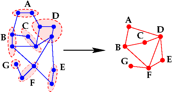
Figure 1: Coarsening a graph.

We will first elaborate on one of the most important scenarios that invoke coarsening (Section 2.1) and then discuss several representative approaches to it (Sections 2.2 to 2.5). Note that in practice, coarsening often proceeds recursively on the resulting graphs; by doing so, we obtain a hierarchy of approximations to the original graph.

2.1 Multilevel methods for linear systems: AMG and multilevel ILU

Graph coarsening strategies are usually invoked when solving linear systems of equations, by multilevel methods such as (A)MG [57, 115, 100] or Schur-based multilevel techniques [37, 104, 89, 79, 78, 11, 7]. In (A)MG, this amounts to selecting a subset of the original (fine) grid, known as the ‘coarse grid.’ In AMG, the selection of coarse nodes is made in a number of different ways. The classical Ruge-Stüben strategy [100] selects coarse nodes based on the number of ‘strong connections’ that a node has. Here, nodes $i$ and $j$ are strongly connected if $a_{ij}$ has a large magnitude relative to other nonzero off-diagonal elements or row $i$. The net effect of this strategy is that each fine node is strongly coupled with the coarse set. In other methods, the strength of connection is defined from the speed with which components of a relaxation scheme for solving the homogeneous system $Au=0$ converge to zero; see [25, 97, 36] and Section 2.4 for additional details. For multilevel Schur-based methods, such as multilevel ILU, the coarsening strategy may correspond to selecting from the adjacency graph of the original matrix, a subset of nodes that form an independent set [104], or a subset of nodes that satisfy good diagonal dominance properties [102] or that limit the growth in the inverse LU factors of the ILU factorization [21, 22].

The coarsening strategy can be expanded into a multilevel framework by repeating the process described above on the graph associated with the nodes in the coarse set. Let $G_{0}$ be the original graph $G$ and let $G_{1},G_{2},\ldots,G_{m}$ be a sequence of coarse graphs such that $G_{\ell}=(V_{\ell},E_{\ell})$ is obtained by coarsening on $G_{\ell-1}$ for $1\leq\ell<m$. Let $A^{(0)}\equiv A$ and $A^{(\ell)}$ be the matrix associated with the $\ell$-th level. The graph $G_{\ell}$ admits a splitting into coarse nodes, $C_{\ell}$, and fine nodes, $F_{\ell}$, so that the linear system at the $\ell$-th level, which consists of the matrix $A^{(\ell)}$ and the right-hand side $f^{(\ell)}$ can be reordered as follows:

(6) $$A^{(\ell)}=\left[\begin{array}[]{cc}A^{(\ell)}_{CC}&A^{(\ell)}_{CF}\\ A^{(\ell)}_{FC}&A^{(\ell)}_{FF}\end{array}\right]\ ,\quad f^{(\ell)}=\begin{bmatrix}f^{(\ell)}_{C}\\ f^{(\ell)}_{F}\end{bmatrix}.$$

Note that it is also possible to list the fine nodes first followed by the coarse nodes; see [89]. The coarser-level graph $G_{\ell+1}$ as well as the new system consisting of the matrix $A^{(\ell+1)}$ and the right-hand side $f^{(\ell+1)}$ at the next level, are constructed from $G_{\ell}$ and $A^{(\ell)}$. These are built in a number of different ways depending on the method under consideration. For the graph, we can for example set two coarse nodes to be adjacent in $G_{\ell+1}$, if their representative children are adjacent in $G_{\ell}$. One common way to do this is to define two coarse nodes to be adjacent in $G_{\ell+1}$ if they are parents of adjacent nodes in $G_{\ell}$. Next we discuss coarsening in the specific context of AMG.

2.1.1 Algebraic multigrid

AMG techniques are all about generalizing the interpolation and restriction operations of standard MG. The coarsening process identifies for each fine node a set of nearest neighbors from the coarse set. Using various arguments on the strength of connection between nodes, AMG expresses a fine node $i$ as a linear combination of a selected number of nearest neighbors that form a set $C_{i}$, see Figure 2. To simplify notation, we consider only one level of coarsening and drop the subscript $\ell$.

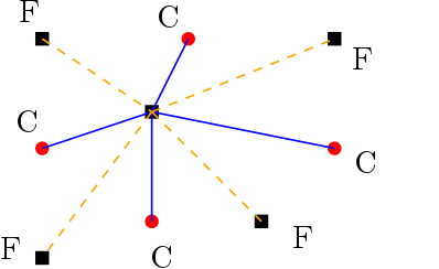
Figure 2: A fine node and its nearest neighbors. Fine nodes are represented by a square and coarse ones by a disk. In the coarsening process the central, fine node is expressed as a combination of its coarse neighbors.

If $C$ is the set of coarse nodes and $F$ is the set of fine nodes, we can define related subspaces $\mathcal{X}_{C}$ and $\mathcal{X}_{F}$ of the original space $\mathcal{X}=\mathbb{R}^{n}$. In fact we can write $\mathcal{X}=\mathcal{X}_{C}\oplus\mathcal{X}_{F}$. Then, given a vector $x$ with components in the coarse space $\mathcal{X}_{C}$, we associate a vector $Px$ in the original space $\mathcal{X}$, whose $i$-th component is defined as follows [103, 13.6.2]:

(7) $$[Px]_{i}=\left\{\begin{array}[]{ll}x_{i}&\mbox{if}\ i\ \in C,\\ \sum_{j\in C_{i}}p_{ij}x_{j}&\mbox{otherwise}.\end{array}\right.$$

The mapping $P$ sends a point of $\mathcal{X}_{C}$ into a point $y=Px$ of $\mathcal{X}$. The value of $y$ at a coarse point, a node in $C$, is the same as its starting value. The value at another node, one in $F$, is defined from interpolated values at a few coarse points. Thus, $P$ is known as the interpolation operator.

The transpose of $P$ represents the restriction, or coarsening mapping. In the context of AMG, it projects a point in $\mathcal{X}$ into a point in $\mathcal{X}_{C}$. Each node in $C$ is a linear combination of nodes of the original graph.

If we now return to the multilevel case where $P_{\ell}$ denotes a corresponding interpolation operator at the $\ell$-th level, then AMG defines the linear system at the next level using Galerkin projection, where the matrix and right-hand side are, respectively,

(8) $$A^{(\ell+1)}=P_{\ell}^{T}A^{(\ell)}P_{\ell},\quad f^{(\ell+1)}=P_{\ell}^{T}f^{(\ell)}\ .$$

Recall that we started with the original system $A^{(0)}x=f^{(0)}$, which corresponds to $\ell=0$. AMG methods rely on a wide variety of iterative procedures that consist of exploiting different levels for building an approximate solution. It is important to note here that the whole AMG scheme depends entirely on defining a sequence of interpolation operators $P_{\ell}$ for $\ell=0,1,\ldots$ Once the $P_{\ell}$’s are defined, one can design various ‘cycles’ in which the process goes back and forth from the finest level to the coarsest one in an iterative procedure.

When defining the interpolation operator $P_{\ell}$, there are two possible extremes worth noting, even though these extremes are not used in AMG in practice. On the one end, we find the trivial interpolation in which the $p_{ij}$’s in equation (7) are all set to zero. In this case, referring to (6), $A^{(\ell+1)}$ is simply $A^{(\ell+1)}=A_{CC}^{(\ell)}$.

The other extreme is the perfect interpolation case which yields the Schur complement system. Here, the interpolation operator is

$$P_{\ell}=\begin{bmatrix}-[A_{CC}^{(\ell)}]^{-1}A_{CF}^{(\ell)}\\ I\end{bmatrix}.$$

The right reduced matrix $A^{(\ell)}P_{\ell}$ involves the Schur complement matrix associated with the coarse block:

$$A^{(\ell)}P_{\ell}=\begin{bmatrix}O\\ S_{\ell}\end{bmatrix}\quad\mbox{where}\quad S_{\ell}=A_{FF}^{(\ell)}-A_{FC}^{(\ell)}[A_{CC}^{(\ell)}]^{-1}A_{CF}^{(\ell)}.$$

Then clearly,

$$A^{(\ell+1)}=P_{\ell}^{T}A^{(\ell)}P_{\ell}=S_{\ell}.$$

Since this is the exact Schur complement, if we were to solve the related linear system, we could recover the whole solution of the original system by substitution. This approach is costly but there are practical alternatives discussed in the literature [21, 117, 11, 81] that are based on Schur complements. However, it is worth pointing out that, viewed from this angle, the goal of all AMG methods is essentially to find inexpensive approximations to the Schur complement system.

2.1.2 Multilevel ILU preconditioners based on coarsening

The issue of finding a good ordering for ILU generated a great deal of research interest in the past; see, e.g., [18, 19, 17, 26, 39, 45, 40, 27, 102, 38]. A class of techniques presented in [89] consisted of preprocessing the linear system with an ordering based on coarsening. Thus, for a one-level ordering the matrix is ordered as shown in (6). Then in a second level coarsening, $A_{22}^{(0)}$ is in turn reordered and we end up with a matrix like:

$$\left[\begin{array}[]{c|c}A_{11}^{(0)}&A_{12}^{(0)}\\ \hline\cr A_{21}^{(0)}&\begin{array}[]{c|c}A_{11}^{(1)}&A_{12}^{(1)}\\ \hline\cr A_{21}^{(1)}&A_{22}^{(1)}\end{array}\end{array}\right].$$

This is repeated with $A_{22}^{(1)}$ and further down for a few levels. Then the idea is simply to perform an ILU factorization of the resulting reordered system. Next, we describe a method based on this general approach.

The first ingredient of the method is to define a weight $w_{ij}$ for each nonzero pair $(i,j)$. This will set an order in which to visit the edges of the graph. The strategies described next are ‘static’ in that given a certain matrix $A$ (one of the $A^{(\ell)}$’s), these weights are precomputed, in contrast with dynamic ones used in, e.g., [104, 77, 102]. If $n_{i}$ is the number of nonzero entries of row $i$ and $m_{j}$ is the number of nonzero entries of column $j$, we define the weights as follows:

(9) $$w_{ij} = \min\left\{\frac{|a_{ij}|}{\delta_{r}(i)}\ ,\ \frac{|a_{ij}|}{\delta_{c}(j)}\right\}\ \mbox{where:}$$

(10) $$\delta_{r}(i) = \ \frac{\|A_{i,:}\|_{1}}{n_{i}}\quad\mbox{and}\quad\delta_{c}(j)\ =\ \frac{\|A_{:,j}\|_{1}}{m_{j}}$$

where matlab notation is exploited and $\|\cdot\|_{1}$ is the usual 1-norm. The two terms in the brackets of (9) represent the importance of $|a_{ij}|$ relative to the other elements in the same row and column, respectively. If our goal is to put large entries in the (1,2) block of the matrix when it is permuted (block $A_{CF}^{(\ell)}$ in (6)), then we need to traverse the graph starting from the largest to smallest $w_{ij}$.

The above defines an order in which to visit edges. Next, each time an edge $(i,j)$ is visited we need to determine which one of $i$ and $j$ will be selected as a coarse node. This requires a ‘preference’ measure, or weight, for each node. When $a_{kk}\neq 0$ we define the impact of ‘pivot’ $k$ as the average potential fill-in created when eliminating unknown $k$. In the formula $a_{ij}=a_{ij}-a_{ik}\times a_{kj}/a_{kk}$ employed in the $k$-th step of Gaussian elimination, the term $-a_{ik}\times a_{kj}/a_{kk}$ is a potential fill-in. This is a very crude approximation because it assumes that the entries have not changed. We define the ‘impact’ of the diagonal entry $k$ as the inverse of the quantity:

(11) $$\sigma_{k}=\frac{|a_{kk}|}{\delta_{r}(k)\delta_{c}(k)}\ .$$

When visiting edge $(k,l)$, we add $k$ to the coarse set if $\sigma_{k}>\sigma_{l}$ and $l$ otherwise.

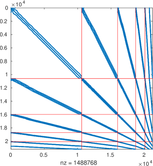
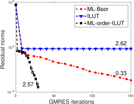
Figure 3: Left: The matrix Raefsky3 after the reordering obtained from four levels of coarsening. Right: Performance of various coarsening based preconditioners for solving a linear system with the matrix.

Here, we show an example on the matrix ‘Raefsky3’, which is of size 21,200 and has 1,488,768 nonzero elements. It comes from a fluid structure interaction turbulence problem and can be obtained from the suite-sparse collection. Figure 3 (left) shows the pattern of the reordered matrix according to the coarsening strategy described above, using four levels of coarsening. The original matrix is not shown but, as expected, its pattern is very similar to that of the (1,1) block of the reordered matrix, and has roughly twice the size.

For this particular matrix, standard ILU-based strategies perform poorly. Using matlab, we applied GMRES(50) to the system, preconditioned with ILU (‘crout’ version) with a drop tolerance of 0.01. The resulting iterates stagnate as indicated by the top curve in the right side of Figure 3. The number 2.62 is the ‘fill-factor,’ which is the ratio of the number of nonzero elements of the LU factors over the the number of nonzero elements of the original matrix. When comparing preconditioners of this type, we strive to ensure that these fill-factors are about the same for the preconditioners being compared. Next we perform an ILU factorization (‘crout’ version again) on the reordered system using the coarsening described above. In order to achieve a fill-factor similar to that of the standard factorization we lowered the drop-tolerance to 0.0008. The new method converged in 29 iterations with a fill factor of 2.57. We also tested a more traditional preconditioner based on block Gauss-Seidel, exploiting the block structure shown on the left side of Figure 3. Each block Gauss-Seidel step requires solving a system with the diagonal blocks of the reordered matrix. These systems are approximately solved using a simple ILU(0) (‘nofill’) factorization. Note that the fill-factor here is very low (0.33). Each preconditioning step consists of 10 Gauss-Seidel iterations. As is shown, this also converges, although more slowly.

2.2 Coarsening approach: Pairwise aggregation

The broad class of ‘pairwise aggregation’ techniques, e.g., [119, 118, 84, 88, 37, 115], is a strategy that seeks to simply coalesce two adjacent nodes in a graph into a single node, based on some measure of nearness or similarity. The technique is based on edge collapsing [62], which is a well known method in the multilevel graph partitioning literature. In this method, the collapsing edges are usually selected using the maximal matching method. A matching of a graph $G=\left(V,E\right)$ is a set of edges $\widetilde{E}$, $\widetilde{E}\subseteq E$, such that no two edges in $\widetilde{E}$ have a node in common. A maximal matching is a matching that cannot be augmented by additional edges to obtain a larger matching in the sense of inclusion. Coarsening schemes based on edge matching have been in use in the AMG literature for decades [100]. For each node $i$, a coarsening algorithm starts from building a set $S_{i}$ of nodes that are ‘strongly connected’ to $i$ by using some measure of connection strength. The graph nodes are traversed in a certain order of preference and the next unmarked node in this order, say $j$, is selected as a coarse node. The priority measure of the traversal is updated after each insertion of a coarse node. There are a number of ways to find a maximal matching for coarsening a graph.

The heavy-edge matching (HEM) approach, e.g., [66], is a greedy matching algorithm that works with the weight matrix $A$ of the graph. It simply matches a node $i$ with its largest off-diagonal neighbor $j_{max}$; i.e., we have $|a_{ij_{max}}|=\max_{j\in adj(i),j\neq i}|a_{ij}|$, where $adj(i)$ denotes the adjacency (or nearest-neighbor) set of node $i$. When selecting the largest neighboring entry, ties are broken arbitrarily. If $j_{max}$ is already matched with some node $k\neq i$ seen before, i.e., $p(k)=j_{max}$, then node $i$ is left unmatched and considered as a singleton. Otherwise, we match $i$ with $j$ and the result is $p(i)=j_{max}$.

Algorithm 1 Heavy Edge Matching (HEM)

1:Input: Weighted graph $G=(V,E,A)$

2:Output: Coarse nodes; $Prnt$ list

3:Init: $Prnt(i)=0$ $\forall i\in V$; $new=0$

4:for $\max$ to $\min$ edge $(i,j)$ do

5:     if $Prnt(i)==0$, $Prnt(j)==0$ then

6:         $new=new+1$

7:         $Prnt(i)=Prnt(j)=new$

8:     end if

9:end for

10:for Node $v$ with $Prnt(v)==0$ do

11:     if $v$ has no neighbor then

12:         $new=new+1$; $Prnt(v)=new$

13:     else

14:         $Prnt(v)=Prnt(j)$ where $j=\mbox{argmax}_{i}(a_{iv})$

15:     end if

16:end for

A version of HEM is shown in Algorithm 1, modified from [89]. The algorithm proceeds by exploiting a greedy approach. It scans all edges $(i,j)$ in decreasing value of their weight $a_{ij}$. If neither $i$ nor $j$ has defined parents, it creates a new coarse node labeled $new$ and sets the parents of $i$ and $j$ to be $new$. After the loop is completed, there will be singletons; i.e., nodes that have not been assigned a parent in the loop. As shown in lines 10–16, a ‘singleton’ node is either added as a coarse node, if it is disconnected (‘real singleton’), or it is lumped as a child of an already generated coarse node (‘left-over singleton’). Figure 4 gives an illustration of this step.

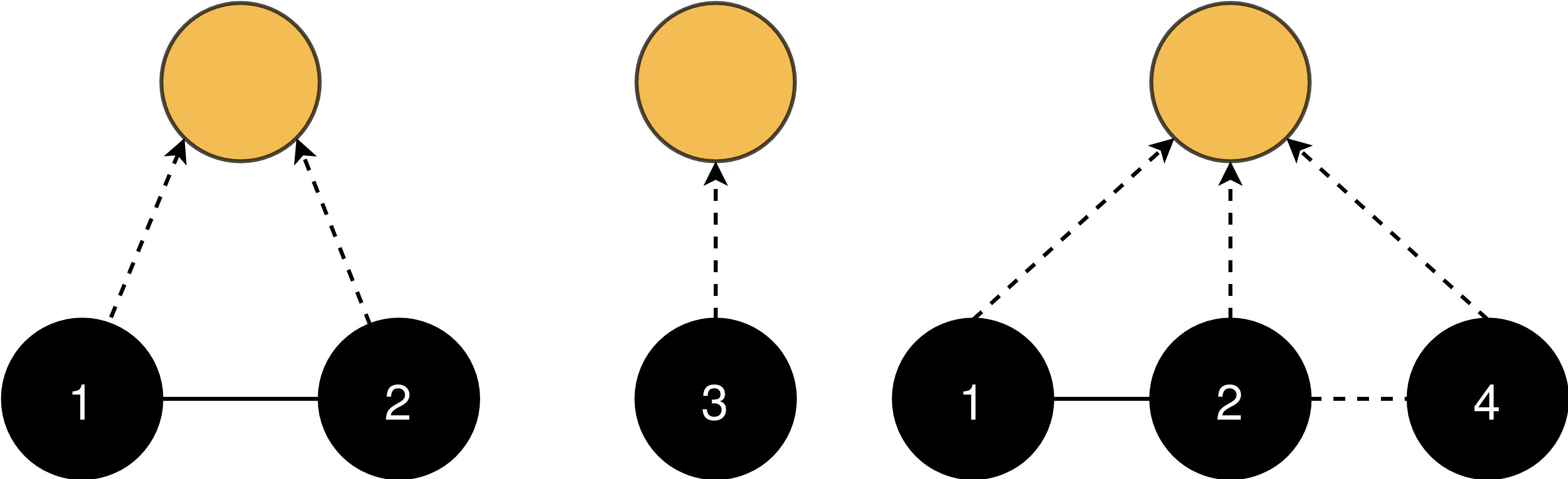
Figure 4: The coarsening process. Original and coarse nodes are colored in black and yellow, respectively. Dashed arrow indicates parent-child relationship. Solid line represents heaviest-weighted edge. Left: A coarse node is created from two adjacent nodes $1$ and $2$. Middle: A coarse node is created from a true singleton node $3$. Right: A left-over singleton node $4$ is attached to a coarse, nearest neighbor node $2$.

2.3 Coarsening approach: Independent sets

It is also possible to exploit independent sets (see, e.g., [95]) for coarsening graphs. Recall that an independent set $\mathcal{S}$ is a subset of $V$ that consists of nodes that are not adjacent to each other; i.e., no pair $(v,w)$ where $v,w\in\mathcal{S}$ is linked by an edge. An independent set $\mathcal{S}$ is maximal if no (strict) superset of $\mathcal{S}$ forms another independent set. One can use the nodes of a carefully selected independent set to form a coarse graph; i.e., we can define $V_{c}=\mathcal{S}$. Then, it is relatively easy to determine the edges and weights between these nodes by using information from the original graph. For example, in [95] an edge is inserted between $v$ and $w$ of $V_{c}$ if there is at least one node $y$ in $V\backslash V_{c}$ such that $(v,y)\in E$ and $(w,y)\in E$. This will produce the edge set $E_{c}$ needed to form the coarse graph $G_{c}$.

Let $L$ be the graph Laplacian, reordered such that the $n_{c}$ nodes of $V_{c}$ are listed first. Then $L$ will have the following structure, where $D_{c}\ \in\ \mathbb{R}^{n_{c}\times n_{c}}$ :

(12) $$L=\begin{pmatrix}D_{c}&-F\\ -F^{T}&B\end{pmatrix}.$$

Since the nodes associated with the (1,1) block in the above matrix form an independent set, it is clear that the matrix $D_{c}$ is diagonal. Coarsening by independent sets will consist of taking the matrix $D_{c}$ and adding off diagonal elements to it to obtain the adjacency matrix $A_{c}$. An important observation to be made here is that the edges added by the independent set coarsening are those obtained from the Schur complement with respect to $B$, where $B$ is replaced by a diagonal matrix. Let us assume that $B$ is replaced by a matrix $D_{f}$. The resulting Schur complement is

(13) $$S_{c}=D_{c}-FD_{f}^{-1}F^{T}.$$

The nonzero pattern of $S_{c}$ is the same as that of $FF^{T}$, which is in turn the sum of the patterns of $f_{j}f_{j}^{T}$ where $f_{j}$ is the $j$-th column of $F$. If $f_{j}$ has nonzero entries in locations $i$ and $k$, then we will have nonzero entries in the positions $(i,i),(i,k),(k,i)$ and $(k,k)$ of $S_{c}$. Next, we will define $D_{f}$ more specifically. Let $D_{f}$ be the diagonal of row-sums of $F^{T}$ and assume for now that these are all nonzero. This is the same diagonal as the one used for the graph Laplacian except that the summation ignores the entries $a_{ij}$ when $i$ and $j$ are both in $V\backslash V_{c}$. In matlab notation: $D_{f}=\mbox{diag}(\mbox{diag}(F^{T}\mathbf{1}))$. In this situation, $S_{c}$ becomes a Laplacian.

Proposition 2.1.

Let $B$ be replaced by $D_{f}$, defined as the diagonal of the row-sums of $F^{T}$. Then $D_{f}$ is invertible. Let $L_{c}=D_{c}-FD_{f}^{-1}F^{T}$. Then the graph of $L_{c}$ is $G_{c}$, the graph of the independent set coarsening of $G$. In addition, $L_{c}$ is a graph Laplacian; specifically, it is the graph Laplacian of $G_{c}$.

Proof 2.2.

Because the independent set is maximal, we cannot have a zero diagonal element in $D_{f}$. Indeed, if the opposite was true, then one row, say row $k$, of $F^{T}$ would be zero. This would mean that we could add node $k$ to the independent set, because it is not coupled with any element of $\mathcal{S}$. The result would be another independent set that includes $\mathcal{S}$, contradicting maximality.

It was shown above that the adjacency graph of $FF^{T}$, which is the same as that of $L_{c}$, is exactly $G_{c}$. It is left to show that $L_{c}$ is a Laplacian. Since $D_{f}$ and $F$ have nonnegative entries, the off-diagonal of $L_{c}$ are clearly negative. Next, note that $F^{T}\mathbf{1}=D_{f}\mathbf{1}$ and hence

$$(D_{c}-FD_{f}^{-1}F^{T})\mathbf{1}=D_{c}\mathbf{1}-FD_{f}^{-1}D_{f}\mathbf{1}=(D_{c}-F)\mathbf{1}=0.$$

Thus, $L_{c}$ is indeed a Laplacian.

2.4 Coarsening approach: Algebraic distance

Researchers in AMG methods defined a notion of ‘algebraic distance’ between nodes based on relaxation procedures. This notion is motivated by the bootstrap AMG (BAMG) method [25] for solving linear systems. AMG creates a coarse problem by trying to exploit some rules of ‘closeness’ between variables. In BAMG, this notion of closeness is defined from running a few steps of Gauss-Seidel relaxations, starting with some random initial guess for solving the related homogeneous system $Ax=0$. The speed of convergence of the iterate determines the closeness between variables. This is exploited to aggregate the unknowns and define restriction and interpolation operators [97]. In [36] this general idea was extended for use on graph Laplacians. In the referenced paper, Gauss-Seidel is replaced by Jacobi overrelaxation.

Algorithm 2 Algebraic distances for graphs

1:Input: Parameter $\omega$, weighted graph $G=(V,E,A)$, initial vector $x^{(0)}$, number of steps $k$.

2:Output: Distances $s_{ij}^{(k)}$ for each pair $(i,j)$.

3:for $j=1,2,\cdots,k$ do

4:     $x^{(j)}=(1-\omega)x^{(j-1)}+\omega D^{-1}Ax^{(j-1)}$

5:end for

6:Set: $s_{ij}^{(k)}=|x_{i}^{(k)}-x_{j}^{(k)}|\,\,\forall i,j$

Algorithm 2 shows how these distances are calculated. They depend on two parameters: the over relaxation parameter $\omega$ and the number of steps, $k$. It can be shown that the distances $s_{ij}^{(k)}$ converge to zero [36] as $k\rightarrow\infty$. However, it was argued in [36] that the speed of decay of $s_{ij}^{(k)}$ is an indicator of relative strength of connection between $i$ and $j$. In other words, the important measure is the magnitude – in relative terms – of $s_{ij}^{(k)}$ for different $(i,j)$ pairs.

Note that the iteration is of the form $x^{(j)}=Hx^{(j-1)}$, where $H$ is the iteration matrix

$$H=(1-\omega)I+\omega D^{-1}A=I-\omega(I-D^{-1}A).$$

Because $D-A$ is a graph Laplacian, the largest eigenvalue of $H$ is $\lambda_{1}=1$. It is then suggested to scale these scalars by $\lambda_{2}^{k}$, where $\lambda_{2}$ is the second largest eigenvalue in modulus. In general, it is sufficient to iterate for a few steps and stop at a step $k$ when one observes the scaled quantities start to settle.

As can be seen, a coarsening method based on algebraic distances is rather different from the previous two methods. Instead of working on the graph directly we now use our intuition on the iteration matrix to extract intuitive information on what may be termed a relative distance between variables. If two variables are close with respect to this distance, they may be aggregated or merged.

Ultimately, as was shown in [36], what is important is the decay of the component of the vector $x^{(k)}-x^{(k-1)}$ in the second eigenvector. This distance between two vectors is indeed dominated by the component in the second eigenvector.

This brings up the question as to whether or not we can directly examine spectral information and infer from it a notion of distance on nodes. Spectral graph coarsening addresses this and will be examined in Section 4.

2.5 Techniques related to coarsening

Graph coarsening is a graph reduction technique, in the sense that it aims at reducing the size of the original graph while attempting to preserve its properties. There exist a number of other techniques in the same category. These include graph summarization [85, 74], graph compression [50], and graph sketching  [70]. These are more common in machine learning and the tasks they address are specific to the underlying applications. In the following we discuss methods that are more akin to standard coarsening methods.

2.5.1 Graph reduction: Kron

The Kron reduction of networks was proposed back in 1939 [71], as a means to obtain lower dimensional electrically equivalent circuits in circuit theory. Its popularity gained momentum across fields after the appearance of a thorough analysis of the method in [46]. The method starts with a weighted graph $G=(V,E,A)$ and the associated graph Laplacian $L$, along with a set $V_{1}$ of nodes which is a strict subset of $V$. Such a subset can be obtained by downsampling, for example, although in the original application of circuits it is a set of nodes at the boundary of the circuit. The method essentially defines a coarse graph from the Schur complement of the original adjacency graph with respect to this downsampled set.

The goal is to form a reduced graph on $V_{1}$. This is viewed from the angle of Laplacians. If we order the nodes of $V_{1}$ first, followed by those of the complement set to $V_{1}$ in $V$, the Laplacian can be written in block form as follows:

(14) $$L=\begin{bmatrix}L_{11}&L_{12}\\ L_{12}^{T}&L_{22}\end{bmatrix}.$$

The Kron reduction of $L$ is defined as the Schur complement of the original Laplacian relative to $L_{22}$; i.e.,

(15) $$L(V_{1})=L_{11}-L_{12}L_{22}^{-1}L_{12}^{T}.$$

This turns out to be a proper graph Laplacian as was proved in [46], along with a few other properties. We can therefore associate a set of weights $A_{ij}^{(1)}$ for the reduced graph, defined from $L(V_{1})$:

$$a_{ij}^{(1)}=\left\{\begin{array}[]{cl}-[L(V_{1})]_{ij}&\mbox{if }i\neq j,\\ 0&\mbox{otherwise}.\end{array}\right.$$

An example is shown in Figure 5.

A multiscale version of the Kron reduction, called the pyramid transform, was proposed in [108], specifically for applications that involve signal processing on graphs [109]. It was developed as a multiscale (i.e., ‘multilevel’ in the scientific computing jargon) extension of a similar scheme invented in the late 1980s for image processing [31]. The extension is from regular data (discrete time signals, images) to irregular data (graphs, networks) as well as from one level to multiple levels.

An original feature of the paper [108] is the use of spectral information for coarsening the graph. Specifically, a departure from traditional coarsening methods such as those described in Sections 2.2 and 2.3 is that the separation into coarse and fine nodes is obtained from the ‘polarity’ (i.e., the sign of the entries) of the eigenvector associated with the largest eigenvalue of the graph Laplacian. The motivation of the authors is a theorem by Roth [98], which deals with bipartite graphs. The idea of exploiting spectral information was exploited earlier by Aspvall and Gilbert [3] for the problem of graph coloring, an important ingredient of many linear algebra techniques. Another original feature of the paper [108] is the use of spectral methods for sparsifying the Schur complement. As was mentioned earlier, the Schur complement will typically be dense, if not full in most situations. The authors invoke ‘sparsification’ to reduce the number of edges. We will cover sparsification in Section 2.5.3.

Example

As an example, we return to the illustration of Figure 5. Using normalized Laplacians, we find that the largest eigenvector separates the graph in two parts according to its polarity, namely $V_{1}=\{1,5,6,9,10\}$ and $V_{2}=\{2,3,4,7,8,11\}$. Thus, it is able to discover $V_{1}$, the rather natural independent set we selected earlier.

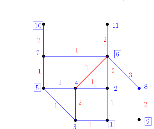
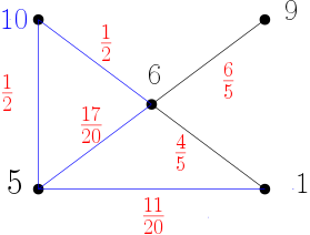
Figure 5: A small graph (left) and its Kron reduction (right). The reduced set of nodes is $V_{1}=\{1,5,6,9,10\}$. These node labels are kept in the Kron reduction. Numbers on the middle of the edges are the weights.

One important question that can be asked is why resort to the Schur complement as a means of graph reduction? A number of properties regarding the Kron reduction were established in [46] to provide justifications. Prominent among these is the fact that the resistance distance [49] between nodes of the coarse graph are preserved. The resistance distance involves the pseudo-inverse of the Laplacian.

2.5.2 Relationship between Kron reduction and independent set coarsening

Instead of invoking independent sets, the Kron reduction, as it is used in [108], ‘downsamples’ nodes by means of spectral information. While these samples may form an independent set, this is not guaranteed. Just like independent set coarsening, the coarse graph is built from the Schur complement associated with the complement of the independent set (so-called node cover). These two ways of coarsening are illustrated in Figure 6.

Unlike independent set coarsening, the matrix $L_{22}$ involved the Schur complement of (15) is not approximated by a diagonal before inversion, in effort to reduce the fill-ins introduced. Instead, spectral ‘sparsification’ is invoked. In the survey paper [46], the set $V_{1}$ represents a set of ‘boundary points’ in an electrical network. Improved sparsity is achieved by other means than those employed in Section 2.3, specifically by eliminating a selection of internal nodes instead of all of them, in the Gaussian elimination process.

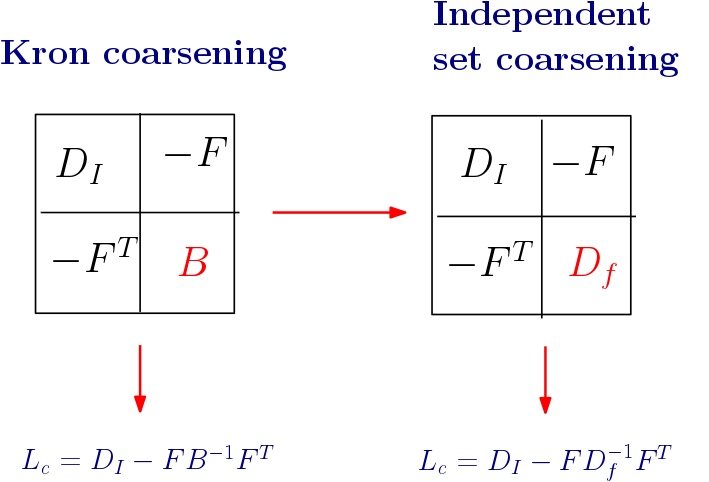
Figure 6: Two ways of using independent sets for coarsening.

2.5.3 Graph sparsification

Graph sparsification methods aim at finding a sparse approximation of the original graph by trimming out edges from the graph [112, 111]. Here, the number of nodes remains the same but the number of edges, $|E|$, can be much lower than in the original graph. This is motivated by the argument that in some applications, the graphs that model the data tend to be rather dense and that many edges can be removed without negatively impacting the result of methods that exploit these graphs; see, e.g., [64].

Different measures of closeness between the sparsified and the original graph have been proposed for this purpose, resulting in a wide range of strategies such as spanners [2], cut sparsifiers [65], and spectral sparsifiers [112]. Graph sparsification methods can be beneficial when dealing with high density graphs and come with rigorous theoretical guarantees [13]; see also [16].

We already mentioned at the end of Section 2.5.1 one specific use of graph sparsifiers in the context of multilevel graph coarsening. To sparsify the successive Schur complement obtained by the multilevel scheme, the authors of [108] resorted to a spectral sparsifier developed in [111]. If $\widetilde{G}$ is the sparsified version of $G$, and if $\widetilde{L}$ and $L$ are their respective Laplacians, the main goal of spectral sparsifiers is to preserve the quadratic form associated with the Laplacians. The graph $\widetilde{G}$ is said to be a $\sigma$-spectral approximation of $G$ if for all $x\ \in\ \mathbb{R}^{n}$,

(16) $$\frac{1}{\sigma}x^{T}\widetilde{L}x\leq x^{T}Lx\leq\sigma\ x^{T}\widetilde{L}x.$$

A trivial observation for $\sigma$-similar ($\sigma>1$) graphs is that their Rayleigh quotients

$$\mu(x)=\frac{(Lx,x)}{(x,x)}\ ,\qquad\widetilde{\mu}(x)=\frac{(\widetilde{L}x,x)}{(x,x)}$$

for the same nonzero vector $x$ satisfy the double inequality:

(17) $$\frac{1}{\sigma}\ \widetilde{\mu}(x)\leq\mu(x)\leq\sigma\ \widetilde{\mu}(x).$$

Thus, these Rayleigh quotients are, in relative terms, within a factor of $\sigma-1$ of each other:

$$\left|\frac{\widetilde{\mu}(x)-\mu(x)}{\widetilde{\mu}(x)}\right|\leq\sigma-1.$$

This has an impact on eigenvalues. If $\sigma$ is close to one, then clearly the eigenvalues of $L$ and $\widetilde{L}$ will be close to each other, thanks to the Courant–Fisher min-max characterization of eigenvalues [54]. In what follows, $S_{k}$ represents a generic $k$-dimensional subspace of $\mathbb{R}^{n}$ and eigenvalues are sorted decreasingly. In this situation, the theorem states that the $k$-th eigenvalue of the Laplacian $L$ satisfies:

(18) $$\lambda_{k}=\max_{\text{dim}(S_{k})=k}\quad\min_{0\neq x\in S_{k}}\mu(x).$$

The above maximum is achieved by a set, denote by $S_{*}$ (which is just the linear span of the set of eigenvectors $u_{1},\cdots,u_{k}$). Then

$$\lambda_{k}=\min_{0\neq x\in S_{*}}\ \mu(x)\,\,\leq\,\,\min_{0\neq x\in S_{*}}\ \sigma\widetilde{\mu}(x)\,\,\leq\,\,\sigma\max_{S_{k}}\min_{0\neq x\in S_{k}}\ \widetilde{\mu}(x)\,\,\leq\,\,\sigma\ \widetilde{\lambda}_{k}.$$

The exact same relation as (16) holds if $L$ and $\widetilde{L}$ are interchanged. Therefore, the above relation also holds if $\lambda$ and $\widetilde{\lambda}$ are interchanged, which leads to the following double inequality, valid for $k=1,2,\cdots,n$:

(19) $$\frac{\widetilde{\lambda}_{k}}{\sigma}\leq\lambda_{k}\leq\sigma\widetilde{\lambda}_{k}.$$

It is also interesting to note a link with preconditioning techniques. When solving symmetric positive definite linear systems of equations, it is common to approximate the original matrix $A$ by a preconditioner which we denote here by $\widetilde{A}$. Two desirable properties that must be satisfied by a preconditioner $\widetilde{A}$ are that (i) it is inexpensive to apply $\widetilde{A}^{-1}$ to a vector; and (ii) the condition number of $\widetilde{A}^{-1}A$ is (much) smaller than that of $A$. The second condition translates into the condition that $(Ax,x)/(\widetilde{A}x,x)$ be small. If we assume that

(20) $$\frac{1}{\sigma}\leq\frac{(Ax,x)}{(\widetilde{A}x,x)}\leq\sigma,$$

then the condition number of the preconditioned matrix, which is the ratio of the largest to the smallest eigenvalues of $\widetilde{A}^{-1}A$, will be bounded by $\sigma^{2}$.

2.5.4 Graph partitioning

The main goal here is to put in contrast the problem of coarsening with that of graph partitioning. To his end, a brief background is needed. In spectral graph partitioning [51, 12, 91], the important equality (3) satisfied by any Laplacian $L$ is exploited. If $x$ is a vector of entries $+1$ or $-1$, encoding membership of node $i$ to one of two subgraphs, then the value of $x^{T}Lx$ is equal to 4 times the number of edge cuts between the two graphs with this 2-way partitioning. We could try to find an optimal 2-way partitioning by minimizing the number of edge cuts, i.e., by minimizing $x^{T}Lx$ subject to the condition that the two subgraphs are of equal size, i.e., subject to $\mathbf{1}^{T}x=0$. Since this optimization problem is hard to solve, it is common to ‘relax’ it by replacing the conditions $x\in\{-1,1\}^{n},x^{T}\mathbf{1}=0$ with $x\in\mathbb{R}^{n},\|x\|=1,x^{T}\mathbf{1}=0$. This leads to the definition of the Fiedler vector, which is the second smallest eigenvector of the Laplacian. Recall that the smallest eigenvalue of the graph Laplacian is zero and that when the graph is connected, this eigenvalue is simple and the vector $\mathbf{1}$ is a corresponding eigenvector.

It is interesting to note the similarity between spectral graph partitioning and Kron reduction. In both cases, the polarity of an eigenvector is used to partition the graph in two subgraphs. In the case of Kron reduction, it is the vector associated with the largest eigenvalue that defines the partitions; and one of these partitions is selected as the ‘coarse’, or the ‘downsampled’ set, according to the terminology in [108]. For graph partitioning, what is done instead is to use the eigenvector at the other end, the one next to the smallest, since the smallest is a constant vector. If we reformulate the problem back in terms of assignment labels of $\pm 1$, then this would lead to the interpretation that in one case, we try to minimize edge cuts (partitioning) and in the other, we try to maximize them (Kron reduction).

An illustration is shown in Figure 7 with a small finite element mesh. As can be seen, using the second smallest eigenvector tends to color the graph in such a way that nearest neighbors of a node are mostly of the same color, while using the largest eigenvector tends to color the graph in such a way that nearest neighbors of a node are mostly of a different color. Another way to look at this is that using the second smallest eigenvector gives domains that tend to be ‘fat’ whereas the largest eigenvector gives domains that tend to be ‘thin’, like unions of lines separating each other. Another fact shown by this simple example is that neither of the two sets obtained is close to being an independent set.

The following property is straightforward to prove.

Proposition 2.3.

Assume that the graph has no isolated node and that the components $\xi_{1},\xi_{2},\cdots,\xi_{n}$ of the largest eigenvector $u_{1}$ are nonzero. Let $V_{+}$ and $V_{-}$ be the two subgraphs obtained from the polarities of the largest eigenvector. Then each node of $V_{+}$ (resp. $V_{-}$) must have at least one adjacent node from $V_{-}$ (resp. $V_{+}$).

Proof 2.4.

The $i$-th row of the relation $Lu_{1}=\lambda_{1}u_{1}$ yields: (recall definition (2))

$$d_{i}\xi_{i}-\sum_{j\in\ N(i)}a_{ij}\xi_{j}=\lambda_{1}\xi_{i}\quad\rightarrow\quad(\lambda_{1}-d_{i})\xi_{i}=-\sum_{j\in\ N(i)}a_{ij}\xi_{j}.$$

Note that $(\lambda_{1}-d_{i})>0$ (due to assumption). Then, if $\xi_{i}\neq 0$ (left side) then at least one of the $\xi_{j}$’s, $j\neq i$ (right side) must be of the opposite sign.

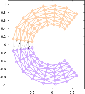
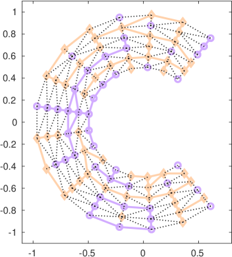
Figure 7: Subgraphs from eigenvectors of the (normalized) Laplacian. Left side: using second smallest eigenvector; Right side: using largest eigenvector. The two sets are colored differently and edge-cuts are shown as dotted lines.

3 Graph coarsening in machine learning

In this section, we discuss existing methods related to graph coarsening in machine learning and discuss how they are employed in typical applications. We begin by defining the types of problems encountered in machine learning and the related terminology. The terms ‘graphs’ and ‘networks’ are often used interchangeably in the literature – although the term networks is often employed specifically for certain types of applications, whereas graphs are more general. For example, ‘social networks’ are common for applications that model friendship or co-authorship, while one speaks of graphs when modeling chemical compounds. What muddles the terminology is the term ‘graph neural networks,’ which are neural networks (a type of machine learning model) for graphs. Furthermore, there are ‘protein-protein interaction networks,’ which are graphs of proteins; that is, each graph node is a protein, which by itself is a molecular graph.

Some commonly encountered graph tasks include: node classification (determine the label of a node in a given graph), link prediction (predict whether or not an edge exists between a pair of nodes), graph classification (determine the label of the graph itself), and graph clustering (group nodes that are most alike together). One of the key concepts in a majority of the methods for solving these tasks is embedding, which is vector in $\mathbb{R}^{d}$ used to represent a node $v\in V$ or indeed the entire graph $G=(V,E)$.

3.1 Graph clustering and GraClus

As was seen earlier, graph coarsening is a basic ingredient of graph partitioning. The same graph partitioning tools can be used in data-related applications, but the requirement of having partitions of equal size is no longer relevant. This observation led to the development of approaches specifically for data applications; see, e.g., [43]. The method developed in [43] uses a simple greedy graph coarsening approach whereby nodes are visited in a random order. When visiting a node, the algorithm merges it with the unvisited nearest neighbor that maximizes a certain measure based on edge and node weights. The visited node and the selected neighbor are then marked as visited. The algorithm developed in [43], which is known as GraClus, uses different tools from those of graph partitioning. Because it is used for data applications, the refinement phase exploits a kernel K-means technique instead of the usual Kernighan–Lin procedure [67].

3.2 Multilevel graph coarsening for node embedding

In one form of node embedding, one seeks a mapping $\Phi$ from the node set $V$ of a graph $G=(V,E)$ to the space $\mathbb{R}^{n\times d}$ where $n=|V|$ and

(21) $$\Phi:v\in V\longrightarrow\Phi(v)\ \in\ \mathbb{R}^{d}.$$

In other words, each node is mapped to a vector in $d$-dimensional space. Here, the dimension $d$ is usually much smaller than $n$. Many embedding methods have been developed and used effectively to solve a variety of problems; see, e.g., [99, 14, 1, 114, 33, 56, 122, 35] and [55] for a survey. The idea of applying coarsening to obtain embedding for large graphs has been gaining ground in recent years; see, [35, 73, 42, 93].

The authors of [35] present a method dubbed hierarchical representation learning for networks (HARP), which exploits coarsening to facilitate and improve graph embedding. The method starts by performing a sequence of $\ell$ graph coarsening steps to produce graphs $G_{1},G_{2},\cdots,G_{\ell}$ from the initial graph $G_{0}$. Then, an embedding is performed on the final level to produce the mapping $\Phi_{\ell}$. This embedding is then propagated back to the original level by proceeding as follows. Starting from level $i=\ell$, the mapping $\Phi_{i}$ is naturally prolongated (‘extrapolated’) from level $i$ to level $i-1$ to yield a mapping $\Phi_{i-1}^{\prime}$. An extra step is taken to refine this embedding and obtain $\Phi_{i-1}$. This specific step is rather reminiscent of the ‘post-smoothing’ steps invoked in various MG schemes for solving linear systems. Post-smoothing consists of a few steps of smoothing operations, typically a standard relaxation method (e.g., Gauss-Seidel), applied after an approximate solution is prolonged from a coarse level. The MILE method described in [73] is rather similar to the HARP approach described above, the main difference being that the refinement proposed in this method exploits neural networks.

HARP and MILE are general frameworks that use coarsening to improve graph embedding. In the remainder of this section, we give an illustrative example to demonstrate the effectiveness of HARP. We examine the performance improvement of three widely used graph embedding algorithms: DeepWalk [90], LINE [114], and Node2vec [56], each combined with HARP. Furthermore, because HARP is a general framework and we have the freedom to choose the coarsening method it uses, we examine the impact of different coarsening methods on the performance improvement. Three coarsening methods are tested: HEM (Section 2.2), algebraic distance (Section 2.4), and the LESC method to be introduced in Section 5 (it is similar to HEM but uses spectral information to define the visiting order of nodes).

We evaluate the HARP framework on a node classification task with the Citeseer graph [106]. Citeseer is a citation graph of computer science publications, consisting of 3.3K nodes and 4.5K edges. The label of each node indicates the subject area of the paper. The task is to predict the labels. We first generate the node embedding for each node using the HARP method. Then, a fraction of the nodes are randomly sampled to form the training set and the remaining is used for testing. We train a logistic regression model [20] by using the training data and evaluate the classification performance on the test data. We use the macro-average F1 score [92] as the performance metric, which is the mean of the F1 score for each label category. Figure 8 shows the score under different training set sizes.

As can be seen the HARP framework consistently improves all these embedding methods, especially LINE and DeepWalk. Each coarsening approach used inside the HARP framework improves the performance to a different degree, with the LESC approach generally outperforming the others.

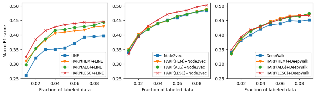
Figure 8: Classification results on the Citeseer graph. The x-axis shows the portion of nodes used for training. The y-axis shows the macro-average F1 score. Each reported score is an average over five random repetitions.

3.3 Graph neural networks and graph pooling

GNNs have recently attracted a great deal of interest in various disciplines, including biology [44], chemistry [121], and social networks [124], where data is modeled by graphs. A major class of GNNs are those of a convolution style that generalize lattice convolutions in convolutional neural networks (CNNs). A standard convolution applies a filter on a signal; in CNNs, the signal is a 2-dimensional image and the filter has a very small support—say, a $3\times 3$ window. Convolution-style GNNs generalize the regularity of such a filter to irregularly connected node pairs [29, 59, 82]. Specifically, the regular window is replaced by the 1-hop neighborhood of a node.

One such representative GNN is the graph convolutional network (GCN) [68]. GCN maps a feature matrix $X$ to the label matrix $Y$ (see notation introduced in Section 1.2) by including the graph adjacency matrix $A$ in the mapping:

(22) $$\widetilde{Y}=\operatorname{softmax}(\widehat{A}\cdot\operatorname{ReLU}(\widehat{A}XW^{0})\cdot W^{1}),$$

where $\widehat{A}$ is a normalization of $A$ through $\widehat{A}=\widetilde{D}^{-1/2}\widetilde{A}\widetilde{D}^{-1/2}$, $\widetilde{A}=A+I$, $\widetilde{D}=\mbox{diag}(\widetilde{d}_{i})$, and $\widetilde{d}_{i}=\sum_{j}\widetilde{a}_{ij}$. Therefore, matrix products such as $\widehat{A}X$ denote the convolution by using a 1-hop neighborhood filter.

The following concepts are for neural networks. The functions $\operatorname{ReLU}$ and $\operatorname{softmax}$ are nonlinear activation functions: $\operatorname{ReLU}(x)=\max\{x,0\}$ is an elementwise function, while $\operatorname{softmax}(x)=[e^{x_{1}}/c,\ldots,e^{x_{d}}/c]$ with $c=\sum_{j}e^{x_{j}}$ is a vector function; it acts on each row if the input is a matrix. The matrices $W^{0}$ and $W^{1}$ are called weight matrices. Their sizes are uniquely determined by the sizes of the other matrices in (22). Their contents are not manually specified but learned through minimizing the discrepancy between $\widetilde{Y}$ and the ground truth label matrix $Y$.

Besides GCN, the literature has seen a large number of generalizations of lattice convolution to convolutions in the graph context, including for example, spectral [30, 60, 68, 41] and spatial [87, 58, 120, 126, 123, 83] schemes.

GNNs such as (22) essentially produce a mapping $\Phi:v\in V\longrightarrow\Phi(v)\ \in\ \mathbb{R}^{c}$ for every node $v$ in the graph, if we read only one row of $\widetilde{Y}$ in (22). This mapping is almost identical to the form (21) discussed in the context of node embedding; the only nominal difference is that the output is in a $c$-dimensional space while the node embedding is in $d$-dimensional space. This difference is caused by the need for the output $\widetilde{Y}$ to be matched with the ground truth $Y$ that has $c$ columns ($c$ label categories); while for node embedding, the embedding dimension $d$ may be arbitrary. However, if our purpose is not to match $\widetilde{Y}$ with $Y$, we can adjust the number of columns of $W^{1}$ so that the right-hand side of (22) can be repurposed for producing a node embedding. More significantly, we may take the elementwise minimum, the average, or the weighted average of the node embedding vectors to form an embedding vector for the entire graph $G=(V,E)$ [48]. In other words, a GNN, with a slight modification, can produce a mapping

(23) $$\Psi:G\longrightarrow\Psi(G)\ \in\ \mathbb{R}^{d}.$$

Now that we see how GNNs can be utilized to produce a graph embedding through the mapping $\Psi$, a straightforward application of coarsening is to use $\Psi(G_{c})$ in place of $\Psi(G)$ for the classification of $G$. This simple idea can be made more sophisticated in two ways. First, suppose we perform a multilevel coarsening resulting in a sequence of increasingly coarser graphs $G=G_{0},G_{1},G_{2},\ldots,G_{\ell}$. We may concatenate the vectors $\Psi(G_{0}),\Psi(G_{1}),\ldots,\Psi(G_{\ell})$ and treat the resulting vector as the embedding of $G$. We use the concatenation result (say $\psi_{G}$) to classify $G$, though building a linear classifier that takes $\psi_{G}$ as input and outputs the class label.

Second, we introduce the concept of pooling. Pooling in neural networks amounts to taking a min/max or (weighted) average of a group of elements and reducing it to a single element. In the context of graphs, pooling is particularly relevant to coarsening, since if we recall the Galerkin projection $f^{(\ell+1)}=P_{\ell}^{T}f^{(\ell)}$ in AMG (see (8)), the interpolation matrix $P_{\ell}$ plays the role of pooling: each column of $P_{\ell}$ defines the weights in the averaging of nodes in the last graph into a node in the coarse graph. Hence, in the context of GNNs, we call $P_{\ell}$ a pooling matrix. This matrix can be obtained directly through the definition of a coarsening method [41, 110], or it can be unspecified but learned through training [125, 52, 72]. By using successive poolings that form a hierarchy, recent work [125, 72, 52, 69] has shown that hierarchical pooling improves graph classification performance.

4 Spectral coarsening

While the terms ‘spectral graph partitioning’ and ‘spectral clustering’ are quite well-known, the term ‘spectral graph coarsening’ is less explored in the literature. There are two aspects, and therefore possible directions, to spectral coarsening. First, it may be desirable in various tasks to preserve the spectral properties of the original graph, as is the case in the local variation method proposed by [75]. The second aspect is that one may wish to apply spectral information for coarsening. The method proposed by [108] falls in this category. It uses the eigenvector of the graph Laplacian to select a set of nodes for Kron reduction [46] discussed earlier.

In this section, we present an approach for the first aspect; whereas in Section 5, we develop an approach related to the second aspect. Regarding the first aspect, eigenvectors of the graph Laplacian encapsulate much information on the structure of the graph. For example, the first few eigenvectors are often used for partitioning the graph into more or less equal partitions. Therefore, the first question we will ask is whether or not it is possible to coarsen a graph in such a way that eigenvectors are ‘preserved.’ Of course, the coarse graph and the original one have different sizes so we will have to clarify what is meant by this.

4.1 Coarsening and lifting

Recall from AMG that coarsening is represented by the matrix $P\in\mathbb{R}^{n\times n_{c}}$. It helps to view a coarse node as a linear combination of a set of nodes in the original graph. Let the $k$-th coarse node be denoted by $v_{k}^{(c)}$ and the set be $S_{k}$. The weights are $p_{ik}$ for each $v_{i}\in S_{k}$:

(24) $$v_{k}^{(c)}=\sum_{v_{i}\in S_{k}}p_{ik}v_{i}.$$

In the simplest case, we can let $p_{ik}=1/|S_{k}|$ for all $v_{i}\in S_{k}$. The coarse adjacency matrix is then defined as:

(25) $$A_{c}=P^{T}AP.$$

A similar framework of writing a coarsened matrix in the form of (25) is adopted in [75]. Note that in general, $A_{c}$ is not binary. Here, we assign the diagonal entries of $A_{c}$ to $0$ and all non-zero entries to $1$.

The original graph $G$ and its coarse graph $G_{c}$ have a different number of nodes. If we wish to compare the properties of these two graphs, it is necessary to ‘lift’ the graph Laplacian of $G_{c}$ into a matrix that has the same size as that of $G$. Let $L$ and $L_{c}$ denote the Laplacian of the original graph and the coarse graph, respectively. One way to construct a matrix $L_{c}$ that is guaranteed to be a graph Laplacian is as follows [75, 63]:

(26) $$L_{c}=C^{T}LC,$$

where $C\in\mathbb{R}^{n\times n_{c}}$ is a sparse matrix with

(27) $$C_{ij}=\begin{cases}1,&\text{node $i$ in }S_{j},\\ 0,&\text{otherwise}.\end{cases}$$

Note that the matrix $P$ defined in (24) is the pseudoinverse of $C^{T}$, with $C^{T}P=I_{n_{c}}$. Therefore, the lifted counterpart of $L_{c}$, denoted by $L_{l}$, is defined as

(28) $$L_{l}=PL_{c}P^{T},$$

because $PC^{T}$ is a projector.

4.2 The projection method viewpoint

If we extend the matrix $P$ as an orthonormal matrix, then $PP^{T}$ is a projector and the lifted Laplacian defined in (28) becomes $L_{l}=PP^{T}LPP^{T}$. It is useful to view spectral coarsening from the projection method [103] angle.

Consider an orthogonal projector $\pi$ and a general (symmetric) matrix $A$. In an orthogonal projection method on a subspace $\mathcal{V}$, we seek an approximate eigenpair $\tilde{\lambda},\tilde{u}$, where $\tilde{u}\ \in\ \mathcal{V}$ such that

$$\pi(A-\tilde{\lambda}I)\tilde{u}=0.$$

If $V=[v_{1},v_{2},\cdots,v_{k}]$ is an orthonormal basis of $\mathcal{V}$ and the approximate eigenvector is written as $\tilde{u}=Vy$, then the previous equation immediately leads to the problem

(29) $$V^{T}AVy=\lambda y.$$

The eigenvalue $\tilde{\lambda}$ is known as a Ritz value and $\tilde{u}$ is the associated Ritz vector.

Recall the orthogonal projector $\pi$ onto the columns of $P$; that is, $\pi=PP^{T}$. If we look at the specific case under consideration, we notice that this is precisely what is being done and that the basis vectors $V$ are just the columns of $P$.

When analyzing errors for projection methods, the orthogonal projector $\pi$ represented by the matrix $PP^{T}$ plays a particularly important role. Specifically, a number of results are known that can be expressed based on the distance $\|(I-\pi)u\|$ where $u$ is an eigenvector of $A$; see, e.g., [103]. The norm $\|(I-\pi)u\|$ represents the distance of $u$ to the range of $\pi$ in $\mathbb{R}^{n}$.

4.3 Eigenvector preserving coarsening

Based on the interpretation of projection methods, it is desirable to construct a projector that preserves eigenvectors. We say that a given eigenvector $u$ is exactly preserved or just ‘preserved’ by the coarsening if $(I-\pi)u=0$. If this is the case then when we solve the projected problem (29), we will find that $y=P^{T}u$ is an eigenvector of $V^{T}AV$ associated with the eigenvalue $\lambda$:

$$V^{T}AV(V^{T}u)=V^{T}A\pi u=V^{T}Au=\lambda V^{T}u.$$

The Ritz vector is $\tilde{u}=Py=PP^{T}u=\pi u=u$, which is clearly an eigenvector.

What might be more interesting is the more practical situation in which $(I-\pi)u$ is not zero but just small. In this case, there are established bounds [103] for the angle between the exact and approximate eigenvectors based on the quantity $\epsilon=\|(I-\pi)u\|$.

In what follows, we instantiate the general matrix $A$ by the graph Laplacian matrix $L$ and consider the preservation of its eigenvectors. From many machine learning methods (e.g., the Laplacian eigenmap [15]), the bottom eigenvectors of $L$ carry the crucial information of a dataset. Thus, they are the ones that we want to preserve.

4.4 Preserving one eigenvector

If we want to coarsen the graph into $k$ nodes, we partition an eigenvector $u$ into $k$ parts. Up to permutations of the elements of $u$, let us write, in matlab notation

$$u=\begin{bmatrix}u_{1}\ ;\ u_{2}\ ;\ \cdots\ ;\ u_{k}\end{bmatrix}.$$

Then, we let

$$P=\begin{bmatrix}u_{1}/\|u_{1}\|\\ &u_{2}/\|u_{2}\|\\ &&\ddots\\ &&&u_{k}/\|u_{k}\|\end{bmatrix}.$$

Clearly, $P$ is orthonormal and satisfies $u=PP^{T}u$. In other words, the matrix $P$ so defined preserves the eigenvector $u$ of the graph Laplacian in coarsening.

The square of an element of $u$ is called the leverage score of the corresponding node (see Section 5.1). Then, each $\|u_{i}\|^{2}$ is the leverage score of the $i$-th coarse node. In other words, if a collection of nodes of the original graph is grouped into a coarse node, then the sum of their leverage scores is the leverage score of the coarse node.

4.5 Preserving $m$ eigenvectors

The one-eigenvector case can be easily extended to $m$ eigenvectors. Let $U$ be the matrix of these eigenvectors; that is, $U$ has $m$ columns, each of which is an eigenvector. We partition $U$ similarly to the preceding subsection, as

$$U=\begin{bmatrix}U_{1}\ ;\ U_{2}\ ;\ \cdots\ ;\ U_{k}\end{bmatrix}.$$

Then, we define the matrix $P$ in the following way:

$$P=\begin{bmatrix}P_{1}\\ &P_{2}\\ &&\ddots\\ &&&P_{k}\end{bmatrix}\equiv\begin{bmatrix}U_{1}R_{1}^{-1}\\ &U_{2}R_{2}^{-1}\\ &&\ddots\\ &&&U_{k}R_{k}^{-1}\end{bmatrix},$$

where for each partition $i$, $U_{i}=P_{i}R_{i}$. The equality $U_{i}=P_{i}R_{i}$ can be any factorization that results in orthonormal matrices $P_{i}$ (so that $P$ is orthonormal). A straightforward choice is the QR factorization. Alternatively, one may use the polar factorization, where $P_{i}$ and $R_{i}$ are the unitary polar factor and the symmetric positive definite polar factor, respectively. This factorization is conceptually closer to the one-eigenvector case.

In contrast with the one-eigenvector case, now a collection of nodes of the original graph is grouped into $m$ coarse nodes, which are all pairwise connected in the coarse graph. The total number of nodes in the coarse graph is $mk$. Because the Frobenius norm of $U_{i}$ is equal to that of $R_{i}$, we see that the sum of the leverage scores of the original nodes in a partition is the same as that of the $m$ resulting coarse nodes.

It is not hard to see that each eigenvector in $U$ is preserved. Indeed, if $u$ is the $j$-th column of $U$, then $u=Ue_{j}$ and, using matlab notation,

$$u =[U_{1}e_{j}\ ;\ U_{2}e_{j}\ ;\ \cdots\ ;\ U_{k}e_{j}]$$

$$=[P_{1}R_{1}e_{j}\ ;\ P_{2}R_{2}e_{j}\ ;\ \cdots\ ;\ P_{k}R_{k}e_{j}]$$

$$\equiv[P_{1}\rho_{1}\ ;\ P_{2}\rho_{2}\ ;\ \cdots\ ;\ P_{k}\rho_{k}]$$

$$=P[\rho_{1}\ ;\ \rho_{2}\ ;\ \cdots\ ;\ \rho_{k}],$$

where we have set $\rho_{i}=R_{i}e_{j}$ for $i=1,\cdots,k$. Therefore, $u$ is in the range of $P$ and as such it will be left invariant by the projector $\pi$: If $\rho=[\rho_{1}\ ;\ \rho_{2}\ ;\ \cdots\ ;\ \rho_{k}]$ then $\pi u=PP^{T}(P\rho)=P\rho=u$.

Clearly, it is not necessary to use a regular fixed and equal-sized splitting for the rows of $U$ (and $u$); i.e., we can select any grouping of the rows that can be convenient for, say, preserving locality, or reflecting some clustering.

5 Coarsening based on leverage scores

Spectral coarsening may have desirable qualities when considering spectral properties, but these methods face a number of practical difficulties. Among them is the fact that the coarsened graph tends to be dense. For this reason, spectral methods will be invoked mostly as a tool to provide an ordering of the importance of the nodes—which will in turn be used for defining a traversal order in other coarsening approaches (e.g., HEM). This has been a common theme in the literature [35, 63, 75].

5.1 Leverage scores

Let $A$ be a general matrix and let $U$ be an orthonormal matrix, whose range is the same as that of $A$. The leverage score [47] of the $i$-th row of $A$ is defined as the squared norm of the $i$-th row of $U$:

(30) $$\eta_{i}=\|U_{i,:}\|_{2}^{2}.$$

Clearly, the leverage score is invariant to the choice of the orthonormal basis of the range of $A$.

Leverage scores defined in the form (30) have been used primarily for (rectangular) matrices $A$ that represent data. In these cases, the columns of $U$ are the dominant singular vectors of $A$ and the matrix $\pi=UU^{T}$ is an orthogonal projector that projects a vector in $\mathbb{R}^{n}$ onto the span of $U$. The vector of leverage scores, $\eta$, is the diagonal of this projector. This quantity appears also in a different context in quantum physics, where the index $i$ represents a location in space, $\eta_{i}$ represents the electron density in position $i$, and the projector $\pi$ is the density matrix in the idealistic case of zero temperature. See Section 3.4 of [80].

5.2 Leverage-score coarsening (LESC)

For coarsening methods such as Algorithm 1, the traversal order in the coarsening process can have a major impact on the quality of the results. Instead of the heavy edge matching strategy, we now consider using leverage scores to measure the importance of a node. Exploiting what we know from spectral graph theory, we will use the bottom eigenvectors of the graph Laplacian $L$ to form $U$. However, we find that in many cases, the traversal order is sensitive to the number of eigenvectors, $r$. To lessen the impact of $r$ on the outcome, we weigh individual entries $U_{ik}$ in (30) by using the eigenvalues $\lambda_{1},\ldots,\lambda_{r}$ of $L$. Specifically, we define

(31) $$\eta_{i}=\sum_{k=1}^{r}(e^{-\tau\lambda_{k}}U_{ik})^{2},$$

where $\tau$ represents a decay factor of the weights. This leads to a modification of HEM that is based on leverage scores (31) which we call leverage score coarsening, or LESC for short.

Algorithm 3 describes the LESC procedure. Its main differences from HEM (Algorithm 1) lie in (i) the traversal order and (ii) the handling of singletons. While HEM proceeds by the heaviest edge, LESC scans nodes in decreasing $\eta$ values. At the beginning of each for-loop, LESC selects the next unvisited node $i$ with the highest leverage score and selects from its unvisited neighbors a node $j$, where the edge $(i,j)$ has the heaviest edge weight, to create a coarse node.

The way in which LESC handles the singletons is elaborated in lines 14–25 of Algorithm 3. During the traversal, we append a singleton to a set named $Single$. Depending on the desired coarse graph size $n_{c}$, there are two ways to assign parents to the singletons: lines 20–22 handle a real singleton and lines 23–25 handle a leftover singleton. This extra step outside HEM better preserves the local structure surrounding high-degree nodes, as well as the global structure of the graph.

Algorithm 3 Leverage-Score Coarsening (LESC)

1:Input: Weighted graph $G=(V,E,A)$; leverage score $\eta$; coarse graph size $n_{c}$.

2:Output: Coarse nodes; $Prnt$ list

3:Init: $Prnt(i)=0$ $\forall i\in V$, $new=0$, $Single=\emptyset$

4:for $\max$-score to $\min$-score node $i$ do

5:     if $i$ has no neighbor then

6:         $new=new+1$; $Prnt(i)=new$

7:     else

8:         for max to min edge $(i,j)$ do

9:              if $Prnt(j)==0$ then

10:                  $new=new+1$

11:                  $Prnt(i)=Prnt(j)=new$

12:              end if

13:         end for

14:         if $Prnt(i)==0$ then

15:              Add $i$ to $Single$ set

16:         end if

17:     end if

18:end for

19:Randomly shuffle $Single$ set

20:for the first $n_{c}-new$ nodes $v$ in $Single$ do

21:     $new=new+1$; $Prnt(v)=new$

22:end for

23:for remaining nodes $v$ in $Single$ do

24:     $Prnt(v)=Prnt(j)$ where $j=\mbox{argmax}_{i}(A_{i,v})$

25:end for

For an illustration, we visualize the coarse graphs produced by the following five coarsening methods: HEM, local variation (LV) [75], algebraic distance, Kron reduction, and LESC. The original graph is selected from the D&D protein data set; see Section 5.5 for a detailed description. The coarse graphs are shown in Figure 9. We observe from the figure that the global structure of the graph is well preserved in each coarse graph. Moreover, the connection chains of the nodes are well preserved. Note also that, as expected, the coarse graph from Kron reduction is denser than the other coarse graphs.

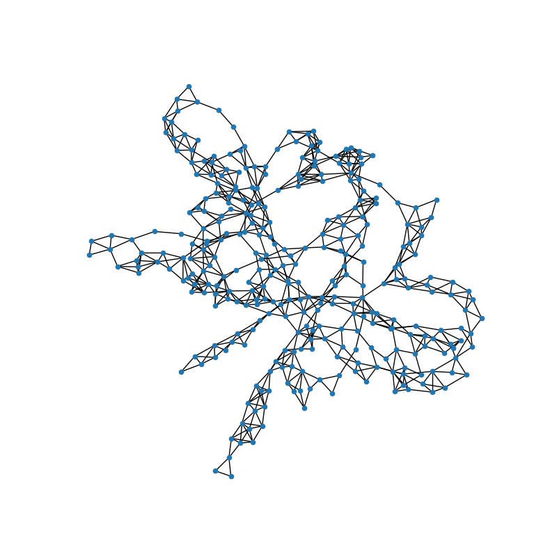
(a) Original
312 nodes, 761 edges

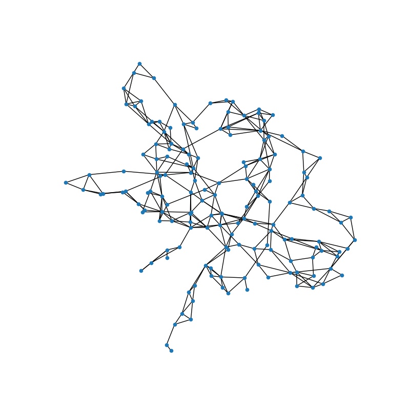
(b) HEM
156 nodes, 340 edges

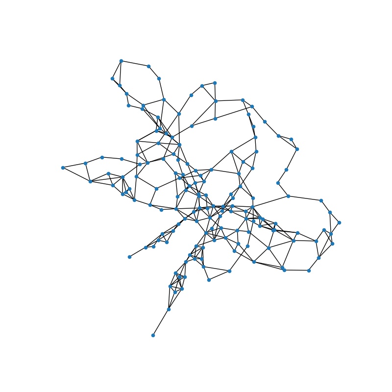
(c) LV
156 nodes, 321 edges

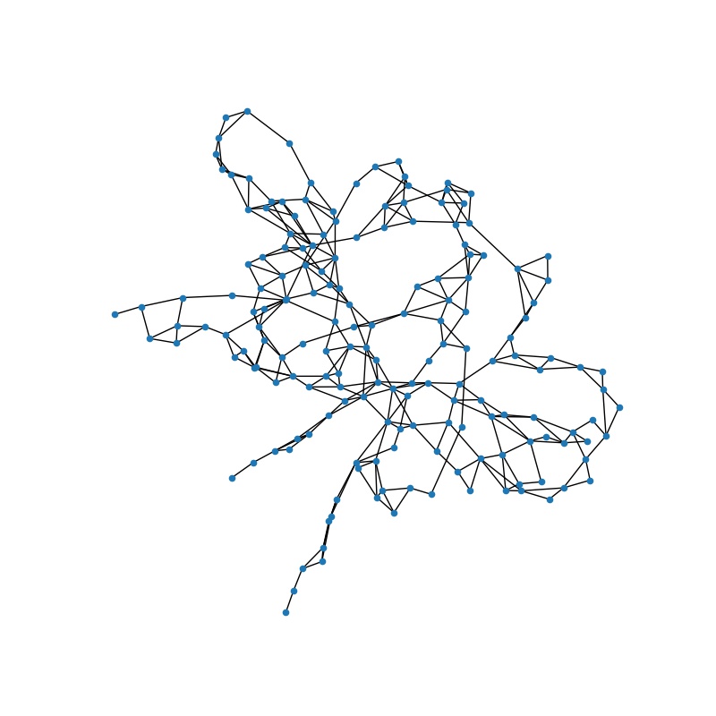
(d) algebraic distance
171 nodes, 327 edges

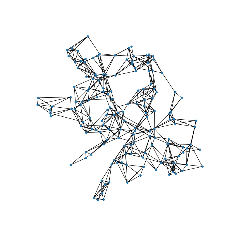
(e) Kron
156 nodes, 485 edges

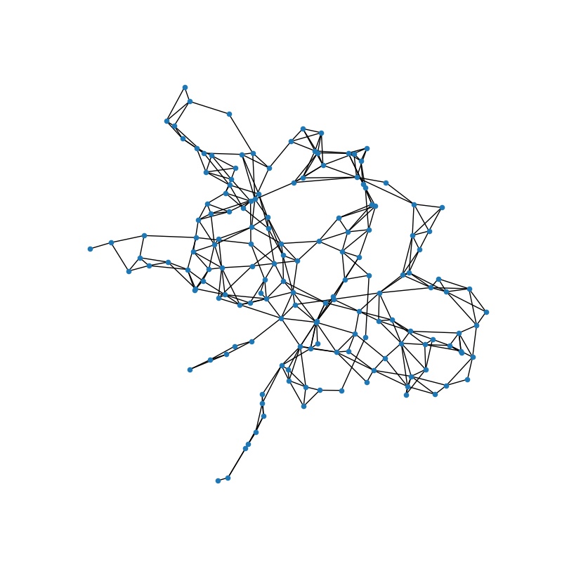
(f) LESC
156 nodes, 362 edges

Figure 9: Visualization of a graph and the coarsened graphs obtained by different methods.

5.3 Interpretations

Leverage scores defined in (30) have been used primarily for matrices that represent data. The form used by us, (31), stabilizes the ordering of the scores when the number $r$ of dominant eigenvectors varies. When $\tau$ or $r$ is large, there is little difference between the value (31) and the following one that uses all eigenvectors:

(32) $$\eta_{i}=\sum_{k=1}^{n}(e^{-\tau\lambda_{k}}U_{ik})^{2}.$$

The form (32) can lead to interesting interpretations and results.

First, observe that if we denote by $e_{i}$ the $i$-th column of the identity matrix, then

(33) $$\eta_{i}=\sum_{k=1}^{n}e^{-2\tau\lambda_{k}}|U_{ik}|^{2}=e_{i}^{T}e^{-2\tau L}e_{i}.$$

That is, $\eta_{i}$ is nothing but the $i$-th diagonal entry of the matrix $H\equiv\exp(-2\tau L)$. If the adjacency matrix $A$ is doubly stochastic, then $L=I-A$ and $H=\exp(-2\tau L)=\exp(-2\tau I+2\tau A)=e^{-2\tau}\times\exp(2\tau A)$. Therefore, since $A$ has nonnegative entries, so does $H$. Then, $H$ is a stochastic matrix (in fact, doubly stochastic because of symmetry). To see this, we have $L\mathbf{1}=0$ and thus by the Taylor series of the matrix exponential, $H\mathbf{1}=\mathbf{1}$. Now that $H$ is a stochastic matrix, the leverage score $\eta_{i}$ ($i$-th diagonal entry of $H$) represents the self-probability of state $i$.

There exists another interpretation from the transient solutions of Markov chains; see Chapter 8 of [113]. In the normalized case, the negative Laplacian $-L$ plays the role of the matrix $Q$ in the notation of continuous time Markov chains (see Section 1.4 of [113]). Given an initial probability distribution $\pi(0)\ \in\ \mathbb{R}^{1\times n}$, the transient solution of the chain at time $t$ is $\pi(t)=\pi(0)\exp(tQ)=\pi(0)\exp(-tL)$. If $\pi(0)=e_{i}^{T}$, then $\pi(t)$ carries the probabilities for each state at time $t$. In particular, the $i$-th entry (which coincides with the leverage score $\eta_{i}$ if $t=2\tau$) is the probability of remaining in state $i$.

5.4 Alternative definition

The definition of $\eta_{i}$ in (31) modifies the standard leverage score by using decaying weights, to reduce sensitivity of the number of eigenvectors used. In principle, any decreasing function of eigenvalues can be used to get distinguishable leverage scores of a Laplacian. We consider the following alternative, which is related to the pseudoinverse of the Laplacian:

(34) $$\eta_{i}=\sum_{j=2}^{n}\left(\frac{1}{\sqrt{\lambda_{j}}}U_{ij}\right)^{2}.$$

Several points are worth noting. First, weighted leverage scores emphasize eigenvectors corresponding to small non-zero eigenvalues. Hence, weighted leverage scores reveal the contribution of nodes to the global structure. Second, a smaller weighted leverage score indicates a higher topological importance of a node. Third, calculating the complete set of eigenvectors of $L$ is expensive. Given a parameter $r$, we can further define $r$-truncated weighted leverage scores using only $r$ eigenpairs:

(35) $$\eta_{i}=\sum_{j=2}^{r}\left(\frac{1}{\sqrt{\lambda_{j}}}U_{ij}\right)^{2}.$$

For simplicity, we refer to these numbers as leverage scores of $L$, and use $\eta=[\eta_{1},\cdots,\eta_{n}]$ to denote them. A visual example of using $\eta$ to define the traversal order in Algorithm 3 is given in Figure 10.

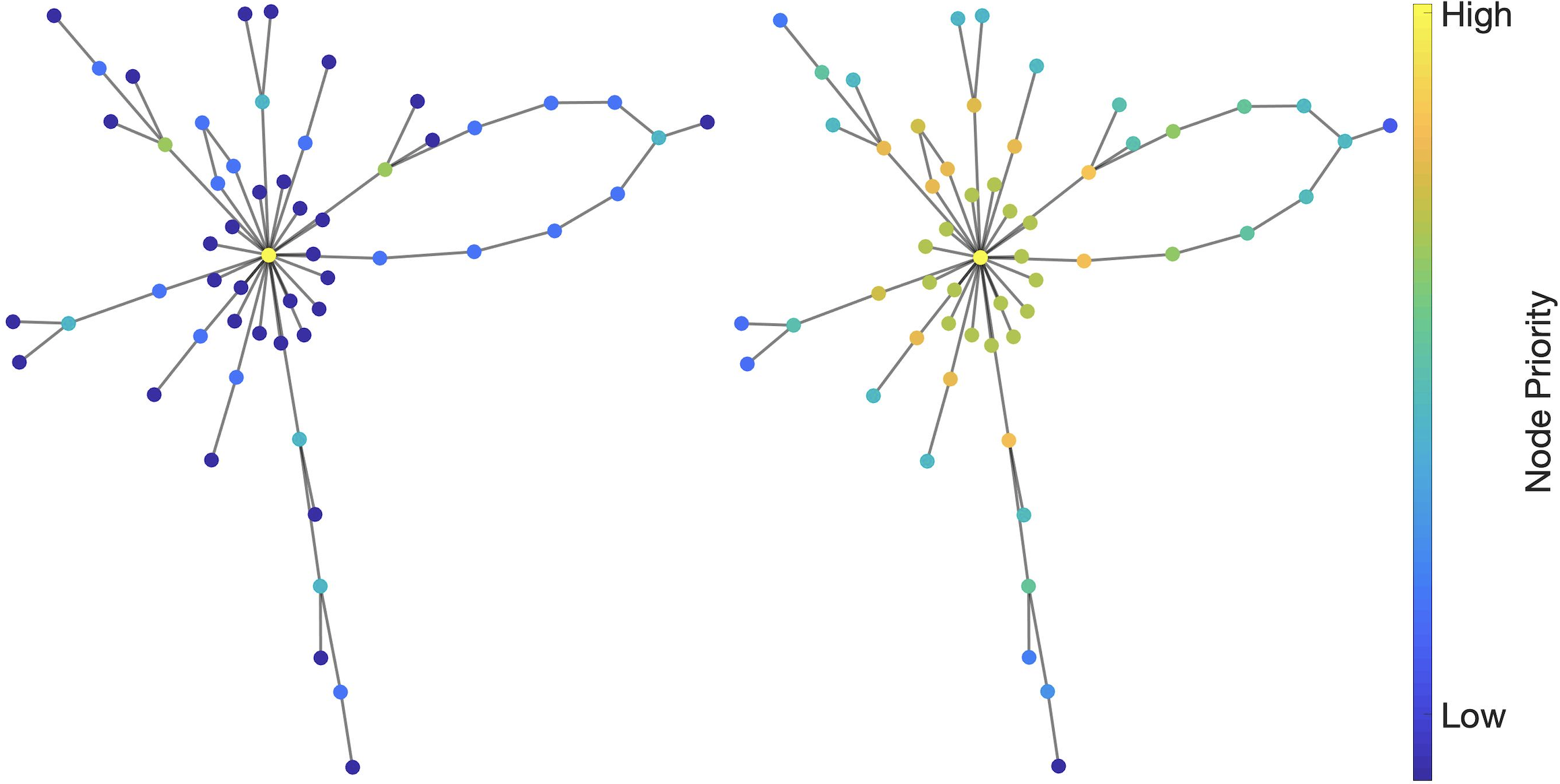
Figure 10: Traversal order of HEM (left) and LESC (right) on an unweighted graph.

The definition (34) has a direct connection with the pseudoinverse of the Laplacian. In particular, the vector $\eta$ is equal to the diagonal of $L^{\dagger}$. To see this, we first notice that $L$ and $L^{\dagger}$ have the same set of eigenvectors, and nontrivial eigenvalues are reciprocals of each other. We then write $L^{\dagger}$ as $L^{\dagger}=U\Sigma^{\dagger}U^{T}$, where $\Sigma^{\dagger}$ is a diagonal matrix with $0<1/\lambda_{n}\leq\cdots\leq 1/\lambda_{2}$ on the diagonal. Diagonal entries of $\Sigma^{\dagger}$ are non-negative, so we can write

(36) $$L^{\dagger}=U\sqrt{\Sigma^{\dagger}}\left(U\sqrt{\Sigma^{\dagger}}\right)^{T},$$

from which we get

$$L_{ii}^{\dagger}=\sum_{j=2}^{n}\frac{U_{ij}}{\sqrt{\lambda_{j}}}\frac{U_{ij}}{\sqrt{\lambda_{j}}}=\eta_{i}.$$

The pseudoinverse of $L$ has long been used to denote node importance. The article [116] provides a rather detailed description of the link between $L^{\dagger}$ and the various definitions of network properties. The effective resistance distance between nodes $a$ and $b$ is given by $\omega_{ab}=L^{\dagger}_{aa}+L^{\dagger}_{bb}-2L^{\dagger}_{ab}$. The trace of $L^{\dagger}$ defines a graph metric called effective graph resistance [49], which is related to random walks [34] and the betweenness centrality [86]. In addition, the columns $s_{j}$ of the matrix $U\sqrt{\Sigma^{\dagger}}$ in (36) have a particular significance. The squared distance between two columns $s_{a}$ and $s_{b}$ is equal to $\omega_{ab}$ and based on this notion of distance, the authors of [96] propose to use $(L_{ii}^{\dagger})^{-1}$ as a measure of the topological centrality of a node $i$. The smaller the distance, the higher its topological centrality. This metric has been used to quantify the roles of nodes in independent networks [107]. Therefore, by using $\eta$, LESC prioritizes nodes with high importance with respect to this metric.

The leverage score vector $\eta$ is also related to the change of the Laplacian pseudoinverse when merging a pair of nodes in coarsening. We follow the work by [61] to elucidate this. To simplify the comparison between two matrices with different sizes, consider the following perspective: during coarsening, instead of merging a pair of nodes and reducing the graph size by one, we assign the corresponding edge with an edge weight $+\infty$. To avoid possible confusion with $L_{c}$, we use $L_{\infty}$ to denote the coarse graph Laplacian (the Laplacian of the $+\infty$-weighted graph). Suppose we assign an edge $e(v_{i},v_{j})$ with the $+\infty$ weight, then the difference between $L$ and $L_{\infty}$ is

(37) $$\Delta L=L_{\infty}-L=wb_{e}b_{e}^{T},\quad(w=+\infty)$$

where $b_{e}$ is defined in (5). Then, the change in $L^{\dagger}$ is given by the Woodbury matrix identity [53]:

(38) $$\Delta L^{\dagger}=-\frac{w}{1+wb_{e}^{T}L^{\dagger}b_{e}}L^{\dagger}b_{e}b_{e}^{T}L^{\dagger}=-\frac{1}{b_{e}^{T}L^{\dagger}b_{e}}L^{\dagger}b_{e}b_{e}^{T}L^{\dagger}.\quad(w=+\infty)$$

Thus, the magnitude of $\Delta L^{\dagger}$ can be defined by the Frobenius norm:

(39) $$||\Delta L^{\dagger}||_{F}^{2}=\frac{b_{e}^{T}L^{\dagger}L^{\dagger}b_{e}}{b_{e}^{T}L^{\dagger}b_{e}}.$$

The following result bounds the magnitude of $\Delta L^{\dagger}$ by using leverage scores.

Proposition 5.1.

Let the graph be connected. The magnitude of the difference between $L^{\dagger}$ and $L_{\infty}^{\dagger}$ caused by assigning the $+\infty$ edge weight to an edge $e(i,j)$ is bounded by

$$||\Delta L^{\dagger}||_{F}^{2}\leq\kappa(L)(L_{ii}^{\dagger}+L_{jj}^{\dagger}),$$

where $\kappa$ denotes the effective condition number (i.e., the largest singular value divided by the smallest nonzero singular value).

Proof 5.2.

Let $L^{\dagger}=U\Lambda U^{T}$ be the spectral decomposition of $L^{\dagger}$ with eigenvalues sorted nonincreasingly: $\mu_{1}\geq\cdots\geq\mu_{n-1}>0=\mu_{n}$. Further, let $x=\Lambda^{1/2}U^{T}b_{e}$. Then,

$$\frac{b_{e}^{T}L^{\dagger}L^{\dagger}b_{e}}{b_{e}^{T}L^{\dagger}b_{e}}=\frac{x^{T}\Lambda x}{x^{T}x}\leq\mu_{1}.$$

Now consider a lower bound and an upper bound of $b_{e}^{T}L^{\dagger}b_{e}$. Since $b_{e}$ is orthogonal to the vector of all ones (an eigenvector associated with $\mu_{n}$), we have

$$\left(\frac{b_{e}}{\sqrt{2}}\right)^{T}L^{\dagger}\left(\frac{b_{e}}{\sqrt{2}}\right)\geq\min_{\|y\|=1}\{y^{T}L^{\dagger}y\mid y^{T}\mathbf{1}=0\}=\mu_{n-1}.$$

On the other hand, note that $b_{e}^{T}L^{\dagger}b_{e}=L^{\dagger}_{ii}+L^{\dagger}_{jj}-2L^{\dagger}_{ij}$ and that $(L^{\dagger}_{ij})^{2}\leq L^{\dagger}_{ii}L^{\dagger}_{jj}$ (by positive semidefiniteness). Then,

$$b_{e}^{T}L^{\dagger}b_{e}\leq\left(\sqrt{L^{\dagger}_{ii}}+\sqrt{L^{\dagger}_{jj}}\right)^{2}\leq 2(L^{\dagger}_{ii}+L^{\dagger}_{jj}).$$

Invoking both the lower bound and the upper bound, we obtain

$$\frac{b_{e}^{T}L^{\dagger}L^{\dagger}b_{e}}{b_{e}^{T}L^{\dagger}b_{e}}\leq\mu_{1}\leq\mu_{1}\frac{2(L^{\dagger}_{ii}+L^{\dagger}_{jj})}{2\mu_{n-1}}.$$

Then, by noting that $\mu_{1}/\mu_{n-1}$ is the effective condition number of $L^{\dagger}$ (as well as $L$), we conclude the proof.

5.5 Experimental results

Here, we show an experiment to demonstrate the effective use of LESC to speed up the training of GNNs. We focus on the task of graph classification that assigns a label to a graph (see Section 3.3). As mentioned in that section, we classify the coarsened graph rather than the original graph. We use four hierarchical GNNs (SortPool [126], DiffPool [125], TopKPool [52, 32], and SAGPool [72]) to perform the task and investigate the change of training time and prediction accuracy under coarsening.

We use three data sets for evaluation: D&D [44], REDDIT-BINARY (REBI), and REDDIT-MULTI-5K (RE5K) [124]. The first is a protein data set and the label categories are protein functions. Each protein is represented by a graph, where nodes represent amino acids and they are connected if the two acids are less than six Angstroms apart. The last two are are social network data sets collected from the online discussion forum Reddit. Each discussion thread is treated as one graph, in which a node represents a user and there is an edge between two nodes if either of the two users respond to each other’s comment. Statistics of the data sets are given in Table 1.

Table 1: Dataset statistics.

	D&D	REBI	RE5K
#graphs	1178	2000	4999
#classes	2	2	5
Avg.#nodes	284.32	429.63	508.52
Avg.#edges	715.66	497.75	594.87

Figure 11 summarizes the time (bars) and accuracy (percentages) results. Each column is for one GNN and each row is for one data set. Inside a panel, three coarsening methods are compared, each using three coarsening levels.

When comparing times, note that applying coarsening to graph classification incurs two costs: the time to perform coarsening (as preprocessing) and the time for training. Therefore, we normalize the overall time by that of training a GNN without using coarsening. Hence, a relative time $<1$ indicates improvement. In fact, the relative time is just the reciprocal of the speedup.

Here are a few observations regarding training times. First, for all three data sets, time reduction is always observed for HEM and LESC. Second, for these two methods, the coarsening time is almost negligible compared with the training time, whereas LV incurs a substantial overhead for coarsening in several cases. In LV, the coarsening time may even dominate the training time (see REBI and RE5K). Discounting coarsening, however, LV produces coarse graphs that lead to reduced training times. Third, in general, the deeper the levels, the more significant is the time reduction. The highest speedup for LESC, which is approximately 30x, occurs for REBI in three levels of coarsening.

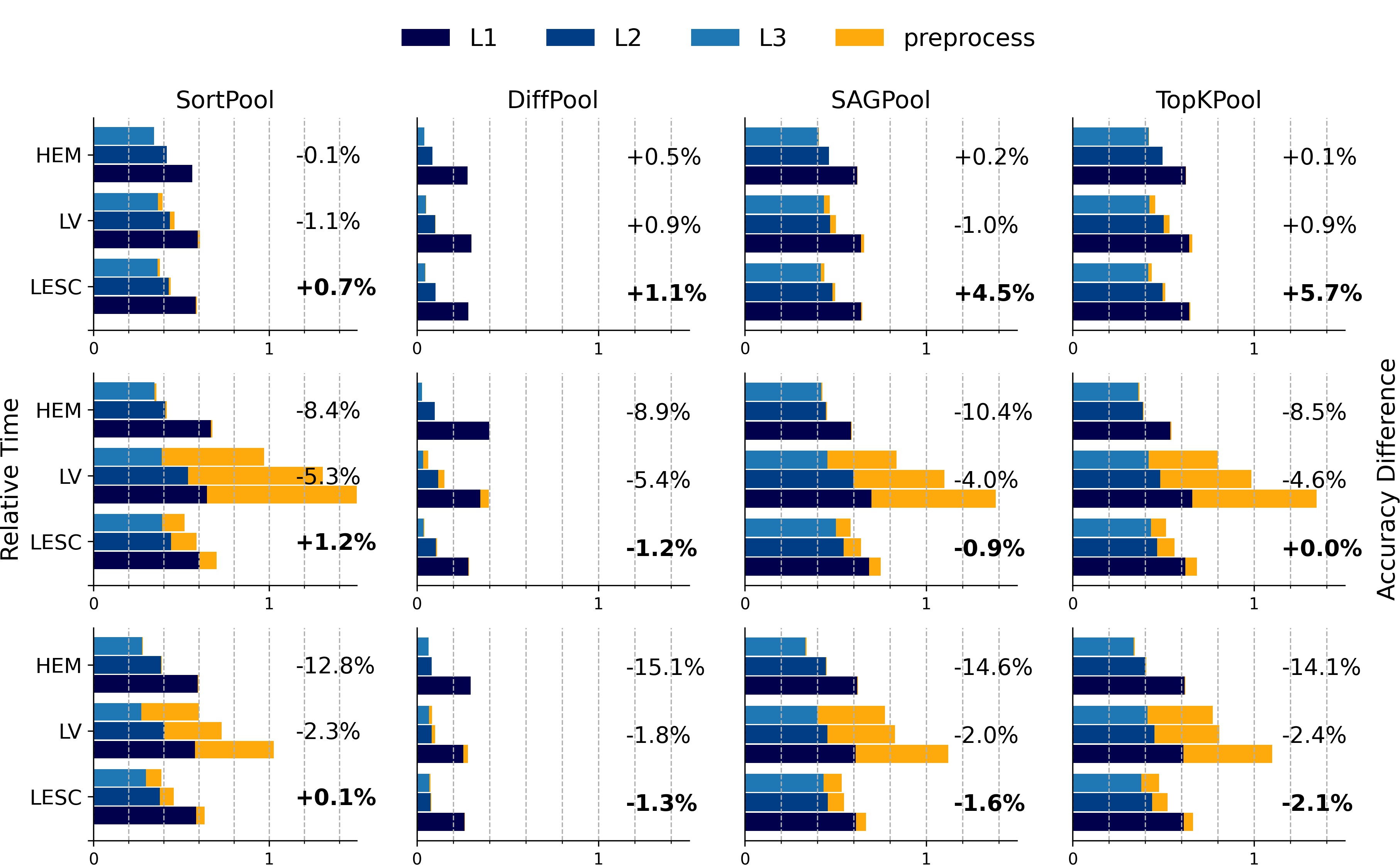
Figure 11: Relative time and accuracy difference on D&D (top row), REBI (middle row), and RE5K (bottom row). Four classification methods (SortPool, DiffPool, SAGPool, and TopKPool) and three coarsening methods (HEM, LV, and LESC) are considered. For each classification method, we normalize the run time by that of the original method. Each run time consists of two parts: coarsening and GNN training with 10-fold cross validation. For each coarsening method, run times are reported for a number of coarsening levels. The highest accuracy achieved by each coarsening method is annotated on the right of the bar chart through differencing from that of the original graph (coarsening minus original). Positive values indicate accuracy increase. The best case for each chart is highlighted in boldface.

To compare prediction accuracies, we compute the relative change (in %) in accuracy and annotate it on the right side of each panel in Figure 11. We see that LESC achieves the best performance among all three coarsening methods on all three datasets. It also improves accuracy on a few of the GNNs while for the others it produces an accuracy that is quite close to that achieved by not using coarsening. In other words, coarsening does not negatively impact graph classification overall.

6 Concluding remarks

This survey (with new results) focused on graph coarsening techniques with a goal of showing how some common ideas have been utilized in two different disciplines while also highlighting methods that are specific to some applications. The recent literature on methods that employ graphs to model data clearly indicates that the general method is likely to gain importance. This is only natural because the graphs encountered today are becoming large and experiments show that if employed with care, coarsening does not cause a big degradation in the performance of the underlying method. As researchers in numerical linear algebra and scientific computing are increasingly turning their attention to problems related to machine learning, graph based methods, and graph coarsening in particular, are likely to play a more prominent role.

References

- [1] A. Ahmed, N. Shervashidze, S. Narayanamurthy, V. Josifovski, and A. J. Smola, Distributed large-scale natural graph factorization, in Proceedings of the 22Nd International Conference on World Wide Web, WWW ’13, New York, NY, USA, 2013, ACM, pp. 37–48.
- [2] I. Althöfer, G. Das, D. Dobkin, D. Joseph, and J. Soares, On sparse spanners of weighted graphs, Discrete & Computational Geometry, 9 (1993), pp. 81–100.
- [3] B. Aspvall and J. R. Gilbert, Graph coloring using eigenvalue decomposition, SIAM Journal on Algebraic Discrete Methods, 5 (1984), pp. 526–538.
- [4] O. Axelsson and M. Larin, An algebraic multilevel iteration method for finite element matrices, J. Comput. Appl. Math., 89 (1997), pp. 135–153.
- [5] O. Axelsson and M. Neytcheva, Algebraic multilevel iteration method for Stieltjes matrices, Numer. Linear Algebra Appl., 1 (1994), pp. 213–236.
- [6] O. Axelsson and B. Polman, A robust preconditioner based on algebraic substructuring and two-level grids, in Robust multigrid methods. Proc., Kiel, Jan. 1988., W. Hackbusch, ed., Notes on Numerical Fluid Mechanics, Volume 23, Vieweg, Braunschweig, 1988, pp. 1–26.
- [7] O. Axelsson and P. Vassilevski, Algebraic multilevel preconditioning methods. I, Numer. Math., 56 (1989), pp. 157–177.
- [8] , A survey of multilevel preconditioned iterative methods, BIT, 29 (1989), pp. 769–793.
- [9] , Algebraic multilevel preconditioning methods. II, SIAM J. Numer. Anal., 27 (1990), pp. 1569–1590.
- [10] N. S. Bakhvalov, On the convergence of a relaxation method with natural constraints on the elliptic operator, U.S.S.R Computational Math. and Math. Phys., 6 (1966), pp. 101–135.
- [11] R. E. Bank and C. Wagner, Multilevel ILU decomposition, Numerische Mathematik, 82 (1999), pp. 543–576.
- [12] S. T. Barnard and H. D. Simon, A fast multilevel implementation of recursive spectral bisection for partitioning unstructured problems, Concurrency: Practice and Experience, 6 (1994), pp. 101–107.
- [13] J. Batson, D. A. Spielman, N. Srivastava, and S.-H. Teng, Spectral sparsification of graphs: Theory and algorithms, Commun. ACM, 56 (2013), p. 87–94.
- [14] M. Belkin and P. Niyogi, Laplacian eigenmaps and spectral techniques for embedding and clustering, in Advances in Neural Information Processing Systems 14, Cambridge, MA, 2002. MIT Press., G. Dietterich, S. Becker, and Z. Ghahramani, eds., 2002.
- [15] M. Belkin and P. Niyogi, Laplacian eigenmaps for dimensionality reduction and data representation, Neural Computation, 15 (2003), pp. 1373–1396.
- [16] A. A. Benczúr and D. R. Karger, Approximating s-t minimum cuts in Õ(n2) time, in Proceedings of the Twenty-Eighth Annual ACM Symposium on Theory of Computing, STOC ’96, New York, NY, USA, 1996, Association for Computing Machinery, p. 47–55.
- [17] M. Benzi, W. Joubert, and G. Mateescu, Numerical experiments with parallel orderings for ILU preconditioners, Electronic Transactions on Numerical Analysis, 8 (1999), pp. 88–114.
- [18] M. Benzi, D. B. Szyld, and A. van Duin, Orderings for incomplete factorizations of nonsymmtric matrices, SIAM Journal on Scientific Computing, 20 (1999), pp. 1652–1670.
- [19] M. Benzi and Tuma, Orderings for factorized sparse approximate inverse preconditioners, SIAM Journal on Scientific Computing, 21 (2000), pp. 1851–1868.
- [20] C. M. Bishop, Pattern Recognition and Machine Learning, Information Science and Statistics, Springer, 2006.
- [21] M. Bollhöfer, A robust ILU with pivoting based on monitoring the growth of the inverse factors, Linear Algebra and its Applications, 338 (2001), pp. 201–213.
- [22] M. Bollhöfer, M. J. Grote, and O. Schenk, Algebraic multilevel preconditioner for the Helmholtz equation in heterogeneous media, SIAM Journal on Scientific Computing, 31 (2009), pp. 3781–3805.
- [23] E. Botta and F. Wubs, Matrix Renumbering ILU: an effective algebraic multilevel ILU, SIAM Journal on Matrix Analysis and Applications, 20 (1999), pp. 1007–1026.
- [24] A. Brandt, Multi-level adaptive solutions to boundary-value problems, Mathematics of Computation, 31 (1977), pp. 333–290.
- [25] , Multiscale scientific computation: review 2001, in Multiscale and multiresolution methods, T. Barth, T. Chan, and R. Haimes, eds., vol. 20 of Lect. Notes Comput. Sci. Eng., Springer-Verlag, 2002, pp. 3–95.
- [26] R. Bridson and W. P. tang, Ordering, anisotropy, and factored sparse approximate inverses, SIAM Journal on Scientific Computing, 21 (1999).
- [27] , A structural diagnosis of some IC orderings, SIAM Journal on Scientific Computing, 22 (2001).
- [28] W. L. Briggs, V. E. Henson, and S. F. Mc Cormick, A multigrid tutorial, SIAM, Philadelphia, PA, 2000. Second edition.
- [29] M. M. Bronstein, J. Bruna, Y. LeCun, A. Szlam, and P. Vandergheynst, Geometric deep learning: Going beyond euclidean data, IEEE Signal Processing Magazine, 34 (2017), pp. 18–42.
- [30] J. Bruna, W. Zaremba, A. Szlam, and Y. LeCun, Spectral networks and locally connected networks on graphs, 2013.
- [31] P. J. Burt and E. H. Adelson, The Laplacian pyramid as a compact image code, in Readings in Computer Vision, M. A. Fischler and O. Firschein, eds., Morgan Kaufmann, San Francisco (CA), 1987, pp. 671–679.
- [32] C. Cangea, P. Velickovic, N. Jovanovic, T. Kipf, and P. Liò, Towards sparse hierarchical graph classifiers, ArXiv, abs/1811.01287 (2018).
- [33] S. Cao, W. Lu, and Q. Xu, Grarep: Learning graph representations with global structural information, in Proceedings of the 24th ACM International on Conference on Information and Knowledge Management, CIKM ’15, New York, NY, USA, 2015, ACM, pp. 891–900.
- [34] A. K. Chandra, P. Raghavan, W. L. Ruzzo, R. Smolensky, and P. Tiwari, The electrical resistance of a graph captures its commute and cover times, Computational Complexity, 6 (1996), pp. 312–340.
- [35] H. Chen, B. Perozzi, Y. Hu, and S. Skiena, HARP: Hierarchical representation learning for networks, Proceedings of the AAAI Conference on Artificial Intelligence, 32 (2018).
- [36] J. Chen and I. Safro, Algebraic distance on graphs, SIAM J. Sci. Comput., 33 (2011), p. 3468–3490.
- [37] K. Chen, Matrix Preconditioning Techniques and Applications, Cambridge University Press, Cambridge, UK,, 2005.
- [38] E. Chow and Y. Saad, Experimental study of ILU preconditioners for indefinite matrices, Journal of Computational and Applied Mathematics, 86 (1997), pp. 387–414.
- [39] S. Clift and W. Tang, Weighted graph based ordering techniques for preconditioned conjugate gradient methods, BIT, 35 (1995), pp. 30–47.
- [40] E. D’Azevedo, P. Forsyth, and W. Tang, Ordering methods for preconditioned conjugate gradient methods applied to unstructured grid problems, SIAM J. Matrix Anal. Applic., 13 (1992), pp. 944–961.
- [41] M. Defferrard, X. Bresson, and P. Vandergheynst, Convolutional neural networks on graphs with fast localized spectral filtering, in Proceedings of the 30th International Conference on Neural Information Processing Systems, NIPS’16, Red Hook, NY, USA, 2016, Curran Associates Inc., p. 3844–3852.
- [42] C. Deng, Z. Zhao, Y. Wang, Z. Zhang, and Z. Feng, Graphzoom: A multi-level spectral approach for accurate and scalable graph embedding, in International Conference on Learning Representations, 2020.
- [43] I. S. Dhillon, Y. Guan, and B. Kulis, Weighted graph cuts without eigenvectors a multilevel approach, IEEE Transactions on Pattern Analysis and Machine Intelligence, 29 (2007), pp. 1944–1957.
- [44] P. D. Dobson and A. J. Doig, Distinguishing enzyme structures from non-enzymes without alignments, Journal of Molecular Biology, 330 (2003), pp. 771–783.
- [45] S. Doi and A. Lichnewsky, A graph theory approach for analyzing the effects of ordering on ILU preconditioning, Tech. Rep. 1452, INRIA, Rocquencourt, France, 1991.
- [46] F. Dorfler and F. Bullo, Kron reduction of graphs with applications to electrical networks, IEEE Transactions on Circuits and Systems I: Regular Papers, 60 (2013), pp. 150–163.
- [47] P. Drineas, M. Magdon-Ismail, M. W. Mahoney, and D. P. Woodruff, Fast approximation of matrix coherence and statistical leverage, J. Mach. Learn. Res., 13 (2012), p. 3475–3506.
- [48] D. K. Duvenaud, D. Maclaurin, J. Iparraguirre, R. Bombarell, T. Hirzel, A. Aspuru-Guzik, and R. P. Adams, Convolutional networks on graphs for learning molecular fingerprints, in Advances in neural information processing systems, 2015, pp. 2224–2232.
- [49] W. Ellens, F. Spieksma, P. Van Mieghem, A. Jamakovic, and R. Kooij, Effective graph resistance, Linear algebra and its applications, 435 (2011), pp. 2491–2506.
- [50] W. Fan, J. Li, X. Wang, and Y. Wu, Query preserving graph compression, in Proceedings of the 2012 ACM SIGMOD International Conference on Management of Data, 2012, pp. 157–168.
- [51] M. Fiedler, Algebraic connectivity of graphs, Czechoslovak Mathematical Journal, 23 (1973), pp. 298–305.
- [52] H. Gao and S. Ji, Graph u-nets, in ICML, 2019.
- [53] D. Goldfarb, Modification methods for inverting matrices and solving systems of linear algebraic equations, Mathematics of Computation, 26 (1972), pp. 829–852.
- [54] G. H. Golub and C. F. V. Loan, Matrix Computations, 4th edition, Johns Hopkins University Press, Baltimore, MD, 4th ed., 2013.
- [55] P. Goyal and E. Ferrara, Graph embedding techniques, applications, and performance: A survey, Knowledge-Based Systems, 151 (2018), pp. 78–94.
- [56] A. Grover and J. Leskovec, Node2vec: Scalable feature learning for networks, in Proceedings of the 22Nd ACM SIGKDD International Conference on Knowledge Discovery and Data Mining, KDD ’16, New York, NY, USA, 2016, ACM, pp. 855–864.
- [57] W. Hackbusch, Multi-Grid Methods and Applications, vol. 4 of Springer Series in Computational Mathematics, Springer-Verlag, Berlin, 1985.
- [58] W. Hamilton, Z. Ying, and J. Leskovec, Inductive representation learning on large graphs, in Advances in neural information processing systems, 2017, pp. 1024–1034.
- [59] W. L. Hamilton, R. Ying, and J. Leskovec, Representation learning on graphs: Methods and applications, 2017.
- [60] M. Henaff, J. Bruna, and Y. LeCun, Deep convolutional networks on graph-structured data, 2015.
- [61] G. B. Hermsdorff and L. Gunderson, A unifying framework for spectrum-preserving graph sparsification and coarsening, in Advances in Neural Information Processing Systems, 2019, pp. 7736–7747.
- [62] Y. F. Hu and R. J. Blake, Load balancing for unstructured mesh applications, Nova Science Publishers, Inc., Commack, NY, USA, 2001, pp. 117–148.
- [63] Y. Jin, A. Loukas, and J. JaJa, Graph coarsening with preserved spectral properties, in International Conference on Artificial Intelligence and Statistics, PMLR, 2020, pp. 4452–4462.
- [64] M. Kapralov, Y. T. Lee, C. Musco, C. Musco, and A. Sidford, Single pass spectral sparsification in dynamic streams, in Foundations of Computer Science (FOCS), 2014 IEEE 55th Annual Symposium on, IEEE, 2014, pp. 561–570.
- [65] D. R. Karger, Random sampling in cut, flow, and network design problems, in Proceedings of the Twenty-Sixth Annual ACM Symposium on Theory of Computing, STOC ’94, New York, NY, USA, 1994, Association for Computing Machinery, p. 648–657.
- [66] G. Karypis and V. Kumar, Multilevel graph partitioning schemes, in Proc. 24th Intern. Conf. Par. Proc., III, CRC Press, 1995, pp. 113–122.
- [67] B. W. Kernighan and S. Lin, An efficient heuristic procedure for partitioning graphs, The Bell System Technical Journal, 29 (1970), pp. 291–307.
- [68] T. N. Kipf and M. Welling, Semi-supervised classification with graph convolutional networks, 2016.
- [69] B. Knyazev, G. W. Taylor, and M. R. Amer, Understanding attention and generalization in graph neural networks, 2019.
- [70] R. Krauthgamer, Sketching graphs and combinatorial optimization (invited talk), in 47th International Colloquium on Automata, Languages, and Programming (ICALP 2020), Schloss Dagstuhl-Leibniz-Zentrum für Informatik, 2020.
- [71] G. Kron, Tensor Analysis of Networks, Wiley, New York, 1939.
- [72] J. Lee, I. Lee, and J. Kang, Self-attention graph pooling, in ICML, 2019.
- [73] J. Liang, S. Gurukar, and S. Parthasarathy, MILE: a multi-level framework for scalable graph embedding, ArXiv preprint arXiv:1802.09612 [cs.AI], (2018).
- [74] Y. Liu, T. Safavi, A. Dighe, and D. Koutra, Graph summarization methods and applications: A survey, ACM Computing Surveys (CSUR), 51 (2018), pp. 1–34.
- [75] A. Loukas, Graph reduction with spectral and cut guarantees, Journal of Machine Learning Research, 20 (2019), pp. 1–42.
- [76] T. Ma and J. Chen, Unsupervised learning of graph hierarchical abstractions with differentiable coarsening and optimal transport, in Proceedings of the Thirty-Fifth AAAI Conference on Artificial Intelligence, 2021.
- [77] S. MacLachlan, D. Osei-Kuffuor, and Y. Saad, Modification and compensation strategies for threshold-based incomplete factorizations, SIAM Journal on Scientific Computing, 34 (2012), pp. A48–A75.
- [78] S. MacLachlan and Y. Saad, Greedy coarsening strategies for non-symmetric problems, SIAM Journal on Scientific Computing, 29 (2007), pp. 2115–2143.
- [79] , A greedy strategy for coarse-grid selection, SIAM Journal on Scientific Computing, 29 (2007), pp. 1825–1853.
- [80] R. M. Martin, Electronic Structure, basic theory and practical methods, Cambridge University Press, Cambridge, UK, 2004.
- [81] J. Mayer, A multilevel Crout ILU preconditioner with pivoting and row permutation, Numerical Linear Algebra with Applications, 14 (2007), pp. 771–789.
- [82] F. Monti, D. Boscaini, J. Masci, E. Rodola, J. Svoboda, and M. M. Bronstein, Geometric deep learning on graphs and manifolds using mixture model cnns, in The IEEE Conference on Computer Vision and Pattern Recognition (CVPR), July 2017.
- [83] C. Morris, M. Ritzert, M. Fey, W. L. Hamilton, J. E. Lenssen, G. Rattan, and M. Grohe, Weisfeiler and leman go neural: Higher-order graph neural networks., in AAAI, 2019, pp. 4602–4609.
- [84] A. C. Muresan and Y. Notay, Analysis of aggregation-based multigrid, SIAM Journal on Scientific Computing, 30 (2008), pp. 1082–1103.
- [85] S. Navlakha, R. Rastogi, and N. Shrivastava, Graph summarization with bounded error, in Proceedings of the 2008 ACM SIGMOD international conference on Management of data, 2008, pp. 419–432.
- [86] M. E. Newman, A measure of betweenness centrality based on random walks, Social networks, 27 (2005), pp. 39–54.
- [87] M. Niepert, M. Ahmed, and K. Kutzkov, Learning convolutional neural networks for graphs, in Proceedings of the 33rd International Conference on International Conference on Machine Learning - Volume 48, ICML’16, JMLR.org, 2016, p. 2014–2023.
- [88] Y. Notay, An aggregation-based algebraic multigrid method, Electronic Transactions on Numerical Analysis, 37 (2010), pp. 123–146.
- [89] D. Osei-Kuffuor, R. Li, and Y. Saad, Matrix reordering using multilevel graph coarsening for ILU preconditioning, SIAM Journal on Scientific Computing, 37 (2015), pp. A391–A419.
- [90] B. Perozzi, R. Al-Rfou, and S. Skiena, Deepwalk: Online learning of social representations, in Proceedings of the 20th ACM SIGKDD international conference on Knowledge discovery and data mining, 2014, pp. 701–710.
- [91] A. Pothen, H. Simon, and K.-P. Liou, Partitioning sparse matrices with eigenvectors of graphs, SIAM Journal on Matrix Analysis and Applications, 11 (1990), pp. 430–452.
- [92] D. Powers, Evaluation: From precision, recall and f-factor to roc, informedness, markedness & correlation, Mach. Learn. Technol., 2 (2008).
- [93] B. Quiring and P. S. Vassilevski, Multilevel graph embedding, Numerical Linear Algebra with Applications, 28 (2021), p. e2326.
- [94] H. r. Fang and Y. Saad, Hypergraph-based multilevel matrix approximation for text information retrieval, in Proceedings of the ACM International Conference on Information and Knowledge Management, 2010, J. H. et al., ed., 2010, pp. 1597–1600.
- [95] H. r. Fang, S. Sakellaridi, and Y. Saad, Multilevel manifold learning with application to spectral clustering, in Proceedings of the ACM International Conference on Information and Knowledge Management, 2010, J. H. et al., ed., 2010, pp. 419–428.
- [96] G. Ranjan and Z.-L. Zhang, Geometry of complex networks and topological centrality, Physica A: Statistical Mechanics and its Applications, 392 (2013), pp. 3833–3845.
- [97] D. Ron, I. Safro, and A. Brandt, Relaxation-based coarsening and multiscale graph organization, SIAM Multiscale Modelling and Simulations, 9 (2011), pp. 407–423.
- [98] R. Roth, On the eigenvectors belonging to the minimum eigenvalue of an essentially nonnegative symmetric matrix with bipartite graph, Linear Algebra and its Applications, 118 (1989), pp. 1–10.
- [99] S. Roweis and L. Saul, Nonlinear dimensionality reduction by locally linear embedding, Science, 290 (2000), pp. 2323–2326.
- [100] A. Ruge and K. Stüben, Algebraic multigrid, in Multigrid Methods, S. McCormick, ed., vol. 3 of Frontiers in Applied Mathematics, SIAM, 1987, ch. 4, pp. 73–130.
- [101] Y. Saad, Iterative Methods for Sparse Linear Systems, 2nd edition, SIAM, Philadelpha, PA, 2003.
- [102] , Multilevel ILU with reorderings for diagonal dominance, SIAM Journal on Scientific Computing, 27 (2005), pp. 1032–1057.
- [103] Y. Saad, Numerical Methods for Large Eigenvalue Problems-classics edition, SIAM, Philadelphia, 2011.
- [104] Y. Saad and B. Suchomel, ARMS: An algebraic recursive multilevel solver for general sparse linear systems, Numerical Linear Algebra with Applications, 9 (2002).
- [105] S. Sakellaridi, H. R. Fang, and Y. Saad, Graph-based multilevel dimensionality reduction with applications to eigenfaces and latent semantic indexing, in Proceedings of Int. Conf. Mach. Learn. Appls. (ICMLA), 2008, M. A. Wani, ed., IEEE comp. Soc., 2008, pp. 194–200.
- [106] P. Sen, G. Namata, M. Bilgic, L. Getoor, B. Galligher, and T. Eliassi-Rad, Collective classification in network data, AI magazine, 29 (2008), pp. 93–93.
- [107] D.-H. Shin, D. Qian, and J. Zhang, Cascading effects in interdependent networks, IEEE Network, 28 (2014), pp. 82–87.
- [108] D. I. Shuman, M. J. Faraji, and P. Vandergheynst, A multiscale pyramid transform for graph signals, IEEE Transactions on Signal Processing, 64 (2016), pp. 2119–2134.
- [109] D. I. Shuman, S. K. Narang, P. Frossard, A. Ortega, and P. Vandergheynst, The emerging field of signal processing on graphs: Extending high-dimensional data analysis to networks and other irregular domains, IEEE Signal Processing Magazine, 30 (2013), pp. 83–98.
- [110] M. Simonovsky and N. Komodakis, Dynamic edge-conditioned filters in convolutional neural networks on graphs, in Proceedings of the IEEE conference on computer vision and pattern recognition, 2017, pp. 3693–3702.
- [111] D. A. Spielman and N. Srivastava, Graph sparsification by effective resistances, SIAM Journal on Computing, 40 (2011), pp. 1913–1926.
- [112] D. A. Spielman and S.-H. Teng, Spectral sparsification of graphs, SIAM Journal on Computing, 40 (2011), pp. 981–1025.
- [113] W. J. Stewart, Introduction to the Numerical Solution of Markov Chains, Princeton University Press, Princeton, NJ, 1994.
- [114] J. Tang, M. Qu, M. Wang, M. Zhang, J. Yan, and Q. Mei, Line: Large-scale information network embedding, in Proceedings of the 24th International Conference on World Wide Web, WWW ’15, Republic and Canton of Geneva, CHE, 2015, International World Wide Web Conferences Steering Committee, p. 1067–1077.
- [115] U. Trottenberg, C. Oosterlee, and A. Schüller, Multigrid, Academic Press, San Diego, CA, 2001.
- [116] P. Van Mieghem, K. Devriendt, and H. Cetinay, Pseudoinverse of the Laplacian and best spreader node in a network, Physical Review E, 96 (2017), p. 032311.
- [117] N. Vannieuwenhoven and K. Meerbergen, IMF: An incomplete multifrontal LU-factorization for element-structured sparse linear systems, SIAM Journal on Scientific Computing, 35 (2013), pp. A270–A293.
- [118] P. Vaněk, M. Brezina, and J. Mandel, Convergence of algebraic multigrid based on smoothed aggregation, Numerische Mathematik, 88 (2001), pp. 559–579.
- [119] P. Vaněk, J. Mandel, and M. Brezina, Algebraic multigrid by smoothed aggregation for second and fourth order elliptic problems, Computing, 56 (1996), pp. 179–196.
- [120] P. Veličković, G. Cucurull, A. Casanova, A. Romero, P. Liò, and Y. Bengio, Graph attention networks, 2017.
- [121] N. Wale and G. Karypis, Comparison of descriptor spaces for chemical compound retrieval and classification, in Sixth International Conference on Data Mining (ICDM’06), Dec 2006, pp. 678–689.
- [122] X. Wang, P. Cui, J. Wang, J. Pei, W. Zhu, and S. Yang, Community preserving network embedding, in Proceedings of the Thirty-First AAAI Conference on Artificial Intelligence (AAAI-17), 2017, pp. 203–209.
- [123] K. Xu, W. Hu, J. Leskovec, and S. Jegelka, How powerful are graph neural networks?, 2018.
- [124] P. Yanardag and S. Vishwanathan, Deep graph kernels, in Proceedings of the 21th ACM SIGKDD International Conference on Knowledge Discovery and Data Mining, KDD ’15, New York, NY, USA, 2015, Association for Computing Machinery, p. 1365–1374.
- [125] R. Ying, J. You, C. Morris, X. Ren, W. L. Hamilton, and J. Leskovec, Hierarchical graph representation learning with differentiable pooling, in Proceedings of the 32Nd International Conference on Neural Information Processing Systems, NIPS’18, USA, 2018, Curran Associates Inc., pp. 4805–4815.
- [126] M. Zhang, Z. Cui, M. Neumann, and Y. Chen, An end-to-end deep learning architecture for graph classification, in AAAI, 2018.