HybVIO: Pushing the Limits of Real-time Visual-inertial Odometry

Abstract

We present HybVIO, a novel hybrid approach for combining filtering-based visual-inertial odometry (VIO) with optimization-based SLAM. The core of our method is highly robust, independent VIO with improved IMU bias modeling, outlier rejection, stationarity detection, and feature track selection, which is adjustable to run on embedded hardware. Long-term consistency is achieved with a loosely-coupled SLAM module. In academic benchmarks, our solution yields excellent performance in all categories, especially in the real-time use case, where we outperform the current state-of-the-art. We also demonstrate the feasibility of VIO for vehicular tracking on consumer-grade hardware using a custom dataset, and show good performance in comparison to current commercial VISLAM alternatives.

1 Introduction

Visual-inertial odometry (VIO) refers to the tracking of the position and orientation of a device using one or more cameras and an inertial measurement unit (IMU), which, in this context, is assumed to comprise of at least an accelerometer and a gyroscope. A closely related term is visual-inertial SLAM (VISLAM), which is typically used to describe methods that possess a longer memory than VIO: simultaneously with tracking, they produce a map of the environment, which can be used to correct accumulated drift in the case the device revisits a previously mapped area. Without additional inputs, these methods can only estimate the location relative to the starting point but provide no global position information. In the visual–inertial context, the orientation of the device also has one unsolvable degree of freedom: the rotation about the gravity axis, or equivalently, the initial compass heading of the device.

VISLAM is the basic building block of infrastructure-free augmented reality applications. VIO, especially when fused with satellite navigation (GNSS), can be applied to tracking of various types of both industrial and personal vehicles, where it can maintain accurate tracking during GNSS outages, for instance, in highway tunnels. One of the main advantages of VIO over pure inertial navigation (INS), and consequently, the advantage of GNSS-VIO over GNSS-INS, is improved long-range accuracy. VIO can provide similar accuracy with consumer-grade hardware, than INS with high-end IMUs that are prohibitively expensive for any consumer applications.

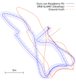
Figure 1: Real-time VIO with uncertainty quantification on an embedded processor compared to ORB-SLAM3 on a desktop CPU. The latter remains the leader in the EuRoC post-processing category, while our method yields the best online results.

The contributions of this paper are as follows. (i) We extend the probabilistic inertial-visual odometry (PIVO) methodology from monocular-only to stereo. (ii) We improve the IMU bias modeling in PIVO with Ornstein-Uhlenbeck random walk processes. (iii) We derive improved mechanisms for outlier detection, stationarity detection, and feature track selection that leverage the unique features of the probabilistic framework. (iv) We present a novel hybrid method for ego-motion estimation, where extended Kalman filtering based VIO is combined with optimization-based SLAM.

These methods enable state-of-the-art performance in various use cases (online, offline, monocular, and stereo). In particular, we outperform the previous leader, BASALT, in EuRoC MAV. We also demonstrate the vehicular tracking capabilities of our VIO module with consumer-grade hardware, as well as our accuracy compared to commercial alternatives, using a custom dataset.

2 Related work

Our VIO module is a stereoscopic extension of PIVO [34] and, consequently, a member of the MSCKF family of VIO methods that stems from [18]. Other recent methods belonging to the same class include the hybrid-EKF-SLAM (cf. [16]) method LARVIO [26] and S-MSCKF [37], which extends the original MSCKF to stereo cameras. These methods, following their EKF-SLAM predecessors (e.g., [8]), use an Extended Kalman Filter (EKF) to keep track of the VIO state. They track the Bayesian conditional mean (CM) of the VIO state and keep it in memory together with its full covariance matrix, which limits the practical dimension of the state vector in real-time use cases.

An alternative to the above filtering-based methods are optimization-based approaches, which compute a Maximum A Posteriori (MAP) estimate in place of the conditional mean, and instead of storing a full covariance matrix, they may use sparse Bayesian factor graphs. The optimization-based methods are often stated to be more accurate than filtering-based methods and many recent publications prefer this approach. Notable examples include OKVIS [15], MARS-VINS [23], ORB-SLAM3 [5], BASALT [41] and Kimera-VIO [28].

However, there are also disadvantages compared to filtering-based methods, namely, the lack of uncertainty quantification capabilities and the difficulty of marginalizing the active state on all the past data. Our method includes elements from both approaches, as filtering-based VIO is loosely coupled with optimization-based SLAM module. Previously, good results for post-processed trajectories have been reported with hybrid filtering–optimization approaches in, e.g., [27] and [1]. However, our approach differs from these tightly-coupled solutions. In addition to the more common sparse approaches above, various alternatives have been proposed (see, e.g., [2, 7, 9, 38, 42]). For a more extensive survey of recent and historical methods, we refer the reader to [5] and the references therein.

3 Method description

3.1 VIO state definition

Similarly to [34] and [18], we construct the VIO state vector at time step $t_{k}$,

$$\mathbf{x}_{k}=(\bm{\pi}^{(0)}_{k},\mathbf{v}_{k},\mathbf{b}_{k},\tau_{k},\bm{\pi}^{(1)}_{k},\ldots,\bm{\pi}^{(n_{a})}_{k}),$$ (1)

using the poses $\bm{\pi}^{(j)}_{k}=(\mathbf{p}^{(j)}_{k},\mathbf{q}^{(j)}_{k})\in\mathbb{R}^{3}\times\mathbb{R}^{4}$ of the IMU sensor at the latest input sample ($j=0$) and a fixed-size window of recent camera frames ($j=1,\ldots,n_{a}$). The other elements in Eq. 1 are the current velocity $\mathbf{v}_{k}\in\mathbb{R}^{3}$, a vector of IMU biases $\mathbf{b}_{k}=(\mathbf{b}^{\rm a}_{k},\mathbf{b}^{\omega}_{k},\operatorname{diag}(\mathbf{T}^{\rm a}_{k}))$ (see Eq. 3), and an IMU-camera time shift parameter $\tau_{k}\in\mathbb{R}$, utilized as described in [25].

In the EKF framework, the probability distribution of the state, given all the observations $\mathbf{y}_{1:k}$ until time $t_{k}$, is modeled as Gaussian, $\mathbf{x}_{k}|\mathbf{y}_{1:k}\sim\mathcal{N}(\mathbf{m}_{k|k},\mathbf{P}_{k|k})$. We model the orientation quaternions as Gaussians in $\mathbb{R}^{4}$ and restore their unit length after each EKF update step.

3.2 IMU propagation model

The VIO system is initialized to $(\mathbf{m}_{1|1},\mathbf{P}_{1|1})$, where the current orientation $\mathbf{q}^{(0)}_{1|1}$ is based on the first IMU samples equally to [35]. The other components of $\mathbf{m}_{1|1}$ are fixed (zero or one), and $\mathbf{P}_{1|1}$ is a fixed diagonal matrix. No other measures are required to initialize the system.

Following [34], IMU propagation is performed on each synchronized pair $(\bm{\omega}_{k},\mathbf{a}_{k})$ of gyroscope and accelerometer samples as an EKF prediction step of the form

$$\mathbf{x}_{k|k-1}=\mathbf{f}_{k}(\mathbf{x}_{k-1|k-1},\bm{\varepsilon}_{k})$$ (2)

with $\bm{\varepsilon}_{k}\sim\mathcal{N}(\mathbf{0},\mathbf{Q}\Delta t_{k})$. The function $\mathbf{f}_{k}$ updates the pose and velocity by the mechanization equation

$$\begin{pmatrix}\mathbf{p}_{k}\\ \mathbf{v}_{k}\\ \mathbf{q}_{k}\end{pmatrix}=\begin{pmatrix}\mathbf{p}_{k-1}+\mathbf{v}_{k-1}\Delta t_{k}\\ \mathbf{v}_{k-1}+[\mathbf{q}_{k}(\tilde{\mathbf{a}}_{k}+\bm{\varepsilon}^{\mathrm{a}}_{k})\mathbf{q}_{k}^{\star}-\mathbf{g}]\Delta t_{k}\\ \bm{\Omega}[(\tilde{\bm{\omega}}_{k}+\bm{\varepsilon}^{\omega}_{k})\Delta t_{k}]\mathbf{q}_{k-1}\end{pmatrix},$$ (3)

where the bias-corrected IMU measurements are computed as $\tilde{\mathbf{a}}_{k}=\mathbf{T}_{k}^{\mathrm{a}}\,\mathbf{a}_{k}-\mathbf{b}^{\mathrm{a}}_{k}$ and $\tilde{\bm{\omega}}_{k}=\bm{\omega}_{k}-\mathbf{b}^{\omega}_{k}$. In our model, the multiplicative correction $\mathbf{T}_{k}^{\mathrm{a}}\in\mathbb{R}^{3\times 3}$ is a diagonal matrix.

Contrary to the approach used in [18], this does not involve linearization errors that could cause the orientation quaternion to lose its unit length, since $\bm{\Omega}[\cdot]\in\mathbb{R}^{4\times 4}$ (cf. [39] or Eq. A3) is an orthogonal matrix.

As an extension to [34], we assume the following model for the IMU biases:

$$\begin{pmatrix}\mathbf{b}^{\mathrm{a}}_{k}\\ \mathbf{b}^{\omega}_{k}\\ \mathbf{T}_{k}^{\mathrm{a}}\end{pmatrix}=\begin{pmatrix}\exp(-\alpha_{\rm a}\Delta t_{k})\mathbf{b}^{\mathrm{a}}_{k-1}+\epsilon_{k}^{\rm a}\\ \exp(-\alpha_{\omega}\Delta t_{k})\mathbf{b}^{\omega}_{k-1}+\epsilon_{k}^{\omega}\\ \mathbf{T}_{k-1}^{\mathrm{a}}\end{pmatrix},$$ (4)

where the parameters $\alpha,\sigma$ in the Ornstein–Uhlenbeck [40] random walks $\epsilon_{k}\sim\mathcal{N}(\mathbf{0},\frac{\sigma^{2}}{2\alpha}[1-\exp(-2\alpha\Delta t_{k})])$ can be adjusted to match the characteristics of the IMU sensor.

3.3 Feature tracking

Similarly to [18], our visual updates are based on the constraints induced by viewing certain point features from multiple camera frames. We first utilize the Good Features to Track (GFTT) algorithm [33] (or, alternatively, FAST [29], cf. Table 1) for detecting an initial set of features, which are subsequently tracked between consecutive frames using the pyramidal Lucas–Kanade method [17] as implemented in the OpenCV library [3]. We also use the reprojections of previously triangulated 3D positions (cf. Sec. 3.6) of the features as initial values for the LK tracker whenever available, which improves its accuracy and robustness, especially during rapid camera movements.

As in [34], features lost due to falling out of the view of the camera, or any other reason, are replaced by detecting new key points whenever the number of tracked features falls below a certain threshold. A minimum distance between features is also imposed in the detection phase and sub-pixel adjustment is performed on the new features.

In the case of stereo data, we detect the new features in the left camera frame, and find the matching points in the right camera frame, also using the Lucas–Kanade algorithm. This technique allows the use of raw camera images without a separate stereo rectification phase. The temporal tracking is only performed on the left camera frames, and the matches in the right frame are recomputed on each image. In addition, we reject features with incorrect stereo matches based on an epipolar constraint check.

Unlike [34], we additionally utilize a 3-point stereo RANSAC method described in [22] or, in the monocular case, a mixture of 2-point (rotation only, cf. [13]) and 5-point RANSAC methods [21], for rejecting outlier features.

3.4 Visual update track selection

A feature track $\mathbf{y}^{j}$ with index $j\in\mathbb{N}$ is, in the monocular case, a list of pixel coordinates ($\mathbf{y}^{j}_{i}\in\mathbb{R}^{2}$), or pairs of coordinates $\mathbf{y}^{j,R}_{i},\mathbf{y}^{j,L}_{i}\in\mathbb{R}^{2}$ in stereo. The track is valid for a range of camera frame indices $i=i_{\min}^{j},\ldots,i_{\max}^{j}$, where $i_{\min}^{j}$ corresponds to the frame where the feature is first detected and $i_{\max}^{j}$ the last frame where it is successfully tracked. In the stereo case, both $\mathbf{y}^{j,R}$ and $\mathbf{y}^{j,L}$ must be continuously tracked as described in Sec. 3.3.

On camera frame $i\leq i_{\max}^{j}$, denote by $b(i)$ the camera frame index of the last pose $\bm{\pi}^{(n_{a})}_{k(i)}$ stored in the VIO state, and by $b(i,j)=\max(b(i),i_{\min}^{j})$ the corresponding minimum valid camera frame index for track $j$. Unlike [34], we do not always use all key points in the track, but select the subset of indices

$$S(i,j)=\{b(i,j)\}\cup\{\max(S(i^{\prime},j))+1,\ldots,i\},$$ (5)

where $i^{\prime}<i$ is the last frame on which feature $j$ was used for a visual update (see Sec. 3.6). In other words, we avoid “re-using” the parts of the visual tracks that have already been fused to the filter state in previous visual updates.

Instead of using all available tracks on frame $i$ (denoted here by $U_{i}$), we pick the indices at random from the subset

$$\{j\in U_{i}|L(i,j)>\mbox{median}_{U_{i}}(L(i,\cdot))\},$$ (6)

corresponding to longer-than-median tracks, where the length metric is defined as

$$\textstyle L(i,j)=\sum_{l\in S(i,j)\setminus\{b(i,j)\}}\|\mathbf{y}^{j}_{l}-\mathbf{y}^{j}_{l-1}\|_{1}.$$ (7)

In the case of stereo data, Eq. 7 is computed from the left camera features only ($\mathbf{y}^{j}_{l}:=\mathbf{y}^{j,L}_{l}$). Tracks are picked until the target number of visual updates have succeeded or the maximum number of attempts has been reached. Contrary to [18], our visual update is performed individually on each selected feature track.

The track selection logic, as well as some other aspects of our visual processing, are illustrated in Fig. 2. The essence of this process is reducing computational load by focusing on the most informative visual features. The technique is inspired by the stochastic gradient descent method, and allows us to maintain good tracking performance with a very low number of $n_{\rm target}=5$ active features per frame (see Sec. 4 for details).

Figure 2: Example feature tracking in a single EuRoC left frame. Selected feature tracks $\mathbf{y}^{j}_{S}$ are shown in black (cf. Sec. 3.4). The corresponding reprojections are drawn in green for successfully visual updates and red for tracks that failed the $\chi^{2}$ outlier test (cf. Sec. 3.6). The end of the track with the larger circle matches the current frame, and the long gap between the two last key points in some tracks is a consequence of Eq. 5. LK-tracked features that were not used on this frame are drawn in magenta.

3.5 Camera model

Our method supports two different camera models: the radial-tangential distorted pinhole model and the Kannala–Brandt fisheye model [14] with four radial parameters. We assume that the calibration parameters of the camera model are known and static.

The model $\phi_{C}:\mathbb{R}^{2}\to\mathbb{R}^{3}$ for the camera $C\in\{L,R\}$, maps the pixel coordinates of a feature to the ray bearing in $\mathbb{R}^{3}$, and its restriction to the unit sphere $S^{2}$ is invertible, $\phi_{C}^{-1}:S^{2}\to\mathbb{R}^{2}$. We define the undistorted normalized pixel coordinates for camera $C$ as

$$\tilde{\mathbf{y}}^{j,C}_{l}=\rho(\phi_{C}(\mathbf{y}^{j,C}_{l})),$$ (8)

where $\rho(x,y,z)=z^{-1}[x,y]^{\top}$ is the perspective projection.

When required, the extrinsic camera coordinates (as a camera-to-world transformation) are formed from the IMU coordinates $(\mathbf{p},\mathbf{q})$ in the VIO state as

$$\mathbf{T}^{C}(\mathbf{p},\mathbf{q})={\footnotesize\left(\begin{matrix}\mathbf{R}_{C}&\mathbf{p}_{C}\\ \\ &1\end{matrix}\right)}={\footnotesize\left(\begin{matrix}\mathbf{R}^{\top}(\mathbf{q})&\mathbf{p}\\ \\ &1\end{matrix}\right)}\mathbf{T}_{C\mapsto{\rm IMU}},$$ (9)

where $\mathbf{R}(\mathbf{q})$ is the rotation matrix corresponding to the (world-to-IMU) quaternion $\mathbf{q}$ and the IMU-to-camera transformation $\mathbf{T}_{C\mapsto{\rm IMU}}\in\mathbb{R}^{4\times 4}$ is determined for each camera $C$ in the calibration phase.

3.6 Visual updates

Following [34], our visual update is based on triangulation of feature tracks $\mathbf{y}^{j}$ into 3D feature points $\mathbf{p}^{j}$ and comparing their reprojections to the original features. In particular, this information is applied as an EKF update of the form

$$\mathbf{h}_{k,j}(\mathbf{x}_{k|k-1,j-1})=\bm{\gamma}_{k,j}\sim\mathcal{N}(\mathbf{0},\sigma^{2}_{\rm visu}\mathbf{I}),$$ (10)

with

$$\mathbf{h}_{k,j}(\mathbf{x})=\mathbf{r}_{S}(\mathbf{p}_{S}(\mathbf{x},\tilde{\mathbf{y}}^{j}_{S}),\mathbf{x})-\tilde{\mathbf{y}}^{j}_{S},$$ (11)

where

$$\mathbf{p}_{S}(\mathbf{x},\tilde{\mathbf{y}}^{j}_{S})={\rm TRI}(\bm{\pi}^{(S)},\tilde{\mathbf{y}}^{j}_{S})\in\mathbb{R}^{3}$$ (12)

denotes triangulation using the selected subset $S=S(k,j)$ of the feature track points $\tilde{\mathbf{y}}^{j}_{S}$ and the corresponding poses $\bm{\pi}^{(S)}$ in the VIO state. The reprojections of the triangulated point on the corresponding frames are computed as

$$\mathbf{r}_{S}(\mathbf{p}^{*},\mathbf{x})=[\tilde{\rho}_{C}(\mathbf{p}^{*},\bm{\pi}^{(l)})]_{\begin{subarray}{c}l\in S\\ C\in\mathcal{C}\end{subarray}},$$ (13)

where $\mathcal{C}\subset\{L,R\}$ is the set of cameras (with two elements in stereo and one in mono) and

$$\tilde{\rho}_{C}(\mathbf{p}^{*},\mathbf{p},\mathbf{q})=\rho\left(\mathbf{R}_{C}^{\top}(\mathbf{q})\cdot(\mathbf{p}^{*}-\mathbf{p}_{C})\right)$$ (14)

projects a 3D point $\mathbf{p}^{*}$ onto the normalized pixel coordinates of camera $C$ at pose $\bm{\pi}$ (cf. Eq. 9). We perform a $\chi^{2}$ outlier check before applying the EKF update corresponding to Eq. 10. In case of failure, we cancel the update and proceed to the next feature track as described in Sec. 3.4.

Our method and PIVO differentiate from the other MSCKF variants with Eq. 11: with tedious and repeated application of the chain rule of differentiation, one can compute the Jacobian $J_{\mathbf{h}}$ with respect to the state $\mathbf{x}$, which renders the linearization

$$\mathbf{h}_{k,j}(\mathbf{x})\approx J_{\mathbf{h},k,j}(\mathbf{x}_{0})(\mathbf{x}-\mathbf{x}_{0})+\mathbf{h}_{k,j}(\mathbf{x}_{0}),$$ (15)

directly usable in an EKF update step and the null space trick introduced in [18] becomes unnecessary. We recompute the linearization for each update ($\mathbf{x}_{0}=\mathbf{x}_{k|k-1,j-1}$).

3.7 Triangulation

Our triangulation follows [34]: the function ${\rm TRI}$ in Eq. 12 uses a point $\mathbf{p}^{*}_{0}$ computed from two camera rays as an initial value and then optimizes it by minimizing the reprojection error (cf. Eq. 13)

$${\rm RMSE}_{j}(\mathbf{p}^{*},\mathbf{x})=\|\mathbf{r}_{S}(\mathbf{p}^{*},\mathbf{x})\|$$ (16)

using the Gauss–Newton algorithm. The entire optimization process needs to be differentiated with respect to the VIO state for computing the Jacobian for the EKF update (see App. A for more details). In the stereo case, $\mathbf{p}^{*}_{0}$ is computed using the most and least recent ray from the left camera only. If the triangulation produces an invalid 3D point, i.e., behind any of the cameras, the feature track is rejected.

3.8 Pose augmentation

As in [18], the pose trail $\bm{\pi}^{(\cdot)}$ in the VIO state is populated and updated in a process known as pose augmentation or stochastic cloning [30]: When a new camera frame is received at time $t_{k}$, a copy of the current, IMU-predicted, pose $\bm{\pi}^{(0)}$ is inserted into the slot $\bm{\pi}^{(1)}$, an older pose, $\bm{\pi}^{(d)}$ is discarded and the remaining poses are shifted accordingly. This operation can be performed as an EKF update step as described in [34] or an EKF prediction step

$\mathbf{x}_{k+1|k}=\mathbf{A}^{\rm aug}_{d}\mathbf{x}_{k|k}$, with

$$\mathbf{A}_{d}^{\rm aug}=\left(\begin{matrix}\mathbf{I}_{n_{1}}&\\ \mathbf{I}_{7}\\ \mathbf{0}_{\cdot\times n_{1}}&\mathbf{I}_{7(d-1)}\\ &&\mathbf{0}_{\cdot\times 7}&\mathbf{I}_{7(n_{a}-d)}\end{matrix}\right),$$ (17)

where $n_{1}:=\dim(\mathbf{x})-7\cdot n_{a}$. The typical choice is always discarding the oldest pose, that is, $d=n_{a}$, which makes the pose trail effectively a FIFO queue. However, by varying the discarded pose index, it is also possible to create more complex schemes that manage the pose trail as a generic $n_{a}$-slot memory.

Algorithm 1 Hybrid VIO-SLAM

1:function SlamTask($\mathbf{T}_{\rm in},(y_{j})_{j\in U},\mathcal{I}$)

2:    $\mathbf{T}_{\rm slam}\leftarrow$MatchGravityDir($\mathbf{T}_{\rm slam}\mathbf{T}_{\rm prev}\mathbf{T}_{\rm in}^{-1},\mathbf{T}_{\rm in}$)

3:    associate each $y_{j}$ with a map point $\mathbf{M}_{j}$ new or existing

4:    initialize kf. candidate $\mathcal{K}=(\mathbf{T}_{\rm slam},K=(y_{j})_{j\in U})$

5:    if KeyFrameDecision($\mathcal{K}$) then

6:         extend $K$ with more key points from the image $\mathcal{I}$

7:         compute ORB descriptors for all kps. $K$ cf. [31]

8:         match existing map points with $K$

9:         triangulate new map points as in [19]

10:         deduplicate map points as in [19]

11:         $\mathbf{T}_{\rm slam}\leftarrow$LocalBundleAdjustment($\mathcal{K}$)

12:         cull map points and key frames as in [19]

13:    end if

14:    $\mathbf{T}_{\rm prev}\leftarrow\mathbf{T}_{\rm in}$ stored for the next task, like $\mathbf{T}_{\rm slam}$

15:    return $\mathbf{T}_{\rm slam}\mathbf{T}_{\rm in}^{-1}$ VIO $\to$ SLAM mapping

16:end function

17:$\mathbf{T}_{\rm vio\to slam},\mathbf{T}_{\rm prev},\mathbf{T}_{\rm slam}\leftarrow\mathbf{I}_{4}$, $\mathcal{F}\leftarrow$done initialization

18:for each VIO frame $(\bm{\pi}_{i}^{(\cdot)},(\mathbf{y}^{j,L}_{i})_{j\in U_{i}},\mathcal{I}_{i})$ do cf. Sec. 3.1–TODO: Use cref instead of ref.

19:    if $i=1\ ({\rm mod}\ N)$ then every $N$th frame

20:         $\mathbf{T}_{\rm vio\to slam}\leftarrow$ block on $\mathcal{F}$ wait for previous result

21:         $\mathbf{T}_{\rm in}\leftarrow\mathbf{T}^{L}(\bm{\pi}^{(N)}_{i})$ left camera pose in $N$th history slot

22:         $\mathcal{F}\leftarrow$ start SlamTask($\mathbf{T}_{\rm in},(\mathbf{y}^{j,L}_{i})_{j\in U_{i}},\mathcal{I}_{i}$) async.

23:    end if

24:    output $\mathbf{T}^{L,\rm out}_{i}\leftarrow\mathbf{T}_{\rm vio\to slam}\mathbf{T}^{L}(\bm{\pi}^{(1)}_{i})$ latest pose $\bm{\pi}^{(1)}_{i}$

25:end for

Towers-of-Hanoi scheme

We use

$$d_{i}=\max(n_{\rm FIFO},n_{a}-{\rm LSB}(i)),$$ (18)

where ${\rm LSB}(i)$ denotes the least-significant zero bit index (0-based) of the integer $i$. This process combines a fixed-size $n_{\rm FIFO}$ part with a Towers-of-Hanoi backup scheme that increases the maximum age of the stored poses by adding (exponentially) increasing strides between them. It is also possible to vary $d_{i}$ dynamically based on, e.g., the number of tracked features in the corresponding camera frames. In particular, if a certain frame with corresponding historical pose $\bm{\pi}^{(l)}$ no longer shares any tracked feature points with the latest camera frame, we always discard it by setting $d=l$ instead of applying Eq. 18.

The more complex scheme allows reducing the dimension of the state and computational load by using less poses $n_{a}$ more efficiently.

3.9 Stationarity detection

The common important special case, where the tracked device is nearly stationary, requires some special attention in MSCKF-like methods. In particular, when the device is stationary, the pose augmentation schemes in Sec. 3.8 can quickly cause the pose trail to degenerate into $n_{a}$ (nearly) identical copies of a single point, which can destabilize the system. This concerns especially in the monocular scenario, as the triangulation baselines consequently approach zero.

We follow an approach also presented in [26], where certain frames are classified as stationary, and not stored permanently in the pose trail. To this end, we evaluate the movement of the tracked features in pixel coordinates between consecutive frames. Namely, if

$$m_{k}=\max_{j}\|\mathbf{y}^{j,L}_{k}-\mathbf{y}^{j,L}_{k-1}\|<m_{\min},$$ (19)

for a certain fixed threshold $m_{\min}$, we perform a pose unaugmentation operation as an EKF prediction step:

$$\mathbf{x}_{k+1|k}=(\mathbf{A}_{n_{a}}^{\rm aug})^{\top}\mathbf{x}_{k|k}+\left(\begin{matrix}\mathbf{0}_{\dim(\mathbf{x})-7}&\\ &\bm{\varepsilon}_{u}\end{matrix}\right),$$ (20)

where $\bm{\varepsilon}_{u}\sim\mathcal{N}(\mathbf{0},\sigma_{u}^{2}\mathbf{I}_{7})$ with a large variance (e.g., $\sigma_{u}\approx 10^{6}$). This causes the previously augmented pose to be discarded (after it has been used for a visual update) and, as a result, most of the frames remain in the pose trail as long as the device remains stationary and Eq. 19 holds.

3.10 SLAM module

On a high level, our method consists of two loosely coupled modules: the filtering-based VIO module, which is described in previous sections, and an optional, optimization-based SLAM module, which uses VIO as an input. We used OpenVSLAM [36], a re-implementation of the ORB-SLAM2 [20] method, as the basis for the implementation. Consequently, many of the details of our SLAM module coincide with ORB-SLAM2 or its predecessor, ORB-SLAM [19]. We describe these parts of the system briefly and refer the reader to the aforementioned works for details.

SLAM map structure

A sparse SLAM map consists of key frames and map points, which are observed as 2D key points in one or more key frames. Equally to ORB-SLAM, our map point structure includes the viewing direction, valid distance range, and an ORB descriptor, while the key frame consists of a list of key points and a camera pose.

ORB detection and matching

Unlike ORB-SLAM2, we only consider the data in the left camera frames in the stereo case for simplicity, even though our VIO module uses data from both cameras. Each key point is associated with an ORB descriptor, which, in ORB-SLAM, are computed using a multi-pyramid-level FAST detector (cf. [31]). In addition to this, we use the pixel coordinates of the Lucas–Kanade tracker features (cf. Sec. 3.3) as key points and compute their ORB descriptors on a single pyramid level.

New matches between key points are also searched from the $n_{\rm matching}$ key frames spatially closest to the current key frame. As in ORB-SLAM, this is conducted both with 3D matching, where an existing map point is reprojected to the target key frame, and with 2D ORB matching, where the descriptors in two key frames are compared. The latter approach can be used to create new, previously untriangulated map points. Previously visited areas can be recognized here without a separate loop closure procedure (cf. [5], §VII) when the accumulated error is low enough. In the SLAM module, we use linear triangulation for new map points.

VIO integration

A high-level structure of our hybrid VIO–SLAM approach is given in Alg. 1, where lines TODO: Use cref instead of ref.–TODO: Use cref instead of ref. describe a simple and efficient parallel scheme: the VIO state is sent to the SLAM module, which outputs a VIO-to-SLAM coordinate mapping. The result is read asynchronously on the next key frame candidate, which we add every $N=8$ frames. The returned coordinate mapping is not required to match the latest pose and we input a fixed-delay-smoothed VIO pose $\bm{\pi}^{(N)}$ to SLAM, while outputting an undelayed pose on each input frame, using the most recent available $\mathbf{T}_{\rm vio\to slam}$.

We initialize the new key frame at a pose transformed using recent key frame and input poses as shown on TODO: Use cref instead of ref., where MatchGravityDir$(\mathbf{T},\mathbf{T}_{\rm in})$ ensures that $\mathbf{T}={\rm rotate}_{z}(\theta)\mathbf{T}_{\rm in}$ for some $\theta$, that is, the gravity direction in the initial key frame pose matches that of the VIO input. The KeyFrameDecision passes if the distance from the previous key frame exceeds a fixed threshold (15cm), or if less 70% of the feature tracks are covisible in it.

Bundle adjustment

Local bundle adjustment (cf. [19]) is performed on $n_{\rm BA}$ nearest neighbor key frames (by Euclidean distance) of current key frame. In addition, we use the relative input pose changes $\mathbf{T}_{\rm in,i}^{-1}\mathbf{T}_{\rm in,i-N}$ from VIO as extra penalty terms between consecutive key frames to limit the deviation between the SLAM and VIO trajectory shapes. Our penalty weights for both position and orientation are inversely proportional to the time interval $t_{i}-t_{i-N}$.

Post-processing

As the post-processed trajectory in Sec. 4, we use the final positions of the key frames and interpolate between them using the online VIO trajectory to produce a pose estimate for each input frame.

Table 1: System parameters.

	Parameter	Fast VIO	Normal VIO	Normal SLAM	Post-proc. SLAM
feature detector	type	FAST	GFTT	GFTT	GFTT
	subpixel adjustment	no	yes	yes	yes
feature tracker	max. features (stereo)	70	200	200	200
	max. features (mono)	100	200	200	200
	max. itr.	8	20	20	20
	window size	13	31	31	31
visual updates	$n_{a}$ (Sec. 3.1)	6	20	20	20
	$n_{\rm target}$ (Sec. 3.4)	5	20	20	20
	$n_{\rm FIFO}$ (Eq. 18)	2	17	17	17
SLAM	$n_{\rm BA}$	–	–	20	100
	$n_{\rm matching}$	–	–	20	50

Figure 3: Car setup: GNSS is used as ground truth. Other devices record their proprietary VISLAM output (RealSense, ARKit on iOS 14.3, or ARCore 1.21) and its inputs (IMU & cameras).

Table 2: EuRoC MAV benchmark (RMS ATE metric with $SE(3)$ alignment, in meters).

		Method	MH01	MH02	MH03	MH04	MH05	V101	V102	V103	V201	V202	V203	Mean
online	stereo	OKVIS	0.23	0.15	0.23	0.32	0.36	0.04	0.08	0.13	0.10	0.17	–	0.18
		VINS-Fusion	0.24	0.18	0.23	0.39	0.19	0.10	0.10	0.11	0.12	0.10	–	0.18
		BASALT	0.07	0.06	0.07	0.13	0.11	0.04	0.05	0.10	0.04	0.05	–	0.072
		Ours(1)	0.088	0.08	0.038	0.071	0.11	0.044	0.035	0.04	0.075	0.041	0.052	0.061
	mono	OKVIS	0.34	0.36	0.30	0.48	0.47	0.12	0.16	0.24	0.12	0.22	–	0.28
		PIVO	–	–	–	–	–	0.82	–	0.72	0.11	0.24	0.51	0.48
		VINS-Fusion	0.18	0.09	0.17	0.21	0.25	0.06	0.09	0.18	0.06	0.11	–	0.14
		VI-DSO	0.06	0.04	0.12	0.13	0.12	0.06	0.07	0.10	0.04	0.06	–	0.08
		Ours(2)	0.19	0.066	0.12	0.21	0.31	0.069	0.061	0.08	0.052	0.089	0.13	0.13
post-processed	stereo	OKVIS	0.160	0.220	0.240	0.340	0.470	0.090	0.200	0.240	0.130	0.160	0.290	0.23
		VINS-Fusion	0.166	0.152	0.125	0.280	0.284	0.076	0.069	0.114	0.066	0.091	0.096	0.14
		BASALT	0.080	0.060	0.050	0.100	0.080	0.040	0.020	0.030	0.030	0.020	–	0.051
		Kimera	0.080	0.090	0.110	0.150	0.240	0.050	0.110	0.120	0.070	0.100	0.190	0.12
		ORB-SLAM3	0.037	0.031	0.026	0.059	0.086	0.037	0.014	0.023	0.037	0.014	0.029	0.036
		Ours(3)	0.048	0.028	0.037	0.056	0.066	0.038	0.035	0.037	0.031	0.029	0.044	0.041
	mono	VINS-Mono	0.084	0.105	0.074	0.122	0.147	0.047	0.066	0.180	0.056	0.090	0.244	0.11
		VI-DSO	0.062	0.044	0.117	0.132	0.121	0.059	0.067	0.096	0.040	0.062	0.174	0.089
		ORB-SLAM3	0.032	0.053	0.033	0.099	0.071	0.043	0.016	0.025	0.041	0.015	0.037	0.042
		Ours(4)	0.056	0.048	0.066	0.13	0.13	0.039	0.044	0.065	0.044	0.047	0.056	0.066

Table 3: Different configurations (cf. Table 1) of HybVIO. The symbol $\smallsetminus$ marks features removed from a baseline configuration (topmost in the same box). The row labeled PIVO baseline represents our reimplentation of [34], obtained by disabling all novel features mentioned in this table from Normal VIO. Average frame processing times are given for a high-end desktop (Ryzen) and an embedded (R-Pi) CPU.

															frame (ms)
		Method	MH01	MH02	MH03	MH04	MH05	V101	V102	V103	V201	V202	V203	Mean	Ryzen	R-Pi
online	stereo	Normal SLAM(1)	0.09	0.08	0.04	0.07	0.11	0.04	0.03	0.04	0.08	0.04	0.05	0.061	32	-
		Normal VIO	0.08	0.07	0.15	0.10	0.10	0.06	0.06	0.09	0.05	0.04	0.12	0.084	32	-
		$\smallsetminus$ Eq. 5	0.08	0.09	0.12	0.14	0.14	0.05	0.06	0.13	0.05	0.06	0.14	0.095	99	-
		Fast VIO	0.26	0.09	0.15	0.10	0.18	0.11	0.05	0.10	0.07	0.07	0.12	0.12	8.3	49
		$\smallsetminus$ Eq. 18	0.30	0.28	0.22	0.17	0.18	0.09	0.05	0.14	0.10	0.11	0.15	0.16	9	53
	mono	Normal SLAM(2)	0.19	0.07	0.12	0.21	0.31	0.07	0.06	0.08	0.05	0.09	0.13	0.13	16	-
		Normal VIO	0.24	0.14	0.33	0.26	0.39	0.06	0.07	0.11	0.05	0.15	0.13	0.18	16	-
		$\smallsetminus$ RANSAC	0.42	0.17	0.29	0.27	0.42	0.08	0.08	0.15	0.05	0.14	0.13	0.2	15	-
		$\smallsetminus$ Eq. 4	0.31	0.23	0.22	0.42	0.46	0.11	0.21	0.31	0.15	0.23	9.02	1.1	16	-
		$\smallsetminus$ Eq. 6	0.25	0.43	0.27	0.22	0.40	0.06	0.08	0.14	0.06	0.12	0.14	0.2	15	-
		$\smallsetminus$ Sec. 3.9	4.95	2.70	0.34	0.34	0.45	0.25	0.23	0.51	0.49	0.75	0.17	1	16	-
		$\smallsetminus$ Eq. 5	0.22	0.17	0.24	0.25	0.38	0.06	0.07	0.15	0.06	0.09	0.17	0.17	36	-
		PIVO baseline	0.38	0.24	0.23	0.40	0.43	0.22	0.28	0.39	0.32	0.39	3.25	0.59	30	-
		Fast VIO	0.37	0.35	0.43	0.30	0.36	0.10	0.09	0.12	0.08	0.18	0.12	0.23	5.3	33
		$\smallsetminus$ Eq. 18	0.95	0.73	0.71	0.48	0.67	0.20	0.11	0.13	0.11	0.18	0.17	0.4	5.4	33
post-pr.		Stereo SLAM(3)	0.05	0.03	0.04	0.06	0.07	0.04	0.03	0.04	0.03	0.03	0.04	0.041	52	-
		Mono SLAM(4)	0.06	0.05	0.07	0.13	0.13	0.04	0.04	0.06	0.04	0.05	0.06	0.066	43	-

4 Experiments

We compared our approach to the current-state-of-the-art [5, 24, 28, 41, 42] in three academic benchmarks. Two baseline methods, OKVIS [15], for which results are reported in all of these, and PIVO [34], the most similar method, were also included. More comprehensive comparisons including older methods and visual-only approaches can be found in [5] and [41], which are also our primary sources of the results for other methods in Tables 2 and 4.

4.1 EuRoC MAV

Table 2 gives our results for the EuRoC MAV [4]. Similarly to [41], we clearly separate the online and post-processed cases. The former corresponds to real-time estimation of the current device pose using the data seen so far. The latter, also called mapping mode, aims to produce an accurate post-processed trajectory using all data in the sequence. In Bayesian terms, they are the filtered and smoothed solutions, respectively.

Our approach yields state-of-the-art performance in all categories: monocular and stereo, as well as online and post-processed. Furthermore, we outperform BASALT [41] in the online stereo category, and consequently, report the best real-time accuracy ever published for EuRoC. The authors of ORB-SLAM3 [5], the best method in the post-processing categories, do not report online results, but according to our experiments with the published source code (Sec. B.1), the online performance is not good (cf. Fig. 1).

Parameter variations and timing

In Table 3, we examine the accuracy and computational load with four different configurations detailed in Table 1. In addition, we measure the effect of the improvements presented in Sec. 3. Removing RANSAC, IMU bias random walks Eq. 4, track selection logic (Eq. 6), stationarity detection Sec. 3.9 or Eq. 18 results in measurable reductions in accuracy. We also removed all novel features simultaneously and this configuration represents our reimplementation of the PIVO method. The average performace of the reimplementation is comparable to the numbers published in [34] and reproduced in Table 2, but the individual numbers are not identical. We presume this is mostly due to random variation and minor differences in unpublished implementation details.

The computational load is evaluated on two different machines: A high-end desktop computer with an AMD Ryzen 9 3900X processor, and a Raspberry Pi 4 with an ARM Cortex-A72 processor for simulating an embedded system. Both systems run Ubuntu Linux 20.04 and the maximum RAM consumption in the EuRoC benchmark was below 500 MB. For the VIO-only (non-SLAM) variants, we measure single-core performance so that our method runs in a single thread, but auxiliary threads are used for decoding the EuRoC image data from disk, simulating a real-time use case where this data is processed online. In the SLAM case, we use two processing threads: one for SLAM and one for VIO, as described in Alg. 1. The EuRoC camera data is recorded at 20 FPS and thus values less than 50 ms per frame correspond to real-time performance, which is achieved in all unablated (i.e. including Eq. 5) online cases on the desktop CPU and the fast VIO configurations on the embedded processor.

Table 4: TUM VI (Room), post-processed, RMSE in meters.

Method	R1	R2	R3	R4	R5	R6	Mean
OKVIS	0.06	0.11	0.07	0.03	0.07	0.04	0.063
BASALT	0.09	0.07	0.13	0.05	0.13	0.02	0.082
ORB-SLAM3	0.008	0.012	0.011	0.008	0.010	0.006	0.009
Ours	0.016	0.013	0.011	0.013	0.02	0.01	0.014

Even though the SLAM module increases accuracy in both monocular and stereo cases, the VIO-only mode also has very good performance compared to other approaches. In particular, by comparing the results to Table 2, we note that our VIO-only stereo method outperforms VINS-Fusion even with the fast settings. An example trajectory with this configuration is shown in Fig. 1, which also illustrates how the EKF covariance can be used for uncertainty quantification with essentially no extra computational cost.

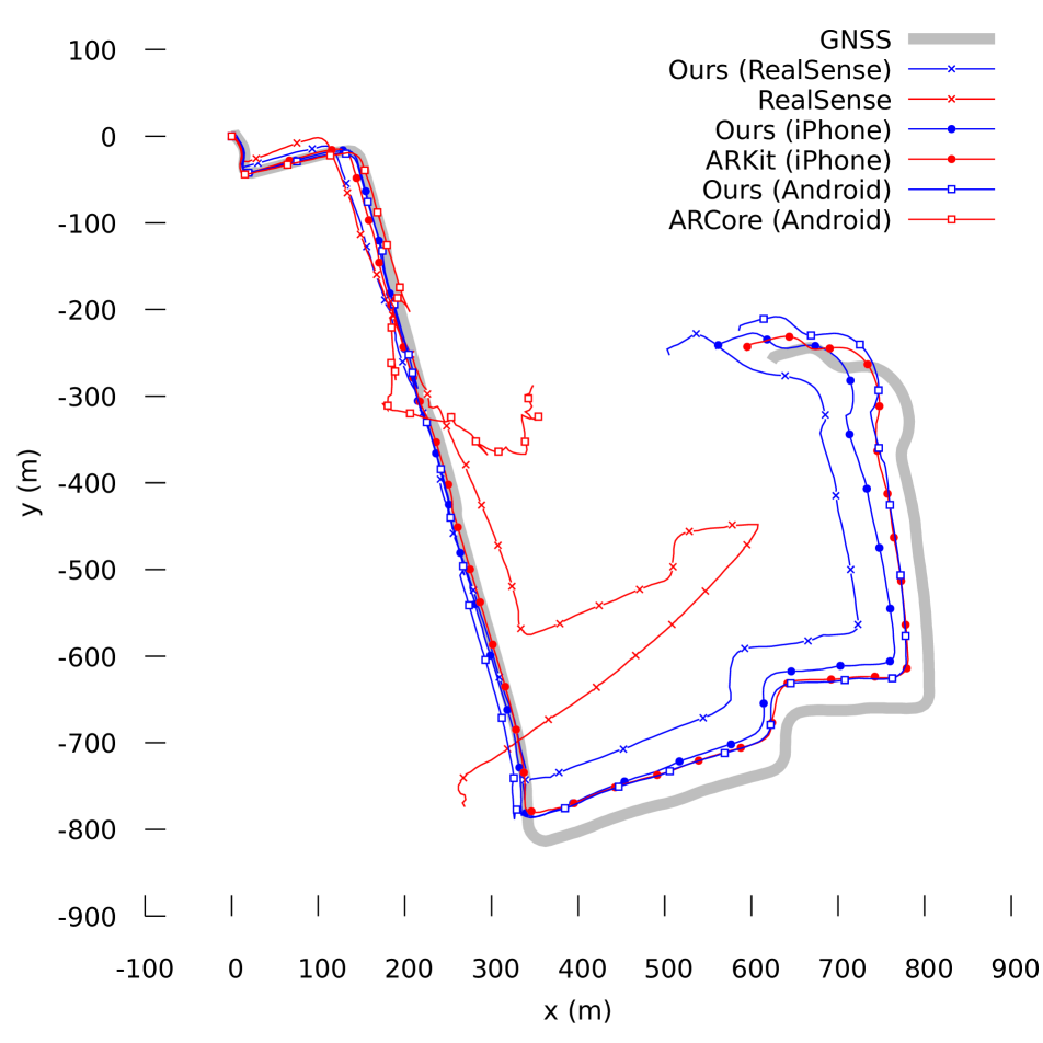
(a) Vehicular (cf. Fig. 3). Maximum velocity ${\sim}$40km/h.

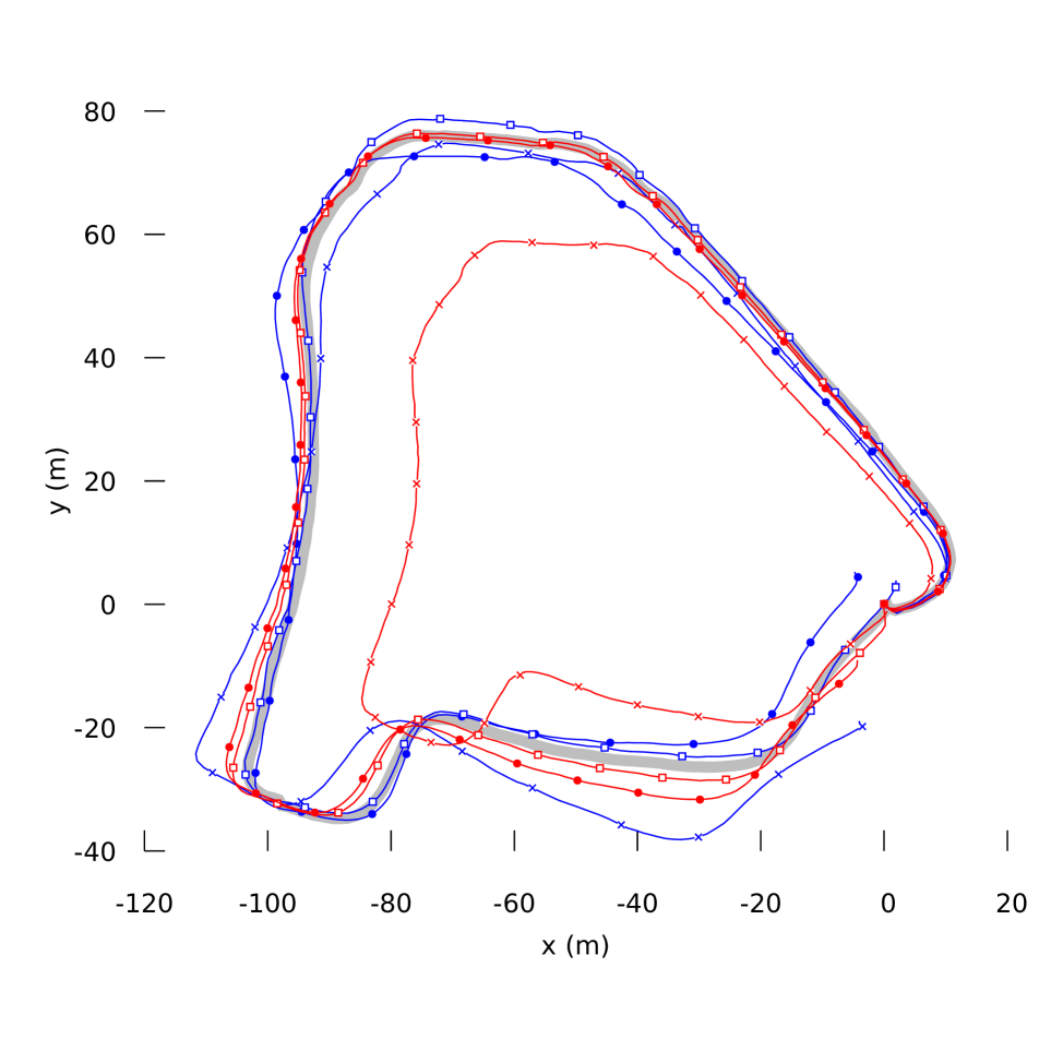
(b) Walking

Figure 4: Comparison to commercial solutions. The lines with the same symbol use the same device and input data: RealSense T265 ($\times$), iPhone 11 Pro ($\bullet$), or Huawei Mate 20 Pro ($\Box$). Blue line is our result and red is a commercial solution on the same device.

Table 5: SenseTime Benchmark, online, RMSE in millimeters.

Method	A0	A1	A2	A3	A4	A5	A6	A7	Mean
OKVIS	71.7	87.7	68.4	22.9	147	77.9	63.9	47.5	73.4
VINS-Mono	63.4	80.7	74.8	20	18.7	42.5	26.2	18.2	43.1
SenseSLAM v1.0	59	55.1	36.4	17.8	15.6	34.8	20.5	10.8	31.2
Ours	49.9	30	36	22.2	19.6	37.8	29.3	17.3	30.3

4.2 TUM VI and SenseTime VISLAM

We also evaluate our method on the room subset of the TUM VI benchmark [32] (Table 4) and the SenseTime VISLAM Benchmark [12] (Table 5) which measures the performance of monocular VISLAM with smartphone data. Both benchmarks measure post-processed SLAM performance using the RMS-ATE-$SE(3)$ metric. In TUM VI Room, we rank second, after ORB-SLAM3. In the SenseTime benchmark, we outperform the authors’ own proprietary method, SenseSLAM, on the average. More parameter configurations are presented in Sec. B.2.

4.3 Commercial comparison dataset

To evaluate the performance of our method compared to (consumer-grade) commercial solutions, we collected a custom dataset using the equipment depicted in Fig. 3. Each of the devices features a commercial VISLAM algorithm, whose outputs can be recorded, together with the camera and IMU data the device observes. This allows us to compare the accuracy of our approach to the outputs of each commercial method with the same input.

Fig. 4 shows the output trajectories of the experiment for two different sequences: Fig. 4(a) shows a vehicular test, where devices were attached to a car, exactly as shown in Fig. 3. In Fig. 4(b), the same devices were rigidly attached to a short rod and carried by a walking person.

While all methods performed relatively well in the walking sequence, this is not the case in the more challenging vehicular test, which is not officially supported by any of the tested devices. However, our method (and notably, also ARKit) are able to produce stable tracking in all cases. We also clearly outperform Intel RealSense in both sequences.

5 Discussion and conclusions

We demonstrated how the PIVO framework could be extended to stereoscopic data and improved into a high-performance independent VIO method. Furthermore, we demonstrated a novel scheme for extending it with a parallel, loosely-coupled SLAM module. The resulting hybrid method outperforms the previous state-of-the-art in real-time stereo tracking.

The measurement of VIO-only performance is also relevant since the relative value of different VISLAM capabilities are dependent on the use case. For example, in vehicular setting where GNSS-VIO fusion is utilized to perform tracking during GPS breaks, e.g., in tunnels; loop closures or local visual consistency may be irrelevant compared to uncertainty quantification and long-range accuracy. In this case, we presume that a light-weight VIO solution is more suitable than full VISLAM. We also demonstrated the feasibility of our method for vehicular tracking.

With slight trade-off for accuracy, real-time performance was demonstrated on a Raspberry Pi without the use of GPU, VPU or ISP resources, which could further improve the speed and energy consumption of visual processing. The alternative approaches report similar real-time accuracy only on high-end desktop CPUs.

Note that several aspects of our VIO are simplified compared to other recent publications. In particular, the initialization presented in Sec. 3.2 is extremely simple compared to the intricate mechanisms in [5] and [6]; we do not use the First–Estimate Jacobian methodology [11], nor model orientations as probability distributions on the $SO(3)$ manifold [10]. Implementing some of these techniques could further improve the accuracy of this approach.

Similarly to BASALT, our SLAM module lacks a separate loop closure procedure, since on the tested datasets, the low online drift could always be corrected in other SLAM steps. However, a loop closure approach similar to [19] could be valuable in challenging, large-scale benchmarks.

For an open-source implementation of the HybVIO method, see https://github.com/SpectacularAI/HybVIO.

Acknowledgments

We would like to thank Johan Jern for his contribution to the early versions of our SLAM module, and Iurii Mokrii for his contribution to our stereo code base.

Appendix

Appendix A Examples and experiment details

Differentiation example

Consider the case where the triangulation is performed using two poses $\bm{\pi}^{(1)}$, $\bm{\pi}^{(2)}$ in the stereo setup:

$$\mathbf{p}^{*} ={\rm TRI}(\bm{\pi}^{(1)},\bm{\pi}^{(2)},\mathbf{y}^{1,L},\mathbf{y}^{1,R},\mathbf{y}^{2,L},\mathbf{y}^{2,R})$$

$$={\rm TRI}_{\rm rays}(\mathbf{p}_{L,1},\mathbf{r}_{L,1},\mathbf{p}_{L,2},\mathbf{r}_{L,2},\mathbf{p}_{R,1},\mathbf{r}_{R,1},\mathbf{p}_{R,2},\mathbf{r}_{R,2}),$$

where the ray origin $\mathbf{p}_{C,j}(\bm{\pi}^{(j)})$ and bearing $\mathbf{r}_{C,j}=\mathbf{R}_{C}(\mathbf{q}^{(j)})\phi_{C}(\mathbf{y}^{j,C})$ can be computed from Eq. 9. Then the Jacobian of the triangulated point $\mathbf{p}^{*}$ with respect to $\mathbf{p}^{(1)}$ can be computed using the chain rule as

$$\frac{\partial\mathbf{p}^{*}}{\partial\mathbf{p}^{(1)}}=\frac{\partial{\rm TRI}_{\rm rays}}{\partial\mathbf{p}_{L,1}}+\frac{\partial{\rm TRI}_{\rm rays}}{\partial\mathbf{p}_{R,1}},$$ (A1)

because $\frac{\partial\mathbf{p}_{C,1}}{\partial\mathbf{p}^{(1)}}=I_{3}$ and $\frac{\partial\mathbf{a}}{\partial\mathbf{p}^{(1)}}=\mathbf{0}_{3}$ for all other arguments $\mathbf{a}$ of ${\rm TRI}_{\rm rays}$. The other blocks in the full Jacobian can be computed in a similar manner.

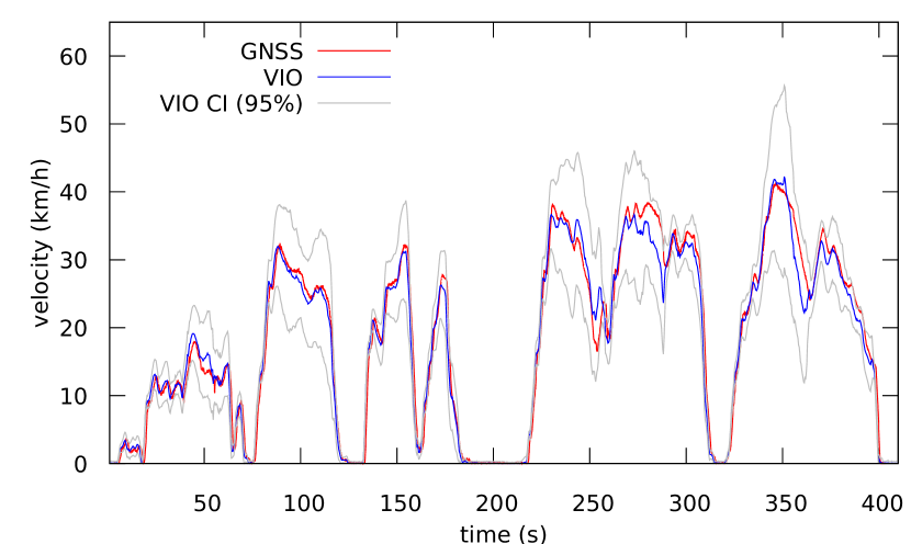
Figure A1: VIO velocity estimate for Fig. 4(a), HybVIO on ARKit

Quaternion update by angular velocity

If $\bm{\omega}=(\omega_{x},\omega_{y},\omega_{z})$ represents a constant angular velocity, then a world-to-local quaternion $\mathbf{q}=(q_{w},q_{x},q_{y},q_{z})^{\top}$ representing the orientation of a body transforms as

$$\mathbf{q}(t_{0}+\Delta t)=\bm{\Omega}[\bm{\omega}\Delta t]\mathbf{q}(t_{0})$$ (A2)

where

$$\bm{\Omega}[\mathbf{u}]:=\exp\left[-\frac{1}{2}\begin{pmatrix}0&-u_{x}&-u_{y}&-u_{z}\\ u_{x}&0&-u_{z}&u_{y}\\ u_{y}&u_{z}&0&-u_{x}\\ u_{z}&-u_{y}&u_{x}&0\end{pmatrix}\right].$$ (A3)

Note that the matrix looks different if a local-to-world quaternion representation is used (cf. [39]).

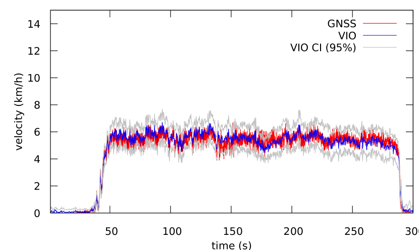
Figure A2: VIO velocity estimate for Fig. 4(b), HybVIO on ARKit

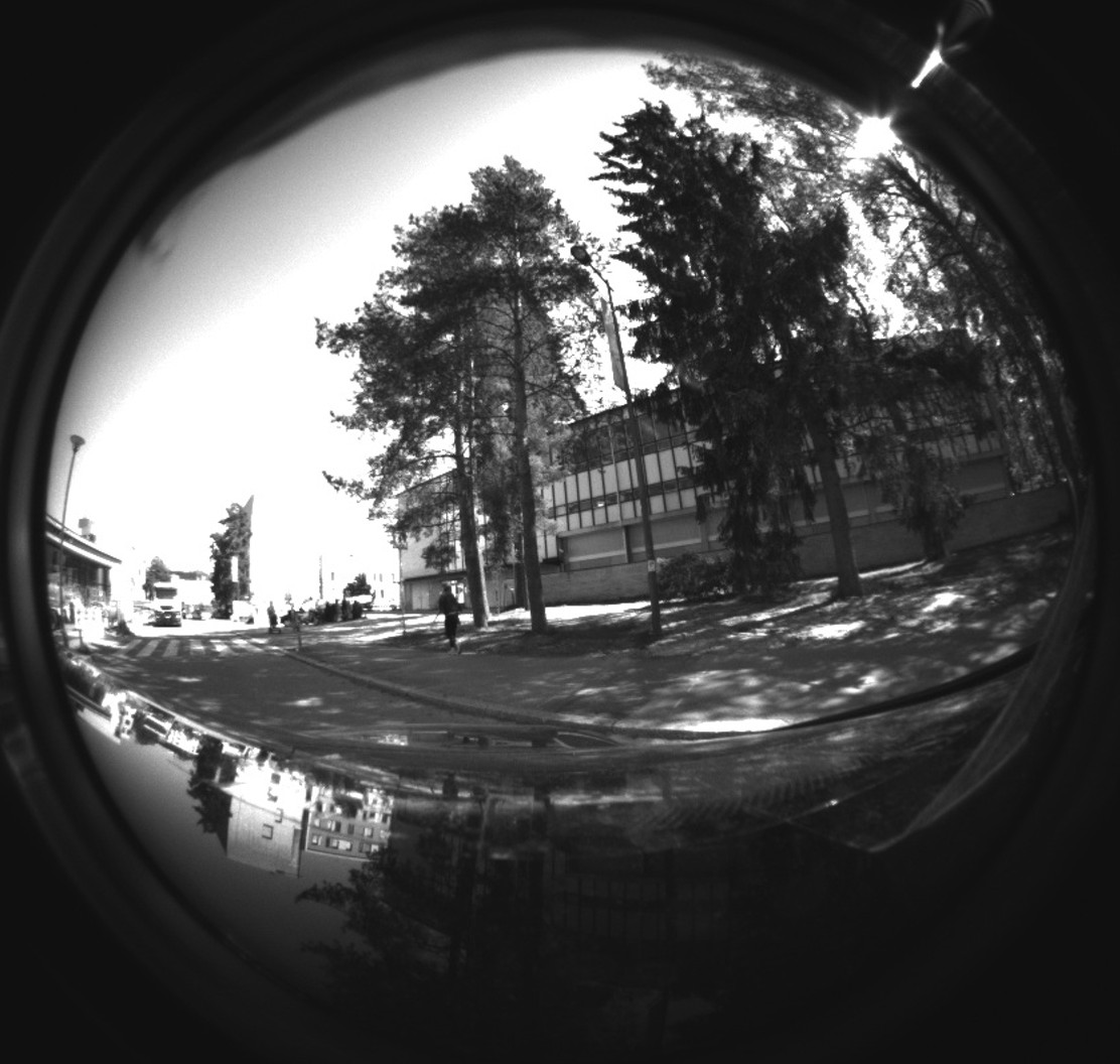
(a) Intel RealSense T265 (left camera)

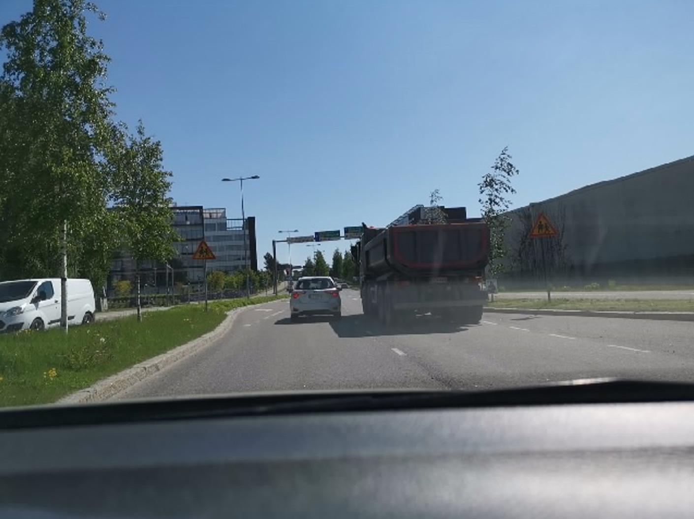
(b) Huawei Mate 20 Pro (through ARCore)

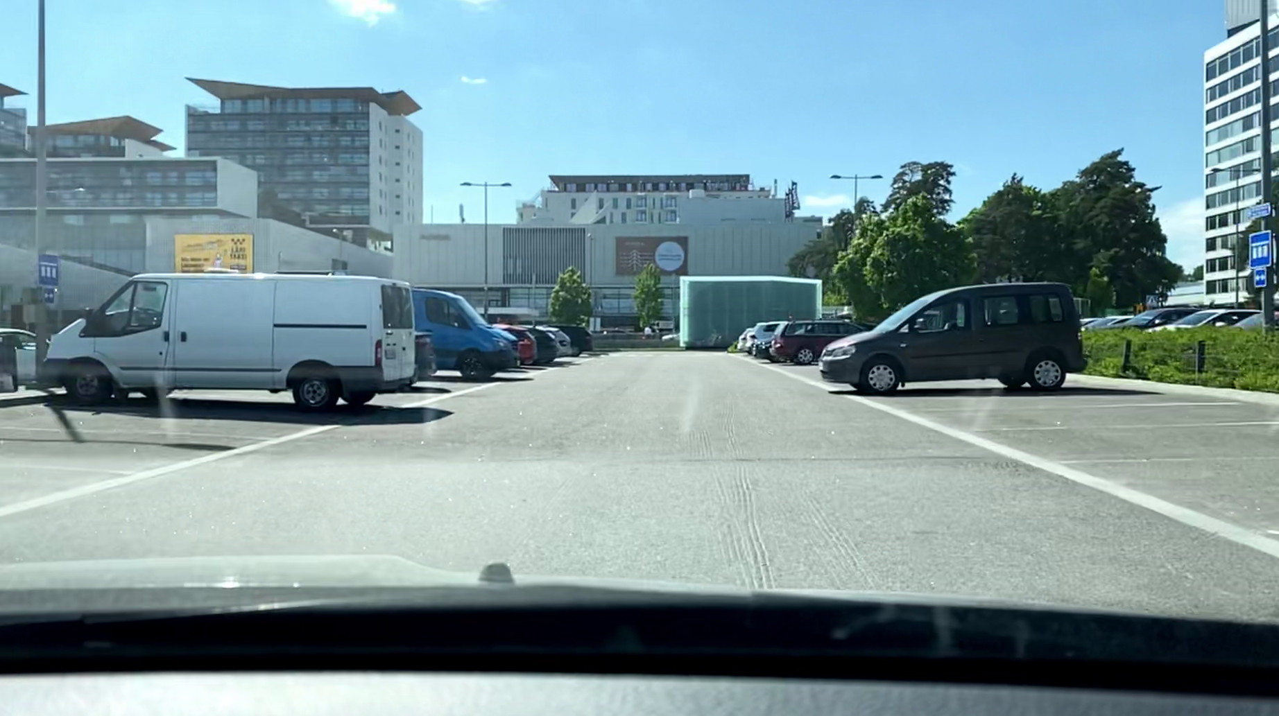
(c) iPhone 11 Pro (through ARKit)

Figure A3: Example camera views in the vehicular experiment Fig. 4(a). Reflections from the hood or windshield are visible in all images, and especially prominent in the RealSense fisheye camera.

(a) Devices, recorded as in Fig. 3

(b) Example camera view: Huawei Mate 20 Pro (through ARCore)

Figure A4: Walking experiment setup Fig. 4(b)

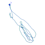
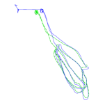
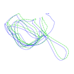
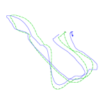
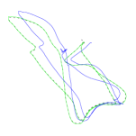
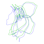
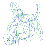
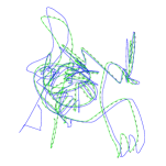
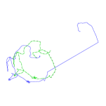
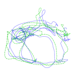
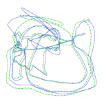
(a) ORB-SLAM3. Due to successful loop closures, the method eventually recovers and is able to produce accurate post-processed trajectories.

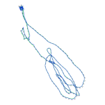
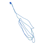
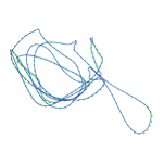
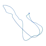
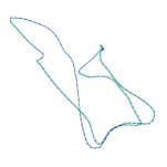
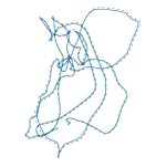
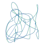
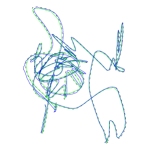
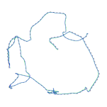
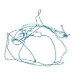
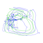
(b) BASALT

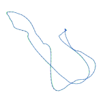
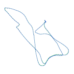
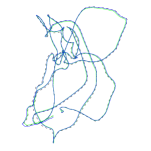
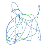
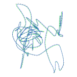
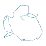
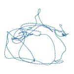
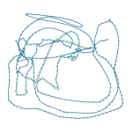
(c) HybVIO (normal SLAM / post-processed SLAM)

Figure B1: Online (blue) and post-processed (green) trajectories in EuRoC MAV stereo mode, compared to ground truth (dashed) for three different methods. Our method and BASALT produce good results in both online and post-processed modes.

Appendix B Additional experiments

B.1 Comparison to ORB-SLAM3 and BASALT

We processed the EuRoC dataset using the publicly available source code of ORB-SLAM and BASALT to compare execution times and reproduce the metrics reported in [5, 41]. The ORB-SLAM3 example code was modified to output its intermediary results, namely the latest key frame pose after each input frame, without any changes to the actual algorithm. The results are presented in Table B1.

All tests were performed on the same machine (the Ryzen setup described in Sec. 4.1) using two configurations: In the first, unrestricted configuration, the methods were allowed to utilize all 12 CPU cores in the system in parallel. BASALT was most efficiently parallelized and its processing time per frame was significantly lower than in the other methods. In the second configuration, we restricted the entire process (including input decoding) to use only 2 parallel CPU cores. In this mode, the processing times of the three methods were comparable.

The common results in Table B1 are similar to those reported in [5, 41] (and reproduced in Table 2). None of the methods (including ours) yield strictly equal results on different machines, which can explain the small remaining discrepancies. ORB-SLAM3 outputs also varied significantly between runs, but the online instability seen in Fig. B1 was consistently observed.

B.2 Ablation studies

An ablation study equivalent to Table 3 for the TUM Room dataset is presented in Table B2. In the monocular case, the results are mixed: disabling individual novel features does not consistently improve the metrics, and the simple postprocessing actually degrades the SLAM results. However, most of our configurations, notably also Fast stereo VIO, outperform all previous methods except ORB-SLAM3 (cf. Table 4)

The SenseTime benchmark results in Table B3 are more consistent and similar to Table 3: the novel features are all beneficial and the baseline PIVO implementation is not stable. However, our simple post-processing method is not able to improve the results compared to the online case.

Table B4 studies the effect of varying the parameters presented in Table 1 individually. Deviations from the selected parameters caused degraded metrics, except increasing $n_{\rm BA}$ improves the baseline results. However, this larger bundle adjustment problem is too heavy for the real-time use case and therefore we only use it in the post-processed setting.

Table B1: EuRoC computational times and RMSE in different methods (stereo SLAM). Also shown in Fig. B1.

														Ryzen frame time (ms)
	Method	MH01	MH02	MH03	MH04	MH05	V101	V102	V103	V201	V202	V203	Mean	all CPUs	2 CPUs
online	Ours(1)	0.088	0.080	0.038	0.071	0.108	0.044	0.035	0.040	0.075	0.041	0.052	0.061	32	47
	ORB-SLAM3	0.094	1.229	1.124	1.887	2.177	0.698	2.036	0.529	3.488	1.498	0.445	1.382	56	78
	BASALT	0.080	0.052	0.078	0.106	0.120	0.045	0.058	0.088	0.035	0.073	0.897	0.148	5	36
post-pr.	Ours(3)	0.048	0.028	0.037	0.056	0.066	0.038	0.035	0.037	0.031	0.029	0.044	0.041	52	95
	ORB-SLAM3	0.033	0.030	0.031	0.056	0.100	0.036	0.014	0.025	0.037	0.016	0.019	0.036	56	78
	BASALT	0.085	0.065	0.056	0.105	0.099	0.046	0.033	0.035	0.041	0.028	0.175	0.070	14	66

Table B2: Different configurations of HybVIO on the TUM Room dataset (cf. Table 3 and Table 4).

		Method	R1	R2	R3	R4	R5	R6	Mean
		Normal SLAM	0.016	0.013	0.011	0.013	0.02	0.01	0.014
online	stereo	Normal VIO	0.05	0.053	0.041	0.042	0.082	0.033	0.050
		$\smallsetminus$ Eq. 5	0.072	0.052	0.037	0.042	0.11	0.058	0.062
		Fast VIO	0.075	0.064	0.074	0.041	0.07	0.037	0.060
		$\smallsetminus$ Eq. 18	0.09	0.11	0.055	0.052	0.065	0.083	0.076
	mono	Normal SLAM	0.02	0.02	0.17	0.018	0.019	0.017	0.044
		Normal VIO	0.08	0.06	0.17	0.036	0.079	0.06	0.080
		$\smallsetminus$ RANSAC	0.065	0.072	0.092	0.058	0.06	0.049	0.066
		$\smallsetminus$ Eq. 4	0.089	0.062	0.23	0.057	0.094	0.07	0.101
		$\smallsetminus$ Eq. 6	0.09	0.066	0.21	0.05	0.069	0.049	0.089
		$\smallsetminus$ Sec. 3.9	0.087	0.06	0.14	0.046	0.079	0.06	0.078
		$\smallsetminus$ Eq. 5	0.083	0.083	0.081	0.07	0.066	0.068	0.075
		PIVO baseline	0.075	0.077	0.11	0.051	0.14	0.071	0.088
		Fast VIO	0.086	0.061	0.066	0.077	0.061	0.07	0.070
		$\smallsetminus$ Eq. 18	0.09	0.062	0.12	0.082	0.08	0.051	0.082
post-pr.		Stereo SLAM	0.042	0.041	0.028	0.025	0.061	0.02	0.036
		Mono SLAM	0.039	0.033	0.16	0.032	0.039	0.026	0.055

Table B3: Different configurations of HybVIO in the SenseTime benchmark (cf. Table 3 and Table 5).

	Method	A0	A1	A2	A3	A4	A5	A6	A7	Mean
	Normal SLAM	49.9	30	36	22.2	19.6	37.8	29.3	17.3	30.3
online	Normal VIO	63.5	53.1	53.9	28.1	26.3	75.6	29.7	26.6	44.6
	$\smallsetminus$ RANSAC	73.1	109	59	27.6	24.2	65.8	30	22	51.3
	$\smallsetminus$ Eq. 4	171	272	208	40.8	83.6	170	116	120	148
	$\smallsetminus$ Eq. 6	69.5	70.9	47.8	33.9	31.4	74.9	32.2	43.1	50.5
	$\smallsetminus$ Sec. 3.9	87.7	764	149	75.6	158	351	310	328	278
	$\smallsetminus$ Eq. 5	75.2	46.3	53	27.7	34	72.9	31.2	27.6	46
	PIVO baseline	166	1150	225	219	242	472	109	239	353
	Fast VIO	47.2	59.6	43.1	25.8	46	60.5	30.6	40	44.1
	$\smallsetminus$ Eq. 18	80	73.4	89.1	26.8	50	119	38	50.2	65.8
Post-pr. SLAM		63.9	28.4	28.5	23.2	42.7	23.3	22.2	18.1	31.3

Table B4: Effect of individual parameters in Table 1 on the mean RMSE and frame time in EuRoC. The baseline is Normal SLAM.

Altered parameter	Value	RMSE	Frame time (ms)
baseline(1)		0.061	35
feature detector	FAST	0.067	33
subpix. adjustment	off	0.065	33
max. features	70	0.066	19
max. features	100	0.065	23
max. features	300	0.061	48
max. itr.	8	0.064	35
max. itr.	40	0.066	36
window size	13	0.062	34
window size	51	0.07	37
$n_{\rm a}$	30	0.062	43
$n_{\rm{target}}$	5	0.063	33
$n_{\rm{target}}$	10	0.064	37
$n_{\rm{target}}$	30	0.061	34
$n_{\rm{FIFO}}$	20	0.068	36
$n_{\rm{FIFO}}$	14	0.31	35
$n_{\rm{BA}}$	50	0.053	42
$n_{\rm{BA}}$	100	0.055	79
$n_{\rm{matching}}$	35	0.06	36
$n_{\rm{matching}}$	50	0.06	36

B.3 Vehicular

This section includes additional vehicular experiments (Fig. B2 and Fig. B3) using the setup shown in Fig. 3, as well as results from a slightly modified setup (shown in Fig. 5(a)), where we have added ZED 2 as a new device.

ZED 2 also has a proprietary VISLAM capability, but it did not perform well in the vehicular test cases (see Fig. B4 for an example) and we omitted it in the other sequences to avoid frame drop issues experienced when recording ZED 2 input and tracking output data simultaneously. The ZED 2 camera data was recorded at 60FPS but utilized at 30FPS.

We used the normal VIO mode (see Table 1) for all vehicular experiments. Stereo mode was used with both stereo camera devices.

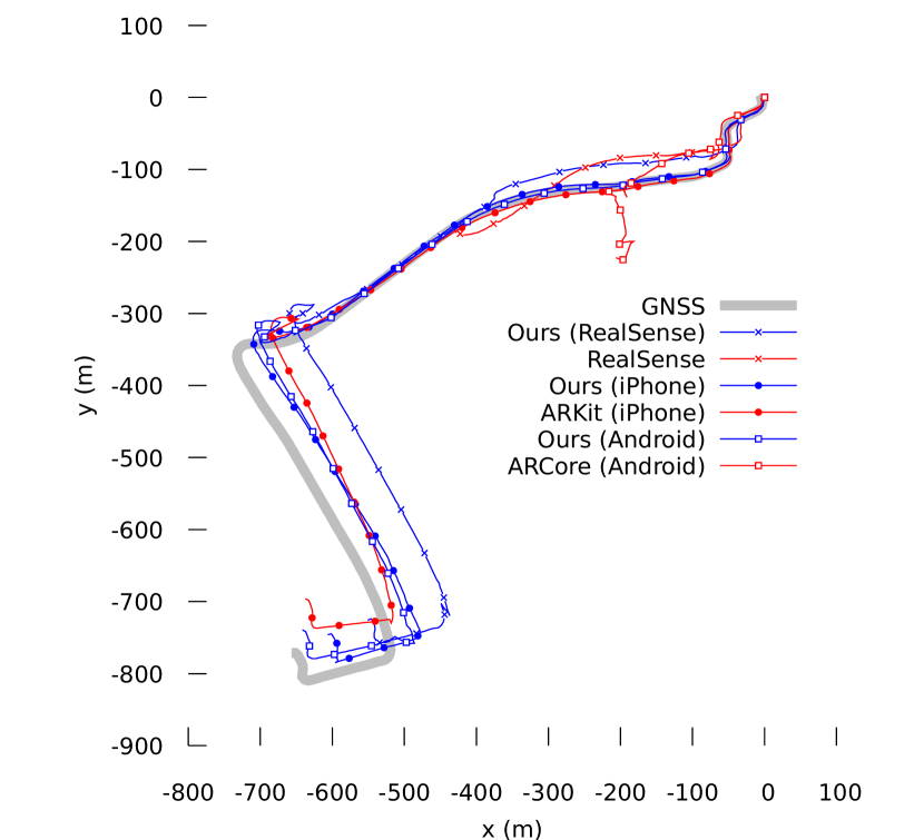
(a) Position

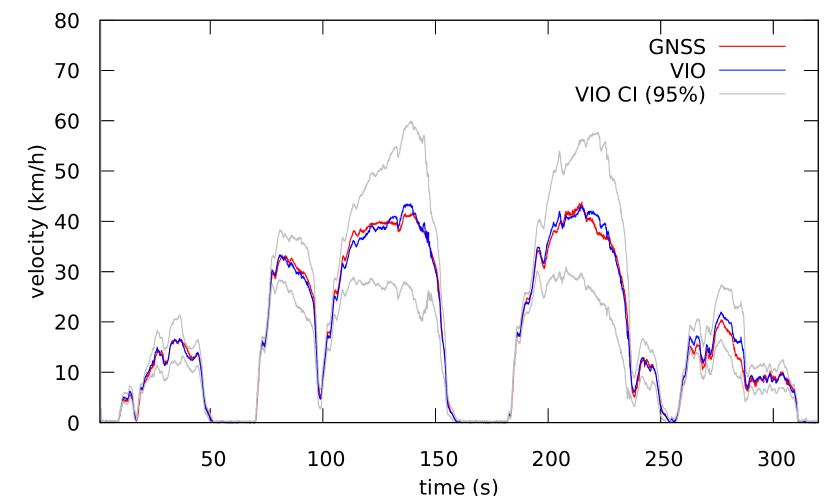
(b) VIO velocity estimate, HybVIO on ARKit

Figure B2: Vehicular experiment 2, using the setup in Fig. 3

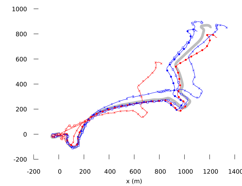
(a) Position

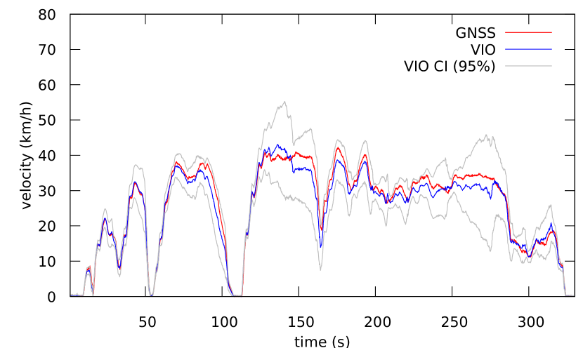
(b) VIO velocity estimate, HybVIO on ARKit

Figure B3: Vehicular experiment 3, using the setup in Fig. 3

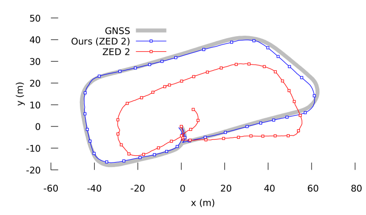
Figure B4: Vehicular experiment 4. A slow drive around a parking lot, recording the setup shown in Fig. 5(a). Unlike the following experiments with ZED 2, the proprietary tracking output from ZED 2 is compared to HybVIO using the same input data.

(a) Second car experiment setup: GNSS is used as ground truth. The iPhone records ARKit and its input data simultaneously. ZED 2 records camera (stereo rolling shutter at 60FPS) and IMU data.

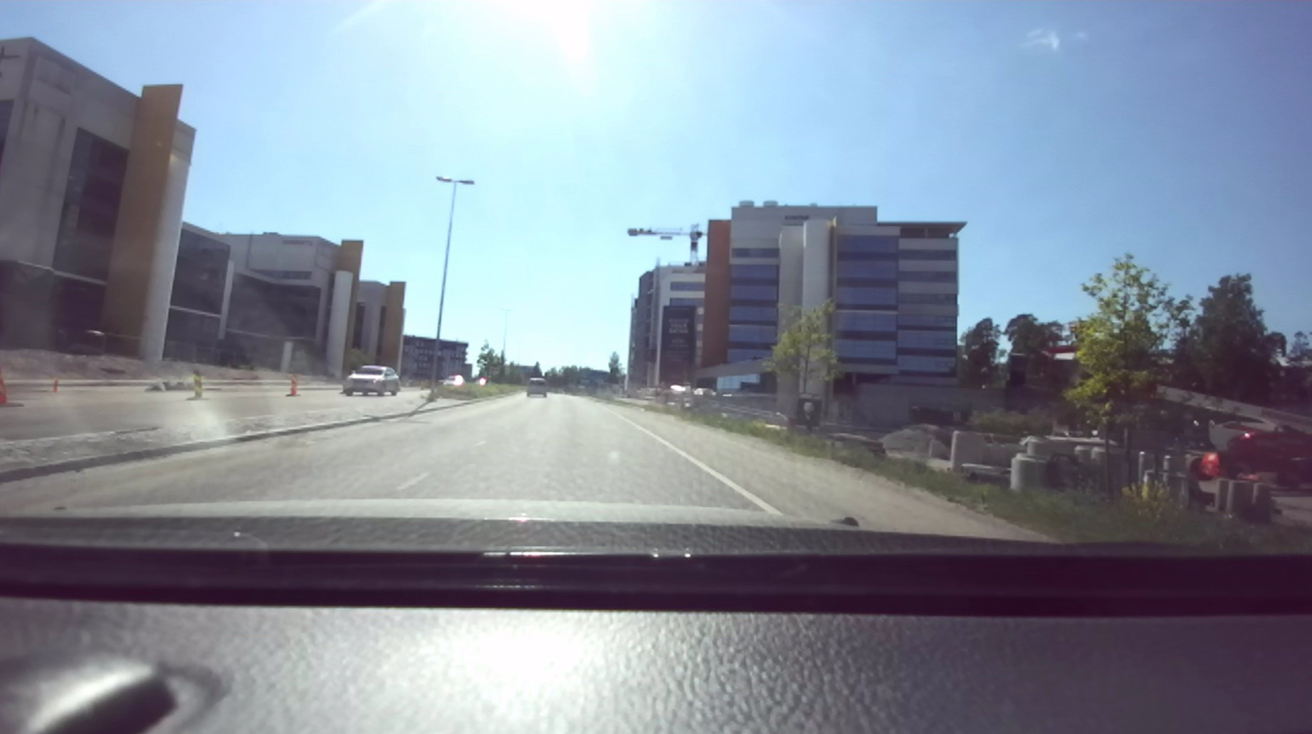
(b) Example ZED 2 left camera view corresponding to (TODO: Use cref instead of ref.)

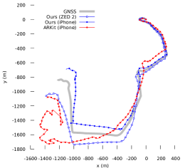
(c) Vehicular experiment 5

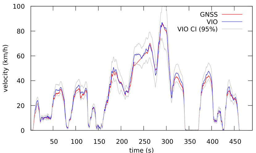
(d) VIO velocity estimate for (TODO: Use cref instead of ref.), HybVIO on ZED 2. A GNSS outage is visible as a straight line segment near the 250 seconds mark.

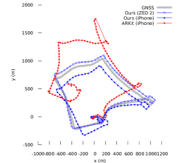
(e) Vehicular experiment 6

(f) VIO velocity estimate for (TODO: Use cref instead of ref.), HybVIO on ZED 2. A GNSS outage is visible after 700 seconds.

Figure B5: Additional vehicular experiments with higher velocities ($\sim$ 80km/h), in which ARKit also fails. In this case, HybVIO performs better on the same data.

Appendix C Supplementary videos

1. euroc-mh-05-difficult_fast-VIO
   (https://youtu.be/ou1DrtjPx1Q) A screen recording from a laptop running HybVIO in fast VIO mode (cf. Table 1) on the EuRoC MAV sequence MH-05. The final trajectory also appears in Fig. 1.

   The visual tracking and update status are visualized on the left and right camera frames, similarly to Fig. 2 but with different colors: reprojections are in white, successfully updated tracks in black and failed tracks in blue. The lower part of the video shows the online track (x and y coordinates) in blue and ground truth in orange. Triangulated points are shown as small black circles. The online track is automatically rotated to optimally match the ground truth, after approximately 10 seconds.

2. euroc-v1-02-medium_normal-SLAM
   (https://youtu.be/7j1rYoD_pPc) Similar to the previous video, but HybVIO is running in the normal SLAM mode on the sequence V1-02. The triangulated SLAM map points in the current local map are shown as yellow in the lower right subimage, and their reprojections as orange on the (left) camera image. The LK-tracked features (cf. Alg. 1) that correspond to SLAM map points are shown as yellow circles on the camera image.

   The left part of the video shows the SLAM map. Key frame camera poses are shown in light blue. In the beginning, the triangulated points in the local map are shown in red. At time 00:27, the colors are changed to show the observation direction of the map point. The covisibility graph is shown first at 00:15, in a yellow-green color. We consider a pair of key frames adjacent in this graph if they observe at least $N_{\rm neigh}=10$ common map points.

3. vehicular-experiment-6
   (https://youtu.be/iVNicL_S14Y) Visualizes the vehicular experiment in Fig. 5(e) on a map (HybVIO on ZED 2). The VIO trajectory is aligned using a fixed angle and offset. The local VIO trajectory is formed using the pose trails (cf. Sec. 3.1) in the VIO state. The traffic light stops are automatically cut from the video (based on the VIO velocity estimate). Despite generally good RTK-GNSS coverage in the area, the sequence includes a GNSS outage in a tunnel, starting at time 02:32 in the video.

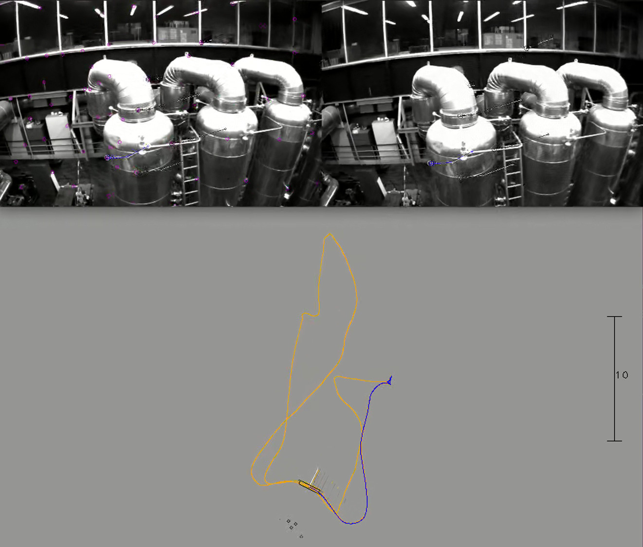
(a) euroc-mh-05-difficult_fast-VIO

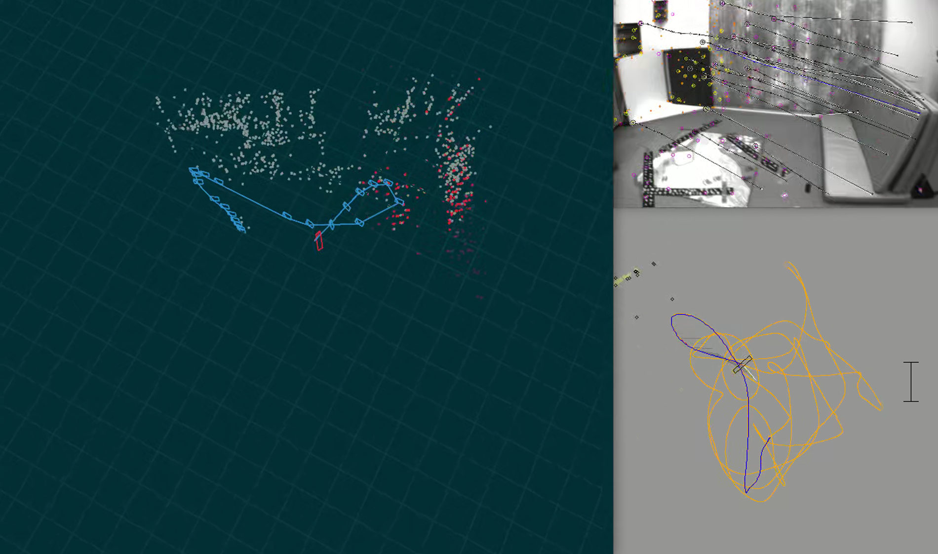
(b) euroc-v1-02-medium_normal-SLAM

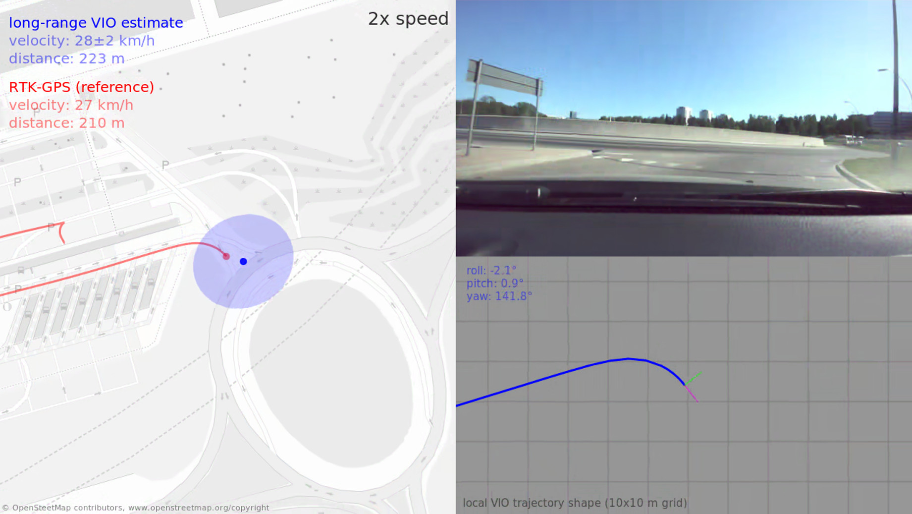
(c) vehicular-experiment-6

Figure C1: Screenshots from the supplementary videos

References

- [1] Jinqiang Bai, Junqiang Gao, Yimin Lin, Zhaoxiang Liu, Shiguo Lian, and Dijun Liu. A novel feedback mechanism-based stereo visual-inertial SLAM. IEEE Access, 7:147721–147731, 2019.
- [2] Michael Bloesch, Sammy Omari, Marco Hutter, and Roland Yves Siegwart. Robust visual inertial odometry using a direct EKF-based approach. In Proceedings of the International Conference on Intelligent Robots and Systems (IROS), pages 298–304, Hamburg, Germany, 2015.
- [3] Gary Bradski. The OpenCV library. Dr. Dobb’s Journal of Software Tools, 2000.
- [4] Michael Burri, Janosch Nikolic, Pascal Gohl, Thomas Schneider, Joern Rehder, Sammy Omari, Markus W Achtelik, and Roland Siegwart. The EuRoC micro aerial vehicle datasets. International Journal of Robotics Research, 35:1157–1163, 2016.
- [5] Carlos Campos, Richard Elvira, Juan J. Gómez, José M. M. Montiel, and Juan D. Tardós. ORB-SLAM3: An accurate open-source library for visual, visual-inertial and multi-map SLAM. IEEE Transactions on Robotics, 2021.
- [6] Carlos Campos, José M.M. Montiel, and Juan D. Tardós. Inertial-only optimization for visual-inertial initialization. In 2020 IEEE International Conference on Robotics and Automation (ICRA), pages 51–57, 2020.
- [7] Ronald Clark, Sen Wang, Hongkai Wen, Andrew Markham, and Niki Trigoni. VINet: Visual-inertial odometry as a sequence-to-sequence learning problem. Proceedings of the AAAI Conference on Artificial Intelligence, 31(1), Feb. 2017.
- [8] Andrew J. Davison, Ian D. Reid, Nicholas D. Molton, and Olivier Stasse. MonoSLAM: Real-time single camera SLAM. IEEE Transactions on Pattern Analysis and Machine Intelligence, 29(6):1052–1067, 2007.
- [9] Jakob Engel, Thomas Schöps, and Daniel Cremers. LSD-SLAM: Large-scale direct monocular SLAM. In Proceedings of European Conference on Computer Vision (ECCV), pages 834–849, Zurich, Switzerland, 2014.
- [10] Christian Forster, Luca Carlone, Frank Dellaert, and Davide Scaramuzza. On-manifold preintegration for real-time visual–inertial odometry. Transactions on Robotics, 33(1):1–21, 2017.
- [11] Guoquan P. Huang, Anastasios I. Mourikis, and Stergios I. Roumeliotis. A First-Estimates Jacobian EKF for improving SLAM consistency. In Oussama Khatib, Vijay Kumar, and George J. Pappas, editors, Experimental Robotics, pages 373–382, Berlin, Heidelberg, 2009. Springer Berlin Heidelberg.
- [12] Li. Jinyu, Bangbang Yang, Danpeng Chen, Nan Wang, Guofeng Zhang, and Hujun Bao. Survey and evaluation of monocular visual-inertial SLAM algorithms for augmented reality. Journal of Virtual Reality & Intelligent Hardware, 1(4):386–410, 2019.
- [13] Kenichi Kanatani. Analysis of 3-D rotation fitting. IEEE Transactions on Pattern Analysis and Machine Intelligence, 16(5):543–549, 1994.
- [14] Juho Kannala and Sami S. Brandt. A generic camera model and calibration method for conventional, wide-angle, and fish-eye lenses. IEEE Trans. Pattern Anal. Mach. Intell., 28(8):1335–1340, 2006.
- [15] Stefan Leutenegger, Simon Lynen, Michael Bosse, Roland Siegwart, and Paul Furgale. Keyframe-based visual–inertial odometry using nonlinear optimization. International Journal of Robotics Research, 34(3):314–334, 2015.
- [16] Mingyang Li and Anastasios I Mourikis. Optimization-based estimator design for vision-aided inertial navigation. In Robotics: Science and Systems (RSS), pages 241–248. Berlin Germany, 2013.
- [17] Bruce D. Lucas and Takeo Kanade. An iterative image registration technique with an application to stereo vision. In Proceedings of the International Conference on Artificial Intelligence (IJCAI), pages 674–679. Vancouver, BC, Canada, 1981.
- [18] Anastasios I. Mourikis and Stergios I. Roumeliotis. A multi-state constraint Kalman filter for vision-aided inertial navigation. In Proceedings of the International Conference on Robotics and Automation (ICRA), pages 3565–3572, Rome, Italy, 2007.
- [19] Raul Mur-Artal, J. Montiel, and Juan Tardos. ORB-SLAM: a versatile and accurate monocular slam system. IEEE Transactions on Robotics, 31:1147–1163, 10 2015.
- [20] Raul Mur-Artal and Juan D. Tardos. ORB-SLAM2: An open-source SLAM system for monocular, stereo, and RGB-D cameras. IEEE Transactions on Robotics, 33(5):1255–1262, Oct 2017.
- [21] David Nistér. An efficient solution to the five-point relative pose problem. IEEE Trans. Pattern Anal. Mach. Intell., 26(6):756–777, 2004.
- [22] David Nistér, Oleg Naroditsky, and James Bergen. Visual odometry. In Proceedings of the Computer Society Conference on Computer Vision and Pattern Recognition (CVPR), volume 1, pages I–652, Washington, DC, US, 2004.
- [23] Mrinal K. Paul, Kejian Wu, Joel A. Hesch, Esha D. Nerurkar, and Stergios I. Roumeliotis. A comparative analysis of tightly-coupled monocular, binocular, and stereo VINS. In IEEE International Conference on Robotics and Automation, ICRA, 2017.
- [24] Tong Qin, Peiliang Li, and Shaojie Shen. VINS-Mono: A robust and versatile monocular visual-inertial state estimator. IEEE Transactions on Robotics, 34(4):1004–1020, 2018.
- [25] Tong Qin and Shaojie Shen. Online temporal calibration for monocular visual-inertial systems. In Proceedings of the International Conference on Intelligent Robots and Systems (IROS), pages 3662–3669. IEEE, 2018.
- [26] Xiaochen Qiu, Hai Zhang, and Wenxing Fu. Lightweight hybrid visual-inertial odometry with closed-form zero velocity update. Chinese Journal of Aeronautics, 2020.
- [27] Meixiang Quan, Songhao Piao, Minglang Tan, and Shi-Sheng Huang. Accurate monocular visual-inertial SLAM using a map-assisted EKF approach. IEEE Access, 7:34289–34300, 2019.
- [28] Antoni Rosinol, Marcus Abate, Yun Chang, and Luca Carlone. Kimera: An open-source library for real-time metric-semantic localization and mapping. In International Conference on Robotics and Automation (ICRA), 2020.
- [29] Edward Rosten and Tom Drummond. Machine learning for high-speed corner detection. In Proceedings of European Conference on Computer Vision (ECCV), pages 430–443, 2006.
- [30] Stergios I Roumeliotis and Joel W Burdick. Stochastic cloning: A generalized framework for processing relative state measurements. In Proceedings to the International Conference on Robotics and Automation (ICRA), volume 2, pages 1788–1795, 2002.
- [31] Ethan Rublee, Vincent Rabaud, Kurt Konolige, and Gary Bradski. ORB: An efficient alternative to SIFT or SURF. In Proceedings of the IEEE International Conference on Computer Vision (ICCV), pages 2564–2571, 11 2011.
- [32] David Schubert, Thore Goll, Nikolaus Demmel, Vladyslav Usenko, Jörg Stückler, and Daniel Cremers. The TUM VI benchmark for evaluating visual-inertial odometry. In Proceedings of the International Conference on Intelligent Robots and Systems (IROS), pages 1680–1687, 2018.
- [33] Jianbo Shi and Carlo Tomasi. Good features to track. In Proceedings of the IEEE Computer Society Conference on Computer Vision and Pattern Recognition (CVPR), pages 593–600, 1994.
- [34] Arno Solin, Santiago Cortes, Esa Rahtu, and Juho Kannala. PIVO: Probabilistic inertial-visual odometry for occlusion-robust navigation. In Proceedings of the Winter Conference on Applications of Computer Vision (WACV), pages 616–625, Los Alamitos, CA, USA, mar 2018. IEEE Computer Society.
- [35] Arno Solin, Santiago Cortes Reina, Esa Rahtu, and Juho Kannala. Inertial odometry on handheld smartphones. In Proceedings of the 21st International Conference on Information Fusion (FUSION), pages 1361–1368, 2018.
- [36] Shinya Sumikura, Mikiya Shibuya, and Ken Sakurada. OpenVSLAM: A versatile visual SLAM framework. CoRR, abs/1910.01122, 2019.
- [37] Ke Sun, Kartik Mohta, Bernd Pfrommer, Michael Watterson, Sikang Liu, Yash Mulgaonkar, Camillo J. Taylor, and Vijay Kumar. Robust stereo visual inertial odometry for fast autonomous flight. IEEE Robotics and Automation Letters, 3(2):965–972, 2018.
- [38] Petri Tanskanen, Tobias Naegeli, Marc Pollefeys, and Otmar Hilliges. Semi-direct EKF-based monocular visual-inertial odometry. In Proceedings of the International Conference on Intelligent Robots and Systems (IROS), pages 6073–6078, Hamburg, Germany, 2015.
- [39] David H. Titterton and John L. Weston. Strapdown Inertial Navigation Technology. The Institution of Electrical Engineers, 2004.
- [40] George E Uhlenbeck and Leonard S Ornstein. On the theory of the Brownian motion. Physical Review, 36(5):823, 1930.
- [41] Vladyslav Usenko, Nikolaus Demmel, David Schubert, Jörg Stückler, and Daniel Cremers. Visual-inertial mapping with non-linear factor recovery. IEEE Robotics and Automation Letters (RA-L) & Int. Conference on Intelligent Robotics and Automation (ICRA), 5(2):422–429, 2020.
- [42] Lukas von Stumberg, Vladyslav Usenko, and Daniel Cremers. Direct sparse visual-inertial odometry using dynamic marginalization. In International Conference on Robotics and Automation (ICRA), pages 2510–2517, 2018.