Off-Policy Reinforcement Learning with
Delayed Rewards

Abstract

We study deep reinforcement learning (RL) algorithms with delayed rewards. In many real-world tasks, instant rewards are often not readily accessible or even defined immediately after the agent performs actions. In this work, we first formally define the environment with delayed rewards and discuss the challenges raised due to the non-Markovian nature of such environments. Then, we introduce a general off-policy RL framework with a new $\mathcal{Q}$-function formulation that can handle the delayed rewards with theoretical convergence guarantees. For practical tasks with high dimensional state spaces, we further introduce the HC-decomposition rule of the $\mathcal{Q}$-function in our framework which naturally leads to an approximation scheme that helps boost the training efficiency and stability. We finally conduct extensive experiments to demonstrate the superior performance of our algorithms over the existing work and their variants.

1 Introduction

Deep reinforcement learning (RL) aims at maximizing the cumulative reward of a MDP. To apply RL algorithms, the reward has to be given at every state-action pair in general (i.e., $r(s,a)$). With a good and high quality reward function, RL can achieve remarkable performance, e.g. AlphaGo Zero for Go [1], DQN[2] for Atari, SAC [3] for robot control e.t.c. Recently, RL has been applied in many other real world settings beyond games and locomotion control. This includes industrial process control [4], traffic optimization [5, 6], molecular design [7] and resource allocation [8]. However, in many of these real-world scenarios, Markovian and instant per-step rewards are hard or impossible to obtain or even clearly defined. In practice, it becomes more reasonable to use a delayed reward of several consecutive steps as feedback. For example, in traffic congestion reduction [5], the amount of decreased congestion for a single traffic light switch is hard to define in practice while it is more adequate to use the average routing time consumed for the vehicles as the feedback. The latter is a delayed reward which can only be obtained after the vehicles have passed the congestion (long after a single switch). In molecular design, only the molecule formed after the final operation can provide a meaningful evaluation for the whole process [7]. In locomotion control where the feedback is generated by the interaction with the large environment, it is usually the case that the frequency of the rewards generated from the environment’s sensors is much lower than the frequency of the robot control, thus the rewards are given only every so often.

Despite the importance and prevalence of the delayed reward setting, very few previous research in RL has been focusing on problems with non-Markovian properties and delayed rewards. Besides, current RL algorithms lack theoretical guarantee under non-Markovian rewards and perform unsatisfactorily in practice [9]. Thus, in this paper, our goal is to better understand the properties of RL with delayed rewards and introduce a new algorithm that can handle the delayed reward both theoretically and practically. A key to our approach lies in the definition of the past-invariant delayed reward MDPs. Based on this definition, theoretical properties and algorithmic implications are discussed to motivate the design of a new practical algorithm, which explicitly decompose the value function into components of both historical (H) and current (C) step information. We also propose a number of ways to approximate such HC decomposition, which can be readily incorporated into existing off-policy learning algorithms. Experiments demonstrate that such approximation can improve training efficiency and robustness when rewards are delayed.

2 Problem Formulation

In order to characterize the delayed and non-Markov reward signals, we introduce the Delayed Reward Markov Decision Process (DRMDP). In this work, we focus on DRMDP that satisfies the Past-Invariant (PI) condition, which is satisfied in many real-world settings with delayed reward and will be explicitly defined in the following subsection.

2.1 Past-Invariant Delayed Reward MDPs

In DRMDP, the transition of the environment is still Markovian and the agent can observe and interact with the environment instantly. However, rewards may be non-Markovian and are delayed and observed only once every few steps. More specifically, the time steps are divided into consecutive signal intervals of random lengths, and the reward signal generated during a signal interval may depend on the a period of state-action sequence and is observed only at the end of the interval. We formally define DRMDP as follows.

Definition 1 (DRMDP).

A Delayed Reward Markov Decision Process $M=(S,A,p,q_{n},r,\gamma)$ is described by the following parameters.

1. The state and action spaces are $S$ and $A$ respectively.

2. The Markov transition function is $p(s^{\prime}|s,a)$ for each $(s,a)\in S\times A$; the initial state distribution is $p(s_{0})$.

3. The signal interval length is distributed according to $q_{n}(\cdot)$, i.e., for the $i$-th signal interval, its length $n_{i}$ is independently drawn from $q_{n}(\cdot)$.

4. The reward function $r$ defines the expected reward generated for each signal interval; suppose $\tau_{i}=\tau_{t:t+n_{i}}=(s,a)_{t:t+n_{i}}=((s_{t},a_{t}),\dots(s_{t+n-1},a_{t+n_{i}-1}))$ is the state-action sequence during the $i$-th signal interval of length $n_{i}$, then the expected reward for this interval is $r(\tau_{i})$.

5. The reward discount factor is $\gamma$.

In this work, we focus on the infinite-horizon DRMDP. We use $(\tau,n)=(\tau_{i},n_{i})_{i\in\{1,2,3,\dots\}}$ to denote a trajectory, where $\tau_{i}$ is the state-action sequence during the $i$-th signal interval and $n_{i}$ is the corresponding length. We also let $t_{i}$ be first time step of the $i$-th signal interval, i.e., $t_{i}=\sum_{j=1}^{i-1}n_{j}$. Note that the reward $r(\tau_{i})$ is revealed at time $t_{i}+n_{i}-1=t_{i+1}-1$. We finally define the discounted cumulative reward of the trajectory $(\tau,n)$ by $R(\tau,n):=\sum_{i=1}^{\infty}\gamma^{t_{i+1}-1}r(\tau_{i})$. The objective for DRMDP is to learn a policy $\pi$ that maximized the expected discounted cumulative reward $\mathcal{J}(\pi):=\mathbb{E}_{(\tau,n)\sim\pi}[R(\tau,n)]$.

Because of the non-Markovian nature of DRMDP, the Markov policy class $\{\pi=\pi(a_{t}|s_{t})\}$ might not achieve satisfactory expected discounted reward. In this work, we consider two more general policy classes $\Pi_{s}=\{\pi=\pi(a_{t}|s_{t},t-t_{i})\}$ and $\Pi_{\tau}=\{\pi=\pi(a_{t}|\tau_{t_{i}:t}\circ s_{t})\}$, where in both classes, $i=i(t)$ is the index of the signal interval that $t$ belongs to. Note that the first policy class $\Pi_{s}$ resembles the traditional type of policy $\pi(a_{t}|s_{t})$, but is augmented with an extra parameter indicting the relative index of the current time step in the signal interval. The second policy class $\Pi_{\tau}$ takes all previous steps in the current signal interval into consideration to decide the action. Regarding the power of the two policy classes, we first observe the following fact.

Fact 1.

For any DRMDP, there exists an optimal policy $\pi^{*}\in\Pi_{\tau}$. However, there exists some DRMDP such that all of its optimal policies $\pi^{*}\notin\Pi_{s}$.

Fact 1 indicates that general DRMDPs are relatively hard to solve as the agents have to search in quite a large policy space. In this work, we focus on the DRMDP with the Past-Invariant property described as follows.

Definition 2 (PI-DRMDP).

A Past-Invariant Delayed Reward Markov Decision Process is a DRMDP  $M=(S,A,p,q_{n},r,\gamma)$ whose reward function $r$ satisfies the following Past-Invariant (PI) condition: for any two trajectory segments $\tau_{1}$ and $\tau_{2}$ of the same length, and for any two equal-length trajectory segments $\tau_{1}^{\prime}$ and $\tau_{2}^{\prime}$ such that the concatenated trajectories $\tau_{a}\circ\tau_{b}^{\prime}$ are feasible under the transition dynamics $p$ for all $a,b\in\{1,2\}$, it holds that

$$r(\tau_{1}\circ\tau_{1}^{\prime})>r(\tau_{1}\circ\tau_{2}^{\prime})\iff r(\tau_{2}\circ\tau_{1}^{\prime})>r(\tau_{2}\circ\tau_{2}^{\prime}).$$

Roughly speaking, in PI-DRMDP, the relative credit for different actions at each $s_{t}$ only depends on the experience in the future and is invariant of the past. This property may relieve the agent from considering the past experience for decision making. Unfortunately, in theory, there exists some bizarre reward design that still requires the agent to take history into consideration in terms of the optimal policy. We simplify this problem in our work by only searching for policy in $\Pi_{s}$. In Appendix A, we will discuss this issue in detail. From now on, we will only discuss the polices in $\Pi_{s}$ without further specification.

A simple example of $r$ with PI condition is $r(\tau_{t:t+n})=\sum_{i=t}^{t+n-1}\hat{r}(s_{i},a_{i})$, where $\hat{r}$ is a per-step reward function. This kind of tasks is studied in many previous work [10, 11, 12]. We refer this kind of reward functions as the sum-form.

General Reward Function. In Definition 1, we define the reward as a function of the state-action sequence of its signal interval. In general, we may allow reward functions with longer input which overlap with the previous signal intervals, e.g., maximal overlapping of $c$ steps

$$r(\tau_{t_{i}-c:t_{i}+n_{i}}).$$

The theoretical analysis in Section 3.1 and the empirical method in Section 3.2 can be directly extended to this general reward function. We provide detailed discussions in Appendix A for the general definition while we only consider $c=0$ in the main text for the simplicity of the exposition.

2.2 Off-Policy RL in PI-DRMDP

Deep Reinforcement Learning has achieved great success in solving high-dimensional MDPs problems, among which the off-policy actor-critic algorithms SAC [13] and TD3 [14] are the most widely used ones. However, since the rewards are delayed and non-Markovian in PI-DRMDP, directly applying these SOTA off-policy RL algorithms faces many challenges that degrade the learning performance. In this subsection, we briefly discuss the problems that arise in critic learning based on TD3 and similar problems also exist for SAC.

First, in PI-DRMDP, value evaluation with off-policy samples brings in off-policy bias. TD3 minimizes over $\phi$ w.r.t.

$$L_{\phi}=\mathbb{E}_{D}\left[(R_{t}+\gamma\hat{Q}_{\phi}(s_{t+1},a^{\prime}_{t+1})-Q_{\phi}(s_{t},a_{t}))^{2}\right],$$ (1)

where $(s_{t},a_{t},R_{t},s_{t+1})$ is sampled from the replay buffer $D$, $R_{t}=r(\tau_{i})$ if $t=t_{i+1}-1$ and $i=i(t)$ is the index of the reward interval that $t$ belongs to, and $R_{t}=0$ otherwise. $\hat{Q}_{\phi}$ represents the target value of the next state and $a^{\prime}_{t+1}$ is sampled from the smoothed version of the policy $\pi$. Furthermore, in practical implementation, samples in the replay buffer $D$ are not sampled from a single behavior policy $\beta$ as in traditional off-policy RL [15]. Instead, the behavior policy changes as the policy gets updated. Thus, we assume that samples are collected from a sequence of behavior policies $\bm{\beta}=\{\beta_{k}\}_{k=1}^{K}$.

In the delayed reward setting, since the reward $r(\tau_{i})$ depends on the trajectory of the whole signal interval (i.e., $\tau_{i}$) instead of a single step, the function $Q_{\phi}(s_{t},a_{t})$ learned via Eq. (1) will also have to depend on the trajectory in the signal interval upto time $t$ (i.e., $\tau_{t_{i}:t}$) rather than the single state-action pair at time $t$. Since the samples are collected under a sequence of behavior polices $\bm{\beta}$, different behavior policy employed at state $s_{t}$ may lead to different distribution over $\tau_{t_{i}:t}$ in Eq. (1). Consequently, $Q_{\phi}(s_{t},a_{t})$ will be affected by this discrepancy and may fail to assign the accurate expected reward for the current policy. Please refer to Appendix A for detailed discussions.

Second, in addition to the issue resulted from off-policy samples, $Q_{\phi}(s_{t},a_{t})$ learned in Eq. (1) with on-policy samples in $D$ may still be problematic. We formally state this problem via a simple sum-form PI-DRMDP in Appendix A whose optimal policy is in $\Pi_{s}$. In this example, the fix point of Eq. (1) fails to assign the actual credit and thus misleads policy iteration even when the pre-update policy is already the optimal. We refer this problem as the fixed point bias.

Last but not least, the critic learning via Eq. (1) would suffer a relative large variance. Since $R_{t}$ varies between $0$ and $r(\tau_{i})$, minimization of TD-error ($L_{\phi}$) with a mini-batch of data has large variance. As a result, the approximated critic will be noisy and relative unstable. This will further effect the policy gradients in Eq. (2).

$$\nabla_{\theta}J(\pi_{\theta})=\mathbb{E}_{D}\left[\nabla_{a_{t}}Q_{\phi}(s_{t},a_{t})\Big{|}_{\pi_{\theta}(s_{t})}\nabla_{\theta}\pi_{\theta}(s_{t})\right]$$ (2)

To sum up, directly applying SOTA off-policy algorithms in PI-DRMDP will suffer from multiple problems (off-policy bias, fixed point bias, large traning noise, etc). Indeed, these problems result in a severe decline in performance even in the simplest task when $n=5$ [9]. To address these problems, in the next section, we propose a new algorithm for PI-DRMDP tasks with theoretical justification.

3 Method

In this section, we first propose a novel definition of the $\mathcal{Q}$-function (in contrast to the original $Q$-function) and accordingly design a new off-policy RL algorithm for PI-DRMDP  tasks. This method has better theoretical guarantees in both critic learning and policy update. We then further introduce a HC-decomposition framework for the proposed $\mathcal{Q}$-function, which leads to easier optimization and better learning stability in practice.

3.1 The New $\mathcal{Q}$-function and its Theoretical Guarantees

Since the non-Markov rewards make the original definition of $Q$-function ambiguous, we instead define the following new $\mathcal{Q}$-function for PI-DRMDP tasks.

$$\mathcal{Q}^{\pi}(\tau_{t_{i}:t+1}):=\mathbb{E}_{(\tau,n)\sim\pi}\left[\sum_{j=i}^{\infty}\gamma^{t_{j+1}-t-1}r(\tau_{j})\Big{|}\tau_{t_{i}:t+1}\right],$$ (3)

The new $\mathcal{Q}$-function is defined over the trajectory segments $\tau_{t_{i}:t+1}$, including all previous steps in $s_{t}$’s signal interval. Besides, the expectation is taken over the distribution of the trajectory $(\tau,n)$ that is due to the randomness of the policy, the randomness of signal interval length and the transition dynamics. Despite the seemingly complex definition of $\mathcal{Q}$, in the following we provide a few of its nice properties that are useful for PI-DRMDP  tasks.

First, we consider the following objective function

$$\mathcal{L}_{\phi}:=\mathbb{E}_{D}\left[(R_{t}+\gamma\hat{\mathcal{Q}}_{\phi}(\tau_{t_{j}:t+2})-\mathcal{Q}_{\phi}(\tau_{t_{i}:t+1}))^{2}\right],$$ (4)

where $\tau_{t_{j}:t+2}=\tau_{t_{i}:t+1}\circ(s_{t+1},a^{\prime}_{t+1})$ (so that $j=i$) if $t$ is not the last step of $\tau_{i}$, and $\tau_{t_{j}:t+2}=(s_{t_{i+1}},a^{\prime}_{t_{i+1}})$ (so that $j=i+1$) otherwise. Similarly to Eq. (1), in Eq. (4), $(\tau_{t_{i}:t+1},R_{t},s_{t+1})$ is also sampled from $D$ and $a_{t+1}^{\prime}$ is sampled from $\pi$ correspondently. We may view Eq. (4) as an extension of Eq. (1) for $\mathcal{Q}^{\pi}$. However, with these new definitions, we are able to prove the follow fact.

Fact 2.

For any distribution $D$ with non-zero measure for any $\tau_{t_{i}:t+1}$, $\mathcal{Q}^{\pi}(\tau_{t_{i}:t+1})$ is the unique fixed point of the MSE problem in Eq. (4). More specifically, when fixing $\hat{\mathcal{Q}}_{\phi}$ as the corresponding $\mathcal{Q}^{\pi}$, the solution of the MSE problem is still $\mathcal{Q}^{\pi}$.

Please refer to Appendix A for the proof. By Fact 2, $\mathcal{Q}^{\pi}$ can be found precisely via the minimization for tabular expressions. This helps to solve the problems in critic learning for PI-DRMDP.

We next introduce Fact 3 which is also proved in Appendix A and states that the order of $\mathcal{Q}^{\pi}$ w.r.t. the actions at any state $s_{t}$ is invariant to the choice of $\tau_{t_{i}:t}$, thanks to the PI condition.

Fact 3.

For any $\tau_{t_{i}:t},\tau_{t_{i}:t}^{\prime}$ and $s_{t},a_{t},a_{t}^{\prime}$ which both $\tau_{t_{i}:t}\circ s_{t}$ and $\tau_{t_{i}:t}^{\prime}\circ s_{t}$ are feasible under the transition dynamics, $\forall\pi\in\Pi_{s}$, we have that

$$\mathcal{Q}^{\pi}(\tau_{t_{i}:t}\circ(s_{t},a_{t}))>\mathcal{Q}^{\pi}(\tau_{t_{i}:t}\circ(s_{t},a_{t}^{\prime}))\iff\mathcal{Q}^{\pi}(\tau_{t_{i}:t}^{\prime}\circ(s_{t},a_{t}))>\mathcal{Q}^{\pi}(\tau_{t_{i}:t}^{\prime}\circ(s_{t},a_{t}^{\prime})).$$

Fact 3 ensures that the policy iteration on $\pi_{k}(a_{t}|s_{t},t-t_{i})$ with an arbitrary $\mathcal{Q}^{\pi}(\tau_{t_{i}:t}\circ(s_{t},a_{t}))$ results in the same $\pi_{k+1}\in\Pi_{s}$. Thus, we are able to prove the convergence theorem for the policy iteration with the $\mathcal{Q}$-function. Below we state the theorem for tabular case (which is proved in Appendix A), while the theorem for the general continuous state space can be derived in the same way.

Proposition 1.

(Policy Improvement Theorem for PI-DRMDP) For any policy $\pi_{k}\in\Pi_{s}$, the policy iteration w.r.t. $\mathcal{Q}^{\pi_{k}}$ produces policy $\pi_{k+1}\in\Pi_{s}$ such that $\forall\tau_{t_{i}:t+1}$, it holds that

$$\mathcal{Q}^{\pi_{k+1}}(\tau_{t_{i}:t+1})\geq\mathcal{Q}^{\pi_{k}}(\tau_{t_{i}:t+1}),$$

which implies that $\mathcal{J}(\pi_{k+1})\geq\mathcal{J}(\pi_{k})$.

Thus, the off-policy value evaluation with Eq. (4) and the policy iteration in Proposition 1 guarantee that the objective function is properly optimized and the algorithm converges. Besides, for off-policy actor critic algorithms in the continuous environment, the policy gradient $\nabla_{\theta}\mathcal{J}(\pi_{\theta})$ is changed to

$$\nabla_{\theta}{\mathcal{J}}(\pi_{\theta})=\mathbb{E}_{D}\left[\nabla_{a_{t}}\mathcal{Q}^{\pi}(\tau_{t_{i}:t}\circ(s_{t},a_{t}))\Big{|}_{\pi_{\theta}(s_{t},t-t_{i})}\nabla_{\theta}\pi_{\theta}(s_{t},t-t_{i})\right],$$ (5)

where $(\tau_{t_{i}:t},s_{t})$ is sampled from $D$. The full algorithm is summarized in Algorithm 1. As a straightforward implementation, we approximate $\mathcal{Q}^{\pi}(\tau_{t_{i}:t+1})$ with a GRU network [16] and test it on the continuous PI-DRMDP  tasks. As shown in Figure 1(a), our prototype algorithm already outperforms the original counterparts (i.e., SAC) on many tasks. Please refer to Appendix D for more details.

3.2 The HC-Decomposition Framework

One challenge raised by the $\mathcal{Q}$-function is that it takes a relatively long sequence of states and actions as input. Directly approximating the $\mathcal{Q}$-function via complex neural networks would suffer from lower learning speed (e.g., recurrent network may suffer from vanishing or exploding gradients [17]) and computational inefficiency. Furthermore, the inaccurate estimation of $\mathcal{Q}^{\pi}(\tau_{t_{i}:t+1})$ will result in inaccurate and unstable gradient in Eq. (5) which degrades the learning performance.

To improve the practical performance of our algorithm for high dimensional tasks, in this subsection, we propose the HC-decomposition framework (abbreviation of History-Current) that decouples the approximation task for the current step from the historical trajectory. More specifically, we introduce $H_{\phi}$ and $C_{\phi}$ functions and require that

$$\mathcal{Q}_{\phi}(\tau_{t_{i}:t+1})=H_{\phi}(\tau_{t_{i}:t})+C_{\phi}(s_{t},a_{t}),$$ (6)

Here, we use $C_{\phi}(s_{t},a_{t})$ to approximate the part of the contribution to $\mathcal{Q}_{\phi}$ made by the current step, and use $H_{\phi}(\tau_{t_{i}:t})$ to approximate the rest part that is due to the historical trajectory in the signal interval. The key motivation here is that, thanks to the Markov transition dynamics, the current step $(s_{t},a_{t})$ has more influence than the past steps on the value of the future trajectories under the a given policy $\pi$. Therefore, in Eq. (6), we use $C_{\phi}$ to highlight this part of the influence. In this way, we believe the architecture becomes easier to optimize, especially for $C_{\phi}$ whose input is a single state-action pair.

Moreover, in this way, we also find that the policy gradient will only depend on $C_{\phi}(s_{t},a_{t})$. Indeed, we calculate that the policy gradient $\nabla_{\theta}\mathcal{J}^{\text{HC}}(\pi_{\theta})$ equals to

$$\mathbb{E}_{D}\left[\nabla_{a_{t}}C_{\phi}(s_{t},a_{t})\Big{|}_{\pi_{\theta}(s_{t},t-t_{i})}\nabla_{\theta}\pi_{\theta}(s_{t},t-t_{i})\right],$$ (7)

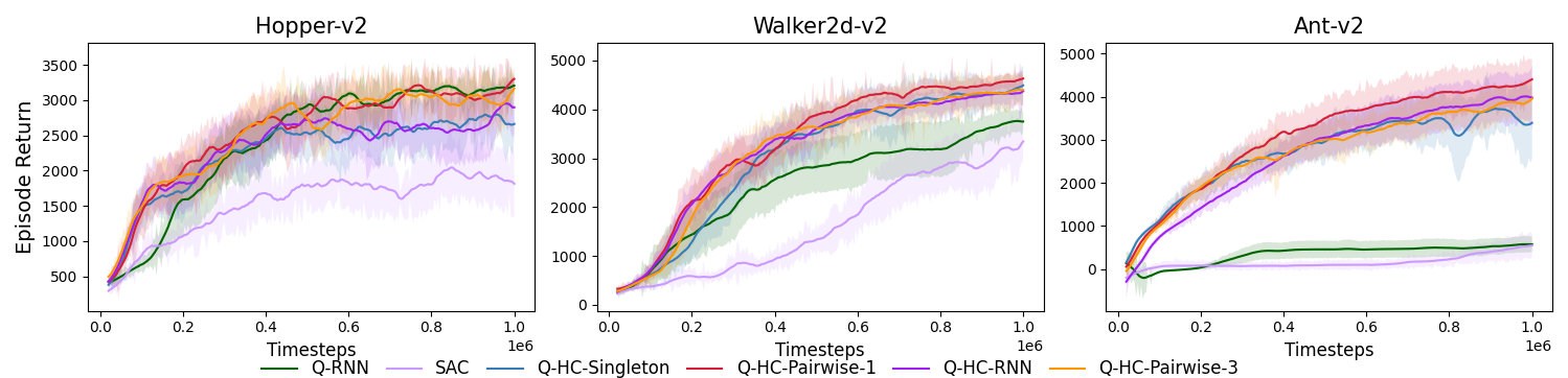
(a) Performance on High-Dimensional Tasks

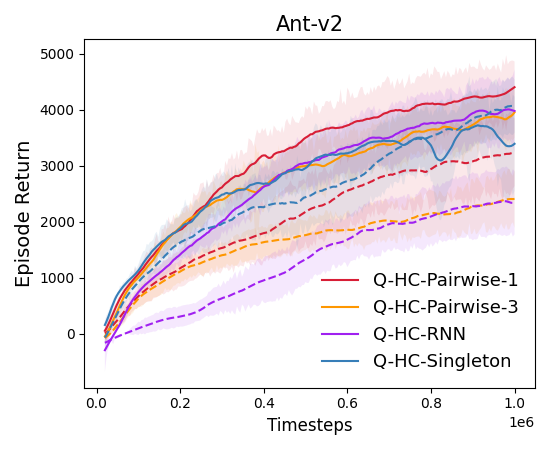
(b) Ablation on Regulation

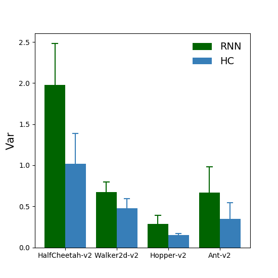
(c) Gradient Variance

Figure 1: (a): Performance of different implementations of HC-decomposition framework (${\mathcal{Q}}$-HC), ${\mathcal{Q}}$-RNN without HC-decomposition and vanilla SAC. The task is the continuous sum-form PI-DRMDP task. Reward function is the sum of standard per-step reward in these tasks. $q_{n}$ is a uniform distribution between 15 and 20. The results show the mean and standard deviation of 7 seeds each. (b) Ablation on the $L_{\text{reg}}$. Each dashed line is the no-regulation version of the corresponding ${\mathcal{Q}}$-HC of the same color. (c) Estimated variance of the policy gradient throughout the training. Details are shown in Appendix D.

Comparing Eq. (7) with Eq. (5), we note that the gradient on the policy $\pi$ under HC-decomposition will not be effected by $\tau_{t_{i}:t}$. Thus, for a mini-batch update, our policy gradient has less variance and the training becomes more efficient. In Figure 1(c), we visualize and compare the scale of the gradient variance of our HC-decomposition framework and the straightforward recurrent network approximation of the $\mathcal{Q}$ function, w.r.t. the same policy and the same batch of samples. Clearly, the result supports our claim that HC-decomposition results in less gradient variance.

Finally, to learn the $H_{\phi}$ and $C_{\phi}$ functions, we minimize the following objective function

$$\mathcal{L}^{\textsc{HC}}_{\phi}= \mathbb{E}_{D}[(R_{t}+\gamma(\hat{H}_{\phi}(\tau_{t_{i}:t+1})+\hat{C}_{\phi}(s_{t+1},a_{t+1}^{\prime}))-(H_{\phi}(\tau_{t_{i}:t})+C_{\phi}(s_{t},a_{t})))^{2}]+\lambda L_{\text{reg}}(H_{\phi}),$$ (8)

where the first term is the TD error in Eq. (4) and the second term is a regularizer on $H_{\phi}$. We use the regularization to stabilize the optimization process and prevent $H_{\phi}$ from taking away too much information of the credit on the choice of $a_{t}$. In practice, we may use different designs of $H_{\phi}$ and the regularization term based on domain knowledge or tasks’ properties. In Section 4, we will compare several simple choices of $H_{\phi}$ and $L_{\text{reg}}$. The search for other designs of $H_{\phi}$ and the regularization term in various settings is left as future work.

4 Experiment

In this section, we first test and illustrate our algorithmic framework and HC-decomposition on high-dimensional PI-DRMDP tasks to validate our claims in previous sections. Then, we compare our algorithm with several previous baselines on sum-form delayed reward tasks. Our algorithm turns out to be the SOTA algorithm which is most sample-efficient and stable. Finally, we demonstrate our algorithm via an illustrative example.

4.1 Design Evaluation

We implement the following architectures of $H_{\phi}$ in our experiment.

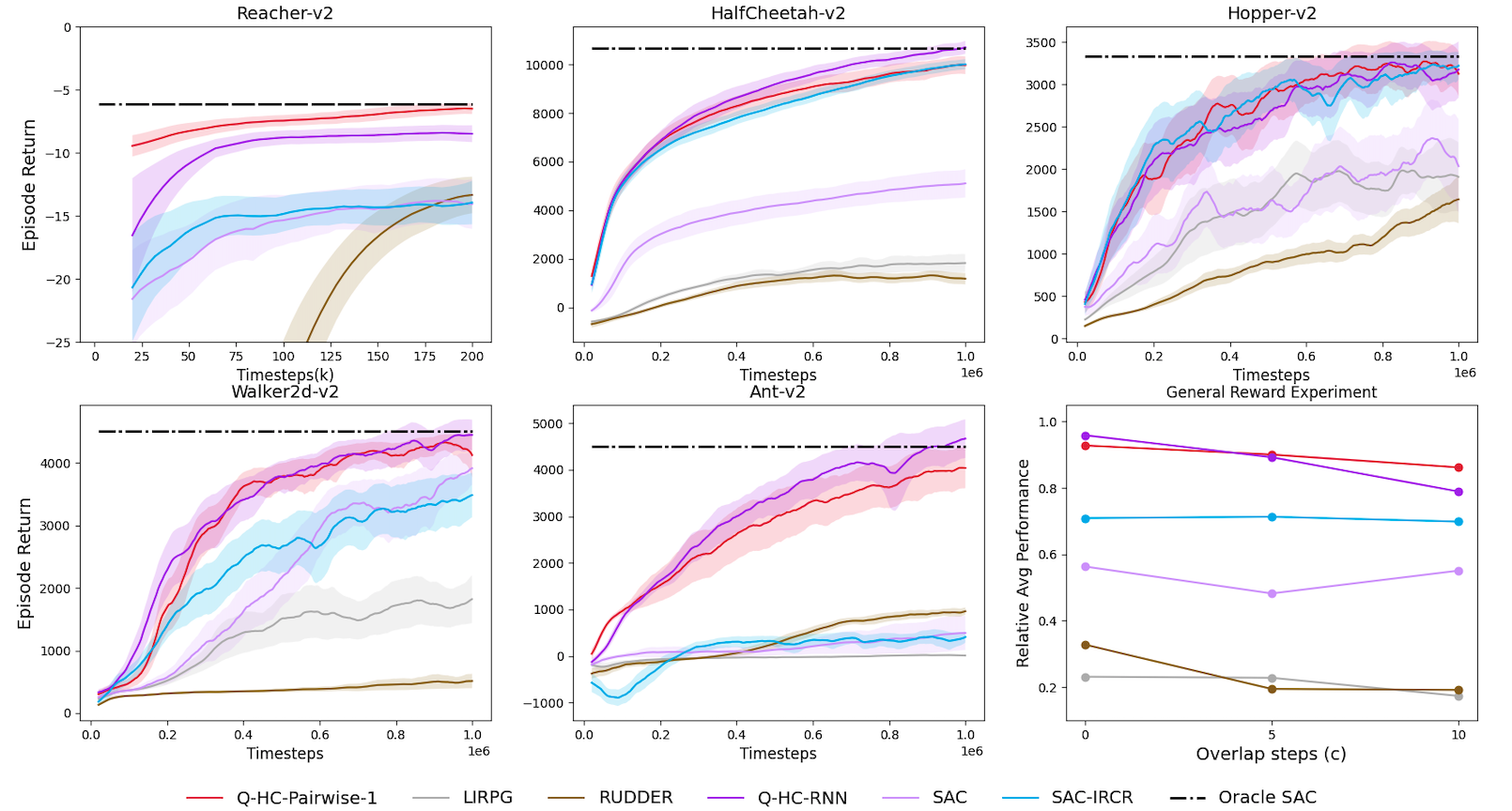
Figure 2: Comparisons of ${\mathcal{Q}}$-HC-Pairwise-1, ${\mathcal{Q}}$-HC-RNN and baselines on 5 sum-form PI-DRMDP  tasks. The dashed line is the value of Oracle SAC. $q_{n}$ is fixed as $20$ [10, 11]. The results show the mean and the standard deviation of 7 runs. All curves are further smoothed equally for clarity. The last picture shows the relative performance w.r.t the Oracle SAC on sum-form PI DRMDPtasks with General Reward Function ( Appendix A). Each data point shows the average of 5 tasks for each algorithm. X-axis refers to the overlapping steps of the reward function. Please refer to Appendix D for more details.

${\mathcal{Q}}$-HC-RNN. $H_{\phi}(\tau_{t_{i}:t})$ is approximated with a GRU network.

${\mathcal{Q}}$-HC-Pairwise-K. $H_{\phi}(\tau_{t_{i}:t})$ is the sum of $K$+$1$ networks $\{c^{k}_{\phi}\}_{k=0,1,\ldots K}$ for different pairwise terms as follows. $K=1,3$ are included in the experiment.

$$H_{\phi}(\tau_{t_{i}:t})= \sum_{k\in[0:K+1]}\sum_{j\in[t_{i}:t-k]}c_{\phi}^{k}(\tau_{j:j+1}\circ\tau_{j+k:j+k+1}).$$

${\mathcal{Q}}$-HC-Singleton. $H_{\phi}(\tau_{t_{i}:t})$ is the sum of single step terms.

$$H_{\phi}(\tau_{t_{i}:t})=\sum_{j\in[t_{i}:t]}b_{\phi}(\tau_{j:j+1}).$$

In terms of the representation power of these structures, (-RNN) is larger than (-Pairwise) larger than (-Singleton). With a small representation power, critic’s learning will suffer from large projection error. In terms of optimization, (-Singleton) is easier than (-Pairwise) and easier than (-RNN). As discussed in Section 3.2, non-optimized critic will result in inaccurate and unstable policy gradients. The practical design of $H_{\phi}$ is a trade-off between the efficiency of optimization and the scale of projection error. For the regularizer in Eq. (8), we choose the following for all implementations.

$$L_{\text{reg}}(H_{\phi})=\mathbb{E}_{D}\left[(H_{\phi}(\tau_{i})-r(\tau_{i}))^{2}\right],$$ (9)

where $\tau_{i}$ is sampled from the $D$. As discussed in Section 3.2, the history part $H_{\phi}(\tau_{t_{i}:t})$ should only be used to infer the credit of $\tau_{t_{i}:t}$ within the signal interval $\tau_{i}$. However, without the regularization, the approximated $H_{\phi}$ may deprive too much information from $\mathcal{Q}_{\phi}$ than we have expected. Thus, in a direct manner, we regularize $H_{\phi}(\tau_{i})$ to the same value of $r(\tau_{i})$.

We compare these algorithms on sum-form PI-DRMDP continuous control tasks based on OpenAI Gym. Rewards are given once every $n$ steps which is uniformly distributed from $15$ to $20$. The reward is the sum of the standard per-step reward in these tasks. We also compare the above HC implementations with vanilla SAC and ${\mathcal{Q}}$-RNN whose ${\mathcal{Q}}^{\pi}$ is approximated by a GRU network. All algorithms are based on SAC and we observe they outperform their TD3 variants in practice. Please refer to Appendix D for implementation details.

As shown in Figure 1(a), the empirical results validate our claims.

1. Algorithms under the algorithmic framework (i.e., with prefix ${\mathcal{Q}}$) outperform vanilla SAC. Our proposed method approximate ${\mathcal{Q}}^{\pi}$ in the algorithmic framework while vanilla SAC cannot handle non-Markovian rewards.

2. As tasks become more difficult, ${\mathcal{Q}}^{\pi}$ approximated with HC-decomposition architecture (i.e., with prefix ${\mathcal{Q}}$-HC) is more sample-efficient and more stable than ${\mathcal{Q}}$-RNN. Figure 1(c) demonstrates that HC-decomposition yields low gradient variance in policy updates as discussed in Section 3.2.

3. Figure 1(b) shows the importance of regularization, especially when $H_{\phi}$ has complex form (i.e., ${\mathcal{Q}}$-HC-RNN) and thus more likely to result in ill-optimized $C$-part.

4. We also find that ${\mathcal{Q}}$-HC-Pairwise-1 slightly outperforms other implementations in this environment. This indicates that it balances well between optimization efficiency and projection error on these tasks.

Additionally, we also conduct experiments on non-sum-form tasks based on OpenAI Gym in Appendix C. Results are still consistent with our analysis, i.e., methods with prefix ${\mathcal{Q}}$-HC outperform ${\mathcal{Q}}$-RNN and vanilla SAC. Thus, we believe the benefit of HC-decomposition architecture worth the potential defect of projection error. In future work, we will conduct more study on this architecture to understand its properties thoroughly.

4.2 Comparative Evaluation

In this subsection, we compare our algorithm with previous algorithms in sum-form  high-dimensional delayed reward tasks. The following baselines are included in the comparison.

• LIRPG [10]. It utilizes intrinsic rewards to make policy gradients more efficient. The intrinsic reward is learnt by meta-gradient from the same objective function. We use the same code provided by the paper.

• RUDDER [18]. It decomposes the delayed and sparse reward to a surrogate per-step reward via regression. Additionally, it utilizes on-policy correction to ensure the same optimality w.r.t the original problem. We alter the code for the locomotion tasks.

• SAC-IRCR [9]. It utilizes off-policy data to provide a smoothed guidance rewards for SAC. As mentioned in the paper, the performance heavily relies on the smoothing policy. We implement a delayed reward version of IRCR in our setting.

For clarity, we only include ${\mathcal{Q}}$-HC-Pairwise-1 and ${\mathcal{Q}}$-HC-RNN in the comparison. Results are shown in Figure 2. We find that LIRPG and RUDDER perform sluggishly in all tasks, perhaps due to the on-policy nature (i.e., based on PPO [19]). SAC-IRCR performs well only on some easy tasks (e.g. Hopper-v2). Unfortunately, in other cases, IRCR has a bad performance (e.g. Ant-v2, Walker2d-v2, Reacher-v2). We suspect in these tasks, the smoothing technique results in a misleading guidance reward which biases the agent. Thus, SAC-IRCR is not a safe algorithm in solving delay reward tasks. In contrast, ours as well as other implementations (shown in Appendix C) perform well on all tasks and surpass the baselines by a large margin. Most surprisingly, our algorithm can achieve the near optimal performance, i.e, comparing with Oracle SAC which is trained on dense reward environment for 1M steps. Noticing that we use an environment in which rewards are given only every 20 steps.

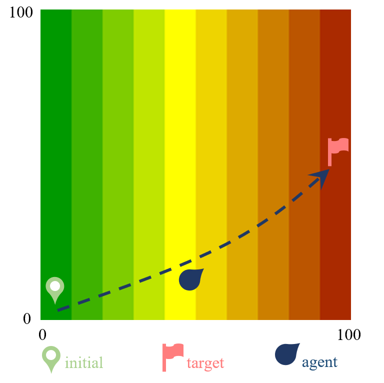
(a) Point Reach

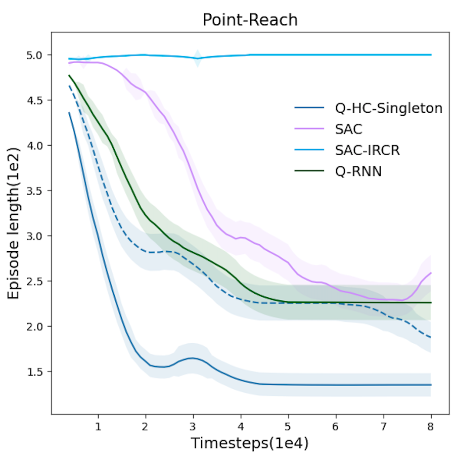
(b) Learning Curve

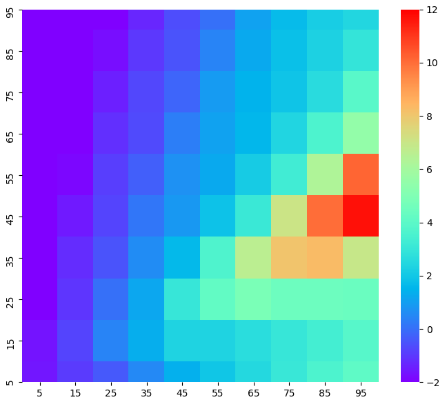
(c) Heatmap

Figure 3: (a) $100\times 100$ Point-Reach task with additional positional reward (indicated by area color). Reward is given every 20 steps. (b) Learning curves of ${\mathcal{Q}}$-HC-Singleton and several baselines. Dashed line represents ${\mathcal{Q}}$-HC-Singleton without regularization. Y-axis shows the number of steps needed for the point agent to reach the target area (cut after 500 steps). All curves represent the mean of 10 seeds and are smoothed equally for clarity.(c) Heatmap visualization of $b_{\phi}$ in ${\mathcal{Q}}$-HC-Singleton.

We also conduct experiments on tasks with general reward functions, in which algorithmic framework and the HC-decomposition can be naturally extended to (please refer to Appendix A and Appendix B). In the General Experiment of Figure 2, we plot the relative average performance w.r.t Oracle SAC for different amount of overlapped steps. ${\mathcal{Q}}$-HC is the SOTA algorithm in every circumstance. Please refer to Appendix D for experiment details.

4.3 Historical Information

In addition, with a toy example, we explore what kind of information the H-component learns so that the C-component makes suitable decisions. The toy example is a target-reaching task illustrated in Figure 3(a). The point agent is given delayed reward which roughly indicates its distance to the target area. This mimics the low frequency feedback from the environment. Noticing that the reward function is not in sum-form. Please refer to Appendix D for more details.

The learning curves are shown in Figure 3(b). Clearly, ${\mathcal{Q}}$-HC-Singleton outperforms the baselines by a large margin. For better illustration, we visualize $b_{\phi}(s_{t},a_{t})$ in ${\mathcal{Q}}$-HC-Singleton on the grid in Figure 3(c). The pattern highlights the line from the start point to the target area (i.e., the optimal policy), suggesting that $b_{\phi}$ has captured some meaningful patterns to boost training. We also observe a similar pattern for HC-Singleton without regression (Appendix D). This is an interesting discovery which shows that the H-component may also possess direct impact on the policy learning instead of simply function as an approximator.

5 Related Work

Off-Policy RL: Off-policy deep reinforcement learning algorithms TD3 [14] and SAC [13] are the most widely accepted actor-critic algorithms on the robot locomotion benchmark [20] so far. Based on previous work [21, 22], Fujimoto et al. [14] puts forward the clipped double Q-learning (CDQ) technique to address overestimation in critic learning. Haarnoja et al. [13] also uses CDQ technique but instead optimizes the maximum entropy objective. These two methods lead to a more robust policy. In our setting, we observe that SAC-based algorithms slightly outperforms TD3-based algorithms suggesting the benefit of maximum entropy in delayed reward tasks.

Delayed or Episodic Reward RL: Developing RL algorithms for delayed reward or episodic reward (at the end of the trajectory) has become a popular research area recently. These tasks are known to be difficult for long-horizon credit assignment [23]. To address this issue, Zheng et al. [10] proposes to use intrinsic reward to boost the efficiency of policy gradients. The intrinsic reward is learnt via meta-learning [24]. Gangwani et al. [25] and Guo et al. [26] use a discriminator to provide guidance reward for the policy. The discriminator is trained jointly with the policy with binary classification loss for self-imitating. In RUDDER [18], it utilizes a recurrent network to predict a surrogate per-step reward for guidance. To ensure the same optimality, the guidance is then corrected with ground truth reward. Liu et al. [27] extends the design and utilizes a Transformer [28] network for better credit assignment on episodic reward tasks. Recently, Klissarov and Precup [12] proposes to use GCN [29] network to learn a potential function for reward shaping [30]. Noticing that all these algorithms are based on PPO [19] and thus are on-policy algorithms while ours is an off-policy one.

Most recently, Gangwani et al. [9] proposes to augment off-policy algorithms with a trajectory-space smoothed reward in episodic reward setting. The design turns out to be effective in solving the problem. However, as mentioned by the paper itself, this technique lacks theoretical guarantee and heavily relies the choice of the smoothing policy. As shown in Section 4.2, in many cases, this method becomes extremely spurious. Our algorithm is derived from a theoretical perspective and performs well on all tasks.

6 Conclusion

In this paper, we model the sequential decision problem with delayed rewards as Past-Invariant Delayed Reward MDPs. As previous off-policy RL algorithms suffer from multiple problems in PI-DRMDP, we put forward a novel and general algorithmic framework to solve the PI-DRMDP problems that has theoretical guarantees in the tabular case. The framework relies on a novelly defined $\mathcal{Q}$-value. However, in high dimensional tasks, it is hard to approximate the $\mathcal{Q}$-value directly. To address this issue, we propose to use the HC-approximation framework for stable and efficient training in practice. In the experiment, we compare different implementations of the HC framework. They all perform well and robustly in continuous control PI-DRMDP locomotion tasks based on OpenAI Gym. Besides, our method outperforms previous baselines on delayed reward tasks remarkably, suggesting that our algorithm is a SOTA algorithm on these tasks so far.

In terms of future work, two research directions are worth exploring. One is to develop our algorithm and the HC-approximation scheme to various real world settings mentioned in Section 1. Additionally, we may also develop an offline [31] version of our algorithm which is more practically useful. The other direction is to design efficient and advanced algorithms with theoretical guarantees for the general DRMDP tasks.

Appendix A Discussions and Formal Proofs

In this part, we provide the proofs for the statements in the main paper. In addition, we also add detailed discussions on the issues mentioned above. To begin with, we restate the definitions with general reward functions.

Definition 3 (DRMDP with General Reward Function, DRMDP-c).

A DRMDP-$c$ $M_{c}=(S,A,p,q_{n},r_{c},\gamma)$ is described by the following parameters.

1. The state and action spaces are $S$ and $A$ respectively.

2. The Markov transition function is $p(s^{\prime}|s,a)$ for each $(s,a)\in S\times A$; the initial state distribution is $p(s_{0})$.

3. The signal interval length is distributed according to $q_{n}(\cdot)$, i.e., for the $i$-th signal interval, its length $n_{i}$ is independently drawn from $q_{n}(\cdot)$.

4. The general reward function $r_{c}$ defines the expected reward generated for each signal interval with a overlap of maximal $c$ steps with previous signal intervals; suppose $\tau_{i}=\tau_{t:t+n_{i}}=(s,a)_{t:t+n_{i}}=((s_{t},a_{t}),\dots(s_{t+n-1},a_{t+n_{i}-1}))$ is the state-action sequence during the $i$-th signal interval of length $n_{i}$, then the expected reward for this interval is $r_{c}(\tau_{t-c:t+n_{i}})$.

5. The reward discount factor is $\gamma$.

The PI-DRMDP is also extended naturally as following.

Definition 4 (PI-DRMDP with General Reward Function, PI-DRMDP-c).

A Past-Invariant DRMDP-$c$ is a DRMDP-$c$  $M_{c}=(S,A,p,q_{n},r_{c},\gamma)$ whose reward function $r_{c}$ satisfies the following Past-Invariant (PI) condition: for any two trajectory segments $\tau_{1}$ and $\tau_{2}$ of the same length (no less than $c$), and for any two equal-length trajectory segments $\tau_{1}^{\prime}$ and $\tau_{2}^{\prime}$ such that the concatenated trajectories $\tau_{a}\circ\tau_{b}^{\prime}$ are feasible under the transition dynamics $p$ for all $a,b\in\{1,2\}$, it holds that

$$r(\tau_{1}\circ\tau_{1}^{\prime})>r(\tau_{1}\circ\tau_{2}^{\prime})\iff r(\tau_{2}\circ\tau_{1}^{\prime})>r(\tau_{2}\circ\tau_{2}^{\prime}).$$

Remark 1.

Definition 1 and Definition 2 are the special case ($c=0$) of Definition 3 and Definition 4 respectively.

Clearly, we have the following Fact.

Fact 4.

$\forall c^{\prime}<c$, DRMDP $M_{c^{\prime}}$ is also a DRMDP $M_{c}$ and PI-DRMDP $M_{c^{\prime}}$ is also a PI-DRMDP $M_{c}$.

Besides, under the general reward function, we extend the ${\mathcal{Q}}$ definition.

$$\mathcal{Q}^{\pi}(\tau_{t_{i}-c:t+1}):=\mathbb{E}_{(\tau,n)\sim\pi}\left[\sum_{j=i}^{\infty}\gamma^{t_{j+1}-t-1}r(\tau_{t_{j}-c:t_{j+1}})\Big{|}\tau_{t_{i}-c:t+1}\right].$$ (10)

Correspondingly, ${\mathcal{Q}}^{\pi}(\tau_{t_{i}-c:t+1})$ is optimized via

$$\mathcal{L}_{\phi}:=\mathbb{E}_{D}\left[(R_{t}+\gamma\hat{\mathcal{Q}}_{\phi}(\tau_{t_{j}-c:t+2})-\mathcal{Q}_{\phi}(\tau_{t_{i}-c:t+1}))^{2}\right],$$ (11)

where $\tau_{t_{j}-c:t+2}=\tau_{t_{i}-c:t+1}\circ(s_{t+1},a^{\prime}_{t+1})$ (so that $j=i$) if $t$ is not the last step of $\tau_{i}$, and $\tau_{t_{j}-c:t+2}=\tau_{t_{i+1}-c:t_{i+1}}\circ(s_{t_{i+1}},a^{\prime}_{t_{i+1}})$ (so that $j=i+1$) otherwise.

The general policy update is also extended to

$$\nabla_{\theta}{\mathcal{J}}(\pi_{\theta})=\mathbb{E}_{D}\left[\nabla_{a_{t}}\mathcal{Q}^{\pi}(\tau_{t_{i}-c:t}\circ(s_{t},a_{t}))\Big{|}_{\pi_{\theta}(s_{t},t-t_{i})}\nabla_{\theta}\pi_{\theta}(s_{t},t-t_{i})\right].$$ (12)

Without specification, the following proofs hold for $\forall c$.

A.1 Proof of Fact 1

Under Definition 3, we denote $\Pi_{\tau,c}=\{\pi(a_{t}|\tau_{t_{i}-c:t}\circ s_{t})\}$ as the extension of $\Pi_{\tau}$ ($c=0$). Similarly, we restate the Fact 1 with general reward function as Fact 5.

Fact 5 (Fact 1 with General Reward Function).

For any DRMDP-$c$, there exists an optimal policy $\pi^{*}\in\Pi_{\tau,c}$. However, there exists some DRMDP-$0$ (so as DRMDP-c $\forall c$) such that all of its optimal policies $\pi^{*}\notin\Pi_{s}$.

In general, any policy belongs to the class $\Pi_{\text{all}}=\{\pi(a_{t}|\tau_{0:t}\circ s_{t},n_{0:t})\}$. Namely, the agent’s policy can only base on all the information it has experienced till step $t$. Besides, in DRMDP-c, the expected discounted cumulative reward is

$${\mathcal{J}}(\pi)=\sum_{\tau,n}\rho^{\pi}(\tau,n)R(\tau,n).$$

where $\rho^{\pi}(\tau,n)$ denotes the probability that trajectory ($\tau,n$) is generated under policy $\pi\in\Pi_{\text{all}}$. To begin with, we first prove the following Lemma.

Lemma 1.

For any policy $\pi\in\Pi_{\text{all}}$ which is the optimal, i.e, maximize ${\mathcal{J}}(\pi)$, we consider two segments of trajectories $(\tau_{0:t^{a}}^{a},n_{0:t^{a}}^{a})$ and $(\tau_{0:t^{b}}^{b},n_{0:t^{b}}^{b})$ which satisfies that $\tau^{a}_{t^{a}_{i}-c:t^{a}}=\tau^{b}_{t^{b}_{i}-c:t^{b}}$ and $t^{b}\geq t^{a}$. Besides, we also consider $\forall t\geq t^{b},t^{\prime}=t-t^{b}+t^{a}$ and $\tau^{b}_{0:t}=\tau^{b}_{0:t^{b}}\circ\tau_{t^{b}:t},n^{b}_{0:t}=n^{b}_{0:t^{b}}\circ n_{t^{b}:t}$ and state $s_{t}^{(^{\prime})}$ feasible in the dynamic, we switch the policy $\pi$ to $\pi^{\prime}$ w.r.t these two trajectories as following

$$\pi^{\prime}(\cdot|\tau^{b}_{0:t}\circ s_{t},n^{b}_{0:t})=\pi(\cdot|\tau^{a}_{0:t^{a}}\circ\tau_{t^{b}:t}\circ s_{t^{\prime}},n^{a}_{0:t^{a}}\circ n_{t^{b}:t}).$$

Then, $\pi^{\prime}\in\Pi_{\text{all}}$ and ${\mathcal{J}}(\pi^{\prime})={\mathcal{J}}(\pi)$.

Proof.

Obviously, $\pi^{\prime}$ is well-defined and $\pi^{\prime}\in\Pi_{\text{all}}$ as the transition is Markovian. Noticing that

$${\mathcal{J}}(\pi^{\prime}) =\sum_{\tau,n}\rho^{\pi^{\prime}}(\tau,n)R(\tau,n)$$

$$=\underbrace{\sum_{(\tau,n):(\tau^{b}_{0:t^{b}},n^{b}_{0:t^{b}})\not\subset(\tau,n)}\rho^{\pi^{\prime}}(\tau,n)R(\tau,n)}_{\text{denoted by }J^{\pi^{\prime}}(\tau_{0:t^{b}}^{b},n_{0:t^{b}}^{b})}+\rho^{\pi^{\prime}}(\tau^{b}_{0:t^{b}},n^{b}_{0:t^{b}})\sum_{(\tau,n):(\tau^{b}_{0:t^{b}},n^{b}_{0:t^{b}})\subset(\tau,n)}\rho^{\pi^{\prime}}(\tau,n|\tau_{0:t^{b}}^{b},n_{0:t^{b}}^{b})R(\tau,n)$$

$$=J^{\pi^{\prime}}(\tau^{b}_{0:t^{b}},n^{b}_{0:t^{b}})+\rho^{\pi^{\prime}}(\tau^{b}_{0:t^{b}},n^{b}_{0:t^{b}})\sum_{(\tau,n):(\tau^{b}_{0:t^{b}},n^{b}_{0:t^{b}})\subset(\tau,n)}\rho^{\pi^{\prime}}(\tau,n|\tau_{0:t^{b}}^{b},n_{0:t^{b}}^{b})\left(\sum_{j=1}^{\infty}\gamma^{t_{j+1}-1}r(\tau_{t_{j}-c:t_{j+1}})\right)$$

$$=J^{\pi^{\prime}}(\tau^{b}_{0:t^{b}},n^{b}_{0:t^{b}})+\rho^{\pi^{\prime}}(\tau^{b}_{0:t^{b}},n^{b}_{0:t^{b}})\left(\sum_{j=1}^{i(t^{b})-1}\gamma^{t_{j+1}-1}r(\tau_{t_{j}-c:t_{j+1}})\right)+\rho^{\pi^{\prime}}(\tau^{b}_{0:t^{b}},n^{b}_{0:t^{b}})\left(\gamma^{t^{b}-1}{\mathcal{Q}}^{\pi^{\prime}}(\tau^{b}_{t_{i}^{b}-c:t^{b}})\right).$$

We denote $(\tau_{0:t},n_{0:t})\subset(\tau,n)$ if the former is the trajectory prefix of the latter. ${\mathcal{Q}}^{\pi^{\prime}}$ is defined in Eq. (3) except that $\pi^{\prime}\in\Pi_{\text{all}}$ in this case. By the definition of $\pi^{\prime}$ and the condition that $\pi$ is optimal, we have ${\mathcal{Q}}^{\pi^{\prime}}(\tau_{t_{i}^{b}-c:t^{b}}^{b})={\mathcal{Q}}^{\pi}(\tau_{t_{i}^{a}-c:t^{a}}^{a})={\mathcal{Q}}^{\pi}(\tau_{t_{i}^{b}-c:t^{b}}^{b})$ and $J^{\pi^{\prime}}(\tau^{b}_{0:t^{b}},n^{b}_{0:t^{b}})=J^{\pi}(\tau^{b}_{0:t^{b}},n^{b}_{0:t^{b}})$. Thus, we have

$${\mathcal{J}}(\pi^{\prime}) =J^{\pi^{\prime}}(\tau^{b}_{0:t^{b}},n^{b}_{0:t^{b}})+\rho^{\pi^{\prime}}(\tau^{b}_{0:t^{b}},n^{b}_{0:t^{b}})\left(\sum_{j=1}^{i(t^{b})-1}\gamma^{t_{j+1}-1}r(\tau_{t_{j}-c:t_{j+1}})\right)+\rho^{\pi^{\prime}}(\tau^{b}_{0:t^{b}},n^{b}_{0:t^{b}})\left(\gamma^{t^{b}-1}{\mathcal{Q}}^{\pi}(\tau^{b}_{t_{i}^{b}-c:t^{b}})\right)$$

$$=J^{\pi}(\tau^{b}_{0:t^{b}},n^{b}_{0:t^{b}})+\rho^{\pi}(\tau^{b}_{0:t^{b}},n^{b}_{0:t^{b}})\sum_{(\tau,n):(\tau^{b}_{0:t^{b}},n^{b}_{0:t^{b}})\subset(\tau,n)}\rho^{\pi}(\tau,n|\tau_{0:t^{b}}^{b},n_{0:t^{b}}^{b})\left(\sum_{j=1}^{\infty}\gamma^{t_{j+1}-1}r(\tau_{t_{j}-c:t_{j+1}})\right)$$

$$={\mathcal{J}}(\pi).$$

∎

We refer it as a policy switch on $\pi$ w.r.t $(\tau_{0:t^{b}}^{b},n_{0:t^{b}}^{b})$ and $(\tau_{0:t^{a}}^{a},n_{0:t^{a}}^{a})$ to $\pi^{\prime}$. Then, we prove Fact 5 as follows.

Proof of Fact 5.

For simplicity, we denote $\Pi_{\tau,c}^{t}\subset\Pi_{\text{all}}$ as the policy space that if $\pi\in\Pi_{\tau,c}^{t}$ and $\forall t_{a},t_{b}\leq t$ then $\forall(\tau_{0:t^{a}}^{a},n_{0:t^{a}}^{a}),(\tau_{0:t^{b}}^{b},n_{0:t^{b}}^{b})$ which $\tau^{a}_{t^{a}_{i}-c:t^{a}}=\tau^{b}_{t^{b}_{i}-c:t^{b}}$, $\pi(\cdot|\tau^{a}_{0:t^{a}}\circ s_{t^{a}},n^{a}_{0:t^{a}})=\pi(\cdot|\tau^{b}_{0:t^{b}}\circ s_{t^{b}},n^{b}_{0:t^{b}})$ for all $s$ feasible. Clearly, $\Pi_{\tau,c}^{0}=\Pi_{\text{all}}$ and $\Pi_{\tau,c}^{\infty}=\Pi_{\tau,c}$. Then, starting from some optimal policy $\pi_{0}\in\Pi_{\tau,c}^{0}$, we utilize the policy switch operation to shift it into $\Pi_{\tau}$.

Suppose that $\pi_{t-1}\in\Pi_{\tau,c}^{t-1}$, we consider the following two steps of operations.

1. Step 1. $\forall(\tau_{0:t},n_{0:t})$ that $\exists(\tau^{\prime}_{0:t^{\prime}},n^{\prime}_{t_{i}^{\prime}:t^{\prime}})$ which $t^{\prime}<t$ and $\tau_{t_{i}-c:t}=\tau^{\prime}_{t_{i}^{\prime}-c:t^{\prime}}$ (randomly choose one if multiple segments exist), we conduct a policy switch on $\pi_{t}$ w.r.t $(\tau_{0:t},n_{0:t})$ and $(\tau_{0:t^{\prime}},n_{0:t^{\prime}})$. We denote the policy after all these policy switches as $\pi_{t-1}^{\prime}$.

2. Step 2. We denote $S_{\pi_{t-1}}(\tilde{\tau}_{t_{i}-c:t})=\{(\tau_{0:t},n_{0:t})|\tau_{t_{i}-c:t}=\tilde{\tau}_{t_{i}-c:t}\text{ and }\nexists(\tau^{\prime}_{0:t^{\prime}},n^{\prime}_{0:t^{\prime}}),t^{\prime}<t\text{ which }\tau^{\prime}_{t_{i}^{\prime}-c:t^{\prime}}=\tilde{\tau}_{t_{i}-c:t}\}$. For each $S_{\pi_{t-1}}(\tilde{\tau}_{t_{i}-c:t})$, we randomly choose some $(\tau_{0:t}^{0},n_{0:t}^{0})\in S_{\pi_{t-1}}(\tilde{\tau}_{t_{i}-c:t})$ and conduct policy switch on $\pi^{\prime}_{t-1}$ w.r.t all $(\tau,n)\in S_{\pi_{t-1}}(\tilde{\tau}_{t_{i}-c:t})$ and $(\tau_{0:t}^{0},n_{0:t}^{0})$. Finally, we get $\pi_{t}$.

Since $\pi_{t-1}\in\Pi_{\tau,c}^{t-1}$, it is straightforward to check that $\pi_{t}\in\Pi_{\tau,c}^{t}$. Besides, as all operations are policy switches, $\pi_{t}$ is optimal if $\pi_{t-1}$ is optimal. Consequently, by induction from the optimal policy $\pi_{0}$, we can prove that $\exists\pi_{\infty}\in\Pi_{\tau,c}$ which is optimal.

For the second statement, we consider the following DRMDP-0.

whose $n=2$. $a_{0},a_{1}$ denote two actions from $A_{0},A_{1}$ to $B$ respectively and $b_{0},b_{1}$ are two actions from B to C. The reward is defined as $r(a_{i},b_{j})=i\oplus j,\forall(i,j)\in\{0,1\}$. The initial state distribution is $p(A_{0})=p(A_{1})=0.5$. Clearly, for any optimal policy, the agent has to query for its action from the initial state to B before deciding the action from B to C. This illustrates that $\pi^{*}$ may not be in $\Pi_{s}$. ∎

Remark 2.

Fact 1 holds as the special case of Fact 5 when $c=0$.

A.2 Proof of Fact 2

Fact 6 (Fact 2 with General Reward Function).

For any distribution $D$ with non-zero measure for any $\tau_{t_{i}-c:t+1}$, $\mathcal{Q}^{\pi}(\tau_{t_{i}-c:t+1})$ is the unique fixed point of the MSE problem in Eq. (4). More specifically, when fixing $\hat{\mathcal{Q}}_{\phi}$ as the corresponding $\mathcal{Q}^{\pi}$, the solution of the MSE problem is still $\mathcal{Q}^{\pi}$.

Proof.

Though we state the fact for PI-DRMDP-c, we will prove it for general $\pi\in\Pi_{\tau,c}$ in DRMDP-c setting. For brevity, we replace $t+1$ with $t$ in the proof. By definition in Eq. (10), we have

$${\mathcal{Q}}^{\pi}(\tau_{t_{i}-c:t})= \leavevmode\nobreak\ q_{n}(n_{i}\neq t-t_{i}|n_{i}\geq t-t_{i})\left(\gamma\sum_{s_{t},a_{t}}p(s_{t}|s_{t-1},a_{t-1})\pi(a_{t}|\tau_{t_{i}-c:t}\circ s_{t}){\mathcal{Q}}^{\pi}(\tau_{t_{i}-c:t}\circ(s_{t},a_{t}))\right)$$

$$+q_{n} (n_{i}=t-t_{i}|n_{i}\geq t-t_{i})\left(r(\tau_{t_{i}-c:t})+\gamma\sum_{s_{t},a_{t}}p(s_{t}|s_{t-1},a_{t-1})\pi(a_{t}|\tau_{t-c:t}\circ s_{t}){\mathcal{Q}}^{\pi}(\tau_{t-c:t}\circ(s_{t},a_{t}))\right).$$ (13)

Clearly, ${\mathcal{Q}}^{\pi}(\tau_{t_{i}-c:t})$ is the solution of the following MSE problem. Noticing that we assume ${\mathcal{Q}}_{\phi}$ has tabular expression over $\tau_{t_{i}-c:t}$s.

$$\min_{\phi}\sum_{R_{t-1},s_{t}}p_{D}(\tau_{t_{i}-c:t},R_{t-1},s_{t})\pi(a_{t}^{\prime}|\tau_{t_{j}-c:t}\circ s_{t})\left(R_{t-1}+\gamma{\mathcal{Q}}^{\pi}(\tau_{t_{j}-c:t}\circ(s_{t},a_{t}^{\prime}))-{\mathcal{Q}}_{\phi}(\tau_{t_{i}-c:t})\right)^{2}.$$

Here, $\tau_{t_{j}-c:t}$ is defined similarly as in the main text and $p_{D}$ refers to the probability of the fragment of trajectory is sampled from the buffer $D$. We denote the objective function as ${\mathcal{L}}_{\phi}(\tau_{t_{i}-c:t})$. As ${\mathcal{L}}_{\phi}$ in Eq. (11) is the sum of all ${\mathcal{L}}_{\phi}(\tau_{t_{i}-c:t})$, ${\mathcal{Q}}^{\pi}(\tau_{t_{i}-c:t})$ is a fixed point of the MSE problem.

The uniqueness is proved similar to the standard MDPs setting. For any $\hat{{\mathcal{Q}}}_{\phi}$, we denote the optimal solution of Eq. (4) as ${\mathcal{Q}}_{\phi}(\tau_{t_{i}-c:t})$. Since we assume tabular expression and non-zero probability of any $p_{D}(\tau_{t_{i}-c:t})$ Then, $\forall\tau_{t_{i}-c:t}$, we have

$$\Big{|}{\mathcal{Q}}_{\phi}(\tau_{t_{i}-c:t})-{\mathcal{Q}}^{\pi}(\tau_{t_{i}-c:t})\Big{|}\leq \leavevmode\nobreak\ \gamma q_{n}(n_{i}\neq t-t_{i}|n_{i}\geq t-t_{i})\sum_{s_{t},a_{t}}p(s_{t}|s_{t-1},a_{t-1})\pi(a_{t}|\tau_{t_{i}-c:t}\circ s_{t})\Big{|}\hat{{\mathcal{Q}}}_{\phi}(\tau_{t_{i}-c:t+1})-$$

$${\mathcal{Q}}^{\pi}(\tau_{t_{i}-c:t+1})\Big{|}+\gamma q_{n}(n_{i}=t-t_{i}|n_{i}\geq t-t_{i})\sum_{s_{t},a_{t}}p(s_{t}|s_{t-1},a_{t-1})\pi(a_{t}|\tau_{t-c:t}\circ s_{t})$$

$$\Big{|}\hat{{\mathcal{Q}}}_{\phi}(\tau_{t-c:t}\circ(s_{t},a_{t}))-{\mathcal{Q}}^{\pi}(\tau_{t-c:t}\circ(s_{t},a_{t}))\Big{|}$$

$$\leq \leavevmode\nobreak\ \leavevmode\nobreak\ \gamma\parallel\hat{{\mathcal{Q}}}_{\phi}-{\mathcal{Q}}^{\pi}\parallel_{\infty}$$

Last term denotes the infinite norm of the vector of residual value between ${\mathcal{Q}}^{\pi}$ and $\hat{{\mathcal{Q}}}_{\phi}$. Each entry corresponds to some $\tau_{t_{i}-c:t}$ feasible in the dynamic. Consequently, by the $\gamma$-concentration property, if ${\mathcal{Q}}_{\phi}=\hat{{\mathcal{Q}}}_{\phi}$ after the iteration (i.e., ${\mathcal{Q}}_{\phi}$ is a fixed point), then ${\mathcal{Q}}_{\phi}={\mathcal{Q}}^{\pi}$. This completes the proof of uniqueness. ∎

Remark 3.

Fact 2 holds as the special case of Fact 6 when $c=0$.

A.3 Proof of Fact 3

Fact 7 (Fact 3 with General Reward Function).

For any $\tau_{t_{i}-c:t},\tau_{t_{i}-c:t}^{\prime}$ and $s_{t},a_{t},a_{t}^{\prime}$ which both $\tau_{t_{i}-c:t}\circ s_{t}$ and $\tau_{t_{i}-c:t}^{\prime}\circ s_{t}$ are feasible under the transition dynamics, $\forall\pi\in\Pi_{s}$, we have that

$$\mathcal{Q}^{\pi}(\tau_{t_{i}-c:t}\circ(s_{t},a_{t}))>\mathcal{Q}^{\pi}(\tau_{t_{i}-c:t}\circ(s_{t},a_{t}^{\prime}))\iff\mathcal{Q}^{\pi}(\tau_{t_{i}-c:t}^{\prime}\circ(s_{t},a_{t}))>\mathcal{Q}^{\pi}(\tau_{t_{i}-c:t}^{\prime}\circ(s_{t},a_{t}^{\prime}))$$

Proof.

Since $\pi(a_{t}|s_{t},t-t_{i})\in\Pi_{s}$, for any $s_{t},a_{t}$, the distribution of the remaining trajectories $\rho^{\pi}(\tau_{t:T},n_{t:T}|s_{t},a_{t},t_{i})$ is irrelevant with $\tau_{t_{i}-c:t}$ . Thus, we have

$${\mathcal{Q}}^{\pi}(\tau_{t_{i}-c:t}\circ(s_{t},a_{t}))= \sum_{\tau_{t:\infty},n_{t:\infty}}\rho^{\pi}(\tau_{t:\infty},n_{t:\infty}|s_{t},a_{t},t_{i})\left(\sum_{j=i}^{\infty}\gamma^{t_{j+1}-t-1}r(\tau_{t_{j}-c:t_{j+1}})\right)$$

$$= \sum_{t_{i+1}}\gamma^{t_{i+1}-t-1}q_{n}(n_{i}=t_{i+1}-t_{i}|n_{i}\geq t-t_{i})\sum_{\tau_{t:t_{i+1}}}\rho^{\pi}(\tau_{t:t_{i+1}}\circ s_{t_{i+1}}|s_{t},a_{t},t_{i})$$

$$\cdot\left(r(\tau_{t_{i}-c:t_{i+1}})+\gamma\sum_{a_{t_{i+1}}}\pi(a_{t_{i+1}}|s_{t_{i+1}},0){\mathcal{Q}}^{\pi}(\tau_{t_{i+1}-c:t_{i+1}}\circ(s_{t_{i+1}},a_{t_{i+1}}))\right)$$

$$\propto \sum_{t_{i+1},\tau_{t:t_{i+1}}}q_{n}(n_{i}=t_{i+1}-t_{i}|n_{i}\geq t-t_{i})\rho^{\pi}(\tau_{t:t_{i+1}}|s_{t},a_{t},t_{i})r(\tau_{t_{i}-c:t_{i+1}})+K(s_{t},a_{t},t_{i})$$

The last term denotes the residual part which is irrelevant with $\tau_{t_{i}:t}$. Besides, under the PI condition, the order of $r(\tau_{t_{i}-c:t_{i+1}})$ is invariant over $\tau_{t_{i}-c:t}$. As a result, the order of ${\mathcal{Q}}^{\pi}(\tau_{t_{i}-c:t}\circ(s_{t},a))$ among $a$ is also invariant of $\tau_{t_{i}-c:t}$. This completes the proof. ∎

Remark 4.

Fact 3 holds as then special case of Fact 7 when $c=0$.

A.4 Proof of Proposition 1

Proposition 2 (Proposition 1 with General Reward Function).

For any policy $\pi_{k}\in\Pi_{s}$, the policy iteration w.r.t. $\mathcal{Q}^{\pi_{k}}$ (Eq. (10)) produces policy $\pi_{k+1}\in\Pi_{s}$ such that $\forall\tau_{t_{i}-c:t+1}$, it holds that

$$\mathcal{Q}^{\pi_{k+1}}(\tau_{t_{i}-c:t+1})\geq\mathcal{Q}^{\pi_{k}}(\tau_{t_{i}-c:t+1}),$$

which implies that $\mathcal{J}(\pi_{k+1})\geq\mathcal{J}(\pi_{k})$.

Proof.

Under Fact 7, the new policy iteration is defined formally as following

$$\pi_{k+1}(a_{t}|s_{t},t-t_{i})=\operatorname*{arg\,max}_{a_{t}}{\mathcal{Q}}^{\pi_{k}}(\tau_{t-c:t}\circ(s_{t},a_{t}))$$

where $\tau_{t-c:t}$ is any trajectory segments feasible for $s_{t}$ under the dynamics. If there are multiple maximums, we can assign arbitrary probability among these $a_{t}$s. Following Eq. (13), we have $\forall\tau_{t_{i}-c:t}$

$${\mathcal{Q}}^{\pi_{k}}(\tau_{t_{i}-c:t}) =\leavevmode\nobreak\ q_{n}(n_{i}\neq t-t_{i}|n_{i}\geq t-t_{i})\left(\gamma\sum_{s_{t},a_{t}}p(s_{t}|s_{t-1},a_{t-1})\pi_{k}(a_{t}|s_{t},t-t_{i}){\mathcal{Q}}^{\pi_{k}}(\tau_{t_{i}-c:t}\circ(s_{t},a_{t}))\right)+$$

$$q_{n}(n_{i}=t-t_{i}|n_{i}\geq t-t_{i})\left(r(\tau_{t_{i}-c:t})+\gamma\sum_{s_{t},a_{t}}p(s_{t}|s_{t-1},a_{t-1})\pi_{k}(a_{t}|s_{t},0){\mathcal{Q}}^{\pi_{k}}(\tau_{t-c:t}\circ(s_{t},a_{t}))\right)$$

$$\leq\leavevmode\nobreak\ q_{n}(n_{i}\neq t-t_{i}|n_{i}\geq t-t_{i})\left(\gamma\sum_{s_{t},a_{t}}p(s_{t}|s_{t-1},a_{t-1})\pi_{k+1}(a_{t}|s_{t},t-t_{i}){\mathcal{Q}}^{\pi_{k}}(\tau_{t_{i}-c:t}\circ(s_{t},a_{t}))\right)+$$

$$q_{n}(n_{i}=t-t_{i}|n_{i}\geq t-t_{i})\left(r(\tau_{t_{i}-c:t})+\gamma\sum_{s_{t},a_{t}}p(s_{t}|s_{t-1},a_{t-1})\pi_{k+1}(a_{t}|s_{t},0){\mathcal{Q}}^{\pi_{k}}(\tau_{t-c:t}\circ(s_{t},a_{t}))\right)$$ (14)

Then, we can iteratively extend each ${\mathcal{Q}}^{\pi_{k}}$ term in Eq. (14) and get $\forall\tau_{t_{i}-c:t}$

$${\mathcal{Q}}^{\pi_{k}}(\tau_{t_{i}-c:t})\leq{\mathcal{Q}}^{\pi_{k+1}}(\tau_{t_{i}-c:t})$$

Noticing that the inequality is strict if any step of the inequality in the iterations is strict. Furthermore, by definition, ${\mathcal{J}}(\pi)=\sum_{s_{0},a_{0}}p(s_{0})\pi(a_{0}|s_{0},0){\mathcal{Q}}^{\pi}(s_{0},a_{0})$, we have

$${\mathcal{J}}(\pi_{k}) \leq\sum_{s_{0},a_{0}}p(s_{0})\pi_{k+1}(a_{0}|s_{0},0){\mathcal{Q}}^{\pi_{k}}(s_{0},a_{0})$$

$$\leq\sum_{s_{0},a_{0}}p(s_{0})\pi_{k+1}(a_{0}|s_{0},0){\mathcal{Q}}^{\pi_{k+1}}(s_{0},a_{0})$$

$$\leq{\mathcal{J}}(\pi_{k+1})$$

This completes the proof. ∎

Remark 5.

Proposition 1 holds as the special case of Proposition 2 when $c=0$.

A.5 Discussion of Off-Policy Bias

This following example illustrates the off-policy bias concretely. We consider the case for a sum-form PI-DRMDP-0.

The signal interval length is fixed as $n+1$ and any trajectory ends after one interval. The reward function is in sum-form over $r(s,a)$. When learning the critic (tabular expression) via Eq. (1), the $Q$-values at the last step $n$ are

$$Q_{\phi}(s_{n},a_{n})=\sum_{\tau_{0:n}}\rho^{\bm{\beta}}(\tau_{0:n}|s_{n},a_{n})r(\tau_{1})$$

$$=\underbrace{\sum_{\tau_{0:n}}\rho^{\bm{\beta}}(\tau_{0:n}|s_{n},a_{n})\left(\sum_{t=0}^{n-1}r(\tau_{t:t+1})\right)}_{\widetilde{Q^{\bm{\beta}}}(s_{n},a_{n})}+r(s_{n},a_{n})$$ (15)

In Eq. (15), $\rho^{\bm{\beta}}(\tau_{0:n}|s_{n},a_{n})$ denotes the probability distribution of $\tau_{0:n}$ collected under the policy sequence $\bm{\beta}$ conditioning on that $\tau_{n:n+1}=(s_{n},a_{n})$. Besides, we denote $\rho^{\beta_{k}}(\tau_{0:n}|s_{n})$ as the distribution under policy $\beta_{k}$ conditioning on $s_{n}$ at the last step. Obviously, $\rho^{\beta_{k}}$ is independent of last step’s action $a_{n}$ as $\pi\in\Pi_{s}$. By Bayes rule, we have the following relation

$$\rho^{\bm{\beta}}(\tau_{0:n}|s_{n},a_{n})=\frac{\sum_{k=1}^{K}\rho^{\beta_{k}}(\tau_{0:n}|s_{n})\beta_{k}(a_{n}|s_{n})}{\sum_{k=1}^{K}\beta_{k}(a_{n}|s_{n})}$$ (16)

In other word, $\rho^{\bm{\beta}}(\cdot|s_{n},a_{n})$ is a weighted sum of $\{\rho^{\beta_{k}}(\cdot|s_{n})\}$. The weights are different between $a_{n}$s since the behavior policies $\{\beta_{k}\}$ are different. Consequently, $\widetilde{Q^{\bm{\beta}}}(s_{n},a_{n})$ will also vary between $a_{n}$s and it is hard to be quantified in practice. Unfortunately, we may want $Q_{\phi}(s_{n},a_{n})\propto r(s_{n},a_{n})$ for unbiased credit assignment the actions at the last step. Thus, updating the policy with approximated $Q_{\phi}(s_{n},a_{n})$ will suffer from the off-policy bias term $\widetilde{Q^{\bm{\beta}}}(s_{n},a_{n})$.

A.6 Discussion of Fixed Point Bias

Even with on-policy samples in $D$, critic learning via Eq. (1) can still be erroneous. We formally state the observation via a toy sum-form PI-DRMDP-0.

where for state $B,C,D$, there is only one action. The agent only needs to decide among $a_{0},a_{1}$ at state $A$. $n$ is fixed as $2$ and the initial state distribution $p_{0}(A)=p_{0}(B)=0.5$. The reward has sum-form over the following per-step reward

$$r(C,c)=r(D,d)=0$$

$$r(A,a_{0})=0.01,r(A,a_{1})=1$$

$$r(B,b)=-1$$

Fact 8.

For the above PI-DRMDP-0 and any initialization of the policy, value evaluation ($Q_{\phi}(s_{t},a_{t})$ in tabular form) via Eq. (1) with on-policy data and policy iteration w.r.t $Q_{\phi}(s_{t},a_{t})$ will converge to a sub-optimal policy with ${\mathcal{J}}(\pi)=-0.495\gamma$. In contrast, our algorithm can achieve the optimal policy with ${\mathcal{J}}(\pi)=0$.

Proof.

For any policy $\pi$, we denote $p=\pi(a_{1}|A)$. Then, if we minimize Eq. (1) with on-policy samples, we will have $Q_{\phi}(C,c)=0.01,Q_{\phi}(A,a_{0})=0.01\gamma$. Besides, as initial state distribution are uniform, we have

$$Q_{\phi}(D,d)=\frac{1}{2}(p-1),\leavevmode\nobreak\ \leavevmode\nobreak\ Q_{\phi}(A,a_{1})=\frac{1}{2}\gamma(p-1)$$

Since $Q_{\phi}(A,a_{1})<Q_{\phi}(A,a_{0})$ for any $p$, policy iteration will converges to a sub-optimal policy that $\pi(a_{0}|A)=1$.The sub-optimal policy has ${\mathcal{J}}(\pi)=-0.495\gamma$. Noticing that this holds even if the initial policy is already the optimal.

For our algorithm, we have

$$Q_{\phi}(A,a_{1})=\gamma Q_{\phi}(A,a_{0},D,d)=\gamma$$

For any $\gamma>0$ and any $p$, a single policy iteration will have the optimal policy with but the optimal has ${\mathcal{J}}(\pi^{*})=0$. ∎

A.7 Discussion of Optimal Policy in PI-DRMDP

In our work on PI-DRMDP, we only focus on the optimization in $\Pi_{s}$. However, in some bizarre cases, the optimal policy $\pi^{*}\not\in\Pi_{s}$. For example, consider the following PI-DRMDP-0 where $n$ if fixed as 2.

The initial state is uniformly chosen from $\{A_{b},A_{l}\}$ and $C_{+},T$ are terminal states. The reward function for the first interval is $r(a_{i},b_{j})=i\times j$ (Past-Invariant) and $r(\tau)=5$. The optimal policy at $B$ should be $\pi(\cdot|A_{b/l},B)=b_{+1/-1}$ which is not in $\Pi_{s}$.

We have not covered the potential non-optimal issue in this work and leave developing general algorithms for acquiring optimal policy for any PI-DRMDP-$c$ or even DRMDP-$c$ as future work. As mentioned above, most real world reward functions still satisfy that the optimal policy belongs to $\Pi_{s}$. This makes our discussion in $\Pi_{s}$ still practically meaningful. Additionally, we put forward a sub-class of PI-DRMDP-c which guarantees that there exists some optimal policy $\pi^{*}\in\Pi_{s}$.

Definition 5 (Strong PI-DRMDP-c).

A Strong Past-Invariant DRMDP-c is a PI-DRMDP-c  whose reward $r$ satisfies a stronger condition than the Past-Invariant (PI) condition:
$\forall$ trajectory segments $\tau_{1}$ and $\tau_{2}$ of the same length (no less than $c$), and for any two equal-length trajectory segments $\tau_{1}^{\prime}$ and $\tau_{2}^{\prime}$ such that the concatenated trajectories $\tau_{a}\circ\tau_{b}^{\prime}$ are feasible under the transition dynamics $p$ for all $a,b\in\{1,2\}$, it holds that

$$r(\tau_{1}\circ\tau_{1}^{\prime})-r(\tau_{1}\circ\tau_{2}^{\prime})=r(\tau_{2}\circ\tau_{1}^{\prime})-r(\tau_{2}\circ\tau_{2}^{\prime}).$$

Namely, the discrepancies are invariant of the past history $\tau_{1,2}$ in addition to only the order. A straightforward example is the weighted linear sum of per-step rewards

$$r(\tau_{t-c:t+n})=\sum_{i=t-c}^{t+n-1}w_{i-t}r(s_{i},a_{i}),\leavevmode\nobreak\ \leavevmode\nobreak\ \leavevmode\nobreak\ 0\leq w_{i-t}\leq 1$$

The weight mimics the scenario that the per-step reward for the $i$-$t^{\text{th}}$ step in the reward interval will be lost with some probability $w_{i-t}$. Furthermore, Strong PI-DRMDP-c satisfies

Fact 9.

For any Strong PI-DRMDP-c, there exists some optimal policy $\pi^{*}\in\Pi_{s}$.

Appendix B Algorithm

The following summarizes our algorithm for PI-DRMDP with General Reward Function.

1:  Choose ${\mathcal{Q}}_{\phi}$ structure: ${\mathcal{Q}}$-RNN, $Q$-HC-Pairwise-K, e.t.c

2:  Initialize $\pi_{\theta},{\mathcal{Q}}_{\phi}$ and target networks, $D\leftarrow\emptyset$

3:  for each env step do

4:     $a_{t}\sim\pi_{\theta}(\cdot|s_{t},t-t_{i})$

5:     Take $a_{t}$ and get $s_{t+1},R_{t}$

6:     Add $(s_{t},a_{t},R_{t},s_{t+1})$ to $D$

7:     for each gradient step do

8:        Sample a batch of $(\tau_{t_{i}-c:t+1},R_{t},s_{t+1})$ from $D$

9:        Update ${\mathcal{Q}}_{\phi}$ via minimizing Eq. (8) (with $\tau_{t_{i}-c:t}$) for ${\mathcal{Q}}$-HC or Eq. (11) for ${\mathcal{Q}}$-RNN

10:        Update $\pi_{\theta}$ via Eq. (7) for ${\mathcal{Q}}$-HC or Eq. (12) for ${\mathcal{Q}}$-RNN

11:        Update the target networks

12:     end for

13:  end for

Algorithm 1 Algorithm with General Reward Function

Appendix C Additional Results

C.1 Design Evaluation

Here, we show more empirical results omitted in Section 4.1. In Figure 4, we compare different HC-decomposition algorithms (${\mathcal{Q}}$-HC) with ${\mathcal{Q}}$-RNN and vanilla SAC on several sum-form PI-DRMDP tasks with different signal interval length distribution ($q_{n}$). The results are consistent with our discussions in Section 4.1 for most cases.

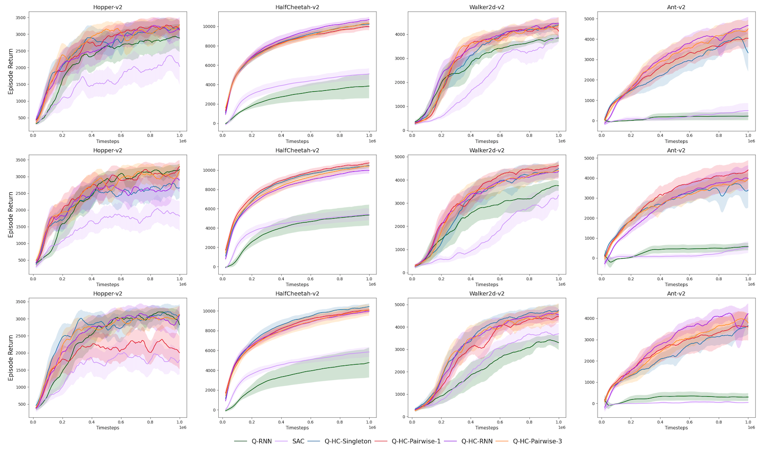
Figure 4: Comparisons of different implementations of ${\mathcal{Q}}$-HC with ${\mathcal{Q}}$-RNN and SAC. All tasks are sum-form PI-DRMDP tasks. The first line refers to the task with $n$ fixed as 20. The second line refers to the task with $n\sim U([15,20])$. The third line refers to the task with $n\sim U([10,20])$. All curves show the mean and one standard deviation of 6-7 seeds.

In Figure 5, we show the ablation study on the regulation term $L_{\text{reg}}$ on all 4 tasks. We observe that in HalfCheetah-v2 and Ant-v2, the regulation plays an important role for the final performance while the regulation is less necessary for the others. Besides, for ${\mathcal{Q}}$-HC algorithms with complex H-component architectures (i.e., ${\mathcal{Q}}$-HC-RNN, ${\mathcal{Q}}$-HC-Pairwise-3), the regulation is necessary while for simple structure like ${\mathcal{Q}}$-HC-Singleton, regulation is less helpful. We suspect that the simple structure itself imposes implicit regulation during the learning.

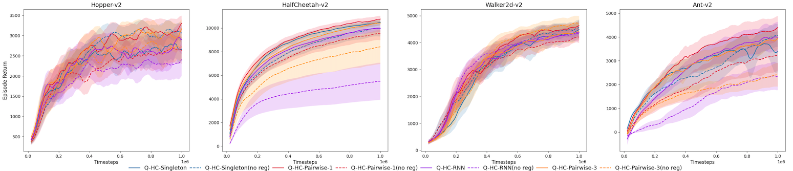
Figure 5: More ablations on $L_{\text{reg}}$ term. The task is a sum-form PI-DRMDP  with $n$ uniformly drawn from $15$ to $20$. Dashed lines are the no regularization version of the algorithm ${\mathcal{Q}}$-HC with the same color. All curves show the mean and a standard deviation of 6-7 seeds.

As mentioned in Section 4.1, we also analyze the HC-decomposition architecture on non sum-form PI-DRMDP taks based on OpenAI Gym. Two non sum-form tasks are included: Max and Square. For Max, $r(\tau_{t:t+n})=10\times\max_{i\in[t:t+n]}\{r(s_{i},a_{i})\}$ and $r(s_{i},a_{i})$ is the standard per-step reward in each task. For Square, we denote $r_{\text{avg}}(\tau_{t:t+n})=\frac{1}{n}\sum_{i\in[t:t+n]}r(s_{i},a_{i})$ and the reward is defined as follows. Noticing that these two tasks are still PI-DRMDP.

$$r(\tau_{t:t+n})=4\times\begin{cases}r_{\text{avg}}(\tau_{t:t+n})&|r_{\text{avg}}(\tau_{t:t+n})|<1.\\ \text{sign}(r_{\text{avg}}(\tau_{t:t+n}))\times r^{2}_{\text{avg}}(\tau_{t:t+n})&|r_{\text{avg}}(\tau_{t:t+n})|\geq 1.\end{cases}$$

The results are shown in Figure 6. Clearly, ${\mathcal{Q}}$-HC algorithms outperform ${\mathcal{Q}}$-RNN and vanilla SAC on all tasks. This suggests the benefit of HC-decomposition over other variants is remarkable.

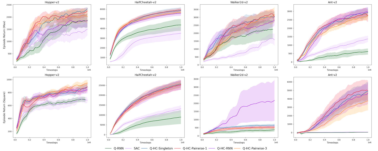
Figure 6: Experiments of non sum-form PI-DRMDP tasks. The first line shows the result of Max form and the second line shows the result of Square form. The learning curves are mean and one standard deviation of 6-7 seeds.

C.2 Comparative Evaluation

We show detailed results of our algorithms ${\mathcal{Q}}$-HC and previous baselines on sum-form PI-DRMDP  tasks with General Reward Function. Please refer to Appendix A and Appendix B for detailed discussions. For environments with maximal $c$ overlapping steps, the reward function is formally defined as follows.

$$r_{c}(\tau_{t_{i}-c:t_{i}+n_{i}})=\sum_{i\in[t_{i}-c:t_{i}+n_{i}-c]}r(s_{i},a_{i})$$

where $r(s_{i},a_{i})$ is the standard per-step reward. If $i<0$, then $r(s_{i},a_{i})=0$. In this definition, the reward is delayed by $c$ steps and thus the signal intervals are overlapped. In Figure 7, we show the relative average performance of each algorithm w.r.t the Oracle SAC trained on the dense reward setting. Please refer to Appendix D for the exact definition of this metric. The results demonstrate the superiority of our algorithms over the baselines in the General Reward Function experiments. This supports our claim that our algorithmic framework and the approximation method (HC) can be extended naturally to the general definition, i.e., PI-DRMDP-c.

Besides, we show the detailed learning curves of all algorithms in tasks with different overlapping steps $c$ in Figure 8.

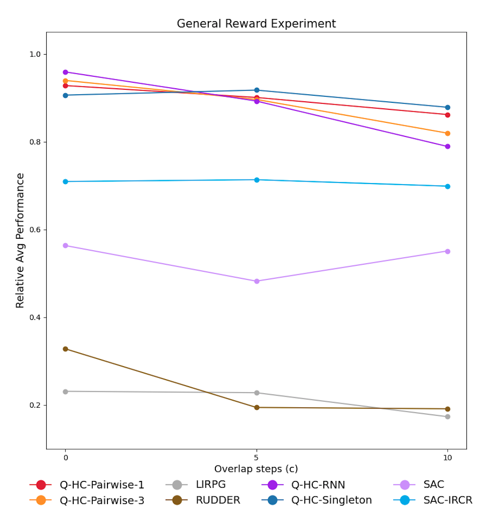
Figure 7: Relative Average Performance of our algorithms and the baselines on PI-DRMDP-c tasks with General Reward Functions. Each dot represents the relative performance of the algorithm over the PI-DRMDP-c task (average over Reach-v2, Hopper-v2, HalfCheetah-v2, Walker2d-v2, Ant-v2).

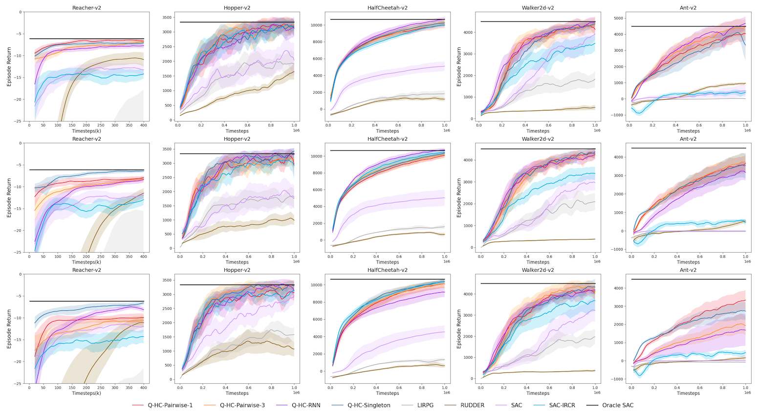
Figure 8: Learning curves of our algorithms $Q$-HC and several previous baselines. The first line refers to the task with $c=0$. The second line refers to the task with $c=5$. The third line refers to the task with $c=10$. All curves show the mean and one standard deviation of 6-7 seeds.

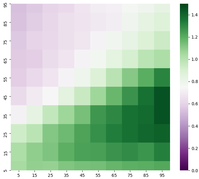
Figure 9: Visualization of $b_{\phi}(s_{t},a_{t})$ of ${\mathcal{Q}}$-HC-Singleton without regulation term.

Appendix D Experiment Details

D.1 Implementation Details of Our Algorithm

We re-implement SAC based on OpenAI baselines [32]. The corresponding hyperparameters are shown in Table 1. We use a smaller batch size due to limited computation power.

Table 1: Shared Hyperparameters with SAC

Hyperparameter	SAC
${\mathcal{Q}}_{\phi},\pi_{\theta}$ architecture	2 hidden-layer MLPs with 256 units each
non-linearity	ReLU
batch size	128
discount factor $\gamma$	0.99
optimizer	Adam [33]
learning rate	$3\times 10^{-4}$
entropy target	-$|A|$
target smoothing $\tau$	$0.005$
replay buffer	large enough for 1M samples
target update interval	1
gradient steps	1

To convince that the superiority of our algorithms (${\mathcal{Q}}$-HC-RNN, ${\mathcal{Q}}$-HC-Pairwise-K, ${\mathcal{Q}}$-HC-Singleton) results from the efficient approximation framework (Section 3.2) and the consistency with the theoretical analysis (Section 3.1), rather than from a better choice of hyper-parameters, we did not tune any hyper-parameter shared with SAC (i.e., in Table 1).

The architecture of different $H_{\phi}$s are shown as follows. For the regularization coefficient $\lambda$, we search $\lambda$ in $\{0.0,0.05,0.5,5.0\}$ for each implementation of ${\mathcal{Q}}$-HC. $\lambda$ is fixed for all tasks including the toy example.

1. ${\mathcal{Q}}$-HC-RNN. Each step’s input $\tau_{t:t+1}$ is first passed through a fully connected network with 48 hidden units and then fed into the GRU with a 48-unit hidden state. $H_{\phi}(\tau_{t_{i}:t})$ is the output of the GRU at the corresponding step. We use $\lambda=5.0$.

2. ${\mathcal{Q}}$-HC-Pairwise-1. Both $c^{0}_{\phi}$ and $c^{1}_{\phi}$ are two-layer MLPs with 64 hidden units each. $\lambda=0.5$.

3. ${\mathcal{Q}}$-HC-Pairwise-3. All $c^{i}_{\phi},i=0,1,2,3$ are two-layer MLP with 48 hidden units each. $\lambda=5.0$.

4. ${\mathcal{Q}}$-HC-Singleton. $b_{\phi}$ is a two-layer MLPs with 64 hidden units each. $\lambda=0.05$.

As suggested by the theoretical analysis, we augment the normalized $t-t_{i}$ to the state input.

All high dimensional experiments are based on OpenAI Gym [34] with MuJoCo200. All experiments are trained on GeForce GTX 1080 Ti and Intel(R) Xeon(R) CPU E5-2630 v4 @ 2.20GHz. Each single run can be completed within 36 hours.

D.2 Implementation Details of Other Baselines

${\mathcal{Q}}$-RNN. We use the same shared hyper-parameters as in Table 1. The only exception is the architecture of the GRU critic. Similar to ${\mathcal{Q}}$-HC-RNN, each state-action pair is first passed through a fully connected layer with 128 hidden units and ReLU activation. Then it is fed into the GRU network with 128-unit hidden state. The ${\mathcal{Q}}_{\phi}(\tau_{t_{i}:t+1})$ is the output of the GRU network at the corresponding step. We choose the above architecture to ensure that the number of parameters is roughly the same with our algorithm for fair comparison. The learning rate for the critic is still $3\times 10^{-4}$ after fine-tuning.

SAC-IRCR. Iterative Relative Credit Refinement [9] is implemented on episodic reward tasks. In the delayed reward setting, we replace the smoothing value (i.e., episode return) with the reward of the reward interval. We find this performs better than using the episode return.

D.3 Details for Toy Example

Point Reach. As illustrated in Figure 3(b), the Point Reach PI-DRMDP task consists of a 100x100 grid, the initial position at the bottom left corner, a 10x10 target area adjacent to the middle of the right edge and a point agent. The observation for the point agent is its $(x,y)$ coordinate only. The action space is its moving speed $(v_{x},v_{y})\in[-1,1]^{2}$ along the two directions. Since the agent can not observe the goal directly, it has to infer it from the reward signal. To relieve the agent from heavy exploration (not our focus), the delayed rewards provide some additional information to the agent as follows.

The grid is divided into 10 sub-areas of 10x100 along the x-axis. We denote the sub-areas (highlighted by one color each in Figure 3(a)) as $S_{i},i=[0:10]$ form left to right. In each sub-area $S_{i}$, it provides an extra reward and the reward $r^{i}$ indicates how far is the sub-area to the target (i.e., $r^{i}=i$). Clearly, the bigger the reward is, the closer the sub-area is to the target area. Besides, reward interval length is fixed as $20$ and the point agent is rewarded with the maximal $r^{i}$ it has visited in the interval together with a bonus after reaching the target and a punishment for not reaching. Namely,

$$r(\tau_{t:t+n})=\max_{j\in[t:t+n]}\sum_{i=0}^{9}r^{i}\cdot\bm{1}(s_{j:j+1}\in S_{i})+10\cdot(\bm{1}(\textit{reach target})-1)$$

The task ends once the agent reach the target area and also terminates after 500 steps. Clearly. the optimal policy is to go straightly from the initial point to the target area without hesitation. The shortest path takes roughly 95 steps. The learning curves in Figure 3(b) show the mean and half of a standard deviation of 10 seeds. All curves are smoothed equally for clarity.

Heatmap. In Figure 3(c), the heatmap visualizes the value of $b_{\phi}(s_{t},a_{t})$ on the whole grid. We select the $b_{\phi}$s after the training has converged to the optimal policy. To be specific of the visualization, for each of the 10x10 cells on the grid, $s_{t}$ in $b_{\phi}(s_{t},a_{t})$ is selected as the center of the cell and $a_{t}$ is sampled from $\pi(\cdot|s_{t},0)$. Additionally, in Figure 9, we visualize $b_{\phi}(s_{t},a_{t})$ similarly of ${\mathcal{Q}}$-HC-Singleton without $L_{\text{reg}}$. Clearly, Figure 9 shows the similar pattern as Figure 3(c).

D.4 Details for Variance Estimation

The experiment in Figure 1(c) is conducted in the following manner. First, we train a policy $\pi_{\theta}$ with ${\mathcal{Q}}$-HC-Singleton and collect all the samples along the training to the replay buffer $D$. Second, two additional critics are trained concurrently with samples uniformly sampled from $D$. One critic uses the GRU architecture (i.e., ${\mathcal{Q}}$-RNN) and the other uses ${\mathcal{Q}}$-HC-Singleton structure. Most importantly, since these two critics are not used for policy updates, there is no overestimation bias [14]. Thus, instead of using the CDQ method [14], these two critics are trained via the method in DDPG [22]. With a mini-batch from $D$, we compute the gradients on the policy’s parameters $\theta$ in Eq. (5) and Eq. (7) from the two extra critics respectively. Noticing that these gradients are not used in the policy training.

Then, we compute the sample variance of the gradient on each parameter $\theta_{i}$ in the policy network. The statistics (y-axis in Figure 1(c)) is the sum of variance over all parameters in the final layer (i.e., the layer that outputs the actions). The statistics is further averaged over the whole training and scaled uniformly for clarity.

D.5 Details for Relative Average Performance

Here, we formally introduce the Relative Average Performance (RAP) metric in Figure 2 and Figure 7. The relative average performance of algorithm $A$ on environment $C$ (with maximal overlapping steps $c$) is defined as the average of RAP over tasks in $\{\text{Reach-v2},\text{Hopper-v2},\text{HalfCheetah-v2},\text{Walker2d-v2},\text{Ant-v2}\}$. RAP of each task is the episodic return after 1M steps training normalized by the episodic return of Oracle SAC at 1M steps (trained on dense reward environment). The only exception is Reach-v2, in which the episodic returns are added by $50$ to before the normalization.

References

- Silver et al. [2017] David Silver, Julian Schrittwieser, Karen Simonyan, Aj Antonoglou, Ioannis abd Huang, Arthur Guez, Thomas Hubert, Lucas Baker, Matthew Lai, Adrian Bolton, Yutian Chen, Timothy Lillicrap, Fan Hui, Laurent Sifre, George van den Driessche, Thore Graepel, and Demis Hassabis. Mastering the game of go without human knowledge. Nature, 550, 2017.
- Mnih et al. [2015] Volodymyr Mnih, Koray Kavukcuoglu, David Silver, Andrei A Rusu, Joel Veness, Marc G Bellemare, Alex Graves, Martin Riedmiller, Andreas K Fidjeland, Georg Ostrovski, et al. Human-level control through deep reinforcement learning. Nature, 518(7540):529, 2015.
- Haarnoja et al. [2018a] Tuomas Haarnoja, Aurick Zhou, Kristian Hartikainen, George Tucker, Sehoon Ha, Jie Tan, Vikash Kumar, Henry Zhu, Abhishek Gupta, Pieter Abbeel, et al. Soft actor-critic algorithms and applications. arXiv preprint arXiv:1812.05905, 2018a.
- Hein et al. [2017] D. Hein, S. Depeweg, M. Tokic, S. Udluft, A. Hentschel, T. A. Runkler, and V. Sterzing. A benchmark environment motivated by industrial control problems. In 2017 IEEE Symposium Series on Computational Intelligence (SSCI), pages 1–8, 2017. doi: 10.1109/SSCI.2017.8280935.
- Gong et al. [2019] Yaobang Gong, Mohamed Abdel-Aty, Qing Cai, and Md Sharikur Rahman. Decentralized network level adaptive signal control by multi-agent deep reinforcement learning. Transportation Research Interdisciplinary Perspectives, 1:100020, 2019.
- Lin et al. [2018] Kaixiang Lin, Renyu Zhao, Zhe Xu, and Jiayu Zhou. Efficient large-scale fleet management via multi-agent deep reinforcement learning. In the 24th ACM SIGKDD International Conference, 2018.
- Olivecrona et al. [2017] Marcus Olivecrona, Thomas Blaschke, Ola Engkvist, and Hongming Chen. Molecular de-novo design through deep reinforcement learning. Journal of cheminformatics, 9(1):1–14, 2017.
- Xu et al. [2018] Zhe Xu, Zhixin Li, Qingwen Guan, Dingshui Zhang, and Jieping Ye. Large-scale order dispatch in on-demand ride-hailing platforms: A learning and planning approach. In the 24th ACM SIGKDD International Conference, 2018.
- Gangwani et al. [2020] Tanmay Gangwani, Yuan Zhou, and Jian Peng. Learning guidance rewards with trajectory-space smoothing. In 34th Conference on Neural Information Processing Systems, 2020.
- Zheng et al. [2018] Zeyu Zheng, Junhyuk Oh, and Satinder Singh. On learning intrinsic rewards for policy gradient methods. In Advances in Neural Information Processing Systems, volume 31, pages 4644–4654. Curran Associates, Inc., 2018.
- Oh et al. [2018] Junhyuk Oh, Yijie Guo, Satinder Singh, and Honglak Lee. Self-imitation learning. In Jennifer Dy and Andreas Krause, editors, Proceedings of the 35th International Conference on Machine Learning, volume 80 of Proceedings of Machine Learning Research, pages 3878–3887, Stockholmsmässan, Stockholm Sweden, 10–15 Jul 2018. PMLR.
- Klissarov and Precup [2020] Martin Klissarov and Doina Precup. Reward propagation using graph convolutional networks martin. In 34th Conference on Neural Information Processing Systems, 2020.
- Haarnoja et al. [2018b] Tuomas Haarnoja, Aurick Zhou, Pieter Abbeel, and Sergey Levine. Soft actor-critic: Off-policy maximum entropy deep reinforcement learning with a stochastic actor. In Proceedings of the 35th International Conference on Machine Learning, volume 80 of Proceedings of Machine Learning Research, pages 1861–1870, Stockholmsmässan, Stockholm Sweden, 10–15 Jul 2018b. PMLR.
- Fujimoto et al. [2018] Scott Fujimoto, Herke Hoof, and David Meger. Addressing function approximation error in actor-critic methods. In International Conference on Machine Learning, pages 1587–1596, 2018.
- Sutton and Barto [2018] Richard S Sutton and Andrew G Barto. Reinforcement learning: An introduction. MIT press, 2018.
- Cho et al. [2014] Kyunghyun Cho, Bart van Merriënboer, Caglar Gulcehre, Dzmitry Bahdanau, Fethi Bougares, Holger Schwenk, and Yoshua Bengio. Learning phrase representations using RNN encoder–decoder for statistical machine translation. In Proceedings of the 2014 Conference on Empirical Methods in Natural Language Processing (EMNLP), pages 1724–1734, Doha, Qatar, October 2014. Association for Computational Linguistics. doi: 10.3115/v1/D14-1179.
- Goodfellow et al. [2016] Ian Goodfellow, Yoshua Bengio, Aaron Courville, and Yoshua Bengio. Deep learning, volume 1. MIT Press, 2016.
- Arjona-Medina et al. [2019] Jose A. Arjona-Medina, Michael Gillhofer, Michael Widrich, Thomas Unterthiner, Johannes Brandstetter, and Sepp Hochreiter. Rudder: Return decomposition for delayed rewards. In Advances in Neural Information Processing Systems, volume 32, pages 13566–13577. Curran Associates, Inc., 2019.
- Schulman et al. [2017] John Schulman, Filip Wolski, Prafulla Dhariwal, Alec Radford, and Oleg Klimov. Proximal policy optimization algorithms. arXiv preprint arXiv:1707.06347, 2017.
- Duan et al. [2016] Yan Duan, Xi Chen, Rein Houthooft, John Schulman, and Pieter Abbeal. Benchmarking deep reinforcement learning for continuous control. In International Conference on Machine Learning, 2016.
- Degris et al. [2012] Thomas Degris, Martha White, and Richard S Sutton. Off-policy actor-critic. In Proceedings of the 29th International Coference on International Conference on Machine Learning, pages 179–186, 2012.
- Silver et al. [2014] David Silver, Guy Lever, Nicolas Heess, Thomas Degris, Daan Wierstra, and Martin Riedmiller. Deterministic policy gradient algorithms. In Proceedings of the 31st International Conference on International Conference on Machine Learning-Volume 32, pages I–387, 2014.
- Sutton [1984] Richard Stuart Sutton. Temporal credit assignment in reinforcement learning. PhD thesis, Department of Computer Science, University of Massachusetts at Amherst, 1984.
- Finn et al. [2020] Chelsea Finn, Pieter Abbeal, and Sergey Levine. Model-agnostic meta-learning for fast adaptation of deep networks. In 34th Conference on Neural Information Processing Systems, 2020.
- Gangwani et al. [2019] Tanmay Gangwani, Qiang Liu, and Jian Peng. Learning self-imitating diverse policies. In International Conference on Learning Representations, 2019.
- Guo et al. [2018] Yijie Guo, Junhyuk Oh, Satinder Singh, and Honglak Lee. Generative adversarial self-imitation learning. arXiv preprint arXiv:1812.00950, 2018.
- Liu et al. [2019] Yang Liu, Yunan Luo, Yuanyi Zhong, Xi Chen, Qiang Liu, and Jian Peng. Sequence modeling of temporal credit assignment for episodic reinforcement learning. arXiv preprint arXiv:1905.13420, 2019.
- Vaswani et al. [2017] Ashish Vaswani, Noam Shazeer, Niki Parmar, Jakob Uszkoreit, Llion Jones, Aidan Gomez, N, Lukasz Kaiser, and Illia Polosukhin. Attention is all you need. In 31th Conference on Neural Information Processing Systems, pages 5998–6008, 2017.
- Kipf and Welling [2016] Thomas N. Kipf and Max Welling. Semi-supervised classification with graph convolutional networks. CoRR, abs/1609.02907, 2016.
- Ng et al. [1999] A. Ng, D. Harada, and S. Russell. Policy invariance under reward transformations: Theory and application to reward shaping. In International Conference on Machine Learning, 1999.
- Levine et al. [2020] Sergey Levine, Aviral Kumar, George Tucker, and Justin Fu. Offline reinforcement learning: Tutorial, review, and perspectives on open problems. arXiv preprint arXiv:2005.01643, 2020.
- Dhariwal et al. [2017] Prafulla Dhariwal, Christopher Hesse, Oleg Klimov, Alex Nichol, Matthias Plappert, Alec Radford, John Schulman, Szymon Sidor, Yuhuai Wu, and Peter Zhokhov. Openai baselines. https://github.com/openai/baselines, 2017.
- Kingma and Ba [2014] Diederik Kingma and Jimmy Ba. Adam: A method for stochastic optimization. Computer Science, 2014.
- Greg et al. [2016] Brockman Greg, Cheung Vicki, Pettersson Ludwig, Schneider Jonas, Schulman John, Tang Jie, and Zaremba Wojciech. Openai gym, 2016.