A Clustering-based Framework for Classifying Data Streams

Abstract

The non-stationary nature of data streams strongly challenges traditional machine learning techniques. Although some solutions have been proposed to extend traditional machine learning techniques for handling data streams, these approaches either require an initial label set or rely on specialized design parameters. The overlap among classes and the labeling of data streams constitute other major challenges for classifying data streams. In this paper, we proposed a clustering-based data stream classification framework to handle non-stationary data streams without utilizing an initial label set. A density-based stream clustering procedure is used to capture novel concepts with a dynamic threshold and an effective active label querying strategy is introduced to continuously learn the new concepts from the data streams. The sub-cluster structure of each cluster is explored to handle the overlap among classes. Experimental results and quantitative comparison studies reveal that the proposed method provides statistically better or comparable performance than the existing methods.

1 Introduction

The recent advances in information technology have led to an increasing trend in the application of data streams, and data stream classification has captured the attention of many researchers. Unlike traditional classification problems, data streams are continuously evolving such that the data distributions can change dynamically and new data patterns may appear. This non-stationary nature of data streams, known as concept drift and concept evolution Masud et al. (2010); Gama et al. (2014), requires a continuous learning capability for traditional machine learning techniques to handle data streams Aggarwal et al. (2006); Bouchachia (2011); Mu et al. (2017). The scarcity of data labels and expensive labeling costs also limit the conventional classification techniques Din et al. (2020). Besides, limited time and memory space pose an additional layer of challenges for classifying the large volume of data streams.
To address these challenges, a great number of studies have been conducted on classifying data streams considering two primary aspects, data stream classification through: (i) supervised and (ii) semi-supervised learning. For supervised data stream classification frameworks, most studies Bifet et al. (2009); Bifet and Gavaldà (2009); Bifet et al. (2010b); Losing et al. (2018); Gomes et al. (2017) focus on extending traditional offline machine learning techniques with an assumption that the label of each incoming sample will be available after it is classified. However, this assumption does not always hold in real-world data stream classification problems and the labeling of data streams is time-consuming and expensive. Additionally, to adapt to the change in data streams, the optimization of the learnable parameters also imposes high computational overhead for supervised approaches.
Semi-supervised approaches Masud et al. (2012); Shao et al. (2016); Wagner et al. (2018); Zhu and Li (2020); Din et al. (2020) are developed as an alternative solution to perform data stream classifications using a small portion of labeled data and have shown substantial success. However, several challenges still remain. First, the detection of a novel class strongly depends on certain threshold parameters and the determination of threshold parameters is an open challenge. Secondly, the overlap among different classes is a common problem in data stream classification problems while very little research work has been conducted on handling data streams with overlapped classes. Thirdly, most of the existing semi-supervised classification frameworks classify data streams with partially labeled data in a passive learning manner. For better classification performance, this requires an effective labeling strategy to actively guide the learning procedure.
Considering the limitations of the existing methods described earlier, we propose a Clustering-based Data Stream Classification framework with Active Learning, namely CDSC-AL, to handle non-stationary data streams. The proposed framework consists of three main steps: (i) concept drift and novel class detection through clustering, (ii) novel concept learning and concept drift adaptation through active learning, and (iii) classification of data streams using label propagation. With these three steps, CDSC-AL aims to perform non-stationary data stream classification by reducing the labeling costs and handling the overlap among classes. In summary, the contributions of this paper are as follows:

• Extend a density-based data stream clustering method to capture concept drift and concept evolution for non-stationary data streams with a dynamic threshold.

• Develop an effective distance-based active learning procedure to query a small portion of labels for adapting to changes in data streams.

• Propose a classification procedure to handle the overlap among classes by investigating the sub-cluster structure inside clusters.

The remainder of this paper is organized as follows. Section 2 provides a review of the related work. The details of the CDSC-AL framework are discussed in Section 3 and the complexity analysis of the CDSC-AL framework is described in Section 4. Section 5 presents the experimental results and comparison studies with the state-of-the-art methods. Concluding remarks and future work are outlined in Section 6.

2 Related Work

Over the past few decades, great efforts have been conducted to adapt offline supervised learning techniques for classifying streaming data. In Aggarwal et al. (2006), the authors proposed a dynamic data classification framework using traditional classifiers to classify streaming data. A general framework was developed for adapting conventional classification techniques to perform data stream classification using clustering in Masud et al. (2010, 2012). In Bifet and Gavalda (2007); Bifet et al. (2013), ADaptive sliding WINdow (ADWIN) is proposed as a detector to capture the change of data streams and work collaboratively with traditional classification techniques for handling data streams. Later, ADWIN was widely used in ensemble-based data stream classification frameworks Bifet et al. (2010b); Gomes et al. (2017). To enhance the time and memory efficiency, a Self Adjusting Memory (SAM) model is introduced for offline classifiers to deal with non-stationary data streams in Losing et al. (2018).

Unlike supervised approaches, semi-supervised methods utilize a more realistic assumption on the availability of labels for data streams. The Linear Neighborhood Propagation Wang and Zhang (2007) method is used to perform data stream classification using a limited amount of labeled data. In Masud et al. (2012), ECSMiner is proposed to employ the clustering procedure for data stream classification in a semi-supervised manner. A combination of semi-supervised Support Vector Machines and k-means clustering is employed in Zhang et al. (2010) for classifying data streams. In Hosseini et al. (2016), data streams are divided into chunks and an ensemble of cluster-based classifiers is used to propagate labels among each chunk. The Co-forest algorithm Li and Zhou (2007) is extended for data stream classification using a small amount of labeled data in Wang and Li (2018).

Recently, online graph-based semi-supervised data stream classification frameworks were investigated in Ravi and Diao (2016); Wagner et al. (2018). In Ravi and Diao (2016), the authors continuously maintained a graph using both the labeled and unlabeled data over time and then predicted the label for incoming unlabeled instances through label propagation. Another novel online graph-based semi-supervised approach is introduced to reduce the time and memory complexity Wagner et al. (2018). Primarily, it utilizes a temporal label propagation procedure to not only label the new instances but also to learn from them.

Few recent studies on data stream classification incorporate active learning into the semi-supervised learning framework Lughofer et al. (2016); Mohamad et al. (2018). Such approaches handle the high labeling costs of data streams by actively querying labels for a small subset of interesting samples. In our proposed framework, we introduce a new active learning strategy to address the high labeling cost issue and combine it with a label propagation procedure to classify data streams in a semi-supervised manner.

3 Proposed Approach

In this section, the basic notations and assumptions for the CDSC-AL framework are introduced first. Then, we provide an overview of the CDSC-AL framework and discuss its three main components: concept drift and evolution detection through clustering, the adaptation of drifted and novel concepts using active learning, and classification through label propagation.

3.1 Notations and Assumptions

Notations.

Let $DS$ be an unknown data stream and $CH_{t}$ is a chunk of data from $DS$ such that $DS=\bigcup^{\infty}_{t=1}\{CH_{t}\}$ where $t$ refers to the time index of a data chunk. For each data chunk, $CH_{t}=\bigcup^{|CH_{t}|}_{i=1}\{\mathbf{x^{i}_{t}}|\mathbf{x^{i}_{t}}\in\mathcal{R}^{m}\}$ where $\mathbf{x^{i}_{t}}$ denotes a data sample in $CH_{t}$ and $m$ is the dimension of $\mathbf{x^{i}_{t}}$. Assume $HS_{t}=\{GS_{t},LS_{t}\}$ is the summary of a data stream where $GS_{t}$ and $LS_{t}$ represent the macro-level and the micro-level summary of $DS$. We use $Z^{i}_{t}$ to represent the $i^{th}$ cluster center of $DS$ at time $t$, and $SC^{i,j}_{t}$ refers to the $j^{th}$ sub-cluster center of cluster $i$ at time $t$. The notation $y^{i,j}_{t}$ denotes the class label of $SC^{i,j}_{t}$.

Assumptions.

Considering the non-stationary nature of data streams, the proposed CDSC-AL framework assumes:

• The characteristics of data streams can change abruptly or gradually.

• Multiple novel concepts may arise simultaneously.

• Overlapped classes will appear over time.

3.2 An Overview of CDSC-AL Framework

A general algorithm description of the CDSC-AL framework is presented in Algorithm 1. We extended the recently developed density-based stream clustering algorithm, namely dynamic fitness proportionate sharing (DFPS-clustering) Yan et al. (2019, 2020), to perform the classification of data streams considering several aspects. First, a new merge procedure between clusters from the incoming data chunk and historical clusters is employed and the modified merge procedure is used to detect novel classes and drifted classes. Second, two levels of cluster summary are maintained continuously to reflect the characteristics of the data stream through an active learning procedure. Third, an effective classification procedure using the k-nearest-neighbor (KNN) rule Altman (1992) is introduced to classify the incoming data chunk based on the summary and queried labels. Additionally, the overlap among classes is addressed by exploring the sub-cluster information from the micro-level summary.

Algorithm 1 An overview of CDSC-AL framework

Input: $DS$
Parameters: $C_{t}$: the set of clusters at time $t$; $CH_{t}$: the current data chunk; $C_{CH_{t}}$: a set of clusters discovered in $CH_{t}$; $Q_{t}$: a small set of samples for active label querying in $CH_{t}$; $Y_{Q_{t}}$: the label set of the queried samples $Q_{t}$; $Y_{CH_{t}}$: the label set for $CH_{t}$.
Output: $HS_{t}$

1:for $t=1$ to $\infty$ do

2:    Conduct recursive density evaluation on $CH_{t}$ and rank all samples of $CH_{t}$ according to their density values

3:    Perform the search of possible clusters in $CH_{t}$

4:    Merge highly overlapped clusters to obtain $C_{CH_{t}}$

5:    if $t==1$ then

6:        $HS_{t}=\emptyset$, $C_{t}=C_{CH_{t}}$

7:        $\left[Q_{t},Y_{Q_{t}}\right]$ = ActiveQuery$(HS_{t},C_{t},CH_{t})$

8:        $Y_{CH_{t}}$=Classify$(HS_{t},Q_{t},Y_{Q_{t}},CH_{t})$

9:        $HS_{t}$=ClusteringModel$(HS_{t},C_{CH_{t}},CH_{t})$

10:    else

11:        $C_{t}$=CheckMerge$(HS_{t},C_{CH_{t}},CH_{t})$

12:        $\left[Q_{t},Y_{Q_{t}}\right]$=ActiveQuery$(HS_{t},C_{t},CH_{t})$

13:        $Y_{CH_{t}}$=Classify$(HS_{t},Q_{t},Y_{Q_{t}},CH_{t})$

14:        $HS_{t}$=ClusteringModel$(HS_{t},C_{CH_{t}},CH_{t})$

15:    end if

16:    Return $HS_{t}$

17:end for

3.3 Concept Drifts and Evolution Detection through Clustering

To capture the non-stationary property of data streams, we modified the DFPS-clustering algorithm substantially by employing a new cluster merge procedure between the historical clusters and new clusters. Then, we use the new DFPS-clustering method to distinguish novel concepts from drifted concepts. Algorithm 2 summarizes the new cluster merge procedure for the detection of drifted and novel concepts.
As shown in Algorithm 2, the new merge procedure utilizes the density of boundary instances to decide whether a merge should happen between a historical cluster and its neighboring cluster from $CH_{t}$. Then, it generates two types of clusters: (i) novel clusters and (ii) updated clusters. Clusters that are not merged with historical clusters are considered as novel clusters while the merged clusters are defined as updated clusters. Based on these two types of clusters, the novel concepts are captured by novel clusters and drifted concepts are identified as updated clusters. To validate the existence of novel clusters, we use the mean and standard deviation of the density values of historical clusters to compute a dynamic density threshold. Let $C^{no}_{t}$ be a novel cluster and $F_{C^{no}_{t}}$ be its density value. The mean and standard deviations of historical clusters are denoted as $\mu(F_{C_{t}})$ and $\sigma(F_{C_{t}})$, respectively. The following Remark is defined for novel cluster detection.

Remark 1.

If $F_{C^{no}_{t}}\geq|\mu(F_{C_{t}})-\sigma(F_{C_{t}})|$, then $C^{no}_{t}$ is a true novel cluster.

Remark 1 is derived from the three-sigma principle of Gaussian distribution used in Yan et al. (2019) and it means a cluster is considered as a valid novel cluster if its density value falls inside the one-sigma distance from the average density of historical clusters at time $t$. With Remark 1, a novel cluster detector with a dynamic density threshold is used for validating the existence of novel clusters.

Algorithm 2 New cluster merge procedure

Parameters: $L_{NC}$: a list of paired clusters between a historical cluster and its neighboring clusters in $CH_{t}$, $X_{B}$: a set of boundary samples between each pair of clusters in $L_{NC}$

1:procedure CheckMerge($HS_{t}$, $C_{CH_{t}}$, $CH_{t}$)

2:    Identify the paired neighboring historical clusters in $HS_{t}$ for $C_{CH_{t}}$ to obtain $L_{NC}$

3:    Extract $X_{B}$ for each pair of neighboring clusters in $L_{NC}$

4:    Evaluate the density of $X_{B}$ and check for the density drop for each pair of neighboring clusters

5:    Merge each pair of neighboring clusters when there is no density drop in $X_{B}$

6:    Mark unmerged clusters as novel clusters and merged clusters as updated clusters

7:    Validate the existence of novel clusters using Remark 1

8:    Return $C_{t}=\left[novel\text{ }clusters,updated\text{ }clusters\right]$

9:end procedure

3.4 Adaptation of Drifted and Novel Concepts using Active Learning

Considering time and space constraints, we maintain a summary of the data stream rather than keeping all historical samples from $DS$. The maintained summary $HS_{t}$ consists of two levels of summary on $DS$: (i). macro-level summary $GS_{t}$, and (ii) micro-level summary $LS_{t}$. The definitions of these two levels of summary are expressed as:

$$GS_{t}=\bigcup^{|C_{t}|}_{i=1}[Z^{i}_{t},F^{i}_{t},R^{i}_{t}],$$ (1)

and

$$LS_{t}=\bigcup^{|C_{t}|}_{i=1}\{\bigcup^{|SC^{i}_{t}|}_{j=1}[SC^{i,j}_{t},y^{i,j}_{t}]\}.$$ (2)

Where $F^{i}_{t}$ and $R^{i}_{t}$ denote the density value and radius of the $i^{th}$ cluster at time $t$, respectively. $y^{i,j}_{t}$ refers to the class label of $SC^{i,j}_{t}$ and all samples from $SC^{i,j}_{t}$ share the same label. $LS_{t}$ is used to explore the sub-cluster structure of each cluster when classes are highly overlapped. Specifically, we split each cluster into a set of sub-clusters such that each sub-cluster only has a unique class label. Instead of computing the mean vector for each sub-cluster, we consider only the sample with the highest density value in each sub-cluster as the sub-cluster center and use it for label propagation.

These two levels of summary are continuously updated to adapt to the change of $DS$ using an active learning procedure. Since two types of clusters can be obtained from the clustering analysis, a hybrid active learning strategy of informative-based and representative-based sampling is introduced to reduce the labeling costs. The adaptation procedure of these two levels of summary is provided in Algorithm 3. In Algorithm 3, for novel clusters, the representative-based query Gu et al. (2019) is performed by sampling from the centers of clusters. On the other hand, we conduct the informative-based query Gu et al. (2019) in updated clusters through a distance-based strategy. Unlike the entropy-based sampling Lughofer et al. (2016) strategy, samples that are relatively far from the updated clusters are selected as informative samples for label querying. Let $Q_{t}$ be the set of queried samples and $Y_{Q_{t}}$ be the label set for $Q_{t}$. After the active label query, the label propagation procedure begins to predict the label of the remaining samples in $CH_{t}$ using $Y_{Q_{t}}$ and $HS_{t}$. Finally, the predicted labels are used to update the $LS_{t}$ with a two-step procedure. First, we update the centers of sub-clusters within updated clusters with new samples that have higher density values. Second, we create a set of new sub-clusters for each novel cluster to capture the characteristics of novel concepts.

Algorithm 3 Adaptation of drifted and novel concepts

Parameters: $X_{no}$: a set of samples from novel clusters; $X_{up}$: a set of samples from updated clusters; $Q_{I}$: a set of queried samples using the Informative-based sampling; $Q_{R}$: a set of queried samples using Representative-based sampling; $Y_{CH_{t}}$: the label set for $CH_{t}$.

1:procedure ClusteringModel($HS_{t}$, $C_{t}$, $CH_{t}$)

2:    $\left[Q_{t},Y_{Q_{t}}\right]$=ActiveQuery($C_{t}$, $CH_{t}$)

3:    $Y_{CH_{t}}$=Classify$(HS_{t},Q_{t},Y_{Q_{t}},CH_{t})$

4:    Update the $GS_{t}$ according to $C_{t}$

5:    Update the $LS_{t}$ using $Y_{CH_{t}}$

6:    return $HS_{t}=[GS_{t},LS_{t}]$

7:end procedure

8:procedure ActiveQuery($C_{t},CH_{t}$)

9:    Extract novel clusters and updated clusters from $C_{t}$

10:    Identify samples that are close to the novel clusters as $X_{no}$

11:    Identify samples that are close to updated clusters as $X_{up}$

12:    Representative-based sampling for $X_{no}$ to obtain $Q_{R}$

13:    Informative-based sampling for $X_{up}$ to obtain $Q_{I}$

14:    $Q_{t}=(Q_{I}\cup Q_{R})$

15:    Query labels from human experts to obtain $Y_{Q_{t}}$

16:    return $\left[Q_{t},Y_{Q_{t}}\right]$

17:end procedure

3.5 Classification through Label Propagation

To classify an incoming data chunk, we employ an effective label propagation procedure based on $HS_{t}$ and $Q_{t}$. First, a set of prototypes with label information are obtained from $HS_{t}$ and $Q_{t}$. Then, the KNN-based classification procedure is employed to propagate the labels of the prototypes to samples in $CH_{t}$. Here, we set the value of $k$ to five and the classification procedure is presented in Algorithm 4.

4 Complexity Analysis

Here, we discussed the time and memory complexity of the CDSC-AL framework using the following parameters:

• $n$: the number of samples from an incoming data chunk

• $m$: the number of dimensions of an incoming instance

• $|SC_{t}|$: the total number of sub-clusters at time $t$

• $|C_{t}|$: the total number of clusters at time $t$

• $k$: the number of nearest neighbors

• $|Q_{t}|$ the number of queried samples at time $t$

Algorithm 4 Classification through label propagation

Parameters: $Y_{CH_{t}}$: the label set for $CH_{t}$; $Sub_{r}$: a set of representatives from sub-clusters; $P_{t}$: a set of prototypes with labels.

1:procedure Classify($HS_{t},Q_{t},Y_{Q_{t}},CH_{t}$)

2:    Extract sub-cluster centers and its labels from $HS_{t}$ as $Sub_{r}$

3:    $P_{t}=Sub_{r}\cup[Q_{t},Y_{Q_{t}}]$

4:    Propagate labels from the prototype set to samples in $CH_{t}$ using KNN rule and obtain the predicted label set $Y_{CH_{t}}$

5:    return $Y_{CH_{t}}$

6:end procedure

Time Complexity.

The density evaluation of the new DFPS-clustering procedure requires $O(n^{2}m)$ distance calculations. To update $HS_{t}$, there will be $O(nm|C_{t}|+nm|SC_{t}|)\leq O(2nm|SC_{t}|)$ distance calculations where $|C_{t}|\leq|SC_{t}|$. The classification of the incoming data chunk will require $O(knm(|SC_{t}|+|Q_{t}|))$ distance calculations. Thus, the total time complexity of a single data chunk in terms of distance calculations is expressed as: $O(n^{2}m+2nm|SC_{t}|+knm(|SC_{t}|+|Q_{t}|))$.

Memory Complexity.

For $LS_{t}$, the memory space complexity is expressed as $O(|SC_{t}|(m+1))\approx O(m|SC_{t}|)$. In terms of $GS_{t}$, it takes $O(|C_{t}|(m+2))\approx O(m|C_{t}|)$ memory space. The total memory complexity will be $O(m(|SC_{t}|+|C_{t}|))$.

5 Experimental Studies and Discussions

In this section, experiments are conducted on the CDSC-AL framework using nine benchmark datasets, and comparison studies with the state-of-the-art methods are presented.

5.1 Experimental Setup

Datasets	Sample	Dimensions	Classes	Overlap
Syn-1	18900	2	9	False
Syn-2	11400	2	10	True
Sea	60000	2	3	False
KDD99	494021	34	5	False
Forest	581012	11	7	True
GasSensor	13910	128	6	True
Shuttle	58000	9	7	False
MNIST	70000	784	10	False
CIFAR10	60000	3072	10	False

Table 1: Dataset descriptions.

Datasets and Streaming Settings.

Nine multi-class benchmark datasets, including three synthetic datasets and six well-known real datasets from Dheeru and Karra Taniskidou (2017), are used in the experiments for performance evaluation. Table 1 summarizes these datasets in terms of sample size, dimensionality, number of classes, and class overlap. According to Table 1, the Forest, Syn-2, CIFAR10, and GasSensor datasets have highly overlapped classes. Following the setting in Aggarwal et al. (2006); Din et al. (2020), we partition each benchmark dataset into a number of data chunks with a fixed size of $1000$ samples and pass them sequentially to each algorithm in the experiment. In Syn-1, Syn-2, Sea, and Shuttle datasets, data chunks are arranged in an order to simulate abrupt concept drifts. For remaining datasets, we arrange data chunks in an order that generates the gradual concept drifts.

Dataset	Metric	LNP	OReSSL	CDSC-AL
Syn-1	BA	$0.8869(3)$	$0.9307(2)$	$\mathbf{0.9459(1)}$
	$F_{mac}$	$0.7939(3)$	$0.9318(2)$	$\mathbf{0.9490(1)}$
Syn-2	BA	$0.8338(3)$	$\mathbf{0.8481(1)}$	$0.8459(2)$
	$F_{mac}$	$0.6375(3)$	$0.7899(2)$	$\mathbf{0.8149(1)}$
Sea	BA	$0.5262(3)$	$0.8206(2)$	$\mathbf{0.9691(1)}$
	$F_{mac}$	$0.6019(3)$	$0.8275(2)$	$\mathbf{0.9729(1)}$
KDD99	BA	$0.5362(3)$	$0.6831(2)$	$\mathbf{0.8364(1)}$
	$F_{mac}$	$0.5311(3)$	$0.7076(2)$	$\mathbf{0.7921(1)}$
Forest	BA	$0.5181(3)$	$0.7153(2)$	$\mathbf{0.8465(1)}$
	$F_{mac}$	$0.5258(3)$	$0.7114(2)$	$\mathbf{0.8230(1)}$
GasSensor	BA	$0.6479(3)$	$0.8841(2)$	$\mathbf{0.8916(1)}$
	$F_{mac}$	$0.6611(3)$	$0.8674(2)$	$\mathbf{0.8995(1)}$
Shuttle	BA	$0.4172(3)$	$0.4709(2)$	$\mathbf{0.4744(1)}$
	$F_{mac}$	$0.4119(3)$	$\mathbf{0.4862(1)}$	$0.4789(2)$
MNIST	BA	$0.7682(3)$	$0.8806(2)$	$\mathbf{0.9669(1)}$
	$F_{mac}$	$0.7725(3)$	$0.8828(2)$	$\mathbf{0.9676(1)}$
CIFAR10	BA	$0.4158(3)$	$0.6421(2)$	$\mathbf{0.7857(1)}$
	$F_{mac}$	$0.4195(3)$	$0.6344(2)$	$\mathbf{0.7869(1)}$
Avg. ranks	BA	$3.00$	$1.78$	$\mathbf{1.22}$
	$F_{mac}$	$3.00$	$1.89$	$\mathbf{1.11}$

Table 2: Performance comparison with semi-supervised methods. (Relative rank of each algorithm is shown within parentheses.)

Compared Methods.

We compared the CDSC-AL framework with the state-of-the-art methods considering two aspects: (i) comparison with semi-supervised approaches, and (ii) comparison with supervised approaches. We selected two existing semi-supervised methods, namely OReSSL Din et al. (2020) and LNP Wang and Zhang (2007), and results are summarized in Table 2. Four supervised methods, including Leverage Bagging (LB) Bifet et al. (2010b), OZA Bag ADWIN (OBA) Bifet et al. (2009), Adaptive Hoeffding Tree (AHT) Bifet and Gavaldà (2009), and SAMkNN Losing et al. (2018), are used for the second comparison study. The results are presented in Table 3. The MATLAB code for semi-supervised methods is released by the authors and all codes for supervised methods can be found on the Massive Online Analysis (MOA) framework Bifet et al. (2010a). The python code of the CDSC-AL framework is available at the link. All experiments are conducted on an Intel Xeon (R) machine with 64GB RAM operating on Microsoft Windows 10.

Parameter Setting.

For the semi-supervised methods and CDSC-AL, the portion of labeled data of each incoming data chunk is set as $10\%$. For supervised methods, the labels of all samples from an incoming data chunk are provided to update the classifier after classification while CDSC-AL utilized only $10\%$ labeled data.

Evaluation Metrics.

Due to the imbalanced class distributions in benchmark datasets, we use the balanced classification accuracy ($BA$) Brodersen et al. (2010) and the macro-average of F-score ($F_{mac}$) Kelleher et al. (2020) as performance evaluation metrics. We recorded these two metrics over the entire data stream classification and reported the average values for performance evaluation. The best results are highlighted in bold-face. The Friedman and Nemenyi post-hoc tests Demšar (2006) are employed to statistically analyze the experimental results with a significance level of $0.05$.

Dataset	Metric	LB	OBA	AHT	SAMkNN	CDSC-AL
Syn-1	BA	$0.7910(2)$	$0.6640(3)$	$0.6354(4)$	$0.6247(5)$	$\mathbf{0.9459(1)}$
	$F_{mac}$	$0.7965(2)$	$0.6675(3)$	$0.6513(4)$	$0.6313(5)$	$\mathbf{0.9490(1)}$
Syn-2	BA	$0.7124(2)$	$0.7204(3)$	$0.6926(4)$	$0.6784(5)$	$\mathbf{0.8459(1)}$
	$F_{mac}$	$0.7218(2)$	$0.7219(3)$	$0.6977(4)$	$0.6864(5)$	$\mathbf{0.8149(1)}$
Sea	BA	$0.8204(2)$	$0.7498(3)$	$0.7493(4)$	$0.7205(5)$	$\mathbf{0.9691(1)}$
	$F_{mac}$	$0.8227(2)$	$0.7501(4)$	$0.7505(3)$	$0.7345(5)$	$\mathbf{0.9729(1)}$
KDD99	BA	$0.7585(4)$	$0.7812(3)$	$\mathbf{0.8541(1)}$	$0.7495(5)$	$0.8364(2)$
	$F_{mac}$	$0.7564(4)$	$0.7798(3)$	$\mathbf{0.8012(1)}$	$0.7682(5)$	$0.7921(2)$
Forest	BA	$\mathbf{0.8888(1)}$	$0.8707(2)$	$0.8612(3)$	$0.8545(4)$	$0.8465(5)$
	$F_{mac}$	$\mathbf{0.8901(1)}$	$0.8709(2)$	$0.8688(3)$	$0.8588(4)$	$0.8230(5)$
GasSensor	BA	$0.7185(2)$	$0.6345(4)$	$0.6111(3)$	$0.6357(5)$	$\mathbf{0.8916(1)}$
	$F_{mac}$	$0.7199(2)$	$0.6361(4)$	$0.6188(3)$	$0.6412(5)$	$\mathbf{0.8995(1)}$
Shuttle	BA	$\mathbf{0.4789(1)}$	$0.4477(4)$	$0.4508(3)$	$0.4424(5)$	$0.4744(2)$
	$F_{mac}$	$\mathbf{0.5187(1)}$	$0.5112(2)$	$0.4978(3)$	$0.4894(4)$	$0.4789(5)$
MNIST	BA	$0.8909(2)$	$0.8498(4)$	$0.8393(5)$	$0.8549(3)$	$\mathbf{0.9669(1)}$
	$F_{mac}$	$0.8946(2)$	$0.8501(4)$	$0.8412(5)$	$0.8596(3)$	$\mathbf{0.9676(1)}$
CIFAR10	BA	$0.7199(3)$	$0.6208(5)$	$0.7366(2)$	$0.6218(4)$	$\mathbf{0.7857(1)}$
	$F_{mac}$	$0.7208(2)$	$0.6325(4)$	$0.7381(3)$	$0.6295(5)$	$\mathbf{0.7869(1)}$
Avg. ranks	BA	$2.00$	$2.86$	$3.57$	$4.57$	$\mathbf{1.86}$
	$F_{mac}$	$1.75$	$2.63$	$3.00$	$4.00$	$\mathbf{2.00}$

Table 3: Performance comparison with supervised methods. (Relative rank of each algorithm is shown within parentheses.)

5.2 Results and Discussions

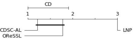
Figure 1: Comparison of CDSC-AL against semi-supervised methods with the Nemenyi test with $\alpha=0.05$ using $BA$.

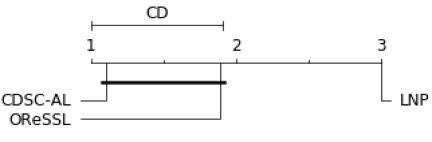
Figure 2: Comparison of CDSC-AL against semi-supervised methods with the Nemenyi test with $\alpha=0.05$ using $F_{mac}$.

Comparison with Semi-supervised Methods.

To compare the CDSC-AL method with the OReSSL and LNP methods, we repeated each experiment ten times and the average results are presented in Table 2. From Table 2, the balanced classification accuracy shows that the CDSC-AL method outperforms the other two methods on most data streams with the lowest rank of $1.11$. In terms of $F_{mac}$, CDSC-AL also provides better performance on most data streams. For data streams with abrupt concept drifts, CDSC-AL still achieves slightly better or comparable performance. From the Nemenyi post-hoc test, Figures 1 and 2 reveal that there is a statistically significant difference between CDSC-AL and LNP in terms of $BA$ and $F_{mac}$. Although CDSC-AL shows statistically comparable performance with the OReSSL method, it does not require any parameter optimization or an initial set of labeled data.

Comparison with Supervised Methods.

Table 3 presents the results of CDSC-AL and the four supervised methods. Using only $10\%$ of the labels, Table 3 demonstrates that the CDCS-AL method achieves the best performance on six of the benchmark data streams including Syn-1, Syn-2, Sea, GasSensor, MNIST, and CIFAR10. In Figures 3 and 4, CDCS-AL shows statistically comparable performance to the LB, OBA, and AHT methods on the remaining three data streams from the Nemenyi test. Also, CDSC-AL has statistically better performance than the SAMkNN approach. For data streams with abrupt concept drifts, CDSC-AL presents slightly better or comparable performance relative to supervised approaches. In summary, the comparison study with supervised methods reveals that CDSDF-AL always provides statistically better or comparable performance than the supervised methods using only a small proportion of labeled data.

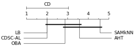
Figure 3: Comparison of CDSC-AL against supervised methods with the Nemenyi test with $\alpha=0.05$ using $BA$.

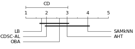
Figure 4: Comparison of CDSC-AL against supervised methods with the Nemenyi test with $\alpha=0.05$ using $F_{mac}$.

6 Conclusions and Future Work

We presented a clustering-based data stream classification framework through active learning (CDSC-AL) to handle non-stationary data streams. We developed a new cluster merge procedure as a part of the new DFPS-clustering procedure and used the new DFPS-clustering procedure to capture the drifted concepts and novel concepts. Two levels of cluster summaries were maintained to effectively classify the incoming data samples in the presence of overlapped classes, and an active learning technique was introduced to learn the change of data distributions. The primary advantages of the CDSC-AL method can be summarized from several points of view: (i) no dependency on initial label set, (ii) effective detection for drifted concepts and novel concepts with dynamic threshold, and (iii) high-quality classification performance in the presence of overlapped classes with a small proportion of labeled data. The comparison studies with the semi-supervised and supervised methods justify the efficacy of CDSC-AL methods on both synthetic and real data.
In the future, we will investigate solutions to reduce the time complexity of CDSC-AL and implement the CDSC-AL framework in some real-world applications such as text/image stream classifications.

References

- Aggarwal et al. [2006] Charu C Aggarwal, Jiawei Han, Jianyong Wang, and Philip S Yu. A framework for on-demand classification of evolving data streams. IEEE Transactions on Knowledge and Data Engineering, 18(5):577–589, 2006.
- Altman [1992] Naomi S Altman. An introduction to kernel and nearest-neighbor nonparametric regression. The American Statistician, 46(3):175–185, 1992.
- Bifet and Gavalda [2007] Albert Bifet and Ricard Gavalda. Learning from time-changing data with adaptive windowing. In Proceedings of the 2007 SIAM international conference on data mining, pages 443–448. SIAM, 2007.
- Bifet and Gavaldà [2009] Albert Bifet and Ricard Gavaldà. Adaptive learning from evolving data streams. In International Symposium on Intelligent Data Analysis, pages 249–260. Springer, 2009.
- Bifet et al. [2009] Albert Bifet, Geoff Holmes, Bernhard Pfahringer, Richard Kirkby, and Ricard Gavaldà. New ensemble methods for evolving data streams. In Proceedings of the 15th ACM SIGKDD international conference on Knowledge discovery and data mining, pages 139–148, 2009.
- Bifet et al. [2010a] Albert Bifet, Geoff Holmes, Richard Kirkby, and Bernhard Pfahringer. MOA: massive online analysis. J. Mach. Learn. Res., 11:1601–1604, 2010.
- Bifet et al. [2010b] Albert Bifet, Geoff Holmes, and Bernhard Pfahringer. Leveraging bagging for evolving data streams. In Joint European conference on machine learning and knowledge discovery in databases, pages 135–150. Springer, 2010.
- Bifet et al. [2013] Albert Bifet, Bernhard Pfahringer, Jesse Read, and Geoff Holmes. Efficient data stream classification via probabilistic adaptive windows. In Proceedings of the 28th annual ACM symposium on applied computing, pages 801–806, 2013.
- Bouchachia [2011] Abdelhamid Bouchachia. Incremental learning with multi-level adaptation. Neurocomputing, 74(11):1785–1799, 2011.
- Brodersen et al. [2010] Kay Henning Brodersen, Cheng Soon Ong, Klaas Enno Stephan, and Joachim M Buhmann. The balanced accuracy and its posterior distribution. In 2010 20th International Conference on Pattern Recognition, pages 3121–3124. IEEE, 2010.
- Demšar [2006] Janez Demšar. Statistical comparisons of classifiers over multiple data sets. Journal of Machine learning research, 7(Jan):1–30, 2006.
- Dheeru and Karra Taniskidou [2017] Dua Dheeru and Efi Karra Taniskidou. UCI machine learning repository, 2017.
- Din et al. [2020] Salah Ud Din, Junming Shao, Jay Kumar, Waqar Ali, Jiaming Liu, and Yu Ye. Online reliable semi-supervised learning on evolving data streams. Information Sciences, 2020.
- Gama et al. [2014] João Gama, Indrė Žliobaitė, Albert Bifet, Mykola Pechenizkiy, and Abdelhamid Bouchachia. A survey on concept drift adaptation. ACM computing surveys (CSUR), 46(4):1–37, 2014.
- Gomes et al. [2017] Heitor Murilo Gomes, Jean Paul Barddal, Fabrício Enembreck, and Albert Bifet. A survey on ensemble learning for data stream classification. ACM Computing Surveys (CSUR), 50(2):1–36, 2017.
- Gu et al. [2019] Shilin Gu, Yang Cai, Jincheng Shan, and Chenping Hou. Active learning with error-correcting output codes. Neurocomputing, 364:182–191, 2019.
- Hosseini et al. [2016] Mohammad Javad Hosseini, Ameneh Gholipour, and Hamid Beigy. An ensemble of cluster-based classifiers for semi-supervised classification of non-stationary data streams. Knowledge and information systems, 46(3):567–597, 2016.
- Kelleher et al. [2020] John D Kelleher, Brian Mac Namee, and Aoife D’arcy. Fundamentals of machine learning for predictive data analytics: algorithms, worked examples, and case studies. MIT press, 2020.
- Li and Zhou [2007] Ming Li and Zhi-Hua Zhou. Improve computer-aided diagnosis with machine learning techniques using undiagnosed samples. IEEE Transactions on Systems, Man, and Cybernetics-Part A: Systems and Humans, 37(6):1088–1098, 2007.
- Losing et al. [2018] Viktor Losing, Barbara Hammer, and Heiko Wersing. Tackling heterogeneous concept drift with the self-adjusting memory (sam). Knowledge and Information Systems, 54(1):171–201, 2018.
- Lughofer et al. [2016] Edwin Lughofer, Eva Weigl, Wolfgang Heidl, Christian Eitzinger, and Thomas Radauer. Recognizing input space and target concept drifts in data streams with scarcely labeled and unlabelled instances. Information Sciences, 355:127–151, 2016.
- Masud et al. [2010] Mohammad Masud, Jing Gao, Latifur Khan, Jiawei Han, and Bhavani M Thuraisingham. Classification and novel class detection in concept-drifting data streams under time constraints. IEEE Transactions on Knowledge and Data Engineering, 23(6):859–874, 2010.
- Masud et al. [2012] Mohammad M Masud, Clay Woolam, Jing Gao, Latifur Khan, Jiawei Han, Kevin W Hamlen, and Nikunj C Oza. Facing the reality of data stream classification: coping with scarcity of labeled data. Knowledge and information systems, 33(1):213–244, 2012.
- Mohamad et al. [2018] Saad Mohamad, Moamar Sayed-Mouchaweh, and Abdelhamid Bouchachia. Active learning for classifying data streams with unknown number of classes. Neural Networks, 98:1–15, 2018.
- Mu et al. [2017] Xin Mu, Feida Zhu, Juan Du, Ee-Peng Lim, and Zhi-Hua Zhou. Streaming classification with emerging new class by class matrix sketching. In Proceedings of the AAAI Conference on Artificial Intelligence, volume 31, 2017.
- Ravi and Diao [2016] Sujith Ravi and Qiming Diao. Large scale distributed semi-supervised learning using streaming approximation. In Artificial Intelligence and Statistics, pages 519–528, 2016.
- Shao et al. [2016] Junming Shao, Chen Huang, Qinli Yang, and Guangchun Luo. Reliable semi-supervised learning. In 2016 IEEE 16th International Conference on Data Mining (ICDM), pages 1197–1202. IEEE, 2016.
- Wagner et al. [2018] Tal Wagner, Sudipto Guha, Shiva Kasiviswanathan, and Nina Mishra. Semi-supervised learning on data streams via temporal label propagation. In International Conference on Machine Learning, pages 5095–5104, 2018.
- Wang and Li [2018] Yi Wang and Tao Li. Improving semi-supervised co-forest algorithm in evolving data streams. Applied Intelligence, 48(10):3248–3262, 2018.
- Wang and Zhang [2007] Fei Wang and Changshui Zhang. Label propagation through linear neighborhoods. IEEE Transactions on Knowledge and Data Engineering, 20(1):55–67, 2007.
- Yan et al. [2019] Xuyang Yan, Mohammad Razeghi-Jahromi, Abdollah Homaifar, Berat A Erol, Abenezer Girma, and Edward Tunstel. A novel streaming data clustering algorithm based on fitness proportionate sharing. IEEE Access, 7:184985–185000, 2019.
- Yan et al. [2020] Xuyang Yan, Shabnam Nazmi, Berat A Erol, Abdollah Homaifar, Biniam Gebru, and Edward Tunstel. An efficient unsupervised feature selection procedure through feature clustering. Pattern Recognition Letters, 2020.
- Zhang et al. [2010] Peng Zhang, Xingquan Zhu, Jianlong Tan, and Li Guo. Classifier and cluster ensembles for mining concept drifting data streams. In 2010 IEEE International Conference on Data Mining, pages 1175–1180. IEEE, 2010.
- Zhu and Li [2020] Yong-Nan Zhu and Yu-Feng Li. Semi-supervised streaming learning with emerging new labels. In AAAI, pages 7015–7022, 2020.