Fluctuations of a swarm of Brownian bees
Abstract
The “Brownian bees” model describes an ensemble of independent branching Brownian particles. When a particle branches into two particles, the particle farthest from the origin is eliminated so as to keep the number of particles constant. In the limit of , the spatial density of the particles is governed by the solution of a free boundary problem for a reaction-diffusion equation. At long times the particle density approaches a spherically symmetric steady state solution with a compact support. Here we study fluctuations of the “swarm of bees” due to the random character of the branching Brownian motion in the limit of large but finite . We consider a one-dimensional setting and focus on two fluctuating quantities: the swarm center of mass and the swarm radius . Linearizing a pertinent Langevin equation around the deterministic steady state solution, we calculate the two-time covariances of and . The variance of directly follows from the covariance of , and it scales as as to be expected from the law of large numbers. The variance of behaves differently: it exhibits an anomalous scaling . This anomaly appears because all spatial scales, including a narrow region near the edges of the swarm where only a few particles are present, give a significant contribution to the variance. We argue that the variance of can be obtained from the covariance of by introducing a cutoff at the microscopic time where the continuum Langevin description breaks down. Our theoretical predictions are in good agreement with Monte-Carlo simulations of the microscopic model. Generalizations to higher dimensions are briefly discussed.
I Introduction
This work touches two distinct basic concepts of nonequilibrium statistical physics: branching Brownian motion (BBM) and nonequilibrium steady states (NESSs). BBM – a combination of Brownian motion of particles and their random branching – was extensively studied in the past McKean ; Bramson , and it continues to attract a great deal of attention from physicists BD2009 ; Mueller ; Ramola1 ; DMS and mathematicians.
In its turn, NESSs of ensembles of reacting and diffusing particles occupy an important niche of nonequilibrium statistical mechanics JL1993 ; JL2004 ; Bodineau2010 ; Hurtado2013 ; M2015 . The NESSs capture in a simple way different aspects of physics of more complicated dissipative systems, both living and non-living.
Here we study a simple but nontrivial example of a NESS in a particle-conserving version of branching Brownian motion (BBM), which is known under the name of “Brownian bees” bees1 ; bees2 ; MS2021 . The model involves independent particles (bees) located in a -dimensional space. On a small time interval each particle branches into two particles with probability . It also performs, with the complementary probability , continuous-time Brownian motion with diffusion constant . When a branching event occurs, the particle which is farthest from the origin is immediately removed, so as to keep the number of particles constant at all times. The NESS of this relatively simple system has some interesting and non-trivial properties that will be the focus of this paper.
An additional motivation to study the Brownian bees model is that it is a close relative of a whole family of Brunet-Derrida -particle models: branching Brownian models with selection, the studies of which were initiated in Refs. BDMM2006 ; BDMM2007 . A Brunet-Derrida -particle model consists of a population of particles which undergo BBM. When a branching event occurs, the particle of the lowest fitness is removed. The models differ among themselves by their fitness function – thus mimicking different aspects of biological selection – and by the dimension of space. The original papers BDMM2006 ; BDMM2007 considered discrete-time processes, but much of the subsequent work BG2010 ; DR2011 ; BBS2013 ; M2016 ; BZ2018 ; DMFPSL , including the studies of the Brownian bees model bees1 ; bees2 ; MS2021 and its barocentric variant ABLT ; barocentric , has focused on the continuous-time branching Brownian motion.
Here we consider the Brownian bees model on the line, . It has been rigorously shown in Ref. bees1 that, in the limit of , the coarse-grained spatial density of the particles, normalized by , is governed by a deterministic free boundary problem:
| (1) | |||
| (2) | |||
| (3) |
is continuous at , and an initial condition should be specified. As one can see, the compact support of , at all , is centered at the origin. Effectively, there are two absorbing walls, at , which move in synchrony so as to keep the number of particles constant at all times.
Furthermore, it has been proven in Ref. bees2 that, at long times, the solution of the deterministic problem (1)-(3) approaches a unique steady state
| (4) |
where . Correspondingly, approaches .
A natural next step is to study fluctuations in the Brownian bees model at large but finite , caused by the random character of the elemental processes of the branching Brownian motion. Persistent fluctuations, including large deviations, of the swarm size have been recently considered in Ref. MS2021 . Here we study typical (that is small) Gaussian fluctuations of the swarm center of mass and the swarm radius . Our goals in this work are to calculate the steady-state two-time covariances of and , which we call and , respectively. Here is the time between two measurements of the corresponding quantities in the steady state. To this end we introduce a pertinent Langevin equation for the Brownian bees model and linearize it around the deterministic steady state solution (4). Solving the linearized equation, we obtain explicit expressions for small random deviations of and from their deterministic stationary values and , respectively. Then we use these solutions to compute the functions and .
We find that the covariance remains finite at and yields the variance of which scales as , as to be expected from the law of large numbers.
The covariance behaves markedly differently. At it exhibits a logarithmic scaling with , giving an unexpected example of a system with noise. Furthermore, formally diverges logarithmically as . As we argue, the continuum Langevin description of the Brownian bees breaks down when becomes comparable with the microscopic time of the model, . Using the microscopic time as a cutoff, we evaluate, with a logarithmic in accuracy, the variance which scales as . This and other theoretical predictions are in good agreement with Monte Carlo simulations of the microscopic model that we performed.
Here is a plan of the remainder of this paper. In Sec. II we introduce a coarse-grained stochastic formulation of the problem, based on the Langevin equation for the BBM. In Sec. III we formulate a linearized version of the problem by expanding the solution around the (deterministic) steady-state solution (4). In the same Sec. III we obtain the solution to the linearized problem at long times. This solution is then used in Secs. IV and V to calculate the two-time covariances, and then the variances, of and , respectively. The theoretical predictions are compared with results of Monte-Carlo simulations. We summarize and briefly discuss our results in Sec. VI. The Appendix includes a brief description of the Monte-Carlo simulation algorithm.
II Langevin equation
To account for fluctuations resulting from the intrinsic randomness of the elemental processes of the BBM, one must go beyond the deterministic equation (1). At large typical fluctuations are small, and they are captured by the Langevin equation: a stochastic partial differential equation vK ; Gardiner . In our case the Langevin equation can be written as
| (5) |
This equation replaces the mean-field equation (1), whereas Eqs. (2) and (3) remain unchanged. Now the solution and the size of its support are random functions of their variables. The multiplicative noise term comes from two independent multiplicative noises: the branching noise and the noise of Brownian motion :
| (6) | |||
| (7) |
where and are two independent Gaussian white noises with zero mean:
| (8) | |||||
A few words are in order about the origin of and . The branching noise can be derived from the exact master equation for the branching process. For typical fluctuations in a system of many particles one can use the van Kampen system size expansion to approximate the master equation by a Fokker-Planck equation, see e.g. Ref. vK ; Gardiner . In the equivalent language of the Langevin equation one obtains Eq. (6). The Brownian motion noise term is best known in the context of a large-scale and long-time description of the dynamics of a lattice gas of independent random walkers, see e.g. Ref. Spohn .
Differentiating the conservation law (3) with respect to time and using Eq. (5), we obtain
| (9) |
We will use this equation instead of Eq. (3) at , where is the initial time.
One should bear in mind that a Langevin description provides a macroscopic description of fluctuations in microscopic models like the one we are dealing with here. In this particular case it is accurate only at times much longer than the typical time between two consecutive branching events: , and at distances much larger than the typical interparticle distance. The latter is of order in the bulk of the swarm, but much larger – of order – at the edges of the swarm, where the macroscopic density, see Eq. (4), approaches zero.
III Linearization and solution
III.1 Linearization
The small parameter in the noise term in Eq. (5) calls for a perturbation expansion. In the leading order one can simply linearize Eq. (5) around the deterministic steady state (4). We write
| (10) | |||
| (11) |
The linearized versions of Eqs. (5), (2) and (9) are
| (12) | |||
| (13) | |||
| (14) |
where we have denoted . At the initial time we have
| (15) |
In the steady-state regime, that we are interested in, the results will depend neither on the initial condition , nor on itself. Therefore, we will set and ultimately send to .
The two conditions in Eq. (13) can be rewritten as
| (16) | |||
| (17) |
Equation (16) allows us to formally extend and as functions of periodically to the whole -axis. As follows from Eq. (14), the derivative experiences jumps at the points , . Each jump is equal to
| (18) |
We can explicitly account for these jumps by modifying the source term in Eq. (12):
| (19) |
where the new source term is ,
| (20) | |||||
and . For this (and also separately for and ) the condition
| (21) |
is obeyed automatically for all . To avoid uncertainty with the positions of the delta-function, we can shift the interval of interest by an infinitely small . Equation (14) now reads:
| (22) |
The linearized problem is now completely defined by Eq. (19), the conditions (16), (17) and (22), and a zero initial condition .
III.2 Expanding over eigenfunctions
We can solve the linear equation (19) by expanding the solution over the eigenfunctions of the linear operator on the left hand side of Eq. (19), subject to periodic boundary conditions (16) and (22). The complete set of eigenfunctions and eigenvalues is the following:
| (23) |
where . Let us introduce the Green’s function of the problem, that is the solution of Eq. (19) with the source term , subject to the boundary conditions (16) and (22) and a zero initial condition at . The Green’s function has the form
| (24) | |||||
where is the step function. Using the Green’s function, we can write an explicit expression for and, by virtue of Eq. (17), for . Sending to , we arrive at the following results:
| (25) |
| (26) |
We will use these expressions in the subsequent sections IV and V to analyze the fluctuations of the swarm center of mass (COM) and of the swarm radius, respectively.
IV Fluctuations of the center of mass
In the Langevin description, the coordinate of the COM of the system is
| (27) |
where, to the leading order, we can use our result (25) for . Let us evaluate the COM’s covariance in the steady state,
| (28) |
Combining Eqs. (25) and (27), we obtain
| (29) |
Plugging into Eq. (28) and performing the averaging over the noises and , we obtain after some algebra
| (30) |
where
| (31) |
Fortunately, the infinite sum over can be evaluated exactly using “Mathematica”. This leaves us with a single infinite sum:
| (32) |
where
| (33) |
As , the coefficient behaves as . Therefore, the infinite sum in Eq. (32) converges for any including . At long times, , decays exponentially with the decay rate determined by the ground state eigenvalue :
| (34) |
where
| (35) |
In its turn, the quantity yields the variance of the COM fluctuations:
| (36) |
Evaluating the infinite sum over numerically, we obtain
| (37) |
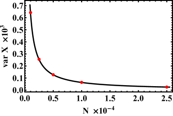
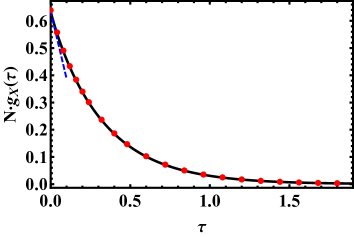
Figure 1 (top panel) compares this theoretical prediction with the variance of the COM, measured in Monte-Carlo simulations at different (see the Appendix for a brief description of the simulation algorithm). Figure 1 (bottom panel) compares the theoretically predicted covariance , Eq. (30), with the covariance measured in the simulations at and different . An excellent agreement is observed in both cases.
The scaling of the variance of the COM is to be expected from the law of large numbers. It also reflects the fact that large-scale hydrodynamic modes (with wavelengths comparable to the swarm size) dominate the contribution to the variance. We will encounter quite a different situation in the next section, which deals with fluctuations of the swarm radius .
V Fluctuations of the swarm radius
Averaging Eq. (26) over the noise, we obtain . Therefore, at least to the accuracy of the linear theory in , we have . The covariance of is given by
| (38) |
It is convenient to calculate the contributions to from the branching noise and from the noise of Brownian motion separately. Therefore we define , where
| (39) |
and . We can write
| (40) | |||||
Then, using Eq. (39) and performing the averaging, we obtain
| (41) |
where
| (42) | |||||
and
| (43) |
Again, the infinite sums over can be evaluated exactly with “Mathematica”, leading to the expression
| (44) |
where
| (45) |
for both and . Somewhat surprisingly, the branching noise and the noise of the Brownian motion give identical contributions to the covariance of . Therefore,
| (46) |
For the infinite sum over in Eq. (46) converges. In particular, the long-time decay of with is again purely exponential, , with the same ground state eigenvalue as for the COM.
But what happens at ? The large- asymptotic of from Eq. (45) is
| (47) |
Therefore, at the sum over in Eq. (46) diverges logarithmically at , implying an infinite variance. On the other hand, our Monte Carlo simulations (see below) clearly show a finite variance of . How to resolve this paradox?
Let us return to the covariance and recall that the Langevin description, which we adopted here as an approximation to the microscopic model, is applicable only at “macroscopic” times . Since the divergence of as is only logarithmical, we can introduce a cutoff at in the hope to obtain correct result for the variance of with logarithmic accuracy. Therefore, we proceed in the following way. For we use the large- asymptotic (47) of and replace the summation over in Eq. (46) by integration. This gives
| (48) |
where is the incomplete Gamma function. In fact, we must use the asymptotic of Eq. (48), which leads us to
| (49) |
The logarithmic growth of correlations of with a decrease of the time difference is a noticeable phenomenon. In the frequency space it corresponds to a noise. The noise has been observed in a plethora of physical and biological systems 1fnoise , and its appearance in the fluctuations of is unexpected.
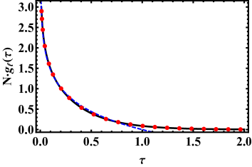
Now we can evaluate the variance of by introducing a cutoff in Eq. (49) at . We obtain, with logarithmic accuracy,
| (50) |
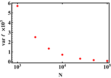
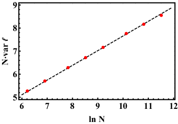
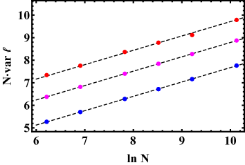
This result is markedly different from Eq. (37) by the presence of the large logarithmic factor , and this result is fully supported by our Monte-Carlo simulations of the microscopic model. Figures 2 and 3 show the simulation results for the fluctuations of , and compare them with theoretical predictions (46), (49) and (50). As one can see from the bottom panel of Fig. 2, the slope of the straight line, predicted by Eq. (50), agrees very well with the simulations. To eliminate the offset, we introduced a single adjustable offset parameter . It corresponds to a numerical factor under the logarithm which is beyond the logarithmic accuracy of Eq. (50).
VI Summary and Discussion
We studied analytically and numerically fluctuations of a swarm of Brownian bees in the limit of large but finite . We focused on two fluctuating quantities: the COM of the swarm and the swarm radius . We employed a first-principles Langevin equation for this system, linearized it around the deterministic steady state solution, and calculated the two-time covariances of and . As we found, the variance of behaves “normally”: it scales as as to be expected from the law of large numbers. But the variance of the swarm radius exhibits an anomalous scaling . This anomaly is caused by significant contributions to the variance from all spatial scales: from scales comparable to the swarm size down to the scale of a narrow region near the edges of the swarm where only a few bees are present. We have also shown that, at high but not too high frequencies, the power spectrum of the fluctuations of exhibits the noise. Our Monte-Carlo simulations of the microscopic system are in good agreement with theory.
A generalization to higher dimensions is especially interesting for the fluctuations of the swarm radius . One should expect that a small fraction of particles near the (circular or spherical) swarm boundary give a significant contribution to the variance of in higher dimensions as well. Furthermore, in all dimensions, the average steady-state particle flux to the boundary is the same (and equal to ). Therefore, the deterministic steady-state particle density behaves in a universal way near the swarm boundary. Does this universality lead to a similar behavior of the variance of vs. in different dimensions? Figure 4 depicts the results of our Monte Carlo simulations for and , where we measured the variance of at different . For comparison, also shown is the variance of for . Amazingly, as one can see from the figure, the slope of the straight line vs. , predicted by Eq. (50) for , holds for and as well. This remarkable coincidence certainly deserves a closer look at via an extension of our analytical calculations to higher dimensions.
It is instructive to compare the Brownian bees model with stochastic models, describing “pulled” reaction fronts propagating into an unstable empty state. The best known example of such models is the stochastic Fisher-Kolmogorov-Petrovsky-Piskunov (F-KPP) equation. The velocity of a stochastic F-KPP front fluctuates around its mean value, and the variance of these fluctuations scales as , where is the typical number of particles in the front region Derridaetal . This F-KPP anomaly is much stronger than the one in the Brownian bees model. This is because the F-KPP front velocity fluctuations are solely determined by a small fraction of particles located at the leading edge of the front Derridaetal .
In conclusion, we should remind the reader that the Langevin equation provides an accurate description only of typical, small fluctuations of reacting and diffusing systems of particles. Therefore, our present work is limited to typical fluctuations of the Brownian bees. It would be very interesting, and challenging, to also study large deviations of and , which correspond to the distribution tails of these quantities. Large deviations of persistent fluctuations of have been recently addressed in Ref. MS2021 by employing the optimal fluctuation method which bypasses the Langevin description.
Acknowledgments
We are grateful to N. R. Smith for useful discussions. The research of M.S. and B.M. was supported by the Israel Science Foundation (grant No. 1499/20). The research of P.S. was supported by the project “High Field Initiative” (CZ.02.1.01/0.0/0.0/15_003/0000449) of the European Regional Development Fund.
Appendix A Monte-Carlo simulations
We performed continuous-time Monte-Carlo simulations (see e.g. Ref. MCbook ) of the microscopic model. The small time intervals between two consecutive binary branching events were drawn from the exponential distribution with rate parameter . During these time intervals the particle positions were advanced according to the Brownian motion, given by the normal distribution , where is the particle’s initial position, and .
Next, one particle is chosen randomly, from the uniform distribution, to be the particle which is about to branch. The particle farthest from the origin is then relocated to the position of the chosen particle. This is equivalent to the removal of the farthest particle because of the birth of a “new” particle. This process can be thought of as relabeling the particles.
The measurements were performed, after the system reached a steady state, at fixed time steps . The simulation time was chosen to be sufficiently large, so that the precision of all measurements is at least within with confidence.
References
- (1) H.P. McKean, Comm. Pure Appl. Math. 28, 323 (1975).
- (2) M.D. Bramson, Mem. Am. Math. Soc. vol. 44 (285) (1983).
- (3) É. Brunet and B. Derrida, EPL 87, 60010 (2009); J. Stat. Phys. 143, 420 (2011).
- (4) A. H. Mueller and S. Munier, Phys. Rev. E 90, 042143 (2014).
- (5) K. Ramola, S. N. Majumdar, and G. Schehr, Phys. Rev. Lett. 112, 210602 (2014); Chaos, Solitons and Fractals 74, 79 (2015); Phys. Rev. E 91, 042131 (2015).
- (6) B. Derrida, B. Meerson and P. V. Sasorov, Phys. Rev. E 93, 042139 (2016).
- (7) G. Jona-Lasinio, C. Landim, and M. E. Vares, Probab. Theory Relat. Fields 97, 339 (1993).
- (8) G. Basile and G. Jona-Lasinio, Int. J. Mod. Phys. B 18, 479 (2004).
- (9) T. Bodineau and M. Lagouge, J. Stat. Phys. 139, 201 (2010).
- (10) P. I. Hurtado, A. Lasanta, and A. Prados, Phys. Rev. E 88, 022110 (2013).
- (11) B. Meerson, J. Stat. Mech. 2015, 05004.
- (12) J. Berestycki, É. Brunet, J. Nolen, and S. Penington, arXiv:2006.06486.
- (13) J. Berestycki, É. Brunet, J. Nolen, and S. Penington, arXiv:2005.09384.
- (14) B. Meerson and P. Sasorov, Phys. Rev. E 103, 032140 (2021).
- (15) É. Brunet, B. Derrida, A. H. Mueller and S. Munier, Europhys. Lett., 76, 1 (2006).
- (16) É. Brunet, B. Derrida, A. H. Mueller and S. Munier, Phys. Rev. E 76, 041104 (2007).
- (17) J. Bérard and J.-B. Gouéré, Comm. Math. Phys. 298, 323 (2010).
- (18) R. Durrett and D. Remenik, Ann. Probab. 39, 2043 (2011).
- (19) J. Berestycki, N. Berestycki, and J. Schweinsberg, Ann. Probab. 41, 527 (2013).
- (20) P. Maillard, Probab. Theory Related Fields 166, 1061 (2016).
- (21) N. Berestycki and L. Z. Zhao, Ann. Appl. Probab. 28, 651 (2018).
- (22) A. De Masi, P. A. Ferrari, E. Presutti and N. Soprano-Loto, in “Stochastic Dynamics out of Equilibrium”, Springer Proc. Math. Stat., vol. 282, p. 523 (Springer, Cham, 2019).
- (23) L. Addario-Berry, J. Lin, and T. Tendron, arXiv:2006.04743.
- (24) In the variant of the Brownian bees model, considered in Ref. ABLT , one removes, upon branching, the particle farthest from the center of mass of the system.
- (25) N. G. van Kampen, Stochastic Processes in Physics and Chemistry (North-Holland, Amsterdam, 2001).
- (26) C. W. Gardiner, Handbook of Stochastic Methods (Springer, Berlin, 2004).
- (27) H. Spohn, Large Scale Dynamics of Interacting Particles (Springer-Verlag, New York, 1991).
- (28) P. H. Handel and A. L. Chung, Noise in Physical Systems and Fluctuations (AIP, New York, 1993).
- (29) É. Brunet, B. Derrida, A. H. Mueller, and S. Munier, Phys. Rev. E 73, 056126 (2006).
- (30) D. P. Kroese, T. Taimre and Z. I. Botev, Handbook of Monte Carlo Methods, Wiley Series in Probability and Statistics (John Wiley and Sons, New York, 2011).