Optimizing for Diversity

Optimizing for Strategy Diversity in the Design of Video Games

Oussama Hanguir Industrial Engineering and Operations Research, Columbia University, New York, NY 10027, oh2204@columbia.edu Will Ma Graduate School of Business, Columbia University, New York, NY 10027, wm2428@gsb.columbia.edu Christopher Thomas Ryan UBC Sauder School of Business, University of British Columbia, Vancouver, BC, Canada, V6T 1Z2, chris.ryan@sauder.ubc.ca

We consider the problem of designing video games (modeled here by choosing the structure of a linear program solved by players) so that players with different resources play diverse strategies. In particular, game designers hope to avoid scenarios where players use the same “weapons” or “tactics” even as they progress through the game. We model this design question as a choice over the constraint matrix $A$ and cost vector $c$ that seeks to maximize the number of possible supports of unique optimal solutions (what we call loadouts) of Linear Programs $\max\{c^{\top}x\mid Ax\leq b,x\geq 0\}$ with nonnegative data considered over all resource vectors $b$. We provide an upper bound on the optimal number of loadouts and provide a family of constructions that have an asymptotically optimal number of loadouts. The upper bound is based on a connection between our problem and the study of triangulations of point sets arising from polyhedral combinatorics, and specifically the combinatorics of the cyclic polytope. Our asymptotically optimal construction also draws inspiration from the properties of the cyclic polytope. Our construction provides practical guidance to game designers seeking to offer a diversity of play for their plays.

video game design, linear programming, triangulations, cyclic polytope

1 Introduction

In this paper, we formulate the problem of designing linear programs that allow for diversity in their optimal solutions. This setting is motivated by video games, in particular, the design of competitive games where players optimize their strategies to improve their in-game status. For such games, a desideratum for game designers is for optimizing players to play different strategies at different stages of the game.

Let us first informally define the problem that we study. A more careful definition is given in the following subsections. We interpret the player’s problem as solving a Linear Program of the form $\max\{c^{\top}x\mid Ax\leq b,x\geq 0\}$. Players at different stages of the game have different resource vectors $b$. The columns of $A$ correspond to the tools that the player can use in the game. We call a subset of these tools (represented by subsets of the columns of $A$) a loadout if they correspond to the support of an optimal solution $x^{*}$ to the linear program $\max\{c^{\top}x\mid Ax\leq b,x\geq 0\}$ for some resource vector $b$. The support of a vector corresponds to a selection of the available tools, forming a strategy for how the player approaches the game given available resources. We assume that the game designer is able to choose $A$ and $c$. We refer to this choice as the design of the game. We measure the diversity of a design as the number of possible loadouts that arise as the resource vector $b$ changes. The game designer’s problem is to find a design that maximizes diversity. A solution to this problem is then able to meet the game designer’s goal of finding a design where optimizing players employ as many different loadouts as possible as the game evolves and player resources change. In the next subsection, we also provide a concrete game example to ground some of these concepts.

1.1 Video game context and formal problem definition

Video games are both the largest and fastest-growing segment of the entertainment industry, to the extent that in 2020, the video game industry surpassed movies and North American sports combined in revenue (Witkowski 2021). In gaming, as in related domains, key design aspects that affect player enjoyment include story, pacing, challenge level, and game mechanics. In this paper, we focus on game mechanics, carefully designing the structure of the set of tools available to the player as the key intervention to drive enjoyment.

For many video games, engaged players aim to pick the best strategy available to conquer the challenges they face. Often the key strategic decision is to select the best set of tools (often, weapons) to use to meet challenges. Players have limited in-game resources and face constraints (size of weapons, a limit on the number of weapons of some type, etc.) when selecting their strategy. These decisions, therefore, can be modeled as constrained optimization problems.

To make this discussion concrete, consider the following fictional game. In RobotWar, we control a sci-fi robot to drive into battle against other robots. As we play the game, we accrue and manage experience points (XP). Before each battle, we pick the combination of weapons and equipment our robot takes into battle. There are different types of weapons including short-range (sabers, shotguns, etc.) and long-range (sniper cannon, explosive missiles, etc.). Weapons can be bought with experience points, and there are capacity constraints on the sizes of the weapons carried (including ammunition) that is proportional the amount of XP invested in them. Every weapon has an initial damage (per usage) that it can deal to the opponent, but we can increase the damage of a weapon by investing additional XP. By winning more battles, we get more XP and increase the robot’s capacity to hold more weapons.

Before each battle, a player picks the weapons that will be used, as well as how much XP is invested into each weapon. Assume that we are at a given stage of the game with a fixed amount of XP and fixed capacities. We want our robot to have the highest possible total damage value. We can compute the combination of weapons that maximizes the total damage by solving a linear program with decision variables representing how much XP to invest in each weapon. The set of weapons that the player invests a positive amount of XP into is called the player’s loadout. In the context of RobotWar, the key strategic choice is selecting a loadout. Note that a loadout refers to the combination of weapons and not the amount of XP invested in each weapon. If the same combination of weapons is adopted but with different allocations of XP, then in the two situations we have used the same loadout.

The previous example shows how a video game can be designed so that determination of an optimal loadouts can be done through optimization. In the next subsection, we present real-life video game settings where players, in fact, use optimization to form their strategies.

In light of the loadout decisions of players, game designers may ponder the following question: how to set the constraints of the game and the attributes of the tools so that the number of optimal loadouts across all possible resource states is maximized? In other words, the game designer may want to set the game up in such a way that as the resources of the players evolve, the optimal loadouts change. A desire to maximize the number of optimal loadouts is motivated by the fact that video games can get boring when they are too repetitive with little to no variation (Schoenau-Fog et al. 2011). It is considered poor game design if a player can simply “spam” (i.e., repeatedly use) one strategy to progress easily through a game without needing to adjust their approach.

In our study, we assume that our game design question can be captured by a linear program. This is justified as follows. Consider a game that has $n$ available tools. The player has a decision variable $x_{i}$ for each tool $i$, which represents “how much” of the tool the player employs. We put “how much” in quotations because there are multiple interpretations of what this might mean. In the RobotWar example, $x_{i}$ denotes the amount of XP invested in weapon $i$. The more XP invested, the more the weapon can be used. This can be interpreted as a measure of “ammunition” or “durability”. Let $c\in\mathbb{R}_{\geq 0}^{n}$ denote the vector of benefits that accrue from using the various tools. That is, one unit of tool $i$ yields a per-unit benefit of $c_{i}$. In the RobotWar example, $c_{i}$ represents the damage dealt to the opponent by weapon $i$ per unit of XP invested in weapon $i$.

The player must obey a set of $m$ linear constraints when selecting tools. These constraints are captured by a matrix $A\in\mathbb{R}_{\geq 0}^{m\times n}.$ These constraints include considerations like a limit on the number of coins or experience points that the player has, a limit on the capacity (weight, energy, etc.) of the tools that can be carried, etc. A vector $b\in\mathbb{R}_{\geq 0}^{m}$ represents the available resources at the disposal of the player and forms the right-hand sides of the set of constraints. In the RobotWar example, there are natural constraints corresponding to total available XP and capacities for the various weapons.

For a fixed game design $(A,c)$ and resource vector $b$, players solve the linear program

$$LP(A,c,b):\qquad\max\{c^{\top}x\mid Ax\leq b,x\geq 0\},$$ (1)

where $c$, $A$, and $b$ all have nonnegative data. If $x$ is the optimal solution of $LP(A,c,b)$, we define the support of $x$ as $\operatorname{supp}(x)\triangleq\{i\in\{1,\ldots,n\}\mid x_{i}>0\}.$ If $x$ is the unique optimal solution of $LP(A,c,b)$, then we call $\operatorname{supp}(x)$ an optimal loadout (or simply, a loadout) of design $(A,c)$.

For fixed $n$ and $m$, the loadout maximization problem is to choose the vector $c$ and matrix $A$ that maximize the total number of loadouts of the design $(A,c)$. That is, the goal is to design benefits for each tool (the vector $c$) and limitations on investing in tools (the matrix $A$) so that the linear programs $LP(A,c,b)$ have as many possible supports of unique optimal solutions as possible, as $b$ varies in $\mathbb{R}^{m}$.

Note that the loadout maximization problem is a natural question to ask about Linear Programs in general. Indeed, much of our analysis will treat the problem in general without carrying too much of the video game interpretation. However, it is important to stress the interpretation of this problem grounded in the video game context. We highlight three key elements of this interpretation:

• We are interested in loadouts, corresponding to supports of optimal solutions, but not in the values of the solutions themselves. This is motivated by our desire to maximize diversity; two solutions that have the same support and use the same set of tools but in different proportions are considered variations of the same strategy and not a different strategy.

• We restrict attention to unique optimal loadouts. If we considered maximizing the number of supports of all (even non-unique) optimal solutions, this leads to degenerate cases that should be excluded. As a trivial example, in any design with $c=0$, every loadout is optimal as they all give rise to the same objective value of $0$. This is not a desirable design in practice because there is no strategy involved for the player in designing their loadout. That fact we consider unique optimal solutions can also be motivated by the fact that it is helpful for a game designer to be able to predict the best strategy of a player given their resources. This can be especially useful in online role-playing video games and survival games where players fight computer-controlled enemies and so knowing a player’s optimal strategy helps balance the difficulty of the environment.

• We only count the supports of unique optimal solutions and ignore the supports of non-optimal solutions. A reason for this has already been mentioned, optimal behavior is easy to predict whereas “non-optimal behavior” is difficult to anticipate. Furthermore, in many modern video games that have a “freemium” revenue model, most of the revenue comes from dedicated “hardcore” players, who are more likely to optimize in order to continue their in-game progress. By restricting attention to optimal player behavior in the design problem, the game designer makes decisions for its highest tier of revenue-generating players.

1.2 Some illustrative examples

We now turn to a consideration of some real games where the loadout maximization problem has relevance in practice. Although these examples may not perfectly fit the linear model that we study here in every aspect, they nonetheless share the same essential design and speak to the tradeoffs of interest.

Consider, for example, the MOBA (Multiplayer Online Battle Arena) genre that has become increasingly popular in past years. In the MOBA game SMITE, for example, players take control of deities from numerous pantheons across the world. Teams of deities work together to destroy objects in enemy territory, while defending their own territory against an enemy team trying to do the same. The main source of advantage is to purchase tools that enhance the attributes of the deities. These attributes include power, attack speed, lifesteal (percentage of damage dealt to enemy deities that is returned back to the player as health), and critical strike chance (the chance of an attack dealing double the damage that it would normally do). In this game, one can (and some players actually do (Knight 2015)) use linear programming to model the tools to buy and decide which ones will give the best advantage, while at the same time keeping costs down. Game designers can, accordingly, anticipate the decision-making procedures of players and select the various attributes of the tools and their prices to promote diversity of gameplay.

Another example of using linear programming to compute an optimal strategy is in the game Clash of Clans. In this game, players fortify their base with buildings to obtain resources, create troops, and defend against attacks. Players put together raiding parties to attack other bases. Linear programming can be used to determine the best combination of characters in a raiding party, with constraints on the training cost of warriors (measured in elixir, a resource that the player mines and/or plunders) as well as space in the army camps to house units (Knight 2014).

While these examples show how maximizing behavior among players can be effectively modeled as linear programs, there is also evidence that game designers are interested in maximizing diversity using optimization tools. For example, veteran game designer Paul Tozour presents the problem of diversity maximization in a series of articles on optimization and game design on Gamasutra, a video game development website (Tozour 2013). In an article in that series, Tozour describes the fictional game of “SuperTank” (similar to our fictional RobotWar) to show how optimization models can be used to design the attributes of available weapons that lead to varied styles of play. Tozour makes a strong case throughout his series of articles for using optimization tools, stating that game designers

…might be able to use automated optimization tools to search through the possible answers to find the one that best meets their criteria, without having to play through the game thousands of times.

1.3 Our contributions

We initiate the study of the loadout maximization problem. Our first contribution in the paper is to establish a link between the loadout maximization problem and the theory of polyhedral subdivisions and triangulations. In particular, for a fixed design $(A,c)$, the theory of triangulations offers a nice decomposition (or triangulation) of the cone generated by the columns of the constraint matrix $A$. This decomposition depends on the objective vector $c$. We show that for a fixed design $(A,c)$, the loadouts can be seen as elements of this decomposition. This allows us to use a set of powerful tools from the theory of triangulations to prove structural results on the loadouts of a design.

Our second contribution is to show a non-trivial upper bound on the number of loadouts of any design. The upper bound involves an interesting connection to the faces of the so-called cyclic polytope, a compelling object central to the theory of polyhedral combinatorics. We also show that this upper bound holds when the constraints of the linear program are equality constraints.

The third contribution of this paper is to present a construction of a design $(A,c)$ with a number of loadouts that asymptotically matches the above upper bound. Furthermore, for cases with few constraints, we present optimal constructions that exactly match the upper bound. Our constructions provide practical insights that game designers can use to balance the tools available in the game, with the hope of increasing strategy diversity.

Outline of sections. In Section 2, we cleanly state all of our results, sketch their proofs, and illustrate their intuition on small examples, without formally defining all terminology and definitions related to linear programming and triangulations. These formal definitions can be later found in Section 3. Our upper bound results are derived in Section 4, while our asymptotically optimal constructions are presented in Section 5.

1.4 Related work

Video game research in the management sciences. The increasing popularity of video games and the growth of the global video game market has led to a considerable surge in the study of video game related problems in operations management, information systems, and marketing. There have been several studies on advertising in video games. Turner et al. (2011) study the in-game ad-scheduling problem. Guo et al. (2019b) and Sheng et al. (2020) study the structure of “rewarded” advertising where players are incentivized to watch ads for in-game rewards. Generally, these rewards come in the form of virtual currencies whose value is fixed by the game designer. Guo et al. (2019a) study the impact of selling virtual currency on players’ gameplay behavior, game provider’s strategies, and social welfare. Another significant research direction concentrates on studying “loot boxes” in video games, where a loot box is a random allocation of virtual items whose contents are not revealed until after purchase, and that is sold for real or in-game money. Chen et al. (2020) study the design and pricing of loot boxes, while Ryan et al. (2020) study the pricing and deployment of enhancements that increase the player’s chance of completing the game.

Chen et al. (2017) and Huang et al. (2019) study the problem of in-game matchmaking to maximize a player’s engagement in a video game. Jiao et al. (2020) investigate whether the seller should disclose an opponent’s skill level when selling in-game items that can increase the win rate.

Other streams of works focused on how video game data can be used to study player behavior. Nevskaya and Albuquerque (2019) empirically explore the impact of different in-game policies that can limit excessive engagement of players in games, while Kwon et al. (2016) uses individual-level behavioral data to study the evolution of player engagement post-purchase.

Optimization Theory and Parametric Programming. Our work is closely related to parametric linear programming, which is the study of how optimal properties depend on parameterizations of the data. The study of parametric linear programming dates back to the work of Saaty and Gass (1954), Mills (1956), Williams (1963), and Walkup and Wets (1969) in the 1950s and 1960s. In parametric programming, the objective is to understand the dependence of optimal solutions on one or more parameters; that is, on the entries of $A$, $b$, and $c$. Our work is novel in the sense that the objective is to understand the structure of the supports of optimal solutions by fixing $A$ and $c$ and having $b$ vary in $\mathbb{R}^{m}_{\geq 0}$. To the best of our knowledge, this question has not previously been studied in the literature.

2 Statement of the main results

In this section, we state our main results. To make these statements precise, we require some preliminary definitions. Let $[k]$ denote the set $\{1,\ldots,k\}$ for any positive integer $k$. Using this notation, we can define the support of $x\in\mathbb{R}^{n}_{\geq 0}$ as $\operatorname{supp}(x)=\{j\in[n]\mid x_{j}>0\}$. For a matrix $A\in\mathbb{R}^{m\times n}_{\geq 0}$, the $(i,j)$th entry is denoted $a_{ij}$ for $i\in[n]$ and $j\in[m]$, the $j$th column is denoted $A_{j}$ for $j\in[n]$, and the $i$th row is denoted $a_{i}$ (where $a_{i}$ is a column vector) for $i\in[m]$. For a column vector $y\in\mathbb{R}^{m}$, $y^{\top}A_{j}$ denote the scalar product of $y$ and column $A_{j}$, i.e., $y^{\top}A_{j}=\sum_{i=1}^{m}y_{i}a_{i,j}$.

Recall the definition of the linear program $LP(A,b,c)$ in 1. As mentioned in the introduction, we are interested in the unique optimal solutions of the design $(A,c)$. For simplicity, we simply call these the loadouts of design $(A,c)$; that is, $L\subseteq[n]$ is a loadout of design $(A,c)$ if there exists a nonnegative resource vector $b\in\mathbb{R}^{m}_{\geq 0}$ such that $LP(A,c,b)$ has a unique optimal solution $x^{*}$ with $\operatorname{supp}(x)=L$. We say that loadout $L$ is supported by resource vector $b$. If $|L|=k$ then we say $L$ is a $k$-loadout. Given a design $(A,c)$ and an integer $k\in[m]$, let $\mathcal{L}^{k}(A,c)$ denote the set of all $k$-loadouts of design $(A,c)$. The set of all loadouts of any size is $\mathcal{L}(A,c)\triangleq\cup_{k=1}^{n}\mathcal{L}^{k}(A,c)$.

Using this notation, we can restate the loadout optimization problem. Given dimensions $n$ and $m$ and integer $k\leq n$, the $k$-loadout optimization problem is

$$\max\{|\mathcal{L}^{k}(A,c)|\mid A\in\mathbb{R}^{m\times n},c\in\mathbb{R}^{n},A\text{ and }c\text{ are nonnegative}\}. \text{L}_{k}$$ ()

We can assume without loss of generality that the linear programs $LP(A,c,b)$ are bounded and thus possess an optimal solution because otherwise there is no optimal solution and, therefore, no loadout.

Given that a loadout corresponds to the support of a unique solution of a linear program, any optimal solution with support size greater than $m$ cannot be unique. Therefore, the number of $k$-loadouts when $k>m$ is always equal to zero. This leads us to consider the optimization problems $\text{L}_{k}$ only for $k\in\{1,\ldots,\min(m,n)\}.$ For convenience, we will avoid the trivial case of $k=1$ where the optimal number of loadouts is $\min(m,n)$. A final case we eliminate immediately is when $\min(m,n)=n$, i.e. $m\geq n$. In this case, a trivial design is optimal. By setting $A=I_{n}$ to be the identity matrix of size $n$, and $c=(1,\ldots,1)$, we ensure that for $k\in[1,n]$, every one of the $\binom{n}{k}$ subsets is a loadout (see Lemma 8.1 in the appendix).

In summary, we proceed without loss under the assumption that $n>m\geq k\geq 2$.

2.1 The Cyclic Polytope

All of our bounds are intimately related to the number of faces on the cyclic polytope, which is formally defined in Section 3. A remarkable aspect of the cyclic polytope is that for $n>m\geq 2$, the cyclic polytope $\mathcal{C}(n,m)$ simultaneously maximizes the number of $k$-dimensional faces for all $k=0,\ldots,m-1$ among $m$-dimensional polytopes over $n$ vertices, a property known as McMullen’s Upper Bound Theorem (McMullen 1970). The number of $k$-dimensional faces on $\mathcal{C}(n,m)$ is given by the formula

$$f_{k}(\mathcal{C}(n,m))=\sum\limits_{\ell=0}^{\lfloor m/2\rfloor}\binom{\ell}{m-k-1}\binom{n-m+\ell-1}{\ell}+\sum\limits_{\ell=\lfloor m/2\rfloor+1}^{m}\binom{\ell}{m-k-1}\binom{n-\ell-1}{m-\ell}.$$

When $k=m-1$, this simplifies to

$$f_{m-1}(\mathcal{C}(n,m)) =\binom{n-\lceil m/2\rceil}{\lfloor m/2\rfloor}+\binom{n-\lfloor m/2\rfloor-1}{\lceil m/2\rceil-1}.$$

As an illustration of these formulas, suppose $m=3$. The formulas evaluate to

$$f_{2}(\mathcal{C}(n,3)) =\binom{n-2}{1}+\binom{n-2}{1} = 2n-4$$ (2)

$$f_{1}(\mathcal{C}(n,3)) =1\binom{n-3}{1}+2\binom{n-3}{1}+3\binom{n-4}{0} = 3n-6$$ (3)

$$f_{0}(\mathcal{C}(n,3)) =\binom{2}{2}\binom{n-3}{1}+\binom{3}{2}\binom{n-4}{0} = n.$$

To check that this is correct, note that $f_{0}(\mathcal{C}(n,3))$ should be $n$ by definition. Meanwhile, we remark that the cyclic polytope is a simplicial polytope, i.e. all of its $(m-1)$-dimensional faces are the convex hull of exactly $m$ points. When $m=3$, this translates to all of its facets being triangles. Therefore, $2f_{2}(\mathcal{C}(n,3))=3f_{1}(\mathcal{C}(n,3))$, since every edge is contained in exactly 2 triangles and every triangle contains exactly 3 edges. In conjunction with Euler’s immortal formula $f_{2}(\mathcal{C}(n,3))+f_{0}(\mathcal{C}(n,3))=f_{1}(\mathcal{C}(n,3))+2,$ one can uniquely express $f_{2}(\mathcal{C}(n,3)),f_{1}(\mathcal{C}(n,3))$ as a function of $n$ for simplicial polytopes in 3 dimensions, which indeed can be checked to equal respective expressions 2 and 3 above. In higher dimensions, simplicial polytopes can have different numbers of faces for each dimension, but they can never surpass the number on the cyclic polytope for that dimension.

2.2 Statements of Main Results

Theorem 2.1

Fix positive integers $n,m,k$ with $n>m\geq k\geq 2$. Then the number of $k$-loadouts for any design $(A,c)$ with $A\in\mathbb{R}^{m\times n}$ and $c\in\mathbb{R}^{n}$ satisfies

$$|\mathcal{L}^{k}(A,c)| \leq f_{k-1}(\mathcal{C}(n+1,m))-\binom{m}{k-1}.$$ (4)

We note that the trivial upper bound on the number of $k$-loadouts in a design with $n$ tools is $\binom{n}{k}$. When $m<n$, the RHS of (4) will always be smaller than this trivial upper bound, which shows that having a limited number of resource types in the game does indeed prevent all subsets of tools from being viable.

Theorem 2.2

Fix positive integers $n,m,k$ with $n>m\geq k\geq 2$. Then we can provide a family of explicit designs $(A,c)$ with $A\in\mathbb{R}_{\geq 0}^{m\times n}$ and $c\in\mathbb{R}_{\geq 0}^{n}$ that satisfy

$$|\mathcal{L}^{k}(A,c)| \geq\begin{cases}f_{k-1}(\mathcal{C}(n,m))&\text{if $k<m/2$}\\ f_{k-1}(\mathcal{C}(n,m))/2&\text{if $k\geq m/2$ and $m$ is odd, or $k=m/2$ and $m$ is even}\\ f_{k-1}(\mathcal{C}(n,m))/4&\text{if $k>m/2$ and $m$ is even}.\end{cases}$$

The constructions from Theorem 2.2 are always within a 1/4-factor of being optimal asymptotically as $n\to\infty$ because it is known (see Lemma 9.1 in Appendix 9 for a formal proof) that

$$\lim_{n\to\infty}\frac{f_{k-1}(\mathcal{C}(n,m))}{f_{k-1}(\mathcal{C}(n+1,m))}=1.$$

Theorem 2.3

For $n>m=3$, we can provide a family of explicit designs $(A,c)$ with $A\in\mathbb{R}_{\geq 0}^{m\times n}$ and $c\in\mathbb{R}_{\geq 0}^{n}$ that satisfy $|\mathcal{L}^{3}(A,c)|\geq 2n-5$ and $|\mathcal{L}^{2}(A,c)|\geq 3n-6$.

Theorem 2.4

For $n>m=2$, we can provide a family of explicit designs $(A,c)$ with $A\in\mathbb{R}^{m\times n}$ and $c\in\mathbb{R}^{n}$ that satisfy $|\mathcal{L}^{2}(A,c)|\geq n-1.$

The constructions from Theorem 2.3 and Theorem 2.4 are exactly tight; it can be checked that they match the upper bound expression from Theorem 2.1 when evaluated at $m=3$ and $m=2$. The proofs of both theorems are deferred to Appendix 12.

Example of construction from Theorem 2.2 and intuition. Table 1 shows an example of the asymptotically optimal construction for $m=4$ and $n=6$. Our construction provides a pattern that game designers can follow to diversify loadouts on a set of tools $1,\ldots,n$, by having two types of constraints. The first type of constraints (rows 1 and 3) accords more importance to tools with big indices (because these tools have lower costs to rows 1 and 3) while the second type of constraints (rows 2 and 4) give more advantage to tools with a small index (because these tools have lower costs to rows 2 and 4). This “tension” between the two types of constraints ensures that a given combination of tools cannot be optimal for too many resource vectors. This captures the rough intuition that a game with an overpowered tool (meaning one that is more useful than the others but also not significantly “cumbersome” to limit its use) leads to uniform strategies among players. In other words, for diversity, all tools should have strengths and weaknesses.

Furthermore, among the constraints of the same type, the resource requirements of tools either monotonically increase or monotonically decrease along the rows. The implication of this is as follows. Consider the tool corresponding to the first column in Table 1. This tool is cheapest with respect to the first and third resources and the most expensive with respect to the second and fourth. Thus, any time the player has an excess of resources 2 and 4, she will certainly use the first tool. However, as soon as one of those resources is constrained, it is tempting to jettison the first tool. This monotone structure heightens the sensitivity of the structure of optimal solutions to changes in the resource vector. Practically speaking, this means that tools that are very powerful in some dimensions must also have significant weaknesses to ensure variety of play. A concrete example of this is the “rocket launcher” in first-person shooters, which is typically the most powerful weapon but suffers from having the most expensive ammunition. This can be captured in our Table 1 construction by scaling any of the columns to have higher reward but also higher cost.

$c$	1	1	1	1	1	1
$A$	1	2	3	4	5	6
	$M-1^{2}$	$M-2^{2}$	$M-3^{2}$	$M-4^{2}$	$M-5^{2}$	$M-6^{2}$
	$1^{3}$	$2^{3}$	$3^{3}$	$4^{3}$	$5^{3}$	$6^{3}$
	$M-1^{4}$	$M-2^{4}$	$M-3^{4}$	$M-4^{4}$	$M-5^{4}$	$M-6^{4}$

Table 1: Example of our construction with $m=4$, $n=6$, and $M=6^{4}+1$.

2.3 Roadmap for proving Theorems 2.1 and 2.2

This subsection provides a high-level overview of our approach for establishing our upper and lower bounds. All the undefined terminology used here will be defined in more detail in later sections.

We prove our upper bound Theorem 2.1 using a sequence of transformations.

1. We first introduce the intermediate concept of an equality loadout problem that replaces the inequality constraint $Ax\leq b$ with an equality $Ax=b$. A $k$-equality loadout is a $k$-loadout in this revised problem. We show that for a fixed design $(A,c)$ and for every dimension $k$, the number of $k$-loadouts is less than the number of $k$-equality loadouts (Lemma 4.1).

2. This allows us to focus on proving an upper bound on the number of equality loadouts. Here, we can exploit the dual structure of the equality LP and prove that equality loadouts belong to a cell complex $\Delta_{c}(A)$ that is characterized by $A$ and $c$. Importantly, we show that loadouts correspond to simplicial cells in this cell complex (Lemma 4.4).

3. In turn, this allows us to, without loss of generality, assume that $\Delta_{c}(A)$ is a triangulation (as opposed to an arbitrary subdivision), of a cone in the positive orthant of $\mathbb{R}^{m}$ (Lemma 4.7).

4. We show that triangulations of cones in the positive orthant of $\mathbb{R}^{m}$ correspond to triangulations of points in the lower dimension $\mathbb{R}^{m-1}$ (Lemma 4.9).

5. Finally, we show that the simplices in this triangulation can be embedded into faces of a simplicial polytope in $\mathbb{R}^{m}$. Therefore, any upper bound on the number of faces of polytopes in $\mathbb{R}^{m}$ implies an upper bound on the number of loadouts. This allows us to invoke the “maximality” of the cyclic polytope with respect to its number of faces mentioned in Section 2.1. Therefore, the number faces of the cyclic polytope of dimension $m$ bounds the number of faces in a polytope of dimension $m$, and implies a bound on the number of equality loadouts. We also carefully count the number of extraneous faces added through our transformations, by invoking a bound on the minimal number of faces a polytope can have, which allows us to derive tight bounds for small values of $m$ (Lemma 4.10).

We remark that in the above proof, we needed to first map to triangulations in the lower dimension $\mathbb{R}^{m-1}$ and then later return to polytopes in the original dimension $\mathbb{R}^{m}$, in order to invoke McMullen’s Upper Bound. However, this required the introduction of a point at the south pole, which means that it is difficult for our upper bound to be tight for small values of $n$. Nonetheless, the introduction of this additional point is insignificant as $n\to\infty$. This is why we can prove asymptotic optimality.

To prove our complementing lower bound Theorem 2.2, we first explicitly provide our design $(A,c)$ in Section 5.1, which is also inspired by the cyclic polytope. Compared to the cyclic polytope, every even row of the matrix $A$ has been “flipped” (as previously observed in Table 1), for reasons that will become apparent in our proof, which we now outline.

1. First, we focus on the dual program of $LP(A,c,b)$ and present a sufficient condition (Definition 5.1) for loadouts in terms of dual variables (Lemma 5.2).

2. We show that by taking hyperplanes corresponding to the facets of the cyclic polytope in dimension $m$, one can attempt to construct dual variables that satisfy the sufficient condition (Lemma 5.4). Our aforementioned “flipping” of the even rows in $A$ is crucial to this construction of the dual variables. We show that as long as the facet of the cyclic polytope is of the “odd” parity, the constructed dual variables will indeed be sufficient (Lemma 5.7), and hence such a facet and all of the faces contained within it correspond to loadouts.

3. Therefore, to count the number of $k$-loadouts, we need to count the number of $(k-1)$-dimensional faces on a cyclic polytope in dimension $m$ that are contained within at least one odd facet. To the best of our knowledge, this is an unsolved problem in the literature. Nonetheless, using Gale’s evenness criterion we can map this to a purely combinatorial problem on binary strings (Lemma 5.8 and Lemma 5.10). Through some combinatorial bijections, we show that at worst a factor of 4 is lost when one adds the requirement that the $(k-1)$-dimensional face must be contained within at least one odd facet, with the factor improving to 2 if $m$ is odd (Corollary 5.20), and improving to 1 if $k$ is small (Corollary 5.16). These arguments form the cases in Theorem 2.2.

To summarize, both our upper and lower bounds employ the cyclic polytope, but through different transformations—projecting down to $\mathbb{R}^{m-1}$ and then lifting back up for the upper bound, and “flipping” even rows for the lower bound.

3 Preliminaries

We present terminology we use in the proofs of both Theorems 2.1 and 2.2. Additional terminology needed in the proof of only one of these results is found in the relevant sections.

A $d$-simplex is a $d$-dimensional polytope that is the convex hull of $d+1$ affinely independent points. For instance, a 0-simplex is a point, a 1-simplex is a line segment and 2-simplex is a triangle. For a matrix $A=(A_{1},\ldots,A_{n})$ of rank $m$, let $\operatorname{cone}(A)=\operatorname{cone}(\{A_{1},\ldots,A_{n}\})$ represent the closed convex polyhedral cone $\{Ax\mid x\in\mathbb{R}^{n}_{+}\}$. We use the notation $\operatorname{cone}(C)$ to denote the cone generated by the columns indexed by $C\subseteq[n]$. If $C\subseteq[n]$ is a subset of indices, the relative interior of $C$ is the relatively open (i.e., open in its affine hull) convex set

$$\operatorname{relint}_{A}(C)\triangleq\big{\{}\sum\limits_{j\in C}\lambda A_{j}\mid\lambda_{j}>0\mbox{ for all }j\in C,\mbox{ and }\sum\limits_{j\in C}\lambda_{j}=1\big{\}}.$$

A subset $F$ of polytope $P$ is a face if there exists $\alpha\in\mathbb{R}^{n}$ and $\beta\in\mathbb{R}$ such that $\alpha^{\top}x+\beta\leq 0$ for all $x\in P$ and $F=\{x\in P\mid\alpha^{\top}x+\beta\ =0\}$. If $\dim(F)=k$ then $F$ is called a $k$-dimensional face or $k$-face. The faces of dimensions 0, 1, and $\dim(P)-1$ are called vertices, edges, and facets, respectively. Furthermore, we say that $F$ is face of $C$, where $F,C\subseteq[n]$, when $\operatorname{cone}(F)$ is a face of $\operatorname{cone}(C)$. We define a polyhedral subdivision of $\operatorname{cone}(A)$ as follows.

Definition 3.1

Let $A=(A_{1},\ldots,A_{n})$ be a matrix of rank $m$. A collection $\mathscr{S}$ of subsets of $[n]$ is a polyhedral subdivision of $\operatorname{cone}(A)$ if it satisfies the following conditions:

• If $C\in\mathscr{S}$ and $F$ is a face of $C$, then $F\in\mathscr{S}$. (Closure Property)

• $\operatorname{cone}(\{1,\ldots,n\})\subset\bigcup\limits_{C\in\mathscr{S}}\operatorname{cone}(C)$. (Union Property)

• If $C,C^{\prime}\in\mathscr{S}$ with $C\neq C^{\prime}$, then $\operatorname{relint}_{A}(C)\cap\operatorname{relint}_{A}(C^{\prime})=\emptyset$. (Intersection Property)

If $\{j_{1},\ldots,j_{k}\}$ belongs a subdivision of $\operatorname{cone}(A)$, then the set of indices $\{j_{1},\ldots,j_{k}\}$ is called a cell of the subdivision, and if the cone is of dimension $k$, it is called a $k$-cell. We note that a polyhedral cone subdivision is completely specified by listing its maximal cells.

Next, we define a special subdivision of $\operatorname{cone}(A)$ as a function of the cost vector $c$. The cells of this subdivision map to the loadouts of the design $(A,c)$. For $A\in\mathbb{R}^{m\times n}_{\geq 0}$ and $c\in\mathbb{R}^{n}_{\geq 0}$, we define the polyhedral subdivision $\Delta_{c}(A)$ of $\operatorname{cone}(A)$ as a family of subsets of $\{1,\ldots,n\}$ such that $C\in\Delta_{c}(A)$ if and only if there exists a column vector $y\in\mathbb{R}^{m}$ such that $y^{\top}A_{j}=c_{j}$ if $j\in C$ and $y^{\top}A_{j}>c_{j}$ if $j\in\left\{1,\dots,n\right\}\setminus C$. In such a case, we say $C$ is a cell of $\Delta_{c}(A)$ and that $\Delta_{c}(A)$ is a cell complex. A cell $C\in\Delta_{c}(A)$ is simplicial if the column vectors $(A_{j})_{j\in C}$ are linearly independent. If all the cells of $\Delta_{c}(A)$ are simplicial, then we say $\Delta_{c}(A)$ is a triangulation. The maximum size of a simplicial cell is $m$. The next results shows that $\Delta_{c}(A)$ is indeed a polyhedral subdivision of $\operatorname{cone}(A)$. The proof is deferred to Appendix 7.

Proposition 1

$\Delta_{c}(A)$ is a polyherdal subdivision of $\operatorname{cone}(A)$.

Intuitively, we can think of the subdivision $\Delta_{c}(A)$ as follows: take the cost vector $c$, and use it to lift the columns of $A$ to $\mathbb{R}^{n+1}$ then look at the projection of the upper faces (those faces you would see if you “look from above”). This is illustrated in Example 3.2.

Example 3.2

Consider the following matrix and cost vectors

$$A=\begin{pmatrix}1/4&1/2&3/4\\ 1&1&1\end{pmatrix},\quad c_{1}=(2,2.125+\epsilon,2.25)\quad\mbox{ and }\quad c_{2}=(2,2.125-\epsilon,2.25),$$ (5)

where $\epsilon>0$ is a small constant. The corresponding subdivisions of $\operatorname{cone}(A)$ are

$$\Delta_{c_{1}}(A)=\big{\{}\{1,2\},\{2,3\},\{1\},\{2\},\{3\},\emptyset\big{\}}\ \ \mbox{ and }\ \ \Delta_{c_{2}}(A)=\big{\{}\{1,2,3\},\{1\},\{3\},\emptyset\big{\}}.$$

For example, to see that $\{1,2\}$ is a cell of $\Delta_{c_{1}}(A)$, we consider $y=(0.5+4\epsilon,1.875-\epsilon)$. One can verify that $y^{\top}A_{1}=c_{1}$ and $y^{\top}A_{2}=c_{2}$, while $y^{\top}A_{3}>c_{3}$. We observe that for the cost vector $c_{1}$, the cell $\{1,2\}$ is simplicial, while for $c_{2}$, the cell $\{1,2,3\}$ is not simplicial. See Figure 1 for a visualization of $\Delta_{c_{1}}(A)$ and $\Delta_{c_{2}}(A)$. $\triangleleft$

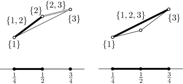
Figure 1: An illustration of the triangulations $\Delta_{c_{1}}(A)$ (left side of the figure) and $\Delta_{c_{2}}(A)$ (right side of the figure). In the figure, the third dimension (corresponding to the row of $1$’s in the matrix $A$ in 5) is suppressed since all objects are at the same height of $1$.

In our definition of simplicial cell, we mentioned that if all the cells in the subdivision $\Delta_{c}(A)$ are simplicial, then $\Delta_{c}(A)$ is called a triangulation. More generally, a triangulation of cones is a cone subdivision where all the cells are simplicial (the columns of every cell are linearly independent). We will also define the notion of triangulations of point configurations, which we define below.

Definition 3.3

Let $B=\{x_{1},\ldots,x_{n}\}$ be a point configuration (i.e., a finite set $B$ of points) in $\mathbb{R}^{n}$. A triangulation of $B$ is a collection $\mathcal{T}$ of simplices whose vertices are points in $B$, and whose dimension is the same dimension as the affine hull of $B$, with the following properties:

• If $C\in\mathcal{T}$ and $F\subseteq C$, then $F\in\mathcal{T}$. (Closure Property)

• $\operatorname{conv}(B)\subset\bigcup\limits_{C\in\mathcal{T}}\operatorname{conv}(C)$. (Union Property)

• If $C,C^{\prime}\in\mathcal{T}$ with $C\neq C^{\prime}$, then $\operatorname{relint}_{B}(C)\cap\operatorname{relint}_{B}(C^{\prime})=\emptyset$. (Intersection Property)

As described in the roadmap for Theorem 2.1 in Section 2.3, to prove the upper bound on the number of loadouts, we will show that the cells of a triangulation and, therefore, the loadouts can be seen as faces of a higher dimensional polytope and that any upper bound on the number of faces of that polytope implies an upper bound on the number of loadouts. A crucial part of our analysis invokes the “maximality” of the cyclic polytope with respect to its number of faces, as described already in Section 2.1. Now, we present a formal definition of the cyclic polytope as well as the $f$-vector of a polytope, that contains all the information about the number of faces.

Definition 3.4 (Cyclic Polytope)

The cyclic polytope $\mathcal{C}(n,d)$ may be defined as the convex hull of $n$ distinct vertices on the moment curve $t\mapsto(t,t^{2},\ldots,t^{d})$. The precise choice of which $n$ points on this curve are selected is irrelevant for the combinatorial structure of this polytope. See an illustration of a cyclic polytope in Figure 2.

Definition 3.5 ($f$-vector)

The $f$-vector of a $d$-dimensional polytope $P$ is given by $(f_{0}(P),\ldots,f_{d-1}(P))$, where $f_{i}(P)$ enumerates the number of $i$-dimensional faces in the $d$-dimensional polytope for all $i=0,\ldots,d-1$. For instance, a 3-dimensional cube has eight vertices, twelve edges, and six facets, so its $f$-vector is $(f_{0}(P),f_{1}(P),f_{2}(P))=(8,12,6)$.

As stated earlier, McMullen (1970) shows that that the cyclic polytope $\mathcal{C}(n,d)$ maximizes the number of faces over every dimension for convex polytopes in dimension $d$. In other words, for any $d$-dimensional polytope $P$ on $n$ vertices, we have $f_{i}(P)\leq f_{i}(\mathcal{C}(n,d+1))$ for $1\leq i\leq d.$ This result is known as McMullen’s Upper Bound Theorem.

Figure 2: Representation of the cyclic polytope $\mathcal{C}(7,3)$.

4 Upper Bound (Proof of Theorem 2.1)

Throughout this section we fix positive integers $n>m\geq 2$ and $A\in\mathbb{R}^{m\times n}_{\geq 0},c\in\mathbb{R}^{n}_{\geq 0}$. We start by formally introducing the equality loadout problem. We consider the parametric family of linear programming problems with equality constraints

$$LP_{=}(A,c,b):\qquad\max\{c^{\top}x\mid Ax=b,x\geq 0\},$$

By analogy to the definition of loadouts in Section 2, an equality loadout is defined as a subset of indices $L\subseteq\left\{1,\dots,n\right\}$ such that there exists a resource vector $b$ for which $LP_{=}(A,c,b)$ has a unique optimal solution $x^{*}$ such that $\operatorname{supp}(x^{*})=L$. If $|L|=k$ then we say that $L$ is a $k$-equality loadout. Given $A$ and $c$ and an integer $k\in[m]$, let $\mathcal{L}^{k}_{=}(A,c)$ denote the family of all equality loadouts $L$ of dimension $k$. Finally, $\mathcal{L}_{=}(A,c)$ denotes the family of equality loadouts of all dimensions given $A$ and $c$. Namely, $\mathcal{L}_{=}(A,c)\triangleq\cup_{k=1}^{m}\mathcal{L}^{k}_{=}(A,c)$. The following proposition bounds the number of loadouts by the number of equality loadouts, for fixed $A$ and $c$.

Lemma 4.1

For every $A\in\mathbb{R}^{m\times n}_{\geq 0},\ c\in\mathbb{R}^{n}_{\geq 0}$ and $k\in[m]$ we have $\mathcal{L}^{k}(A,c)\subseteq\mathcal{L}^{k}_{=}(A,c)$.

Proof 4.2

Proof. Consider $L\in\mathcal{L}^{k}(A,c)$. There exists $b\in\mathbb{R}^{m}_{\geq 0}$ and $x\in\mathbb{R}^{n}_{\geq 0}$ with $\operatorname{supp}(x)=L$ such that $x$ is the unique optimal solution of $LP(A,c,b)$. We can see that $x$ is also the unique optimal solution of $LP_{=}(A,c,b^{\prime})$ where $b^{\prime}=Ax$. Any other optimal solution to $LP_{=}(A,c,b^{\prime})$ would also be optimal for $LP(A,c,b)$.

In the rest of this section, assume without loss of generality that A is a full-row rank matrix. To see that this assumption is not restrictive, let $A$ be an arbitrary $m\times n$ non-negative matrix and let $A^{f}$ be a submartix of $A$ containing a maximal set of linearly independent columns of $A$. One can see that any equality loadout of $A$ is an equality loadout of $A^{f}$. Therefore, $\mathcal{L}^{k}_{=}(A,c)\subseteq\mathcal{L}^{k}_{=}(A^{f},c)$, and since our objective in this section is to provide an upper bound on the number of loadouts, we may assume that $A$ is of full row rank.

We present, for all $k\in[m]$, an upper bound for the number $|\mathcal{L}^{k}_{=}(A,c)|$ of equality loadouts of size $k$ with respect to the design $(A,c)$. To do so, we divide the cone corresponding to the columns of $A$ into a collection of cells of $\Delta_{c}(A)$. We show that loadouts correspond to simplicial cells in $\Delta_{c}(A)$ and that we can restrict ourselves, without loss of generality, to designs $(A,c)$ where all the cells of $\Delta_{c}(A)$ are simplicial. Finally, we present an upper bound on the number of cells of any dimension $k$ in a triangulation, which yields an upper bound on $|\mathcal{L}^{k}_{=}(A,c)|$.

Some of the results of this section are known in the literature (an excellent reference is the textbook De Loera et al. (2010)), but we present them using our notation and adapted to the loadout terminology. We provide proofs for clarity and of our a desire to be as self-contained as possible. The proofs are also suggestive of some aspects of our later constructions in Section 5.

4.1 From equality loadouts to triangulations

The following result links the optimal solutions of $LP_{=}(A,c,b)$ to the cells of subdivision $\Delta_{c}(A)$.

Proposition 2

(Sturmfels and Thomas (1997), Lemma 1.4) The optimal solutions $x$ to $LP_{=}(A,c,b)$ are the solutions to the problem

$$\text{Find }x\in\mathbb{R}^{n}\text{ s.t. }Ax=b,x\geq 0,\text{ and }\text{supp}(x)\text{ is a subset of a cell of }\Delta_{c}(A).$$ (6)

Proof 4.3

Proof. Consider the dual of $LP_{=}(A,c,b)$:

$$D_{=}(A,c,b):\quad\quad b^{\top}y$$ minimize

s.t. $$y^{\top}A\geq c$$

We start by recalling the complementary slackness conditions. If $x$ and $y$ are feasible solutions to the primal and dual problem, respectively, then complementary slackness states that $x$ and $y$ are optimal solutions to their respective problems if and only if

$$y_{i}(a_{i}^{\top}x-b_{i}) = \ 0,\ \quad\forall\ i\in[m],$$ (CS)

$$(c_{j}-y^{\top}A_{j})x_{j} = \ 0,\ \quad\forall\ j\in[n].$$

Let $x$ be an optimal solution of $LP_{=}(A,c,b)$ and $y$ be an optimal solution of $D_{=}(A,c,b)$. By complementary slackness, $x_{j}>0$ implies $y^{\top}A_{j}=c_{j}$, which means that the support of $x$ lies in a cell of $\Delta_{c}$. Conversely, let $x$ be a solution to 6. Then there exists $y\in\mathbb{R}^{m}$ such that $\operatorname{supp}(x)\subset\{j\mid y^{\top}A_{j}=c_{j}\}$. This implies that $c^{\top}x=y^{\top}Ax=y^{\top}b$, and hence $x$ is an optimal solution to $LP_{=}(A,c,b)$ by strong duality.

Lemma 4.4

A subset $L\subseteq[n]$ is a loadout of $(A,c)$ if and only if it is a simplicial cell in the subdivision $\Delta_{c}(A)$.

Proof 4.5

Proof. Suppose $L$ is simplicial cell of $\Delta_{c}(A)$, and let $y$ be the corresponding vector to $L$ from Definition 2. Set the right-hand side $b=\sum_{j\in L}\alpha_{i}A_{j}$ for some $\alpha_{j}>0$, $\forall j\in L$. We show that $L$ is an equality loadout by showing that $\bar{x}=(\bar{x}_{L},\bar{x}_{\bar{L}})=(\alpha,0)$ (where $\bar{L}=[n]\setminus L$) is the unique optimal solution of $L_{=}(A,c,b)$. We first show that $\bar{x}$ is optimal. Note that $\bar{x}$ and $y$ are respectively primal and dual feasible, and they satisfy the complementary slackness conditions. In fact, since $A\bar{x}=b$ by definition, we have $y_{i}(a_{i}^{\top}x-b_{i})=0$ for $i\in[m]$. Furthermore, by definition of $y$, we have $y^{\top}A_{j}=c_{j}$ for $j\in L$, and since $\operatorname{supp}(x)=L$, we have $x_{j}=0$ for all $j\not\in L$, which implies $(y^{\top}A_{j}-c_{j})x_{j}=0.$ This shows that $\bar{x}$ and $y$ satisfy the complementary slackness conditions. Therefore, $\bar{x}$ (resp. $y$) is primal (resp. dual) optimal. We now show that $\bar{x}$ is unique. Suppose now that there is another solution $x^{\prime}$ to $L_{=}(A,c,b)$. Then $x^{\prime}$ and $y$ verify the complementary slackness conditions. This implies that $x^{\prime}_{j}=0$ for $j\not\in L$, and $\bar{x}$ and $x^{\prime}$ have support in $L$. But since $L$ is simplicial, the columns $(A_{j})_{j\in L}$ are linearly independent, and the only solution to $Ax=b$ with support in $L$ is $\bar{x}$. Therefore, $\bar{x}=x^{\prime}$.

Assume now that $L$ is a loadout for a right-hand side $b$. By Proposition 2 there exists a cell $C\in\Delta_{c}$ such that $L\subset C$. Suppose that $L$ is not a cell of $\Delta_{c}$. By Proposition 1, $\Delta_{c}(A)$ is subdivision of $\operatorname{cone}(A)$. Therefore, by property (CP), $L$ is not a face of any cell. Furthermore, since $L$ is a loadout, there exists a solution $x$ such that $\operatorname{supp}(x)=L$ and $Ax=b$. This implies that $b\in\operatorname{relint}(\operatorname{cone}(L))\subset\operatorname{cone}(C)$. All faces of $C$ are cells, and by Corollary 11.11(a) in Soltan (2015) that $\operatorname{cone}(C)=\bigcup\{\operatorname{relint}(\operatorname{cone}(F))\mid F\text{ is a face of }\operatorname{cone}(C)\}$. Therefore, $b$ lies in the interior of some face $F$, and by Proposition 2, $F$ contains the support of an optimal solution for $L_{=}(A,c,b)$. Because we assumed that $L$ is not a cell, then $F\neq L$. This contradicts the uniqueness of the support $L$ that is required for $L$ to be a loadout. Therefore, $L$ is a cell of $\Delta_{c}(A)$. Assume now that $L$ is not simplicial and $L=\{j_{1},\ldots,j_{k}\}$, this means that there exists $\gamma_{2},\ldots,\gamma_{k}$ such that, wlog,

$$\sum\limits_{i=2}^{k}\gamma_{i}A_{j_{i}}=A_{j_{1}}\ \ \mbox{ and }\ \ \sum\limits_{i=2}^{k}\gamma_{i}c_{j_{1}}=c_{j_{1}}$$

Note that the $\gamma_{i}$ need not to be all positive. Consider $\alpha>0$ such that $b=\alpha_{1}A_{j_{1}}+\ldots\alpha_{k}A_{j_{k}}$ and such that $x=(\alpha,0)$ is an optimal solution for $L_{=}(A,c,b)$. Let $\alpha_{min}=\min\limits_{i\in\{1,\ldots,k\}}\alpha_{i}$, $\gamma_{min}=\max\limits_{i\in\{1,\ldots,k\}}|\gamma_{i}|$, and $\epsilon=\frac{\alpha_{min}}{\gamma_{min}}$. It is clear that $\alpha_{i}\geq\epsilon\gamma_{i}$ and $\epsilon>0$. We can rewrite the right-hand side $b$ as follows:

$$b=(\alpha_{1}+\epsilon)A_{j_{1}}+\sum\limits_{i=2}^{k}(\alpha_{i}-\epsilon\gamma_{j})A_{j_{i}}.$$

We can therefore define a new solution $x^{\prime}$ such that $x^{\prime}_{j_{i}}=\alpha_{i}-\epsilon\gamma_{i}$ for $i\in\{2,\ldots,k\}$, $x^{\prime}_{j_{1}}=\alpha_{1}+\epsilon$, and $x^{\prime}_{j}=0$ otherwise. We claim that $x$ and $x^{\prime}$ have the same cost. In fact,

$$c^{\top}x =\sum\limits_{i=1}^{k}\alpha_{i}c_{j_{i}}$$

$$c^{\top}x^{\prime} =(\alpha_{1}+\epsilon)c_{j_{1}}+\sum\limits_{i=2}^{k}(\alpha_{j}-\epsilon\gamma_{j})c_{j_{i}}=\epsilon(c_{j_{1}}-\sum\limits_{i=2}^{k}\gamma_{j}c_{j_{i}})+\sum\limits_{i=1}^{k}\alpha_{j}c_{j_{i}}=c^{\top}x$$

This contradicts the uniqueness of the loadout $L$. Thus $L$ is a simplicial cell of $\Delta_{c}(A).$

The lemma above implies that we can focus on the simplicial cells of the subdivision $\Delta_{c}(A)$. We next show that we can consider without loss of generality choices of $c$ where all the cells of $\Delta_{c}(A)$ are simplicial. The idea is that if $\Delta_{c}(A)$ has some non-simplicial cells, then we can “perturb” the cost vector $c$ to some $c^{\prime}$ and transform at least one non-simplicial cell into one or more simplicial cells. This perturbation conserves all the simplicial cells of $\Delta_{c}(A)$ and thus the number of equality loadouts for the design $(A,c^{\prime})$ cannot be less than the number of equality loadouts for the design $(A,c)$. Without loss of optimality, we can ignore cost vectors $c$ that give rise to non-simplicial cells. We first define the notion of refinement that formalizes the “perturbation” of $c$.

Definition 4.6

Given two cell complexes $\mathcal{C}_{1}$ and $\mathcal{C}_{2}$, we say that $\mathcal{C}_{1}$ refines $\mathcal{C}_{2}$ if every cell of $\mathcal{C}_{1}$ is contained in a cell of $\mathcal{C}_{2}$.

(De Loera et al. 2010, Lemma 2.3.15) shows that if $c^{\prime}=c+\epsilon\cdot e$ is perturbation of $c$ with $\epsilon>0$ sufficiently small and $e=(1,\ldots,1)$, then the new subdivision $\Delta_{c^{\prime}}(A)$ refines $\Delta_{c}(A)$. Since $\Delta_{c^{\prime}}(A)$ refines $\Delta_{c}(A)$, then $\Delta_{c^{\prime}}(A)$ will have more cells. However, it is not clear if $\Delta_{c^{\prime}}(A)$ will have more simplicial cells than $\Delta_{c}(A)$. We show in the following lemma that this is the case. We show that such a refinement preserves all the simplicial cells of $\Delta_{c}(A)$, and can only augment the number of simplicial cells.

Lemma 4.7

A refinement of $\Delta_{c}$ can only add to the number of simplicial cells in $\Delta_{c}$.

Proof 4.8

Proof. We fix the matrix $A$ and let $\Delta_{c}$ denote $\Delta_{c}(A)$. Assume $\Delta_{c}$ is not a triangulation. There exists $\epsilon>0$, such that for every cost vector $c^{\prime}$ that verifies $|c_{i}-c^{\prime}_{i}|\leq\epsilon$, $\Delta_{c^{\prime}}$ is a refinement of $\Delta_{c}$, i.e., for every cell $C^{\prime}\in\Delta_{c^{\prime}}$, there exists a cell $C\in\Delta_{c}$ such that $C^{\prime}\subset C$. We will argue that all simplicial cells of $\Delta_{c}$ are simplicial cells of every refinement $\Delta_{c^{\prime}}$. Let $F$ be a simplicial cell of $\Delta_{c}$. Let $x$ be a point in the relative interior of $F$. There exists a cell $C^{\prime}\in\Delta_{c^{\prime}}$ such that $x\in\operatorname{relint}(C^{\prime})$, and furthermore $\dim C^{\prime}=\dim F$. By definition of a refinement there exists $C\in\Delta_{c}$ such that $C^{\prime}\subseteq C$ and $x\in\operatorname{relint}(C^{\prime})\subset\operatorname{relint}(C)$. Therefore, $C$ and $F$ are both cells of the subdivision $\Delta_{c}$ and $\operatorname{relint}(C)\cap\operatorname{relint}(F)\neq\emptyset$. This implies that $C=F$ by the intersection property. We have established that, for every simplicial cell $F$ in $\Delta_{c}$, there exists a maximal cell $C^{\prime}$ in $\Delta_{c}^{\prime}$ such that $C^{\prime}\subseteq F$. Since $F$ is simplicial, $C^{\prime}$ is a face of $F$, and the closure property says $C^{\prime}$ is a cell of $\Delta_{c}$. Furthermore, since $\dim C^{\prime}=\dim F$ and $C^{\prime}\subseteq F$, then $C^{\prime}=F$ and $F$ is a simplicial cell of the refinement $\Delta_{c^{\prime}}$.

In (De Loera et al. 2010, Corollary 2.3.18), it is shown $\Delta_{c}(A)$ can be refined to a triangulation within a finite number of refinements (suffices for $c^{\prime}$ to be generic). Therefore, the lemma above implies that in order to maximize the number of loadouts for any dimension $k\leq m$, we can restrict attention to designs $(A,c)$ such that $\Delta_{c}(A)$ is a triangulation without loss of generality.

We observe that since the matrix $A\in\mathbb{R}_{\geq 0}^{m\times n}$ has all nonnegative entries, $\operatorname{cone}(A)$ is contained entirely in the positive orthant and therefore cannot contain a line. Cones that do not contain lines are called pointed. The following lemma shows that triangulations of pointed cones in dimension $m$ are equivalent to triangulations of a non-restricted set of points (columns) in dimension $m-1$. This implies that equality loadouts (which we showed correspond to cells in a cone triangulation) can be seen as cells of a triangulation of a point configuration. The proof of the lemma is deferred to Appendix 10.

Lemma 4.9 (Beck and Robins (2007), Theorem 3.2)

Every triangulation $\mathcal{T}$ of a pointed cone of dimension $m$ can be considered as a triangulation $\mathcal{T}^{\prime}$ of a point configuration of dimension $m-1$ such that for $1\leq k\leq m$, the $k$-simplices of $\mathcal{T}$ can be considered as $(k-1)$-simplices of $\mathcal{T}^{\prime}$.

Lemma 4.9 implies that equality loadouts of dimension $k$ correspond to $(k-1)$-simplices in a triangulation of a point configuration in dimension $m-1$.

4.2 From cells of a triangulation to faces of a polytope

Recall that $n>m\geq k\geq 2$. We have just shown that the number of equality $k$-loadouts is upper-bounded by the maximum possible number of $(k-1)$-simplices in a triangulation of $n$ points in $\mathbb{R}^{m-1}$. We now show that any $n$-point triangulation in $\mathbb{R}^{m-1}$ can be embedded onto the boundary of an $(n+1)$-vertex polytope in $\mathbb{R}^{m}$, in a way such that $(k-1)$-simplices in the triangulation correspond to $(k-1)$-faces on the polytope. We then apply the cyclic polytope upper bound on the number of $(k-1)$-faces on any $(n+1)$-vertex polytope in $\mathbb{R}^{m}$ to establish our result. To get a tighter bound, we carefully subtract the “extraneous” faces added from the embedding that did not correspond to $(k-1)$-simplices in the original triangulation. We lower bound the number of such extraneous faces using the lower bound theorem of Kalai (1987).

Let $\mathcal{T}$ denote the original $n$-point triangulation in $\mathbb{R}^{m-1}$. We will use $\operatorname{conv}\mathcal{T}$ to refer to the polytope obtained by taking the convex hull of all the faces in $\mathcal{T}$. Let $g_{k-1}(\mathcal{T})$ denote the number of $(k-1)$-simplices in the triangulation $\mathcal{T}$. We embed $\operatorname{conv}\mathcal{T}$ into a polytope $P$ in $\mathbb{R}^{m}$ as follows. Let $z^{1},\ldots,z^{n}\in\mathbb{R}^{m-1}$ denote the vertices in triangulation $\mathcal{T}$. We now define the following lifted points in $\mathbb{R}^{m}$. For all $i=1,\ldots,n$, let $\underline{z}^{i}$ denote the point $(z^{i}_{1},\ldots,z^{i}_{m-1},0)$. For all $i=1,\ldots,n$, let $\bar{z}^{i}$ denote the point $(z^{i}_{1},\ldots,z^{i}_{m-1},\epsilon)$, for some fixed $\epsilon>0$. Let $\epsilon>0$, and replace each point $\underline{z}^{i}$ that is in the interior of $\operatorname{conv}(\{\underline{z}^{1},\ldots,\underline{z}^{n}\})$ by the “lifted” point $\bar{z}^{i}=(z^{i}_{1},\ldots,z_{m-1}^{i},\epsilon)$. The points on the boundary of $\operatorname{conv}(\{\underline{z}^{1},\ldots,\underline{z}^{n}\})$ are not lifted. Let $S$ be the set of the $n$ points in $\mathbb{R}^{m}$ after lifting. Let $\mathcal{S}_{m}$ be the unit sphere of $\mathbb{R}^{m}$ with center at the origin, and $S^{\prime}$ be the projection of $S$ onto $\mathcal{S}_{m}$, where every point is projected along the line connecting the point to the center of the sphere. The set $S^{\prime}$ has the property that all the points that are on the “equator” hyperplane $z_{m}=0$ are exactly the projections of the points of $S$ on the boundary of $\operatorname{conv}(S)$ (the points that were not lifted). The other points of $S^{\prime}$ are in the “northern hemisphere” (the half space $x_{m}>0$). The final step is to adjoin the boundary points to the “south pole”,$(0,\ldots,0,-1)\in\mathbb{R}^{m}$. Let $P$ be the resulting polytope, i.e., $P=\operatorname{conv}(S^{\prime})$.

The next lemma shows that for $2\leq k\leq m$, the $(k-1)$-dimensional faces of $P$ are either $(k-1)$-simplices of $\mathcal{T}$, or $(k-2)$-faces of $\mathcal{T}$ that were adjoined to the south pole.

Lemma 4.10

For $2\leq k\leq m$, we have $f_{k-1}(P)=g_{k-1}(\mathcal{T})+f_{k-2}(\mathcal{T}).$

Proof 4.11

Proof. Fix $k\in\{2,\ldots,m\}$. The projection of every $(k-1)$-simplex of $\mathcal{T}$ (after lifting the non-boundary points) is a simplicial face of $P$. Let $F$ be a $(k-2)$-dimensional face of $\operatorname{conv}\mathcal{T}$. The points of $F$ lie on the boundary of $\mathcal{T}$, and by adjoining them to the south pole, we create a $(k-1)$-face of the new polytope $P$.

The previous lemma implies that $g_{k-1}(\mathcal{T})=f_{k-1}(P)-f_{k-2}(\mathcal{T})$. Since $P$ has $n+1$ points, we know from the upper bound theorem that $f_{k-1}(P)\leq f_{k-1}(\mathcal{C}(n+1,m))$. Therefore, $g_{k-1}(\mathcal{T})\leq f_{k-1}(\mathcal{C}(n+1,m))-f_{k-2}(\mathcal{T})$, and all we need is a lower bound on $f_{k-2}(\mathcal{T})$. The following lemma uses the lower bound theorem (Theorem 1.1, Kalai (1987)) to establish a lower bound on $f_{k-2}(\mathcal{T})$. The lower bound theorem states presents a lower bound on the number of faces in every dimension among all polytopes of dimension $d$ over $p$ points, for $d\geq 2$ and $p\geq 2$.

Lemma 4.12

For $2\leq k\leq m$, we have $g_{k-1}(\mathcal{T})\leq f_{k-1}(\mathcal{C}(n+1,m))-\binom{m}{k-1}.$

Proof 4.13

Proof. Let $p$ denote the number of vertices (boundary points) of the polytope $\mathcal{T}$. By the lower bound theorem of Kalai (1987), we obtain

$$f_{k-2}(\mathcal{T})\geq\left\{\begin{array}[]{ll}\binom{m-1}{k-2}p-\binom{m}{k-1}(k-2)&\mbox{if }k=2,\ldots,m-1,\\ \\ (m-2)p-m(m-3)&\mbox{if }k=m.\end{array}\right.$$

The right-hand side is increasing in $p$. But the minimum possible value of $p$ is $m$ (since $\operatorname{conv}\mathcal{T}$ is a full-dimensional polytope in $\mathbb{R}^{m-1}$). Hence

$$f_{k-2}(\mathcal{T})\geq\left\{\begin{array}[]{ll}\binom{m-1}{k-2}m-\binom{m}{k-1}(k-2)&\mbox{if }k=2,\ldots,m-1,\\ \\ m&\mbox{if }k=m.\end{array}\right.$$

We observe that $\binom{m-1}{k-2}m-\binom{m}{k-1}(k-2)$ evaluates to $m$ if $k=m$. Therefore, we can combine the two cases and derive using Lemma 4.10 that

$$g_{k-1}(\mathcal{T}) \leq f_{k-1}(P)-\left(\binom{m-1}{k-2}m-\binom{m}{k-1}(k-2)\right)$$

$$\leq f_{k-1}(\mathcal{C}(n+1,m))-\left(\frac{m!}{(k-2)!(m-k+1)!}-\frac{m!}{(k-1)!(m-k+1)!}(k-2)\right)$$

$$=f_{k-1}(\mathcal{C}(n+1,m))-\left(\frac{m!}{(k-1)!(m-k+1)!}(k-1)-\frac{m!}{(k-1)!(m-k+1)!}(k-2)\right)$$

$$=f_{k-1}(\mathcal{C}(n+1,m))-\binom{m}{k-1}$$

where we used the fact $f_{k-1}(P)\leq f_{k-1}(\mathcal{C}(n+1,m))$ from the upper bound theorem.

4.3 Proof of Theorem 1

We are now ready to present the proof of Theorem 2.1.

Proof 4.14

Proof of Theorem 2.1. Consider $k\in\{2,\ldots,m\}$, Lemma 4.4 states that equality loadouts of size $k$ are $k$-cells in the cone subdivision $\Delta_{c}(A)$. By Lemma 4.7, $\Delta_{c}(A)$ can be considered a triangulation of cones and by Lemma 4.9, the number of $k$-cells $\Delta_{c}(A)$ is less than the maximum number of $(k-1)$-cells in a triangulation of $n$ points in dimension $m-1$.

Finally, Lemma 4.12 shows that the number $(k-1)$-cells in a triangulation of $n$ points in dimension $m-1$ is less than $f_{k-1}(\mathcal{C}(n+1,m)-\binom{m}{k-1}$. Therefore, $|\mathcal{L}^{k}_{=}(A,c)|\leq f_{k-1}(\mathcal{C}(n+1,m)-\binom{m}{k-1}$. This inequality, combined with Lemma 4.1 yields

$$|\mathcal{L}^{k}(A,c)|\leq|\mathcal{L}^{m}_{=}(A,c)|\leq f_{k-1}(\mathcal{C}(n+1,m))-\binom{m}{k-1}.\Halmos$$

5 General Lower Bound (Proof of Theorem 2.2)

Throughout this section, we fix positive integers $n>m\geq 4$, and explicitly present designs $(A,c)$ that have the number of $k$-loadouts promised in Theorem 2.2 for all $k\leq m$. For $m=2$ and $m=3$, the exactly optimal designs are presented in Appendix 12. All of the designs constructed in this paper will satisfy the property that $A$ has linearly independent rows, hence we assume in the rest of this section that $A$ is a full row rank matrix.

5.1 Construction based on moment curve

Let $t_{1},\ldots,t_{n}$ be arbitrary real numbers satisfying $0<t_{1}<t_{2}<\ldots<t_{n}$. Let $M$ be an arbitrary constant satisfying $M\geq t^{m}$. We define the design $(A,c)$ so that $c=(1,\ldots,1)\in\mathbb{R}^{n}\mbox{ and }A=[v^{\prime}_{m}(t_{1}),\ldots v^{\prime}_{m}(t_{n})]$. where

$$t\mapsto v^{\prime}_{m}(t)=\begin{pmatrix}t\\ M-t^{2}\\ t^{3}\\ M-t^{4}\\ \vdots\\ \frac{(-1)^{m}+1}{2}M-(-1)^{m}t^{m}\end{pmatrix}\in\mathbb{R}^{m}.$$

Note that the final row equals $M-t^{m}$ if $m$ is even, or $t^{m}$ if $m$ is odd.

For any such values $t_{1},\ldots,t_{n}$ and $M$, we will get a design that satisfies our Theorem 2.2. We set all the entries of the cost vector $c$ to 1 to simplify computations. It is not a requirement and the construction would still hold by setting $c_{j}$ to be any positive number and scaling the column $A_{j}$ by a factor of $c_{j}$. We will also later show that any of these constructions satisfy our assumption of $A$ having full row rank.

Motivation behind the construction. Let $P$ be the convex hull of $\{v^{\prime}_{m}(t_{1}),\ldots v^{\prime}_{m}(t_{n})\}$. Let

$$t\mapsto v_{m}(t)=\begin{pmatrix}t\\ t^{2}\\ t^{3}\\ \vdots\\ t^{m}\end{pmatrix}\in\mathbb{R}^{m}$$

denote the $m$-dimensional original moment curve the defines the cyclic polytope.

The choice of the curve $v^{\prime}_{m}$ is motivated by role the cyclic polytope plays in our corresponding upper bound Theorem 2.1. In fact, Theorem 2.1 shows that the number of $k$-dimensional loadouts is less than the number of $(k-1)$-dimensional faces of the cyclic polytope $\mathcal{C}(n+1,m)$ (for $2\leq k\leq m$). An ideal lower bound proof would connect the number of loadouts to the number of faces of the cyclic polytope. However, simply setting the columns of the constraint matrix $A$ to be points on the moment curve of the cyclic polytope does not guarantee the existence of loadouts. We therefore, introduce the curve $v^{\prime}_{m}$ that describes a “rotated” cyclic polytope and show that it is rotated to ensure that the supporting normals of “half” of the facets are nonnegative. We use these rotated facets to construct a number of loadouts that asymptotically matches the upper bound. The rotation is performed by multiplying the even coordinates of the moments curve by -1, and we use a sufficiently big constant $M$ to ensure the positivity of the new constraint matrix.

5.2 Dual certificate for loadouts

Using LP duality, we derive a sufficient condition for subsets of $[n]$ to be loadouts.

Definition 5.1

A set $C\subseteq[n]$ is an inequality cell of the design $(A,c)$ if there exists a variable $y\in\mathbb{R}^{m}$ such that

$$y_{i} > 0 ,\quad\forall\ i\in[m];$$ (7)

$$y^{\top}A_{j} = c_{j} ,\quad\forall\ j\in C;$$

$$y^{\top}A_{j} > c_{j} ,\quad\forall\ j\not\in C.$$

Here, $y$ can be interpreted as a dual variable. However, in contrast to the definition of a cell that features in Proposition 2, here we require $y>0$. This is because non-negativity is needed for $y$ to be feasible in the dual when the LP has an inequality constraint $Ax\leq b$ instead of an equality constraint as considered in Proposition 2.

Lemma 5.2

Suppose $C\subseteq[n]$ is an inequality cell with $|C|=m$. Then every non-empty subset of $C$ is a loadout.

To establish Lemma 5.2, we show that for every subset $L\subseteq C$, $y$ will verify the complementary slackness constraints with a primal variable $x$ that has support equal to $L$. This establishes the optimality of $x$, and to show its uniqueness, we use the assumption that $A$ has a full row rank equal to $m$.

Proof 5.3

Proof of Lemma 5.2. We start by recalling the complementary slackness conditions. If $x$ and $y$ are feasible solutions to the primal and dual problem, respectively, then complementary slackness states that $x$ and $y$ are optimal solutions to their respective problems if and only if

$$y_{i}(a_{i}^{\top}x-b_{i}) = \ 0,\ \quad\forall\ i\in[m],$$ (CS)

$$(c_{j}-y^{\top}A_{j})x_{j} = \ 0,\ \quad\forall\ j\in[n].$$

Now, let $L$ be a non-empty subset of $C$. We must show that $L$ is a loadout. Take an arbitrary $x^{L}\geq 0$ with support equal to $L$, and define $b$ to equal $Ax^{L}$. Since $C$ is an inequality cell by Definition 5.1, there exists a dual variable $y^{C}$ satisfying the conditions in 7. Consider $LP(A,c,b)$. Clearly $x^{L}$ and $y^{C}$ are primal and dual feasible. They also satisfy the CS conditions. Therefore, $x^{L}$ and $y^{C}$ are primal and dual optimal. We now argue that $x^{L}$ is the unique optimal solution of $LP(A,c,b)$ If $x$ is not unique, there exists another optimal solution $x^{\prime}$. By complementary slackness, $x^{\prime}$ and $y^{C}$ must satisfy $(c_{j}-(y^{C})^{\top}A_{j})x^{\prime}_{j}=\ 0$ for all $j\in[n].$

By definition of $y^{C}$, $(y^{C})^{\top}A_{j}>c_{j},\ \forall\ j\not\in C$. Therefore, $\operatorname{supp}(x^{\prime})\subseteq C$. The other complementary slackness condition

$$y_{i}(a_{i}^{\top}x-b_{i}) = \ 0,\ \quad\forall\ i\in[m],$$

implies that

$$[A_{j_{1}}|\cdots|A_{j_{m}}]\ x^{\prime}=b,$$ (8)

where $C=\{j_{1},\ldots,j_{m}\}$. But since $A$ is assumed to be of full rank, the columns $A_{j_{1}},\cdots,A_{j_{m}}$ are linearly independent and the system (8) has a unique solution. Since we have

$$[A_{j_{1}}|\cdots|A_{j_{m}}]\ x^{L}=b,$$

by definition of $x^{L}$ and $b$, $x^{L}$ is the unique solution to (8) and therefore the unique optimal solution of $LP(A,c,b)$. This shows that $L$ is a loadout and concludes the proof.

Note that this lemma only works in one direction. If $L$ is a loadout, it is not clear that we can find a corresponding dual certificate that satisfies Definition 5.1. However, for our construction, we only need the direction proved in the lemma.

5.3 Deriving dual certificates for our construction

In order to prove Theorem 2.2, we consider our design from Section 5.1, and try to show that there are many inequality cells of cardinality $m$. To do so, we take an arbitrary $C\subseteq[n]$ with $|C|=m$ and consider the hyperplane that goes through the $m$ points $\{v^{\prime}_{m}(t_{j})\mid j\in C\}$. We show in Lemma 5.4 that the coefficients of the equation for this hyperplane have the same sign. We then use these coefficients to construct a candidate dual vector $y$. The last step (Lemma 5.7) is to show that when the hyperplane satisfies a gap parity combinatorial condition, this dual vector will indeed satisfy Definition 5.1, certifying that $C$ is an inequality cell. The proofs of Lemmas 5.4 and 5.7 are presented in Appendix 11.

Lemma 5.4

Let $C=\{j_{1},\ldots,j_{m}\}\subseteq[n]$ be a subset of $m$ indices such that $j_{1}<\cdots<j_{m}$. Then the equation

$$\det\begin{pmatrix}1&\ldots&1&1\\ v^{\prime}_{m}(t_{j_{1}})&\ldots&v^{\prime}_{m}(t_{j_{m}})&y\end{pmatrix}=0$$ (9)

defines a hyperplane in variable $y\in\mathbb{R}^{m}$ that passes through the points $v^{\prime}_{m}(t_{j_{1}}),\ldots,v^{\prime}_{m}(t_{j_{m}}).$ Furthermore if equation 9 is written in the form

$$\alpha_{1}y_{1}+\ldots\alpha_{m}y_{m}-\beta=0,$$

then we have $\alpha_{1}\neq 0,\ldots\alpha_{m}\neq 0,\beta\neq 0$, and

$$\mbox{sign}(\alpha_{1})=\ldots=\mbox{sign}(\alpha_{m})=\mbox{sign}(\beta)=(-1)^{\lfloor\frac{m}{2}\rfloor+m+1},$$

where $\mbox{sign}(\alpha_{j})$ is equal to $1$ if $\alpha_{j}>0$ and equal to -1 otherwise.

We now consider a subset $C=\{j_{1},\ldots,j_{m}\}\subseteq[n]$ with $j_{1}<\cdots<j_{m}$, such that the corresponding hyperplane has equation $\alpha_{1}y_{1}+\ldots\alpha_{m}y_{m}-\beta=0$, as defined above. The previous lemma shows that the dual variable $y=\alpha/\beta$ satisfies $y_{i}>0$ for all $i\in[m]$. We now proceed towards a gap parity condition on the subset $C$ under which setting $y=\alpha/\beta$ also satisfies the remaining conditions of Definition 5.1.

Definition 5.5

(Gaps). For a set $C\subset[n]$, a gap of $C$ refers to an index $i\in[n]\setminus C$. A gap $i$ of $C$ is an even gap if the number of elements in $C$ larger than $i$ is even, and $i$ is an odd gap otherwise.

Definition 5.6

(Facets and Gap Parity). A subset $C\subseteq[n]$ is called a facet if $|C|=m$ and either: (i) all of its gaps are even; or (ii) all of its gaps are odd. If all of its gaps are even, then we call $C$ an even facet and define $g(C)=2$. On the other hand, if all of its gaps are odd, then we call $C$ an odd facet and define $g(C)=1$. We let $g(C)\in\{1,2\}$ denote the gap parity of a facet $C$, with $g(C)$ being undefined if $C$ is not a facet.

We now see that every facet with gap parity opposite to $m$ is an inequality cell.

Lemma 5.7

Every facet $C$ with $g(C)\not\equiv m\ (\text{mod }2)$ is an inequality cell.

The proofs of Lemmas 5.4 and 5.7 require some technical developments on the sub-determinants of $A$ and are deferred to Appendix 11. The outline of the proof of Lemma 5.7 is as follows. To show that $C=\{j_{1},\ldots,j_{m}\}$ is an inequality cell, we consider the dual certificate $y=\frac{\alpha}{\beta}$ where $\alpha_{1}y_{1}+\ldots\alpha_{m}y_{m}-\beta=0$ is the equation of $C$. By Lemma 5.4, $\beta$ and $\alpha$ have the same signs, and that $\beta\neq 0$ and $\alpha_{i}\neq 0$ for $i\in[m]$. Therefore, $y_{i}>0,\ \ \forall i\in[m].$ For $j\in C$,

$$y^{\top}v^{\prime}_{m}(t_{j})=\frac{\alpha^{\top}v^{\prime}_{m}(t_{j})}{\beta}=\frac{\beta}{\beta}=1=c_{j}.$$

The last step is to show $y^{\top}v^{\prime}_{m}(t_{j})>c_{j}$ for $j\not\in C$.

5.4 Counting the number of $k$-loadouts

The preceding Sections 5.2 and 5.3 combine to provide a purely combinatorial lower bound on the number of $k$-loadouts in our construction. Indeed, Lemma 5.2 shows a subset $L\subseteq[n]$ with $|L|=k$ is a $k$-loadout as long as $L$ is contained within some inequality cell $C$. In turn, Lemma 5.7 shows that $C$ is an inequality cell as long as it is a facet with gap parity opposite to $m$.

In this section, we undertake the task of counting the number of $k$-subsets that are contained within at least one facet with gap parity opposite to $m$, for all $k=1,\ldots,m$. The challenge is not to over-count these subsets because such a subset can be contained in different facets.

To aid in this task, it is convenient to interpret subsets of $[n]$ as arrays of length $n$ consisting of dots (.) and stars (*), representing the absence and presence respectively of an index in the subset. We follow the notation of Eu et al. (2010), and for any subset $L\subseteq[n]$, we associate $L$ with an $(1\times n)$-array having a star (*) at the $j$th entry if $j\in L$ and a dot (.) otherwise. In such an array, every maximal segment of consecutive stars is called a block. A block containing the star at entry $1$ or $n$ is a border block, and the other ones are inner blocks. The border block containing the star at entry 1 is called the first border block, and the one containing the star at $n$ is called the last border block. For example, the array associated with $n=9$ and subset $L=\{1,3,4,7,8,9\}$ is shown in Figure 3, with an inner block $\{3,4\}$ and border blocks $\{1\}$ and $\{7,8,9\}$. A block will be called even or odd according to the parity of its size. For instance, $\{3,4\}$ is an even inner block, and $\{7,8,9\}$ is an odd last border block.

Figure 3: The array associated with $n=9$ and $L=\{1,3,4,7,8,9\}$.

For $1\leq k\leq m$ and $0\leq s\leq k$, let $A(n,k,s)$ be the set of $(1\times n)$-arrays with $k$ stars and $s$ odd inner blocks. We further define $A^{\mathrm{odd}}(n,k,s)$ (resp. $A^{\mathrm{even}}(n,k,s)$) to be the set of $(1\times n)$-arrays with $k$ stars, $s$ odd inner blocks and an odd (resp. even) last border block, such that

$$|A^{\mathrm{odd}}(n,k,s)|+|A^{\mathrm{even}}(n,k,s)|=|A(n,k,s)|.$$

Note that the last border block can be empty (occurring when there is a (.) in position $n$) and such a block is considered even.

We first show that the set of arrays corresponding to facets is $A(n,m,0)$, and that the set of arrays of $k$-subsets that are included in a facet contains $\cup_{s=0}^{m-k}A(n,k,s)$.

Lemma 5.8

The set of facets (as per Definition 5.6) corresponds to the set of arrays with $m$ stars and no odd inner blocks. In other words, the set of facets is equal to $A(n,m,0)$. The set of even facets is $A^{\mathrm{even}}(n,m,0)$ and the set of odd facets is $A^{\mathrm{odd}}(n,m,0)$. Furthermore, for $1\leq k\leq m-1$, every $k$-subset in $\cup_{s=0}^{m-k}A(n,k,s)$ is contained in a facet.

Proof 5.9

Proof. Let $C$ be an even facet. Let $j\not\in C$ be the greatest gap in $C$. By definition of an even facet, the number of indices in $C$ larger than $j$ is even. Because $j$ is the greatest gap, the elements in $C$ larger than $j$ constitute the last border block. Therefore the last border block of $C$ is even. Now, consider the rightmost inner block of $C$, if this block is odd, then there exists an odd gap of $C$, which contradicts the fact that $C$ is an even. By considering the remaining inner blocks from right to left, we can see that if any of these blocks is odd, then $C$ will have an odd gap, contradicting the fact that it’s an even facet. Therefore, the array of $C$ has no odd inner blocks and an even last border block. Similarly, we can show that if $C$ is an odd facet, the array of $C$ has no odd inner blocks and an even last border block. This shows that every facet has no odd inner blocks.

Conversely, consider a subset $C$ whose array is $A(n,m,0)$. This implies that $|C|=m$ and $C$ has no odd inner blocks. One can see that since all the inner blocks are even, then all the gaps of $C$ have the same parity as the last border block of $C$. Therefore, $C$ is a facet.

Consider $1\leq k\leq m-1$ and $L\subseteq[n]$ such that $|L|=k$ and the array of $L$ is in $\cup_{s=0}^{m-k}A(n,k,s)$. We show that we can add $m-k$ stars to the array of $L$ to get rid of all the odd inner blocks. This implies that $L$ is included in a facet. Since $L$ has less than $s\leq m-k$ odd inner blocks, we can add $s$ stars to the right of every odd inner block. This ensures that there is no odd inner block. We then add $m-k-s$ stars to the right of the first border block of the array.

Recall that we are interested in the $k$-subsets that are included in facets with gap parity opposite to $m$. The next lemma presents a sufficient condition for a $k$-subset to be included in both an even and an odd facet.

Lemma 5.10

For $1\leq k\leq m-1$, any $k$-subset with strictly less than $m-k$ odd inner blocks is included in both an even facet and an odd facet.

Proof 5.11

Proof. We present the proof for the case of odd facets. The other case is argued similarly. Let $L\subseteq[n]$ such that $|L|=k$ and the corresponding array has $s$ odd inner blocks, with $s<m-k$. We will augment the array corresponding to $L$ to become an array corresponding to an odd facet by adding $m-k$ stars. This will prove that $L$ is contained in a facet. Consider the following procedure

1. Go over all the odd inner blocks of $L$ from left to right.

2. For every odd inner block, add a star to the right of the block.

3. If the last border block is odd, add the remaining stars to the right of the first border block. Otherwise, add one star to the left of the last border block and the remaining stars to the right of the first border block.

After step 2 of the procedure above, every inner block has been transformed to either an even inner block or to be part of the last border block. In fact, after adding a star to the right of an inner block, we distinguish the following three cases: 1) The added star does not connect the block to any other block. In this case, the block becomes even. 2) The added star connects the odd inner block to an even inner block. In this case, the new block is even. 3) The added star connects the odd inner block to an odd inner block. In this case, we keep adding a star to the right.

If the last border block is odd, then we can add the remaining $m-k-s$ stars to the right of the first border block. Since $m<n$, we can always do so without affecting the last border block. If the last border block is even, then we add one star to the left of this border block. If the added star doesn’t connect this border block to any other block. Then we are done. If the added star connects this border block to another block $\alpha$, then $\alpha$ is an even block and, therefore, the last border block changes parity because it now has 1 + $|\alpha|$ additional stars, and 1 + $|\alpha|$ is odd.

The next lemma shows that when a $k$-subset has $m-k$ odd inner blocks for $1\leq k\leq m$, then it is included in a facet with gap parity opposite to $m$ if the last border block has parity also opposite to $m$.

Lemma 5.12

Let $L\subseteq[n]$ such that $|L|=k\in[n]$. If the array of $L$ is in $A^{\mathrm{even}}(n,k,m-k)$, then $L$ is included in an even facet. Similarly, if the array of $L$ is in $A^{\mathrm{odd}}(n,k,m-k)$, then $L$ is included in an odd facet.

Proof 5.13

Proof. We prove the result in the even case. The odd case is argued similarly. Let $\alpha\in A^{\mathrm{even}}(n,k,m-k)$ be the array of $L$. By adding one star to every inner odd block in $\alpha$ (exactly $m-k$ stars added), we ensure that the resulting array has 0 inner odd blocks and an even last border block. The resulting array corresponds therefore to an even facet and $L$ is included in an even facet.

Lemma 5.14

Recall that $|\mathcal{L}^{k}(A,c)|$ is the number of $k$-loadouts in our construction. When $m$ is odd, we have for $1\leq k\leq m$

$$|\mathcal{L}^{k}(A,c)|\geq\sum\limits_{s=0}^{m-k-1}|A(n,k,s)|+|A^{\mathrm{even}}(n,k,m-k)|.$$ (10)

Similarly, when $m$ is even, we have

$$|\mathcal{L}^{k}(A,c)|\geq\sum\limits_{s=0}^{m-k-1}|A(n,k,s)|+|A^{\mathrm{odd}}(n,k,m-k)|.$$ (11)

Note that the summation in both (10) and (11) are empty if $k=m$.

Proof 5.15

Proof. Let $1\leq k\leq m$ . We present the proof only for the case $m$ odd. The other case is argued symmetrically. When $m$ is odd, we showed in Lemma 5.7, that every subset of an even facet is a loadout of our construction. Combining Lemma 5.8 and Lemma 5.10 show that any $k$-subset with strictly less than $m-k$ odd inner blocks is included in an even facet. Lemma 5.12 shows that any $k$-subset with exactly $m-k$ odd inner blocks and an even last border block is included in an even facet. Therefore

$$|\mathcal{L}^{k}(A,c)|\geq\sum\limits_{s=0}^{m-k-1}|A(n,k,s)|+|A^{\mathrm{even}}(n,k,m-k)|.\Halmos$$

In the rest of this section, we show that for $k<\lfloor m/2\rfloor$, we have $|\mathcal{L}^{k}(A,c)|\geq\sum_{s=0}^{m-k}|A(n,k,s)|,$ and for $k\geq\lfloor m/2\rfloor$, we have $|\mathcal{L}^{k}(A,c)|\geq\big{(}\sum_{s=0}^{m-k}|A(n,k,s)|\big{)}/4$. We first deal with small values of $k$.

Corollary 5.16

When $k<m/2$, we have

$$|\mathcal{L}^{k}(A,c)|\geq\sum_{s=0}^{m-k}|A(n,k,s)|.$$

Proof 5.17

Proof. We first observe that when $k<m/2$, then $m-k>k$ and therefore $|A(n,k,m-k)|=0$. Lemma 5.14 implies then that $|\mathcal{L}^{k}(A,c)|\geq\sum_{s=0}^{m-k}|A(n,k,s)|$.

Next, we focus on the case where $m$ is odd and present the following lemma.

Lemma 5.18

For $1\leq k\leq m$, we have

$$|A^{\mathrm{odd}}(n,k,m-k)|\leq|A^{\mathrm{even}}(n,k,m-k)|$$

Proof 5.19

Proof. Let $\alpha\in A^{\mathrm{odd}}(n,k,m-k)$. We can transform $\alpha$ to an array from $|A^{\mathrm{even}}(n,k,m-k)|$ as follows: we take the first star to the left of the last border block and add it to the right of the first border block and translate all inner blocks by 1 to the right. The resulting array is in $|A^{\mathrm{even}}(n,k,m-k)|$. One can easily see that both operations are injective. Therefore, $|A^{\mathrm{even}}(n,k,m-k)|\leq|A^{\mathrm{odd}}(n,k,m-k)|$.

Corollary 5.20

For odd $m$ and $1\leq k\leq m$, we have

$$|\mathcal{L}^{k}(A,c)|\geq\frac{\sum_{s=0}^{m-k}|A(n,k,s)|}{2}.$$

Proof 5.21

Proof. By Lemma 5.14, for odd $m$,

$$|\mathcal{L}^{k}(A,c)| \geq\sum\limits_{s=0}^{m-k-1}|A(n,k,s)|+|A^{\mathrm{even}}(n,k,m-k)|$$

$$\geq\sum\limits_{s=0}^{m-k-1}|A(n,k,s)|+\frac{|A^{\mathrm{even}}(n,k,m-k)|+|A^{\mathrm{odd}}(n,k,m-k)|}{2}$$

$$=\sum\limits_{s=0}^{m-k-1}|A(n,k,s)|+\frac{|A(n,k,m-k)|}{2}$$

$$\geq\frac{\sum\limits_{s=0}^{m-k}|A(n,k,s)|}{2},$$

where in the second inequality we use the fact that by Lemma 5.18, we have $|A^{\mathrm{even}}(n,k,m-k)|\geq|A^{\mathrm{odd}}(n,k,m-k)|$.

We now turn our attention to the case where $m$ is even. We first deal with the case $k=m/2$.

Corollary 5.22

When $m$ is even and $k=m/2$, we have

$$|\mathcal{L}^{k}(A,c)|\geq\frac{\sum_{s=0}^{m-k}|A(n,k,s)|}{2}.$$

Proof 5.23

Proof. We argue that $|A(n,m/2,m/2)|\leq|A(n,m/2,m/2-1)|$ (Note that $|A(n,m/2,m/2)|=|A^{\mathrm{even}}(n,m/2,m/2)|$ because $|A^{\mathrm{odd}}(n,m/2,m/2)|=0$ in this case). Combined with Lemma 5.14, this will imply that for $k=m/2$,

$$|\mathcal{L}^{\frac{m}{2}}(A,c)| \geq\sum\limits_{s=0}^{\frac{m}{2}-1}|A(n,\tfrac{m}{2},s)|$$

$$\geq\sum\limits_{s=0}^{\frac{m}{2}-2}|A(n,\tfrac{m}{2},s)|+\frac{|A(n,\tfrac{m}{2},\frac{m}{2}-1)|+|A(n,\tfrac{m}{2},\frac{m}{2})|}{2}$$

$$\geq\frac{\sum\limits_{s=0}^{\frac{m}{2}}|A(n,\frac{m}{2},s)|}{2}.$$

To see that $|A(n,m/2,m/2)|\leq|A(n,m/2,m/2-1)|$, take any array $\alpha\in A(n,m/2,m/2)$. The array $\alpha$ must have exactly $m/2$ odd inner blocks of 1 point each, 0 even blocks, and empty border blocks. By taking the last odd inner block of $\alpha$ and moving to the far right, we create a border block of one star and the resulting array is in $|A(n,m/2,m/2-1)|$. Furthermore, this operation is injective with respect to $\alpha$. Therefore, $|A(n,m/2,m/2)|\leq|A(n,m/2,m/2-1)|$.

The only remaining case is $m$ even and $k>m/2$.

Lemma 5.24

For an even $m$ and $k>m/2$, we have

$$|A^{\mathrm{even}}(n,k,m-k)|\leq 3|A^{\mathrm{odd}}(n,k,m-k)|+|A(n,k,m-k-1)|$$

Proof 5.25

Proof. We partition $|A^{\mathrm{even}}(n,k,m-k)|$ into two disjoint sets

$$|A^{\mathrm{even}}(n,k,m-k)|=|A_{0}^{\mathrm{even}}(n,k,m-k)|\cup|A_{*}^{\mathrm{even}}(n,k,m-k)|,$$

where $|A_{0}^{\mathrm{even}}(n,k,m-k)|$ denotes the arrays in $|A^{\mathrm{even}}(n,k,m-k)|$ with an empty last border block and $|A_{*}^{\mathrm{even}}(n,k,m-k)|$ denotes the arrays with a nonempty border block. We show that $|A_{0}^{\mathrm{even}}(n,k,m-k)|\leq|A^{\mathrm{odd}}(n,k,m-k)|$ and $|A_{*}^{\mathrm{even}}(n,k,m-k)|\leq|A^{\mathrm{odd}}(n,k,m-k)|$. Let $\alpha\in A_{*}^{\mathrm{even}}(n,k,m-k)$. We can transform $\alpha$ to an array from $|A^{\mathrm{odd}}(n,k,m-k)|$ as follows: we take the first star to the left of the last border block and add it to the right of the first border block. Then shift all the vertices after the first border block to the right by 1. The resulting array is in $|A^{\mathrm{odd}}(n,k,m-k)|$. One can easily see this operation is injective. Therefore, $|A_{*}^{\mathrm{even}}(n,k,m-k)|\leq|A^{\mathrm{odd}}(n,k,m-k)|$.

Let $\alpha\in A_{0}^{\mathrm{even}}(n,k,m-k)$. We distinguish two cases. 1) If $\alpha$ has a nonempty first border block, then take the rightmost star of the first border block, and move it the right of the array. The resulting array is in $|A^{\mathrm{odd}}(n,k,m-k)|$. 2) Assume $\alpha$ has an empty first border block. We first argue that since $k>m/2$, then $m-k<k$. Since $\alpha$ has empty border blocks and $k\equiv m-k\ (\text{mod }2)$, then $\alpha$ must either have an even block or an odd inner block with more than 3 vertices. Suppose $\alpha$ has an odd inner block with at least three vertices. Consider the rightmost odd inner block with at least three vertices in $\alpha$. Take the rightmost star from this block and move it to the end of the array. The resulting array is in $A(n,k,m-k-1)$. This operation is reversible and injective.

Suppose $\alpha$ has an even block. Consider the rightmost even block in $\alpha$. Take the rightmost star of this even block and move it to the end of the array, and take the leftmost star of this even block and move it to the start of the array. The resulting array is in $A^{\mathrm{odd}}(n,k,m-k)$ and the operation is injective in $\alpha$. We finally conclude that $|A_{0}^{\mathrm{even}}(n,k,m-k)|\leq 2|A^{\mathrm{odd}}(n,k,m-k)|+|A(n,k,m-k-1)|$.

Corollary 5.26

For even $m$ and $m/2<k\leq m$, we have

$$|\mathcal{L}^{k}(A,c)|\geq\frac{\sum_{s=0}^{m-k}|A(n,k,s)|}{4}.$$

Proof 5.27

Proof. By Lemma 5.24,

$$|A^{\mathrm{even}}(n,k,m-k)|+|A^{\mathrm{odd}}(n,k,m-k)|+|A(n,k,m-k-1)|\leq 4|A^{\mathrm{odd}}(n,k,m-k)|+4|A(n,k,m-k-1)|.$$ (12)

Recall that by Lemma 5.14, we have

$$|\mathcal{L}^{k}(A,c)| \geq\sum\limits_{s=0}^{m-k-1}|A(n,k,s)|+|A^{\mathrm{odd}}(n,k,m-k)|$$

$$\geq\sum\limits_{s=0}^{m-k-2}|A(n,k,s)|+|A(n,k,m-k-1)|+|A^{\mathrm{odd}}(n,k,m-k)|$$

$$\geq\sum\limits_{s=0}^{m-k-2}|A(n,k,s)|+\frac{|A^{\mathrm{even}}(n,k,m-k)|+|A^{\mathrm{odd}}(n,k,m-k)|+A(n,k,m-k-1)|}{4}$$

$$\geq\frac{\sum\limits_{s=0}^{m-k}|A(n,k,s)|}{4},$$

where we use (12) to get the second to last inequality.

We finally show that for $1\leq k\leq m$, we have

$$\sum_{s=0}^{m-k}|A(n,k,s)|=f_{k-1}\big{(}\mathcal{C}(n,m)\big{)}.$$ (13)

This in conjunction with our previous lemmas would imply that $|\mathcal{L}^{k}(A,c)|$, $\forall\ 1\leq k\leq m$, is always at least a quarter (sometimes more) of $f_{k-1}\big{(}\mathcal{C}(n,m)\big{)}$. Consequently, our construction would be asymptotically a $1/4$-approximation because the upper bound we showed in Theorem 2.1 is less than $f_{k-1}(\mathcal{C}(n+1,m))$, and asymptotically we know from Lemma 9.1 that

$$\lim_{n\rightarrow\infty}\frac{f_{k-1}(\mathcal{C}(n,m))}{f_{k-1}(\mathcal{C}(n+1,m))}=1.$$

To prove (13), we invoke the following criterion for determining the faces of $\mathcal{C}(n,m)$.

Theorem 5.28 (Shephard (1968))

For $1\leq k\leq m$ , a subset $L\subseteq[n]$ is the set of vertices of a $(k-1)$-dimensional face of $\mathcal{C}(n,m)$ if and only if $|L|=k$ and its associated array contains at most $m-k$ odd inner blocks.

An immediate consequence of the above theorem is that, for $1\leq k\leq m$, $f_{k-1}\big{(}\mathcal{C}(n,m)\big{)}=\sum_{s=0}^{m-k}|A(n,k,s)|.$We are now ready to complete the proof of Theorem 2.2.

Proof 5.29

Proof of Theorem 2.2. We distinguish four cases. When $k<m/2$, Corollary 5.16 implies that $|\mathcal{L}^{k}(A,c)|\geq\sum_{s=0}^{m-k}|A(n,k,s)|=f_{k-1}\big{(}\mathcal{C}(n,m)\big{)}$. When $m$ is odd, by Corollary 5.20 we have $|\mathcal{L}^{k}(A,c)|\geq\big{(}\sum_{s=0}^{m-k}|A(n,k,s)|\big{)}/2=f_{k-1}\big{(}\mathcal{C}(n,m)\big{)}/2$. When $m$ is even and $k=m/2$, by Corollary 5.22, $|\mathcal{L}^{k}(A,c)|\geq\big{(}\sum_{s=0}^{m-k}|A(n,k,s)|\big{)}/2=f_{k-1}\big{(}\mathcal{C}(n,m)\big{)}/2$. When $m$ is even and $k>m/2$, by Corollary 5.26 we have $|\mathcal{L}^{k}(A,c)|\geq\big{(}\sum_{s=0}^{m-k}|A(n,k,s)|\big{)}/4=f_{k-1}(\mathcal{C}(n,m))/4$.

6 Conclusion

We study the novel problem of diversity maximization, motivated naturally by the video game design context where designing for diversity is one of its core design philosophies. We model this diversity optimization problem as a parametric linear programming problem where we are interested in the diversity of supports of optimal solutions. Using this model, we establish upper bounds and construct game designs that match this upper bound asymptotically.

To our knowledge, this is the first paper to systematically study the question of “diversity maximization” as we have defined it here. The goal here is “diverse-in diverse-out”, if two players have “diverse” resources (meaning different right-hand resource vectors), they will optimally play different strategies. We believe there could be other applications for “diverse-in diverse-out” optimization problems. Consider, for example, a diet problem where a variety of ingredients are used in the making of meals, depending on different availability in resources. We leave this exploration for future work.

There are also natural extensions to our model and analysis that could be pursued. For instance, we have studied the linear programming version of the problem. An obvious next step is the integer linear setting, which also arises naturally in the design of games. For example, Tozour (2013) proposed a $\{0,1\}$-formulation of the game SuperTank.

Just as in our analysis of the linear program, a deep understanding of the parametric nature of the integer optimization problems is necessary to proceed in the integer setting. Sturmfels and Thomas (1997) introduce a theory of reduced Gröbner bases of toric ideals that play a role analogous to triangulations of cones. We leave this as an interesting direction for further investigation to build on this parametric theory.

Of course, an even more compelling extension would involve mixed-integer decision sets. This will require a deep appreciation of parametric mixed-integer linear programming, a topic that remains of keen interest in the integer programming community (see, for instance, Eisenbrand and Shmonin (2008), Oertel et al. (2020), Gribanov et al. (2020)). In this case, the integer programming theory necessary to study the diversity maximization problem is still being developed.

Yet another direction is to consider multiple objectives for the player. In our setting, we have assumed a single meaningful objective for the player, such as maximizing the damage of a loadout of weapons. In some games, other objectives may be possible, including the cosmetics of the chosen weapons or balancing a mix of tools with offensive and defensive attributes. There exists theory on parametric multi-objective optimization that could serve as a starting point here (see, for instance Tanino (1988)).

Omitted Proofs

7 Properties of a cone triangulation

Proof 7.1

Proof of Proposition 1. We present a geometric proof. Recall that we can think of the subdivision $\Delta_{c}(A)$ as follows: take the cost vector $c$, and use it to lift the columns of $A$ to $\mathbb{R}^{m+1}$ then look at the projection of the upper faces (those faces you would see if you “look from above”) of the lifted point set. The projection of every one of these faces is a cell of $\Delta_{c}(A)$.

• Let $C$ be a cell of $\Delta_{c}(A)$ and $F$ be a face of $C$. Since $C$ is an upper face, every face of $C$ can also be “seen from above” and is therefore a cell of $\Delta_{c}(A)$.

• Let $x\in\operatorname{cone}(\{1,\ldots,n\})$. The intersection of $x\times\mathbb{R}$ with the convex hull of the elevated columns is a vertical segment from a bottom point $x_{1}$ to a top point $x_{2}$. Let $F$ be any proper face of this convex hull that contains $x_{2}$, which exists since $x_{2}$ is in the boundary. $F$ is an upper face and its projection is a cell in $\Delta_{c}(A)$ that contains $x$.

• The intersection property follows from the intersection property of the faces of the elevated polytope.

8 Maximizing loadouts is trivial when $n\leq m$

Lemma 8.1

Suppose $n\leq m$ In this case, a trivial design is optimal. By setting $A=I_{n}$ to be the identity matrix of size $n$, and $c=(1,\ldots,1)$, we have that for $k\in[1,n]$, every one of the $\binom{n}{k}$ subsets is a loadout.

Proof 8.2

Proof. Consider $1\leq k\leq n$, and $L\subseteq[n]$ such that $|L|=k$. Consider the resource vector $b\in\mathbb{R}^{m}$ such that $b_{j}=1$ if $j\in L$ and $b_{j}=0$ otherwise. In this case, the linear program $L(A,c,b)$ can be written as

maximize $$\sum\limits_{j\in L}x_{j}$$

s.t. $$x_{j}\leq 1\mbox{ for }j\in L$$

$$x_{j}=0\mbox{ for }j\not\in L$$

$$x_{j}\geq 0\mbox{ for }j\in[n].$$

The unique optimal solution to $L(A,c,b)$ in this case is such that $x_{j}=1\mbox{ for }j\in L$ and $x_{j}=0\mbox{ for }j\not\in L$. Therefore $L$ is a loadout, and every subset of size $k$ is a loadout in the design $(A,c)$.

9 Proof of Lemma 9.1

Lemma 9.1

For $1\leq k\leq m$

$$\lim_{n\to\infty}\frac{f_{k-1}(\mathcal{C}(n,m))}{f_{k-1}(\mathcal{C}(n+1,m))}=1.$$

Proof 9.2

Proof. We prove the lemma when $m$ is even. The other case is argued symmetrically. When $m$ is even, the number of faces $f_{k-1}(\mathcal{C}(n,m))$ can be written as follows (Eu et al. 2010),

$$f_{k-1}(\mathcal{C}(n,m))=\sum\limits_{j=1}^{\frac{m}{2}}\frac{n}{n-j}\binom{n-j}{j}\binom{j}{k-j},$$

with the usual convention that $\binom{i}{j}$ 0 if $i<j$ or $j<0$. Therefore, to show the lemma, it is sufficient to show that $\mbox{for }1\leq j\leq m/2$,

$$\lim_{n\to\infty}\frac{\frac{n+1}{n+1-j}}{\frac{n}{n-j}}=1\mbox{ and }\lim_{n\to\infty}\frac{\binom{n+1-j}{j}}{\binom{n-j}{j}}=1$$

It is clear that $\lim_{n\to\infty}\frac{n+1}{n+1-j}/\frac{n}{n-j}=1$. Furthermore,

$$\frac{\binom{n+1-j}{j}}{\binom{n-j}{j}} =\frac{(n+1-j)\cdots(n-2j+1)}{(n-j)\cdots(n-2j+1)}.$$

It is clear that $\lim_{n\to\infty}\frac{n+1-j-\ell}{n-j-\ell}=1$ for $0\leq\ell\leq j-1$. Therefore,

$$\lim_{n\to\infty}\frac{\binom{n+1-j}{j}}{\binom{n-j}{j}}=1,$$

concluding the proof.

10 Proof of Lemma 4.9

Let $\mathcal{K}$ be a pointed $m$-dimensional cone, then there exists a vector $\gamma\in\mathbb{R}^{n}$ such that $\mathcal{K}\subset\{x\in\mathbb{R}^{n}\mid\gamma^{\top}x\geq 0\}$ and $\mathcal{K}\cap\{x\in\mathbb{R}^{n}\mid\gamma^{\top}x=0\}=0$. Consider the hyperplane $\mathcal{H}=\{x\in\mathbb{R}^{n}\mid\gamma^{\top}x=1\}$. The set $\mathcal{H}\cap\mathcal{K}$ consists of more than just one point, and is a bounded section of $\mathcal{K}$. Therefore, $\mathcal{H}\cap\mathcal{K}$ is an $(m-1)$-dimensional polytope, whose vertices are determined by the generators of $\mathcal{K}$. Now, consider a triangulation $\mathcal{T}$ of $\mathcal{H}\cap\mathcal{K}$. Every simplex $S_{i}\in\mathcal{T}$ gives rise to a simplicial cone $\mathcal{K}_{i}=\operatorname{cone}(S_{i})$. These simplicial cones, by construction, triangulate $\mathcal{K}$.

11 Proof of Lemma 5.4 and Lemma 5.7

The equation of a hyperplane can be derived from computing determinants of the form

$$\det\begin{pmatrix}1&\ldots&1&1\\ v^{\prime}_{m}(t_{i_{1}})&\ldots&v^{\prime}_{m}(t_{i_{m}})&y\end{pmatrix}.$$

We present results that link the determinant above to the determinant that defines the facets of the cyclic polytope, and where the Vandermonde determinant shows up. We start by stating the known result that the Vandermonde matrix is totally positive. We then show that the sub-determinants of $A^{\prime}$ have the same absolute value of the sub-determinants of the Vandermonde matrix.

Claim 3

The Vandermonde matrix

$$B=\begin{pmatrix}1&\ldots&1\\ v_{m}(t_{1})&\ldots&v_{m}(t_{n})\end{pmatrix}$$

is totally positive, i.e., all square submatrices of size at most $m+1$ have strictly positive determinants.

Proof 11.1

Fekete and Pólya (1912) prove that a sufficient condition for total positivity is that all solid minors have positive determinants. A minor is called solid if the indices of its rows and columns are consecutive. If this is applied to a Vandermonde matrix, then positivity of solid minors follows from the formula of the Vandermonde determinant, up to factoring out the appropriate (positive) scaling of each row.

Claim 4

Let $0<t_{j_{1}}<\ldots<t_{j_{m+1}}$ with $j_{1}<\cdots<j_{m+1}$, we have

$$\det\begin{pmatrix}1&\ldots&1\\ v^{\prime}_{m}(t_{j_{1}})&\ldots&v^{\prime}_{m}(t_{j_{m+1}})\end{pmatrix}=(-1)^{\lfloor\frac{m}{2}\rfloor}\det\begin{pmatrix}1&\ldots&1\\ v_{m}(t_{j_{1}})&\ldots&v_{m}(t_{j_{m+1}})\end{pmatrix}.$$ (14)

Proof 11.2

The matrix on the left of 14 can be obtained from the matrix on the right through a series of linear operations. First we multiply exactly $\lfloor\frac{m}{2}\rfloor$ rows by -1 (row 2, 4, 6, $\ldots$), this multiplies the determinant by $(-1)^{\lfloor\frac{m}{2}\rfloor}$. Then we multiply the first row by $M$ and add it to these rows. This last operation does not change the determinant.

Claim 5

Let $0<t_{1}<\ldots<t_{m}$.

$$\mathrm{sign}\det\begin{pmatrix}v^{\prime}_{m}(t_{1})&\ldots&v^{\prime}_{m}(t_{m})\end{pmatrix}=\mathrm{sign}(-1)^{\lfloor\frac{m}{2}\rfloor}$$

Proof 11.3

Let $t_{0}<t_{1}$, and $D=\det\begin{pmatrix}v^{\prime}_{m}(t_{1})&\ldots&v^{\prime}_{m}(t_{m})\end{pmatrix}$. By developing the first column of the following determinant we establish that:

$$\det\begin{pmatrix}1&1&\ldots&1\\ v^{\prime}_{m}(t_{0})&v^{\prime}_{m}(t_{1})&\ldots&v^{\prime}_{m}(t_{m})\end{pmatrix} =D-t_{0}\cdot\det\begin{pmatrix}1&\ldots&1\\ M-t_{1}^{2}&\ldots&M-t_{m}^{2}\\ t_{1}^{3}&\ldots&t_{m}^{3}\\ \vdots&\ldots&\vdots\end{pmatrix}$$

$$\quad+(M-t_{0}^{2})\cdot\det\begin{pmatrix}1&\ldots&1\\ t_{1}&\ldots&t_{m}\\ t_{1}^{3}&\ldots&t_{m}^{3}\\ M-t_{1}^{4}&\ldots&M-t_{m}^{4}\\ \vdots&\ldots&\vdots\end{pmatrix}+\cdots$$

By a similar argument to Claim 4, we see that

$$\det\begin{pmatrix}1&\ldots&1\\ M-t_{1}^{2}&\ldots&M-t_{m}^{2}\\ t_{1}^{3}&\ldots&t_{m}^{3}\\ \vdots&\ldots&\vdots\end{pmatrix}=(-1)^{\lfloor\frac{m}{2}\rfloor}\det\begin{pmatrix}1&\ldots&1\\ t_{1}^{2}&\ldots&t_{m}^{2}\\ t_{1}^{3}&\ldots&t_{m}^{3}\\ \vdots&\ldots&\vdots\end{pmatrix}$$

$$\det\begin{pmatrix}1&\ldots&1\\ t_{1}&\ldots&t_{m}\\ t_{1}^{3}&\ldots&t_{m}^{3}\\ M-t_{1}^{4}&\ldots&M-t_{m}^{4}\\ \vdots&\ldots&\vdots\end{pmatrix}=-(-1)^{\lfloor\frac{m}{2}\rfloor}\det\begin{pmatrix}1&\ldots&1\\ t_{1}&\ldots&t_{m}\\ t_{1}^{3}&\ldots&t_{m}^{3}\\ t_{1}^{4}&\ldots&t_{m}^{4}\\ \vdots&\ldots&\vdots\end{pmatrix}$$

Using the total positivity from Claim 3,

$$\det\begin{pmatrix}1&1&\ldots&1\\ v^{\prime}_{m}(t_{0})&v^{\prime}_{m}(t_{1})&\ldots&v^{\prime}_{m}(t_{m})\end{pmatrix}=D-(-1)^{\lfloor\frac{m}{2}\rfloor}t_{0}\lambda_{1}-(-1)^{\lfloor\frac{m}{2}\rfloor}(M-t_{0})^{2}\lambda_{2}-(-1)^{\lfloor\frac{m}{2}\rfloor}t_{0}^{3}\lambda_{3}\ldots$$ (15)

where $\lambda_{i}>0$ for $i\in[m]$. By Claim 4, the sign of the determinant on the left of 15 is equal to the sign of $(-1)^{\lfloor\frac{m}{2}\rfloor}$. Therefore, by isolating $D$ in 15, $D$ can be expressed as the sum of $m+1$ terms all of sign equal to $(-1)^{\lfloor\frac{m}{2}\rfloor}$. Therefore, the sign of $D$ is equal to $(-1)^{\lfloor\frac{m}{2}\rfloor}$.

We are now ready to present the proof of Lemma 5.4.

Proof 11.4

Proof of Lemma 5.4. By Laplace expanding on the last column of the determinant in 9, and subtracting $M\times$ first row, we get for any $k\in[m],$

$$\alpha_{k}=(-1)^{k+m}\det\begin{pmatrix}1&\ldots&1\\ (-1)^{1+1}t_{i_{1}}&\ldots&(-1)^{1+1}t_{i_{m}}\\ \vdots&\ldots&\vdots\\ (-1)^{k}t_{i_{1}}^{k-1}&\ldots&(-1)^{k}t_{i_{m}}^{k-1}\\ (-1)^{k+2}t_{i_{1}}^{k+1}&\ldots&(-1)^{k+2}t_{i_{m}}^{k+1}\\ \vdots&\ldots&\vdots\\ (-1)^{m+1}t_{i_{1}}^{m}&\ldots&(-1)^{m+1}t_{i_{m}}^{m}\\ \end{pmatrix}=(-1)^{k+m}(-1)^{\lfloor\frac{m}{2}\rfloor+k+1}\det\begin{pmatrix}1&\ldots&1\\ t_{i_{1}}&\ldots&t_{i_{m}}\\ \vdots&\ldots&\vdots\\ t_{i_{1}}^{k-1}&\ldots&t_{i_{m}}^{k-1}\\ t_{i_{1}}^{k+1}&\ldots&t_{i_{m}}^{k+1}\\ \vdots&\ldots&\vdots\\ t_{i_{1}}^{m}&\ldots&t_{i_{m}}^{m}\\ \end{pmatrix}$$

where the determinant in the far right is a minor of the Vandermonde matrix and is therefore positive by Claim 3. Hence, for $k\in[m]:$

$$\mbox{sign}(\alpha_{k})=(-1)^{k+m}(-1)^{\lfloor\frac{m}{2}\rfloor+k+1}=(-1)^{\lfloor\frac{m}{2}\rfloor+m+1}.$$

By Laplace expansion we also get,

$$\beta=(-1)\cdot(-1)^{m}\det\begin{pmatrix}v^{\prime}_{m}(t_{i_{1}})&\ldots&v^{\prime}_{m}(t_{i_{m}})\end{pmatrix}.$$

By Claim 5, $\mbox{sign}(\det\begin{pmatrix}v^{\prime}_{m}(t_{i_{1}})&\ldots&v^{\prime}_{m}(t_{i_{m}})\end{pmatrix})=(-1)^{\lfloor\frac{m}{2}\rfloor}$ and, therefore,

$$\mbox{sign}(\beta)=(-1)^{\lfloor\frac{m}{2}\rfloor+m+1}.\Halmos$$

Proof 11.5

Proof of Lemma 5.7. Take an arbitrary $x\geq 0$ with support equal to $F$, and define $b$ to equal $A^{\prime}x$. We show the support of the unique optimal solution to $L(A^{\prime},c,b)$ is equal to $F$.

Let $y=\alpha/\beta$, we use $y$ as a certificate and show that $y$ and $x$ satisfy the complementary slackness conditions by showing that $y$ verifies Definition 5.1. By Lemma 5.4, $\beta$ and $\alpha$ have the same signs, and by the total positivity of the Vandermonde matrix, $\beta\neq 0$ and $\alpha_{i}\neq 0$ for $i\in[m]$. Therefore,

$$y_{i}>0,\ \ \forall i\in[m].$$

For $i\in F$,

$$y^{\top}v^{\prime}_{m}(t_{i})=\frac{\alpha^{\top}v^{\prime}_{m}(t_{i})}{\beta}=\frac{\beta}{\beta}=1=c_{i}.$$

Now, let $i\not\in F$,

$y^{\top}v^{\prime}_{m}(t_{i})$	=	$\frac{1}{\beta}(\alpha^{\top}v^{\prime}_{m}(t_{i})-\beta+\beta)$
	=	$\frac{1}{\beta}\det\begin{pmatrix}1&\ldots&1&1\\ v^{\prime}_{m}(t_{i_{1}})&\ldots&v^{\prime}_{m}(t_{i_{m}})&v^{\prime}_{m}(t_{i})\end{pmatrix}+1$
	=	$\frac{1}{\beta}(-1)^{g}(-1)^{\lfloor\frac{m}{2}\rfloor}D+1,$

where

$$D=\det\begin{pmatrix}1&\ldots&1&\ldots&1\\ v_{m}(t_{i_{1}})&\ldots&v_{m}(t_{i})&\ldots&v_{m}(t_{i_{m}})\end{pmatrix}>0$$

and $i$ is inserted in the correct increasing order between $i_{1}$ and $i_{m}$. In the third equality we used the fact that the permutation that put $i$ in the correct order has parity $g$ by definition of $F$ and $g$. Therefore, to show that $y^{\top}v^{\prime}_{m}(t_{i})>1$ we only need to show that $\frac{1}{\beta}(-1)^{g+\lfloor\frac{m}{2}\rfloor}D>\leavevmode\nobreak\ 0$.

By Lemma 5.4 and Claim 5,

$$\beta=(-1)^{\lfloor\frac{m}{2}\rfloor+m+1}\det\begin{pmatrix}1&\ldots&1\\ v_{m}(t_{i_{1}})&\ldots&v_{m}(t_{i_{m}})\end{pmatrix}=(-1)^{\lfloor\frac{m}{2}\rfloor+m+1}E,$$

where $E=\det\begin{pmatrix}1&\ldots&1\\ v_{m}(t_{i_{1}})&\ldots&v_{m}(t_{i_{m}})\end{pmatrix}>0.$ Hence

$$\frac{1}{\beta}(-1)^{g+\lfloor\frac{m}{2}\rfloor}D=(-1)^{g+\lfloor\frac{m}{2}\rfloor}(-1)^{\lfloor\frac{m}{2}\rfloor+m+1}\frac{D}{E}=(-1)^{g+m+1}\frac{D}{E}>0,$$

where the last inequality stems from $g+m\equiv 1\ (\text{mod }2)$, and from $D>0$, $E>0$. Therefore, $y$ satisfies the following equations

$$y_{i} > 0 ,\quad\forall\ i\in[m],$$

$$y^{\top}A_{j} = c_{j} ,\quad\forall\ j\in F$$

$$y^{\top}A_{j} > c_{j} ,\quad\forall\ j\not\in F.$$

This shows that $y$, satisfies Definition 5.1, and implies that $F$ is in a loadout by Lemma 5.2.

Claim 6

If (P) has multiple optimal solutions then every optimal basic solution to (D) is degenerate.

Proof 11.6

Proof. We show that if (D) has a nondegenerate optimal solution, then $(P)$ will have a unique optimal solution. Assume $y_{1}$ is nondegenerate dual optimal, thus by definition of dual basic feasible solution, it satisfies exactly $m$ linear independent active constraints.

$$y_{i} = \ 0,\ \quad\forall\ i\in M_{1},$$

$$(c_{j}-y^{\top}A_{j}) = \ 0,\ \quad\forall\ j\in M_{2}$$

$$|M_{1}|+|M_{2}| = m.$$

Consider an optimal primal solution $x$. The solution $x$ must satisfy the complementary slackness conditions. Consider $j\in[n]\setminus M_{2}$. We have $(c_{j}-y^{\top}A_{j})>0$ so we must have $x_{j}=0$. Note also that $y_{i}\neq 0$ for $i\not\in M_{1}$. Therefore, $(a_{i}^{\top}x-b_{i})=0$ for $i\not\in M_{1}$. This forms $m-|M_{1}|+n-|M_{2}|=n$ linear independent constraints and, therefore, an $n\times n$ matrix that uniquely determines $x$.

12 Exact Tight Constructions for $m=3$ and $m=2$

For $m=3$ and $n>m$, Theorem 2.1 establishes that $\mathcal{L}^{3}(A,c)\leq 2n-5$ and $\mathcal{L}^{2}(A,c)\leq 3n-6$ for every design $(A,c)$. We now provide a construction of a design that matches both upper bounds.

See 2.3

Proof 12.1

Proof. Let $n>m=3$, consider the following (inequality) design

$$c^{\top} =\begin{pmatrix}1&1&\sqrt{\frac{2}{3}}&\sqrt{\frac{2}{4}}&\cdots&\sqrt{\frac{2}{n}}\end{pmatrix}\in\mathbb{R}^{n}$$

$$A =\begin{pmatrix}1&0&\frac{1}{3}&\frac{1}{4}&\cdots&\frac{1}{n}\\ 0&1&\frac{1}{3}&\frac{1}{4}&\cdots&\frac{1}{n}\\ 1&1&1&1&\cdots&1\end{pmatrix}\in\mathbb{R}^{3\times n}.$$

We index the columns of $c$ and $A$ by $1,\ldots,n$ from left to right. We claim that all of the following $2n-5$ subsets of indices are inequality cells:

• $\{1,j,j+1\}$ for all $j=3,\ldots,n-1$ ($n-3$ loadouts)

• $\{2,j,j+1\}$ for all $j=3,\ldots,n-1$ ($n-3$ loadouts)

• $\{1,2,3\}$ (1 loadout)

By Lemma 5.2, this will imply that the design $(A,c)$ has $2n-5$ loadouts of size 3, and $n-1+n-2+n-3=3n-6$ loadouts of size 2. Note that the loadouts of size 2 are as follows:

• $\{1,j\}$ for all $j=2,\ldots,n$ ($n-1$ loadouts)

• $\{2,j\}$ for all $j=3,\ldots,n$ ($n-2$ loadouts).

• $\{j,j+1\}$ for all $j=3,\ldots,n-1$ ($n-3$ loadouts)

Consider $j\in\{3,\ldots,n-1\}$. To show that $\{1,j,j+1\}$ is a loadout, we show that $\{1,j,j+1\}$ is an inequality cell by solving the system

$$y_{i} > 0 ,\quad\forall\ i\in\{1,2,3\};$$ (16)

$$y^{\top}A_{\ell} = c_{\ell} ,\quad\forall\ \ell\in\{1,j,j+1\};$$

$$y^{\top}A_{\ell} > c_{\ell} ,\quad\forall\ \ell\not\in\{1,j,j+1\}.$$

The three equalities of (16) translate to

$$y_{1}+y_{3} =1$$

$$y_{1}+y_{2}+jy_{3} =\sqrt{2j}$$

$$y_{1}+y_{2}+(j+1)y_{3} =\sqrt{2(j+1)}$$

By solving for $y$,

$$y_{3} =\sqrt{2(j+1)}-\sqrt{2j}>0$$

$$y_{1} =1-(\sqrt{2(j+1)}-\sqrt{2j})>0$$

$$y_{2} =\sqrt{2(j+1)}-1-j(\sqrt{2(j+1)}-\sqrt{2j})>0$$

Now, take any $\ell=3,\ldots,n$, we show that $y^{\top}A_{\ell}\geq c_{\ell}$ with equality if and only if $\ell=j$ or $\ell=j+1$. Consider $\ell\in\{3,\ldots,n\}$, then

$$y^{\top}A_{\ell}\geq c_{\ell} \Longleftrightarrow\sqrt{2j}-jy_{3}+\ell y_{3}-\sqrt{2\ell}\geq 0$$

$$\Longleftrightarrow(\ell-j)(\sqrt{2(j+1)}-\sqrt{2j})\geq\sqrt{2\ell}-\sqrt{2j}$$

$$\Longleftrightarrow(\ell-j)(\sqrt{j+1}-\sqrt{j})\geq\sqrt{\ell}-\sqrt{j}.$$ (17)

It is clear that (17) is an equality when $\ell=j,j+1$. Suppose $\ell>j+1$, then the rhs of (17) can be written as

$$(\sqrt{\ell}-\sqrt{\ell-1})+(\sqrt{\ell-1}-\sqrt{\ell-2})+\cdots+(\sqrt{j+1}-\sqrt{j}).$$

There are $\ell-j$ terms in parentheses. All these terms are less than $\sqrt{j+1}-\sqrt{j}$, and at least one of then is strictly less than $\sqrt{j+1}-\sqrt{j}$. Therefore the inequality (17) is strict and $y^{\top}A_{\ell}>c_{\ell}$ when $\ell>j+1$. When $\ell<j$, (17) is equivalent to

$$(j-\ell)(\sqrt{j+1}-\sqrt{j})\leq\sqrt{j}-\sqrt{\ell}.$$

The right-hand side of the last inequality can be written as

$$(\sqrt{j}-\sqrt{j-1})+(\sqrt{j-1}-\sqrt{j-2})+\cdots+(\sqrt{\ell+1}-\sqrt{\ell}).$$

There are $\ell-j$ terms in parentheses. All these terms are greater than $\sqrt{j+1}-\sqrt{j}$, and at least one of then is strictly greater than $\sqrt{j+1}-\sqrt{j}$. Therefore the inequality (17) is strict and $y^{\top}A_{\ell}>c_{\ell}$ when $\ell<j$. Finally, we must check the case where $\ell=2$. We have

$$y^{\top}A_{2}>c_{2} \Longleftrightarrow y_{2}+y_{3}>0,$$

and the right-hand side inequality is true since $y_{3}>0$. This shows that $\{1,j,j+1\}$ is an inequality cell. Arguing that $\{2,j,j+1\}$ is an inequality cell for $j\in\{3,\ldots,n-1\}$ can be done symmetrically.

To see that $\{1,2,3\}$ is an inequality cell, we solve the system $y^{\top}A_{\ell}=c_{\ell},\ \ \forall\ \ell\in\{1,2,3\}$, which is equivalent to

$$y_{1}+y_{3} =1$$

$$y_{2}+y_{3} =1$$

$$y_{1}+y_{2}+3y_{3} =\sqrt{6}$$

Solving this system yields

$$y_{1} =3-\sqrt{6}>0$$

$$y_{2} =3-\sqrt{6}>0$$

$$y_{3} =\sqrt{6}-2>0$$

Now, consider $\ell\in\{4,\ldots,n\}$, in which case

$$y^{\top}A_{\ell}>c_{\ell} \Longleftrightarrow y_{1}+y_{2}+\ell y_{3}>\sqrt{2\ell}$$

$$\Longleftrightarrow\sqrt{6}+(\ell-3)(\sqrt{6}-2)-\sqrt{2\ell}>0.$$ (18)

To see that the last inequality is true, we study the function $x\mapsto f(x)=\sqrt{6}+(x-3)(\sqrt{6}-2)-\sqrt{2x}$ for $x\geq 4$. The derivative of $f$ is

$$f^{\prime}(x)=\sqrt{6}-2-\frac{1}{\sqrt{2x}}.$$

It is easy to see that $f^{\prime}(x)>0$ for $x\geq 4$. Therefore $f$ is increasing over $[4,\infty]$. Furthermore, $f(4)>0$. This implies that $f(x)>0$ for $x\geq 4,$ and that (18) is true for $\ell\in\{4,\ldots,n\}$. We, therefore, conclude that $\{1,2,3\}$ is an inequality cell for the design $(A,c)$.

For $m=2$ and $n>m$, Theorem 2.1 establishes that $\mathcal{L}^{2}(A,c)\leq n-1$ for every design $(A,c)$. We provide a construction of a design that matches this upper bound.

See 2.4

Proof 12.2

Proof. Let $n>m=2$, consider the following (inequality) design

$$c^{\top} =\begin{pmatrix}1&2&\cdots&n\end{pmatrix}\in\mathbb{R}^{n}$$

$$A =\begin{pmatrix}1^{2}&2^{2}&\cdots&n^{2}\\ 1&1&\cdots&1\end{pmatrix}\in\mathbb{R}^{2\times n}.$$

We claim that all of the $n-1$ subsets of indices of the form $\{j,j+1\}$ with $j\in\{1,\ldots,n-1\}$ are inequality cells. Consider $j\in\{1,\ldots,n-1\}$. To show that $\{j,j+1\}$ is an inequality cell, we solve the system

$$y_{i} > 0 ,\quad\forall\ i\in\{1,2\};$$ (19)

$$y^{\top}A_{\ell} = c_{\ell} ,\quad\forall\ \ell\in\{j,j+1\};$$

$$y^{\top}A_{\ell} > c_{\ell} ,\quad\forall\ \ell\not\in\{j,j+1\}.$$

The two equalities of (19) translate to

$$y_{1}\cdot j^{2}+y_{2} =j$$

$$y_{1}\cdot(j+1)^{2}+y_{2} =j+1$$

By solving for $y$,

$$y_{1} =\frac{1}{2j+1}>0$$

$$y_{2} =\frac{j^{2}+j}{2j+1}>0$$

Now, take any $\ell\in[n]\setminus\{j,j+1\}$, we show that $y^{\top}A_{\ell}>c_{\ell}$.

$$y^{\top}A_{\ell}>c_{\ell} \Longleftrightarrow y_{1}\ell^{2}+y_{2}>\ell$$

$$\Longleftrightarrow\frac{\ell^{2}+j^{2}+j}{2j+1}>\ell.$$ (20)

To see that the last inequality is true, we study the function $x\mapsto f(x)=\frac{x^{2}+j^{2}+j}{2j+1}-x$ over $[1,n]$. The derivative of $f$ is

$$f^{\prime}(x)=\frac{2x}{2j+1}-1.$$

It is easy to see that $f^{\prime}(x)<0$ for $x\leq j$ and $f^{\prime}(x)>0$ for $x\geq x+1$. Therefore $f$ is decreasing over $[1,j]$ and increasing over $[j+1,n]$. Furthermore, $f(j)=f(j+1)=0$. This implies that $f(l)>0$ for $l\in\{1,\ldots,j-1,j+2,\ldots,n\}$, which proves (20). We, therefore, conclude that $\{j,j+1\}$ is an inequality cell for the design $(A,c)$.

Thanks to Jesus De Loera for some enlightening guidance on triangulations and to Xiao Lei for some early useful feedback. The second author would like to thank combinatorialist Steven Karp for insightful discussions surrounding the cyclic polytope. The third author would like to thanks Paul Tozour for introducing him to the diversity optimization problem in game design. The third author’s research is supported by a Discovery Grant of the Natural Science and Engineering Research Council of Canada and an exploratory research grant from the UBC Sauder School of Business.

References

- Beck and Robins (2007) Beck M, Robins S (2007) Computing the Continuous Discretely: Integer-Point Enumeration in Polyhedra (Springer).
- Chen et al. (2020) Chen N, Elmachtoub AN, Hamilton ML, Lei X (2020) Loot box pricing and design. Management Science (forthcoming) .
- Chen et al. (2017) Chen Z, Xue S, Kolen J, Aghdaie N, Zaman KA, Sun Y, Seif El-Nasr M (2017) EOMM: An engagement optimized matchmaking framework. Proceedings of the 26th International Conference on World Wide Web, 1143–1150.
- De Loera et al. (2010) De Loera JA, Rambau J, Santos F (2010) Triangulations: Structures for Algorithms and Applications (Springer).
- Eisenbrand and Shmonin (2008) Eisenbrand F, Shmonin G (2008) Parametric integer programming in fixed dimension. Mathematics of Operations Research 33(4):839–850.
- Eu et al. (2010) Eu SP, Fu TS, Pan YJ (2010) The cyclic sieving phenomenon for faces of cyclic polytopes. The Electronic Journal of Combinatorics 17(1):R47.
- Fekete and Pólya (1912) Fekete M, Pólya G (1912) Über ein problem von laguerre. Rendiconti del Circolo Matematico di Palermo (1884-1940) 34(1):89–120.
- Gribanov et al. (2020) Gribanov D, Malyshev D, Pardalos P (2020) Parametric integer programming in the average case: sparsity, proximity, and fpt-algorithms. arXiv preprint arXiv:2002.01307 .
- Guo et al. (2019a) Guo H, Hao L, Mukhopadhyay T, Sun D (2019a) Selling virtual currency in digital games: Implications for gameplay and social welfare. Information Systems Research 30(2):430–446.
- Guo et al. (2019b) Guo H, Zhao X, Hao L, Liu D (2019b) Economic analysis of reward advertising. Production and Operations Management 28(10):2413–2430.
- Huang et al. (2019) Huang Y, Jasin S, Manchanda P (2019) “Level up”: Leveraging skill and engagement to maximize player game-play in online video games. Information Systems Research 30(3):927–947.
- Jiao et al. (2020) Jiao Y, Tang CS, Wang J (2020) Opaque selling in player-versus-player games. Available at SSRN 3558774 .
- Kalai (1987) Kalai G (1987) Rigidity and the lower bound theorem 1. Inventiones Mathematicae 88(1):125–151.
- Knight (2014) Knight V (2014) Wizards, giants, linear programming and sage. http://drvinceknight.blogspot.com/2014/05/wizards-giants-linear-programming-and.html.
- Knight (2015) Knight Z (2015) Maths behind a MOBA: Using linear programming to model and solve a problem. https://vknight.org/Computing_for_mathematics/Assessment/IndividualCoursework/PastCourseWorks/2015-2016/knight2015-2016.pdf.
- Kwon et al. (2016) Kwon HE, So H, Han SP, Oh W (2016) Excessive dependence on mobile social apps: A rational addiction perspective. Information Systems Research 27(4):919–939.
- McMullen (1970) McMullen P (1970) The maximum numbers of faces of a convex polytope. Mathematika 17(2):179–184.
- Mills (1956) Mills H (1956) Marginal values of matrix games and linear programs. Kuhn HW, Tucker AW, eds., Linear Inequalities and Related Systems, 183–194 (Princeton University Press).
- Nevskaya and Albuquerque (2019) Nevskaya Y, Albuquerque P (2019) How should firms manage excessive product use? A continuous-time demand model to test reward schedules, notifications, and time limits. Journal of Marketing Research 56(3):379–400.
- Oertel et al. (2020) Oertel T, Paat J, Weismantel R (2020) The distributions of functions related to parametric integer optimization. SIAM Journal on Applied Algebra and Geometry 4(3):422–440.
- Ryan et al. (2020) Ryan CT, Sheng L, Zhao X (2020) Selling enhanced attempts. Available at SSRN 3751523 .
- Saaty and Gass (1954) Saaty T, Gass S (1954) Parametric objective function (part 1). Journal of the Operations Research Society of America 2(3):316–319.
- Schoenau-Fog et al. (2011) Schoenau-Fog H, et al. (2011) The player engagement process — An exploration of continuation desire in digital games. DiGRA Conference (Citeseer).
- Sheng et al. (2020) Sheng L, Ryan CT, Nagarajan M, Cheng Y, Tong C (2020) Incentivized actions in freemium games. Manufacturing & Service Operations Management .
- Shephard (1968) Shephard GC (1968) A theorem on cyclic polytopes. Israel Journal of Mathematics 6(4):368–372.
- Soltan (2015) Soltan V (2015) Lectures on convex sets, volume 986 (World Scientific Hackensack, NJ).