Abstract

There have been many recent advances on provably efficient Reinforcement Learning (RL) in problems with rich observation spaces. However, all these works share a strong realizability assumption about the optimal value function of the true MDP. Such realizability assumptions are often too strong to hold in practice. In this work, we consider the more realistic setting of agnostic RL with rich observation spaces and a fixed class of policies $\Pi$ that may not contain any near-optimal policy. We provide an algorithm for this setting whose error is bounded in terms of the rank $d$ of the underlying MDP. Specifically, our algorithm enjoys a sample complexity bound of $\widetilde{O}\left((H^{4d}K^{3d}\log|\Pi|)/\varepsilon^{2}\right)$ where $H$ is the length of episodes, $K$ is the number of actions and $\varepsilon>0$ is the desired sub-optimality. We also provide a nearly matching lower bound for this agnostic setting that shows that the exponential dependence on rank is unavoidable, without further assumptions.

1 Introduction

Reinforcement Learning (RL) has achieved several remarkable empirical successes in the last decade, which include playing Atari 2600 video games at superhuman levels (Mnih et al., 2015), AlphaGo or AlphaGo Zero surpassing champions in Go (Silver et al., 2018), AlphaStar’s victory over top-ranked professional players in StarCraft (Vinyals et al., 2019), or practical self-driving cars. These applications all correspond to the setting of rich observations, where the state space is very large and where observations may be images, text or audio data. In contrast, most provably efficient RL algorithms are still limited to the classical tabular setting where the state space is small (Kearns and Singh, 2002; Brafman and Tennenholtz, 2002; Azar et al., 2017; Dann et al., 2019) and do not scale to the rich observation setting.

To derive guarantees for large state spaces, much of the existing work in RL theory relies on a realizability and a low-rank assumption (Krishnamurthy et al., 2016; Jiang et al., 2017; Dann et al., 2018; Du et al., 2019a; Misra et al., 2020; Agarwal et al., 2020b). Different notions of rank have been adopted in the literature, including that of a low-rank transition matrix (Jin et al., 2020a), a low Bellman rank (Jiang et al., 2017), Wittness rank (Sun et al., 2019), Eluder dimension (Osband and Van Roy, 2014), Bellman-Eluder dimension (Jin et al., 2021), or bilinear classes (Du et al., 2021). These studies also show that learning without any such structural assumptions requires a sample size that grows exponentially in the time horizon of the MDP (Dann and Brunskill, 2015; Krishnamurthy et al., 2016; Du et al., 2019b). The choice of the most suitable and most general notion of rank is the topic of much active research in RL theory.

In comparison, the realizability assumption has received much less attention. This is the strong premise that the optimal value function belongs to the class of functions considered, which typically does not hold in practice. In many applications, the optimal value function $Q^{\star}$ is highly complex and we cannot hope to accurately approximate it in the absence of some strong domain knowledge. Can we relax the realizability assumption in RL?

Value-function realizability can be viewed as the analogue of the PAC-realizability assumption in classical statistical learning theory. That assumption rarely holds, which has motivated the development and analysis of numerous algorithms for the agnostic PAC learnability model. Those algorithms provably learn to predict as well as the best predictor in the given function class, independently of whether the Bayes predictor belongs to the class. The counterparts of such results in reinforcement learning are mostly unavailable, which prompts the following question: Can we derive a theory of agnostic reinforcement learning?

Here, we precisely initiate that study. In this agnostic setting, we adopt common structural assumptions, e.g. small rank of the transition matrix, but seek to learn to perform as well as the best policy in the given policy class, independently of how close this class represents the Bellman-optimal policy. Specifically, we study agnostic Reinforcement Learning (RL) with a fixed policy class $\Pi$ in the episodic MDPs with rich observations. Provably sample-efficient algorithms for agnostic RL would be highly desirable but it is still unknown to what degree learning is possible in this setting. Our work provides new insights about learnability with structural assumptions in the absence of (approximate) realizability in RL.

Agnostic RL without any additional structural assumptions has been considered in the past. By evaluating each policy in the class individually, one can easily obtain a sample complexity upper bound of $O(|\Pi|/\varepsilon^{2})$. Kearns et al. (2000) also showed that an upper bound of $(K^{H}\log|\Pi|)/\varepsilon^{2}$ is possible, where $K$ is the number of actions and $H$ is the time horizon. However, as discussed in prior work such as (Krishnamurthy et al., 2016), bounds of this form are rather unsatisfactory as one of them admits a linear dependence on the size of the function class, which is prohibitively large, and the other one admits an exponential dependence on the length of the episodes $H$, which is typically long. Using existing constructions, one can derive a lower bound on the sample complexity of the form $\min\{|\Pi|,K^{H}\}/{\varepsilon^{2}}$ in the rich observation setting. This further justifies our adoption of rank as a natural structural assumption.

Our Contributions:

The following highlights our main technical contributions, where $d$ is the rank of the state transition matrix induced by any policy in the class $\Pi$, and is assumed to be small.

1. We provide a uniform exploration-based algorithm that can find an $\varepsilon$-sub-optimal policy w.r.t. the policy class $\Pi$ after collecting $O((HK/d)^{4d}\log(d\lvert\Pi\rvert)/\varepsilon^{2})$ samples in the MDP. This bound shows that one can achieve a sample complexity that is polynomial in both $H$ and $\log|\Pi|$, while being exponential in rank $d$ only (which we assume is small).

   In addition to the sample complexity bound obtained here, the algorithmic techniques itself might be of independent interest and useful beyond this work. The algorithm is based on showing that for every policy, the expected rewards follows an autoregressive model of degree $d$. Thus obtaining samples of $O(d)$-length paths for a policy we show that one can extrapolate expected rewards for the entire episode.

2. We complement this upper bound with a sample complexity lower bound of $\Omega\big{(}\left(H/d\right)^{d/2}/\varepsilon^{2}\big{)}$ (when $K=2$), thereby showing that the $H^{O(d)}$ term in the upper bound is unavoidable. The lower bound also highlights which structures in the policy class induce the $H^{O(d)}$ terms thus shedding light on what structural assumptions could help alleviate the exponential dependence on the rank.

3. Finally, we seek to improve upon the $H^{d}$ term and provide an adaptive algorithm that admits a sample complexity that depends on the eigenspectrum of the transition matrix of the MDP; while in the worst case that bound matches the above one, it provides a significantly better guarantee when the eigenspectrum is more favorable.

However, we view the main benefit of our work to be the initiation of the study of agnostic reinforcement learning and the presentation of an in-depth analysis of a natural structural assumption within that setting. This can form the basis for future research in this domain with alternative and perhaps more favorable rank-type assumptions.

2 Problem Setup

We consider an episodic Markov decision process with episode length $H\in\mathbb{N}$, observation space $\mathcal{X}$ and action space $\mathcal{A}\vcentcolon={}\{1,\ldots,K\}$. For ease of exposition, we assume that the observation space $\mathcal{X}$ is finite (albeit extremely large), but our results can be readily extended to countably infinite and possibly uncountably infinite observation spaces. Each episode is a sequence $((x_{1},a_{1},r_{1}),(x_{2},a_{2},r_{2}),\dots,(x_{H},a_{H},r_{H}))\in(\mathcal{X}\times\mathcal{A}\times\mathbb{R})^{H}$, where the initial observation $x_{0}$ is drawn from the initial distribution $\mu_{0}\in\Delta(\mathcal{X})$, the actions are generated by the learning agent and all the following observations are sampled from the transition kernel $x_{h+1}\sim T(\cdot|x_{h},a_{h})\in\Delta(\mathcal{X})$ that depends on the previous observation and action. Finally, the rewards $r_{h}$ are drawn from a sub-Gaussian distribution with mean $r(x_{h},a_{h})$ where $r\colon\mathcal{X}\times\mathcal{A}\mapsto[0,1]$. The learning agent does not know the transition kernel $T$, the initial distribution $\mu_{0}$, or the reward function $r$.

In our setting, the agent is given a policy class $\Pi\subseteq\left\{\mathcal{X}\mapsto\Delta(\mathcal{A})\right\}$ consisting of policies that map observations to distributions over the actions $\mathcal{A}$. For any policy $\pi\in\Pi$, we denote by $T^{\pi}\in\mathbb{R}^{\mathcal{X}\times\mathcal{X}}$, the transition matrix induced by $\pi$, i.e., for any $x,x^{\prime}\in\mathcal{X}$,

$$[T^{\pi}]_{(x^{\prime},x)}=\operatorname{\mathbb{E}}_{a\sim\pi(x)}T(x^{\prime}\mid x,a).$$

Assumption 1 (Low-rank transition).

There exists $d\in\mathbb{N}$ such that $\mathrm{rank}(T^{\pi})\leq d$ for all $\pi\in\Pi$.

For the main part of the paper, we assume that the learner knows the value of $d$, but later extend our results to the case where $d$ is unknown. We define $\lambda^{\pi}=(\lambda_{1}^{\pi},\ldots,\lambda_{d}^{\pi})^{\top}\in\mathbb{C}^{d}$ to denote the eigenvalues of the transition matrix $T^{\pi}$ with rank at most $d$. Without any loss of generality, assume that $\lvert\lambda_{1}^{\pi}\rvert\geq\lvert\lambda_{2}^{\pi}\rvert\geq\ldots\geq\lvert\lambda_{d}^{\pi}\rvert$.

We denote by $\mathbb{P}^{\pi}$ the distribution over episodes when following policy $\pi$ and by $\operatorname{\mathbb{E}}^{\pi}$ its expectation. We call the expected rewards obtained at time $h$ by policy $\pi$ expected policy rewards:

$$R^{\pi}_{h} \vcentcolon={}\operatorname{\mathbb{E}}^{\pi}\left[r(x_{h},a_{h})\right].$$ (1)

The value function of $\pi$ at time $h$ is given by $V^{\pi}_{h}(x)=\operatorname{\mathbb{E}}^{\pi}\left[\sum_{h^{\prime}=h}^{H}r(x_{h},a_{h})\mid x_{h}=x\right]$. Further, when using $V^{\pi}$ without a time index and arguments, we mean the value or expected $H$-step return:

$$V^{\pi} \vcentcolon={}\operatorname{\mathbb{E}}\left[V^{\pi}_{0}(x_{0})\right]=\operatorname{\mathbb{E}}^{\pi}\Big{[}\sum_{h=1}^{H}r(x_{h},a_{h})\Big{]}=\sum_{h=1}^{H}R^{\pi}_{h},$$ (2)

the value function averaged over initial observations.

Learning objective.

The goal of the learner is to return a policy $\widetilde{\pi}$, after interacting with the MDP for $n$ episodes of length $H$, such that the value of the returned policy is as close as possible to the value of the best policy in $\Pi$, that is,

$$V^{\widetilde{\pi}}\geq\max_{\pi\in\Pi}\leavevmode\nobreak\ V^{\pi}-\varepsilon,$$

where the error $\varepsilon$ is a small as possible and may depend on $n$, the policy class $\Pi$ and the MDP.

3 Related work

We give a brief overview of the most closely related works here, and defer a more detailed discussion to Appendix A.

Recently there has been great interest in designing RL algorithms with general function approximation (Jiang et al., 2017; Dann et al., 2018; Sun et al., 2019; Du et al., 2019a; Wang et al., 2020; Du et al., 2021). In particular, Jiang et al. (2017) introduced the notion of Bellman rank, a measure of complexity that depends on the underlying environment and the value function class $\mathcal{F}$, and provide statistically efficient algorithms for learning problems for which Bellman rank is bounded. This was later extended to model-based algorithms by Sun et al. (2019). While these algorithms work across a variety of problem settings, their sample complexity scales with $\log(\lvert\mathcal{F}\rvert)$. Furthermore, these algorithms also require the optimal value function $f^{*}$ to be realized in $\mathcal{F}$. In our work, we do not assume that the learner has access to a value function class $\mathcal{F}$. In fact, given a value function class $\mathcal{F}$, we can construct the policy class $\Pi_{\mathcal{F}}$ that corresponds to greedy policies induced by the class $\mathcal{F}$. However, given just a policy class $\Pi$, one cannot construct a value function class, without additional knowledge of the underlying dynamics.

Our Assumption 1 implies that for any policy $\pi\in\Pi$, the transition dynamics exhibits a low-rank decomposition with dimension $d$, that is $T^{\pi}(x^{\prime}|x)=\langle\phi^{\pi}(x),\psi^{\pi}(x^{\prime})\rangle$, for some d-dimensional feature maps $\phi^{\pi},\psi^{\pi}\colon\mathcal{X}\mapsto\mathbb{R}^{d}$. Low rank MDPs and linear transition models have recently gained a lot of attention in the RL literature (Yang and Wang, 2020; Jin et al., 2020b; Modi et al., 2020; Wang et al., 2021b). The works most closely related to our setup are those of Jin et al. (2020b) and Yang and Wang (2020), who give algorithms to find optimal policy in low rank MDPs with known feature maps $\phi$. Similarly, the other algorithms also assume that the learner either observes the feature $\phi(x)$, or the feature $\psi(x)$. Agarwal et al. (2020b) and Modi et al. (2021) learn under weaker assumptions and only assume that the learner has access to a function class that realizes $\phi$. However, in our setup, the learner neither observes the features $\phi^{\pi},\psi^{\pi}$ nor has access to a realizable function class for them, and thus these methods are not applicable.

Several of the works mentioned above recognize the issue of a strict realizability assumption and provide results only when the function class contains a good approximation to the optimal value function of model. However, the goal in our agnostic setting is more ambitious. We would like to find a policy that can compete with the best policy in the given class $\Pi$, independent of how close the best return in the class $\max_{\pi\in\Pi}V^{\pi}$ is to the return of the optimal policy $V^{\pi^{\star}}$ for that MDP.

There have also been several approaches for provably efficient RL with non-parametric function classes (Yang et al., 2020; Long et al., 2021; Shah et al., 2020). However, these approaches still aim to learn the optimal value function and their regret necessarily scales with the complexity of the optimal value function in the RKHS which can be very high. Instead, in our agnostic setting we would like to be able to quickly identify the best policy from the given policy class with low complexity containing a good but not necessarily optimal policy.

4 Upper bound

In this section, we describe our main algorithm for finding a policy that is close to the best-in-class in $\Pi$. This algorithm presented in Algorithm 1, is an instance of policy search with uniform exploration. Specifically, we first collect a dataset $\mathcal{D}$ of $n$ episodes by picking actions uniformly at random and subsequently use those episodes to estimate the value of each policy in $\Pi$. The algorithm then simply returns the policy $\widetilde{\pi}$ with the highest estimated value.

Our main technical innovation is a new estimation procedure for policy values in Algorithm 2 that leverages the low-rank structure of the transition matrix. A straightforward way to estimate the policy value is to take the sum of the rewards on average across all episodes where all actions are consistent with the policy (Kearns et al., 2000). Unfortunately, this rejection sampling approach yields an error of $\Omega(\sqrt{K^{H}})$. Instead, our procedure only estimates the expected policy rewards for the first $3d$ steps. Specifically, when invoked with a given policy $\pi$, ValEstimate estimates the expected rewards for that policy by considering the subset of trajectories in $\mathcal{D}$ where $\pi$ agrees with the chosen action till the first 3d steps, and by averaging the observed rewards in those trajectories. ValEstimate then predicts the future expected rewards for that policy by extrapolating these $3d$ estimated expected rewards. The prediction is computed by recognizing that the expected rewards for any policy $\pi$ satisfy an autoregressive relation of order $d$ as shown in Lemma 1.

In order to find the coefficients of this autoregression, ValEstimate computes $\widehat{\lambda}\in\mathbb{C}^{d}$ by solving the optimization problem (4), where the coefficient $\alpha_{k}(\lambda)$ are the sum of degree $k$ monomials:

$$\small\alpha_{k}(\lambda)=\sum_{x\in\{0,1\}^{d}\text{\leavevmode\nobreak\ s.t.\leavevmode\nobreak\ }\|x\|_{1}=k}\lambda_{1}^{x_{1}}\lambda_{2}^{x_{2}}\ldots\lambda_{d}^{x_{d}}.$$ (3)

After estimating $\widehat{\lambda}$, ValEstimate then predicts the expected rewards for all future time steps for the policy $\pi$ by unfolding the autoregression model whose coefficients are given by $\alpha_{k}(\widehat{\lambda})$. The estimate for the value of the given policy $\pi$, denoted by $\widetilde{V}^{\pi}$, is then computed as the sum of the predicted expected rewards for $H$ steps.

Finally, Algorithm 1 returns the policy $\widetilde{\pi}$ whose estimated value function is highest amongst all the policies in $\Pi$. The following theorem characterizes the performance guarantee for the policy $\widetilde{\pi}$ returned by our algorithm.

Theorem 1 (Main Theorem).

For a given $\delta\in(0,1)$, $d$-rank MDP, horizon $H\geq d$ and a finite policy class $\Pi$, after collecting $n$ episodes, Algorithm 1 returns a policy $\widetilde{\pi}$ that with probability at least $1-\delta$ admits the following guarantee:

$$V^{\widetilde{\pi}}\geq\max_{\pi\in\Pi}V^{\pi}-O\Big{(}d^{3}\cdot\Big{(}\frac{H}{d}\Big{)}^{2d}\sqrt{\frac{K^{3d}\log(6\Pi d/\delta)}{n}}\Big{)}.$$

Theorem 1 implies that Algorithm 1 can find an $\varepsilon$-optimal policy with probability $1-\delta$ as long as the number of samples $n$ is larger than

$$n\gtrsim\Big{(}\frac{H}{d}\Big{)}^{4d}\frac{K^{3d}\log(6d\left\lvert\Pi\right\rvert/\delta)}{\varepsilon^{2}}.$$

Algorithm 1 Policy search algorithm

1:horizon $H$, rank $d$, number of episodes $n$, finite policy class $\Pi$

2:Collect the dataset $\mathcal{D}=\{(x^{t}_{h},a^{t}_{h},r^{t}_{h})_{h=1}^{H}\}_{t=1}^{n}$ of $n$ trajectories by drawing actions from $\text{Uniform}(\mathcal{A})$.

3:for policy $\pi\in\Pi$ do

4:     Estimate $\widetilde{V}^{\pi}$ by calling ValEstimate($H,d,\mathcal{D},\pi$).

5:Return: policy $\widetilde{\pi}$ with best estimated value, i.e. $\widetilde{\pi}\in\operatorname*{argmax}_{\pi\in\Pi}\widetilde{V}^{\pi}$.

Algorithm 2 Value estimation by autoregressive extrapolation

1:function ValEstimate($H,d,\mathcal{D},\pi$):

2:     for time step $h=1,\ldots,3d$ do

3:          Estimate expected rewards by importance sampling

$$\widehat{R}_{h}=\frac{1}{n}\sum_{t=1}^{n}r_{h}^{t}\prod_{h^{\prime}\leq h}\left(K\mathbbm{1}\left\{\pi(x^{t}_{h^{\prime}})=a_{h^{\prime}}^{t}\right\}\right)$$

     

4:     Estimate eigenvalues of the autoregression by solving the optimization problem:

$$(\widehat{\lambda},\widehat{\Delta})\leftarrow\operatorname*{argmin}_{\lambda\in\mathbb{C}^{d},\Delta\in\mathbb{R}} \leavevmode\nobreak\ \Delta\leavevmode\nobreak\ \leavevmode\nobreak\ \leavevmode\nobreak\ \leavevmode\nobreak\ \leavevmode\nobreak\ \leavevmode\nobreak\ \leavevmode\nobreak\ \leavevmode\nobreak\ \text{s.t.}\leavevmode\nobreak\ \leavevmode\nobreak\ |\lambda_{k}|\leq 1\leavevmode\nobreak\ \leavevmode\nobreak\ \leavevmode\nobreak\ \leavevmode\nobreak\ \leavevmode\nobreak\ \textrm{for}\leavevmode\nobreak\ k=1,\dots,d$$ (4)

and $$\Big{\lvert}\sum_{k=1}^{d}(-1)^{k+1}\alpha_{k}(\lambda)\widehat{R}_{h-k}-\widehat{R}_{h}\Big{\rvert}\leq\Delta \textrm{for }h=d+1,\dots,3d$$

5:     Predict $\widetilde{R}_{h}$ as:

$$\widetilde{R}_{h}=\begin{cases}\widehat{R}_{h}&\text{for \leavevmode\nobreak\ }1\leq h\leq d\\ \sum_{k=1}^{d}(-1)^{k+1}\alpha_{k}(\widehat{\lambda})\widetilde{R}_{h-k}&\text{for \leavevmode\nobreak\ }d+1\leq h\leq H\end{cases}.$$ (5)

6:     return: Estimate of the value $\widetilde{V}=\sum_{h=1}^{H}\widetilde{R}_{h}$.

The key idea used in ValEstimate, is that for any policy $\pi$ for which $\mathrm{rank}(T^{\pi})\leq d$, the expected rewards satisfy an auto-regression of order $d$. The following lemma formalize this idea.

Lemma 1 (Autoregression on expected rewards).

Let $\pi$ be any policy for which the transition matrix $T^{\pi}$ has rank at most $d$. Then, for any time step $h\geq d+1$, the expected reward for policy $\pi$ at time step $h$, denoted by $R^{\pi}_{h}$, satisfies the auto-regression

$$R^{\pi}_{h}=\sum_{k=1}^{d}(-1)^{k+1}\alpha_{k}(\lambda^{\pi})R^{\pi}_{h-k},$$ (6)

where $\lambda^{\pi}\in\mathbb{C}^{d}$ denotes the set of eigenvalues of the matrix $T^{\pi}$, and $\alpha_{k}(\lambda^{\pi})$ is as defined in (3).

We defer the proof of Lemma 1 to Appendix C.1. The proof uses the fact that for any policy $\pi\in\Pi$, the distribution over observations at time step $h$ is given by $\mu^{\pi}_{h}=(T^{\pi})^{h}\mu_{0}$, where $\mu_{0}$ denotes the distribution over the observation space at initialization. If $\mathrm{rank}(T^{\pi})\leq d$, an application of the Cayley-Hamilton theorem implies that we can write $(T^{\pi})^{h}$ as a linear combination of $((T^{\pi})^{h-1},\ldots,(T^{\pi})^{h-d})$. This implies that $\mu^{\pi}_{h}$, and thus the expected rewards $R^{\pi}_{h}$, satisfy an auto-regression of order $d$. While the expected rewards $R^{\pi}_{h}$ satisfy an auto-regression for every policy $\pi$, note that we cannot hope for a similar relation between the instantaneous rewards $r_{h}(s^{\pi}_{h},\pi(s_{h}))$ observed when taking actions according to $\pi$.

The following result shows that we can simultaneously estimate the expected rewards for the first $3d$ steps for every policy $\pi\in\Pi$. Let $\mathcal{D}$ be a dataset of $n$ episodes in the MDP collected by drawing actions uniformly at random from $\mathcal{A}$. Then, for any policy $\pi$, there are approximately $n/K^{3d}$ episodes in $\mathcal{D}$ where the actions taken during the first $3d$ time steps matches the predictions of $\pi$ on those observations. We compute $\widehat{R}^{\pi}_{h}$ as the empirical average of the $h$th step reward in the corresponding $n/K^{3d}$ episodes that match with $\pi$ for the first $3d$ steps.

Lemma 2 (Importance sampling).

For any $\delta\in(0,1)$, with probability at least $1-\delta$, for any policy $\pi\in\Pi$ and time step $h\in[3d]$, the estimates $\widehat{R}^{\pi}_{h}$ computed using importance sampling satisfy the error bound

$$\lvert\widehat{R}^{\pi}_{h}-R^{\pi}_{h}\rvert \leq{\sqrt{\frac{2K^{3d}\log(6d\left\lvert\Pi\right\rvert/\delta)}{n}}+\frac{2K^{3d}\log(6d\left\lvert\Pi\right\rvert/\delta)}{n}}.$$

For a given policy $\pi$, if we had access to the expected rewards $\{R^{\pi}_{1},\ldots,R^{\pi}_{d}\}$, we could have solved for the coefficients $\alpha_{k}(\lambda)$ exactly. However, we only have access to the empirical estimates $\{\widehat{R}_{1},\ldots,\widehat{R}_{d}\}$ of the expected rewards, and thus we compute the coefficients $\alpha_{k}(\widehat{\lambda})$ by solving the optimization problem in (4). We predict the future expected rewards by extrapolating using $\alpha_{k}(\widehat{\lambda})$. The following lemma bounds the error propagated due to this mismatch in our estimation.

Lemma 3 (Error propagation bound).

Let $\lambda,\widehat{\lambda}\in\mathbb{C}^{d}$ be such that $\max\{\lvert\lambda_{1}\rvert,\lvert\widehat{\lambda}_{1}\rvert\}\leq 1$. Further, with the initial values $R_{1},\ldots,R_{d}$ and $\widetilde{R}_{1},\ldots,\widetilde{R}_{d}$, let the sequence $\{R_{h}\}$ and $\{\widetilde{R}_{h}\}$ be given by

$$R_{h}=\sum_{k=1}^{d}(-1)^{k+1}\alpha_{k}(\lambda)R_{h-k}\qquad\text{and}\qquad\widetilde{R}_{h}=\sum_{k=1}^{d}(-1)^{k+1}\alpha_{k}(\widehat{\lambda})\widetilde{R}_{h-k},$$

where the coefficients $\alpha_{k}(\lambda)$ and $\alpha_{k}(\widehat{\lambda})$ are define as in (3). Then, for all $h\geq 3d+1$,

$$\lvert\widetilde{R}_{h}-R_{h}\rvert \leq 2d\cdot\Big{(}\frac{16eh}{d}\Big{)}^{2d}\cdot\max_{h^{\prime}\leq 3d}\leavevmode\nobreak\ \lvert R_{h^{\prime}}-\widetilde{R}_{h^{\prime}}\rvert.$$

We defer the proof of Lemma 3 to Appendix C.3. The proof of Theorem 1 follows from combining the above three technical results. Lemma 1 suggests that for any policy $\pi\in\Pi$ for which $\mathrm{rank}(T^{\pi})\leq d$, the expected per step rewards satisfy an auto-regression of order at most $d$. The error propagation bound in Lemma 3 and the bound on the estimation of the expected rewards for the first $3d$ steps given in Lemma 3 implies that, for every policy $\pi\in\Pi$, the estimated value $\widetilde{V}^{\pi}$ is close to the true value $V^{\pi}$. Specifically, the estimation error in the value of every policy in $\pi$ is bounded by $\widetilde{O}((H/d)^{2d}\sqrt{K^{3d}\log(\lvert\Pi\rvert)/n})$. Thus, when $n=\widetilde{O}((H/d)^{4d}K^{3d}/\varepsilon^{2})$, we have that $\lvert\widetilde{V}^{\pi}-V^{\pi}\rvert\leq\varepsilon$ for every policy $\pi\in\Pi$ simultaneously. This implies that the returned policy , that maximize the estimated value $\widetilde{V}^{\pi}$, is $2\varepsilon$ sub-optimal w.r.t. the best policy in $\Pi$. We defer full details of the proof of Theorem 1 to Appendix C.5.

5 Lower Bound

After presenting an algorithm with sample-complexity bound of $\widetilde{O}({(H/d)^{2d}K^{3d}/\varepsilon^{2}})$, we now show through a lower-bound that the dependency on $H$ and $d$ cannot be improved significantly:

Theorem 2 (Lower bound).

Let $\varepsilon\in(0,1/26)$, $\delta\in(0,1/2)$, $d\geq 4$, $K=2$ and $H\geq 219d$. There exists a policy class of size $(H/d)^{d}$ and a family of MDPs with rank at most $\Theta(d)$, finite observation space, horizon $H$ and two actions such that the optimal policy for each MDP in the family is contained in the policy class and the following holds: Any algorithm that returns an $\varepsilon$-optimal policy, with probability at least $1-\delta$, for every MDP in this family has to collect at least

$$\Omega\Big{(}\frac{1}{H\varepsilon^{2}}\Big{(}\frac{H}{41d}\Big{)}^{d/2}\log\Big{(}\frac{1}{2\delta}\Big{)}\Big{)}\leavevmode\nobreak\ .$$

episodes in expectation in some MDP in this family.

The above lower bound shows that an exponential dependency on $d$ in the form of $(H/d)^{d}$ is unavoidable, even when a realizable policy class with $\pi^{*}\in\Pi$ and moderate size $\log|\Pi|=d\log(H/d)$ is given to the learner. We now provide a brief description of the problem class used in the proof of our lower bound but defer details of our construction and the proof to Appendix E.

The Markov decision processes in the proof of our lower bound bear some similarity to the so-called combination lock constructions used in prior works (Krishnamurthy et al., 2016; Du et al., 2019b), where the algorithm only receives positive feedback after playing a certain sequence of actions. Modelling a combination lock typically requires $K^{H}$ states in MDPs and $\Theta(H)$ latent states in POMDP. In contrast, our contextual version of a combination lock uses a low-rank MDP with very large observation space but where the transition dynamics are governed by $\Theta(d)\ll H$ hidden states (and thus the rank is $\Theta(d)$). The latent state structure is shown in Figure 2. The agent starts at the top left latent state and always progresses with probability $p=d/H$ to the right. As long as it chooses good actions (blue edges), it progresses in the top chain where it will eventually reach state $(d,g)$ with constant probability and receive a reward of $1$ with probability $1/2+\varepsilon$. If at any time before reaching state $(d,g)$, it chooses a bad action (red edges), then it moves to the lower chain where it eventually has a $1/2$ chance of receiving a reward of $1$.

If the latent states $s\in\mathcal{S}$ were directly observable, an $\varepsilon$-optimal policy could be learned with $O(dH/\varepsilon^{2})$ samples. However, in the latent state $s$, the agent only receives an observation drawn uniformly from a large set $\mathcal{X}_{s}$. The sets $\{\mathcal{X}_{s}\}_{s\in\mathcal{S}}$ form a partition of the entire observation space $\mathcal{X}$ and there is a mapping $\phi\colon\mathcal{X}\mapsto\mathcal{S}$ that identifies the latent state for each observation. Each MDP $M_{\pi^{*},\phi}$ in our problem class is parameterized by the mapping $\phi$ and a policy $\pi^{*}\in\Pi$. The class of policies $\Pi$ can be arbitrary as long as each pair of policies differ on at least a constant fraction of $\mathcal{X}$. In MDP $M_{\pi^{*},\phi}$, only the action $\pi^{*}(x)$ is a good action (blue action) and allows the agent to stay in the top latent state chain. Thus, finding the $\Theta(\varepsilon)$-best policy in $\Pi$ for $M_{\pi^{*},\phi}$ is equivalent to identifying $\pi^{*}$.

Importantly, our problem class contains MDP $M_{\pi^{*},\phi}$ for every possible $\pi^{*}\in\Pi$ and latent state mapping $\phi$. We pick the number of observations large enough so that observations become uninformative and it is virtually impossible for a learner to learn $\phi$. Instead it can only hope to learn $\pi^{*}$ by identifying the bias $\varepsilon$ in the rewards. We can show that this requires number of samples that are not much smaller than collecting $\Theta(1/\varepsilon^{2}\ln(1/\delta))$ episodes with each of the $\left(H/d\right)^{d}$ policies in $\Pi$.

While the lower bound in Theorem 2 does not have a dependence on $\log(\lvert\Pi\rvert)$. The simple observation that the contextual bandit problem can be seen as an instance of our setup where $d=1$, implies that some dependence on $\log(\lvert\Pi\rvert)$ is necessary based on standard contextual bandit lower bounds (Lattimore and Szepesvári, 2020). However, getting a lower bound of the form $\Omega(H^{d}\log(\lvert\Pi\rvert))$ is an interesting question, which we leave open for future work.

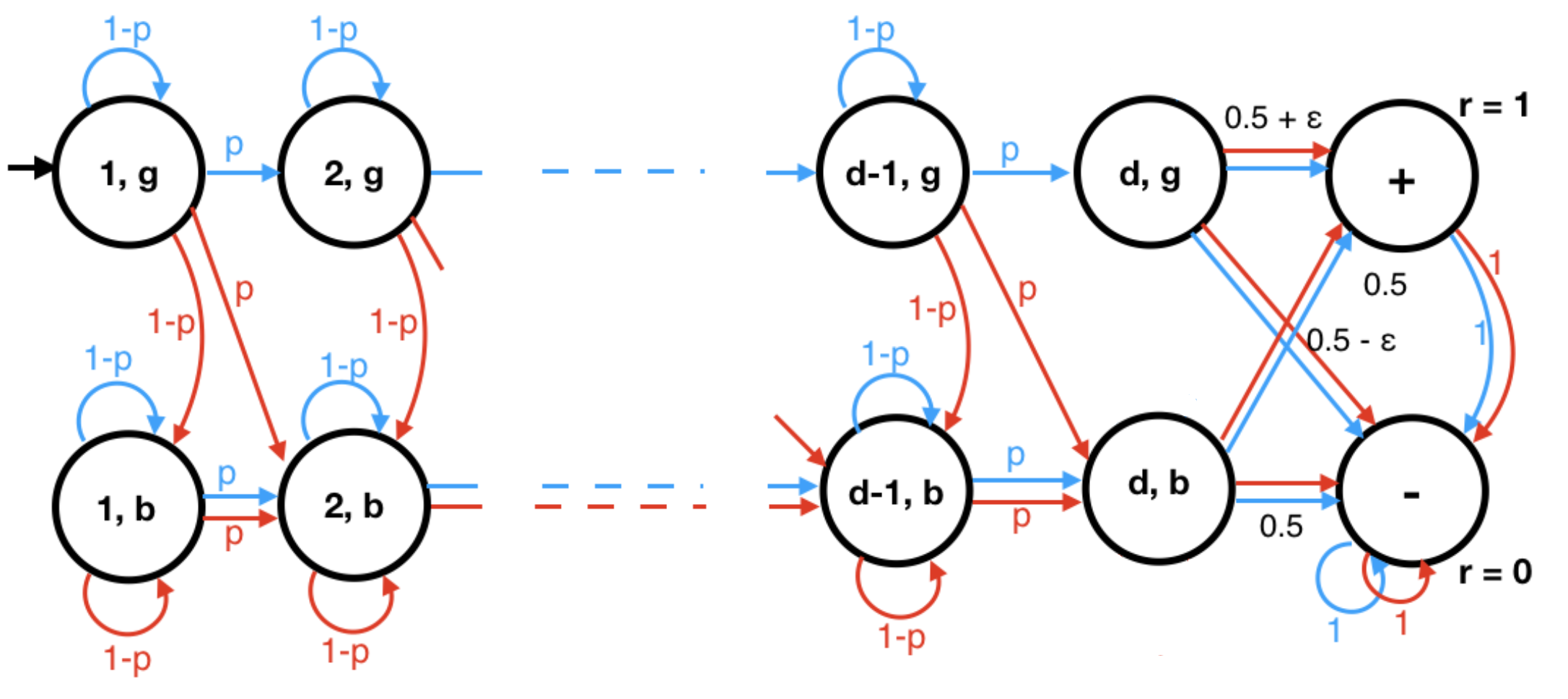
Figure 1: Latent state construction: contextual combination lock. As long as the agent follows actions of $\pi^{*}$(blue arrows), the agent remains in good states $(i,g)$ and receives a Bernoulli($1/2+\varepsilon$) reward but otherwise transits to bad states $(i,b)$ and receives a Bernoulli($1/2$) reward.

6 Adaptive algorithms

In Section 4, the algorithm introduced benefits from the guarantee provided by Theorem 1, which is near optimal in the worst case as the lower bound construction shows. However, in cases where the transition matrix induced by the policy class all have nicer eigenspectra, one could expect to have an improved sample complexity. Ideally, the algorithm should automatically adapt to more favorable eigenspectra. This is precisely what we describe in this section. We give an adaptive algorithm whose sample complexity improves when the eigenspectrum of transition matrices induced by the policy class admits a more favorable property.

6.1 Adaptivitity to the eigenspectrum

Our adaptive algorithm, presented in Algorithm 3 in Appendix D.3, is a policy search algorithm similar to Algorithm 1 where, instead of invoking the procedure ValEstimate, we compute the value function for every policy $\pi$ by invoking the procedure AdaValEstimate given in Appendix D.3.

AdaValEstimate follows along the lines of ValEstimate. When invoked for a policy $\pi$, it first estimates the expected rewards for the first $3d$ time steps. Then, AdaValEstimate computes the auto-regression coefficients $\alpha_{k}(\widehat{\lambda})$, and uses them to predicts the expected rewards for all future time steps by extrapolating. The major difference between ValEstimate and AdaValEstimate is the way the coefficients $\alpha_{k}(\widehat{\lambda})$ are computed. Specifically, using $\Delta\vcentcolon={}2d4^{d}\sqrt{(8K^{3d}\log(6d\left\lvert\Pi\right\rvert)/\delta)/n}$, the procedure AdaValEstimate computes the coefficients $\widehat{\lambda}$ by solving the optimization problem

$$\widehat{\lambda}\leftarrow\operatorname*{argmin}_{\lambda\in\mathbb{C}^{d}} \leavevmode\nobreak\ \prod_{k=2}^{d}\big{(}\sum_{h=0}^{H-1}\lvert\lambda_{k}\rvert^{h}\big{)}\leavevmode\nobreak\ \leavevmode\nobreak\ \leavevmode\nobreak\ \leavevmode\nobreak\ \text{s.t.}\leavevmode\nobreak\ \leavevmode\nobreak\ \lambda_{1}=1,|\lambda_{k}|\leq 1 \textrm{for }2\leq k\leq d,$$

$$\textrm{and }\leavevmode\nobreak\ \Big{\lvert}\sum_{k=1}^{d}(-1)^{k+1}\alpha_{k}(\lambda)\widehat{R}_{h-k}-\widehat{R}_{h}\Big{\rvert}\leq\Delta \textrm{for }d+1\leq h\leq 3d.$$

The above modification to the computation of $\widehat{\lambda}$ allows our error propagation bound to adapt to $\lambda$, which defines the coefficients of autoregression for the expected rewards in policy $\pi$ (given in Lemma 1). The propagated error would be small if the coordinates of $\lambda$ are bounded away from $1$. The policy $\widetilde{\pi}$, returned by Algorithm 3, thus enjoys the following adaptive performance guarantee.

Theorem 3 (Adaptive upper bound).

For a given $\delta\in(0,1)$, $d$-rank MDP, horizon $H$ and a finite policy class $\Pi$, after collecting $n$ episodes, Algorithm 3 returns a policy $\widetilde{\pi}$ that with probability at least $1-\delta$ admits the following guarantee:

$$V^{\widetilde{\pi}} \geq\max_{\pi\in\Pi}V^{\pi}-O\bigg{(}dH^{2}(16e)^{2d}\cdot\max_{\pi^{\prime}\in\Pi}\prod_{k=2}^{d}\Big{(}\sum_{j=0}^{H-1}\lvert\lambda^{\pi^{\prime}}_{k}\rvert^{j}\Big{)}^{2}\sqrt{\frac{K^{3d}\log(6\Pi d/\delta)}{n}}\bigg{)},$$

Proof of Theorem 3 follows along the lines of the proof of Theorem 1 where we replace the error propagation bound (in Lemma 3) by a similar bound that adapts to the eigenspectrum of the transition matrix $T^{\pi}$. We defer the proof details to appendix Appendix D.3. Note that for any $\lvert\lambda_{k}\rvert\leq 1$ and thus $\sum_{h=0}^{H-1}\lvert\lambda_{k}\rvert^{h}\leq H$. Using this fact in Theorem 3 recovers the result of Theorem 1, albeit upto a multiplicative factor of $2^{2d}$. In the following, we provide an example of a low rank MDP problem in which the adaptive bound above could be much better than the worst case upper bound in Theorem 1.

Corollary 1 (Well mixing MDP).

Given $\delta\in(0,1)$, horizon $H$ and a finite policy class $\Pi$. Let $M$ be a $d$-rank MDP such that the second largest eigenvalue of the transition matrix $T^{\pi}$ satisfies $\lvert\lambda^{\pi}_{2}\rvert\leq 1-\gamma\leavevmode\nobreak\$ for every policy $\pi\in\Pi$. Then, after collecting $n$ episodes, our adaptive algorithm returns a policy $\widetilde{\pi}$ that with probability at least $1-\delta$ admits the following guarantee:

$$V^{\widetilde{\pi}}\geq\max_{\pi\in\Pi}V^{\pi}-\widetilde{O}\Big{(}\Big{(}\frac{K}{\gamma}\Big{)}^{2d}\frac{1}{\sqrt{n}}\Big{)},$$

where the $\widetilde{O}$ hides polynomial factors of $d,H,\log(1/\delta)$ and multiplicative constants.

We next show through a lower bound that the adaptive upper bound in Theorem 3 cannot be improved further. We defer the proof details to Appendix E.3.

Theorem 4 (Adaptive lower bound).

Let $\varepsilon\in(0,1/16)$, $\delta\in(0,1/2)$, $d\geq 4$ and $(\lambda_{i})_{i\in[d]}\in[0,1]^{d}$ satisfy

$$d^{2d}\lesssim\prod_{i=1}^{d}\frac{1}{1-\lambda_{i}} \lesssim\exp(H) \sum_{i=1}^{d}\frac{1}{1-\lambda_{i}}\leq\frac{H}{4\ln(4d)}\leavevmode\nobreak\ .$$ and

Then, there is a realizable policy class and a family of MDPs with rank at most $\Theta(d)$, finite observation space, horizon $H$ and two actions such that: For each $i\in[d]$, policy $\pi$ and MDP $M$ in this class, there is an eigenvalue of the induced transition matrix $T^{\pi}_{M}$ in $[\lambda_{i}/2,\lambda_{i}]$. Furthermore, any algorithm that returns, with probability at least $1-\delta$ an $\varepsilon$-optimal policy for any MDP in this family, has to collect at least

$$\Omega\Big{(}\frac{1}{\varepsilon^{2}d^{d}}\sqrt{\prod_{i=1}^{d}\frac{1}{1-\lambda_{i}}}\log\left(1/{2\delta}\right)\Big{)}$$

episodes in expectation in some MDP in this family.

Adaptivity to rank.

In Appendix D.4, we also provide an adaptive algorithm that can find the best policy in the class $\Pi$ without knowing the value of the rank parameter $d^{*}$. Our adaptive algorithm, given in Algorithm 5, follows from standard techniques in the model selection literature. For every $d\in[H]$, we compute an optimal policy $\widetilde{\pi}_{d}$ assuming that the rank $d^{*}=d$. Then, for each $d\in[H]$, we estimate the value function for the policy $\widetilde{\pi}_{d}$ by drawing $n/2H$ fresh trajectories using that policy. Finally, we return the policy $\widetilde{\pi}$ from the set $\left\{\widetilde{\pi}_{d}\right\}_{d\in[H]}$ with the highest estimated value. The returned policy $\widetilde{\pi}$ satisfies, with probability at least $1-\delta$,

$$V^{\widetilde{\pi}}\geq\max_{\pi\in\Pi}\leavevmode\nobreak\ V^{\pi}-\widetilde{O}\Big{(}\Big{(}\frac{H}{d^{*}}\Big{)}^{2d^{*}}\sqrt{\frac{(8K)^{3d^{*}}\log(\left\lvert\Pi\right\rvert/\delta)}{n}}\Big{)}.$$

We defer full details of the analysis to the Appendix.

7 Conclusion

We presented a new analysis of reinforcement learning with rich observations in the agnostic setting, under the low rank MDP assumption. We gave both a non-adaptive and an adaptive algorithm for learning a quasi-optimal policy in this scenario, which we showed to benefit from guarantees that are only polynomial in the horizon and the number of actions, and only logarithmic in the size of the policy class considered. While our bound is exponential in the MDP rank, we give nearly matching lower bounds proving that that dependency is unavoidable. The agnostic setting is a more realistic setting that has received less attention in the literature. We view this work as initiating the study of this general setting under workable assumptions and believe that many other algorithmic and theoretical aspects of such scenarios need to be studied further.

Acknowledgements

Part of the work was performed when AS was an intern at Google Research, NYC. KS acknowledges support from NSF CAREER Award 1750575. YM has received funding from the European Research Council (ERC) under the European Union’s Horizon 2020 research and innovation program (grant agreement No. 882396), by the Israel Science Foundation (grant number 993/17) and the Yandex Initiative for Machine Learning at Tel Aviv University.

Appendix A Detailed comparison to prior work

Provably sample-efficient learning algorithms have been well studied in the classical tabular RL literature (Kearns and Singh, 2002; Brafman and Tennenholtz, 2002). However, the number of samples required by these algorithms to find the optimal policy $\pi^{*}$ scales with the size of the state space $\lvert\mathcal{X}\rvert$ (Jaksch et al., 2010; Lattimore and Hutter, 2012), and thus these methods fail to scale to the rich observation settings where $\lvert\mathcal{X}\rvert$ could be astronomically large. There have been significant recent advances in developing efficient algorithms for such rich observation settings, albeit under additional assumptions. The two main styles of assumptions considered in the literature to make learning tractable are: (a) the learner has access to a value function class $\mathcal{F}$ that realizes the optimal value function $f^{*}$ for the underlying MDP, and (b) the underlying transition dynamics admits additional structure such as low rank or linear decomposition, etc. We note that the goal of these works is to find the optimal policy for the underlying MDP. In comparison, in our work, we assume access to a policy class $\Pi$ and our goal is to find a policy $\widetilde{\pi}$ that could compete with the best policy in the class $\Pi$. In the following, we compare our setup with the assumptions made in the prior work.

RL with general value function approximation.

Recently there has been great interest in designing RL algorithms with general function approximation (Jiang et al., 2017; Dann et al., 2018; Sun et al., 2019; Du et al., 2019a; Wang et al., 2020). In particular, Jiang et al. (2017) introduced the notion of Bellman rank, a measure of complexity that depends on the underlying environment and the value function class $\mathcal{F}$, and provide statistically efficient algorithms for learning problem for which Bellman rank is bounded. This was later extended to model-based algorithms by Sun et al. (2019). While these algorithms work across a variety of problem settings, their sample complexity scales with $\log(\lvert\mathcal{F}\rvert)$. Furthermore, these algorithms also require the optimal value function $f^{*}$ to be realized in $\mathcal{F}$. In our work, we do not assume that the learner has access to a value function class $\mathcal{F}$. In fact, given a value function class $\mathcal{F}$, we can construct the policy class $\Pi_{\mathcal{F}}$ that corresponds to greedy policies induced by the class $\mathcal{F}$. However, given just a policy class $\Pi$, one can not construct a value function class, without additional knowledge of the underlying dynamics.

Example 1.

Let $\mathcal{X}=\left\{0,1,\ldots,N\right\}$, $\mathcal{A}=\{0,1\}$, $\Pi=\{\pi_{0},\pi_{1}\}$ and $H=2$. For every action $a\in\mathcal{A}$, we define the reward $r(x,a)=1$ when $x$ is even, and $r(x,a)=0$ when $x$ is odd. Further, we assume that the transition dynamics $T$ is parameterized by a vector $p\in\left\{0,1\right\}^{N}$ such that for any state $x$, if $p(x)=1$ and $a=1$, then the next state $x^{\prime}$ is sampled uniformly at random from the set of even numbers in $\mathcal{X}$. Otherwise, we sample an odd number uniformly at random for $x^{\prime}$. Clearly, in order to learn the optimal value function, the leaner needs to recover the value of the vector $p$ on at least $O(N)$ states. From standard packing arguments, we get that in $N$ dimensions there are at least $2^{O(N)}$ vectors that are $O(N)$ apart. Thus, any appropriate value function class $\mathcal{F}$ that contains $p$ must have size at least $2^{O(N)}$.

Linear MDP assumption.

Our Assumption 1 implies that for any policy $\pi\in\Pi$, the transition dynamics exhibits a low-rank decomposition with dimension $d$, that is $T^{\pi}(x^{\prime}|x)=\langle\phi^{\pi}(x),\psi^{\pi}(x^{\prime})\rangle,$, for some d-dimensional feature maps $\phi^{\pi},\psi^{\pi}\colon\mathcal{X}\mapsto\mathbb{R}^{d}$. Low rank MDPs and linear transition models have recently gained a lot of attention in the RL literature (Yang and Wang, 2020; Jin et al., 2020b; Modi et al., 2020; Wang et al., 2021b). The works most closely related to our setup are those of Jin et al. (2020b) and Yang and Wang (2020), who give algorithms to find optimal policy in low rank MDPs with known feature maps $\phi$. Similarly, the other algorithms also assume that the learner either observes the feature $\phi(x)$, or the feature $\psi(x)$. However, in our setup, the learner neither observes the features $\phi^{\pi}$ nor the features $\psi^{\pi}$, thus restricting application of these algorithms to our setting.

A new line of work, initiated by Agarwal et al. (2020b), focuses on the representation learning question in the above setting. They assume that the feature functions $\phi$ and $\psi$, although not known to the learner, are realized in the given classes $\Phi$ and $\Psi$ respectively. In order to find the optimal policy, their algorithm first identifies the underlying feature functions $\phi^{*}$ and $\psi^{*}$, and thus, their sample complexity guarantees scale with $\log(\lvert\Phi\rvert\lvert\Psi\rvert)$. Later, Modi et al. (2021) show that a similar approach also works when the learner has only access to a $\Phi$ but not $\Psi$. In comparison, we do not assume knowledge of either classes $\Phi$ or $\Psi$, and instead work with a policy class $\Pi$. In fact, the following simple illustrative example shows that the feature function $\Phi$ could be arbitrarily complex even when $\left\lvert\Pi\right\rvert$ is small, and thus we can not hope to learn the feature function from samples.

Example 2.

Let $\mathcal{X}=[N]$, $\mathcal{A}=\{0,1\}$. We define the feature function $\psi(x)\in\mathbb{R}^{2}$ such that $(1/2N,0)^{\top}$ if $x$ is even and $(0,1/2N)^{\top}$ if $x$ is odd. Further, for $\lambda\geq 0$, define the feature function $\phi_{\lambda}(x)\in\mathbb{R}^{2}$ such that $\phi_{\lambda}(x)=(1,0)^{\top}$ if $\sin(x/\lambda)\geq 0$, and $\phi_{\lambda}(x)=(0,1)^{\top}$ otherwise. In this MDP, the next state $x^{\prime}$ is either sampled uniformly at random from the set of even numbers in $\mathcal{X}$ or sampled uniformly at random from the set of odd numbers in $\mathcal{X}$, depending on the value of $\sin(x/\lambda)$.

Note that the mapping $x\mapsto\sin(x/\lambda)$ could be arbitrarily complex when $\lambda$ is small. In fact, the function class $\Phi=\{\lambda\mid x\mapsto\sin(x/\lambda)\}$ has infinite VC dimension. Thus, one cannot hope to learn the feature function $\phi_{\lambda}$ from samples.

It is worth noting that in the above example, FLAMBE (Agarwal et al., 2020b), MOFFLE (Modi et al., 2021), or in fact any other approach that attempts to recover the feature function $\phi$, as mentioned above will not succeed. Furthermore, when $\lvert\Pi\rvert$ is large and the length of the episode $H$ is large, the previously known agnostic upper bounds of $\tfrac{\lvert\Pi\rvert}{\varepsilon^{2}}$ or $\tfrac{2^{H}\log(\lvert\Pi\rvert)}{\varepsilon^{2}}$ are also prohibitively large. However, in the above example, our algorithm enjoys a sample complexity bound of ${\tfrac{H^{4}\log(\lvert\Pi\rvert)}{\varepsilon^{2}}}$.

Finally, note that in our setup, the decomposition of the induced transition kernel (into $\phi^{\pi}$ and $\psi^{\pi}$) may be different for each policy $\pi$ in the class $\Pi$. Furthermore, there may be policies outside of $\Pi$ that do not even exhibit such a low-rank decomposition. Thus, although our low rank assumption is similar to those in linear or low-rank MDPs (Agarwal et al., 2020b), our model is more general.

Comparison to Block MDP model.

Krishnamurthy et al. (2016) introduced the block MDP model, where a small number of latent states $\mathcal{S}$ govern the transition dynamics, and the observations $x\in\mathcal{X}$ are generated depending on the current latent state $s$. In this model, there is a decoding function $g^{*}$ that maps observations $x$ back to the latent state $s$ that generates $x$. Du et al. (2019a); Misra et al. (2020) assume that the learner is given a realizable class of decoding functions $\mathcal{G}$ and show that the true mapping $g^{*}\in\mathcal{G}$ can be learnt efficiently, both computationally and statistically, which can then be used to find the optimal policy. However, note that the transition matrix in a Block MDPs with $S$ latent states has rank at most $\lvert S\rvert$, and thus their model is captured by our Assumption 1. However, in our setup, we do not assume that the leaner has access to the class $\mathcal{G}$. In fact, Example 2 above shows that the latent state map $g^{*}$ (the mapping $\phi_{\lambda}(x)$ in that case) could be arbitrarily complex even when $\Pi$ is small, and thus we can not hope to learn $g^{*}$ from samples.

Policy gradient methods.

Model free direct policy search algorithms that directly maximize the value function have shown tremendous empirical success (Kakade, 2001; Kakade and Langford, 2002; Levine and Koltun, 2013; Schulman et al., 2015, 2017), and recently, have been analysed from a theoretical perspective (Agarwal et al., 2021; Abbasi-Yadkori et al., 2019; Bhandari and Russo, 2019; Liu et al., 2020; Agarwal et al., 2020a). While these methods operate directly on a policy class $\Pi$, as we do in our work, they require additional modelling assumptions in order to succeed; foremost being that the policy class $\Pi$ exhibits a differentiable paraeterization. Further assumptions include that the policy class $\Pi$ contains the optimal policy $\pi^{*}$, the policy class $\Pi$ has a good coverage over the state space (Agarwal et al., 2021), and that the underling MDP has a linear factorization with known feature maps (Agarwal et al., 2020a). We do not require these assumptions.

DICE/DualDICE algorithms.

Recent works of Liu et al. (2018) and Nachum et al. (2019) provide estimators that do not suffer the curse of horizon, i.e. the factor of $A^{H}$, in off-policy estimation of expected policy rewards by applying importance sampling on average visitation distributions of single steps of state-action pairs, instead of the much higher dimensional distribution of the whole trajectories. However, their estimator requires access to a function class $\mathcal{H}$ that contains the importance weights of the average visitation distribution. We do not require access to such a class $\mathcal{H}$ in our estimator of expected policy rewards.

POMDP with reactive policies.

We will show in the following that our theory and algorithm applies to partially observable Markov decision processes (POMDPs), as long as policies are reactive, that is, only take the current observation into account. Although existing works such as (Jiang et al., 2017) show polynomial sample-complexity bounds for POMDPs with reactive policy classes, they require the optimal policy to be reactive, which is not true in POMDPs in general. In contrast, we can handle the important scenario where reactive policies can achieve good but not necessarily close to optimal performance and we are interested in finding the best such policy.

A POMDP consists of a MDP with finite state space $\mathcal{S}$, action space $\mathcal{A}$ and horizon $H$ where observed rewards at each step are drawn from a distribution with mean $r(s_{h},a_{h})$ that depends on the current state $s_{h}$ and action $a_{h}$. Similarly, the next state is drawn fron a transition kernel $P(s_{h+1}|s_{h},a_{h})$. However, in a POMDP, the current state is not observable and the agent instead receives an observation $x_{h}\in\mathcal{X}$. We consider the formulation where the observation is drawn from a distribution $O(x_{h}|s_{h})$ that depends on the current latent state $s_{h}$. Unlike in, e.g., Block MDP models, $x_{h}$ does not need to be sufficient to decode $s_{h}$ and this model does not need to be an MDP over the observation space $\mathcal{X}$. As a consequence, the optimal actions do in general depend on all previous observations. Nonetheless, reactive policies which are of the form $\mathcal{X}\rightarrow\mathcal{A}$ and only take the current observation into account, often achieve good performance and are of particular interest in practice due to their simplicity.

Since a POMDP may not be a MDP over observations, such models are formally outside of our scope. However, as our technique never explicitly accesses observations except through the policy, we can cast a POMDP problem as follows in our framework. For any policy $\pi\colon\mathcal{X}\rightarrow\mathcal{A}$ in our policy class $\Pi$ we define a stochastic policy $\pi^{\prime}$ over latent states as $\pi^{\prime}(a|s)=\sum_{x\in\mathcal{X}}\mathbbm{1}\left\{\pi(x)=a\right\}O(x|s)$ and denote the class of these policies by $\Pi^{\prime}\subseteq\mathcal{S}\rightarrow\Delta(\mathcal{A})$. Running our algorithms on a POMDP with policy class $\Pi$ is equivalent to running them on an MDP with direct access to latent states $\mathcal{S}$ and policy class $\Pi^{\prime}$. Since an MDP with finite state space $\mathcal{S}$ has rank at most $|\mathcal{S}|$, our guarantees apply to POMDPs with a reactive policy class and we can set $d=|\mathcal{S}|$.

Exponential lower bounds for planning and offline RL.

Several publications (Wang et al., 2021a; Zanette, 2020; Weisz et al., 2021) recently provide exponential lower bounds for learning the optimal policy with access to a realizable linear Q-function class $\mathcal{F}$ of dimension $d$ in several settings. Most related is Wang et al. (2021a), wo study offline RL where the agent has only access to a dataset of transition samples and show even if the dataset has good coverage of the features of $\mathcal{F}$, a sample complexity that is exponential in $d$ or $H$ is unavoidable. In contrast, we allow the agent to collect samples arbitrarily by interacting with the MDP and although our algorithms first collect a dataset non-adaptively, the uniform action choices ensure good state coverage as opposed to just feature coverage which avoids the existing lower bounds.

Appendix B Cayley-Hamilton theorems

The following result holds for any matrix $A$ with rank $d$.

Lemma 4 (Cayley-Hamilton Theorem for rank $d$ matrices (Segercrantz, 1992)).

Let $A\in\mathbb{C}^{N\times N}$ be a matrix with rank at most $d$, where $d\leq N$, and let $\lambda=\left(\lambda_{1},\ldots,\lambda_{d}\right)\in\mathbb{C}^{d}$ denote the set of eigenvalues of $A$. Then, $A$ satisfies the relation

$$A^{d+1} =\sum_{k=1}^{d}(-1)^{k+1}\alpha_{k}(\lambda)A^{d+1-k},$$

where the coefficient $\alpha_{k}(\lambda)$ are given by the sum of degree $k$ monomials:

$$\alpha_{k}(\lambda)=\sum_{x\in\{0,1\}^{d}\text{\leavevmode\nobreak\ s.t.\leavevmode\nobreak\ }\|x\|_{1}=k}\lambda_{1}^{x_{1}}\lambda_{2}^{x_{2}}\ldots\lambda_{d}^{x_{d}}.$$

The proof of the above follows from the characteristic polynomial for rank $d$ matrices, which allows us to express $d+1$-th power for any matrix $A$ in terms of the lower powers.

We will soon provide an extension of the above result which allows us to express the $n$-th power of the matrix $A$ in terms of the lower powers. Before doing so, we need to define some additional notation.

B.1 Coefficients $\alpha_{m,k}$

For any $m\geq 0$ and $k\geq 0$, we first define the coefficients $\alpha_{m,k}$.

Definition 1.

For any $k\geq 0$ and $\lambda=(\lambda_{1},\ldots,\lambda_{d})\in\mathbb{C}^{d}$, define $\alpha_{m,k}(\lambda)$ to denote the quantity

$$\alpha_{m,k}(\lambda)\vcentcolon={}\sum_{y\in\left\{0,\ldots,m\right\}^{d}}\mathbbm{1}\Big{\{}\sum_{j=1}^{d}\mathbbm{1}\left\{y_{j}>0\right\}=k\leavevmode\nobreak\ {\text{and}}\leavevmode\nobreak\ \sum_{j=1}^{d}y_{j}=m\Big{\}}\prod_{j=1}^{d}\lambda_{j}^{y_{j}}.$$ (7)

whenever $m\geq k$ and $\alpha_{m,k}=0$ when $m\leq k$ or $k>d$. Further, for the ease of notation, for any $k\in[d]$, we define $\alpha_{k}(\lambda)$ to denote the quantity $\alpha_{k,k}(\lambda)$.

The following lemma provides a useful technical relation between the coefficients $\alpha_{m,k}$ defined above.

Lemma 5.

For any $m\geq 0$, $k\in[d]$ and $\lambda\in\mathbb{C}^{d}$, the quantities $(\alpha_{m,k})_{k\in[d],m\geq 0}$ given in Definition 1 satisfy

$$\sum_{j=1}^{m\wedge d}\alpha_{m,j}(\lambda)\cdot\alpha_{k,k}(\lambda) =\sum_{j^{\prime}=k+1}^{(m+k)\wedge d}{j^{\prime}\choose k}\alpha_{m+k,j^{\prime}}(\lambda).$$

Proof.

For the sake of the proof, we will be interpreting $\alpha_{m,j}(\lambda)$ and $\alpha_{k,k}(\lambda)$ as symmetric polynomials with $\lambda$ as the formal variables. The value of these quantities can be computed by plugging in the value of $\lambda_{1},\ldots,\lambda_{d}$ for $\lambda$.

Thus, $\alpha_{m,j}$ denotes a symmetric sum of monomials, where each monomial term has $j$ variables with sum of all the powers in that monomial being $m$. Similarly, $\alpha_{k,k}$ denotes a symmetric sum of monomials, where each monomial term has $k$ variables each with the power of $1$. Subsequently, when we take the product $\alpha_{m,j}\cdot\alpha_{k,k}$, we will get monomial terms, where in each term the sum of all the powers is $m+k$, but the total number of distinct variables can range from $k+1$ to $\min\left\{j+k,d\right\}$. Since, the polynomials $\alpha_{m,j}$ and $\alpha_{k,k}$ are symmetric in $\lambda$, the resultant polynomial that we will get after taking their product will also be symmetric. Furthermore, each of the monomial terms with $j^{\prime}$ distinct variables can be generated through ${j^{\prime}\choose k}$ different splits with $k$ variables that go into $\alpha_{k,k}(\lambda)$ and the rest $j^{\prime}-k$ variables that go into $\alpha_{m,j^{\prime}-k}(\lambda)$. Hence, the coefficient of $\alpha_{m+k,j^{\prime}}$ would be exactly ${j^{\prime}\choose k}$. We formalize this in the following:

$$\sum_{j=1}^{m\wedge d}\alpha_{m,j}(\lambda)\cdot\alpha_{k,k}(\lambda) =\sum_{j=1}^{m\wedge d}\Bigg{(}\sum_{y\geq 0}\mathbbm{1}\Big{\{}\sum_{i=1}^{d}\mathbbm{1}\left\{y_{i}>0\right\}=j\text{\leavevmode\nobreak\ and\leavevmode\nobreak\ }\sum_{i=1}^{d}y_{i}=m\Big{\}}\prod_{i=1}^{d}\lambda_{i}^{y_{i}}\leavevmode\nobreak\ \times$$

$$\qquad\qquad\qquad\qquad\sum_{y^{\prime}\geq 0}\mathbbm{1}\Big{\{}\sum_{i=1}^{d}\mathbbm{1}\left\{y^{\prime}_{i}>0\right\}=k\text{\leavevmode\nobreak\ and\leavevmode\nobreak\ }\sum_{i=1}^{d}y^{\prime}_{i}=k\Big{\}}\prod_{i=1}^{d}\lambda_{i}^{y^{\prime}_{i}}\Bigg{)}$$

$$=\sum_{j=1}^{m\wedge d}\sum_{\begin{subarray}{c}y,y^{\prime}\geq 0\end{subarray}}\mathbbm{1}\Big{\{}\sum_{i=1}^{d}\mathbbm{1}\left\{y_{i}>0\right\}=j\wedge\sum_{i=1}^{d}\mathbbm{1}\left\{y^{\prime}_{i}>0\right\}=k\wedge\sum_{i=1}^{d}y_{i}=m\wedge\sum_{i=1}^{d}y^{\prime}_{i}=k\Big{\}}\prod_{i=1}^{d}\lambda_{i}^{y_{i}+y^{\prime}_{i}}$$

$$=\sum_{j^{\prime}=k+1}^{(m+k)\wedge d}{j^{\prime}\choose k}\sum_{y,y^{\prime}\geq 0}\mathbbm{1}\Big{\{}\sum_{i=1}^{d}\mathbbm{1}\left\{y_{i}+y^{\prime}_{i}>0\right\}=j^{\prime}\text{\leavevmode\nobreak\ and\leavevmode\nobreak\ }\sum_{i=1}^{d}y_{i}+y^{\prime}_{i}=m+k\Big{\}}\prod_{i=1}^{d}\lambda_{i}^{y_{i}+y^{\prime}_{i}}$$

$$=\sum_{j^{\prime}=k+1}^{(m+k)\wedge d}{j^{\prime}\choose k}\sum_{y^{\prime\prime}\geq 0}\mathbbm{1}\Big{\{}\sum_{i=1}^{d}\mathbbm{1}\left\{y^{\prime\prime}_{i}>0\right\}=j^{\prime}\text{\leavevmode\nobreak\ and\leavevmode\nobreak\ }\sum_{i=1}^{d}y^{\prime\prime}_{i}=m+k\Big{\}}\prod_{i=1}^{d}\lambda_{i}^{y^{\prime\prime}_{i}}$$

$$=\sum_{j^{\prime}=k+1}^{(m+k)\wedge d}{j^{\prime}\choose k}\cdot\alpha_{m+k,j^{\prime}},$$

where $y^{\prime\prime}_{i}\vcentcolon={}y_{i}+y^{\prime}_{i}$ and the third equality in the above follows by rearranging the terms while satisfying the constraints inside the indicator. ∎

We next provide a bound on the value of $\alpha_{m,k}$ as a function of $m$ and $k$.

Lemma 6.

For any $d\geq 1$, $m\geq 0$, $k\leq\min\left\{d,m\right\}$ and $\lambda\in\mathbb{C}^{d}$, that satisfies $\left\lvert\lambda_{j}\right\rvert\leq 1$ for all $j\in[d]$, the quantities $\alpha_{m,k}(\lambda)$ given in Definition 1 satisfy the bound

$$\left\lvert\alpha_{m,k}(\lambda)\right\rvert\leq\Big{(}\frac{4e\max\{m,d\}}{d}\Big{)}^{d}.$$

Furthermore, for $k=m\leq d$, we have that $\alpha_{k}(\lambda)=\alpha_{k,k}(\lambda)\leq{4}^{d}$.

Proof.

Starting from the definition of $\alpha_{m,k}(\lambda)$, we note that

$$\left\lvert\alpha_{m,k}(\lambda)\right\rvert =\Big{\lvert}\sum_{y\in\left\{0,\ldots,m\right\}^{d}}\mathbbm{1}\Big{\{}\sum_{j=1}^{d}\mathbbm{1}\left\{y_{j}>0\right\}=k\leavevmode\nobreak\ {\text{and}}\leavevmode\nobreak\ \sum_{j=1}^{d}y_{j}=m\Big{\}}\prod_{j=1}^{d}\lambda_{j}^{y_{j}}\Big{\rvert}$$

$$\leq\sum_{y\in\left\{0,\ldots,m\right\}^{d}}\mathbbm{1}\Big{\{}\sum_{j=1}^{d}\mathbbm{1}\left\{y_{j}>0\right\}=k\leavevmode\nobreak\ {\text{and}}\leavevmode\nobreak\ \sum_{j=1}^{d}y_{j}=m\Big{\}}\Big{\lvert}\prod_{j=1}^{d}\lambda_{j}^{y_{j}}\Big{\rvert}$$

$$=\sum_{y\in\left\{0,\ldots,m\right\}^{d}}\mathbbm{1}\Big{\{}\sum_{j=1}^{d}\mathbbm{1}\left\{y_{j}>0\right\}=k\leavevmode\nobreak\ {\text{and}}\leavevmode\nobreak\ \sum_{j=1}^{d}y_{j}=m\Big{\}}\prod_{j=1}^{d}\left\lvert\lambda_{j}^{y_{j}}\right\rvert$$

$$\leq\sum_{y\in\left\{0,\ldots,m\right\}^{d}}\mathbbm{1}\Big{\{}\sum_{j=1}^{d}\mathbbm{1}\left\{y_{j}>0\right\}=k\leavevmode\nobreak\ {\text{and}}\leavevmode\nobreak\ \sum_{j=1}^{d}y_{j}=m\Big{\}},$$

where the inequality in the second line follows from an application of Triangle inequality. The last line holds because $|\lambda_{j}|\leq 1$, and thus $|\prod\lambda_{j}^{y_{j}}|\leq 1$ for any $y$. We note that the right hand side in the above expression denotes the number of ways of distributing $m$ balls into $d$ bins such that exactly $k$ of them are non-empty. If $m=k=1$, we get that $\left\lvert\alpha_{m,k}(\lambda)\right\rvert\leq 1$. Otherwise, a simple counting argument implies that

$$\left\lvert\alpha_{m,k}(\lambda)\right\rvert \leq{d\choose k}{m-1\choose k-1}\leq 2^{d}\cdot{m-1\choose k-1}.$$

When $m\leq d$ or $k=1$, we can simply upper bound the above as

$$\left\lvert\alpha_{m,k}(\lambda)\right\rvert\leq 2^{d}\cdot 2^{m}\leq 4^{d}.$$

Next, when $m>d$ and $k\geq 2$, using the fact that ${N\choose n}\leq\left(eN/n\right)^{n}$ for any $0<n\leq N$, we get that

$$\left\lvert\alpha_{m,k}(\lambda)\right\rvert \leq 2^{d}\cdot\left(\frac{e(m-1)}{(k-1)}\right)^{k}$$

$$\leq 2^{d}\cdot\left(\frac{2em}{k}\right)^{k}$$

$$\leq 2^{d}\cdot\left(\frac{2em}{d}\right)^{d},$$

where the inequality in the second line above holds because $(m-1)/(k-1)\leq 2m/k$ for $k\geq 2$, and the inequality in the last line holds because the function $\left(x/y\right)^{y}$ is an increasing function of $y$ when $x\geq ey$.

Considering the above two bounds together implies that:

$$\left\lvert\alpha_{m,k}(\lambda)\right\rvert \leq\Big{(}\frac{4e\max\{m,d\}}{d}\Big{)}^{d}.$$

∎

B.2 Coefficients $\beta_{m,k}$

We next define the coefficients $\beta_{m,k}$ which will be useful in our upper bound analysis.

Definition 2.

For any $d\geq 1$, $\lambda\in\mathbb{C}^{d}$ and $m\geq 0$, define the vector $\beta_{m}(\lambda)\in\mathbb{C}^{d}$ using the following recursion:

1. $\beta_{0}(\lambda)\vcentcolon={}(\alpha_{1}(\lambda),\ldots,\alpha_{d}(\lambda))^{\top}$, and,

2. For $m\geq 1$, define $\beta_{m}(\lambda)\vcentcolon={}\left(\beta_{m,1}(\lambda),\ldots,\beta_{m,d}(\lambda)\right)^{\top}$ as

   $$\beta_{m,k}(\lambda) =\begin{cases}\beta_{m-1,1}(\lambda)\cdot\alpha_{k}(\lambda)-\beta_{m-1,k+1}(\lambda)&\text{for}\leavevmode\nobreak\ 1\leq k\leq d-1\\ \beta_{m-1,d}(\lambda)\cdot\alpha_{d}(\lambda)&\text{for}\leavevmode\nobreak\ {k=d}\end{cases},$$

where $\alpha_{k}(\lambda)$ is as defined in (7) , and $\beta_{0,k}$ denotes the $k$-th coordinate of the vector $\beta_{0}$.

The next technical lemma provides a relation between the $\beta$ and $\alpha$ values defined above.

Lemma 7.

For any $m\geq 0$ and $k\in[d]$,

$$\beta_{m,k}(\lambda)=\sum_{j=k}^{(m+k)\wedge d}{j-1\choose k-1}\alpha_{m+k,j}(\lambda).$$ (8)

Proof.

We prove the desired relation via induction over $m$. For the base case, when $m=0$, from the definition of $\beta_{0,k}$, we note that

$$\beta_{0,k} =\alpha_{k,k}(\lambda)=\sum_{j=k}^{k}{k-1\choose k-1}\alpha_{k,j}(\lambda).$$

Now, we proceed to the induction step. Assume that the relation (8) holds for all $m^{\prime}<m$. Thus, for any $k\in[d]$, from the definition of $\beta_{m,k}(\lambda)$, we have that

$$\beta_{m,k}(\lambda) =\beta_{m-1,1}(\lambda)\cdot\beta_{0,k}(\lambda)-\beta_{m-1,k+1}(\lambda)$$

$$=\Big{(}\sum_{j=1}^{m\wedge d}\alpha_{m,j}(\lambda)\Big{)}\cdot\alpha_{k,k}(\lambda)-\sum_{j=k+1}^{(m+k)\wedge d}{j-1\choose k}\cdot\alpha_{m+k,j}(\lambda),$$

where the equality in the second line follows from using the relation (8) for time step $m-1$. Using the identity in Lemma 5 in the above, we get that

$$\beta_{m,k}(\lambda) =\sum_{j=k}^{(m+k)\wedge d}{j\choose k}\cdot\alpha_{m+k,j}(\lambda)-\sum_{j=k+1}^{(m+k)\wedge d}{j-1\choose k}\cdot\alpha_{m+k,j}(\lambda)$$

$$=\sum_{j=k}^{(m+k)\wedge d}{j-1\choose k-1}\cdot\alpha_{m+k,j}(\lambda),$$

where the last line uses the relation ${j\choose k}={j-1\choose k-1}+{j-1\choose k}$. This completes the induction step. Thus, proving that the relation (8) holds for all $m\geq 0$ and $k\in[d]$. ∎

We next provide a bound on the value of the coefficients $\beta_{m,k}$ as a function of $m$ and $k$.

Lemma 8.

For any $d\geq 1$, $m\geq 0$, $k\leq d$ and $\lambda\in\mathbb{C}^{d}$, such that $\left\lvert\lambda_{j}\right\rvert\leq 1$ for all $j\in[d]$, the quantities $\beta_{m,k}(\lambda)$ defined in Definition 2 satisfy the bound

$$\lvert\beta_{m,k}(\lambda)\rvert\leq\Big{(}\frac{8e\max\{m+k,d\}}{d}\Big{)}^{d}.$$

Proof.

As a consequence of Lemma 7, we have that for any $m\geq 0$ and $k\in[d]$,

$$\beta_{m,k}(\lambda)=\sum_{j=k}^{(m+k)\wedge d}{j-1\choose k-1}\cdot\alpha_{m+k,j}(\lambda).$$

Thus, using Triangle inequality, we have that

$$\lvert\beta_{m,k}\rvert =\Big{\lvert}\sum_{j=k}^{(m+k)\wedge d}{j-1\choose k-1}\cdot\alpha_{m+k,j}(\lambda)\Big{\rvert}$$

$$\leq\sum_{j=k}^{(m+k)\wedge d}{j-1\choose k-1}\cdot\lvert\alpha_{m+k,j}(\lambda)\rvert.$$

Plugging in the bound on $\lvert\alpha_{m+k,j}(\lambda)\rvert$ from Lemma 6 in the above, we get that

$$\lvert\beta_{m,k}\rvert \leq\sum_{j=k}^{d}{j-1\choose k-1}\cdot\Big{(}\frac{4e\max\{m+k,d\}}{d}\Big{)}^{d}$$

$$\overset{\left(i\right)}{\leq{}}{d\choose k}\cdot\Big{(}\frac{4e\max\{m+k,d\}}{d}\Big{)}^{d}$$

$$\overset{\left(ii\right)}{\leq{}}\Big{(}\frac{8e\max\{m+k,d\}}{d}\Big{)}^{d},$$

where the inequality in $\left(i\right)$ is given by the fact that any $N$ and $n$, we have $\sum_{j=n}^{N}{j\choose n}={N+1\choose n+1}$, and the inequality in $\left(ii\right)$ holds because for any $k\leq d$, ${d\choose k}\leq 2^{d}$. ∎

B.3 Extension of the Cayley-Hamilton theorem

The following result is an extension of the Cayley-Hamilton theorem (Lemma 4) for rank $d$ matrices, and relies on the coefficients $\beta_{m,k}$ defined above.

Lemma 9 (Cayley-Hamilton Theorem extension).

Let $A\in\mathbb{C}^{N\times N}$ be a matrix with rank at most $d$, where $d\leq N$, and let $\lambda=\left(\lambda_{1},\ldots,\lambda_{d}\right)\in\mathbb{C}^{d}$ denote the set of eigenvalues of $A$. Then, for any $m\geq 0$,

$$A^{d+m+1} =\sum_{k=1}^{d}(-1)^{k+1}\beta_{m,k}(\lambda)A^{d+1-k}$$ (9)

where the coefficients vector $\beta_{m}(\lambda)\vcentcolon={}\left(\beta_{m,1}(\lambda),\ldots,\beta_{m,k}(\lambda)\right)$ are given in Definition 2.

Proof.

We give a proof by induction over $m$. For the base case, when $m=0$, Lemma 4 implies that

$$A^{d+1} =\sum_{k=1}^{d}(-1)^{k+1}\alpha_{k}(\lambda)A^{d+1-k}=\sum_{k=1}^{d}(-1)^{k+1}\beta_{0,k}(\lambda)A^{d+1-k},$$ (10)

where the second equality follows form the definition of the vector $\beta_{0}(\lambda)$. We next prove the induction step.

Assume that the relation (9) holds for all $m^{\prime}<m$. We note that

$$A^{d+1+m} =AA^{d+1+(m-1)}$$

$$\overset{\left(i\right)}{=}A\Big{(}\sum_{k=1}^{d}(-1)^{k+1}\beta_{m-1,k}(\lambda)\cdot A^{d+1-k}\Big{)}$$

$$=\beta_{m-1,1}(\lambda)A^{d+1}+\sum_{k=2}^{n}(-1)^{k+1}\beta_{m-1,k}(\lambda)\cdot A^{d+2-k}$$

$$=\beta_{m-1,1}(\lambda)A^{d+1}+\sum_{k=1}^{n-1}(-1)^{k}\beta_{m-1,k+1}(\lambda)\cdot A^{d+1-k}.$$

where the equality in $\left(i\right)$ following from using the relation (9) for time step $m-1$. Plugging in the expansion for $A^{d+1}$ from (10) in the above, we get that

$$A^{d+1+m} =\beta_{m-1,1}(\lambda)\Big{(}\sum_{k=1}^{d}(-1)^{k+1}\beta_{0,k}(\lambda)\cdot A^{d+1-k}\Big{)}+\sum_{k=1}^{d-1}(-1)^{k}\beta_{m-1,k+1}(\lambda)\cdot A^{d+1-k}$$

$$=\sum_{k=1}^{d}(-1)^{k+1}\left(\beta_{m-1,1}(\lambda)\cdot\beta_{0,k}(\lambda)-\beta_{m-1,k+1}(\lambda)\right)A^{d+1-k}.$$ (11)

where in the second line, we defined $\beta_{m-1,d+1}=0$. We next note that for any $k\in[d]$,

$$\beta_{m-1,1}(\lambda)\cdot\beta_{0,k}(\lambda)-\beta_{m-1,k+1}(\lambda) =\beta_{m-1,1}(\lambda)\cdot\alpha_{k}(\lambda)-\beta_{m-1,k+1}(\lambda)$$

$$=\beta_{m,k}(\lambda),$$

where the second line above follows from the definition of $\beta_{m,k}$. Using this relation in (10), we get that

$$A^{d+1+m} =\sum_{k=1}^{d}(-1)^{k+1}\beta_{m,k}(\lambda)A^{d+1-k},$$

hence completing the induction step. Thus, the relation (9) holds for all $m\geq 0$. ∎

Appendix C Missing proofs from Section 4

C.1 Proof of Lemma 1

See 1

Proof.

For any time step $h\geq 1$, let $\mu^{\pi}_{h}$ denote the distribution over the observation space $\mathcal{X}$ at time step $h$ when starting from the initial distribution $\mu_{0}$ and taking actions according to the policy $\pi$. Using the definition of the transition matrix $T^{\pi}$, we note that

$$\mu^{\pi}_{h}=T^{\pi}\mu^{\pi}_{h-1},$$ (12)

where $\mu^{\pi}_{0}$ is defined as $\mu_{0}$. Further, let $\nu^{\pi}\in\mathbb{R}^{\mathcal{X}}$ denotes the vector of expected rewards under policy $\pi$ on the observation space, i.e., for any observation $x\in\mathcal{X}$,

$$\nu^{\pi}(x)\vcentcolon={}\operatorname{\mathbb{E}}_{a\sim\pi(x)}\left[r(s,a)\right].$$

Thus, for any $h\leq H$, the expected reward $R^{\pi}_{h}$ is given by the expression

$$R^{\pi}_{h} =\langle\nu^{\pi},\mu_{h}^{\pi}\rangle=\langle\nu^{\pi},(T^{\pi})^{d+1}\mu_{h-d-1}^{\pi}\rangle,$$ (13)

where the second equality follows from recursively using the relation (12). Using the Cayley-Hamilton theorem (Lemma 4) for the matrix $T^{\pi}$, with rank at most $d$, we get that

$$(T^{\pi})^{d+1} =\sum_{k=1}^{d}(-1)^{k+1}\alpha_{k}(\lambda)(T^{\pi})^{d+1-k},$$

where $\lambda=\left(\lambda^{\pi}_{1},\ldots,\lambda^{\pi}_{d}\right)$ denotes the set of eigenvalues of $T^{\pi}$. Plugging the above in relation (13) for $h\geq d+1$, we get that

$$R^{\pi}_{h} =\langle\nu^{\pi},{\sum_{k=1}^{d}\alpha_{k}(\lambda)(T^{\pi})^{d+1-k}}\mu_{h-d-1}^{\pi}\rangle$$

$$=\sum_{k=1}^{d}(-1)^{k+1}\alpha_{k}(\lambda)\langle\nu^{\pi},\mu_{h-k}^{\pi}\rangle=\sum_{k=1}^{d}(-1)^{k+1}\alpha_{k}(\lambda)R^{\pi}_{h-k},$$

where the last equality follows from plugging back the expression for $R^{\pi}_{h-k}$ from (13). ∎

C.2 Proof of Lemma 2

The following result provides an upper bound on the error in our estimates for the expected reward for any policy $\pi\in\Pi$.

See 2

Proof.

First fix any $h\in[3d]$ and $\pi\in\Pi$. The expected policy reward estimate is given by

$$\widehat{R}^{\pi}_{h} =\frac{1}{n}\sum_{i=1}^{n}r_{h}^{t}\prod_{h^{\prime}\leq h}\left(K\mathbbm{1}\left\{\pi(x^{t}_{h^{\prime}})=a_{h^{\prime}}^{t}\right\}\right)$$

Clearly, $\widehat{R}^{\pi}_{h}$ is an unbiased estimate of $R^{\pi}_{h}$ as

$$\mathbb{E}^{\bar{\pi}}[\widehat{R}^{\pi}_{h}] =\frac{1}{n}\sum_{t=1}^{n}\operatorname{\mathbb{E}}^{\bar{\pi}}\Big{[}r_{h}^{t}\prod_{h^{\prime}\leq h}\left(K\mathbbm{1}\left\{\pi(x^{t}_{h^{\prime}})=a_{h^{\prime}}^{t}\right\}\right)\Big{]}$$

$$=\frac{1}{n}\sum_{t=1}^{n}\mathbb{E}^{\bar{\pi}}\Big{[}r_{h}^{t}\prod_{h^{\prime}\leq h}\frac{\pi(a^{t}_{h^{\prime}}|x^{t}_{h^{\prime}})}{\bar{\pi}(a^{t}_{h^{\prime}}|x^{t}_{h^{\prime}})}\Big{]}$$

$$=\frac{1}{n}\sum_{t=1}^{n}\mathbb{E}^{\pi}[r_{h}^{t}]=\frac{1}{n}\sum_{t=1}^{n}R^{\pi}_{h}=R^{\pi}_{h},$$

where $\bar{\pi}$ denotes the stochastic policy that picks actions uniformly at random and is used to draw the trajectory $(x_{h}^{t},a_{h}^{t},r_{h}^{t})_{h=1}^{H}$ for $t\in[n]$. The equality in the second line above follows from the definition of $\bar{\pi}$ and the last line follows by a change of measure to the case where the trajectories are sampled using the policy $\pi$. We next consider the second moment of each individual term in the estimator

$$\mathbb{E}^{\bar{\pi}}\Big{[}(r_{h}^{t})^{2}\prod_{h^{\prime}\leq h}\left(K\mathbbm{1}\left\{\pi(x^{t}_{h^{\prime}})=a_{h^{\prime}}^{t}\right\}\right)^{2}\Big{]} \overset{\left(i\right)}{\leq}K^{2h}\prod_{h^{\prime}\leq h}\mathbb{P}^{\bar{\pi}}\left(\pi(x^{t}_{h^{\prime}})=a^{t}_{h^{\prime}}\right)$$

$$\overset{\left(ii\right)}{=}K^{2h}\cdot\frac{1}{K^{h}}=K^{h},$$

where the inequality $\left(i\right)$ uses that $0\leq r^{i}_{h}\leq 1$, and the inequality $\left(ii\right)$ holds because $\bar{\pi}$ draws actions uniformly at random which implies that $\mathbb{P}^{\bar{\pi}}\left(a^{i}_{h^{\prime}}=\pi(x^{i}_{h^{\prime}})\mid x^{i}_{h^{\prime}}\right)=1/K$. Therefore the variance for the $t$th sample,

$$\mathbb{V}^{\bar{\pi}}\Big{[}r_{h}^{t}\prod_{h^{\prime}\leq h}\left(K\mathbbm{1}\left\{\pi(x^{t}_{h^{\prime}})=a_{h^{\prime}}^{t}\right\}\right)\Big{]}\leq K^{h}.$$

Since all episodes are i.i.d., an application of Bernstein’s inequality implies that with probability at least $1-\delta$

$$\left\lvert\widehat{R}^{\pi}_{h}-R^{\pi}_{h}\right\rvert \leq\sqrt{\frac{2\mathbb{V}^{\bar{\pi}}\left[K^{h}\mathbbm{1}\left\{a^{i}_{1:h}=\pi(a^{i})_{1:h}\right\}r_{h}^{i}\right]\log(2/\delta)}{n}}+\frac{4K^{h}}{3}\frac{\log(2/\delta)}{n}$$

$$\leq\sqrt{\frac{2K^{h}\log(2/\delta)}{n}}+\frac{2K^{h}\log(2/\delta)}{n}.$$

Taking a union bound, we get that with probability at least $1-\delta$, for all $h\in[3d]$ and $\pi\in\Pi$,

$$\left\lvert\widehat{R}^{\pi}_{h}-R^{\pi}_{h}\right\rvert \leq\sqrt{\frac{2K^{3d}\log(6d\left\lvert\Pi\right\rvert/\delta)}{n}}+\frac{2K^{3d}\log(6d\left\lvert\Pi\right\rvert/\delta)}{n}.$$

∎

C.3 Proof of Lemma 3

Before providing the proof of Lemma 3, we first introduce the matrix $P(\lambda)$ that depends on the eigenvalues $\lambda\in\mathbb{C}^{d}$, and establish a technical result about the eigenspectrum of $P(\lambda)$.

Definition 3.

For any $d\geq 1$, $\lambda=(\lambda_{1},\ldots,\lambda_{d})\in\mathbb{C}^{d}$, define the matrix $P(\lambda)\in\mathbb{C}^{d\times d}$ such that

$$[P(\lambda)]_{i,k} =\begin{cases}(-1)^{k+1}\alpha_{k}(\lambda)&\text{when}\leavevmode\nobreak\ i=1\leavevmode\nobreak\ \text{and}\leavevmode\nobreak\ 1\leq k\leq d\\ 1&\text{when}\leavevmode\nobreak\ 2\leq i\leq d-1\leavevmode\nobreak\ \text{and\leavevmode\nobreak\ }k=i-1\\ 0&\text{otherwise}\end{cases},$$

where the value of $\alpha_{k}(\lambda)$ is given in Definition 1.

The following technical result considers the eigenspectrum of the matrix $P(\lambda)$.

Lemma 10.

For any $\lambda\in\mathbb{C}^{d}$, the eigenvalues of the matrix $P(\lambda)$ are given by $\left(\lambda_{1},\ldots,\lambda_{k}\right)$.

Proof.

For the ease of notation, define $\alpha_{k}$ to denote $\alpha_{k,k}(\lambda)$ for $k\in[d]$. We start by computing the characteristic polynomial of the matrix $P(\lambda)$, which is given by

$$\det(zI-P(\lambda)) =\det{\begin{bmatrix}(z-\alpha_{1})&\alpha_{2}&-\alpha_{3}&\cdots&(-1)^{d}\alpha_{d}\\ -1&z&0&\cdots&0\\ 0&-1&z&\cdots&0\\ &\vdots&&\cdots&\vdots&\\ 0&0&0&\cdots&z\\ \end{bmatrix}}.$$

Computing the determinant by expansing along the first row, we get that

$$\det(zI-P(\lambda)) =(z-\alpha_{1})z^{d-1}+\sum_{k=2}^{d}(-1)^{k+1}\cdot((-1)^{k}\alpha_{k})\cdot(-1)^{k-1}\cdot z^{d-k}$$

$$=z^{d}-\alpha_{1}z^{d-1}+\alpha_{k}z^{d-2}+\ldots+(-1)^{d}\alpha_{d}.$$

Using the definition of $\alpha_{k}$ from Definition 1, we can factorize the above polynomial as

$$\det(zI-P(\lambda)) =\prod_{k=1}^{d}(z-\lambda_{k}).$$

Since, the eigenvalues of any matrix are given by the roots of its characteristic polynomial, the above computation shows that the eigenvalues of the matrix $P(\lambda)$ are given by $(\lambda_{1},\ldots,\lambda_{d})$. ∎

The following structural lemma shows that for any autoregression with coefficients $(\alpha_{1}(\lambda),\ldots,\alpha_{k}(\lambda))$, the $(m+d)$-th term can be expressed using the $m$-th power of the matrix $P(\lambda)$. Recall that the expected rewards for any policy satisfy such an autoregression whenever the underlying MDP has low rank (see Lemma 1).

Lemma 11.

Let $\lambda\in\mathbb{C}^{d}$ and $R_{1},\ldots,R_{d}\in\mathbb{R}$. For any $h\geq d+1$, let $R_{h}$ be given by

$$R_{h}=\sum_{k=1}^{d}(-1)^{k+1}\alpha_{k}(\lambda)R_{h-k},$$ (14)

where the coefficient $\alpha_{k}(\lambda)$ are defined in Definition 1. Then, for any $m\geq 0$,

$$R_{m+d}=\left\langle U,P(\lambda)^{m}V\right\rangle$$ (15)

where the vector $U\vcentcolon={}(1,0,\ldots,0)^{\top}\in\mathbb{R}^{d}$, the vector $V\vcentcolon={}(R_{d},R_{d-1},\ldots,R_{1})^{\top}\in\mathbb{R}^{d}$ and the matrix $P(\lambda)\in\mathbb{C}^{d}$ is defined in Definition 2.

Proof.

For any $h\geq d$, define the vector $U_{h}\in\mathbb{R}^{d}$ such that

$$U_{h}\vcentcolon={}\left(R_{h},R_{h-1},\ldots,R_{h-d+1}\right)^{\top}.$$

We first note that for any $j\in[d]$ such that $j\geq 2$,

$$U_{h}[j]=R_{h-(j)-1}=U_{h-1}[j-1].$$

Further, using the recurrence relation (14), we get that for any $h\geq d+1$,

$$U_{h}[1]=R_{h}=\sum_{k=1}^{d}(-1)^{k+1}\alpha_{k}(\lambda)R_{h-k}=\sum_{k=1}^{d}(-1)^{k+1}\alpha_{k}(\lambda)U_{h-1}[k].$$

The above two relation imply that for any $h\geq d+1$,

$$U_{h}=P(\lambda)U_{h-1},$$ (16)

where the matrix $P(\lambda)$ is defined such that

$$[P(\lambda)]_{j,k} =\begin{cases}(-1)^{k+1}\alpha_{k}&\text{when}\leavevmode\nobreak\ j=1\leavevmode\nobreak\ \text{and}\leavevmode\nobreak\ 1\leq k\leq d\\ 1&\text{when}\leavevmode\nobreak\ 2\leq j\leq d\leavevmode\nobreak\ \text{and\leavevmode\nobreak\ }k=j+1\\ 0&\text{otherwise}\end{cases}.$$

Setting $h=d+m$ in relation (16), we get that for any $m$

$$U_{m+d}=P(\lambda)U_{m-1+d}=\cdots=P(\lambda)^{m}U_{d}.$$

Finally, we note that for any $m\geq 0$,

$$R_{m+d}=\left\langle V,U_{m+d}\right\rangle=\left\langle V,P(\lambda)^{m}U_{d}\right\rangle,$$

where the vector $V=\left(1,0,\ldots,0\right)\in\mathbb{R}^{d}$ and the vector $U_{d}=\left(R_{d},\ldots,R_{1}\right)^{\top}\in\mathbb{R}^{d}$. ∎

We are finally ready to prove Lemma 3. The following proof is based on the extension of the Cayley-Hamilton theorem for rank $d$ matrices (see Lemma 9) and uses Lemma 11.

See 3

Proof.

Using Lemma 11 for the sequences $\{R_{h}\}$ and $\{\widetilde{R}_{h}\}$ respectively, we get that for any $m\geq 0$,

$$R_{d+m}=\langle U,P(\lambda)^{m}V\rangle\qquad\text{and}\qquad\widetilde{R}_{d+m}=\langle\widetilde{U},P(\widehat{\lambda})^{m}\widetilde{V}\rangle,$$

where the matrices $P(\lambda),P(\widehat{\lambda})\in\mathbb{R}^{d\times d}$ are defined according to Definition 2 and the vectors $U,\widetilde{U},V,\widetilde{V}\in\mathbb{R}^{d}$ are independent of $\lambda$ and $m$. Thus, for any $m\geq 0$,

$$\lvert R_{m+d}-\widetilde{R}_{m+d}\rvert =\lvert\langle U,P(\lambda)^{m}V\rangle-\langle\widetilde{U},P(\widehat{\lambda})^{m}V\rangle\rvert$$

$$=\lvert\langle\bar{U},\bar{P}^{m}\bar{V}\rangle\rvert,$$ (17)

where the vectors $\bar{U},\bar{V}\in\mathbb{R}^{2d}$ and the block diagonal matrix $\bar{P}\in\mathbb{R}^{2d\times 2d}$ are defined as

$$\bar{V}\vcentcolon={}\begin{bmatrix}V\\ -\widetilde{V}\end{bmatrix},\quad\bar{U}\vcentcolon={}\begin{bmatrix}U\\ -\widetilde{U}\end{bmatrix}\quad\text{and}\quad\bar{P}\vcentcolon={}\begin{bmatrix}P(\lambda)&0\\ 0&P(\widehat{\lambda})\end{bmatrix}.$$

An application of Lemma 10 implies that the eigenvalues of the matrix $P(\lambda)$ and the matrix $P(\widehat{\lambda})$ are given by $\lambda$ and $\widehat{\lambda}$ respectively. Since the matrix $\bar{P}$ is block-diagonal, we note that the set of eigenvalues of the matrix $\bar{P}$ is given by $\bar{\lambda}=(\lambda_{1},\widehat{\lambda}_{1},\ldots,\lambda_{d},\widehat{\lambda}_{d})$. Note that the vector $\bar{\lambda}$ is not sorted except for the first two coordinates, however $\lvert\bar{\lambda}_{k}\rvert\leq 1$ for all $k\in[2d]$. Using Lemma 9 for $2d\times 2d$ matrix $\bar{P}$, we get that for any $m\geq 2d+1$,

$$\bar{P}^{2d+m+1}=\sum_{k=1}^{2d}\beta_{m,k}(\bar{\lambda})\cdot\bar{P}^{2d+1-k}.$$

Using the above relation with (17) and setting $m=h-3d-1$, we get that for any $h\geq 3d+1$,

$$\lvert R_{h}-\widetilde{R}_{h}\rvert=\left\lvert\langle\bar{U},\bar{P}^{h-d}\bar{V}\rangle\right\rvert =\Big{\lvert}\big{\langle}\bar{U},\sum_{k=1}^{2d}\beta_{h-3d-1,k}(\bar{\lambda})\cdot\bar{P}^{2d+1-k}\bar{V}\big{\rangle}\Big{\rvert}$$

$$=\Big{\lvert}\sum_{k=1}^{2d}\langle\bar{U},\beta_{h-3d-1,k}(\bar{\lambda})\cdot\bar{P}^{2d+1-k}\bar{V}\rangle\Big{\rvert}.$$

Using the triangle inequality on the right-hand side in the above, we obtain:

$$\lvert R_{h}-\widetilde{R}_{h}\rvert \leq\sum_{k=1}^{2d}\left\lvert\beta_{h-3d-1,k}(\bar{\lambda})\right\rvert\cdot\lvert\left\langle\bar{U},\bar{P}^{2d+1-k}\bar{V}\right\rangle\rvert$$

$$\overset{\left(i\right)}{=}\sum_{k=1}^{2d}\lvert\beta_{h-3d-1,k}(\bar{\lambda})\rvert\cdot\lvert R_{3d+1-k}-\widetilde{R}_{3d+1-k}\rvert$$

$$\overset{\left(ii\right)}{\leq{}}2d\cdot\Big{(}\frac{4e\max\{h-3d-1+k,2d\}}{d}\Big{)}^{2d}\cdot\max_{h^{\prime}\leq 3d}\leavevmode\nobreak\ \lvert R_{h^{\prime}}-\widetilde{R}_{h^{\prime}}\rvert$$

$$\leq 2d\cdot\Big{(}\frac{16e\max\{h,d\}}{d}\Big{)}^{2d}\cdot\max_{h^{\prime}\leq 3d}\leavevmode\nobreak\ \lvert R_{h^{\prime}}-\widetilde{R}_{h^{\prime}}\rvert,$$

$$=2d\cdot\Big{(}\frac{16eh}{d}\Big{)}^{2d}\cdot\max_{h^{\prime}\leq 3d}\leavevmode\nobreak\ \lvert R_{h^{\prime}}-\widetilde{R}_{h^{\prime}}\rvert,$$

where the equality in $\left(i\right)$ holds due to relation (17) and the inequality $\left(ii\right)$ is given by the bound on $\lvert\beta_{h-3d-1,k}(\bar{\lambda})\rvert$ from Lemma 8. The last line is due to the fact that $h>3d$. ∎

C.4 Supporting technical results for the proof of Theorem 1

Lemma 12.

Let $\lambda\in\mathbb{C}^{d}$ be such that $\lvert\lambda_{k}\rvert\leq 1$ for all $k\in[d]$. Using the initial values $R_{1},\ldots,R_{d}$, let $R_{h}$ be defined as

$$R_{h}\vcentcolon={}\sum_{k=1}^{d}(-1)^{k+1}\alpha_{k}(\lambda)R_{h-k}.$$ (18)

Further, let $\widehat{R}_{1},\widehat{R}_{2},\ldots,\widehat{R}_{3d}$ denote the estimates for $R_{1},\ldots,R_{3d}$ respectively, such that

$$\max_{h\leq 3d}\leavevmode\nobreak\ \lvert\widehat{R}_{h}-R_{h}\rvert\leq\eta.$$ (19)

Then,

1. The optimization problem (4) in Algorithm 2 has a solution $(\widehat{\lambda},\widehat{\Delta})$ such that

   $$\lvert\widehat{\Delta}\rvert\leq 2d\cdot 4^{d}\cdot\eta.$$

2. Further, let $\widetilde{R}_{h}$ be predictions according to Line 5 in Algorithm 2 using the solution $\widehat{\lambda}$. Then,

   $$\max_{h\leq 3d}\leavevmode\nobreak\ \lvert\widetilde{R}_{h}-R_{h}\rvert\leq 2d\cdot(64e)^{d}\cdot\eta.$$

Proof.

We prove the two parts separately below.

1. We first show that the optimization problem in (4) is feasible. Specifically, we show that there exists a tuple $(\lambda^{\prime},\Delta^{\prime})$ that satisfies all the constraints in (4) such that $\lvert\Delta^{\prime}\rvert\leq 2d4^{d}\eta$. Set $\lambda^{\prime}=\lambda$. We note that $\lvert\lambda^{\prime}_{1}\rvert=1$ and $\lvert\lambda^{\prime}_{k}\rvert\leq 1$ for all $k\leq d$ and thus all the constraints in (4) are satisfied. Furthermore, for any $h\leq 3d$,

   $$\lvert\sum_{k=1}^{d}(-1)^{k+1}\alpha_{k}(\lambda)\widehat{R}_{h-k}-\widehat{R}_{h}\rvert \overset{\left(i\right)}{=}\lvert\sum_{k=1}^{d}(-1)^{k+1}\alpha_{k}(\lambda)(\widehat{R}_{h-k}-R_{h-k})-(\widehat{R}_{h}-R_{h})\rvert$$

   $$\overset{\left(ii\right)}{\leq{}}\sum_{k=1}^{d}\lvert\alpha_{k}(\lambda)\rvert\cdot\lvert\widehat{R}_{h-k}-R_{h-k}\rvert+\lvert\widehat{R}_{h}-R_{h}\rvert$$

   $$\overset{\left(iii\right)}{\leq{}}d\cdot 4^{d}\cdot\eta+\eta$$

   $$\leq 2d\cdot 4^{d}\cdot\eta$$ (20)

   where the equality $\left(i\right)$ follows from the relation (18) and the inequality $\left(ii\right)$ follows from Triangle inequality. The inequality $\left(iii\right)$ follows by plugging in the bound from Lemma 6 for $\lvert\alpha_{k}(\lambda)\rvert$ and using the bound in (19). The above implies that $\lvert\Delta^{\prime}\rvert\leq 2d4^{d}\eta$.

   Thus, any solution $(\widehat{\lambda},\widehat{\Delta})$ of the optimization problem in (4) must satisfy

   $$\lvert\widehat{\Delta}\rvert\leq 2d\cdot 4^{d}\cdot\eta.$$ (21)

2. Let us first define some additional notation. For any $m\leq 2d$, define $\Delta_{m}$ as the error for $m$th expected reward when plugging in the minimizer solution $\widehat{\lambda}$, i.e.,

   $$\widehat{\Delta}_{m}\vcentcolon={}\sum_{k=1}^{d}(-1)^{k+1}\alpha_{k}(\widehat{\lambda})\cdot\widehat{R}_{d+m-k}-\widehat{R}_{d+m}.$$ (22)

   Further, define $Z_{m}$ as the error in our prediction for the expected reward at $(m+d)$th time step, i.e.

   $$Z_{m} \vcentcolon={}\widetilde{R}_{m+d}-\widehat{R}_{m+d}.$$ (23)

   In the following, we will show that for all $m\geq 1$,

   $$Z_{m}=\widehat{\Delta}_{m}+\sum_{i=1}^{m-1}\beta_{i-1,1}(\widehat{\lambda})\cdot\widehat{\Delta}_{m-i},$$ (24)

   where the coefficients $\beta_{i-1,1}$ are given in Definition 2.

   Our desired bound follows as a direct consequence of (24). For any $1\leq m\leq 2d$,

   $$\lvert\widetilde{R}_{m+d}-R_{m+d}\rvert \leq\lvert\widetilde{R}_{m+d}-\widehat{R}_{m+d}\rvert+\lvert\widehat{R}_{m+d}-R_{m+d}\rvert$$

   $$\overset{\left(i\right)}{\leq{}}\lvert\widehat{\Delta}_{m}+\sum_{i=1}^{m-1}\beta_{i-1,1}(\widehat{\lambda})\cdot\widehat{\Delta}_{m-i}\rvert+\eta$$

   $$\overset{\left(ii\right)}{\leq{}}\lvert\widehat{\Delta}_{m}\rvert+\sum_{i=1}^{m-1}\lvert\beta_{i-1,1}(\widehat{\lambda})\rvert\lvert\widehat{\Delta}_{m-i}\rvert+\eta$$

   $$\overset{\left(iii\right)}{\leq{}}\lvert\widehat{\Delta}\rvert+\sum_{i=1}^{m-1}\lvert\beta_{i-1,1}(\widehat{\lambda})\rvert\lvert\widehat{\Delta}\rvert+\eta$$

   $$\overset{\left(iv\right)}{\leq{}}2d\cdot 4^{d}\cdot\Big{(}\frac{8e\max\{m,d\}}{d}\Big{)}^{d}\cdot\eta$$

   $$\leq 2d\cdot(64e)^{d}\cdot\eta,$$

   where the inequality $\left(i\right)$ follows from the definition of $Z_{m}$ in (23) and by using the bound in (19), and the inequality $\left(ii\right)$ above is due to Triangle inequality. The inequality $\left(iii\right)$ above follows by using the fact that $\lvert\widehat{\Delta}_{m}\rvert\leq\lvert\widehat{\Delta}\rvert$ for all $m\leq 2d$. Finally, the inequality $\left(iv\right)$ follows by plugging in the bound in (21) and by using Lemma 8 to bound $\lvert\beta_{i-1,1}(\widehat{\lambda})\rvert$.

Proof of relation (24).

We prove this by induction over $m$. For the base case, when $m=1$,

$$Z_{d+1} =\widetilde{R}_{d+1}-\widehat{R}_{d+1}\overset{\left(i\right)}{=}\sum_{k=1}^{d}(-1)^{k+1}\alpha_{k}(\widehat{\lambda})\cdot\widehat{R}_{k}-\widehat{R}_{d+1}\overset{\left(ii\right)}{=}\widehat{\Delta}_{1},$$

where the equality in $\left(i\right)$ follows from the definition of $\widetilde{R}_{d+1}$ holds due to (18) and $\left(ii\right)$ follows from the definition of $\widehat{\Delta}_{1}$.

We next show the induction step. For any $m\geq 2$, suppose that the relation (24) holds for all times $m^{\prime}<m$. We note that

$$Z_{d+m} =\widetilde{R}_{d+m}-\widehat{R}_{d+m}$$

$$\overset{\left(i\right)}{=}\sum_{k=1}^{d}(-1)^{k+1}\alpha_{k}(\widehat{\lambda})\cdot\widetilde{R}_{d+m-k}-\widehat{R}_{d+m}$$

$$=\sum_{k=1}^{d}(-1)^{k+1}\alpha_{k}(\widehat{\lambda})\cdot\widetilde{R}_{d+m-k}-\sum_{k=1}^{d}(-1)^{k+1}\alpha_{k}(\widehat{\lambda})\cdot\widehat{R}_{d+m-k}+\sum_{k=1}^{d}(-1)^{k+1}\alpha_{k}(\widehat{\lambda})\cdot\widehat{R}_{d+m-k}-\widehat{R}_{d+m}$$

$$\overset{\left(ii\right)}{=}\sum_{k=1}^{d}(-1)^{k+1}\alpha_{k}(\widehat{\lambda})\cdot\widetilde{R}_{d+m-k}-\sum_{k=1}^{d}(-1)^{k+1}\alpha_{k}(\widehat{\lambda})\cdot\widehat{R}_{d+m-k}+\widehat{\Delta}_{m}$$

$$=\sum_{k=1}^{d}(-1)^{k+1}\alpha_{k}(\widehat{\lambda})\cdot\left(\widetilde{R}_{d+m-k}-\widehat{R}_{d+m-k}\right)+\widehat{\Delta}_{m}$$

$$\overset{\left(iii\right)}{=}\sum_{k=1}^{d}(-1)^{k+1}\beta_{0,k}(\widehat{\lambda})\cdot\left(\widetilde{R}_{d+m-k}-\widehat{R}_{d+m-k}\right)+\widehat{\Delta}_{m}$$

$$\overset{\left(iv\right)}{=}\sum_{k=1}^{d}(-1)^{k+1}\beta_{0,k}\cdot Z_{m-k}+\widehat{\Delta}_{m}.$$

where $\left(i\right)$ follows from the definition of $\widetilde{R}_{d+m}$ (see (5)) and $\left(ii\right)$ follows by the definition of $\widehat{\Delta}_{m}$ in (22). The equality $\left(iii\right)$ above is due to the fact that $\beta_{0,k}(\widehat{\lambda})=\alpha_{k}(\widehat{\lambda})$ (by definition) and finally, the equality $\left(iv\right)$ follows from the definition of $Z_{m-k}$ in (23). Plugging in the induction hypothesis for $Z_{m-k}$ in the above, we get that

$$Z_{d+m} =\sum_{k=1}^{d}(-1)^{k+1}\beta_{0,k}(\widehat{\lambda})\cdot\Big{(}\widehat{\Delta}_{m-k}+\sum_{j=1}^{m-k-1}\beta_{j-1,1}(\widehat{\lambda})\cdot\widehat{\Delta}_{m-k-j}\Big{)}+\widehat{\Delta}_{m}$$

$$=\widehat{\Delta}_{m}+\sum_{i=1}^{m-1}\widehat{\Delta}_{m-i}\cdot\Big{(}(-1)^{i+1}\beta_{0,i}(\widehat{\lambda})+\sum_{j=1}^{i-1}(-1)^{i-j-1}\beta_{j-1,1}(\widehat{\lambda})\cdot\beta_{0,i-j}\Big{)}$$

$$=\widehat{\Delta}_{m}+\sum_{i=1}^{m-1}\beta_{i-1,1}(\widehat{\lambda})\cdot\widehat{\Delta}_{m-i},$$

where the second line above follows by rearranging the terms and using the fact that $\beta_{0,k}(\widehat{\lambda})=0$ whenever $k>d$, and the equality in the last line holds by using the fact that $\beta_{0,k}(\widehat{\lambda})\cdot\beta_{h-1,1}(\widehat{\lambda})=\beta_{h-1,k+1}(\widehat{\lambda})+\beta_{h,k}(\widehat{\lambda})$ for all $h,k\geq 0$ (see Definition 2). This completes the induction step, hence proving (24) for all $m\geq 1$. ∎

C.5 Proof of Theorem 1

We finally provide the proof of Theorem 1 that characterizes the performance guarantee for the policy $\widetilde{\pi}$ returned by Algorithm 1.

Proof of Theorem 1 .

Starting from Lemma 2, we get that with probability at least $1-\delta$, for every policy $\pi\in\Pi$, our estimate $\widehat{R}^{\pi}_{h}$ computed in Line 3 of Algorithm 2 satisfies the error bound

$$\max_{h^{\prime}\leq 3d}\leavevmode\nobreak\ \lvert\widehat{R}^{\pi}_{h^{\prime}}-R^{\pi}_{h^{\prime}}\rvert \leq\min\bigg{\{}\sqrt{\frac{8K^{3d}\log(6d\left\lvert\Pi\right\rvert/\delta)}{n}},\frac{4K^{3d}\log(6d\left\lvert\Pi\right\rvert/\delta)}{n}\bigg{\}}.$$ (25)

Now, consider any policy $\pi\in\Pi$, and let $\widehat{\lambda}^{\pi}$, $\widehat{\Delta}^{\pi}$, $\widetilde{R}^{\pi}_{h}$ and $\widetilde{V}^{\pi}$ denote the corresponding local variables in the procedure ValEstimate when invoked in Algorithm 1 for the policy $\pi$. Further, let $\lambda^{\pi}$ denote the eigenvalues of the transition matrix $T^{\pi}$. As a consequence of Lemma 1, the expected rewards $R_{h}^{\pi}$ satisfy an autoregression where the coefficients are determined by $\lambda^{\pi}$. Specifically, for any $h\geq d+1$,

$$R^{\pi}_{h}=\sum_{k=1}^{d}(-1)^{k+1}\alpha_{k}(\lambda^{\pi})\cdot R^{\pi}_{h-k}.$$

Furthermore, by definition (see Line 5 of Algorithm 2), the predicted rewards $\widetilde{R}^{\pi}_{h}$ also satisfy a similar autoregression where the coefficients are determined by $\widehat{\lambda}^{\pi}$, the solution of the optimization problem in (4) for the policy $\pi$. We have, for any $h\geq d+1$,

$$\widetilde{R}_{h}^{\pi}=\sum_{k=1}^{d}(-1)^{k+1}\alpha_{k}(\widehat{\lambda}^{\pi})\cdot\widetilde{R}_{h-k}^{\pi}$$

where $\widetilde{R}_{h^{\prime}}\vcentcolon={}\widehat{R}_{h^{\prime}}$ for $h^{\prime}\leq d$. Additionally, also note that $T^{\pi}$ is a stochastic matrix and thus $\lvert\lambda_{k}^{\pi}\rvert\leq 1$ for all $k\in[d]$. By definition, we also have that $\lvert\widehat{\lambda}_{k}^{\pi}\rvert\leq 1$. Thus, using the error propagation bound in Lemma 3 for the sequences $\{R_{h}^{\pi}\}$ and $\{\widetilde{R}^{\pi}_{h}\}$ we get that for any $h\geq 3d+1$,

$$\lvert\widetilde{R}^{\pi}_{h}-R^{\pi}_{h}\rvert \leq 2d\cdot\Big{(}\frac{16eh}{d}\Big{)}^{2d}\max_{h^{\prime}\leq 3d}\leavevmode\nobreak\ \lvert\widetilde{R}_{h^{\prime}}-R_{h^{\prime}}\rvert.$$

The above bound implies that for any $h\geq 1$,

$$\lvert\widetilde{R}^{\pi}_{h}-R^{\pi}_{h}\rvert \leq 2d\cdot\Big{(}\frac{16e(h\vee d)}{d}\Big{)}^{2d}\max_{h^{\prime}\leq 3d}\leavevmode\nobreak\ \lvert\widetilde{R}_{h^{\prime}}-R_{h^{\prime}}\rvert$$ (26)

We note that an application of Lemma 12 implies that the predicted rewards $\widetilde{R}_{h^{\prime}}^{\pi}$ satisfy the error bound

$$\qquad\max_{h^{\prime}\leq 3d}\leavevmode\nobreak\ \lvert\widetilde{R}_{h^{\prime}}^{\pi}-R_{h^{\prime}}^{\pi}\rvert \leq 2d\cdot(64e)^{d}\cdot\max_{h^{\prime}\leq 3d}\leavevmode\nobreak\ \lvert\widehat{R}^{\pi}_{h^{\prime}}-R^{\pi}_{h^{\prime}}\rvert$$

$$\leq 2d\cdot(64e)^{d}\cdot\eta,$$

where $\eta$ denotes the right hand side of (25). Plugging the above in (26), we get that

$$\lvert\widetilde{R}^{\pi}_{h}-R^{\pi}_{h}\rvert \leq 4d^{2}\cdot\Big{(}\frac{128e^{2}(h\vee d)}{d}\Big{)}^{2d}\cdot\eta.$$ (27)

for any $h\geq 1$. Thus, the error in the estimated value $\widetilde{V}^{\pi}$ for the policy $\pi$ is bounded by

$$\lvert\widetilde{V}^{\pi}-V^{\pi}\rvert =\lvert\sum_{h=1}^{H}(\widetilde{R}_{h}^{\pi}-R_{h}^{\pi})\rvert$$

$$\leq\sum_{h=1}^{H}\lvert{\widetilde{R}_{h}^{\pi}-R_{h}^{\pi}}\rvert$$

$$\leq\sum_{h=1}^{H}4d^{2}\cdot\Big{(}\frac{128e^{2}(h\vee d)}{d}\Big{)}^{2d}\cdot\eta$$

$$\leq 4d^{3}\cdot\Big{(}\frac{128e^{2}H}{d}\Big{)}^{2d}\cdot\eta,$$ (28)

where the inequality in the second last line follows by using the bound in (27), and the inequality in the last line holds because $H\geq d$.

Since $\pi$ is arbitrary in the above chain of arguments, the error bound in (28) holds for all policies $\pi\in\Pi$. Thus, for any $\pi\in\Pi$, the policy $\widetilde{\pi}$ returned in Line 5 of Algorithm 1 satisfies

$$V^{\widetilde{\pi}}-V^{\pi} =(\widetilde{V}^{\pi}-V^{\pi})+(\widetilde{V}^{\widetilde{\pi}}-\widetilde{V}^{\pi})+(V^{\widetilde{\pi}}-\widetilde{V}^{\widetilde{\pi}})$$

$$\geq(\widetilde{V}^{\pi}-V^{\pi})+(V^{\widetilde{\pi}}-\widetilde{V}^{\widetilde{\pi}})$$

$$\geq-\lvert\widetilde{V}^{\pi}-V^{\pi}\rvert-\lvert V^{\widetilde{\pi}}-\widetilde{V}^{\widetilde{\pi}}\rvert,$$

where the inequality in the second line follows from the fact that $\widetilde{V}^{\widetilde{\pi}}\geq\widetilde{V}^{\pi}$ for every $\pi\in\Pi$ by the definition of the policy $\widetilde{\pi}$. Using the bound from (28) for policies $\pi$ and $\widetilde{\pi}\in\Pi$ in the above, we get that

$$V^{\widetilde{\pi}} \geq V^{\pi}-4d^{3}\cdot\Big{(}\frac{128e^{2}H}{d}\Big{)}^{2d}\cdot\eta$$

$$\geq V^{\pi}-4d^{3}\cdot\Big{(}\frac{128e^{2}H}{d}\Big{)}^{2d}\cdot\min\bigg{\{}\sqrt{\frac{8K^{3d}\log(6d\left\lvert\Pi\right\rvert/\delta)}{n}},\frac{4K^{3d}\log(6d\left\lvert\Pi\right\rvert/\delta)}{n}\bigg{\}}$$

$$\geq V^{\pi}-4d^{3}\cdot\Big{(}\frac{128e^{2}H}{d}\Big{)}^{2d}\sqrt{\frac{8K^{3d}\log(6d\left\lvert\Pi\right\rvert/\delta)}{n}}$$

where the inequality in the second line above follows by plugging in the value of $\eta$ as the right hand side of (25), and the inequality in the last line holds due to the fact that $-\min\{a,b\}\geq-a$ for any $a,b\geq 0$.

Since the above holds for any $\pi\in\Pi$, we have that

$$V^{\widetilde{\pi}} \geq\max_{\pi\in\Pi}V^{\pi}-4d^{3}\cdot\Big{(}\frac{128e^{2}H}{d}\Big{)}^{2d}\sqrt{\frac{8K^{3d}\log(6d\left\lvert\Pi\right\rvert/\delta)}{n}},$$

hence proving the desired statement. ∎

Appendix D Adaptive upper bounds

In this section, we present Algorithm 3 whose performance guarantee adapts to the unknown eigenspectrum of the underlying transition matrix. We then proceed to the proof of our adaptive upper bound Theorem 3.

D.1 Adaptive policy search algorithm

Algorithm 3 Adaptive policy search algorithm (Adaptivity to unknown eigenspectrum)

1:horizon $H$, rank $d$, number of episodes $n$, finite policy class $\Pi$

2:Collect the dataset $\mathcal{D}=\{(x^{t}_{h},a^{t}_{h},r^{t}_{h})_{h=1}^{H}\}_{t=1}^{n}$ by sampling $n$ trajectories where actions are sampled from $\text{Uniform}(\mathcal{A})$.

3:for policy $\pi\in\Pi$ do

4:     Estimate $\widetilde{V}^{\pi}$ by calling AdaValEstimate($H,d,\mathcal{D},\pi$).

5:Return: policy $\widetilde{\pi}$ with best estimated value $\widetilde{\pi}\in\operatorname*{argmax}_{\pi\in\Pi}\widetilde{V}^{\pi}$.

Algorithm 4 Adaptive value estimation by autoregressive extrapolation

1:function AdaValEstimate($H,d,\mathcal{D},\pi$):

2:     Set $\Delta=2d4^{d}\min\Big{\{}\sqrt{\frac{8K^{3d}\log(6d\left\lvert\Pi\right\rvert/\delta)}{n}},{\frac{4K^{3d}\log(6d\left\lvert\Pi\right\rvert/\delta)}{n}}\Big{\}}$.

3:     for time step $h=1,\ldots,3d$ do

4:          Estimate expected rewards by importance sampling

$$\widehat{R}_{h}=\frac{1}{n}\sum_{i=1}^{n}r_{h}^{i}\prod_{h^{\prime}\leq h}\left(K\mathbbm{1}\left\{\pi(x^{i}_{h^{\prime}})=a_{h^{\prime}}^{i}\right\}\right)$$

     

5:      Estimate eigenvalues of the autoregression by solving the optimization problem:

$$\widehat{\lambda}\leftarrow\operatorname*{argmin}_{\lambda\in\mathbb{C}^{d}} \leavevmode\nobreak\ \prod_{k=2}^{d}\big{(}\sum_{h=0}^{H-1}\lvert\lambda_{k}\rvert^{h}\big{)}$$ (29)

s.t. $$|\lambda_{1}|=1,|\lambda_{k}|\leq 1 \textrm{for }2\leq k\leq d,$$

$$\Big{\lvert}\sum_{k=1}^{d}(-1)^{k+1}\alpha_{k}(\lambda)\widehat{R}_{h-k}-\widehat{R}_{h}\Big{\rvert}\leq\Delta \textrm{for }d+1\leq h\leq 3d.$$

6:      Predict $\widetilde{R}_{h}$ as:

$$\widetilde{R}_{h}=\begin{cases}\widehat{R}_{h}&\text{for \leavevmode\nobreak\ }1\leq h\leq d\\ \sum_{k=1}^{d}(-1)^{k+1}\alpha_{k}(\widehat{\lambda})\widetilde{R}_{h-k}&\text{for \leavevmode\nobreak\ }d+1\leq h\leq H\end{cases}.$$

7:     return: Estimate of the value function $\widetilde{V}=\sum_{h=1}^{H}\widetilde{R}_{h}$.

D.2 Adaptive error propagation bound

The main technical innovation that leads to the adaptive upper bound in Theorem 3 is the following bound on the propagated error in the $h$th step prediction. The bound in (30) adapts to the eigenvalues $\lambda$ and $\widehat{\lambda}$, which define the auto-regressions for $\{R_{h}\}$ and $\{\widetilde{R}_{h}\}$ respectively.

Lemma 13 (Adaptive error propagation bound).

Let $\lambda,\widehat{\lambda}\in\mathbb{C}^{d}$ be such that $\max\{\left\lvert\lambda_{1}\right\rvert,\lvert\widehat{\lambda}_{1}\rvert\}\leq 1$. Further, with the initial values $\{R_{1},\ldots,R_{d}\}$ and $\{\widetilde{R}_{1},\ldots,\widetilde{R}_{d}\}$, let the sequence $\{\widetilde{R}_{h}\}$ and $\left\{R_{h}\right\}$ be given by

$$R_{h}=\sum_{k=1}^{d}(-1)^{k+1}\alpha_{k}(\lambda)\cdot R_{h-k}\qquad\text{and}\qquad\widetilde{R}_{h}=\sum_{k=1}^{d}(-1)^{k+1}\alpha_{k}(\widehat{\lambda})\cdot\widetilde{R}_{h-k},$$

where the coefficients $\alpha_{k}(\widehat{\lambda})$ and $\alpha_{k}(\lambda)$ are given in Definition 1. Then, for all $h\geq 1$,

$$\lvert\widetilde{R}_{h}-R_{h}\rvert \leq 2^{2d}h\cdot\prod_{k=2}^{d}\Big{(}\sum_{j=0}^{h-1}\lvert\lambda_{k}\rvert^{j}\Big{)}\cdot\prod_{k=2}^{d}\Big{(}\sum_{j=0}^{h-1}\lvert\widehat{\lambda}_{k}\rvert^{j}\Big{)}\cdot\max_{h^{\prime}\leq 3d}\leavevmode\nobreak\ \lvert R_{h^{\prime}}-\widetilde{R}_{h^{\prime}}\rvert.$$ (30)

We defer the proof to Appendix D.2.2.

D.2.1 Supporting technical results for the proof of Lemma 13

Lemma 14.

Given any vectors $u,v\in\mathbb{R}^{d}$ and a diagonalizable matrix $A\in\mathbb{R}^{d\times d}$ with eigenvalues $\lambda_{1},\ldots,\lambda_{d}$ such that $\lvert\lambda_{1}\rvert=1$, let $z_{m,k}$ be defined such that

$$z_{m,k} =\begin{cases}u^{\top}A^{m}v&\text{when}\quad k=0\\ z_{m,k-1}-\lambda_{d+1-k}\cdot z_{m-1,k-1}&\text{when}\quad 1\leq k\leq d,\end{cases}.$$

where $k\leq\min\left\{d,m\right\}$. Then, $z_{m,d}=0$ for all $m\geq d$. Furthermore, for any $k\leq d$, the following inequality holds:

$$\lvert z_{d,k}\rvert\leq 2^{k}\max_{1\leq i\leq d}\leavevmode\nobreak\ \lvert u^{\top}A^{i}v\rvert.$$

Proof.

We prove the two statements separately below.

1. We first show that $z_{m,d}=0$ for all $m\geq d$. Since, the matrix $A$ is diagonalizable, we have

   $$A=Q\Lambda Q^{-1},$$

   where $\Lambda=\textrm{diag}\left(\lambda_{1},\ldots,\lambda_{d}\right)$ and where $Q\in\mathbb{R}^{d\times d}$ is the matrix whose $k$th column is an eigenvector $q_{k}$ corresponding to the eigenvalue $\lambda_{k}$. In order to prove this, we will show that for any $m\geq 0$ and $k\leq\min(d,m)$,

   $$z_{m,k} =u^{T}QD_{m,k}Q^{-1}v,$$ (31)

   where the matrix $D_{m,k}\in\mathbb{R}^{d\times d}$ is diagonal with entries given by

   $$[D_{m,k}]_{i,i} =\begin{cases}0&\text{if}\quad d+1-k\leq i\leq d\\ \lambda_{i}^{m-k}\prod_{k^{\prime}=1}^{k}(\lambda_{i}-\lambda_{d+1-k^{\prime}})&\text{otherwise}.\end{cases}$$ (32)

   Specifically, the diagonal entry $\left[D_{m,k}\right]_{i,i}=0$ for $i\geq d+1-k$. Observe that for $m,k\geq 1$ and $i<d+1-k$, the following relation holds:

   $$[D_{m,k}]_{i,i} =\lambda_{i}^{m-k}\prod_{k^{\prime}=1}^{k}(\lambda_{i}-\lambda_{d+1-k^{\prime}})$$

   $$=(\lambda_{i}-\lambda_{d+1-k})\lambda_{i}^{m-k}\prod_{k^{\prime}=1}^{k-1}(\lambda_{i}-\lambda_{d+1-k^{\prime}})$$

   $$=\lambda_{i}^{m-k+1}\prod_{k^{\prime}=1}^{k-1}(\lambda_{i}-\lambda_{d+1-k^{\prime}})-\lambda_{d+1-k}\,\lambda_{i}^{m-k}\prod_{k^{\prime}=1}^{k-1}(\lambda_{i}-\lambda_{d+1-k^{\prime}})$$

   $$=[D_{m,k-1}]_{i,i}-\lambda_{d+1-k}\,[D_{m-1,k-1}]_{i,i}.$$ (33)

   Also, for $m,k\geq 1$ and $i=d+1-k$, the following relation holds:

   $$[D_{m,k}]_{i,i} =0$$

   $$=\lambda_{d+1-k}^{m-k+1}\prod_{k^{\prime}=1}^{k-1}(\lambda_{i}-\lambda_{d+1-k^{\prime}})-\lambda_{d+1-k}\,\lambda_{d+1-k}^{m-k}\prod_{k^{\prime}=1}^{k-1}(\lambda_{i}-\lambda_{d+1-k^{\prime}})$$

   $$=[D_{m,k-1}]_{d+1-k,d+1-k}-\lambda_{d+1-k}\,[D_{m-1,k-1}]_{d+1-k,d+1-k}.$$ (34)

   For $i>d+1-k$, by definition, we have

   $$[D_{m,k}]_{i,i} =[D_{m-1,k}]_{i,i}=[D_{m-1,k-1}]_{i,i}=0.$$ (35)

   We prove (31) by an induction over the set of tuples $(m,k)$. The induction proceeds in a row-first manner by first keeping $m$ fixed and increasing $k$ from $1$ to $d$; we then increase $m$ to $m+1$ and proceed with the next row in the set of tuples $(m,k)$. For the base case, for $k=0$ and any $m\geq 0$,

   $$z_{m,0} =u^{T}A^{m}v\overset{\left(i\right)}{=}u^{T}Q\Lambda^{m}Q^{-1}v\overset{\left(ii\right)}{=}u^{T}QD_{m,0}Q^{-1}v,$$

   where the equality $\left(i\right)$ follows by using the fact that $A=Q\Lambda Q^{-1}$ and the inequality in $\left(ii\right)$ is given by the definition of the matrix $D_{m,0}$.

   We next prove the induction step. For any $m\geq 0$ and $k\leq d$, suppose that (31) holds for every tuple $(m^{\prime},k^{\prime})$ where $m^{\prime}<m$ and $k^{\prime}\leq\min(m^{\prime},d)$, and for every tuple $(m,k^{\prime})$ where $0\leq k^{\prime}<k$. In the following, we will show that the relation (31) will hold for the tuple $(m,k)$ as well. Using the definition of $z_{m,k}$, we get that

   $$z_{m,k} =z_{m,k-1}-\lambda_{d+1-k}\,z_{m-1,k-1}$$

   $$=u^{T}QD_{m,k-1}Q^{-1}v-\lambda_{d+1-k}u^{T}QD_{m-1,k-1}Q^{-1}v$$ (Equation 31)

   $$=u^{T}Q(D_{m,k-1}-\lambda_{d+1-k}D_{m-1,k-1})Q^{-1}v$$

   $$=u^{T}Q(D_{m,k})Q^{-1}v.$$ (Equations 33, 34, and 35)

   This completes the induction step, thereby proving that (31) holds for all $m\geq 0$ and $k\leq\min(d,m)$. Setting $k=d$ in relation (31) gives $D_{m,d}=\textrm{diag}(0,\ldots,0)$ for any $m\geq d$ and thus the following:

   $$z_{m,d} =u^{T}QD_{m,d}Q^{-1}v=0.$$

2. In the following, we will show that for any $m\geq d$ and $k\leq\min\left\{d,m\right\}$,

   $$\left\lvert z_{m,k}\right\rvert\leq 2^{k}\Delta,$$ (36)

   where $\Delta\vcentcolon={}\max\{\lvert u^{T}Av\rvert,\ldots,\lvert u^{T}A^{d}v\rvert\}$.

   We prove (36) by an induction over the set of tuples $(m,k)$. The induction proceeds in a row-first manner by first keeping $m$ fixed and increasing $k$ from $1$ to $d$; we then increase $m$ to $m+1$ and proceed with the next row in the set of tuples $(m,k)$. For the base case, we note that for $k=0$ and any $m\leq d$,

   $$\left\lvert z_{m,0}\right\rvert \leq u^{T}A^{m}v\leq\max\{\lvert u^{T}Av\rvert,\ldots,\lvert u^{T}A^{d}v\rvert\}=\Delta.$$

   We next show the induction step. Given any $m$ and $k$ such that $k\leq\min\left\{d,m\right\}$, assume that (36) holds for every tuple $(m^{\prime},k^{\prime})$ where $m^{\prime}<m$ and $k^{\prime}\leq\min(m^{\prime},d)$, and for every tuple $(m,k^{\prime})$ where $0\leq k^{\prime}<k$. In the following, we will show that the relation (36) holds for the tuple $(m,k)$ as well. Using the definition of $z_{m,k}$, we get that

   $$\left\lvert z_{m,k}\right\rvert =\left\lvert z_{m,k-1}-\lambda_{d+1-k}\cdot z_{m-1,k-1}\right\rvert$$

   $$\leq\left\lvert z_{m,k-1}\right\rvert+\left\lvert\lambda_{d+1-k}\right\rvert\left\lvert z_{m-1,k-1}\right\rvert$$

   $$\leq\left\lvert z_{m,k-1}\right\rvert+\left\lvert z_{m-1,k-1}\right\rvert,$$

   where the last line holds because $\left\lvert\lambda_{d+1-k}\right\rvert\leq 1$. Using the bound of (36) for the tuples $(m,k-1)$ and $(m-1,k-1)$, we obtain:

   $$\left\lvert z_{m,k}\right\rvert \leq 2^{k-1}\Delta+2^{k-1}\Delta\leq 2^{k}\Delta.$$

   This completes the induction step, hence proving (36) for all $m\geq d$ and $k\leq\min\left\{d,m\right\}$.

   Finally, setting $m=d$ in (36) gives us the desired result.

∎

Lemma 15.

Let $A\in\mathbb{R}^{d\times d}$ be a matrix with eigenvalues $(\lambda_{1},\ldots,\lambda_{d})$ such that $\lvert\lambda_{1}\rvert=1$ and $\lvert\lambda_{k}\rvert\leq 1$, for all $k\in[d]$. Then, for any two vectors $u\in\mathbb{R}^{d}$ and $v\in\mathbb{R}^{d}$ and any $m\geq d+1$, the following inequality holds:

$$\lvert u^{T}A^{m}v\rvert \leq 2^{d}\cdot\prod_{k=2}^{d}\Big{(}\sum_{j=0}^{m-d}\lvert\lambda_{k}\rvert^{j}\Big{)}\cdot\max\left\{\lvert u^{T}Av\rvert,\ldots,\lvert u^{T}A^{d}v\rvert\right\}.$$

Proof.

We will first prove the result when the matrix $A$ has distinct eigenvalues. We will later extend the proof for general matrices $A$.

Simpler setting: When $A$ has distinct eigenvalues.

We first introduce some notation to be used in the proof. Fix the vectors $u,v\in\mathbb{R}^{d}$. For any $m\geq 1$, and $k\leq\min\left\{d,m\right\}$, define $z_{m,k}\in\mathbb{R}$ as follows:

$$z_{m,k} =\begin{cases}u^{T}A^{m}v&\text{when}\quad k=0\\ z_{m,k-1}-\lambda_{d+1-k}\cdot z_{m-1,k-1}&\text{when}\quad 1\leq k\leq d.\end{cases}.$$ (37)

Further, define $\Delta\vcentcolon={}\max\left\{\lvert u^{T}Av\rvert,\ldots,\lvert u^{T}A^{d}v\rvert\right\}$. Since the matrix $A$ has distinct eigenvalues, $A$ is diagonalizable and thus by Lemma 14, the following inequality holds for any $k\leq d$:

$$\lvert z_{d,k}\rvert \leq 2^{k}\Delta\leq 2^{d}\Delta.$$ (38)

In order to prove the desired result, we first show that for any $k\leq d-1$, and any $m\geq d$,

$$\lvert z_{m,k}\rvert \leq 2^{d}\Delta\cdot\prod_{k^{\prime}=2}^{d-k}\Big{(}\sum_{j=0}^{m-d}\lvert\lambda_{k^{\prime}}\rvert^{j}\Big{)}.$$ (39)

(39) can be shown by induction over $k$. For the base case, when $k=d-1$, we note that for any $m>d$,

$$\lvert z_{m,d-1}\rvert =\lvert z_{m,d}+\lambda_{1}\cdot z_{m-1,d-1}\rvert$$

$$=\lvert\lambda_{1}\rvert\lvert z_{m-1,d-1}\rvert$$

$$\leq\lvert z_{m-1,d-1}\rvert,$$

where the first line follows from the definition of $z_{m,d}$, and the equality in the second line holds because $z_{m,d}=0$ for all $m\geq d$ (see Lemma 14). The inequality in the last line above is given by the fact that $\lvert\lambda_{d}\rvert\leq 1$. Repeating the above $m-d$ times, we get that

$$\lvert z_{m,d-1}\rvert\leq\lvert z_{d,d-1}\rvert \leq 2^{d-1}\Delta,$$

where the second inequality above follows from the bound (38).

We next show the induction step. For any $k\leq d-2$, suppose (39) holds for all $k^{\prime}>k$ and all $m\geq d$. In the following, we will show that (39) also holds for $k$. Using the definition of $z_{m,k+1}$ from (37), we obtain:

$$\lvert z_{m,k}\rvert =\lvert z_{m,k+1}+\lambda_{d-k}\cdot z_{m-1,k}\rvert\leq\lvert z_{m,k+1}\rvert+\lvert\lambda_{d-k}\rvert\lvert z_{m-1,k}\rvert.$$

Reiterating the above $m-d$ times by upper-bounding $\lvert z_{m-1,k}\rvert$ yields:

$$\lvert z_{m,k}\rvert \leq\sum_{j=0}^{m-d-1}\lvert\lambda_{d-k}\rvert^{j}\lvert z_{m-j,k+1}\rvert+\lvert\lambda_{d-k}\rvert^{m-d}\lvert z_{d,k}\rvert.$$

Plugging in the bound (39) for $\lvert z_{m-j,k+1}\rvert$ and the bound (38) for $\lvert z_{d,k}\rvert$ in the above, we get that

$$\lvert z_{m,k}\rvert \leq\sum_{j=0}^{m-d-1}\lvert\lambda_{d-k}\rvert^{j}2^{d}\Delta\cdot\prod_{k^{\prime}=2}^{d-k-1}\big{(}\sum_{j^{\prime}=0}^{m-j-d}\lvert\lambda_{k^{\prime}}\rvert^{j^{\prime}}\big{)}+\lvert\lambda_{d-k}\rvert^{m-d}2^{d}\Delta$$

$$\leq 2^{d}\Delta\big{(}\sum_{j=0}^{m-d-1}\lvert\lambda_{d-k}\rvert^{j}+\lvert\lambda_{d-k}\rvert^{m-d}\big{)}\cdot\prod_{k^{\prime}=2}^{d-k-1}\big{(}\sum_{j^{\prime}=0}^{m-d}\lvert\lambda_{k^{\prime}}\rvert^{j^{\prime}}\big{)}$$

$$=2^{d}\Delta\cdot\prod_{k^{\prime}=2}^{d-k}\Big{(}\sum_{j=0}^{m-d}\lvert\lambda_{k^{\prime}}\rvert^{j}\Big{)},$$

where the inequality in the second line follows from the fact that $\sum_{j^{\prime}=0}^{m-d}\lvert\lambda_{k^{\prime}}\rvert^{j^{\prime}}\geq 1$. This completes the induction step, thereby proving that (39) holds for all $k\leq d-1$. The final statement follows by setting $k=0$ in (39).

Extension to general matrices $A$.

We now prove the result for a general matrix $A$ by using the fact that matrices with distinct eigenvalues are dense in the space of $d\times d$ matrices. From Theorem 5, we note that for every $\varepsilon>0$, there exists a matrix $B^{\varepsilon}$ with distinct eigenvalues, denoted by $\lambda^{\varepsilon}\in\mathbb{C}^{d}$, such that:

1. $\|A^{m}-(B^{\varepsilon})^{m}\|\leq\varepsilon$ for all $m\geq 1$.

2. $\lvert\lambda^{\varepsilon}_{1}\rvert=1$ and $\lvert\lambda_{k}^{\varepsilon}\rvert\leq 1$ for all $k\in[d]$.

3. $\|B^{\varepsilon}\|_{\infty}\leq\left\|A\right\|_{\infty}$.

Using the above proof for the matrix $B^{\varepsilon}$ which has distinct eigenvalues, we get that for all $m\geq d+1$,

$$\lvert u^{T}(B^{\varepsilon})^{m}v\rvert \leq 2^{d}\prod_{k=2}^{d}\big{(}\sum_{j=0}^{m-d}\lvert\lambda_{k}^{\varepsilon}\rvert^{j}\big{)}\cdot\max\left\{\lvert u^{T}(B^{\varepsilon})v\rvert,\ldots,\lvert u^{T}(B^{\varepsilon})^{d}v\rvert\right\}.$$ (40)

Furthermore, an application of Theorem 6 implies that the eigenvalues of the matrix $A$ and $B^{\varepsilon}$ are related as:

$$\max_{j}\min_{i}\leavevmode\nobreak\ \lvert\lambda_{i}-\lambda^{\varepsilon}_{j}\rvert \leq(\|A\|+\|B^{\varepsilon}\|)^{1-1/d}\|A-B\|^{1/d}$$

$$\leq(d^{2}\|A\|_{\infty}+d^{2}\|B^{\varepsilon}\|_{\infty})^{1-1/d}\|A-B\|^{1/d}$$

$$\leq(2d^{2}\left\|A\right\|_{\infty})^{(1-1/d)}\cdot\varepsilon^{1/d},$$

where the inequality in the second line above follows from the fact that for any matrix $B$, $\left\|B\right\|\leq\left\|B\right\|_{F}\leq d^{2}\left\|B\right\|_{\infty}$. The inequality in the third line above is given by the fact that $\|B^{\varepsilon}\|_{\infty}\leq\|A\|_{\infty}$. Thus, if $\varepsilon\leq\frac{1}{2d^{2}\|A\|_{\infty}}\cdot\min_{\lambda_{i}\neq\lambda_{j}}\lvert\lambda_{i}-\lambda_{j}\rvert$, the above bound implies that the eigenvalues of $B^{\varepsilon}$ are such that

$$\lvert\lambda_{k}-\lambda^{\varepsilon}_{k}\rvert\leq(2d^{2}\left\|A\right\|_{\infty})^{(1-1/d)}\cdot\varepsilon^{1/d},$$ (41)

for all $k\in[d]$.

Finally, using the fact that $\|A^{m}-(B^{\varepsilon})^{m}\|\leq\varepsilon$ for all $m\geq 1$ and the bound on the deviation in eigenvalues from (41) in the relation (40), and taking the limit as $\varepsilon$ approaches $0$, we get that,

$$\lvert u^{T}A^{m}v\rvert \leq 2^{d}\prod_{k=2}^{d}\big{(}\sum_{j=0}^{m-d}\lvert\lambda_{k}\rvert^{j}\big{)}\cdot\max\left\{\lvert u^{T}Av\rvert,\ldots,\lvert u^{T}A^{d}v\rvert\right\}.$$

This completes the proof of the lemma for general $d\times d$ matrices $A$. ∎

Theorem 5 (Modification of Corollary 1 in Hartfiel (1992); Theorem 1 in (Hartfiel, 1995)).

Let $A$ be a $d\times d$ matrix with eigenvalues $\lambda\in\mathbb{C}^{d}$ such that $\lvert\lambda_{1}\rvert=1$ and $\lvert\lambda_{k}\rvert\leq 1$ for all $k\in[d]$. Then, for every $\varepsilon>0$, there exists a matrix $B^{\varepsilon}$ such that:

1. $B^{\varepsilon}$ has distinct eigenvalues.

2. $\left\|A^{m}-(B^{\varepsilon})^{m}\right\|\leq\varepsilon$ for all $m\geq 1$.

3. $\lvert\lambda_{1}(B^{\varepsilon})\rvert=1$ and $\lvert\lambda_{k}(B^{\varepsilon})\rvert\leq 1$ for all $k\in[d]$.

4. $\|B^{\varepsilon}\|_{\infty}\leq\|A\|_{\infty}$.

Theorem 6 (Theorem 8.1.1. in Bhatia (2013)).

Let $A,B$ be $d\times d$ with eigenvalues $\lambda_{1},\ldots,\lambda_{d}$ and $\lambda^{\prime}_{1},\ldots,\lambda^{\prime}_{d}$ respectively. Then,

$$\max_{j}\min_{i}\leavevmode\nobreak\ \lvert\lambda_{i}-\lambda^{\prime}_{j}\rvert\leq(\|A\|+\|B\|)^{1-1/d}\|A-B\|^{1/d}.$$

D.2.2 Proof of Lemma 13

We are finally ready to prove the adaptive error propagation bound given in Lemma 13.

Proof of Lemma 13 .

Using Lemma 11 for the sequences $\{R_{h}\}$ and $\{\widetilde{R}_{h}\}$ respectively, we get that for any $m\geq 0$,

$$R_{d+m}=\langle U,P(\lambda)^{m}V\rangle$$

and

$$\widetilde{R}_{d+m}=\langle\widetilde{U},P(\widehat{\lambda})^{m}\widetilde{V}\rangle,$$

where the matrices $P(\lambda),P(\widehat{\lambda})\in\mathbb{R}^{d\times d}$ are defined according to Definition 2 and the vectors $U,\widetilde{U},V,\widetilde{V}\in\mathbb{R}^{d}$ are independent of $\lambda$ and $m$. Thus, for any $m\geq 0$,

$$\lvert R_{m+d}-\widetilde{R}_{m+d}\rvert =\lvert\langle U,P(\lambda)^{m}V\rangle-\langle\widetilde{U},P(\widehat{\lambda})^{m}V\rangle\rvert$$

$$=\lvert\langle\bar{U},\bar{P}^{m}\bar{V}\rangle\rvert,$$ (42)

where the vectors $\bar{U},\bar{\beta}\in\mathbb{R}^{2d}$ and the block diagonal matrix $\bar{P}\in\mathbb{R}^{2d\times 2d}$ are defined as

$$\bar{V}\vcentcolon={}\begin{bmatrix}V\\ -\widetilde{V}\end{bmatrix},\quad\bar{U}\vcentcolon={}\begin{bmatrix}U\\ -\widetilde{U}\end{bmatrix}\quad\text{and}\quad\bar{P}\vcentcolon={}\begin{bmatrix}P(\lambda)&0\\ 0&P(\widehat{\lambda})\end{bmatrix}.$$

An application of Lemma 10 implies that the eigenvalues of the matrix $P(\lambda)$ and the matrix $P(\widehat{\lambda})$ are given by $\lambda$ and $\widehat{\lambda}$ respectively. Since the matrix $\bar{P}$ is block-diagonal, we note that the set of eigenvalues of the matrix $\bar{P}$ is given by $\bar{\lambda}=(\lambda_{1},\widehat{\lambda}_{1},\ldots,\lambda_{d},\widehat{\lambda}_{d})$. Note that the vector $\bar{\lambda}$ is not sorted except for the first two coordinates, however $\lvert\bar{\lambda}_{k}\rvert\leq 1$ for all $k\in[2d]$. Using Lemma 15 for the $2d\times 2d$ matrix $\bar{P}$ and the vectors $\bar{U}$ and $\bar{\beta}$, we get that for any $m\geq 2d+1$,

$$\lvert\langle\bar{U},\bar{P}^{m}\bar{V}\rangle\rvert \leq 2^{2d}\cdot\prod_{k=2}^{2d}\big{(}\sum_{j=0}^{m-2d}\lvert\bar{\lambda}_{k}\rvert^{j}\big{)}\cdot\max\{\lvert\langle\bar{U},\bar{P}\bar{V}\rangle\rvert,\ldots,\lvert\langle\bar{U},\bar{P}^{2d}\bar{V}\rangle\rvert\}$$

$$\leq 2^{2d}\cdot m\cdot\prod_{k=2}^{d}\big{(}\sum_{j=0}^{m-1}\lvert\lambda_{k}\rvert^{j}\big{)}\cdot\prod_{k=2}^{d}\big{(}\sum_{j=0}^{m-1}\lvert\widehat{\lambda}_{k}\rvert^{j}\big{)}\cdot\max_{m^{\prime}\leq 2d}\leavevmode\nobreak\ \lvert\langle\bar{U},\bar{P}^{m^{\prime}}\bar{V}\rangle\rvert,$$ (43)

where the inequality in the last line uses the fact that $\lvert\lambda_{k}\rvert\leq 1$ and $\lvert\widehat{\lambda}_{k}\rvert\leq 1$ for all $k\in[d]$, and from thus $\sum_{j=0}^{m-1}\lvert\widehat{\lambda}_{k}\rvert^{j}\leq m$. Using the bound (43) in the relation (42), we get that for any $h\geq 3d+1$,

$$\lvert R_{h}-\widetilde{R}_{h}\rvert \leq\lvert\langle\bar{U},\bar{P}^{h-d}V\rangle\rvert$$

$$\leq 2^{2d}h\prod_{k=2}^{d}\big{(}\sum_{j=0}^{h-1}\lvert\lambda_{k}\rvert^{j}\big{)}\cdot\prod_{k=2}^{d}\big{(}\sum_{j=0}^{h-1}\lvert\widehat{\lambda}_{k}\rvert^{j}\big{)}\cdot\max_{m^{\prime}\leq 2d}\leavevmode\nobreak\ \lvert\langle\bar{U},\bar{P}^{m^{\prime}}\bar{V}\rangle\rvert$$

$$\overset{\left(i\right)}{=}2^{2d}h\cdot\prod_{k=2}^{d}\big{(}\sum_{j=0}^{h-1}\lvert\lambda_{k}\rvert^{j}\big{)}\cdot\prod_{k=2}^{d}\big{(}\sum_{j=0}^{h-1}\lvert\widehat{\lambda}_{k}\rvert^{j}\big{)}\cdot\max_{m^{\prime}\leq 2d}\leavevmode\nobreak\ \lvert R_{d+m^{\prime}}-\widetilde{R}_{d+m^{\prime}}\rvert$$

$$\leq 2^{2d}h\cdot\prod_{k=2}^{d}\big{(}\sum_{j=0}^{h-1}\lvert\lambda_{k}\rvert^{j}\big{)}\cdot\prod_{k=2}^{d}\big{(}\sum_{j=0}^{h-1}\lvert\widehat{\lambda}_{k}\rvert^{j}\big{)}\cdot\max_{h^{\prime}\leq 3d}\leavevmode\nobreak\ \lvert R_{h^{\prime}}-\widetilde{R}_{h^{\prime}}\rvert,$$

where the equality $\left(i\right)$ follows due to relation (42). ∎

D.3 Proof of Theorem 3

Before delving into the proof of Theorem 3, we first note the following technical lemma which concerns with the feasability and properties of the solutions of optimization problem (29) in Algorithm 4.

Lemma 16.

Let $\lambda\in\mathbb{C}^{d}$ such that $\lvert\lambda_{k}\rvert\leq 1$ for all $k\in[d]$. Using the initial values $R_{1},\ldots,R_{d}$, let $R_{h}$ be defined as

$$R_{h}=\sum_{k=1}^{d}(-1)^{k+1}\alpha_{k}(\lambda^{\pi})R_{h-k}.$$ (44)

Further, let $\widehat{R}_{1},\widehat{R}_{2},\ldots,\widehat{R}_{3d}$ denote the estimates for $R_{1},\ldots,R_{3d}$ respectively, such that

$$\max_{h\leq 3d}\leavevmode\nobreak\ \lvert\widehat{R}_{h}-R_{h}\rvert\leq\eta,$$ (45)

where $\eta\vcentcolon={}\min\Big{\{}\sqrt{\frac{8K^{3d}\log(6d\left\lvert\Pi\right\rvert/\delta)}{n}},{\frac{4K^{3d}\log(6d\left\lvert\Pi\right\rvert/\delta)}{n}}\Big{\}}$. Then,

1. The optimization problem (29) in Algorithm 4 has a solution $\widehat{\lambda}\in\mathbb{C}^{d}$ such that $\lvert\widehat{\lambda}_{1}\rvert=1$ and

   $$\prod_{k=2}^{d}\big{(}\sum_{j=0}^{H-1}\lvert\widehat{\lambda}_{k}\rvert^{j}\big{)} \leq\prod_{k=2}^{d}\big{(}\sum_{j=0}^{H-1}\lvert\lambda_{k}\rvert^{j}\big{)}.$$

2. Further, let $\widetilde{R}_{h}$ be predictions according to Line 7 in Algorithm 4 using the solution $\widehat{\lambda}$. Then,

   $$\max_{h^{\prime}\leq 3d}\leavevmode\nobreak\ \lvert\widetilde{R}_{h}-R_{h}\rvert\leq 2d\cdot(64e)^{d}\cdot\eta.$$

Proof.

In the following, we provide the proof for part-(a) of the lemma. The proof of part-(b) follows exactly along the lines of a similar statement proven in Lemma 12.

Proof of part-(a).

We prove this by showing that the vector $\lambda\in\mathbb{R}^{d}$ satisfies all the constraints of the optimization problem in (29). First note that $\lvert\lambda_{1}\rvert=1$ and $\lvert\lambda_{k}\rvert\leq 1$ for all $k\leq d$, by definition. Furthermore, for any $h\leq 3d$,

$$\lvert\sum_{k=1}^{d}(-1)^{k+1}\alpha_{k}(\lambda)\widehat{R}_{h-k}-\widehat{R}_{h}\rvert \overset{\left(i\right)}{=}\lvert\sum_{k=1}^{d}(-1)^{k+1}\alpha_{k}(\lambda)(\widehat{R}_{h-k}-R_{h-k})-(\widehat{R}_{h}-R_{h})\rvert$$

$$\overset{\left(ii\right)}{\leq{}}\sum_{k=1}^{d}\lvert\alpha_{k}(\lambda)\rvert\cdot\lvert\widehat{R}_{h-k}-R_{h-k}\rvert+\lvert\widehat{R}_{h}-R_{h}\rvert$$

$$\overset{\left(iii\right)}{\leq{}}d\cdot 4^{d}\cdot\eta+\eta$$

$$\leq 2d\cdot 4^{d}\cdot\eta.$$

where the equality $\left(i\right)$ follows from the relation (18) and the inequality $\left(ii\right)$ follows from Triangle inequality. The inequality $\left(iii\right)$ follows by plugging in the bound from Lemma 6 for $\lvert\alpha_{k}(\lambda)\rvert$ and using the bound in (45). Plugging in the value of $\eta=\min\Big{\{}\sqrt{\frac{8K^{3d}\log(6d\left\lvert\Pi\right\rvert/\delta)}{n}},{\frac{4K^{3d}\log(6d\left\lvert\Pi\right\rvert/\delta)}{n}}\Big{\}}$ in the above bound, we get that

$$\lvert\sum_{k=1}^{d}(-1)^{k+1}\alpha_{k}(\lambda)\widehat{R}_{h-k}-\widehat{R}_{h}\rvert \leq 2d\cdot 4^{d}\cdot\min\Big{\{}\sqrt{\frac{8K^{3d}\log(6d\left\lvert\Pi\right\rvert/\delta)}{n}},{\frac{4K^{3d}\log(6d\left\lvert\Pi\right\rvert/\delta)}{n}}\Big{\}}.$$ (46)

Thus, the vector $\lambda\in\mathbb{C}$ is a feasible solution to the optimization problem in (29). Next, noting the fact that (29) is a minimization problem, we get that for the returned solution $\widehat{\lambda}$ must satisfy

$$\prod_{k=2}^{d}\big{(}\sum_{j=0}^{H-1}\lvert\widehat{\lambda}_{k}\rvert^{j}\big{)} \leq\prod_{k=2}^{d}\big{(}\sum_{j=0}^{H-1}\lvert\lambda_{k}\rvert^{j}\big{)}.$$

∎

We are now ready to prove our adaptive upper bound in Theorem 3. The proof is very similar to the proof of Theorem 1 given in Appendix C.5. The main technical difference is that we use an adaptive error propagation bound, given in Lemma 13, instead of the error propagation bound from Lemma 3 to control the error in the predicted rewards.

Proof of Theorem 3 .

Starting from Lemma 2, we get that with probability at least $1-\delta$, for every policy $\pi\in\Pi$, our estimate $\widehat{R}^{\pi}_{h}$ computed in Line 4 of Algorithm 4 satisfies the error bound

$$\max_{h^{\prime}\leq 3d}\leavevmode\nobreak\ \lvert\widehat{R}^{\pi}_{h^{\prime}}-R^{\pi}_{h^{\prime}}\rvert \leq\min\Bigg{\{}\sqrt{\frac{8K^{3d}\log(6d\left\lvert\Pi\right\rvert/\delta)}{n}},{\frac{4K^{3d}\log(6d\left\lvert\Pi\right\rvert/\delta)}{n}}\Bigg{\}}.$$ (47)

Now, consider any policy $\pi\in\Pi$, and let $\widehat{\lambda}^{\pi}$, $\widehat{\Delta}^{\pi}$, $\widetilde{R}^{\pi}_{h}$ and $\widetilde{V}^{\pi}$ denote the corresponding local variables in the AdaValEstimate when invoked in Algorithm 4 for the policy $\pi$. Further, let $\lambda^{\pi}$ denote the eigenvalues of the transition matrix $T^{\pi}$. As a consequence of Lemma 1, the expected rewards $R_{h}^{\pi}$ satisfy an autoregression where the coefficients are determined by $\lambda^{\pi}$. Specifically, for any $h\geq d+1$,

$$R^{\pi}_{h}=\sum_{k=1}^{d}(-1)^{k+1}\alpha_{k}(\lambda^{\pi})\cdot R^{\pi}_{h-k}.$$

Furthermore, by definition (see Line 6 of Algorithm 4), the predicted rewards $\widetilde{R}^{\pi}_{h}$ also satisfy a similar autoregression where the coefficients are determined by $\widehat{\lambda}^{\pi}$, the solution of the optimization problem in (29) for the policy $\pi$. We have, for any $h\geq d+1$,

$$\widetilde{R}_{h}^{\pi}=\sum_{k=1}^{d}(-1)^{k+1}\alpha_{k}(\widehat{\lambda}^{\pi})\cdot\widetilde{R}_{h-k}^{\pi}$$

where $\widetilde{R}_{h^{\prime}}\vcentcolon={}\widehat{R}_{h^{\prime}}$ for $h^{\prime}\leq d$. Additionally, also note that $T^{\pi}$ is a stochastic matrix and thus $\lvert\lambda_{k}^{\pi}\rvert\leq 1$ for all $k\in[d]$. By definition, we also have that $\lvert\widehat{\lambda}_{k}^{\pi}\rvert\leq 1$. Thus, using the error propagation bound in Lemma 13 for the sequences $\{R_{h}^{\pi}\}$ and $\{\widetilde{R}^{\pi}_{h}\}$, we get that for any $h\geq 1$,

$$\lvert\widetilde{R}^{\pi}_{h}-R^{\pi}_{h}\rvert \leq 4^{d}h\cdot\prod_{k=2}^{d}\Big{(}\sum_{j=0}^{h-1}\lvert\lambda^{\pi}_{k}\rvert^{j}\Big{)}\cdot\prod_{k=2}^{d}\Big{(}\sum_{j=0}^{h-1}\lvert\widehat{\lambda}^{\pi}_{k}\rvert^{j}\Big{)}\cdot\max_{h^{\prime}\leq 3d}\leavevmode\nobreak\ \lvert\widetilde{R}_{h^{\prime}}-R_{h^{\prime}}\rvert$$

$$\leq 4^{d}h\cdot\prod_{k=2}^{d}\Big{(}\sum_{j=0}^{h-1}\lvert\lambda^{\pi}_{k}\rvert^{j}\Big{)}^{2}\cdot\max_{h^{\prime}\leq 3d}\leavevmode\nobreak\ \lvert\widetilde{R}_{h^{\prime}}-R_{h^{\prime}}\rvert,$$ (48)

where the inequality in the second line above follows from the fact that

$$\prod_{k=2}^{d}\big{(}\sum_{j=0}^{H-1}\lvert\widehat{\lambda}^{\pi}_{k}\rvert^{j}\big{)} \leq\prod_{k=2}^{d}\big{(}\sum_{j=0}^{H-1}\lvert\lambda^{\pi}_{k}\rvert^{j}\big{)}$$

as a consequence of Lemma 16-(a) for the policy $\pi$. Next, Lemma 16-(b) for the policy $\pi$ implies that the predicted rewards $\widetilde{R}_{h^{\prime}}^{\pi}$ satisfy the error bound

$$\qquad\max_{h^{\prime}\leq 3d}\leavevmode\nobreak\ \lvert\widetilde{R}_{h^{\prime}}^{\pi}-R_{h^{\prime}}^{\pi}\rvert \leq 2d\cdot(64e)^{d}\cdot\max_{h^{\prime}\leq 3d}\leavevmode\nobreak\ \lvert\widehat{R}^{\pi}_{h^{\prime}}-R^{\pi}_{h^{\prime}}\rvert$$

$$\leq 2d\cdot(64e)^{d}\cdot\eta,$$

where $\eta$ denotes the right hand side of (47). Plugging the above in (48), we get that

$$\lvert\widetilde{R}^{\pi}_{h}-R^{\pi}_{h}\rvert \leq 2dh(256e)^{d}\cdot\prod_{k=2}^{d}\Big{(}\sum_{j=0}^{h-1}\lvert\lambda^{\pi}_{k}\rvert^{j}\Big{)}^{2}\cdot\eta.$$ (49)

for any $h\geq 1$. Thus, the error in the estimated value $\widetilde{V}^{\pi}$ for the policy $\pi$ is bounded by

$$\lvert\widetilde{V}^{\pi}-V^{\pi}\rvert =\lvert\sum_{h=1}^{H}(\widetilde{R}_{h}^{\pi}-R_{h}^{\pi})\rvert$$

$$\leq\sum_{h=1}^{H}\lvert{\widetilde{R}_{h}^{\pi}-R_{h}^{\pi}}\rvert$$

$$\leq\sum_{h=1}^{H}2dh(256e)^{d}\cdot\prod_{k=2}^{d}\Big{(}\sum_{j=0}^{h-1}\lvert\lambda^{\pi}_{k}\rvert^{j}\Big{)}^{2}\cdot\eta$$

$$\leq 2dH^{2}(256e)^{d}\cdot\prod_{k=2}^{d}\Big{(}\sum_{j=0}^{H-1}\lvert\lambda^{\pi}_{k}\rvert^{j}\Big{)}^{2}\cdot\eta$$

$$\leq 2dH^{2}(256e)^{d}\cdot\max_{\pi^{\prime}\in\Pi}\prod_{k=2}^{d}\Big{(}\sum_{j=0}^{H-1}\lvert\lambda^{\pi^{\prime}}_{k}\rvert^{j}\Big{)}^{2}\cdot\eta,$$ (50)

where the inequality in the second last line follows by using the bound in (49).

Since $\pi$ is arbitrary in the above chain of arguments, the error bound in (50) holds for all policies $\pi\in\Pi$. Thus, for any $\pi\in\Pi$, the policy $\widetilde{\pi}$ returned in Line 8 of Algorithm 3 satisfies

$$V^{\widetilde{\pi}}-V^{\pi} =(\widetilde{V}^{\pi}-V^{\pi})+(\widetilde{V}^{\widetilde{\pi}}-\widetilde{V}^{\pi})+(V^{\widetilde{\pi}}-\widetilde{V}^{\widetilde{\pi}})$$

$$\geq(\widetilde{V}^{\pi}-V^{\pi})+(V^{\widetilde{\pi}}-\widetilde{V}^{\widetilde{\pi}})$$

$$\geq-\lvert\widetilde{V}^{\pi}-V^{\pi}\rvert-\lvert V^{\widetilde{\pi}}-\widetilde{V}^{\widetilde{\pi}}\rvert,$$

where the inequality in the second line follows from the fact that $\widetilde{V}^{\widetilde{\pi}}\geq\widetilde{V}^{\pi}$ for every $\pi\in\Pi$ by the definition of the policy $\widetilde{\pi}$. Using the bound from (50) for policies $\pi$ and $\widetilde{\pi}\in\Pi$ in the above, we get that

$$V^{\widetilde{\pi}} \geq V^{\pi}-4dH^{2}(256e)^{d}\cdot\max_{\pi^{\prime}\in\Pi}\prod_{k=2}^{d}\Big{(}\sum_{j=0}^{H-1}\lvert\lambda^{\pi^{\prime}}_{k}\rvert^{j}\Big{)}^{2}\cdot\eta$$

$$\geq V^{\pi}-4dH^{2}(256e)^{d}\cdot\max_{\pi^{\prime}\in\Pi}\prod_{k=2}^{d}\Big{(}\sum_{j=0}^{H-1}\lvert\lambda^{\pi^{\prime}}_{k}\rvert^{j}\Big{)}^{2}\cdot\min\Bigg{\{}\sqrt{\frac{8K^{3d}\log(6d\left\lvert\Pi\right\rvert/\delta)}{n}},{\frac{4K^{3d}\log(6d\left\lvert\Pi\right\rvert/\delta)}{n}}\Bigg{\}}$$

$$\geq V^{\pi}-4dH^{2}(256e)^{d}\cdot\max_{\pi^{\prime}\in\Pi}\prod_{k=2}^{d}\Big{(}\sum_{j=0}^{H-1}\lvert\lambda^{\pi^{\prime}}_{k}\rvert^{j}\Big{)}^{2}\sqrt{\frac{8K^{3d}\log(6d\left\lvert\Pi\right\rvert/\delta)}{n}}$$

where the inequality in the second line above follows by plugging in the value of $\eta$ as the right hand side of (47), and the inequality in the last line holds due to the fact that $-\min\{a,b\}\geq-a$ for any $a,b\geq 0$.

Since the above holds for any $\pi\in\Pi$, we have that

$$V^{\widetilde{\pi}} \geq\max_{\pi\in\Pi}V^{\pi}-4dH^{2}(256e)^{d}\cdot\max_{\pi^{\prime}\in\Pi}\prod_{k=2}^{d}\Big{(}\sum_{j=0}^{H-1}\lvert\lambda^{\pi^{\prime}}_{k}\rvert^{j}\Big{)}^{2}\sqrt{\frac{8K^{3d}\log(6d\left\lvert\Pi\right\rvert/\delta)}{n}},$$

hence proving the desired statement. ∎

D.4 Adaptivity to rank

We now describe how the learner can find the best policy in the class $\Pi$, that satisfies Assumption 1, without knowing the value of the rank parameter. Let us denote the unknown rank parameter by $d^{*}$. Our adaptive algorithm, given in Algorithm 5, follows from standard techniques in the model selection literature. For every $d\in[H]$, we compute an optimal policy $\widetilde{\pi}_{d}$ assuming that the rank $d^{*}=d$. Then, for each $d\in[H]$, we estimate the value function for the policy $\widetilde{\pi}_{d}$ by drawing $n/2H$ fresh trajectories using that policy. Finally, we return the policy $\widetilde{\pi}$ from the set $\left\{\widetilde{\pi}_{d}\right\}_{d\in[H]}$ with the highest estimated value. The returned policy $\widetilde{\pi}$ satisfies, with probability at least $1-\delta$,

$$V^{\widetilde{\pi}}\geq\max_{\pi\in\Pi}\leavevmode\nobreak\ V^{\pi}-O\Big{(}\Big{(}\frac{H}{d^{*}}\Big{)}^{2d^{*}}\sqrt{\frac{(8K)^{3d^{*}}\log(6d\lvert\Pi\rvert/\delta)}{n}}-2\sqrt{\frac{\log(H)\log(1/\delta)}{n}}\Big{)}.$$ (51)

Algorithm 5 Adaptive policy search algorithm (adaptivity to rank)

1:horizon $H$, rank $d$, number of episodes $n$, finite policy class $\Pi$

2:Collect a dataset $\mathcal{D}=\{(x^{t}_{h},a^{t}_{h},r^{t}_{h})_{h=1}^{H}\}_{t=1}^{n/2}$ by sampling $n/2$ trajectories where actions are sampled from $\text{Uniform}(\mathcal{A})$.

3:for $d\in\left\{1,2,\ldots,H\right\}$ do

4:     for policy $\pi\in\Pi$ do

5:         Estimate $\widetilde{V}_{d}^{\pi}$ by calling ValEstimate($H,d,\mathcal{D},\pi$).      

6:     Compute the policy $\widetilde{\pi}_{d}\in\operatorname*{argmax}_{\pi\in\Pi}\widetilde{V}_{d}^{\pi}$.

7:     Collect $n/2H$ more episodes using the policy $\widetilde{\pi}_{d}$ and estimate the value $\bar{V}^{\widetilde{\pi}_{d}}$ using the empirical average of the returned rewards.

8: Return: policy $\widetilde{\pi}$ with best estimated value $\widetilde{\pi}\in\operatorname*{argmax}_{d\in[H]}\bar{V}^{\widetilde{\pi}_{d}}$.

Note that, in Algorithm 5, we cap the value of $d^{*}$ by $H$. In the case, when $d^{*}>H$, we can directly estimate the expected reward for each policy by importance sampling upto $H$ steps, and thus compute the optimal policy in $\Pi$.

Finally, we can get an algorithm that adapts to both the unknown rank $d^{*}$ and the eigenspectrum simultaneously by using the procedure AdaValEstimate (given in Algorithm 4) instead of the procedure ValEstimate in Algorithm 5. This implies the following adaptive bound for well mixing MDPs.

Corollary 2 (Well mixing MDP).

Given $\delta\in(0,1)$, horizon $H$, a policy class $\Pi$ and a MDP M.

1. If for every policy $\pi\in\Pi$, the transition matrix $T^{\pi}$ has at most $d^{*}$ non-zero eigenvalues such that the second largest eigenvalue $\lvert\lambda^{\pi}_{2}\rvert\leq 1-\gamma\leavevmode\nobreak\$, where $K$ and $\gamma$ are not known to the learner. Then, Algorithm 5 (run win AdaValEstimate instead of ValEstimate) returns a policy $\widetilde{\pi}$ such that, with probability at least $1-\delta$,

   $$V^{\widetilde{\pi}}\geq\max_{\pi\in\Pi}V^{\pi}-\widetilde{O}\Big{(}\Big{(}\frac{K}{\gamma}\Big{)}^{2d^{*}}\frac{1}{\sqrt{n}}\Big{)}.$$

2. If for every policy $\pi\in\Pi$, the mixing time of the transition matrix $T^{\pi}$ is bounded by $\tau$, where $\tau$ is not known to the learner. Then, Algorithm 5 (run win AdaValEstimate instead of ValEstimate) returns a policy $\widetilde{\pi}$ such that, with probability at least $1-\delta$,

   $$V^{\widetilde{\pi}}\geq\max_{\pi\in\Pi}V^{\pi}-\widetilde{O}\Big{(}\frac{K^{2\tau}}{\sqrt{n}}\Big{)}.$$

The exponential dependence in the mixing time in the above performance guaranee is unavoidable without further assumptions as illustrated by our lower bounds construction in Section 5.

Appendix E Lower bounds

E.1 Lower bound construction

We start by describing the lower bound construction, consisting of the policy class $\Pi$ and the family $\mathscr{M}$ of Markov decision processes with rank $2d+2$. All MDPs in the family $\mathscr{M}$ have the observation space $\mathcal{X}$ of finite (but very large) size $N=|\mathcal{X}|$ and action space $\mathcal{A}=\{0,1\}$, but have different transition dynamics.

Policy class $\Pi$.

The policy class $\Pi\subset\left\{\mathcal{X}\mapsto\mathcal{A}\right\}$ consists of $K=\left(H/d\right)^{d}$ deterministic policies that are sufficiently distinct from each other. Specifically, for any two distinct policies $\left(\pi,\pi^{\prime}\right)\in\Pi^{2}$,

$$\sum_{x\in\mathcal{X}}\mathbbm{1}\left\{\pi(x)\neq\pi^{\prime}(x)\right\}\geq\frac{N}{4}.$$

Existence of such a policy class follows from the Gilbert-Varshamov bound (Lemma 18) when $8d\log\left(H/d\right)\leq\leavevmode\nobreak\ N$.

Family of MDPs $\mathscr{M}$.

Each MDP $M_{\pi,\phi}\in\mathscr{M}$ is indexed by a policy $\pi\in\Pi$ (which will be optimal in that MDP) and a function $\phi\colon\mathcal{X}\mapsto\mathcal{S}$ that maps each observation in $x\in\mathcal{X}$ to one of the $2d+2$ hidden states given by $S=\left\{(1,g),(1,b),\ldots,(d,g),(d,b),+,-\right\}$. In the following, we describe the transition dynamics and the reward function for the MDP $M_{\pi^{*},\phi}$.

Transition dynamics of $M_{\pi,\phi}$.

The transition dynamics of $M_{\pi,\phi}$ is governed by the mapping $\phi$ and the dynamics in the $2d+2$ latent states. The dynamics in the latent states $S$ is given by two parallel chains, depicted in Figure 2. Each latent state, except for the final states $+$ and $-$, have the form $(i,g)$ or $(i,b)$ where $i\in[d]$ denotes the index in the chain, and the notation $g$ and $b$ denotes good states and bad states respectively. The initial observation $x_{0}$ always corresponds to the hidden state $(1,g)$. At each time step, independent of the action taken, the chain index $i$ increases by $1$ with probability $p_{i}$ (defined later) or stays the same with probability $(1-p_{i})$. As long as the agent follows actions according to $\pi$, the next latent state remains a good state (with the second component $g$). However, as soon as the agent takes an action that $\pi$ would not have taken, the second component is set to $b$ and then stays $b$ forever. If the agent reaches latent state $(d,g)$ it transitions to the latent state $+$ with probability $\frac{1}{2}+\varepsilon$ and to the latent state $-$ with probability $\frac{1}{2}-\varepsilon$. From $(d,b)$, the agent transitions to both the latent states $+$ or $-$ with equal probability. Finally, from the hidden state $+$, the agent transitions to $-$ in the next step with probability $1$. The state $-$ always transitions back to itself independent of the action taken.

We next describe, how the above dynamics in the latent state space defines the transition dynamics for the MDP $M_{\pi,\phi}$ in the observation space. Define $\mathcal{X}_{s}\vcentcolon={}\{x\in\mathcal{X}\leavevmode\nobreak\ |\leavevmode\nobreak\ \phi(x)=s\}$ as the set of observations from $\mathcal{X}$ that are mapped to latent state $s\in\mathcal{S}$ by the feature mapping $\phi$, and define $D_{s}\vcentcolon={}\text{Uniform}\left(\mathcal{X}_{s}\right)$ to denote the uniform distribution over the set $\mathcal{X}_{s}$. The initial observation $x_{0}$ is sampled independently from $\mu_{0}=D_{(1,g)}$. The two parameters $\pi$ and $\phi$ of MDP $M_{\pi,\phi}$ define the transition dynamics $T_{\pi,\phi}$ as follows:

1. For any observations $x\in\mathcal{X}_{(i,g)}$ of good latent states, where $i\in[d-1]$,

   $$T_{\pi,\phi}(x,a) =\begin{cases}p_{i}D_{(i+1,g)}+(1-p_{i})D_{(i,g)}&\textrm{if }a=\pi(x)\\ p_{i}D_{(i+1,b)}+(1-p_{i})D_{(i,b)}&\textrm{else }\\ \end{cases},$$

   where the value of $p_{i}\in(0,1)$ is set later and $T_{\pi,\phi}(x,a)$ denotes the probability distribution over the next observation $x^{\prime}$ when taking action $a$ at observation $x$.

2. For any observations $x\in\mathcal{X}_{(i,b)}$ of bad latent states, where $i\in[d-1]$ and all $a\in\mathcal{A}$,

   $$T_{\pi,\phi}(x,a) =p_{i}D_{(i+1,b)}+(1-p_{i})D_{(i,b)}.$$

3. For any observations $x\in\mathcal{X}_{(d,g)}$ of the good goal state and all $a\in\mathcal{A}$,

   $$T_{\pi,\phi}(x,a) =\left(\frac{1}{2}+\varepsilon\right)D_{+}+\left(\frac{1}{2}-\varepsilon\right)D_{-},$$

   where the bias $\varepsilon\in(0,1/2)$ is set later.

4. For any observation $x\in\mathcal{X}_{(d,b)}$ of the bad goal state, and all $a\in\mathcal{A}$,

   $$T_{\pi,\phi}(x,a) =\frac{1}{2}D_{+}+\frac{1}{2}D_{-}.$$

5. For any observation $x\in\mathcal{X}_{-}\cup\mathcal{X}_{+}$ of latent states $-$ and $+$, and all $a\in\mathcal{A}$,

   $$T_{\pi,\phi}(x,a) =D_{-}.$$

Reward function for $M_{\phi,\pi}$.

For any observation $x$, the reward is $0$ unless the latent state correspond to $x$ is $+$, in which case, the reward is $1$. Specifically,

$$r(x,a)=\mathbbm{1}\left\{x\in\mathcal{X}_{+}\right\}\leavevmode\nobreak\ .$$

Figure 2: Latent state construction: contextual combination lock. As long as the agent follows actions of the policy $\pi$ that characterizes the MDP $M_{\phi,\pi}$ (blue arrows), the agent remains in good states $(i,g)$ and receives a Bernoulli($1/2+\varepsilon$) reward but otherwise transits to bad states $(i,b)$ and receives a Bernoulli($1/2$) reward.

Initial observation in $M_{\phi,\pi}$.

The initial observation $x_{0}$ is sampled uniformly at random from $\mathcal{X}_{(1,g)}$.

Additional MDP $M_{0,\phi}$.

In addition to the above defined MDPs $M_{\pi,\phi}$, we define the MDP $M_{0,\phi}$ for every $\phi$ in the MDP where latent states with $b$ and $g$ behave exactly the same. Specifically, the transition dynamics is given by

$$T_{0,\phi}(x,a)=\begin{cases}\frac{1}{2}D_{+}+\frac{1}{2}D_{-}&\textrm{if }x\in X_{(d,b)}\cup X_{(d,g)}\\ \frac{p}{2}D_{(i+1,b)}+\frac{1-p}{2}D_{(i,b)}+\frac{p}{2}D_{(i+1,g)}+\frac{1-p}{2}D_{(i,g)}&\textrm{if }x\in X_{(i,b)}\cup X_{(i,g)}\textrm{ for }i\in[d-1]\\ D_{-}&\textrm{if }x\in X_{+}\cup X_{-}\end{cases}.$$

Note that the actions taken do not affect the rewards or observations received in MDPs $M_{0,\phi}$ and thus every policy is an optimal policy.

The family of MDPs $\mathscr{M}$ is finally defined as

$$\mathscr{M}\vcentcolon={}\{M_{\pi,\phi}\mid\pi\in\Pi,\leavevmode\nobreak\ \phi\in\mathcal{X}\mapsto\mathcal{S}\}\cup\{M_{0,\phi}\mid{}\phi\in\mathcal{X}\mapsto\mathcal{S}\}.$$

We note that the rank of each MDP in the class $\mathscr{M}$ is $O(d)$ as show in the following lemma.

Lemma 17 (Rank bound for MDPs in $\mathscr{M}$).

Let $M_{\pi^{*},\phi}$ be an MDP in $\mathscr{M}$. Let $\pi\in\Pi$ be any policy and let $T^{\pi}_{\pi^{*},\phi}$ denote the induced transition matrix of the policy $\pi$ in the MDP $M_{\pi^{*},\phi}$. Then, the rank of the matrix $T^{\pi}_{\pi^{*},\phi}$ is bounded as

$$\mathrm{rank}(T^{\pi}_{\pi^{*},\phi})\leq 2d-1\qquad\textrm{and}\qquad\mathrm{rank}(T^{\pi}_{0,\phi})\leq 2d-1\leavevmode\nobreak\ .$$

Further, the non-zero eigenvalues of $T^{\pi}_{\pi^{*},\phi}$ and $T^{\pi}_{0,\phi}$ are given by

$$\begin{cases}1-p_{i}&\textrm{ for }s=(i,b)\textrm{ where }i\in[d-1]\\ (1-p_{i})\operatorname{Pr}_{x\sim\textrm{Unif}(\mathcal{X}_{s})}(\pi^{*}(x)=\pi(x))&\textrm{ for }s=(i,g)\textrm{ where }i\in[d-1]\\ 1&\textrm{ for }s=-.\end{cases}$$

and

$$\begin{cases}\frac{1-p_{i}}{2}&\textrm{ for }s=(i,g)\textrm{ where }i\in[d-1]\\ \frac{1-p_{i}}{2}&\textrm{ for }s=(i,b)\textrm{ where }i\in[d-1]\\ 0&\textrm{ for }s\in\{+,(d,g),(d,b))\}\\ 1&\textrm{ for }s=-.\end{cases}$$

respectively.

Proof.

We can write the transition probability from observation $x$ to $x^{\prime}$ as

$$T^{\pi}_{\pi^{*},\phi}(x^{\prime}|x)= \mathbbm{1}\left\{\pi(x)=\pi^{*}(x)\right\}P_{\textrm{good}}(\phi(x^{\prime})|s=\phi(x))\frac{1}{|\mathcal{X}_{\phi(x^{\prime})}|}$$

$$+\mathbbm{1}\left\{\pi(x)\neq\pi^{*}(x)\right\}P_{\textrm{bad}}(\phi(x^{\prime})|s=\phi(x))\frac{1}{|\mathcal{X}_{\phi(x^{\prime})}|}$$

where $P_{\textrm{good}}\in\mathbb{R}^{\mathcal{S}\times\mathcal{S}}$ and $P_{\textrm{bad}}\in\mathbb{R}^{\mathcal{S}\times\mathcal{S}}$ are the latent state transition kernels when the agent follows a good action and bad action respectively. Without loss of generality, we can assume that latent states are ordered as

$$(1,g),(2,g),\dots,(d,g),(1,b),(2,b),\dots,(d,b),+,-$$

in which case the agent can only move forward (or stay in the same state) in this order. Thus, when writing $P_{\textrm{good}}$ and $P_{\textrm{bad}}$ as matrices over $\mathcal{S}\times\mathcal{S}$ in this order, they are upper-triangular matrices. Their eigenvalues correspond to the entries on the diagonal and hence, the probability of staying in each latent state is an eigenvalue, including $1-p_{i}$ for states $(i,b)$ all $i\in[d-1]$ for both $P_{\textrm{good}}$ and $P_{\textrm{bad}}$. In matrix form, the transition matrix over observations can be written as

$$T^{\pi}_{\pi^{*},\phi}=\frac{|\mathcal{S}|}{|\mathcal{X}|}I_{\textrm{good}}\Phi^{T}P_{\textrm{good}}\Phi+\frac{|\mathcal{S}|}{|\mathcal{X}|}I_{\textrm{bad}}\Phi^{T}P_{\textrm{bad}}\Phi,$$

where $\Phi\in\mathbb{R}^{\mathcal{S}\times\mathcal{X}}$ with $\Phi_{s,x}=\mathbbm{1}\left\{\phi(x)=s\right\}$ is a matrix form of $\phi$ and $I_{\textrm{good}}\in\mathbb{R}^{\mathcal{X}\times\mathcal{X}}$ and $I_{\textrm{bad}}\in\mathbb{R}^{\mathcal{X}\times\mathcal{X}}$ are diagonal matrices with entries $[I_{\textrm{good}}]_{x,x}=\mathbbm{1}\left\{\pi(x)=\pi^{*}(x)\right\}$ and $[I_{\textrm{bad}}]_{x,x}=\mathbbm{1}\left\{\pi(x)\neq\pi^{*}(x)\right\}$, respectively. By the Weinstein–Aronszajn identity, the eigenvalues of $T^{\pi}_{\pi^{*},\phi}$ are identical to the eigenvalues of

$$\frac{|\mathcal{S}|}{|\mathcal{X}|}\Phi I_{\textrm{good}}\Phi^{T}P_{\textrm{good}}+\frac{|\mathcal{S}|}{|\mathcal{X}|}\Phi I_{\textrm{bad}}\Phi^{T}P_{\textrm{bad}}=I_{\mathcal{S},\textrm{good}}P_{\textrm{good}}+I_{\mathcal{S},\textrm{bad}}P_{\textrm{bad}},$$

where $I_{\mathcal{S},\textrm{good}}\in\mathbb{R}^{\mathcal{S}\times\mathcal{S}}$ and $I_{\mathcal{S},\textrm{bad}}\in\mathbb{R}^{\mathcal{S}\times\mathcal{S}}$ are diagonal matrices that contain for each $s\in\mathcal{S}$ the probability that policy $\pi$ matches $\pi^{*}$ or does not match $\pi^{*}$ on observations of $s$, respectively. Finally, $I_{\mathcal{S},\textrm{good}}P_{\textrm{good}}+I_{\mathcal{S},\textrm{bad}}P_{\textrm{bad}}$ is also an upper triangular matrix whose eigenvalues are the entries on the diagonal. Therefore, the eigenvalues of this matrix and $T^{\pi}_{\pi^{*},\phi}$ are

$$\begin{cases}1-p_{i}&\textrm{ for }s=(i,b)\textrm{ where }i\in[d-1]\\ (1-p_{i})\operatorname{Pr}_{x\sim\textrm{Unif}(\mathcal{X}_{s})}(\pi^{*}(x)=\pi(x))&\textrm{ for }s=(i,g)\textrm{ where }i\in[d-1]\\ 0&\textrm{ for }s\in\{+,(d,g),(d,b))\}\\ 1&\textrm{ for }s=-.\end{cases}$$

Thus, the rank of $T^{\pi}_{\pi^{*},\phi}$ is at most $2d-1$. Analogously, we can show that the eigenvalues of $T^{\pi}_{0,\phi}$ are

$$\begin{cases}\frac{1-p_{i}}{2}&\textrm{ for }s=(i,b)\textrm{ and }(i,g)\textrm{ where }i\in[d-1]\\ 0&\textrm{ for }s\in\{+,(d,g),(d,b))\}\\ 1&\textrm{ for }s=-.\end{cases}$$

Thus, the rank of $T^{\pi}_{\pi^{*},\phi}$ is at most $2d-1$. ∎

Lemma 18 (Gilbert-Varshamov bound (Massart, 2007)).

Let $N>1$. There exists a subset $\mathcal{V}$ of $\{0,1\}^{N}$ of size $|\mathcal{V}|\geq\exp(N/8)$ such that

$$\sum_{i=1}^{N}\mathbbm{1}\left\{v_{i}\neq v_{i}^{\prime}\right\}\geq\frac{N}{4}$$ (52)

for all $v,v^{\prime}\in\mathcal{V}$.

E.2 Proof of Theorem 2

In the following, we provide the lower bound which states that the factor of $\Omega(H^{d})$ in unavoidable without making further assumptions. We restate Theorem 2 here with explicit constants:

Theorem 7.

Let $\widetilde{\varepsilon}\in(0,1/26)$, $\delta\in(0,1/2)$, $d\geq 4$ and $H\geq 219d$. There exists a realizable policy class of size $(H/d)^{d}$ and a family of MDPs with rank at most $2d$, finite observation space, horizon $H$ and two actions such that: Any algorithm that returns an $\widetilde{\varepsilon}$-optimal policy in any MDP in this family with probability at least $1-\delta$ has to collect at least

$$\frac{1}{12168\cdot H\widetilde{\varepsilon}^{2}}\Big{(}\frac{H}{41d}\Big{)}^{d/2}\log\Big{(}\frac{1}{2\delta}\Big{)}$$

episodes in expectation in some MDP in this family.

Proof.

Consider any $(\widetilde{\varepsilon},\delta)$-PAC RL algorithm $\mathscr{A}$. Our lower bound is based on the policy class $\Pi$ and the family of MDPs $\mathscr{M}$ constructed in Appendix E.1. We set $\lvert\Pi\rvert=(H/d)^{d}$ and $p_{i}=d/H$ for all $i\in[d]$.  

We first define additional notation. Let the random variable $G$ denote the first time-step in an episode when an observation from the latent state $(d,g)$ or $(d,g)$ is observed. In order to reach these latent states, the agent is required to do $d-1$ latent state progressions, each happening with probability $p_{1},\ldots,p_{d-1}$ respectively. Furthermore, for our constructions in Appendix E.1 of the class $\mathcal{M}$, we note that the distribution of $G$ only depends on $\{p_{i}\}_{i<d}$, $d$ and $H$, but is otherwise independent of the MDP instance, the parameter $\varepsilon$ and the played policy. In fact, when $p_{i}=d/H$, an application of Lemma 21 implies that

$$\operatorname{Pr}(G\leq H-1)\geq 1-\exp(-2/5).$$ (53)

Now, consider any MDP $M_{\pi^{*},\phi}\in\mathscr{M}$ and let $V_{\pi^{*},\phi}(\pi)$ denote the expected return of the policy $\pi$ in the MDP $M_{\pi^{*},\phi}$. From our MDP construction, we note that for the optimal policy $\pi^{*}$,

$$V_{\pi^{*},\phi}(\pi^{*})=\Big{(}\frac{1}{2}+\varepsilon\Big{)}\operatorname{Pr}\left(G\leq H-1\right).$$

Similarly, for any other policy $\pi\in\Pi$, we have

$$V_{\pi^{*},\phi}(\pi)=\frac{1}{2}\operatorname{Pr}\left(G\leq H-1\right)+\varepsilon\mathbb{E}_{\pi^{*},\phi}^{\pi}\big{[}\mathbbm{1}\left\{\pi(X_{1:G-1})=\pi^{*}(X_{1:G-1})\right\}\big{]}\operatorname{Pr}\left(G\leq H-1\right),$$

where $\{\pi(X_{1:G-1})=\pi^{*}(X_{1:G-1})\}$ denotes the event that the action chosen by $\pi$ agrees with that chosen by $\pi^{*}$ on the observations $X_{1:G-1}$ up to time step $G-1$. Hence, we have that the suboptimality gap for the policy $\pi$ is

$$V_{\pi^{*},\phi}(\pi^{*})-V_{\pi^{*},\phi}(\pi) =\varepsilon\operatorname{Pr}\left(G\leq H-1\right)\operatorname{Pr}_{\pi^{*},\phi}^{\pi}\left(\exists h\leq G-1\text{\leavevmode\nobreak\ s.t.\leavevmode\nobreak\ }\pi(X_{h})\neq\pi^{*}(X_{h})\right)\leavevmode\nobreak\ .$$ (54)

Next, define the random variable $\tau$ to denote the number of episodes after which the algorithm $\mathscr{A}$ terminates and let $\widehat{\pi}$ denote the policy returned on termination. Both, $\tau$ and $\widehat{\pi}$, depend on the algorithm $\mathscr{A}$ and the underlying MDP on which $\mathscr{A}$ collects data from. Since the algorithm $\mathscr{A}$ is $(\widetilde{\varepsilon},\delta)$-PAC, we have that for any MDP $M_{\pi^{*},\phi}$, with probability at least $1-\delta$,

$$V_{\pi^{*},\phi}(\pi^{*})-V_{\pi^{*},\phi}(\widehat{\pi})\leq\widetilde{\varepsilon}.$$

Using the relation in (54), and plugging in the bound in (53), in the above, we get that

$$\varepsilon\operatorname{Pr}\left(G\leq H-1\right)\operatorname{Pr}_{\pi^{*},\phi}^{\widehat{\pi}}\left(\exists h\leq G-1\text{\leavevmode\nobreak\ s.t.\leavevmode\nobreak\ }{\widehat{\pi}}(X_{h})\neq\pi^{*}(X_{h})\right)\leq\widetilde{\varepsilon},$$ (55)

must hold with probability at least $1-\delta$ for any MDP $M_{\pi^{*},\phi}$. For our lower bound constructions, we set

$$\varepsilon=\frac{4\widetilde{\varepsilon}}{\operatorname{Pr}\left(G\leq H-1\right)}\leq 13\widetilde{\varepsilon},$$ (56)

and thus (55) implies that $\operatorname{Pr}^{\hat{\pi}}_{\pi^{*},\phi}({\widehat{\pi}}(X_{1:G-1})=\pi^{*}(X_{1:G-1}))\geq 3/4$ must hold with probability at least $1-\delta$. Define the event

$$\mathrm{Opt}_{\pi^{*},\phi}^{\mathscr{A}}\vcentcolon={}\big{\{}\operatorname{Pr}^{\hat{\pi}}_{\pi^{*},\phi}(A_{1:G-1}=\pi^{*}(X_{1:G-1}))\geq 3/4\big{\}}.$$

The above analysis suggests that for any $M_{\pi^{*},\phi}$

$$\operatorname{Pr}_{\pi^{*},\phi}\left(\mathrm{Opt}_{\pi^{*},\phi}^{\mathscr{A}}\right)\geq 1-\delta.$$ (57)

Next, for any $\pi^{*}\in\Pi$, define the measure $\operatorname{Pr}_{\pi^{*}}(Y)=\frac{1}{|\Phi|}\sum_{\phi\in\Phi}\operatorname{Pr}_{\pi^{*},\phi}(Y)$, i.e. the probability measure induced by first picking $\phi$ uniformly at random from the set of all mappings $\Phi$ and then considering the distribution induced by $M_{\pi^{*},\phi}$. The measure $\operatorname{Pr}_{0}(Y)=\frac{1}{|\Phi|}\sum_{\phi\in\Phi}\operatorname{Pr}_{0,\phi}(Y)$ is defined analogously for the MDP $M_{0,\phi}$. Thus, from (57), we have that for any $\pi^{*}\in\Pi$,

$$\operatorname{Pr}_{\pi^{*}}(\mathrm{Opt}_{\pi^{*},\phi}^{\mathscr{A}})\geq 1-\delta.$$ (58)

We are now ready to prove the desired lower bound. Let

$$T_{\max}\vcentcolon={}\frac{1}{\delta}\cdot\frac{1}{12168H\widetilde{\varepsilon}^{2}}\Big{(}\frac{H}{41d}\Big{)}^{d/2}\cdot\log\left(1/2\delta\right).$$

There are two natural scenarios: either (a) $\operatorname{Pr}_{\pi^{*}}(\tau>T_{\max})>\delta$ for some $\pi^{*}\in\Pi$, or (b) $\operatorname{Pr}_{\pi^{*}}(\tau>T_{\max})\leq\delta$ for all $\pi^{*}\in\Pi$. We analyse the two cases separately below.

Case-(a): $\boldsymbol{\operatorname{Pr}_{\pi^{*}}(\tau>T_{\max})>\delta}$ for some $\pi^{*}\in\Pi$.

The lower bound follows immediately in this case. Note that,

$$\max_{\phi\in\Phi}\mathbb{E}_{\pi^{*},\phi}\left[\tau\right] >\mathbb{E}_{\pi^{*}}\left[\tau\right]\geq\operatorname{Pr}_{\pi^{*}}(\tau>T_{\max})\cdot T_{\max}\geq\delta T_{\max}\leavevmode\nobreak\ .$$

Hence, there exists an MDP in $M_{\pi^{*},\phi}\in\mathscr{M}$ for which the expected number of episodes collected by the algorithm $\mathscr{A}$ is at least $\delta T_{\max}$, which is the desired lower bound.

Case-(b): $\boldsymbol{\operatorname{Pr}_{\pi^{*}}(\tau>T_{\max})\leq\delta}$ for all $\pi^{*}\in\Pi$.

Due to (58), for any policy $\pi^{*}\in\Pi$, we have:

$$\operatorname{Pr}_{\pi^{*}}(\tau\leq T_{\max}\wedge\mathrm{Opt}_{\pi^{*},\phi}^{\mathscr{A}}) =\operatorname{Pr}_{\pi^{*}}(\mathrm{Opt}_{\pi^{*},\phi}^{\mathscr{A}})-\operatorname{Pr}_{\pi^{*}}(\tau>T_{\max}\wedge\mathrm{Opt}_{\pi^{*},\phi}^{\mathscr{A}})$$

$$\geq 1-2\delta.$$

The above condition intuitively states that the policy returned by the algorithm will, with high probability, match the actions of the optimal policy for $G-1$ time steps for any policy $\pi^{*}\in\Pi$. On the other hand, we show in Lemma 25 through a packing argument that the expected number of policies that can be matched for $G-1$ steps when observations are drawn uniformly is bounded, i.e.

$$\mathbb{E}_{unif}\big{[}\sum_{\pi^{*}}\mathbbm{1}\left\{\pi^{*}(X_{1:G})=\pi(X_{1:G})\right\}\big{]}\leq(41\log(H/d))^{d}H+2\leavevmode\nobreak\ ,$$

where the notation $\mathbb{E}_{unif}[\cdot]$ denotes that $X_{1:G}$ are drawn independently from $\text{uniform}(\mathcal{X})$. We denote this bound by $C=\left(41\log\left(H/d\right)\right)^{d}H+2$. We show in Lemma 19 through a careful information-theoretic argument that the expected stopping time of the algorithm $\mathcal{A}$ on instances $M_{0,\phi}$ is bounded from below as

$$\mathbb{E}_{0}\left[\tau\right] \geq\frac{1}{8\varepsilon^{2}}\Big{(}\frac{|\Pi|}{C}-\frac{8}{3}\Big{)}\log\left(1/2\delta\right)-\Big{(}2T_{\max}+\frac{7}{12\varepsilon^{2}}\log\left(1/2\delta\right)\Big{)}\cdot\frac{|\Pi|}{C}\cdot\Delta(T_{\max})\leavevmode\nobreak\ ,$$

where $\Delta(T_{\max})\vcentcolon={}{4T^{2}_{\max}H^{2}|\mathcal{S}|}/{N}$ accounts for the differences in observation distributions in different instances of $\mathscr{M}$.

Plugging in the value of $|\Pi|$ and $C$, we note that

$$\frac{|\Pi|}{C}\geq\frac{\left(H/d\right)^{d}}{2H\left(41\log\left(H/d\right)\right)^{d}}=\frac{1}{2H}\Big{(}\frac{H}{41d\log\left(H/d\right)}\Big{)}^{d}\geq\frac{1}{2H}\Big{(}\frac{H}{41d}\Big{)}^{d/2}\leavevmode\nobreak\ .$$

Additionally, for $d\geq 4$ and $H/d\geq 219$, we have $8/3\leq\left({H}/{41d}\right)^{d/2}/4H$ . Combining these bounds yields

$$\mathbb{E}_{0}\left[\tau\right] \geq\frac{1}{6084H\widetilde{\varepsilon}^{2}}\Big{(}\frac{H}{41d}\Big{)}^{d/2}\log\left(1/{2\delta}\right)-\Big{(}2T_{\max}+\frac{7}{12\varepsilon^{2}}\log\left(1/2\delta\right)\Big{)}\cdot\frac{\lvert\Pi\rvert}{C}\cdot\Delta(T_{\max}),$$

Finally this bound only depends on the number of observations $N$ through $\Delta(T_{\max})$ which goes to zero as $N\rightarrow\infty$. Therefore, we can pick $N$ large enough such that the second term becomes small enough and thus

$$\mathbb{E}_{0}\left[\tau\right] \geq\frac{1}{12168H\widetilde{\varepsilon}^{2}}\Big{(}\frac{H}{41d}\Big{)}^{d/2}\log\left(1/2\delta\right)\leavevmode\nobreak\ .$$

Since this bound holds on average over all MDPs $M_{0,\phi}\in\mathcal{M}$, this lower bound must also hold in at least one specific $M_{0,\phi}\in\mathcal{M}$. This gives us the desired statement. ∎

For the rest of the section, we will build on the notation introduced in the above proof. The following technical lemma gives a lower bound on $\operatorname{\mathbb{E}}_{0}\left[\tau\right]$ for the case-(b) above.

Lemma 19.

Let $\mathscr{A}$ be any $(\widetilde{\varepsilon},\delta)$-PAC RL algorithm. Let $T_{\max}\in\mathbb{N}$ and assume that $\operatorname{Pr}_{\pi^{*}}(\tau\leq T_{\max}\wedge\mathrm{Opt}_{\pi^{*},\phi}^{\mathscr{A}})\geq 1-2\delta$ holds for all $\pi^{*}\in\Pi$. Further, let $C>0$ denote an upper-bound on the number of policy matches per episode, i.e., for all $\pi\in\Pi$,

$$\mathbb{E}_{\textrm{unif}}\Big{[}\sum_{\pi^{*}}\mathbbm{1}\left\{\pi^{*}(X_{1:G})=\pi(X_{1:G})\right\}\Big{]}\leq C.$$

Then the expected stopping time $\tau$ for the algorithm $\mathscr{A}$ over MDP instances $M_{0,\phi}$ where $\phi$ is drawn randomly from $\Phi$ is bounded from below as

$$\mathbb{E}_{0}\left[\tau\right] \geq\frac{1}{8\varepsilon^{2}}\Big{(}\frac{|\Pi|}{C}-\frac{8}{3}\Big{)}\log\left(1/2\delta\right)-\Big{(}2T_{\max}+\frac{7}{12\varepsilon^{2}}\log\left(1/2\delta\right)\Big{)}\cdot\frac{|\Pi|}{C}\cdot\Delta(T_{\max})\leavevmode\nobreak\ ,$$

where $\Delta(T_{\max})={4T_{\max}^{2}H^{2}|\mathcal{S}|}/{N}$.

Proof.

Let $G_{i}$ denote the first timestep when the agent reaches the latent state $(d,g)$ or $(d,b)$ in the $i$th episode collected by the algorithm $\mathscr{A}$. We denote by

$$N_{\pi^{*}}^{\tau\wedge T_{\max}}=\sum_{i=1}^{\tau\wedge T_{\max}}\mathbbm{1}\left\{A_{i,1:G_{i}-1}=\pi^{*}(X_{i,1:G_{i}-1})\right\}$$

the number of episodes among the first $\tau\wedge T_{\max}=\min\{\tau,T_{\max}\}$ episodes where the actions $A_{i,1:G_{i}-1}$ played by $\mathscr{A}$ in the $i$th episode matches those of $\pi^{*}$ on the corresponding observations, until the latent state $(d,g)$ or $(d,b)$ was reached. We first lower-bound the expected value of $N_{\pi^{*}}^{\tau\wedge T_{\max}}$ under the measure induced by $\operatorname{Pr}_{0}$. To that end, we introduce auxiliary MDPs $M_{0,\pi^{*},\phi}$ that are identical to $M_{\pi^{*},\phi}$ on all latent states except for $(d,g)$. In $M_{0,\pi^{*},\phi}$, we transition to both $+$ and $-$ with equal probability from the latent state $(d,g)$. Analogous to $\operatorname{Pr}_{\pi^{*}}$, we define $\operatorname{Pr}_{0,\pi^{*}}$ to denote the law when $\phi$ is drawn uniformly from $\Phi$ beforehand and the underlying MDPS is $M_{0,\pi^{*},\phi}$. We also define $\operatorname{Pr}_{0}$ as the law when $\pi^{*}$ is additionally drawn uniformly at random from $\Pi$ beforehand. Finally, $\operatorname{\mathbb{E}}_{0,\pi^{*}}\left[\cdot\right]$ and $\operatorname{\mathbb{E}}_{0}\left[\cdot\right]$ are defined as the expectations under $\Pi_{0,\pi^{*}}$ and $\operatorname{Pr}_{0}$ respectively. Following the standard machinery for lower-bounds (Garivier et al., 2019; Domingues et al., 2021), we get that

$$\mathbb{E}_{0}[N_{\pi^{*}}^{\tau\wedge T_{\max}}] \overset{\left(i\right)}{\geq{}}\mathbb{E}_{0,\pi^{*}}[N_{\pi^{*}}^{\tau\wedge T_{\max}}]-T_{\max}\Delta(T_{\max})$$

$$\geq\mathbb{E}_{0,\pi^{*}}[N_{\pi^{*}}^{\tau\wedge T_{\max}}]\cdot\frac{\operatorname{kl}(1/2,1/2+\varepsilon)}{4\varepsilon^{2}}-T_{\max}\Delta(T_{\max})$$

$$=\frac{1}{4\varepsilon^{2}}\operatorname{KL}\Big{(}\operatorname{Pr}_{0,\pi^{*}}^{\mathcal{F}_{\tau\wedge T_{\max}}},\operatorname{Pr}_{\pi^{*}}^{\mathcal{F}_{\tau\wedge T_{\max}}}\Big{)}-T_{\max}\Delta(T_{\max}),$$

where the inequality $$\left(i\right) P Q \mathrm{KL}{\left(P\|Q\right)} P Q \mathcal{F}_{\tau\wedge T_{\max}} \tau\wedge T_{\max} \text{kl}(p,q) p q \mathcal{F}_{\tau\wedge T_{\max}} Z [0,1]$$ follow from an application of Lemma 24. In the above, for any distributions and , the notation denotes the KL-divergence between and , and the superscript denotes the conditioning w.r.t. the natural filtration generated by the first episodes. Further, define to denote the KL-divergence of two Bernoulli random variables with means and respectively. We now apply Lemma 1 of Garivier et al. (2019) which gives that for any -measurable variable random variable with values in , we have that

$$\mathbb{E}_{0}[N_{\pi^{*}}^{\tau\wedge T_{\max}}] \geq\frac{1}{4\varepsilon^{2}}\operatorname{kl}\left(\mathbb{E}_{0,\pi^{*}}[Z],\mathbb{E}_{\pi^{*}}[Z]\right)-T_{\max}\Delta(T_{\max})$$

$$\overset{\left(ii\right)}{\geq{}}\frac{1}{4\varepsilon^{2}}\left(1-\mathbb{E}_{0,\pi^{*}}[Z]\right)\log\Big{(}\frac{1}{1-\mathbb{E}_{\pi^{*}}[Z]}\Big{)}-\frac{1}{4\varepsilon^{2}}\log(2)-T_{\max}\Delta(T_{\max})$$

$$\overset{\left(iii\right)}{\geq{}}\frac{1}{4\varepsilon^{2}}\left(1-\mathbb{E}_{0}[Z]\right)\log\Big{(}\frac{1}{1-\mathbb{E}_{\pi^{*}}[Z]}\Big{)}-\frac{\log(2)}{4\varepsilon^{2}}-\Big{(}T_{\max}+\frac{1}{4\varepsilon^{2}}\log\Big{(}\frac{1}{1-\mathbb{E}_{\pi^{*}}[Z]}\Big{)}\Big{)}\Delta(T_{\max})$$ (59)

where the inequality $\left(ii\right)$ follows due to the fact that $\text{kl}(p,q)\geq(1-p)\log(1/(1-q))-\log(2)$, and the inequality $\left(iii\right)$ holds from an application of Lemma 24. Next, define the random variable $Z_{\pi*}$ as

$$Z_{\pi^{*}}=\operatorname{Pr}_{\pi^{*}}\left(\tau\leq T_{\max}\wedge\mathrm{Opt}_{\pi^{*},\phi}^{\mathcal{A}}\leavevmode\nobreak\ |\leavevmode\nobreak\ \mathcal{F}_{\tau\wedge T_{\max}}\right)$$

and note that $Z_{\pi^{*}}$ is $\mathcal{F}_{\tau\wedge T_{\max}}$-measurable by construction. Thus, plugging $Z=Z_{\pi^{*}}$ in (59) and using the fact that $\mathbb{E}_{\pi^{*}}[Z_{\pi^{*}}]=\operatorname{Pr}_{\pi^{*}}(\tau\leq T_{\max}\wedge\mathrm{Opt}_{\pi^{*},\phi}^{\mathcal{A}})\geq 1-2\delta$ (by assumption), we get that

$$\mathbb{E}_{0}[N_{\pi^{*}}^{\tau\wedge T_{\max}}] \geq\frac{1}{4\varepsilon^{2}}\left(1-\mathbb{E}_{0}\left[Z_{\pi^{*}}\right]\right)\log\left(1/2\delta\right)-\frac{\log(2)}{4\varepsilon^{2}}-\Big{(}T_{\max}+\frac{1}{4\varepsilon^{2}}\log\left(1/2\delta\right)\Big{)}\Delta(T_{\max}),$$

Summing the above for all policies $\pi^{*}\in\Pi$ yields that

$$\sum_{\pi^{*}\in\Pi}\mathbb{E}_{0}[N_{\pi^{*}}^{\tau\wedge T_{\max}}] \geq\frac{1}{4\varepsilon^{2}}\Big{(}|\Pi|-\sum_{\pi^{*}\in\Pi}\mathbb{E}_{0}\left[Z_{\pi^{*}}\right]\Big{)}\log\left(1/2\delta\right)-\frac{|\Pi|\log(2)}{4\varepsilon^{2}}-\Big{(}T_{\max}+\frac{\log(1/2\delta)}{4\varepsilon^{2}}\Big{)}|\Pi|\Delta(T_{\max}).$$ (60)

We further lower bound the above by deriving an upper bound on $\sum_{\pi^{*}\in\Pi}\operatorname{\mathbb{E}}_{0}\left[Z_{\pi^{*}}\right]$. Note that for any $\pi^{*}\in\Pi$,

$$Z_{\pi^{*}} =\operatorname{Pr}_{\pi^{*}}\left(\tau\leq T_{\max}\wedge\mathrm{Opt}_{\pi^{*},\phi}^{\mathscr{A}}\mid\mathcal{F}_{\tau\wedge T_{\max}}\right)$$

$$\overset{\left(i\right)}{=}\mathbb{E}_{\pi^{*}}\left[\mathbbm{1}\left\{\tau\leq T_{\max}\right\}\mathbbm{1}\left\{\operatorname{Pr}^{\hat{\pi}}_{\pi^{*},\phi}\left(\widehat{\pi}(X_{1:G-1})=\pi^{*}(X_{1:G-1})\right)\geq 3/4\right\}\leavevmode\nobreak\ |\leavevmode\nobreak\ \mathcal{F}_{\tau\wedge T_{\max}}\right]$$

$$\overset{\left(ii\right)}{\leq{}}\frac{4}{3}\mathbb{E}_{\pi^{*}}\left[\mathbbm{1}\left\{\tau\leq T_{\max}\right\}\operatorname{Pr}^{\hat{\pi}}_{\pi^{*},\phi}\left(\widehat{\pi}(X_{1:G-1})=\pi^{*}(X_{1:G-1})\right)\leavevmode\nobreak\ |\leavevmode\nobreak\ \mathcal{F}_{\tau\wedge T_{\max}}\right]$$

where the equality $\left(i\right)$ above follows from the definition of $\mathrm{Opt}_{\pi^{*},\phi}^{\mathscr{A}}$, and the inequality in $\left(ii\right)$ holds from an application of Markov’s inequality and using the fact that $\mathbbm{1}\left\{\tau\leq T_{\max}\right\}$ is $\mathcal{F}_{\tau\wedge T_{\max}}$-measurable (by construction). Note that when $\tau\leq T_{\max}$ (the only outcomes where the random variable inside the expectation can be non-zero), we also have that $\hat{\pi}$ is $\mathcal{F}_{\tau\wedge T_{\max}}$-measurable. Thus, the only randomness in $\operatorname{Pr}^{\hat{\pi}}_{\pi^{*},\phi}$ above is due to $\phi$ which affects the distribution of the observations $X_{1:G-1}$ inside $\operatorname{Pr}^{\hat{\pi}}_{\pi^{*},\phi}$. However, note that this distribution is exactly the distribution of observations in the $(\tau+1)$th episode if we assume (without loss of generality) that the algorithm plays $\hat{\pi}$ in that episode. Thus, we can write the right hand side in the above as

$$Z_{\pi^{*}} \leq\frac{4}{3}\mathbbm{1}\left\{\tau\leq T_{\max}\right\}\operatorname{Pr}_{\pi^{*}}\left(\pi^{*}(X_{\tau+1,1:G_{\tau+1}-1})=\hat{\pi}(X_{\tau+1,1:G_{\tau+1}-1})\mid\mathcal{F}_{\tau\wedge T_{\max}}\right)\leavevmode\nobreak\ .$$

An application of Lemma 23 in the above implies that

$$Z_{\pi^{*}} \leq\frac{4}{3}\mathbbm{1}\left\{\tau\leq T_{\max}\right\}\Big{(}\operatorname{Pr}_{\textrm{unif}}\left(\pi^{*}(X_{1:G-1})=\hat{\pi}(X_{1:G-1})\right)+\frac{2|\mathcal{S}|H^{2}(T_{\max}+1)}{N}\Big{)}\leavevmode\nobreak\ ,$$ (61)

which further implies that

$$\sum_{\pi^{*}\in\Pi}\mathbb{E}_{0}\left[Z_{\pi^{*}}\right] \leq\frac{4}{3}\mathbb{E}_{0}\Big{[}\sum_{\pi^{*}\in\Pi}\operatorname{Pr}_{\textrm{unif}}\left(\pi^{*}(X_{1:G-1})=\hat{\pi}(X_{1:G-1})\right)\Big{]}+\frac{4}{3}|\Pi|\Delta(T_{\max})$$

$$=\frac{4}{3}C+\frac{4}{3}|\Pi|\Delta(T_{\max}),$$ (62)

where the value of $C$ and $\Delta(T_{\max})$ are given in the lemma statement. Plugging the above bound in (60), we get that

$$\sum_{\pi^{*}\in\Pi}\mathbb{E}_{0}[N_{\pi^{*}}^{\tau\wedge T_{\max}}] \geq\frac{1}{4\varepsilon^{2}}\Big{(}|\Pi|-\frac{4}{3}C\Big{)}\log\left(1/2\delta\right)-\frac{|\Pi|\log(2)}{4\varepsilon^{2}}-\Big{(}T_{\max}+\frac{7\log\left(1/2\delta\right)}{12\varepsilon^{2}}\Big{)}|\Pi|\Delta(T_{\max}).$$ (63)

Relating policy matches to stopping time:

In the following, we show an upper bound on $\sum_{\pi^{*}\in\Pi}\mathbb{E}_{0}[N_{\pi^{*}}^{\tau\wedge T_{\max}}]$ that, when taken together with the above lower bound, gives us the desired lower bound on $\operatorname{\mathbb{E}}_{0}\left[\tau\right]$. We note that

$$\sum_{\pi^{*}\in\Pi}\mathbb{E}_{0}[N_{\pi^{*}}^{\tau\wedge T_{\max}}] =\sum_{t=1}^{T_{\max}}\mathbb{E}_{0}\Big{[}\mathbbm{1}\left\{\tau>t-1\right\}\sum_{\pi^{*}\in\Pi}\mathbbm{1}\left\{A_{t,1:G_{t}-1}=\pi^{*}(A_{t,1:G_{t}-1})\right\}\Big{]}$$

$$=\sum_{t=1}^{T_{\max}}\mathbb{E}_{0}\Big{[}\mathbbm{1}\left\{\tau>t-1\right\}\mathbb{E}_{0}\Big{[}\sum_{\pi^{*}\in\Pi}\mathbbm{1}\left\{\pi_{t}(X_{t,1:G_{t}-1})=\pi^{*}(X_{t,1:G_{t}-1})\right\}\mid\pi_{t},\mathcal{F}_{t-1}\Big{]}\Big{]}$$

$$\overset{\left(i\right)}{\leq}\sum_{t=1}^{T_{\max}}\mathbb{E}_{0}\Big{[}\mathbbm{1}\left\{\tau>t-1\right\}\mathbb{E}_{\textrm{unif}}\Big{[}\sum_{\pi^{*}\in\Pi}\mathbbm{1}\left\{\pi_{t}(X_{1:G-1})=\pi^{*}(X_{1:G-1})\right\}\Big{]}\Big{]}+T_{\max}|\Pi|\Delta(T_{\max})$$

$$\overset{\left(ii\right)}{\leq}\sum_{t=1}^{T_{\max}}\mathbb{E}_{0}\left[\mathbbm{1}\left\{\tau>t-1\right\}C\right]+T_{\max}|\Pi|\Delta(T_{\max})$$

$$\leq C\mathbb{E}_{0}\left[\tau\wedge T_{\max}\right]+T_{\max}|\Pi|\Delta(T_{\max})$$

$$\leq C\mathbb{E}_{0}\left[\tau\right]+T_{\max}|\Pi|\Delta(T_{\max})$$ (64)

where the inequality $\left(i\right)$ follows from an application of Lemma 23 and the inequality $\left(ii\right)$ follows from the definition of $C$ given in the lemma statement.

Combining the lower bound in (63) with the upper bound in (64) and rearranging the terms yields that

$$\mathbb{E}_{0}\left[\tau\right] \geq\frac{1}{4\varepsilon^{2}}\Big{(}\frac{|\Pi|}{C}-\frac{4}{3}\Big{)}\log\left(1/2\delta\right)-\frac{|\Pi|}{C}\frac{1}{4\varepsilon^{2}}\log(2)-\Big{(}2T_{\max}+\frac{7}{12\varepsilon^{2}}\log\left(1/2\delta\right)\Big{)}\frac{|\Pi|}{C}\Delta(T_{\max})$$

$$\geq\frac{1}{8\varepsilon^{2}}\Big{(}\frac{|\Pi|}{C}-\frac{8}{3}\Big{)}\log\left(1/2\delta\right)-\Big{(}2T_{\max}+\frac{7}{12\varepsilon^{2}}\log\left(1/2\delta\right)\Big{)}\frac{|\Pi|}{C}\Delta(T_{\max})$$

where the last inequality is due to the fact that $\delta\leq 1\leq\exp(2)/4$ and thus $\log(1/2\delta)\geq 2\log(2)$. This concludes the desired statement. ∎

E.3 Proof of Theorem 4 (eigenspectrum dependent lower bounds)

We here restate Theorem 4 with explicit constants:

Theorem 8 (Adaptive lower bound).

Let $\widetilde{\varepsilon}\in(0,\frac{1}{16})$, $\delta\in(0,\frac{1}{2})$, $d\geq 4$ and $(\lambda_{i})_{i\in[d-1]}\in[0,1]^{d-1}$ satisfy

$$\Big{(}\frac{16}{3}(15(d-1))^{d-1}\Big{)}^{2}\leq\prod_{i=1}^{d-1}\frac{1}{1-\lambda_{i}} \leq\frac{8}{7}\exp\left(H/2\right) \sum_{i=1}^{d-1}\frac{1}{1-\lambda_{i}}\leq\frac{H}{4\ln(4d)}\leavevmode\nobreak\ .$$ and

Then, there is a realizable policy class and family of MDPs with rank at most $\Theta(d)$, finite observation space, horizon $H$ and two actions such that: For each $i\in[d]$, policy $\pi$ and MDP $M$ in this class, there is an eigenvalue of the induced transition matrix $T^{\pi}_{M}$ in $[\lambda_{i}/2,\lambda_{i}]$. Furthermore, any algorithm that returns, with probability at least $1-\delta$ an $\varepsilon$-optimal policy for any MDP in this family, has to collect at least

$$\frac{1}{1100\widetilde{\varepsilon}^{2}}\Big{(}\frac{1}{15(d-1)}\Big{)}^{d-1}\sqrt{\prod_{i=1}^{d-1}\frac{1}{1-\lambda_{i}}}\log\left(1/2\delta\right)$$

episodes in expectation in some MDP in this family.

Proof.

This theorem follows immediately from setting $p_{i}=1-\lambda_{i}$ with Lemma 10 and Lemma 20 below. ∎

Lemma 20.

Let $\widetilde{\varepsilon}\in(0,1/16)$ and let $\mathcal{M}$ be the family of MDPs defined in the proof of Theorem 2 but where the probability $p$ for progression in latent states $(i,g)$ and $(i,b)$ is set to $p_{i}\in(0,1)$. If

$$\Big{(}\frac{16}{3}(15(d-1))^{d-1}\Big{)}^{2}\leq\prod_{i=1}^{d-1}\frac{1}{p_{i}} \leq\frac{8}{7}\exp\left(H/2\right) \sum_{i=1}^{d-1}\frac{1}{p_{i}}\leq\frac{H}{4\ln(4d)}\leavevmode\nobreak\ .$$ and

then any learner that returns an $\widetilde{\varepsilon}$-optimal policy in every MDP in this class with probability at least $1-\delta$ has to collect at least

$$\frac{1}{1100\widetilde{\varepsilon}^{2}}\Big{(}\frac{1}{15(d-1)}\Big{)}^{d-1}\sqrt{\prod_{i=1}^{d-1}\frac{1}{p_{i}}}\log\left(1/2\delta\right)$$

episodes in expectation in at least one MDP in the family.

Proof.

We follow the proof of Theorem 2 but set

$$T_{\max}\vcentcolon={}\frac{1}{\delta}\cdot\frac{1}{1100\widetilde{\varepsilon}^{2}}\Big{(}\frac{1}{15(d-1)}\Big{)}^{d-1}\sqrt{\prod_{i=1}^{d-1}\frac{1}{p_{i}}}\log\left(1/2\delta\right)\leavevmode\nobreak\ .$$

Then one of two cases can happen: Either there is an MDP $M\in\mathcal{M}$ in the class where the algorithm samples in expectation at least $\mathbb{E}_{M}[\tau]\geq\delta T_{\max}$ episodes, or

$$\operatorname{Pr}_{\pi^{*}}(\tau\leq T_{\max}\wedge\mathrm{Opt}_{\pi^{*},\phi}^{\mathscr{A}})\geq 1-2\delta$$

holds for all $\pi^{*}\in\Pi$ where $\mathrm{Opt}_{\pi^{*},\phi}^{\mathscr{A}}=\{\operatorname{Pr}^{\hat{\pi}}_{\pi^{*},\phi}\left(A_{1:G-1}=\pi^{*}(X_{1:G-1})\right)\geq 3/4\}$ denote this event, where the policy returned by the algorithm $\hat{\pi}$ is $\widetilde{\varepsilon}$-optimal in $M_{\pi^{*},\phi}$. Since the first case immediately gives us the desired lower bound, in the following, we consider the case that $\operatorname{Pr}_{\pi^{*}}(\tau\leq T_{\max}\wedge\mathrm{Opt}_{\pi^{*},\phi}^{\mathscr{A}})\geq 1-2\delta$ holds for every policy $\pi^{*}\in\Pi$.

An application of Lemma 26 gives us

$$\mathbb{E}_{\textrm{unif}}\Big{[}\sum_{\pi^{*}}\mathbbm{1}\left\{\pi^{*}(X_{1:G}=\pi(X_{1:G})\right\}\Big{]}\leq C\leavevmode\nobreak\ ,$$

for any policy $\pi$ with $C=2+|\Pi|\cdot\prod_{i=1}^{d-1}\left(p_{i}\frac{\log|\Pi|}{\log(8/7)}\right)$ as long as

$$|\Pi|\leq\frac{8}{7}\exp\left(H/2\right).$$

Applying Lemma 19, the expected stopping time $\tau$ of algorithm $\mathscr{A}$ on instances $M_{0,\phi}$ is bounded from below as

$$\mathbb{E}_{0}\left[\tau\right] \geq\frac{1}{8\varepsilon^{2}}\Big{(}\frac{|\Pi|}{C}-\frac{8}{3}\Big{)}\log\left(1/2\delta\right)-\Big{(}2T_{\max}+\frac{7}{12\varepsilon^{2}}\log\left(1/2\delta\right)\Big{)}\frac{|\Pi|}{C}\Delta(T_{\max})\leavevmode\nobreak\ .$$

We now set $|\Pi|=\prod_{i=1}^{d-1}\frac{1}{p_{i}}$ and bound the ratio

$$\frac{|\Pi|}{C} \geq\min\bigg{\{}\frac{1}{4}\prod_{i=1}^{d-1}\frac{1}{p_{i}},\frac{\prod_{i=1}^{d-1}\frac{1}{p_{i}}}{\left(\ln\prod_{i=1}^{d-1}\frac{1}{p_{i}}\right)^{d-1}}\left(\ln\frac{8}{7}\right)^{d-1}\bigg{\}}$$

$$\geq\min\bigg{\{}\frac{1}{4}\prod_{i=1}^{d-1}\frac{1}{p_{i}},\sqrt{\prod_{i=1}^{d-1}\frac{1}{p_{i}}}\left(\frac{\ln\frac{8}{7}}{2(d-1)}\right)^{d-1}\bigg{\}}$$

$$\geq\Big{(}\frac{1}{15(d-1)}\Big{)}^{d-1}\sqrt{\prod_{i=1}^{d-1}\frac{1}{p_{i}}}$$

where the inequality in the second line follows from $\ln(y)\leq 2(d-1)y^{\frac{1}{2(d-1)}}$ and the last line above is due to the fact that $|\Pi|\geq 1$ and $d\geq 2$. Now,

$$|\Pi|=\prod_{i=1}^{d-1}\frac{1}{p_{i}}\geq\Big{(}\frac{16}{3}[15(d-1)]^{d-1}\Big{)}^{2}$$

is sufficient for $\frac{|\Pi|}{C}\geq\frac{16}{3}$ which yields

$$\mathbb{E}_{0}\left[\tau\right] \geq\frac{1}{16\varepsilon^{2}}\frac{|\Pi|}{C}\log\left(1/2\delta\right)-\Big{(}2T_{\max}+\frac{7}{12\varepsilon^{2}}\log\left(1/2\delta\right)\Big{)}\frac{|\Pi|}{C}\Delta(T_{\max})\leavevmode\nobreak\ .$$

Since $\Delta(T_{\max})$ is the only term that depends on $N$, we can pick $N$ large enough so that the first term dominates and

$$\mathbb{E}_{0}\left[\tau\right] \geq\frac{1}{17\varepsilon^{2}}\frac{|\Pi|}{C}\log\left(1/2\delta\right)\geq\frac{1}{17\varepsilon^{2}}\Big{(}\frac{1}{15(d-1)}\Big{)}^{d-1}\sqrt{\prod_{i=1}^{d-1}\frac{1}{p_{i}}}\log\left(1/2\delta\right).$$

It only remains to resolve the $1/\varepsilon^{2}$ to $1/\widetilde{\varepsilon}^{2}$. To that end, we now bound the probability of reaching the goal state by the end of the episode by

$$\operatorname{Pr}(G\leq H-1)\geq\operatorname{Pr}\Big{(}G\leq\sum_{i=1}^{d-1}\frac{2}{p_{i}}\ln\frac{2d}{1/2}\Big{)}\geq\frac{1}{2}\leavevmode\nobreak\ ,$$

because by Lemma 21, the probability that the agent spends more than $\frac{2}{p_{i}}\ln\frac{2d}{1/2}$ time steps in states $(i,b)$ or $(i,g)$ is bounded by $\frac{1}{2d}$. Thus,

$$\varepsilon=\frac{4\widetilde{\varepsilon}}{\operatorname{Pr}(G\leq H-1)}\leq 8\widetilde{\varepsilon}.$$

which yields the final bound

$$\mathbb{E}_{0}\left[\tau\right] \geq\frac{1}{1100\widetilde{\varepsilon}^{2}}\Big{(}\frac{1}{15(d-1)}\Big{)}^{d-1}\sqrt{\prod_{i=1}^{d-1}\frac{1}{p_{i}}}\log\left(1/2\delta\right).$$

Since bound on the stopping time holds on average over instances $M_{0,\phi}$, there must be at least one MDP instance for which the expected stopping time adheres to this lower-bound. This proves the desired adaptive lower bound. ∎

Lemma 21.

Let the progression probabilities $p_{i}=p$ for all $i\in[d-1]$ where $p\in(0,1)$. Further, let $G$ denote the time step within the episode at which a goal step is reached. For any $\delta\in(0,1)$

$$\operatorname{Pr}\Big{(}G\leq\frac{2d}{p}\ln\frac{1}{\delta}\Big{)}\geq 1-\delta\leavevmode\nobreak\ .$$

Proof.

The event that $G$ is at least $n+1$ is equivalent to at most $d-2$ state progressions within $n$ trials which each happen with probability $p$. Let $X_{i}\in\{0,1\}$ be the indicator for a state progression at time $i$. Then

$$\operatorname{Pr}(G\geq n+1) =\operatorname{Pr}\Big{(}\sum_{i=1}^{n}X_{i}\leq d-2\Big{)}=\operatorname{Pr}\Big{(}\sum_{i=1}^{n}X_{i}\leq np\big{(}1-\big{(}\frac{d-2}{np}-1\big{)}\big{)}\Big{)}$$

$$\leq\exp\Big{(}-\frac{np}{2}\Big{(}\frac{d-2}{np}-1\Big{)}^{2}\Big{)}$$

by a multiplicative Chernoff bound. This yields for all $\delta\in(0,1)$

$$\operatorname{Pr}\Big{(}G\geq\frac{2d}{p}\ln 1/\delta\Big{)}\geq 1-\delta\leavevmode\nobreak\ .$$

∎

E.4 Change of observation distributions

Lemma 22.

Let $\mathcal{F}_{i,h-1}=\sigma\left(\mathcal{F}_{i-1},\{X_{i,h^{\prime}},A_{i,h^{\prime}},R_{i,h^{\prime}}\}_{h^{\prime}\in[h-1]}\right)$ be the sigma-field of everything observable up to before the $h$’th observation in episode $i$. Then

$$\|\operatorname{Pr}_{0,\pi^{*}}\left(X_{i,h}|\mathcal{F}_{i,h-1}\right)-\operatorname{Pr}_{\textrm{unif}}(X_{i,h})\|_{1} \leq 2\frac{|\mathcal{S}|Hi}{N}$$

$$\|\operatorname{Pr}_{\pi^{*}}\left(X_{i,h}|\mathcal{F}_{i,h-1}\right)-\operatorname{Pr}_{\textrm{unif}}(X_{i,h})\|_{1} \leq 2\frac{|\mathcal{S}|Hi}{N}$$

$$\|\operatorname{Pr}_{0}\left(X_{i,h}|\mathcal{F}_{i,h-1}\right)-\operatorname{Pr}_{\textrm{unif}}(X_{i,h})\|_{1} \leq 2\frac{|\mathcal{S}|Hi}{N}\leavevmode\nobreak\ ,$$

where $\operatorname{Pr}_{\textrm{unif}}(X_{i,h})$ is the uniform distribution over all possible observations $\mathcal{X}$.

Proof.

We prove the statement for $\operatorname{Pr}_{0,\pi^{*}}$ but the others can be proven analogously.

Let $\mathcal{F}_{i,h-1}=\sigma\left(\mathcal{F}{i-1},\{X_{i,h^{\prime}},A_{i,h^{\prime}},R_{i,h^{\prime}}\}_{h^{\prime}\in[h-1]}\right)$ be the sigma-field of everything observable up to before the $h$’th observation in episode $i$. Further, $\mathcal{F}_{i,h-1}^{\prime}=\sigma\left(\mathcal{F}_{i,h-1},\{S_{k,l}\}_{k\in[i-1],l\in[H]},\{S_{i,l}\}_{l\in[h]}\right)$ is the sigma-field that in addition includes all latent state labels up to $S_{i,h}$.

Since $\mathcal{F}^{\prime}_{i,h}$ determines the latent state mapping $\phi$ for the observations encountered so far but all assignment of the remaining observations remains equally likely, we can write the conditional distribution of observation $X_{i,h}$ in closed form as

$$\operatorname{Pr}_{0,\pi^{*}}\left(X_{i,h}=x|\mathcal{F}^{\prime}_{i,h-1}\right)=\begin{cases}\frac{1}{N/|\mathcal{S}|}&\textrm{ if }x\in\mathcal{X}_{\textrm{obs}}^{s}\\ 0&\textrm{ if }x\in\mathcal{X}_{\textrm{obs}}\setminus\mathcal{X}_{\textrm{obs}}^{s}\\ \big{(}1-\frac{|\mathcal{X}_{\textrm{obs}}^{s}|}{N/|\mathcal{S}|}\big{)}\frac{1}{N-|\mathcal{X}_{\textrm{obs}}|}&\textrm{ if }x\in\mathcal{X}\setminus\mathcal{X}_{\textrm{obs}}\\ \end{cases}$$

where $\mathcal{X}_{\textrm{obs}}$ are all observations encountered so far and $\mathcal{X}_{\textrm{obs}}^{s}$ are all observations encountered in $S_{i,h}$ so far. Now

$$\left\lvert\operatorname{Pr}_{0,\pi^{*}}\left(X_{i,h}=x|\mathcal{F}^{\prime}_{i,h-1}\right)-\operatorname{Pr}_{\textrm{unif}}(X_{i,h}=x)\right\rvert=\begin{cases}\frac{1}{N/|\mathcal{S}|}-\frac{1}{N}&\textrm{ if }x\in\mathcal{X}_{\textrm{obs}}^{s}\\ \frac{1}{N}&\textrm{ if }x\in\mathcal{X}_{\textrm{obs}}\setminus\mathcal{X}_{\textrm{obs}}^{s}\\ \Big{\lvert}\frac{1}{N}-\big{(}1-\frac{|\mathcal{X}_{\textrm{obs}}^{s}|}{N/|\mathcal{S}|}\big{)}\frac{1}{N-|\mathcal{X}_{\textrm{obs}}|}\Big{\rvert}&\textrm{ if }x\in\mathcal{X}\setminus\mathcal{X}_{\textrm{obs}}\\ \end{cases}$$

and thus

$$\left\|\operatorname{Pr}_{0,\pi^{*}}\left(X_{i,h}|\mathcal{F}^{\prime}_{i,h-1}\right)-\operatorname{Pr}_{\textrm{unif}}(X_{i,h})\right\|_{1}\leq\frac{2\max\{|\mathcal{S}||\mathcal{X}_{\textrm{obs}}^{s}|,|\mathcal{X}_{\textrm{obs}}|\}}{N}\leq\frac{2|\mathcal{S}|T_{\max}H}{N}\leavevmode\nobreak\ .$$

Since $\operatorname{Pr}_{0,\pi^{*}}(X_{i,h}|\mathcal{F}_{i,h-1})=\mathbb{E}_{0,\pi^{*}}(\operatorname{Pr}_{0,\pi^{*}}(X_{i,h}|\mathcal{F}_{i,h-1}^{\prime})|\mathcal{F}_{i,h-1})$ by marginalization, we also have

$$\left\|\operatorname{Pr}_{0,\pi^{*}}\left(X_{i,h}|\mathcal{F}_{i,h-1}\right)-\operatorname{Pr}_{\textrm{unif}}(X_{i,h})\right\|_{1}\leq\frac{2|\mathcal{S}|T_{\max}H}{N}$$

which means that as long as $T_{\max}\ll N$, the conditional distribution of the current observations remains close to $\textrm{Uniform}(\mathcal{X})$. ∎

Lemma 23.

Let $\mathcal{F}_{i}=\sigma\big{(}\{X_{k,h^{\prime}},A_{k,h^{\prime}},R_{k,h^{\prime}}\}_{h^{\prime}\in[H],k\in[i]}\big{)}$ denote the natural filtration at the end of episode $i$. Then

$$\left\|\operatorname{Pr}_{\pi^{*}}\left(X_{i,1:H}|\mathcal{F}_{i-1}\right)-\operatorname{Pr}_{\textrm{unif}}(X_{i,1:H})\right\|_{1} \leq\frac{2|\mathcal{S}|H^{2}i}{N}$$

$$\left\|\operatorname{Pr}_{0}\left(X_{i,1:H}|\mathcal{F}_{i-1}\right)-\operatorname{Pr}_{\textrm{unif}}(X_{i,1:H})\right\|_{1} \leq\frac{2|\mathcal{S}|H^{2}i}{N}\leavevmode\nobreak\ ,$$

where $\operatorname{Pr}_{\textrm{unif}}(X_{i,1:H})$ is the product distribution of uniform distributions over all possible observations $\mathcal{X}$.

Proof.

The random variables $X_{i,1:H}$ are $\mathcal{F}_{i}$-measurable. We can therefore consider any event $A\in\mathcal{F}_{i}$ and show that

$$\left\lvert\operatorname{Pr}_{\pi^{*}}\left(A|\mathcal{F}_{i-1}\right)-\operatorname{Pr}_{\textrm{unif}}(A)\right\rvert \leq\frac{|\mathcal{S}|H^{2}i}{N}$$

$$\left\lvert\operatorname{Pr}_{0}\left(A|\mathcal{F}_{i-1}\right)-\operatorname{Pr}_{\textrm{unif}}(A)\right\rvert \leq\frac{|\mathcal{S}|H^{2}i}{N}$$

analogously to Lemma 24 below. The result then follows immediately from the identity of $\ell_{1}$ norm and total variation. ∎

Lemma 24.

Let $A\in\mathcal{F}_{T_{\max}}$ be any event that is $\mathcal{F}_{T_{\max}}$-measurable, where $\mathcal{F}_{T_{\max}}$ is the sigma-field induced by everything up to $T_{\max}$ episodes. Then

$$\left\lvert\operatorname{Pr}_{0}\left(A\right)-\operatorname{Pr}_{0,\pi^{*}}\left(A\right)\right\rvert \leq\Delta(T_{\max})=\frac{4T_{\max}^{2}H^{2}|\mathcal{S}|}{N}\leavevmode\nobreak\ .$$

Proof.

Denote by $\operatorname{Pr}_{0,\pi^{*}}^{t,h,\textrm{unif}}$ the distribution that matches $\operatorname{Pr}_{0,\pi^{*}}$ but where all observations after the $h$’th observation in episode $t$ are drawn uniformly random from $\mathcal{X}$. First, since $A\in\mathcal{F}_{T_{\max}}$ and $\operatorname{Pr}_{0,\pi^{*}}(B)=\operatorname{Pr}_{0,\pi^{*}}^{T_{\max},\textrm{unif}}(B)$ for all events $B\in\mathcal{F}_{T_{\max}}$, we have

$$\operatorname{Pr}_{0,\pi^{*}}(A) =\operatorname{Pr}_{0,\pi^{*}}^{T_{\max},H,\textrm{unif}}(A)\leavevmode\nobreak\ .$$

We now peel off one time step at a time by showing that $\left\lvert\operatorname{Pr}_{0,\pi^{*}}^{t,h,\textrm{unif}}(A)-\operatorname{Pr}_{0,\pi^{*}}^{t,h+1,\textrm{unif}}(A)\right\rvert\leq\frac{2|\mathcal{S}|Ht}{N}$. By the definition of these probabilities, the following chain of equations holds:

$$\operatorname{Pr}_{0,\pi^{*}}^{t,h,\textrm{unif}}(A)$$

$$=\mathbb{E}_{0,\pi^{*}}^{t,h,\textrm{unif}}\left[\operatorname{Pr}_{0,\pi^{*}}^{t,h,\textrm{unif}}(A|X_{t,h},\mathcal{F}_{t,h-1})\right]=\mathbb{E}_{0,\pi^{*}}^{t,h,\textrm{unif}}\Big{[}\operatorname{Pr}_{0,\pi^{*}}^{t,h-1,\textrm{unif}}(A|X_{t,h},\mathcal{F}_{t,h-1})\Big{]}$$

$$=\mathbb{E}_{0,\pi^{*}}^{t,h,\textrm{unif}}\Big{[}\sum_{x\in\mathcal{X}}\operatorname{Pr}_{0,\pi^{*}}^{t,h-1,\textrm{unif}}(A|X_{t,h}=x,\mathcal{F}_{t,h-1})\operatorname{Pr}_{0,\pi^{*}}^{t,h,\textrm{unif}}(X_{t,h}=x|\mathcal{F}_{t,h-1})\Big{]}$$

$$=\mathbb{E}_{0,\pi^{*}}^{t,h,\textrm{unif}}\Big{[}\sum_{x\in\mathcal{X}}\operatorname{Pr}_{0,\pi^{*}}^{t,h-1,\textrm{unif}}(A|X_{t,h}=x,\mathcal{F}_{t,h-1})\operatorname{Pr}_{0,\pi^{*}}^{t,h-1,\textrm{unif}}(X_{t,h}=x|\mathcal{F}_{t,h-1})\Big{]}$$

$$\qquad+\mathbb{E}_{0,\pi^{*}}^{t,h,\textrm{unif}}\Big{[}\sum_{x\in\mathcal{X}}\operatorname{Pr}_{0,\pi^{*}}^{t,h-1,\textrm{unif}}(A|X_{t,h}=x,\mathcal{F}_{t,h-1})\left(\operatorname{Pr}_{0,\pi^{*}}^{t,h,\textrm{unif}}(X_{t,h}=x|\mathcal{F}_{t,h-1})-\operatorname{Pr}_{0,\pi^{*}}^{t,h-1,\textrm{unif}}(X_{t,h}=x|\mathcal{F}_{t,h-1})\right)\Big{]}$$

$$=\operatorname{Pr}_{0,\pi^{*}}^{t,h-1,\textrm{unif}}(A)+\mathbb{E}_{0,\pi^{*}}^{t,h,\textrm{unif}}\Big{[}\sum_{x\in\mathcal{X}}\operatorname{Pr}_{0,\pi^{*}}^{t,h-1,\textrm{unif}}(A|X_{t,h}=x,\mathcal{F}_{t,h-1})\left(\operatorname{Pr}_{0,\pi^{*}}(X_{t,h}=x|\mathcal{F}_{t,h-1})-\operatorname{Pr}_{\textrm{unif}}(X_{t,h}=x)\right)\Big{]}\leavevmode\nobreak\ .$$

Thus, by rearranging terms, we have

$$\lvert\operatorname{Pr}_{0,\pi^{*}}^{t,h,\textrm{unif}}(A)-\operatorname{Pr}_{0,\pi^{*}}^{t,h-1,\textrm{unif}}(A)\rvert\leq\mathbb{E}_{0,\pi^{*}}^{t,h,\textrm{unif}}\left[\left\|\operatorname{Pr}_{0,\pi^{*}}(X_{t,h}|\mathcal{F}_{t,h-1})-\operatorname{Pr}_{\textrm{unif}}(X_{t,h})\right\|_{1}\right]\leq\frac{2|\mathcal{S}|Ht}{N}\leavevmode\nobreak\ ,$$

where the last inequality follows from Lemma 22. We now consider

$$\operatorname{Pr}_{0,\pi^{*}}\left(A\right)-\operatorname{Pr}_{0,\pi^{*}}^{1,0,\textrm{unif}}(A) =\operatorname{Pr}_{0,\pi^{*}}^{T_{\max},H,\textrm{unif}}(A)-\operatorname{Pr}_{0,\pi^{*}}^{1,0,\textrm{unif}}(A)$$

$$=\sum_{h=1}^{H}\sum_{t=1}^{T_{\max}}\operatorname{Pr}_{0,\pi^{*}}^{t,h,\textrm{unif}}(A)-\operatorname{Pr}_{0,\pi^{*}}^{t,h-1,\textrm{unif}}(A)$$

where $\operatorname{Pr}_{0,\pi^{*}}^{t,0,\textrm{unif}}=\operatorname{Pr}_{0,\pi^{*}}^{t-1,H,\textrm{unif}}$ and apply the bound to each term to arrive at

$$\lvert\operatorname{Pr}_{0,\pi^{*}}\left(A\right)-\operatorname{Pr}_{0,\pi^{*}}^{1,0,\textrm{unif}}(A)\rvert\leq\frac{2T_{\max}^{2}H^{2}|\mathcal{S}|}{N}\leavevmode\nobreak\ .$$

Note that for the distribution $\operatorname{Pr}_{0,\pi^{*}}^{1,0,\textrm{unif}}$ all observations are drawn uniformly at random and the rewards do not depend on the actions. Thus, $\operatorname{Pr}_{0,\pi^{*}}^{1,0,\textrm{unif}}=\operatorname{Pr}_{0}^{1,0,\textrm{unif}}$ and we can derive analogously to above that

$$\lvert\operatorname{Pr}_{0}\left(A\right)-\operatorname{Pr}_{0}^{1,0,\textrm{unif}}(A)\rvert=\lvert\operatorname{Pr}_{0}\left(A\right)-\operatorname{Pr}_{0,\pi^{*}}^{1,0,\textrm{unif}}(A)\rvert\leq\frac{2T_{\max}^{2}H^{2}|\mathcal{S}|}{N}\leavevmode\nobreak\ .$$

Combining both bounds using the triangle inequality yields the desired statement

$$\left\lvert\operatorname{Pr}_{0}\left(A\right)-\operatorname{Pr}_{0,\pi^{*}}\left(A\right)\right\rvert \leq\frac{4T_{\max}^{2}H^{2}|\mathcal{S}|}{N}\leavevmode\nobreak\ .$$

∎

E.5 Bounds on expected policy matches per episode

Lemma 25 (Bound on expected policy matches with equal $p_{i}$).

Let $\pi\colon\mathcal{X}\mapsto\mathcal{A}$ any policy (that does not need to be in the given policy class $\Pi$) and $H\geq 62d$. Further, set $|\Pi|=\left(H/d\right)^{d},$ and $p=\frac{d}{H}\leavevmode\nobreak\ .$ Then

$$\mathbb{E}_{\textrm{unif}}\Big{[}\sum_{\pi^{*}}\mathbbm{1}\left\{\pi^{*}(X_{1:G}=\pi(X_{1:G})\right\}\Big{]}\leq\Big{(}41\log\left(H/d\right)\Big{)}^{d}H+2\leavevmode\nobreak\ ,$$

where $\operatorname{Pr}_{\textrm{unif}}$ draws all $H$ observations $X_{1:H}$ i.i.d. from $\operatorname{Uniform}(\mathcal{X})$ and $G$ as usual.

Proof.

For any $h\in\mathbb{N}$ with $d\leq h\leq H$, the following holds:

$$\mathbb{E}_{\textrm{unif}}\Big{[}\sum_{\pi^{*}}\mathbbm{1}\left\{\pi^{*}(X_{1:G}=\pi(X_{1:G})\right\}\Big{]}$$

$$=\operatorname{Pr}(G\leq h)\mathbb{E}_{\textrm{unif}}\Big{[}\sum_{\pi^{*}}\mathbbm{1}\left\{\pi^{*}(X_{1:G}=\pi(X_{1:G})\right\}\leavevmode\nobreak\ \mid G\leq h\Big{]}$$

$$\quad+\operatorname{Pr}(G>h)\mathbb{E}_{\textrm{unif}}\Big{[}\sum_{\pi^{*}}\mathbbm{1}\left\{\pi^{*}(X_{1:G}=\pi(X_{1:G})\right\}\leavevmode\nobreak\ \mid G>h\Big{]}$$

$$\leq|\Pi|\operatorname{Pr}(G\leq h)+\mathbb{E}_{\textrm{unif}}\Big{[}\sum_{\pi^{*}}\mathbbm{1}\left\{\pi^{*}(X_{1:h}=\pi(X_{1:h})\right\}\Big{]}$$

$$\leq(h-d+1)|\Pi|\Big{(}\frac{2peh}{d}\Big{)}^{d-1}+\mathbb{E}_{\textrm{unif}}\Big{[}\sum_{\pi^{*}}\mathbbm{1}\left\{\pi^{*}(X_{1:h}=\pi(X_{1:h})\right\}\Big{]}\leavevmode\nobreak\ ,$$

where the last inequality applies Lemma 27. Note that by the construction of $\Pi$, there can only be one policy in $\Pi$ which agrees with $\pi$ on more than $\frac{7}{8}N$ observations in $\mathcal{X}$. With all other policies, $\pi$ has to disagree on at least $1/8$ fraction of all possible observations. To see this, assume that there were two policies $\pi_{1}\neq\pi_{2}$ in $\Pi$ for which $\left\|\pi-\pi_{i}\right\|<N/8$. Then by triangle inequality $\left\|\pi_{1}-\pi_{2}\right\|<N/4$ which contradicts the construction of $\Pi$. Thus, we can further bound the quantity of interest as

$$\mathbb{E}_{\textrm{unif}}\Big{[}\sum_{\pi^{*}}\mathbbm{1}\left\{\pi^{*}(X_{1:G}=\pi(X_{1:G})\right\}\Big{]} \leq(h-d+1)|\Pi|\Big{(}\frac{2peh}{d}\Big{)}^{d-1}+1+(|\Pi|-1)\left(\frac{7}{8}\right)^{h}$$

$$\leq|\Pi|h\Big{(}\frac{2peh}{d}\Big{)}^{d-1}+1+|\Pi|\exp\left(-h\log(8/7)\right)\leavevmode\nobreak\ .$$ (65)

We use the worst-case choices of $|\Pi|$, $p$ and $h$ as

$$|\Pi| =\left(\frac{H}{d}\right)^{d}, h =\frac{\log|\Pi|}{\log(8/7)}, p =\frac{d}{H}\leavevmode\nobreak\ .$$

Since the RHS of Equation 65 is non-decreasing in $p$ and $\Pi$, a bound with these exact values is also valid when $p$ and $\Pi$ are smaller. Note that under these choices $H\geq 62d$ which implies $\frac{H}{d}\geq 15\ln\frac{H}{d}$ is sufficient for $h\leq H-1$.

With these choices, the last term of Equation 65 is bounded by $1$, i.e., $|\Pi|\exp\left(-h\log\frac{8}{7}\right)=1$, and the first term is bounded as

$$|\Pi|h\big{(}\frac{2peh}{d}\big{)}^{d-1} =\big{(}\frac{2e}{\log(8/7)}\big{)}^{d}\big{(}\frac{p}{d}\big{)}^{d-1}|\Pi|(\log|\Pi|)^{d}$$

$$\leq 41^{d}\big{(}\frac{Hd}{d}\log\frac{H}{d}\big{)}^{d}\big{(}\frac{p}{d}\big{)}^{d-1}\leq\big{(}41\log\left(H/d\right)\big{)}^{d}H\leavevmode\nobreak\ .$$

∎

Lemma 26 (Bound on expected policy matches with arbitrary $p_{i}$).

Let the probability for progressions be $p_{1},\dots,p_{d-1}$ and let $\pi\colon\mathcal{X}\mapsto\mathcal{A}$ any policy (that does not need to be in the given policy class $\Pi$). Further, assume that

$$|\Pi|\leq\exp\Big{(}\frac{H}{2}\log\frac{8}{7}\Big{)}.$$

Then

$$\mathbb{E}_{\textrm{unif}}\Big{[}\sum_{\pi^{*}}\mathbbm{1}\left\{\pi^{*}(X_{1:G}=\pi(X_{1:G})\right\}\Big{]}\leq 2+|\Pi|\prod_{i=1}^{d-1}\Big{(}p_{i}\frac{\log|\Pi|}{\log(8/7)}\Big{)}\leavevmode\nobreak\ ,$$

where $\operatorname{Pr}_{\textrm{unif}}$ draws all $H$ observations $X_{1:H}$ i.i.d. from $\operatorname{Uniform}(\mathcal{X})$ and $G$ as usual.

Proof.

For any $h\in\mathbb{N}$ with $d\leq h\leq H$, the following holds:

$$\mathbb{E}_{\textrm{unif}}\Big{[}\sum_{\pi^{*}}\mathbbm{1}\left\{\pi^{*}(X_{1:G}=\pi(X_{1:G})\right\}\Big{]} =\operatorname{Pr}(G\leq h)\mathbb{E}_{\textrm{unif}}\Big{[}\sum_{\pi^{*}}\mathbbm{1}\left\{\pi^{*}(X_{1:G}=\pi(X_{1:G})\right\}\leavevmode\nobreak\ \mid G\leq h\Big{]}$$

$$\quad+\operatorname{Pr}(G>h)\mathbb{E}_{\textrm{unif}}\Big{[}\sum_{\pi^{*}}\mathbbm{1}\left\{\pi^{*}(X_{1:G}=\pi(X_{1:G})\right\}\leavevmode\nobreak\ \mid G>h\Big{]}$$

$$\leq|\Pi|\operatorname{Pr}(G\leq h)+\mathbb{E}_{\textrm{unif}}\Big{[}\sum_{\pi^{*}}\mathbbm{1}\left\{\pi^{*}(X_{1:h}=\pi(X_{1:h})\right\}\Big{]}$$

$$\leq|\Pi|h^{d-1}\prod_{i=1}^{d-1}p_{i}+\mathbb{E}_{\textrm{unif}}\Big{[}\sum_{\pi^{*}}\mathbbm{1}\left\{\pi^{*}(X_{1:h}=\pi(X_{1:h})\right\}\Big{]}\leavevmode\nobreak\ ,$$

where the last inequality applies Lemma 28. Note that by the construction of $\Pi$, there can only be one policy in $\Pi$ which agrees with $\pi$ on more than $\frac{7}{8}N$ observations in $\mathcal{X}$. With all other policies, $\pi$ has to disagree on at least $1/8$ fraction of all possible observations. To see this, assume that there were two policies $\pi_{1}\neq\pi_{2}$ in $\Pi$ for which $\left\|\pi-\pi_{i}\right\|<N/8$. Then by triangle inequality $\left\|\pi_{1}-\pi_{2}\right\|<N/4$ which contradicts the construction of $\Pi$. Thus, we can further bound the quantity of interest as

$$\mathbb{E}_{\textrm{unif}}\Big{[}\sum_{\pi^{*}}\mathbbm{1}\left\{\pi^{*}(X_{1:G}=\pi(X_{1:G})\right\}\Big{]} \leq|\Pi|h^{d-1}\prod_{i=1}^{d-1}p_{i}+1+(|\Pi|-1)\left(\frac{7}{8}\right)^{h}$$

$$\leq|\Pi|h^{d-1}\prod_{i=1}^{d-1}p_{i}+1+|\Pi|\exp\left(-h\log(8/7)\right)\leavevmode\nobreak\ .$$ (66)

We now set $h=\frac{\log|\Pi|}{\log(8/7)}$ which gives

$$\mathbb{E}_{\textrm{unif}}\Big{[}\sum_{\pi^{*}}\mathbbm{1}\left\{\pi^{*}(X_{1:G}=\pi(X_{1:G})\right\}\Big{]} \leq 2+|\Pi|\prod_{i=1}^{d-1}\Big{(}p_{i}\frac{\log|\Pi|}{\log(8/7)}\Big{)}\leavevmode\nobreak\ .$$ (67)

∎

Lemma 27.

Let the progression probabilities $p_{i}=p$ for all $i\in[d-1]$ where $p\in(0,1)$. The time step $G$ within the episode at which a goal step is reached satisfies

$$\operatorname{Pr}\left(G\leq h\right) \leq(h-d+1)\Big{(}\frac{2peh}{d}\Big{)}^{d-1}.$$

Proof.

For $G=i$, there must be exactly $d-1$ progressions in the $i-1$ previous time steps, each happening with probability $p$. Therefore

$$\operatorname{Pr}(G=i)={i-1\choose d-1}p^{d-1}(1-p)^{i-d}.$$

Thus,

$$\operatorname{Pr}\left(G\leq h\right) =\sum_{i=d}^{h}\operatorname{Pr}(G=i)=\sum_{i=d}^{h}{i-1\choose d-1}p^{d-1}(1-p)^{h-d}$$

$$\leq\sum_{i=d}^{h}{i-1\choose d-1}p^{d-1}\leq\sum_{i=d}^{h}\Big{(}\frac{e(i-1)}{d-1}\Big{)}^{d-1}p^{d-1},$$

$$\leq(h-d+1)\Big{(}\frac{2peh}{d}\Big{)}^{d-1},$$

where the first inequality in the above is given by ignoring terms smaller than one, and the second inequality is due to the fact that any $n,k$, we have ${n\choose k}\leq\left(en/k\right)^{k}$ for $0\leq k\leq n$. ∎

Lemma 28.

Let the probability for progressions be $p_{1},\dots,p_{d-1}$. The time step $G$ within the episode at which a goal step is reached then satisfies

$$\operatorname{Pr}\left(G\leq h\right) \leq h^{d-1}\prod_{i=1}^{d-1}p_{i}$$

Proof.

For the event $G\leq h$ to happen, there must have been a progression in each of the $d-1$ states within $h$ trials. Therefore

$$\operatorname{Pr}\left(G\leq h\right) \leq\prod_{i=1}^{d-1}(1-(1-p_{i})^{h-1})\leq\prod_{i=1}^{d-1}((h-1)p_{i})\leq\prod_{i=1}^{d-1}(hp_{i})\leavevmode\nobreak\ .$$

∎

References

- Abbasi-Yadkori et al. (2019) Yasin Abbasi-Yadkori, Peter Bartlett, Kush Bhatia, Nevena Lazic, Csaba Szepesvari, and Gellért Weisz. Politex: Regret bounds for policy iteration using expert prediction. In International Conference on Machine Learning, pages 3692–3702. PMLR, 2019.
- Agarwal et al. (2020a) Alekh Agarwal, Mikael Henaff, Sham Kakade, and Wen Sun. Pc-pg: Policy cover directed exploration for provable policy gradient learning. In Advances in Neural Information Processing Systems, volume 33, 2020a.
- Agarwal et al. (2020b) Alekh Agarwal, Sham Kakade, Akshay Krishnamurthy, and Wen Sun. Flambe: Structural complexity and representation learning of low rank mdps. Advances in Neural Information Processing Systems, 33, 2020b.
- Agarwal et al. (2021) Alekh Agarwal, Sham M Kakade, Jason D Lee, and Gaurav Mahajan. On the theory of policy gradient methods: Optimality, approximation, and distribution shift. Journal of Machine Learning Research, 22(98):1–76, 2021.
- Azar et al. (2017) Mohammad Gheshlaghi Azar, Ian Osband, and Rémi Munos. Minimax regret bounds for reinforcement learning. In International Conference on Machine Learning, pages 263–272, 2017.
- Bhandari and Russo (2019) Jalaj Bhandari and Daniel Russo. Global optimality guarantees for policy gradient methods. arXiv preprint arXiv:1906.01786, 2019.
- Bhatia (2013) Rajendra Bhatia. Matrix analysis, volume 169. Springer Science & Business Media, 2013.
- Brafman and Tennenholtz (2002) Ronen I Brafman and Moshe Tennenholtz. R-max-a general polynomial time algorithm for near-optimal reinforcement learning. Journal of Machine Learning Research, 3(Oct):213–231, 2002.
- Dann and Brunskill (2015) Christoph Dann and Emma Brunskill. Sample complexity of episodic fixed-horizon reinforcement learning. In Advances in Neural Information Processing Systems, pages 2818–2826, 2015.
- Dann et al. (2018) Christoph Dann, Nan Jiang, Akshay Krishnamurthy, Alekh Agarwal, John Langford, and Robert E Schapire. On oracle-efficient pac rl with rich observations. In Advances in Neural Information Processing Systems, volume 31, 2018.
- Dann et al. (2019) Christoph Dann, Lihong Li, Wei Wei, and Emma Brunskill. Policy certificates: Towards accountable reinforcement learning. International Conference on Machine Learning, 2019.
- Domingues et al. (2021) Omar Darwiche Domingues, Pierre Ménard, Emilie Kaufmann, and Michal Valko. Episodic reinforcement learning in finite mdps: Minimax lower bounds revisited. In Algorithmic Learning Theory, pages 578–598. PMLR, 2021.
- Du et al. (2019a) Simon Du, Akshay Krishnamurthy, Nan Jiang, Alekh Agarwal, Miroslav Dudik, and John Langford. Provably efficient rl with rich observations via latent state decoding. In International Conference on Machine Learning, pages 1665–1674. PMLR, 2019a.
- Du et al. (2019b) Simon S Du, Sham M Kakade, Ruosong Wang, and Lin F Yang. Is a good representation sufficient for sample efficient reinforcement learning? arXiv preprint arXiv:1910.03016, 2019b.
- Du et al. (2021) Simon S Du, Sham M Kakade, Jason D Lee, Shachar Lovett, Gaurav Mahajan, Wen Sun, and Ruosong Wang. Bilinear classes: A structural framework for provable generalization in rl. arXiv preprint arXiv:2103.10897, 2021.
- Garivier et al. (2019) Aurélien Garivier, Pierre Ménard, and Gilles Stoltz. Explore first, exploit next: The true shape of regret in bandit problems. Mathematics of Operations Research, 44(2):377–399, 2019.
- Hartfiel (1995) Darald J Hartfiel. Dense sets of diagonalizable matrices. Proceedings of the American Mathematical Society, 123(6):1669–1672, 1995.
- Hartfiel (1992) DJ Hartfiel. Tracking in matrix systems. Linear algebra and its applications, 165:233–250, 1992.
- Jaksch et al. (2010) Thomas Jaksch, Ronald Ortner, and Peter Auer. Near-optimal regret bounds for reinforcement learning. Journal of Machine Learning Research, 11(Apr):1563–1600, 2010.
- Jiang et al. (2017) Nan Jiang, Akshay Krishnamurthy, Alekh Agarwal, John Langford, and Robert E Schapire. Contextual decision processes with low Bellman rank are PAC-learnable. In Proceedings of the 34th International Conference on Machine Learning-Volume 70, pages 1704–1713. JMLR. org, 2017.
- Jin et al. (2020a) Chi Jin, Tiancheng Jin, Haipeng Luo, Suvrit Sra, and Tiancheng Yu. Learning adversarial markov decision processes with bandit feedback and unknown transition. In International Conference on Machine Learning, pages 4860–4869. PMLR, 2020a.
- Jin et al. (2020b) Chi Jin, Zhuoran Yang, Zhaoran Wang, and Michael I Jordan. Provably efficient reinforcement learning with linear function approximation. In Conference on Learning Theory, pages 2137–2143. PMLR, 2020b.
- Jin et al. (2021) Chi Jin, Qinghua Liu, and Sobhan Miryoosefi. Bellman eluder dimension: New rich classes of rl problems, and sample-efficient algorithms. arXiv preprint arXiv:2102.00815, 2021.
- Kakade and Langford (2002) Sham Kakade and John Langford. Approximately optimal approximate reinforcement learning. In In Proc. 19th International Conference on Machine Learning. Citeseer, 2002.
- Kakade (2001) Sham M Kakade. A natural policy gradient. Advances in neural information processing systems, 14, 2001.
- Kearns and Singh (2002) Michael Kearns and Satinder Singh. Near-optimal reinforcement learning in polynomial time. Machine learning, 49(2-3):209–232, 2002.
- Kearns et al. (2000) Michael J Kearns, Yishay Mansour, and Andrew Y Ng. Approximate planning in large pomdps via reusable trajectories. In Advances in Neural Information Processing Systems, pages 1001–1007, 2000.