Sectoral portfolio optimization by judicious selection of financial ratios via PCA

Abstract

Embedding value investment in portfolio optimization models has always been a challenge. In this paper, we attempt to incorporate it by employing principal component analysis to filter out dominant financial ratios from each sector and thereafter, use the portfolio optimization model incorporating second order stochastic dominance criteria to derive an optimal investment. We consider a total of $11$ financial ratios corresponding to each sector representing four categories of ratios, namely liquidity, solvency, profitability, and valuation. PCA is then applied over a period of 10 years to extract dominant ratios from each sector in two ways, one from the component solution and other from each category on the basis of their communalities. The two step Sectoral Portfolio Optimization (SPO) model is then utilized to build an optimal portfolio. The strategy formed using the former extracted ratios is termed as PCA-SPO(A) and the latter as PCA-SPO(B). The results obtained from the proposed strategies are compared with those from mean variance, minimum variance, the SPO and the nominal SSD models, with and without financial ratios. Empirical performance of proposed strategies is analysed in two ways, viz., using a rolling window scheme and using market trend scenarios for S&P BSE 500 (India) and S&P 500 (U.S.) markets. We observe that the proposed strategy PCA-SPO(B) outperforms all other models in terms of downside deviation, CVaR, VaR, Sortino, Rachev and STARR ratios over almost all out-of-sample periods. This highlights the importance of value investment where ratios are carefully selected and embedded quantitatively in portfolio selection process.

1 Introduction

Benjamin Graham (Graham and Dodd 1934; Graham 1949) and Warren Buffet are among the famous personalities who emphasized on the importance of using fundamental analysis into investment, also known as value investment. The aim of fundamental analysis is to pick fundamentally strong assets to produce robust performance of a portfolio over the investment period. However, when and how to include the FRs quantitatively in portfolio selection process impacts its performance significantly.

Financial analysis (FA) which is a subset of fundamental analysis, focuses on financial ratios (FRs) to identify the strengths and weaknesses of a company in terms of its financial performance e.g. sales, earnings, debt, liquidity, and liabilities among others. Financial ratio (FR) is the ratio of two appropriately chosen numerical values of the financial entities of a company to figure out the relative performance. For example, current ratio collates current assets to current liabilities, gauging a firm’s ability to meet its short term obligations whereas net profit margin is the net profit earned by a company as a percentage of its total revenue, highlighting overall growth of the firm. The broad categories into which the FRs can be classified are: profitability, liquidity, solvency, and valuation.

The importance and usefulness of FRs has been repeatedly demonstrated in various studies (Beaver 1966; Chen and Shimerda 1981; Delen et al. 2013; Arkan 2016). Researchers, accountants, and financial analysts have been using financial ratios for the assessment of risks, forecasting failures, predicting future profits, and liquidity positions among others. The importance of FRs is not limited to forecasting and predictive analysis, it has also been adopted in portfolio selection. For instance, several researchers (Edirisinghe and Zhang 2007; Samaras et al. 2008) have incorporated the FRs by employing multi-criteria decision making techniques to filter out elite stocks and then construct an optimal portfolio. On the other hand, few others (Sharma and Mehra 2017; Tarczyński and Tarczyńska-Łuniewska 2017) emphasized on the importance of sector-wise comparison of the assets when FRs is one of the selection criteria.

It is well-known that the sectors behave differently owing to their varied business functionalities and operational structures and therefore, comparison between two companies belonging to different sectors on the basis of same FRs is not wise. Very few studies focus on this important step. The authors (Sharma and Mehra 2017) attempted to resolve this issue by proposing a two-step investment scheme, termed as SPO in their paper, by first solving the second order stochastic dominance (SSD) portfolio optimization model for each sector separately on the basis of their FR values and then a final optimal portfolio is obtained by combining the weights derived from step 1 along with their mean return performance. They used the SSD criteria from the benchmark index in constraints to generate portfolios in both the steps.

SPO, though having several advantages over the classical SSD model, incorporates value investment in the form of four fixed FRs common for all sectors. However, it is well known that ratios that are found to be critical for one sector may not be so for another sector because companies in different sectors have different market and capital structures. For instance, the banking and finance sector rely on credit calculations, therefore, liquidity and solvency ratios are more important to this sector whereas the construction industry being capital intensive relies hugely on equipment to build projects and thus profitability ratios are most valuable among construction-based firms. Hence, the choice of ratio(s) in each sector is crucial in the decision making process and thus considering fixed set of FRs for all sectors is unable to reflect the importance of value investment.

To address this issue, we propose to apply Principal Component Analysis (PCA) sector wise to extract most dominant financial ratios for each sector and thereafter, use the SPO two step scheme to generate final optimal portfolio. PCA is a non-parametric statistical tool that transforms a set of variables into few factors called principal components, retaining maximum information of the original variables. We offer to extract four dominant ratios explaining atleast 80% of the total variation in each sector from PCA in two ways, first by fetching the four ratios corresponding to each principal component and second by selecting from each of the four categories of ratios on the basis of their communalities. We then use the SPO model to derive final optimal portfolios constructed from both types of extractions. We named the proposed strategy PCA-SPO(A) in case of deriving the overall four dominant ratios and PCA-SPO(B) when each ratio becomes the dominant ratio in its category.

To gauge the importance of sector-wise usage of value investment in portfolio selection, we also solve the classical SSD (Dentcheva and Ruszczyński 2003) model with FRs (named as F-SSD) and without FRs (named as SSD). While the SSD model considers only mean return values in its objective function, the F-SSD model combines the mean return values with the FRs in the objective function. PCA is being utilized when all assets are taken together to select the four dominant ratios in case of the F-SSD model. Also, both the SSD and F-SSD models are optimized on all assets at once. Therefore, an improvement of the proposed strategies over F-SSD or SSD reflects the importance of utilizing FRs sector wise in asset allocation. In addition to the SSD model, we also solve the Markowitz (1952) mean-variance model (named as Mean-var) and minimum variance (Jagannathan and Ma 2003) model (named as Min-var) to broaden the comparison analysis.

For the purpose of computational analysis, we consider historical data of the FRs and the closing prices for the stocks listed in the $6$ sectors, namely Information Technology (IT), Consumer Durable (CD), Energy, Banking and Finance, Fast Moving Consumer Goods (FMCG), and Healthcare of two markets, viz., S&P BSE 500 of India and S&P 500 of the United States(U.S.). We chose a set of total $11$ FRs representing four important categories, Profitability, Liquidity, Solvency and Valuation for each of these 6 sectors for a period of $10$ years from April 2004 to March 2014 to filter out dominant ratios using PCA. We then solve all the models under the in-sample and out-of-sample framework.

To make the analysis comprehensive, we carry out the out-of-sample analysis in two ways. First, we use a rolling window scheme of 4 weeks (or one month) over a period of of 6 years from April 2014 to March 2020, with an in-sample period of 52 weeks (or one year) and out-of-sample length as 13 weeks. Secondly, we analyze the performance of the portfolios from the models on three different out-of-sample market scenarios, namely, neutral, bearish and bullish. We solve a total of seven optimization models, Mean-var, Min-var, SPO, SSD, F-SSD and two models corresponding to the proposed strategies PCA-SPO(A) and PCA-SPO(B). The performance of the portfolios generated from these models is measured and analyzed on many fronts, including mean return, several risk measures and performance ratios. We consider, Conditional Value at risk (CVaR) at 95% and 97%, Downside Risk, Value at risk (VaR) at 95% and 97% as risk measures and Sharpe, Sortino, STARR and Rachev as performance measures.

We observe that for the rolling window scheme, the portfolios obtained from the proposed strategies PCA-SPO(A) and PCA-SPO(B) depicts a better risk-reward profile than all other models by achieving higher values of Sortino, Sharpe, Rachev and STARR ratios and lower risk values in terms of DD, VaR and CVaR. On the other hand, for the phase-wise analysis, while PCA-SPO(B) proves favourable for moderate investors only during a bullish phase, it proves advantageous for all types of investors for the bearish and neutral phases. This highlights the benefit of considering ratios from each category in the process of portfolio construction. We also note down that the F-SSD model suffers with the highest risk and under performs in other measures in comparison to other models, indicating that mere consideration of financial ratios in portfolio selection may not be wise and its correct implementation in form of sector-wise comparison is even more crucial.

To summarize, the major contributions of this study are: (i) firstly, it uses PCA to determine the appropriate objective functions, viz., the financial ratios that helps pick out the best stocks from each sector in terms of their financial strength, thereby overcoming the limitation of the SPO model. This is crucial from the point of value investment because each sector has its own business functionalities and market structure. Thus, the ratios that best determine the financial health of one sector may not be so for the other sector; (ii) Secondly, though this article can be seen an extension of the previous work of Sharma and Mehra (2017), however, the contribution of this paper is rich in terms of its empirical analysis that is extensively carried out using the rolling window strategy and on different scenarios of the market.

The rest of the paper is structured as follows. Section 2 presents a brief review of literature on SSD, FA and PCA in portfolio selection. Section 3 describes the SPO model. Section 4 elucidates the proposed strategy. Section 5 communicates the sample data, PCA results, the in-sample and out-of-sample performance analysis. Section 6 outlines the managerial implications and Section 7 concludes the paper.

2 Literature Review

We now present a brief survey of literature on SSD, PCA and FA in portfolio selection process.

2.1 Second order Stochastic Dominance

Stochastic Dominance (SD) stems from the theory of majorization (Marshall and Olkin 1979) that primarily ranks two real-valued random vectors. SD is popularly known for its relationship with the different classes of utility functions (Levy 1992). Of utmost importance to economics are SD of order one (FSD; Quirk and Saposnik 1962), order two (SSD; Hadar and Russell 1969) and order three (TSD; Whitmore 1970), for they respectively resonate the behaviour of the class of rational, rational risk-averse, and rational risk-averse and ruin-averse investors. Among the three orders, the SSD is widely used in portfolio optimization as it describes the preference of all rational, risk-averse investors, characterized by non-decreasing concave utility functions.

The traditional mean-risk formulations are unable to extract much information from the return distribution, and thus some researchers recommended the incorporation of either more than one risk measures or moments (Konno et al. 1993; Konno and Suzuki 1995; Sharma and Mehra 2013; Sharma and Mehra 2015; Zhao et al. 2015) or SD (Roman and Mitra 2009) in portfolio optimization framework. Apart from being theoretically sound, portfolio optimization models incorporating SSD criteria from the benchmark portfolio are computational efficient (Fabian et al. 2011; Bruni et al. 2012; Roman et al. 2013; Sharma et al. 2017; Singh and Dharmaraja 2017; Sharma and Mehra 2017; Goel and Sharma 2019; Sehgal and Mehra 2020). Dentcheva and Ruszczyński (2003, 2006) used the lower partial moment (LPM) characterization of SSD in the constraints from the benchmark portfolio. Roman et al. (2006) investigated the applications of SSD in enhanced indexing by implementing the cutting plane algorithm. Fabian et al. (2011) proposed a portfolio optimization model incorporating SSD using tail risk measures. Roman et al. (2013) analyzed the applications of SSD in portfolio generation using the reference point method. Fidan Kececi et al. (2016) compared the SSD constrained model with minimum variance and mean-variance models and observed out-performance of the former in terms of high returns and Sharpe ratio. Sharma et al.(2017) relaxed the SSD condition by introducing under-achievement and over-achievement variables for the purpose of enhanced indexing in view of the almost SD introduced by Leshno and Levy (2002).

Lv et al. (1992) proposed an incremental bundle algorithm using inexact oracle for solving SSD constrained portfolio optimization (PO) model. Guran et al. (2019) applied the mean-variance PO on the energy sector stocks by first eliminating inefficient stocks with the help of SSD efficiency test. Goel and Sharma (2019) introduced deviation measure in SSD and explored its application to enhanced indexing. Sehgal and Mehra (2020) proposed a robust portfolio model with SSD constraints. Recently, Kopa et al. (2022) used four types of stochastic dominance relations including SSD for pension fund selection and Kouaissah and Lozza (2021) investigated the consistency of sector weighted portfolios with multivariate stochastic dominance.

2.2 Financial Analysis

Considering the movement in share price alone is a naive way to evaluate the performance of an asset. It is therefore advisable to invest in a company which is doing good in terms of its financial entries or FRs. Edirisinghe and Zhang (2007, 2008) employed 18 financial ratios to analyze a firm’s financial strength by proposing a generalized Data Envelopment Analysis (DEA) model. They first selected stocks on the basis of RFSI (relative financial strength indicator) and then formed an optimal portfolio using the mean-variance model. The RFSI was calculated in two ways, one using the raw indicators (total assets, long term debt, accounts receivable, net income and total liabilities) from the financial statements and other using the financial ratios (profitability, liquidity, leverage, valuation and growth ratios). It was observed that RFSI calculated using the latter was shown to have higher correlation with stock returns and the portfolio thus generated performed better. This highlighted the importance of FA in portfolio selection. Some authors (Samaras et al. 2008; Xidonas et al. 2009) used FA to first filter stocks and then used Multi-Criteria Decision Making (MCDM) techniques to construct optimal portfolios. Huang et al. (2014) employed FA using three key indicators- gross profit margin, return on equity and cash flow growth rate to screen fundamentally strong stocks and then an optimal portfolio was generated with the help of integrated DEA-Multi-Objective Decision Making (DEA-MODM) model. Yu et al. (2009) and Silva et al. (2014) used several fundamental indicators like ROE (return on equity), Debt-ratio, and P/E ratio jointly with technical indicators to generate optimal portfolios using evolutionary algorithms.

Tarczyński and Tarczyńska-Łuniewska (2017) emphasized on identifying the leading sectors in portfolio analysis. They employed several FRs, namely current ratio, return on assets, return on equity, and debt-equity ratio along with other indicators like size of sector to construct a fundamental power index (FPI) of sectors. Sharma and Mehra (2017) designed a two-step SSD portfolio optimization model where the stocks were optimized sector-wise on the basis of four FRs, namely return on assets, current ratio, debt-asset ratio, and P/E ratio to investigate the importance of sector wise selection. Jothimani et al. (2017) formulated a PCA-DEA model for stock selection. They used several FRs as input and output parameters, which were first filtered using PCA and thereafter utilized to select efficient stocks by the DEA. Deng et al. (2021) designed an intelligent system integrating PCA to identify insider tradings in Chinese security markets. Financial ratios such as P/E ratio, P/B ratio, ROA(return on asset), ROE(return on equity), QR(quick ratio), among others have been used as indicators for insider trading sample and as inputs for PCA.

2.3 Principal Component Analysis

Principal Component Analysis (PCA), a subset of Factor analysis is a statistical tool mainly used for dimensionality reduction in wide variety of domains like computer vision and image processing (Hernandez and Méndez 2018), drug discovery and biomedical data (Giuliani 2017), and material sciences (Baydar et al. 2002). In Finance, PCA is used for time series forecasting (Chowdhury et al. 2018), financial risk ranking (Fang et al. 2018), forecasting stock prices (Wang and Wang 2015; Zhong and Enke 2017; Ghorbani and Chong 2020), selection of relevant financial ratios for predictive analysis (Deng et al. 2021; Olufemi et al. 2012) and stock selection for optimal portfolio generation (Yu et al. 2014; Joldes 2018).

Factor analysis for financial ratios was first applied by Pinches et al. (1973) where they reduced their data set of bond ratings from 35 variables to 7 variables, retaining around $63\%$ of the total variation. Tan et al. (1997) used factor analysis on 29 ratios for a period of 12 years and derived 8 underlying factors for companies listed in Singapore. Ocal et al. (2007) applied factor analysis on the Turkish construction industry and reduced 25 financial ratios to 5 significant factors. Yap et al. (2013) investigated the application of PCA on 28 financial ratios for two industry sectors, namely consumer and trading sector and found that a smaller set of 7 and 9 ratios, respectively were sufficient and industry specific.

Fulga and Dedu (2012) designed a three-step model wherein they first employ PCA and clustering techniques to generate classes of similar stocks. Stocks with minimal Value-at-Risk (VaR) in each class are then filtered and an optimal portfolio is constructed using mean-VaR model on these filtered stocks. Yu et al. (2014) formulated a PCA-SVM (Support Vector Machine) stock selection model. They first implemented PCA to reduce the dimensionality of the training set that comprised of data of 20 financial ratios from 677 companies and then employed SVM algorithm for the selection of final stocks. Nadkarni and Neves (2018) combined PCA with a neural network algorithm to generate optimal trading signals.

We observed that either the researchers have totally ignored the importance of FA in the field of portfolio optimization or even if they did, then they implemented FA using different FRs depending on their popular usage. However, which ratio or a set of ratios one should use to analyze the objective at hand is a recurring question. Ideally, the selection of financial ratios should not merely be based on the popularity of their usage but rather on some theoretical or empirical evidence. The SPO model (Sharma and Mehra 2017) effectively implements the use of FR sector-wise in the optimization model but uses fixed four ratios, common for all sectors. This paper is a very first attempt to improve the SPO model by implementing Principal Component Analysis (PCA) for the selection of dominant ratios for each sector.

3 The SPO Model

3.1 Financial Ratios and sectors

To make the paper self-sufficient, we begin by first describing the financial ratios and the economic sectors relevant to the paper, followed by briefly sketching out the SPO Model.

1. Financial Ratios: Benjamin Graham, regarded as the father of fundamental analysis, was the first to idealize the concept of financial ratio analysis (Graham and Dodd 1934; Graham 1949). Financial ratio analysis, a subset of fundamental analysis, analyzes the financial statements of a company to determine its overall financial health. Financial Ratios can be broadly classified into four categories: liquidity, profitability, solvency/leverage, and valuation whose brief description is given below:

   1. Profitability Ratio (PR) measures and evaluates the ability of a firm to utilize its resources to generate profit. Profits generated by a firm are used to fund future developments and pay off dividends to the shareholders. Therefore, the efficiency of a firm to make profits is an important factor to look after. A higher value of PR is favourable. Gross/net profit margin, return on assets (ROA), return on equity (ROE), earning per share (EPS) are some of the well known profitability ratios.

   2. Liquidity Ratio (LR) indicates the ability of a firm to meet its short-term debt obligations. A higher value of LR is preferable. Current ratio, quick ratio, operating cash flow to current liabilities, are few examples of liquidity ratios.

   3. Solvency Ratio (SR) depicts the financial risk involved in terms of long-term borrowings. More borrowings imply higher risk and thus a lower solvency ratio is desirable. Debt-equity/assets ratio, interest coverage ratio, capitalization ratio, are some well known solvency ratios.

   4. Valuation Ratio (VR) helps to determine the relationship between the current share price of a company with its intrinsic value. It helps in estimating whether a company is exorbitant or cheaper compared to its growth, earnings and other prospects. Price-to-earning/sales (P/E), price-to-book ratio (P/B), dividend yield, and enterprise value multiple, are examples of valuation ratios.

2. Sectors: A sector is a large fragment of an economy where companies that are engaged in a similar businesses are involved, like Auto, Finance, and Healthcare among others. Based on market movement, the sectors are broadly classified as cyclical, defensive (non-cyclical), and sensitive. Cyclical and sensitive sectors are the ones that follow market trend, while cyclical sectors are highly sensitive to the market peaks and troughs, the sensitive sectors are comparatively moderate in their correlation to such movements. The defensive sectors, on the other hand are those which are least affected with the market oscillations. The defensive sectors are more stable in terms of their earnings than the cyclic and sensitive sectors whose returns are comparatively volatile. Therefore, while comparing stocks on the basis of FA, a firm’s solvency in terms of debt-equity/assets ratio or valuation ratios like P/B and P/E ratios demonstrates better health of a cyclical or sensitive stock and a firm’s earnings figures like return on asset/equity are more relevant for the defensive sectors.

Table 1 describes the major sectors of the economy along with their classification and composition in the S&P BSE 500 and S&P 500 markets. While the finance sector dominates the S&P BSE 500 index, the S&P 500 index is heavily weighted towards information technology.

Table 1: Sector classification and composition in S$\&$P BSE 500 (India) and S$\&$P 500 (U.S.) indices

S.No.	Sectors	Classification	% weight	% weight in
			in S&P 500	S&P BSE 500
1	Finance	Cyclic	11.5	33.5
2	Basic Materials	Cyclic	2.60	7.03
3	Information Technology (IT)	Sensitive	28.1	10.7
4	Communication Services	Sensitive	9.60	1.41
5	Energy (Oil & Gas)	Sensitive	3.70	9.77
6	Consumer Durables (CD)	Defensive	4.50	3.00
7	FMCG (Consumer Staples)	Defensive	6.20	9.32
8	HealthCare	Defensive	13.3	5.07
9	Utilities	Defensive	2.60	3.00
10	Industrials	Defensive	8.00	7.98
11	Miscellaneous	Mixed	9.90	9.30

We now describe the two step SPO model, which optimizes the portfolio on the basis of FR sector wise. The following notations are used throughout the paper.

3.2 Notations

$$T\ \quad\qquad\qquad\qquad\qquad\qquad\qquad \Gamma$$ total number of scenarios of the time horizon

$$N\ \quad\qquad\qquad\qquad\qquad\qquad\qquad$$ total number of assets

$$s\ \ \quad\qquad\qquad\qquad\qquad\qquad\qquad$$ total number of sectors

$$n_{r}\ \quad\qquad\qquad\qquad\qquad\qquad\qquad r$$ total number of assets in sector

$$z=(z_{1},z_{2},\ldots,z_{N})^{\prime}\in\mathbb{R}^{N}\ \quad\quad\qquad N z_{j}$$ portfolio of assets; denotes fraction of

$$\text{ total budget invested in asset}\;j$$

$$z^{r}=(z_{1}^{r},z_{2}^{r},\ldots,z_{n_{r}}^{r})^{\prime}\quad\quad\qquad\qquad r$$ portfolio weights vector for th sector

$$r_{j}\ \quad\qquad\qquad\qquad\qquad\qquad\qquad j$$ random return from th asset

$$r_{jt}\quad\qquad\qquad\qquad\qquad\qquad\qquad j t$$ return realization from th asset at scenario

$$p_{t}\ \quad\qquad\qquad\qquad\qquad\qquad\qquad t$$ probability of scenario

$$R_{z}\quad\qquad\qquad\qquad\qquad\qquad\qquad z$$ random return of portfolio

$$R_{zt}=\sum\limits_{j=1}^{N}r_{jt}z_{j}\ \ \qquad\qquad\qquad\qquad z t$$ return realization of portfolio at scenario

$$E(R_{z})=\sum\limits_{t=1}^{T}\left(\sum\limits_{j=1}^{N}r_{jt}z_{j}\right)p_{t}\ \quad\qquad R_{z}$$ expected value of

$$R_{z^{r}}\quad\qquad\qquad\qquad\qquad\qquad\qquad r z^{r}$$ random return of th sector portfolio

$$Y\ \quad\qquad\qquad\qquad\qquad\qquad\qquad$$ random return of benchmark index

$$Y^{r}\quad\qquad\qquad\qquad\qquad\qquad\qquad$$ random return of sectoral benchmark

index for $$r$$th sector

3.3 Sector Portfolio Optimization Model (SPO)

The SPO model is a two-step PO model (Sharma and Mehra 2017) that first optimizes the muliti-objective programs to select stocks sector-wise on the basis of following four fixed FRs:

1. Return on Assets (ROA) from the Profitability Ratio

2. Current Ratio (Liq) from the Liquidity Ratio

3. Debt-asset (Debt) Ratio from the Solvency Ratio

4. P/E Ratio (P/E) from the Valuation Ratio

The selection of above ratios in each category is due to their popular usage in financial analysis. The optimal stocks found from the first step are then pooled together to generate a final optimal portfolio combining their performance in terms of the mean return and FRs.

Step 1: Solving a multi-objective program for each sector

In Step 1, $s$ optimization models are solved, separately for $s$ sectors, dominating the benchmark portfolio in SSD rule in constraints while keeping FRs in the objective functions. The models are multi-objective programs, named as $(SP1)_{r};\ r=1,\ldots,s,$ defined as follows:

$(SP1)_{r}$  Max  $\sum\limits_{i=1}^{n_{r}}(ROA)_{i}^{r}z_{i}^{r}$,  Max  $\sum\limits_{i=1}^{n_{r}}(Liq)_{i}^{r}z_{i}^{r}$,   Min  $\sum\limits_{i=1}^{n_{r}}(Debt)_{i}^{r}z_{i}^{r}$,  Min  $\sum\limits_{i=1}^{n_{r}}(P/E)_{i}^{r}z_{i}^{r}$

subject to

$E(\eta^{r}-R_{z^{r}})^{+}\leq E(\eta^{r}-Y^{r})^{+};\quad\eta^{r}=y_{1}^{r},\ldots,y_{T}^{r}$

$0\leq z_{i}^{r}\leq 0.3;\quad i=1,\ldots,n_{r}$

$\sum\limits_{i=1}^{n_{r}}z_{i}^{r}=1,$

where $y_{1}^{r},\ldots,y_{T}^{r}$ are the $T$ realizations of $Y^{r},$ and $(ROA)_{i}^{r},(Liq)_{i}^{r},(Debt)_{i}^{r}$, and $(P/E)_{i}^{r}$ are respectively the profitability, liquidity, solvency, and valuation ratios of the $i$th asset from the $r$th sector. Constraints $z_{i}^{r}\leq 0.3$ impose a 30% upper bound on the investment in each asset in every sector. Note that $\sum\limits_{r=1}^{s}n_{r}=N$, where N is the total number of assets.

The $s$ multi-objective programs $(SP1)_{r};\ r=1,\ldots,s$ are converted into respective single objective programs $(WSP1)_{r};\ r=1,\ldots,s$ using the weighted-sum approach, given as:

$$(WSP1)_{r}\hskip 5.69046pt \text{Max}\begin{aligned} \quad w^{r}_{1}\displaystyle\sum_{i=1}^{n_{r}}(ROA)_{i}^{r}z^{r}_{i}-w^{r}_{2}\displaystyle\sum_{i=1}^{n_{r}}(Debt)_{i}^{r}z^{r}_{i}+w^{r}_{3}\displaystyle\sum_{i=1}^{n_{r}}(Liq)_{i}^{r}z^{r}_{i}-w^{r}_{4}\displaystyle\sum_{i=1}^{n_{r}}(P/E)_{i}^{r}z^{r}_{i}\\ \end{aligned}$$

subject to

$$E(\eta^{r}-R_{z^{r}})^{+}\leq E(\eta^{r}-Y^{r})^{+};\;\;\eta^{r}\,=\,y^{r}_{1},\ldots,y^{r}_{T}$$

$$0\;\leq z^{r}_{i}\leq 0.3;\;\;i=1,\ldots,n_{r}$$

$$\displaystyle\sum_{i=1}^{n_{r}}z^{r}_{i}=1.$$

The weights $w^{r}_{j}\;(j=1,2,3,4)$ in the programs $(WSP1)_{r};\;r=1,\ldots,s$ are obtained by analysing the effect of the individual FR on the Sharpe ratio, higher the effect of particular FR on Sharpe ratio, more weight (or importance) is given to that FR.

Step 2: Combining stocks together

Step 2 of the SPO model combines optimal portfolio weights $(z^{r})^{*};r=1,\ldots,s$ derived from $s$ programs $(WSP1)_{r};\;(r=1,\ldots,s)$ to generate final optimal portfolio. Let $m_{r}=\{i:\ (z_{i}^{r})^{*}>0,1\leq i\leq n_{r}\}$ be the set comprising of filtered stocks from step 1, then the final optimal portfolio is obtained by solving the following optimization problem:

$(SP2)$  Max  $\sum\limits_{r=1}^{s}\sum\limits_{j\in m_{r}}\left(\left(\sum\limits_{t=1}^{T}r_{jt}p_{t}\right)+(z_{j}^{r})^{*}\right)z_{j}^{r}$

subject to

$E(\eta-R_{z})^{+}\leq E(\eta-Y)^{+};\ \eta=y_{1},\ldots,y_{T}$

$0\leq z_{j}^{r}\leq 0.3;\ j\in m_{r},\ r=1,\ldots,s$

$\sum\limits_{r=1}^{s}\sum\limits_{j\in m_{r}}z_{j}^{r}=1,$

where $y_{1},y_{2},\ldots,y_{T}$ are the $T$ discrete point realizations of benchmark portfolio $Y$. Step 2 ensures that the stocks having higher weights from Step 1 get higher allocation in the final optimal portfolio while dominating the benchmark portfolio $Y$ in SSD criteria when combined together.

The SPO model incorporates the sector-wise use of FRs in the portfolio construction and has several advantages over the classical SSD model. However, it ignores the fact that the ratios that are found to be critical for one sector may not be so for another sector. This is what formed the basis and primarily led to the following proposed strategy.

4 Proposed Strategy: An extension to SPO

4.1 Finding the Relevant ratios for each sector using PCA

We aim to improve the SPO model by carefully selecting the critical FRs in its Step 1 for each sector. To meet the objective, we propose to use Principal Component Analysis (PCA), a non-parametric statistical tool to select critical FRs separately for each sector.

PCA is the buttress of new age data analysis, devised by Pearson (1901) as an analogue of principal axis theorem in mechanics and later developed and termed by Hotelling (1933). PCA has been profusely used in several disciplines, from biomedical sciences to computer vision. The central idea of PCA is to compress a large data set of inter-related variables into a smaller set of variables while retaining maximum variation as in the original variables. PCA results into a new set of factors, called principal components which are uncorrelated and the first few components cumulatively explain most of the variation (maximum information) as in the original variables. PCA on financial ratios was first applied by Pinches et al. (1973) with an objective to reduce the number of ratios used for predicting market crashes, bond ratings, and company failures.

PCA orthogonally transforms a data set of $k$ random variables, denoted as the random vector $X=\begin{bmatrix}X_{1}&X_{2}&\cdots&X_{k}\end{bmatrix}$ into a smaller set of linearly uncorrelated variables, called principal components. In this paper, the data set of $k$ variables corresponds to the $k$ financial ratios. If the $i$th ratio is denoted by $X_{i}$ with $m$ independent observations, then $X=\begin{bmatrix}X_{1},&X_{2},&\cdots&X_{k}\end{bmatrix}$ becomes a matrix of order $m\times k$, $X=[X_{ij}]$.

Steps for determining the Principal Components:

1. Scaling of Data: The mean row of the data matrix $X$ as $\overline{x}=\begin{bmatrix}\overline{x}_{1}&\cdots&\overline{x}_{k}\end{bmatrix}$ of order $1\times k$, where $\overline{x}_{j}=\dfrac{1}{m}\sum\limits_{i=1}^{m}X_{ij}\;\forall\;j=1,\ldots,k.$ The mean matrix is then computed as

   $$\overline{X}=\mathbf{1}^{T}\overline{x},$$

   where $\mathbf{1}$ denotes a row vector of ones of order $m.$ Subtracting $\overline{X}$ from the data matrix $X$ gives the scaled data matrix,

   $$Y=X-\overline{X}$$

2. Calculating the Covariance Matrix: The covariance matrix is a $k\times k$ matrix and is given by $C=\dfrac{1}{m-1}Y^{T}Y$.

3. Computing the principal components: To determine the principal components (PCs), we compute the eigenvalues and eigenvectors of the covariance matrix $C.$ Arranging the eigenvectors in descending order of their corresponding eigenvalues gives the principal components (PCs). The eigenvalues depicts the variance accounted by the corresponding PC (eigenvector).

4. Deriving the loadings matrix: After computing the principal components as eigenvectors, we compute the loadings matrix, comprising of component loadings (or simply loadings) defined as

   Component Loadings$=\sqrt{\text{eigenvalue}}\times$ eigenvector

   The component loadings denote the covariances (or correlations) between the original variables (here, ratios) and the principal components.

Sum of the squared values of the loadings gives the communality of the variable (ratio) with respect to the component solution, which denotes the variance in the original variable accounted for by the component solution. The extraction of the dominant ratios from PCA can be done in two ways, one on the basis of component loadings and two, on the basis of their communalties as discussed in detail in following section.

Table 2: Financial Ratios used in the study

Ratio Label	Ratio Name	Description
A. Profitability Ratios1
NPM	Net Profit Margin	Net profit/Total revenue
ROA	Return on Assets	Net Income/Total assets
CPTI	Cash Profit Ratio	Cash Profit/Total income
ROE	Return on Equity	Net income/Average Shareholders’ equity
B. Liquidity Ratios1
QR	Quick Ratio	Liquid Assets/Current Liabilities
CR	Current Ratio	Current Assets/Current Liabilities
CCL	Cash Ratio	Cash & Cash equivalents/Current Liabilities
C. Solvency Ratios2
DER	Debt-Equity Ratio	Total debt/Shareholders’ equity
DAR	Debt-Asset Ratio	Total debt/Total assets
D. Valuation Ratios2
PER	P/E Ratio	Share price/Earnings per share (EPS)
PBR	P/B Ratio	Market price per share/Book value per share

• larger value is preferable

• smaller value is preferable

4.2 Proposed strategies

For empirical purpose in the present study, PCA is applied to a set of $11$ financial ratios separately for each sector over a period of $10$ years from April 2004 to March 2014. The details of these 11 ratios is given in Table 2. We propose to fetch four components that explain atleast $80\%$ of the total ratio variances. These components together are referred to as the component solution. Though there is no thumb rule for extracting the significant original variables from the PCA solution, but several authors (for example, see Yap et al. 2013) have considered the loads from the loadings matrix as a measure of extraction.

We adopt the following two methods for extracting the dominant ratios from PCs, explained as follows:

• On the basis of component loadings
  From each principal component, the financial ratio with the highest value (absolute) of component loading is extracted. This gives us the dominant ratios for each sector. These ratios may come from any of the category of the financial ratios, PR, LR, SR, and VR. However, we impose a bound on the extraction of maximum of two ratios from each category.

• On the basis of communalities
  In this extraction method, we fetch the financial ratio having the maximum communality from each category, viz., PR, LR, SR and VR. In this way, we have four critical ratios that represent all four categories for each sector.

After the selection of ratios for each sector, the two-step SPO model is employed to obtain final optimal portfolios. The portfolio selection strategy using extraction method (A) and extraction method (B), respectively are labelled as PCA-SPO(A) and PCA-SPO(B). The purpose of adopting the two extraction methods is to understand the importance and impact of inclusion of critical ratios representing all category of ratios on portfolio performance.

To examine the relevance of applying PCA sector-wise, we also apply PCA on the data when all assets are taken together to extract four dominant ratios. Four components that explain atleast $80\%$ of the total ratio variances are extracted. We then apply the nominal SSD model maximizing the weighted sum of the return function and the functions corresponding to the extracted FRs to obtain the optimal portfolio. We named this model as F-SSD. Let us denote the extracted ratios from PCA for the F-SSD model as $R_{1},R_{2},R_{3}$ and $R_{4},$ then for $0\leq\alpha\leq 1,$ the F-SSD model is given as follows:

(F-SSD)  Max  $\alpha(FR)_{z}+(1-\alpha)E(R_{z})$

subject to

$E(\eta-R_{z})^{+}\leq E(\eta-Y)^{+};\ \ \eta=y_{1},\ldots,y_{T}$

$z\in Z,$

where

$$(FR)_{z}=\pm w_{1}\sum\limits_{j=1}^{N}(R_{1})_{j}z_{j}\pm w_{2}\sum\limits_{j=1}^{N}(R_{2})_{j}z_{j}\pm w_{3}\sum\limits_{j=1}^{N}(R_{3})_{j}z_{j}\pm w_{4}\sum\limits_{j=1}^{N}(R_{4})_{j}z_{j}.$$

The weights $w_{1},w_{2},w_{3},$ and $w_{4}$ are taken as the proportion of variance the components (PCs) account for, where the sign (“$+$” for maximization and “$-$” for minimization) indicates the effect of that ratio on the return. Here, $Z=\{z=(z_{1},z_{2}\ldots,z_{N}):\ 0\leq z_{i}\leq 0.3,\ \sum\limits_{i=1}^{N}z_{i}=1\}$ is the set of all admissible portfolios, imposing upper bound on each stock, with no short selling allowed and the budget constraint.

For the current framework, we set $\alpha=0.5$ giving equal importance to returns and FRs. The F-SSD model incorporates FRs in the SSD framework when all stocks are considered together and does not focus on sector-wise bifurcation. Along with the F-SSD model, we also solve nominal SSD model which can be easily obtained from the F-SSD model for $\alpha=0$. The nominal SSD model maximizes only the return function of the portfolio and thus the assets are not chosen on the basis of their fundamental performance. In addition to SSD, the traditional Markowitz mean variance (Mean-var) and minimum variance (Min-var) models are also solved for the comparative analysis. Both the models minimize variance of a portfolio return in the objective function subject to the feasible region $z\in Z$ while the Mean-var model assumes an additional constraint on the expected return as $E(R_{z})\geq\mu$, where $\mu$ is the expected return of the benchmark index.

5 Empirical Analysis

5.1 Sample data and sample period

We consider the two stock markets S&P BSE 500 (India) and S&P 500 (USA) as our sample data wherein we study following six sectors in the present empirical analysis.

1. Cyclic/Sensitive Sectors         (B) Non-cyclic Sectors

   • Energy                 1 Consumer Staples or FMCG

   • Finance                   2 HealthCare

   • Information Technology (IT)         3 Consumer Durables (CD)

These sectors together represent approximately $70\%$ and $67\%$ of the whole market of S&P BSE 500 and S&P 500, respectively.

Bombay Stock Exchange (BSE) is the oldest stock exchange in Asia and the $10$th largest in the world by market capitalization as on March, 2020. On February 19, 2013, BSE partnered with S&P DOW JONES INDICES and got renamed as S&P BSE “*” (* indicates various defined sets like SENSEX, 100, etc). The S&P BSE 500 comprises of 500 companies covering all major industry sectors of the Indian economy and depicts nearly 93% of BSE’s total market capitalization. On the other hand, the S&P 500 is a stock market comprising of the 500 large capitalization companies listed on the stock exchanges in the United States, awning over the major industry sectors. As of September 2021, the top nine companies of the index including Apple, Microsoft, Amazon, Tesla and Berkshire Hathway among others accounted for about 28.1% of the total market capitalization of the index.

We collect the following sample data for stocks listed under the above mentioned 6 sectors of S&P BSE 500 (India) from CMIE Prowess IQ Database (https://prowessiq.cmie.com/) and of S&P 500 (U.S.) from Bloomberg Database Management System.

1. The weekly adjusted closing price from April 2014-March 2020.

2. Quarterly data of all the ratios listed in Table 2 from April 2004-March 2019, giving a total of 40 data points for each asset and each ratio. Thus, for sector $r$ with number of assets $n_{r},$ the sample data is a matrix with $(n_{r}\times 40)$ rows and $11$ columns (for ratios) for proposed strategies and a matrix with $115\times 40$ rows and 11 columns in case of F-SSD.

The weekly return for $j$-th stock in $t$-th week is calculated as $r_{jt}=\frac{p_{jt}^{c}-p_{jt-1}^{c}}{p_{jt-1}^{c}};$ $j=1,\ldots,N,\ t=1,\ldots,T,$ where $p_{jt}^{c}$ and $p_{jt-1}^{c}$ are respectively, the closing prices in the $t$-th and $(t-1)$-th week. We use R software with SYMPHONY solver on Windows 64 bits Intel(R) Core(TM) i3-6006U CPU @2.0 GHz processor to solve all optimization models, except Mean-var and Min-var for which we use the CVXR package in R.

Stocks whose price data is missing for more than 2 quarters and/or whose ratios data is missing for more than 4 quarters are deleted from the study. The total number of assets henceforth in the present study are left to $115$ for the Indian market and $179$ for the U.S. market, whose sector-wise composition is listed in Table 3.

Table 3: Sector-wise composition of the S&P BSE 500 and S&P 500 data sets

Market	Energy	Finance	IT	FMCG	Healthcare	CD	Total
S&P 500 (U.S.)	15	10	41	26	49	38	179
S&P BSE 500 (India)	14	32	12	23	27	7	115

To analyze the financial benefits of the proposed strategies, PCA-SPO(A), PCA-SPO(B) vis-vis the models, SPO, SSD, F-SSD, Mean-var, Min-var, we perform the analysis in two ways. Firstly, by using a rolling window scheme and second by analyzing their performance over different phases (price movement) of the market trends, viz., neutral (up-down-up movements), bullish (upwards movement) and bearish (downwards movement) for both the data sets.

The performance of the optimal portfolios obtained from all the models are compared on the basis of following performance measures:

• Mean Return: It is the average of the $M$ out-of-sample portfolio returns $R_{zt}$; where $M$ denotes the total number of out-of-sample windows. It is given as:

  $$MR=\dfrac{1}{M}\sum\limits_{t=1}^{M}R_{zt}=\dfrac{1}{M}\sum\limits_{t=1}^{M}\sum\limits_{j=1}^{N}r_{jt}z_{j}$$

  Higher values of Mean Return are preferable.

• Downside Deviation: It is defined as

  $$DD=\dfrac{1}{\sqrt{M}}\ \sqrt{\sum\limits_{t=1}^{M}\text{min}(R_{zt},0)^{2}},$$

  where $M$ is the total number of out-of-sample windows. Its lower values are desirable.

• VaR_α and CVaR_α: It denotes the sample Value at Risk (VaR) and sample Conditional VaR values for $\alpha\%$ level of confidence. Arranging the out-of-sample returns from portfolio $z$ in ascending order as $R_{z1},R_{z2},\ldots,R_{zM};$ where $M$ is the total number of out-of-sample windows, VaR and CVaR at $\alpha\%$ level of confidence are given as

  $$\text{VaR}_{\alpha}(R_{z}) =R_{zk}$$

  $$\text{CVaR}_{\alpha}(R_{z}) =\frac{1}{M(1-\alpha)}\sum\limits_{i=1}^{k}R_{zi}$$

  where $k=\lfloor{M(1-\alpha)}\rfloor{}+1$. Here, $\lfloor{\cdot}\rfloor{}$ denotes the greatest integer function or the floor function.

• Sharpe Ratio: It is the ratio of expected excess return over risk-free return $r_{f}$ to the standard deviation of portfolio returns $\sigma_{R_{z}}$.

  $$\text{Sharpe}=\dfrac{E(R_{z})-r_{f}}{\sigma_{R_{z}}},$$

  where $E(R_{z})-r_{f}>0$. Higher values are worthwhile.

• Sortino Ratio: It is the ratio of expected excess return over risk-free return to the downside deviation $DD$.

  $$\text{Sortino}=\dfrac{E(R_{z})-r_{f}}{{DD}},$$

  where $E(R_{z})-r_{f}>0$. Higher values are preferred.

• Rachev Ratio: It is the ratio of expected tail returns in the best $(1-\alpha)\%$ cases to the expected tail losses in the worst $(1-\alpha)\%$ cases. It is given as

  $$\text{Rachev}_{\alpha}=\dfrac{\text{CVaR}_{\alpha}(R_{z})}{\text{CVaR}_{\alpha}(-R_{z})}.$$

  Larger values are desirable.

• STARR Ratio: STARR ratio is the ratio of expected excess return over risk-free return to its CVaR_α value.

  $$\text{STARR}_{\alpha}=\dfrac{E(R_{z})-r_{f}}{\text{CVaR}_{\alpha}(R_{z})},$$

  where $E(R_{z})-r_{f}>0$. Larger values are preferable. ratios.

  We report the values of the VaR, CVaR, Rachev and the STARR ratios for $95\%$ and $97\%$ levels of confidence.

5.2 In-sample outcomes

Recall that four components that explain atleast $80\%$ of the total ratio variances are extracted for the proposed strategies, as well as for the F-SSD model. Moreover, ratios having the highest component load are selected from each principal component in case of PCA-SPO(A) and F-SSD whereas ratios having maximum communality from each category are selected for PCA-SPO(B).

Table 4 illustrates the values of component loading for the CD and Energy sectors of the S&P BSE 500 data set, while Table 5 illustrates the component loadings for the FMCG and IT sectors of the S&P 500 data set. The four extracted components (PC1-PC4) are referred as the component solution. We can note that four principal components that are extracted for the sectors CD and Energy of the S&P BSE 500 market together explain respectively, about $94.01\%$ and $90.23\%$ while those for the sectors FMCG and IT of the S&P 500 market together explain 85.53% and 90.75% of the total ratio variances respectively. The last column denotes the communalities (denoted as Comm. in Tables 4 and 5) of the ratios accounted by the component solution. The sign of the loading is indicative of the direction of relationship and is thus ignored while fetching the ratios from the components.

From Table 4, we observe that the ratios CR, ROA, PER, and CCL are found to be the critical ratios for the CD sector (highlighted in bold) having respective loading as 0.9775, 0.9158, $-0.6654$, and $-0.6576$ for PCA-SPO(A) strategy. And for the strategy PCA-SPO(B), the critical ratios for the CD sector becomes CR, ROE, DAR and PBR (bold & italicised) having respective communalities as 0.9759, 0.9839, 0.9794, and 0.9173. Similar readings are for the Energy sector from Table 4 and for the FMCG and IT sectors from Table 5.

Table 4: Component loadings matrices for CD and Energy Sector for S&P BSE-500 dataset

Ratios	Consumer Durables					Energy
	PC1	PC2	PC3	PC4	Comm.	PC1	PC2	PC3	PC4	Comm.
LR
QR	0.8885	$-0.2441$	$-0.1309$	$-0.1369$	0.8849	$-0.9267$	0.0443	$-0.3293$	$-0.0159$	0.9695
CR	0.9775	$-0.0172$	$-0.1393$	$-0.0261$	0.9759	$-0.7734$	0.3095	$-0.4831$	$-0.0592$	0.9309
CCL	0.5454	0.3073	0.3860	$\mathbf{-0.6576}$	0.9734	$\mathbf{-0.9271}$	0.1509	$-0.3199$	0.0512	0.9873
PR
NPM	0.4540	0.8279	-0.0078	0.2826	0.9716	$-0.7117$	0.3077	0.1476	$-0.4258$	0.8043
ROA	0.2508	0.9159	0.0049	0.2801	0.9802	$-0.8114$	0.2349	0.4572	$-0.1343$	0.9406
CPTI	$-0.2493$	0.8533	0.2938	$-0.0169$	0.8769	$-0.8958$	$-0.0007$	0.0191	0.2529	0.8669
ROE	$-0.5865$	0.7787	0.1791	$-0.0373$	0.9839	$-0.1725$	0.4629	0.7953	$-0.0688$	0.8813
SR
DER	$-0.7159$	$-0.5552$	0.2339	0.0966	0.8848	$-0.2436$	0.6389	0.2140	0.6076	0.8826
DAR	$-0.9343$	$-0.2002$	0.2488	$-0.0675$	0.9794	0.5648	0.6838	$-0.1598$	0.1275	0.8284
VR
PER	$-0.6339$	0.1966	$\mathbf{-0.6654}$	$-0.1718$	0.9127	$-0.3858$	$-0.8310$	0.0843	0.2609	0.9147
PBR	$-0.5358$	0.6158	$-0.3746$	$-0.3327$	0.9173	$-0.4787$	$\mathbf{-0.7479}$	0.3557	0.0705	0.9200
CV	0.4356	0.7792	0.8705	0.9401		0.4609	0.6982	0.8357	0.9023

Table 5: Component loadings matrices for FMCG and IT Sectors for S&P 500 dataset

Ratios	FMCG					Information Technology
	PC1	PC2	PC3	PC4	Comm.	PC1	PC2	PC3	PC4	Comm.
LR
QR	0.8773	$-0.3488$	0.2389	$-0.0145$	0.9486	$-0.8693$	$-0.0511$	0.0423	$\mathbf{-0.4727}$	0.9835
CR	0.8740	$-0.2769$	0.3235	$-0.0005$	0.9452	$\mathbf{-0.8846}$	$-0.0887$	0.0953	$-0.4249$	0.9800
CCL	0.8919	$-0.2811$	0.2027	$-0.0370$	0.9169	$-0.8783$	$-0.0476$	0.0896	$-0.4562$	0.9898
PR
NPM	0.2058	$-0.5475$	0.5283	$-0.0408$	0.6229	$-0.7575$	0.0245	0.1520	0.3992	0.7569
ROA	$-0.6120$	$-0.6399$	0.2576	$-0.3053$	0.9436	$-0.8741$	0.0469	0.1337	0.2826	0.8639
CPTI	0.0684	0.1720	$-0.3624$	$\mathbf{-0.8324}$	0.8585	0.5876	$-0.1115$	0.2518	$-0.4706$	0.6426
ROE	$-0.6580$	$-0.6021$	0.2256	$-0.3152$	0.9457	$-0.7924$	0.2379	0.1444	0.3921	0.8591
SR
DER	$-0.6509$	0.4137	0.5515	0.0653	0.9032	0.2174	0.9110	0.3194	$-0.1065$	0.9905
DAR	$-0.6567$	0.3742	0.5794	0.0547	0.9099	0.1854	0.9099	0.3392	$-0.1083$	0.9891
VR
PER	$-0.3401$	$-0.6079$	$-0.3974$	0.3841	0.7907	0.0503	0.2616	$\mathbf{-0.9440}$	$-0.1440$	0.9828
PBR	$-0.5738$	$\mathbf{-0.7321}$	$-0.2672$	0.1241	0.9531	$-0.4922$	0.5446	$-0.6364$	0.0007	0.9439
CV	0.4076	0.6435	0.7889	0.8553		0.4497	0.6413	0.7920	0.9075

Tables 6 and 7 respectively, exhibit the ratios selected for both the proposed strategies PCA-SPO(A) and PCA-SPO(B) corresponding to all sectors for both the indices. The last columns of the Tables describe the cumulative variance (denoted as CV) accounted by the component solution for each sector.

Table 6: Critical Ratios for each sector for the strategy PCA-SPO(A)

Sectors	S&P BSE 500					S&P 500
	R1	R2	R3	R4	CV	R1	R2	R3	R4	CV
Energy	CCL	PER	ROE	DER	90.23%	ROA	DAR	PBR	CPTI	87.96%
Finance	ROE	CCL	PER	DAR	93.99%	CCL	DAR	PBR	CPTI	84.23%
FMCG	DAR	NPM	PER	DER	94.69%	CCL	PBR	DAR	CPTI	88.53%
CD	CR	ROA	PER	CCL	94.01%	CCL	PER	PBR	CPTI	82.91%
IT	CR	PBR	ROE	ROA	90.81%	CR	DER	PER	QR	90.75%
HC	CCL	DER	PBR	PER	90.04%	QR	PBR	NPM	CPTI	92.41%

Table 7: Critical Ratios for each sector for the strategy PCA-SPO(B)

Sectors	S&P BSE 500					S&P 500
	LR	PR	SR	VR	CV	LR	PR	SR	VR	CV
Energy	CCL	ROA	DER	PBR	90.23%	QR	ROA	DER	PER	87.96%
Finance	CCL	ROE	DER	PER	93.99%	CCL	ROE	DER	PER	84.23%
FMCG	CCL	ROE	DER	PBR	94.69%	QR	ROE	DAR	PBR	88.53%
CD	CR	ROE	DAR	PBR	94.01%	QR	ROE	DER	PER	82.91%
IT	CR	ROA	DER	PBR	90.81%	CCL	ROE	DER	PER	90.75%
HC	QR	NPM	DER	PER	90.04%	QR	CPTI	DER	PBR	92.41%

Table 8 displays the values of component loadings when PCA is applied on all assets at once. The dominant ratios for the Indian S&P BSE 500 dataset are obtained as CR, DER, PBR and CPTI having respectively, 0.8561, 0.7535, $-0.7060$, and $-0.5011$ loads, while for that of the U.S. S&P 500 are ROA, ROE, CCL and CPTI having respective loading as $-0.8670$, $-0.6899$, $0.5814$, and $-0.7228$. The last row represents the proportion of variance each principal component accounts for and are taken as the weights corresponding to each ratio in the F-SSD model. It is interesting to note that while for S&P BSE 500, ratios from each category are picked up in the selection process, the profitability ratios dominate the selection for S&P 500 index.

Table 8: Factor loadings matrices for ALL assets for S&P BSE-500 and S&P 500 datasets

Ratios	S&P BSE 500				S&P 500
	PC1	PC2	PC3	PC4	PC1	PC2	PC3	PC4
LR
QR	0.8545	0.4003	$-0.1891$	0.1594	0.8037	$-0.0388$	0.5774	$-0.0273$
CR	0.8561	0.3577	$-0.1747$	0.2099	0.7949	$-0.1062$	0.5656	$-0.0203$
CCL	0.8149	0.3868	$-0.2745$	0.0765	0.7466	0.1750	0.5814	0.0253
PR
NPM	0.8301	$-0.4167$	$-0.0330$	$-0.1462$	0.5826	0.3395	$-0.2295$	0.3387
ROA	0.6691	$-0.6311$	0.1598	0.0912	0.8670	$-0.2939$	$-0.1760$	$-0.0604$
CPTI	0.5896	0.2340	$-0.4255$	$\mathbf{-0.5011}$	$-0.3545$	0.4351	0.1452	$-0.7228$
ROE	0.6559	$-0.5815$	0.1344	$-0.0923$	0.5159	$\mathbf{-0.6899}$	$-0.2675$	$-0.0646$
SR
DER	$-0.3616$	0.7535	$-0.1806$	$-0.2608$	$-0.6486$	$-0.6232$	0.2301	$-0.0505$
DAR	$-0.4178$	$-0.2654$	$-0.6889$	0.1017	$-0.7412$	$-0.5188$	0.3391	$-0.0349$
VR
PER	$-0.2069$	$-0.5821$	$-0.3829$	$-0.4210$	0.6849	0.0731	$-0.3842$	$-0.3035$
PBR	$-0.2629$	$-0.3390$	$\mathbf{-0.7060}$	0.3833	0.7482	$-0.3832$	$-0.2782$	$-0.2666$
Prop. of Variance	0.4054	0.2268	0.1381	0.0697	0.4834	0.1564	0.1419	0.0739

We now analyze the financial benefits of proposed strategies PCA-SPO(A) and PCA-SPO(B) in comparison to five models, viz., SPO, F-SSD, the nominal SSD, Mean-variance (Mean-var) and Minimum variance (Min-var) on the basis of their out-of-sample findings over both the data sets.

5.3 Out-of-sample analysis

In this section, we carry out the out-of-sample analysis, conducted in two ways; firstly by using a rolling window scheme and second by using scenario based analysis on the different market price movement, viz., neutral (up-down-up movements), bullish (upwards movement) and bearish (downwards movement) for both the markets: S&P BSE 500 (India) and S&P 500 (US).

5.3.1 Out-of-sample analysis using rolling window scheme

We follow a rolling window scheme of 4 weeks over the time horizon of 6 years from April 2014 to March 2020 with in-sample period consisting of 52 weeks and out-of-sample period of 3 months or 13 weeks. Sliding the in-sample period by 4 weeks, we get a total of 51 out-of-sample windows, or equivalently 663 $(51\times 13)$ out-of-sample returns for both the data sets.

Table 9 records the performance of the portfolios derived from all the models using the rolling window scheme on the Indian S&P BSE 500 index. Following observations are drawn from Table 9:

1. The portfolio from PCA-SPO(A) outperforms all other portfolios in terms of mean return, Sharpe ratio, and the STARR ratios.

2. The portfolio from PCA-SPO(B) outperforms all other portfolios in terms of all risk measures, the Sortino ratio and the Rachev ratios whereas it takes the second best position in terms of the Sharpe and STARR ratios after PCA-SPO(A).

3. The F-SSD model turned out to be the most risky as it suffers with the highest values of DD, CVaR_0.95, CVaR_0.97, VaR_0.95, and VaR_0.97 in comparison to other portfolios, which hints that analysing all stocks together on the basis of FRs may mislead an investor. Moreover, not using FRs at all in the selection process can also account for high risk as SSD model stands the second most risky model.

4. None of the proposed strategies, PCA-SPO(A) and PCA-SPO(B) generated worst results in any of the performance measures considered in the study.

Table 9: Out-of-sample performance of portfolios for S&P BSE 500 (India) data set using rolling window strategy

Portfolios	SSD	SPO	Min-Var	Mean-Var	PCA-SPO(A)	PCA-SPO(B)	F-SSD
Mean Return	0.00384	0.00364	0.00201	0.00201	0.00232	0.00471	0.00375
Sharpe Ratio	0.29883	0.42849	0.18519	0.19169	0.13494	0.51429	0.47407
Sortino Ratio	0.66021	0.96805	0.35762	0.36272	0.23782	1.59761	1.60163
DD	0.00389	0.00245	0.00208	0.00202	0.00442	0.00215	0.00155
VaR0.95	0.01015	0.00639	0.00558	0.00558	0.01087	0.00535	0.00373
VaR0.97	0.01113	0.00648	0.00629	0.00655	0.01211	0.00598	0.00542
CVaR0.95	0.01104	0.00807	0.00676	0.00685	0.01250	0.00633	0.00497
CVaR0.97	0.01149	0.00891	0.00735	0.00748	0.01380	0.00681	0.00558
Rachev0.95	1.86926	1.80834	1.21052	1.13012	1.03467	3.02685	3.24614
Rachev0.97	1.91427	1.72559	1.16076	1.04097	0.95072	2.92070	3.22673
STARR0.95	0.23263	0.29389	0.10980	0.10728	0.08409	0.54263	0.49950
STARR0.97	0.22352	0.26619	0.10102	0.09823	0.07617	0.50438	0.44489

Table 10 records the performance of portfolios obtained from all the models on the USA S&P 500 market having following observations:

1. Portfolios from PCA-SPO(A) outperforms all portfolios in terms Sharpe, Sortino and STARR ratios.

2. Portfolios from PCA-SPO(B) outperforms all portfolios in terms of VaR values and takes the second best position in terms of Sharpe and Sortino ratios.

3. Portfolios from the proposed strategies: PCA-SPO(A) and PCA-SPO(B) outperforms portfolios from SPO model in terms of mean return, Sharpe, Sortino, STARR ratios as well as risk measures: DD, VaR_0.95, VaR_0.97, CVaR_0.95 and CVaR_0.97 values.

4. Portfolios from the F-SSD model generate highest mean return but suffers with the highest risks in terms of DD, VaR_0.95, VaR_0.97, CVaR_0.95 and CVaR_0.97 values.

5. Here as well, none of the proposed strategies suffer with the worst outcome in any of the performance measures.

Table 10: Out-of-sample performance of portfolios of S&P 500 (U.S.) data set using rolling window strategy

Portfolios	SSD	SPO	Min-Var	Mean-Var	PCA-SPO(A)	PCA-SPO(B)	F-SSD
Mean Return	0.00333	0.00215	0.00136	0.00150	0.00477	0.00277	0.00245
Sharpe Ratio	0.44419	0.41995	0.34369	0.38487	0.46824	0.54088	0.48840
Sortino Ratio	0.91133	0.72415	0.63283	0.72599	0.77402	1.08074	0.81523
DD	0.00365	0.00297	0.00215	0.00206	0.00577	0.00257	0.00300
VaR0.95	0.00869	0.00737	0.00527	0.00527	0.01630	0.00593	0.00353
VaR0.97	0.01040	0.00752	0.00709	0.00717	0.02003	0.00648	0.00508
CVaR0.95	0.01130	0.00939	0.00800	0.00783	0.02559	0.00892	0.00937
CVaR0.97	0.01260	0.01041	0.00989	0.00960	0.03201	0.01042	0.01229
Rachev0.95	1.53910	1.13193	1.39088	1.41761	0.81772	1.21299	1.06277
Rachev0.97	1.44630	1.03608	1.36301	1.40387	0.77525	1.08396	0.82853
STARR0.95	0.29466	0.22882	0.17034	0.19112	0.17455	0.31089	0.26118
STARR0.97	0.26415	0.20657	0.13777	0.15577	0.13958	0.26621	0.19914

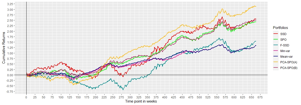
Figure 1: Cumulative returns of the portfolios from PCA-SPO(A), PCA-SPO(B), SPO, SSD, F-SSD, Min-var and Mean-var for S&P BSE 500 Market (India) for 3 month out-of-sample period (rolling window scheme)

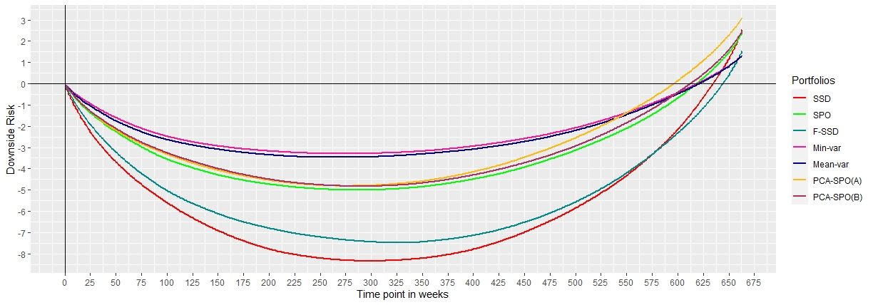
Figure 2: Downside Risk of the portfolios from PCA-SPO(A), PCA-SPO(B), SPO, SSD, F-SSD, Min-var and Mean-var for S&P BSE 500 Market (India) for 3 month out-of-sample period (rolling window scheme)

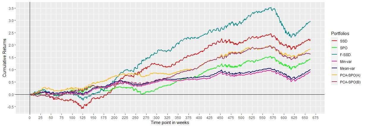
Figure 3: Cumulative returns of the portfolios from PCA-SPO(A), PCA-SPO(B), SPO, SSD, F-SSD, Min-var and Mean-var for S&P 500 Market (U.S.) for 3 month out-of-sample period (rolling window scheme)

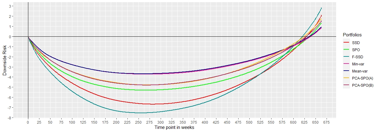
Figure 4: Downside Risk of the portfolios from PCA-SPO(A), PCA-SPO(B), SPO, SSD, F-SSD, Min-var and Mean-var for S&P 500 Market (U.S.) for 3 month out-of-sample period (rolling window scheme)

Figures 1 and 3 depict the out-of-sample cumulative returns of all the portfolios over the data sets, S&P BSE 500 and S&P 500, respectively. The main points of observations recorded from these figures are as follows:

1. From the Figure 1, portfolios from SSD dominates all till 130th week, followed by PCA-SPO(B). While portfolios from PCA-SPO(A) clocks the least return for first 130 weeks, it however increases thereafter and dominates all other portfolios from the 225th week. Portfolios from F-SSD suffers with the most negative returns and spots the least returns from 150th week to the 415th week.

2. From the Figure 3, the portfolios from PCA-SPO(A) dominates all portfolios till 210th week, while SSD suffers with the least returns (most negative returns) during this phase. SPO, on the other hand suffers with the least return from 200th week to 340th week. Portfolios from SSD, F-SSD, PCA-SPO(A), PCA-SPO(B) and SPO observe a rise (with F-SSD dominating) from 325th week till 575th week during the bullish phase of the market, indicating the dominance of expected returns over FRs. However, both SSD and F-SSD also observe a sharp fall during the bearish phase from 575th week to 615th week, with a drop of 1.25 cumulative returns, while the portfolios from remaining models drop only by 0.6.

3. We further note that the portfolios from PCA-SPO(B) never achieve least return over the considered time horizon for both the markets indicating the safer portfolio for the loss averse investors. In comparison to the SPO, PCA-SPO(A) always outperforms it, while PCA-SPO(B) outperforms SPO for S&P 500 and depicts similar return movement as the SPO over S&P BSE 500, highlighting the importance of selection of dominant ratios using PCA.

Figures 2 and 4 depicts the downside risk pattern from all the models over the S&P BSE 500 (India) and S&P 500 (U.S.) markets, respectively. We record the following main points from these figures:

1. We observe that the downside risk graphs corresponding to the models F-SSD and SSD are falling below in comparison to all other models for both the markets, indicating higher downside risk from these models, while those from the models Min-var and Mean-var stand above all other models (for both the markets) suggesting lowest downside risk from these models.

2. The downside risk graphs from the models SPO, PCA-SPO(A), and PCA-SPO(B) are found hanging above than the models SSD and F-SSD, highlighting the relevance of FRs and the two-step sector-wise implementation over the one-step F-SSD model.

3. Further, the better downside risk graphs from PCA-SPO(A) and PCA-SPO(B) in comparison to SPO highlights the relevance of selecting critical ratios for the sectors when FRs are considered.

To summarize, the proposed strategies PCA-SPO(A) and PCA-SPO(B) demonstrates overall best performance in terms of both risk as well return-risk measures. While SSD and F-SSD outperforms in terms of return, they however prove to be the most risky. On the other hand, Mean-var and Min-var depict better performance in terms of risk, however fail to impress in terms of return and performance ratios. Thus, the results from the rolling window scheme validates the proposed strategies PCA-SPO(A) and PCA-SPO(B), highlighting the importance of FRs, their sector-wise selection using PCA and the two-step implementation in the portfolio selection process.

5.3.2 Market phase wise out-of-sample analysis

For a comprehensive analysis of the proposed strategies with the existing models, we conduct the out-of-sample analysis on three different phases (price movements) of the market: neutral, bullish and bearish. For this, we first plot the cumulative returns graph for each of the index and identify cuts corresponding to the three phases graphically. Figures 5 and 6 show the labels for different market phases for the indices S&P BSE 500 (India) and S&P 500 (U.S.) respectively over the time horizon of 6 years from April 2014 to March 2020.

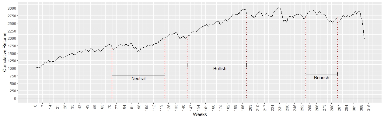
Figure 5: Cumulative Returns for S&P BSE 500 Index (India)

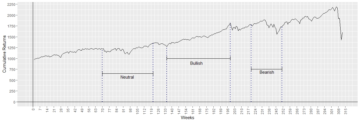
Figure 6: Cumulative Returns for S&P 500 Index (U.S.)

Each of the labelled scenario (neutral, bullish and bearish) is observed as out-of-sample period (testing period) and the corresponding previous year (52 weeks) is considered as the in-sample period (training period) for both the indices. All models are solved over the in-sample period and the portfolios thus obtained are tested over the identified phases on the basis of the performance measures mentioned in Section 5.1.

Table 11: Out-of-sample performance analysis of optimal portfolios generated from the model for neutral market scenario

Portfolios	SSD	SPO	Min-Var	Mean-Var	PCA-SPO(A)	PCA-SPO(B)	F-SSD
S&P BSE 500
Mean Return	0.00033	0.00182	0.00153	$-0.00240$	0.00200	0.00248	$-0.00029$
Sharpe Ratio	0.00941	0.06793	0.07917	—–	0.07225	0.09047	—–
Sortino Ratio	0.01346	0.10104	0.10954	—–	0.09972	0.12687	0.00000
DD	0.02457	0.01802	0.01399	0.02985	0.02003	0.01954	0.02156
VaR0.95	0.06096	0.04029	0.03067	0.06121	0.03685	0.03477	0.04896
VaR0.97	0.06407	0.04574	0.04188	0.08558	0.07083	0.06414	0.06068
CVaR0.95	0.07696	0.05001	0.03858	0.08876	0.06221	0.05780	0.06807
CVaR0.97	0.08496	0.05487	0.04254	0.010253	0.07489	0.06931	0.07763
STARR0.95	0.00430	0.03640	0.03972	—–	0.03211	0.04290	—–
STARR0.97	0.00389	0.03318	0.03602	—–	0.02667	0.03577	—–
Rachev0.95	0.87265	1.20308	0.99457	0.97704	0.93078	0.97278	0.70815
Rachev0.97	0.80938	1.24301	1.01783	0.91585	0.85679	0.91257	0.63054
S&P 500
Mean Return	0.00001	0.00195	0.00191	0.00142	0.00356	0.00309	-0.00078
Sharpe Ratio	0.00046	0.06844	0.11154	0.04126	0.13519	0.11029	0.00000
Sortino Ratio	0.00063	0.09048	0.14412	0.06224	0.17136	0.14108	0.00000
DD	0.02108	0.02157	0.01327	0.02286	0.02079	0.02188	0.01851
VaR0.95	0.05758	0.06328	0.03606	0.05066	0.04922	0.04447	0.04524
VaR0.97	0.06245	0.06863	0.04104	0.07241	0.06057	0.04689	0.04932
CVaR0.95	0.06355	0.06773	0.04082	0.06843	0.06715	0.06410	0.06428
CVaR0.97	0.06654	0.06996	0.04319	0.07731	0.07611	0.07392	0.07814
STARR0.95	0.00021	0.02882	0.04685	0.02079	0.05304	0.04816	0.00000
STARR0.97	0.00020	0.02790	0.04427	0.01840	0.04680	0.04176	0.00000
Rachev0.95	0.79001	0.74628	0.69671	1.22702	0.66233	0.63831	0.82042
Rachev0.97	0.78460	0.80210	0.69115	1.31646	0.61109	0.56506	0.80262

Table 11 records the performance of the portfolios for neutral out-of-sample phase for the indices S&P BSE-500 (India) and S&P 500 (U.S.). Following observations are drawn from Table 11:

1. For the Indian S&P BSE 500 index, PCA-SPO(B) performs best in terms of mean return, Sharpe, Sortino and STARR_0.95 values, while for the S&P 500 index, PCA-SPO(A) outperforms all other models in terms of mean return and the three ratios.

2. Both the PCA-SPO(A) and PCA-SPO(B) outperform SSD and SPO in terms of mean return, Sharpe, Sortino, VaR_0.95, VaR_0.97, CVaR_0.95 and STARR values for both the indices, highlighting the importance of FRs and the relevance of selecting critical ratios for each sector using PCA.

3. Portfolios from the Min-var model performs best in terms of risk measures by recording the least values of DD, VaR and CVaR values for both data sets, but does not impress much in terms of return-risk ratios.

4. Portfolios from the F-SSD model generates negative mean returns for both the data sets and thus suffers with the lowest values of Sharpe, Sortino and STARR ratios. In terms of risk measures, the portfolios from Mean-var models record the largest values of DD, VaR_0.95, VaR_0.97, CVaR_0.95 and CVaR_0.97 for S&P BSE 500 and of DD, VaR_0.97 and CVaR_0.95 for S&P 500 data set.

5. Portfolios from SSD and F-SSD also exhibit poor performance in terms of risk measures as well as the return-risk ratios, viz., Sharpe, Sortino, STARR and Rachev ratios.

6. None of the proposed strategies PCA-SPO(A) or PCA-SPO(B) perform worst in terms of any of the risk measure, making them safe portfolios over the neutral phase of the market.

In a nutshell, both proposed strategies PCA-SPO(A) and PCA-SPO(B) prove favourable during the neutral phase of the market.

Table 12: Out-of-sample performance analysis of optimal portfolios generated from the model for bearish market scenario

Portfolios	SSD	SPO	Min-Var	Mean-Var	PCA-SPO(A)	PCA-SPO(B)	F-SSD
S&P BSE 500
Mean Return	0.00471	0.00503	0.00222	0.00878	0.00159	0.00426	0.00607
Sharpe Ratio	0.20848	0.27304	0.11545	0.24921	0.08654	0.246720	0.28483
Sortino Ratio	0.30656	0.38065	0.16069	0.41441	0.12028	0.36041	0.38619
DD	0.01535	0.01322	0.01381	0.02119	0.01321	0.01182	0.01572
VaR0.95	0.02299	0.02188	0.02014	0.03748	0.02719	0.02051	0.03591
VaR0.97	0.03083	0.02384	0.02440	0.04053	0.03082	0.02545	0.04745
CVaR0.95	0.03252	0.02683	0.03232	0.04294	0.03057	0.02390	0.05378
CVaR0.97	0.03728	0.02931	0.03841	0.04567	0.03225	0.02559	0.05103
STARR0.95	0.14475	0.18758	0.06866	0.20451	0.05197	0.17827	0.11291
STARR0.97	0.12625	0.17171	0.05777	0.19229	0.04926	0.16646	0.11900
Rachev0.95	1.42063	1.31205	1.07080	1.90883	0.98161	1.45688	1.61128
Rachev0.97	1.42651	1.39050	0.95888	2.03490	0.98576	1.45545	0.95994
S&P 500
Mean Return	$-0.00590$	$-0.00187$	$-0.00285$	$-0.01191$	$-0.00420$	$-0.00418$	$-0.00658$
Sharpe Ratio	—–	—–	—–	—–	—–	—–	—–
Sortino Ratio	—–	—–	—–	—–	—–	—–	—–
DD	0.02800	0.02562	0.01823	0.05565	0.02273	0.02262	0.03891
VaR0.95	0.07243	0.06543	0.05112	0.10361	0.06344	0.05930	0.09534
VaR0.97	0.07808	0.06766	0.06882	0.26427	0.06944	0.06402	0.13045
CVaR0.95	0.09406	0.08318	0.07496	0.22992	0.08305	0.07708	0.14112
CVaR0.97	0.08133	0.07048	0.07168	0.27528	0.07233	0.06669	0.13589
STARR0.95	—–	—–	—–	—–	—–	—–	—–
STARR0.97	—–	—–	—–	—–	—–	—–	—–
Rachev0.95	0.71782	0.79315	0.56139	0.46747	0.80237	0.82596	0.69825
Rachev0.97	0.78877	0.79163	0.52777	0.41687	1.05939	0.88585	0.68115

Table 12 tracks down the performance of the portfolios for bearish out-of-sample phase for the indices S&P BSE-500 (India) and S&P 500 (U.S.). We draw the following observations from Table 12:

1. For the S&P BSE 500 dataset, though the Mean-var model exhibits better performance in terms of mean return, Sortino, STARR and Rachev ratios but records the highest values of DD and VaR_0.95 and second highest values of VaR_0.97, CVaR_0.95 and CVaR_0.97 after the F-SSD model. For the S&P 500 data set, it records the most negative mean return and highest values of DD, VaR_0.95, VaR_0.97, CVaR_0.95 and CVaR_0.97, proving to be the riskiest of all models considered along with the F-SSD and SSD model respectively, stand as the second and third most riskiest models. This hints that not using FRs at all or analyzing all stocks together on the basis of FRs may mislead the investor and result in loss during the bearish scenario.

2. PCA-SPO(B) records the lowest values of DD, CVaR_0.95, CVaR_0.97 and second lowest value of VaR_0.95 for S&P BSE 500, while for S&P 500, it records the lowest values of VaR_0.97 and CVaR_0.97 and second lowest values of DD and VaR_0.95, proving advantageous in terms of risk in a bearish scenario. Whereas, PCA-SPO(A) performs decently in terms of risk, it records the worst values of mean return, Sharpe, Sortino, STARR and Rachev ratios for S&P BSE 500, under performing in comparison to SPO and PCA-SPO(B), which hints the importance of each category of ratio when FRs are considered in portfolio selection.

3. Though the model SPO achieves higher mean return, Sharpe and Sortino values than PCA-SPO(B) but the later performs consistently well in terms of risk and Rachev ratios for both data sets. This hints the importance of each category of ratio and how choosing critical ratio using PCA can prove advantageous in terms of risk during a bearish scenario, where one aims to be risk-averse.

4. While the proposed strategy PCA-SPO(B) never generates worst values for any performance measures for both the data sets, PCA-SPO(A) fails to impress in bearish scenario, particularly for the Indian data set by recording worst values of mean return, Sharpe, Sortino, STARR and Rachev ratios.

To sum up, for a bearish scenario, where the primary aim of any investor is to protect the portfolio from extreme losses, the proposed strategy PCA-SPO(B) proves to be the most advantageous by winning over risk criteria and at the same time not generating poor returns.

Table 13: Out-of-sample performance analysis of optimal portfolios generated from the model for bullish market scenario

Portfolios	SSD	SPO	Min-Var	Mean-Var	PCA-SPO(A)	PCA-SPO(B)	F-SSD
S&P BSE 500
Mean Return	0.00831	0.00434	0.00298	0.00941	0.00965	0.00481	0.00807
Sharpe Ratio	0.28451	0.22015	0.27989	0.21523	0.37824	0.24348	0.32661
Sortino Ratio	0.40129	0.31834	0.46411	0.33365	0.56663	0.35434	0.49740
DD	0.02070	0.01362	0.00642	0.02821	0.01703	0.01357	0.01623
VaR0.95	0.03601	0.02962	0.01613	0.07264	0.02964	0.02155	0.03235
VaR0.97	0.06381	0.04153	0.02253	0.09424	0.03719	0.03715	0.03460
CVaR0.95	0.05544	0.04102	0.02188	0.09478	0.03593	0.03639	0.03977
CVaR0.97	0.06516	0.04673	0.02475	0.10584	0.03907	0.04381	0.04736
STARR0.95	0.14983	0.10571	0.13623	0.09930	0.26858	0.13215	0.20299
STARR0.97	0.12749	0.09280	0.12042	0.08892	0.26858	0.13215	0.20299
Rachev0.95	1.12171	1.04961	1.04004	1.13929	1.89863	1.21669	1.67022
Rachev0.97	0.98077	0.96266	0.93124	1.09607	1.88073	1.03221	1.60978
S&P 500
Mean Return	0.01156	0.00607	0.00475	0.02110	0.00586	0.00840	0.01227
Sharpe Ratio	0.47199	0.37377	0.49220	0.32891	0.35436	0.45482	0.44257
Sortino Ratio	0.69521	0.57807	0.68732	0.57574	0.53203	0.66145	0.06743
DD	0.01663	0.01050	0.00692	0.03664	0.01102	0.01269	0.01819
VaR0.95	0.03179	0.02591	0.00986	0.06728	0.02257	0.02158	0.03854
VaR0.97	0.03819	0.02679	0.01926	0.07895	0.02998	0.02928	0.04217
CVaR0.95	0.03391	0.02490	0.01500	0.07234	0.02591	0.02786	0.03873
CVaR0.97	0.04021	0.02820	0.01994	0.08606	0.03160	0.03537	0.04478
STARR0.95	0.34108	0.24388	0.31689	0.29165	0.22631	0.30132	0.31676
STARR0.97	0.28761	0.21528	0.23835	0.24514	0.18552	0.23736	0.27395
Rachev0.95	1.72434	1.75461	1.39755	2.79556	1.54505	1.70714	2.04578
Rachev0.97	1.71179	1.84416	1.19978	3.17779	1.52706	1.63193	2.06018

Table 13 documents the performance of the portfolios for bullish out-of-sample market scenario and the observations can be summarized as follows:

1. For the Indian S&P BSE 500 market, PCA-SPO(A) depicts superior performance in terms of mean return, Sharpe, Sortino, STARR and Rachev ratios but fails to perform the same over S&P 500 market.

2. The portfolios from Mean-var model outperforms in terms of mean return for both the data sets but proves to be the most risky by recording highest values of DD, VaR_0.95, VaR_0.97, CVaR_0.95 and CVaR_0.97 for both the data sets. In terms of risk, the Min-var model proves best; however achieves the worst values of mean return and Rachev ratios for both the data sets.

3. The portfolios from the F-SSD and SSD model achieves higher values of mean return, Sharpe and Sortino ratios in comparison to the portfolios from PCA-SPO(B); however also prove riskier than PCA-SPO(B) by recording higher values of DD, VaR_0.95, VaR_0.97, CVaR_0.95 and CVaR_0.97 with SSD recording the highest values over Indian data set and F-SSD over the U.S. data set.

4. The proposed strategy PCA-SPO(B) outperforms SPO for almost all performance measures and never achieves worst performance for any performance measure for both the data sets.

To summarize, for a bullish scenario, the aggressive (risk-taking) investors should opt for mean-variance or SSD or the F-SSD (when FRs are to be considered) whereas conservative (risk-averse) should opt for the minimum variance model. For the moderate investors however, PCA-SPO(B) proves to be the most advantageous that wisely employs financial analysis to avoid extreme risk and at the same time benefits from the rising return trend in a bullish scenario.

6 Managerial Implications

Our proposed strategy first filters significant objective functions made of financial ratios for each sector via PCA and then apply an optimization tools to find out the optimal weights for each stock and thus helping portfolio managers and investors with a sophisticated portfolio selection strategy. The applications of this study, however, is not just limited to portfolio management but has important implementations for accountants, business analysts, financial analysts, researchers and academicians. The proposed strategy can be exploited as a whole by a portfolio analyst who is focusing on a diversified investment across all sectors by utilizing the fundamental analysis with the help of financial ratios in the investment process. Nonetheless, each step of the strategy has an individual applicability in various domains. For instance, Step 1 that uses PCA to filter out relevant ratios can be used by practitioners for determining the most significant factors from a large set of variables for various purposes like assessment of risk, forecasting failures, predicting future profits, and many more. Additionally, Step 2 that determines an optimal portfolio for each sector can be utilized by portfolio managers and financial analysts to filter out elite stocks from each sector. Analogous to this, banks can utilize this step for loan assessment. This step can help banking analysts to filter out A-list businesses to grant loan to. Thus, the proposed research has managerial implications for portfolio management, forecasting and predictive analysis, banking and education.

7 Conclusion

The importance of FA in portfolio framework can not be overlooked. However, the right choice of ratios and their correct usage is even more crucial, owing to the fact that companies belonging to different industry sectors have different operational structures and business functionalities.

The SPO model aptly considers the sector-wise implementation but chooses ratios common for all sectors. This paper is an attempt forward on improvising the SPO model by implementing PCA for the selection of critical ratios for each sector, extracted in two ways, one from the components (strategy named as PCA-SPO(A)) and other from each category of ratios on the basis of communalities (strategy named as PCA-SPO(B)). We conduct the comparative analysis on the proposed strategies, PCA-SPO(A) and PCA-SPO(B), with the models Mean-var, Min-var, F-SSD, SSD, and SPO in two ways, viz., a rolling window scheme and second using scenario based analysis.

The rolling window analysis which is carried over the out-of-sample of 3 months showed that the optimal portfolios obtained from the proposed strategies PCA-SPO(A) and PCA-SPO(B) resulted in lower values of risk measures and generated better risk-reward profile in terms of Sortino, Sharpe, Rachev, and STARR ratios in comparison to other models for both the data sets considered in the study. On the other hand, the scenario based analysis which is carried over three different phases of the market, viz., neutral, bullish and bearish endorses the proposed strategy PCA-SPO(B). While for the bullish scenario, PCA-SPO(B) proves promising for the moderate investors only, it however proves propitious for all types of investors for both neutral and bearish scenarios.

To sum up, the proposed strategy PCA-SPO(B) is an apt decision making process that focuses primarily on the extraction of critical ratios from each category by employing PCA sector wise and then generates final portfolio incorporating the two step SPO model. The financial benefits of PCA-SPO(B) over SPO and other models confirms the practical usage of the proposed strategy. Further extensions of the present work are possible by including other important factors like technical indicators, sustainability, socio-economic variables, and transaction costs in the portfolio framework.

References

- Arkan (2016) Arkan, T. (2016) The importance of financial ratios in predicting stock price trends: A case study in emerging markets. Zeszyty Naukowe Uniwersytetu Szczecińskiego Finanse Rynki Finansowe Ubezpieczenia, 1(1), 13–26.
- Baydar et al. (2002) Baydar, N., Ball, A., & Payne, B. (2002) Detection of incipient gear failures using statistical techniques, IMA Journal of Management Mathematics, 13(1), 71–79, https://doi.org/10.1093/imaman/13.1.71.
- Beaver (1966) Beaver, W.H. (1966) Financial ratios as predictors of failure. Journal of Accounting Research, 4, 71–111.
- Bruni et al. (2012) Bruni, R., Cesarone, F., Scozzari, A., & Tardella, F. (2012) A new stochastic dominance approach to enhanced index tracking problems. Economic Bulletin, 32(4), 3460–3470.
- Chen and Shimerda (1981) Chen, K.H., & Shimerda, T.A. (1981) An empirical analysis of useful financial ratios. Financial Management, 10(1), 51–60.
- Chowdhury et al. (2018) Chowdhury, U., Chakravarty, S., & Hossain, M. (2018) Short-term financial time series forecasting integrating principal component analysis and independent component analysis with support vector regression. Journal of Computer and Communications, 6(3), 51–67.
- Delen et al. (2013) Delen, D., Kuzey, C., & Uyar, A. (2013) Measuring firm performance using financial ratios: A decision tree approach. Expert Systems with Applications, 40(10), 3970–3983.
- Deng et al. (2021) Deng, S., Wang, C., Fu, Z. et al. (2021) An Intelligent System for Insider Trading Identification in Chinese Security Market. Computational Economics, 57, 593–616. https://doi.org/10.1007/s10614-020-09970-8
- Dentcheva and Ruszczyński (2003) Dentcheva, D., & Ruszczyński, A. (2003) Optimization with stochastic dominance constraints. SIAM Journal on Optimization, 14(2), 548–566.
- Dentcheva and Ruszczyński (2006) Dentcheva, D., & Ruszczyński, A. (2006) Portfolio optimization with stochastic dominance constraints. Journal of Banking and Finance, 30(2), 433–451.
- Edirisinghe and Zhang (2007) Edirisinghe, N.C.P., & Zhang, X. (2007) Generalized DEA model of fundamental analysis and its application to portfolio optimization. Journal of Banking and Finance, 31(11), 3311–3335.
- Edirisinghe and Zhang (2008) Edirisinghe, N.C.P., & Zhang, X. (2008) Portfolio selection under DEA-based relative financial strength indicators: case of us industries. Journal of the Operational Research Society, 59(6), 842–856.
- Fabian et al. (2011) Fabian, C., Mitra, G., & Roman, D. (2011) Processing second order stochastic dominance models using cutting-plane representations. Mathematical Programming, 130, 33–57.
- Fang et al. (2018) Fang, L., Xiao, B., Yu, H., & You, Q. (2018) A stable systemic risk ranking in China’s banking sector: Based on principal component analysis. Physica A: Statistical Mechanics and its Applications, 492, 1997–2009.
- Fidan Kececi et al. (2016) Fidan Kececi, N., Kuzmenko, V., & Uryasev, S. (2016) Portfolios dominating indices: Optimization with second-order stochastic dominance constraints vs. minimum and mean variance portfolios. Journal of Risk and Financial Management, 9(4), 11, https://doi.org/10.3390/jrfm9040011.
- Fulga and Dedu (2012) Fulga, C., & Dedu, S. (2012) Mean-risk portfolio optimization with prior PCA-based stock selection. In: The International Workshop Stochastic Programming for Implementation and Advanced Applications, vol Stochastic Programming for Implementation and Advanced Applications.
- Ghorbani and Chong (2020) Ghorbani, M., & Chong, E.K. (2020) Stock price prediction using principle components. PLOS ONE, 15(3), 1–20.
- Giuliani (2017) Giuliani, A. (2017) The application of principal component analysis to drug discovery and biomedical data. Drug Discovery Today, 22(7), 1069–1076.
- Goel and Sharma (2019) Goel, A., & Sharma, A. (2019). Deviation measure in second-order stochastic dominance with an application to enhanced indexing. International Transactions in Operational Research, 28, 2218–2247.
- Graham (1949) Graham, B. (1949) The intelligent investor. New York: Harper & Bothers.
- Graham and Dodd (1934) Graham, B., & Dodd, D. (1934) Security Analysis. New York: Whittlesey House McGraw-Hill Book Co.
- Guran et al. (2019) Guran, C., Ugurlu, U., & Taş, O.(2019) Mean-variance portfolio optimization of energy stocks supported with second order stochastic dominance efficiency. Finance a Uver, 69, 366–383.
- Hadar and Russell (1969) Hadar, J., & Russell, W. (1969) Rules for ordering uncertain prospects. The American Economic Review, 59(1), 25–34.
- Hernandez and Méndez (2018) Hernandez, W., & Méndez, A. (2018) Statistics: Growing Data Sets and Growing Demand for Statistics, United Kingdom: IntechOpen., chap Application of Principal Component Analysis to Image Compression.
- Hotelling (1933) Hotelling, H. (1933) Analysis of a complex of statistical variables into principal components. Journal of Educational Psychology, 24(7), 498–520.
- Huang et al. (2014) Huang, C.Y., Chiou, C.C., Wu, T.H., & Yang, S.C. (2014) An integrated DEA-MODM methodology for portfolio optimization. Operational Research, 15, 115–136.
- Jagannathan and Ma (2003) Jagannathan, R., & Ma, T. (2003) Risk reduction in large portfolios: Why imposing wrong constraints helps. Journal of Finance, 58, 1651–1684.
- Joldes (2018) Joldes, C. (2018). The selection of stocks using principal component analysis. In: International Conference on Economics, Business and Economic Thought. https://doi.org/10.31410/itema.2018.454.
- Jothimani et al. (2017) Jothimani, D., Shankar, R., & Yadav, S. (2017) A PCA-DEA framework for stock selection in Indian stock market. Journal of Modelling in Management, 12, 386–403.
- Konno and Suzuki (1995) Konno, H., & Suzuki, K. (1995) A mean-variance-skewness portfolio optimization model. Journal of Operational Research Society of Japan, 38, 173–187.
- Konno et al. (1993) Konno, H., Shirakawa, H., & Yamazaki, H. (1993) A mean-absolute deviation-skewness portfolio optimisation model. Annals of Operations Research, 45, 205–220.
- Kopa et al. (2022) Kopa,M., Kabašinskas, A., & Šutienė, K. (2022) A stochastic dominance approach to pension-fund selection, IMA Journal of Management Mathematics, 33(1), 139–160, https://doi.org/10.1093/imaman/dpab002.
- Kouaissah and Lozza (2021) Kouaissah, N. & Lozza, S.O. (2021) Multivariate stochastic dominance applied to sector-based portfolio selection, IMA Journal of Management Mathematics, 32(2), 139–160, https://doi.org/10.1093/imaman/dpaa004
- Leshno and Levy (2002) Leshno, M., & Levy, H. (2002) Preferred by all and preferred by most decision makers: almost stochastic dominance. Management Science, 48(8), 1074–1085.
- Levy (1992) Levy, H. (1992) Stochastic dominance and expected utility: Survey and analysis. Management Science, 38, 555–593.
- Lv et al. (1992) Lv, J., Xiao, Z.H., & Pang, L.P. (1992) An incremental bundle method for portfolio selection problem under second-order stochastic dominance. Numerical Algorithms, 85, 653–681.
- Markowitz (1952) Markowitz, H. M. (1952) Portfolio selection. Journal of Finance, 7, 77–91.
- Marshall and Olkin (1979) Marshall, A.W., & Olkin, I. (1979) Inequalities: Theory of majorization and its applications. San Diego: Academic Press.
- Nadkarni and Neves (2018) Nadkarni, J., & Neves, R.F. (2018) Combining neuro-evolution and principal component analysis to trade in the financial markets. Expert Systems with Applications, 103, 184–195.
- Ocal et al. (2007) Ocal, M., Oral, E., Erdis, E., & Vera, G. (2007) Industry financial ratios-application of factor analysis in turkish construction industry. Building and Environment, 42, 385–392.
- Olufemi et al. (2012) Olufemi, A., Fajembola, O., & Olopete, M. (2012) Predicting bank failure in Nigeria using principal component analysis and D-score model. Research Journal of Finance and Accounting, 3, 159–170.
- Pearson (1901) Pearson, K. (1901) On lines and planes of closest fit to systems of points in space. Philosophical Magazine, 2, 559–572.
- Pinches et al. (1973) Pinches, G., Mingo, K., & Caruthers, J. (1973) The stability of financial patterns in industrial organizations. Journal of Finance, 28(3), 389–396.
- Quirk and Saposnik (1962) Quirk, J., & Saposnik, R. (1962) Admissibility and measurable utility functions. Review of Economic Studies, 29, 140–146.
- Roman and Mitra (2009) Roman, D., & Mitra, G. (2009) Portfolio selection models:a review and new directions. Wilmott Journal, 1(2), 69–85.
- Roman et al. (2006) Roman, D., Darby, D.K., & Mitra, G. (2006) Portfolio construction based on stochastic dominance and target return distributions. Mathematical Programming, 108, 541–569.
- Roman et al. (2013) Roman, D., Mitra, G., & Zverovich, V. (2013) Enhanced indexation based on second order stochastic dominance. European Journal of Operational Research, 228, 273–281.
- Samaras et al. (2008) Samaras, G., Matsatsnis, N., & Zopounidis, C. (2008) A multi criterion DSS for stock evaluation using fundamental analysis. European Journal of Operational Research, 187(3), 1380–1401.
- Sehgal and Mehra (2020) Sehgal, R., & Mehra, A. (2020) Robust portfolio optimization with second order stochastic dominance constraint. Computers & Industrial Engineering, 144, 106396.
- Sharma and Mehra (2013) Sharma, A., & Mehra, A. (2013) Portfolio selection with a minimax measure in safety constraint. Optimization, 62(11), 1473–1500 .
- Sharma and Mehra (2015) Sharma, A., & Mehra, A. (2015) Extended omega ratio optimization for risk-averse investors. International Transactions in Operational Research, 24, 485–506.
- Sharma and Mehra (2017) Sharma, A., & Mehra, A. (2017) Financial analysis based sectoral portfolio optimization under second order stochastic dominance. Annals of Operations Research, 256, 171–197.
- Sharma et al. (2017) Sharma, A., Agrawal, S., & Mehra, A. (2017) Enhanced indexing for risk averse investors using relaxed second order stochastic dominance. Optimization and Engineering, 18, 407–442.
- Silva et al. (2014) Silva, A., Neves, R., & Horta, N. (2014) A hybrid approach to portfolio composition based on fundamental and technical indicators. Expert Systems with Applications, 42(4), 2036–2048.
- Singh and Dharmaraja (2017) Singh, A., & Dharmaraja, S. (2017) Optimal portfolio trading subject to stochastic dominance constraints under second order auto regressive price dynamics. International Transactions in Operational Research, 27(3), 1771–1803.
- Tan et al. (1997) Tan, P., Koh, H., & Low, L. (1997). Stability of financial ratios: A study listed companies in Singapore. Asian Review of Accounting, 5(1), 9–39.