A fullwave model of the nonlinear wave equation with multiple relaxations and relaxing perfectly matched layers for high-order numerical finite-difference solutions

Abstract

Large-scale simulations of the wave equation in electromagnetism, seismology, and acoustics, can be solved efficiently by finite difference methods. The accuracy of these numerical solutions usually depends on the minimization of dissipation and dispersion error using optimized schemes. However, these optimized schemes are often difficult to implement for more complex formulations of the wave equation. Here we present a model of the quadratically nonlinear wave equation with multiple relaxations as a function of space that can model perfectly matched layers and is designed to be easily used with optimized finite difference stencils on a staggered grid. Solutions are demonstrated in 2D and 3D for ultrasound imaging applications where the long propagation lengths, heterogeneous media in the human body, large dynamic range, and requirements for computational speed, demonstrate the utility of the proposed methods.

I Introduction

Large-scale acoustic simulations of wave propagation require efficient and accurate algorithms. In the past decades many finite-difference (FD) methods have been developed for wave propagation in seismology and acoustics [1, 2]. Staggered-grid FD is often associated with higher stability in heterogeneous media with large contrast and is in may cases more accurate than methods implemented on a conventional grid [3, 4, 5]. Given their ease of implementation, speed, parallelizability, and accuracy, staggered grid finite differences are used extensively in electromagnetism, seismology, and acoustics.

Acoustic wave propagation in ultrasound imaging involves several physical phenomena: diffraction, reflection, scattering, frequency dependent attenuation, and nonlinearity. A direct simulation of acoustic wave propagation to a target, reflection, and propagation back to a transducer is constrained by two fundamental physical scales: i) the propagation distance ($\sim 100\lambda$) and ii) sub-resolution scatterers ($<\lambda/10$). To represent both length scales in 3D, simulation fields with large number of points in space ($\sim 10^{9}$) are required. Furthermore, numerical methods are challenged by the extremely high dynamic range because the backscattered wave may be 100 dB smaller than the transmitted pulse.

For long-range propagation on coarse grids, one of the main challenges for FD is controlling numerical error, usually in the form of space and time dispersion [5]. Here we present a formulation of the wave equation that can model nonlinearity, arbitrary attenuation laws, and that can be used with high-order stenciles that are optimized to minimize dispersion and dissipation errors. Relexation mechanisms that are heterogeneous as a function of space are used to describe the attenuation laws in tissue and also to implement convolutional perfectly matched layers. We then conduct numerical modeling of scalar wave propagation in 2D and 3D complex media in the context of ultrasound imaging applications where the long propagation lengths, heterogeneous media in the human body, large dynamic range, and requirements for computational speed, demonstrate the utility of the proposed methods. Results are validated experimentally and theoretically.

II Methods

II-A Linear attenuation and dispersion

The pressure-velocity formulation of the wave equation can be written as

$$\mathbf{\nabla}p+\rho\frac{\partial\mathbf{v}}{\partial t}=0$$ (1)

$$\mathbf{\nabla}\cdot\mathbf{v}+\kappa\frac{\partial p}{\partial t}=0$$ (2)

where $p(\mathbf{x},t)$ is the pressure, $\mathbf{v}(\mathbf{x},t)=(u(\mathbf{x},t),v(\mathbf{x},t),w(\mathbf{x},t))^{T}$ is the vector of the velocity wavefield, $\rho(\mathbf{x})$ is the density, $\kappa(\mathbf{x})$ is the compressibility. Attenuation typically included by added relaxation mechanisms to the equation of state.

To preserve the structure of this system of equations the attenuation and dispersion is modeled by a complex coordinate transformation of the spatial derivatives. Furthermore, this transformation is independent for the spatial derivatives in Eq. 1 and Eq. 2. This coordinate transformation is introduced by complex coordinate transformation of the spatial derivatives that are denoted by $\mathbf{\nabla}_{1}$ and $\mathbf{\nabla}_{2}$, i.e.

$$\mathbf{\nabla}_{1}p+\rho\frac{\partial\mathbf{v}}{\partial t}=0$$ (3)

$$\mathbf{\nabla}_{2}\cdot\mathbf{v}+\kappa\frac{\partial p}{\partial t}=0$$ (4)

This can be written as a scaling of the partial derivative and a sum on convolutions with $N$ relaxation functions, which for $\mathbf{\nabla}_{1}$ can be written as

$$\frac{\partial}{\partial\tilde{x_{1}}}=\frac{1}{\kappa_{x_{1}}}\frac{\partial}{\partial x}+\sum_{\nu=1}^{N}\zeta_{x_{1}}^{\nu}(t)\ast\frac{\partial}{\partial x}$$ (5)

$$\frac{\partial}{\partial\tilde{y_{1}}}=\frac{1}{\kappa_{y_{1}}}\frac{\partial}{\partial y}+\sum_{\nu=1}^{N}\zeta_{y_{1}}^{\nu}(t)\ast\frac{\partial}{\partial y}$$ (6)

$$\frac{\partial}{\partial\tilde{z_{1}}}=\frac{1}{\kappa_{z_{1}}}\frac{\partial}{\partial z}+\sum_{\nu=1}^{N}\zeta_{z_{1}}^{\nu}(t)\ast\frac{\partial}{\partial z}$$ (7)

and where convolution kernels for the $N$ relaxations, indexed by $\nu$, are

$$\zeta_{x_{1}}^{\nu}(t)=-\frac{d_{x_{1}}^{\nu}}{\kappa_{x_{1}}^{2}}e^{-(d_{x_{1}}^{\nu}/\kappa_{x_{1}}+\alpha_{x_{1}}^{\nu})t}H(t)$$ (8)

$$\zeta_{y_{1}}^{\nu}(t)=-\frac{d_{y_{1}}^{\nu}}{\kappa_{y_{1}}^{2}}e^{-(d_{y_{1}}^{\nu}/\kappa_{y_{1}}+\alpha_{y_{1}}^{\nu})t}H(t)$$ (9)

$$\zeta_{z_{1}}^{\nu}(t)=-\frac{d_{z_{1}}^{\nu}}{\kappa_{z_{1}}^{2}}e^{-(d_{z_{1}}^{\nu}/\kappa_{z_{1}}+\alpha_{z_{1}}^{\nu})t}H(t)$$ (10)

Here $\kappa_{x_{1}}(\mathbf{x})$, $\kappa_{y_{1}}(\mathbf{x})$, $\kappa_{z_{1}}(\mathbf{x})$, represent a linear scaling of the derivative that is outside of the convolution and is consequently a memoryless parameter. This scaling simply modifies the overall wave speed in the $x$, $y$, and $z$ directions. Note that these variables vary as a function of their position in space, $\mathbf{x}$. The variables $d^{\nu}_{x_{1}}(\mathbf{x})$, $d^{\nu}_{y_{1}}(\mathbf{x})$, and $d^{\nu}_{z_{1}}(\mathbf{x})$ represent a scaling-dependent damping profile; and $\alpha^{\nu}_{x_{1}}(\mathbf{x})$, $\alpha^{\nu}_{y_{1}}(\mathbf{x})$, $\alpha^{\nu}_{z_{1}}(\mathbf{x})$, represent a scaling-independent damping profile. Here $H(t)$ is the Heaviside or unit step function. In an isotropic material these constants do not depend on the $x$, $y$, and $z$ directions, however in general they can vary independently. This fact will facilitate the description of relaxing PMLs, as will be shown subsequently. The relaxation transformation $\mathbf{\nabla}_{1}$ for Eq. 3 is associated with the compressibility attenuation in acoustic media.

An identical set of transformations, not shown here, can be applied to $\nabla_{2}$ in Eq. 4 . Variables associated with this second transformation are denoted by the subscript 2. This relaxation transformation of $\mathbf{\nabla}_{2}$ is generally zero for an acoustic medium but, by analogy with solid mechanics, it could be associated with a damping term that is proportional to the mass [6]. Although they can be associated to physical processes, here these relaxation mechanisms are used to model attenuation empirically, based on observations of the attenuation laws and parameters observed in soft tissue. The relaxation mechanisms are generalizable to arbitrary attenuation laws via a fitting process of the relaxation constants.

When the coordinate transformations are applied in the same manner to Eqs. (1) and (2), i.e. $\mathbf{\nabla}_{1}$ = $\mathbf{\nabla}_{2}$, the system is dispersionless but attenuating, which is the fundamental behavior that governs PMLs. For example, for the case where $\nu=1$, $\kappa_{x_{1}}=\kappa_{x_{2}}=1$, and $\alpha_{x_{1}}=\alpha_{x_{2}}=0$, we get the classical PML coordinate transformation. For the case where the case where the coordinate transformations are applied in the same manner to Eqs. (1) and (2), and $\nu=1$, $\kappa_{x_{1}}=\kappa_{x_{2}}$, and $\alpha_{x_{1}}=\alpha_{x_{2}}$ we get the C-PML coordinate transformation. In the general case when $\mathbf{\nabla}_{1}\neq\mathbf{\nabla}_{2}$ the coordinate stretching introduces dispersion into the system.

This dispersion and attenuation can be quantified with the implicit relationship describing the wavenumber, $k$

$$k=\frac{\omega}{c}\left(\frac{1}{\kappa_{x_{1}}\kappa_{x_{2}}}-\frac{\gamma_{1}}{\kappa_{x_{2}}}-\frac{\gamma_{2}}{\kappa_{x_{1}}}+\gamma_{1}\gamma_{2}\right)^{-1}$$ (11)

where $c=1/\sqrt{\kappa\rho}$ and where

$$\gamma_{1}=\sum_{\nu=1}^{N}\frac{d^{\nu}_{x_{1}}}{\kappa^{2}_{x_{1}}}\left(\frac{1}{d^{\nu}_{x_{1}}/\kappa_{x_{1}}+\alpha^{\nu}_{x_{1}}+i\omega}\right)$$ (12)

$$\gamma_{2}=\sum_{\nu=1}^{N}\frac{d^{\nu}_{x_{2}}}{\kappa^{2}_{x_{2}}}\left(\frac{1}{d^{\nu}_{x_{2}}/\kappa_{x_{2}}+\alpha^{\nu}_{x_{2}}+i\omega}\right)$$ (13)

If $\gamma_{1}=\gamma_{2}=0$ the dispersionless wavenumber for the lossless wave equation, $k=\omega/c$, is recovered.

Other coordinates stretched with their own independent or dependent transformations

II-B numerical solutions

In the 2D case the staggered-grid finite difference discretization of Eqs. (1) and (2) are given by

$$p_{0,0}^{n}=p_{0,0}^{n-1}-\frac{1}{\kappa}(D_{x}^{0}u_{0,0}^{n-1/2}+D_{y}^{0}v_{0,0}^{n-1/2})\Delta t$$ (14)

$$u_{1/2,0}^{n+1/2}=u_{1/2,0}^{n-1/2}-\frac{1}{\rho}D_{x}^{0}p_{1/2,0}^{n}\Delta t$$ (15)

$$v_{0,1/2}^{n+1/2}=v_{0,1/2}^{n-1/2}-\frac{1}{\rho}D_{y}^{0}p_{0,1/2}^{n}\Delta t$$ (16)

where $\Delta t$ is the time interval, $D_{x}^{0}$ and $D_{y}^{0}$ are finite difference operators along the $x$-axis and $y$-axis, respectively, $p_{m,n}^{j}$ is the discretized pressure wavefield $p(x+ih,y+jh,n\Delta t)$, $u_{i,j}^{n+1/2}$ and $v_{i,j}^{n+1/2}$ are the discretized velocity wavefields.

$$\frac{\partial p}{\partial x}\approx D_{x}^{2M,4}p_{0,0}^{n}=\frac{1}{h}\left[g_{1,1}(p_{1/2,1}^{n}-p_{-1/2,1}^{n}+p_{1/2,-1}^{n}-p_{-1/2,-1}^{n})+\sum_{i=1}^{M}g_{m,0}(p_{i-1/2,0}^{n}-p_{-i+1/2,0}^{n})\right]$$ (17)

The finite-difference operator $D_{x}^{2M,4}$ has $2M^{th}$-order accuracy in space and fourth order accuracy in time.

The first term in Eq. 5 can be computed by simply scaling the existing spatial derivative calculation. To compute the second term within the staggered grid finite difference formulation the convolutional operator can be solved numerically using exponential differentiation. This numerical approach simplifies the convolution operator, which theoretically requires storing all past time steps, by using auxilliary variables. The auxiliary variable acts as a memory variable that allows the convolution to be collapsed from a sum for all previous time to an update of the independent variable at the current time based on the memory variable.

The convolution term at time step $n$ for the derivative coordinate transformation of $\nabla_{1}$ in the $x$-coordinate is denoted by $\psi^{n}_{x_{1}}$. Then,

$$(\psi^{\nu}_{x_{1}})^{n}=\left(\zeta_{x_{1}}\ast\frac{\partial}{\partial x}\right)^{n}=\int^{n\Delta t}_{0}\left(\frac{\partial}{\partial x}\right)^{n\Delta t-\tau}\zeta_{x_{1}}(\tau)d\tau$$ (18)

Since the grid is staggered, the time integration scheme is defined half a time step between $m\Delta t$ and $(m+1)\Delta t$ so that:

$$(\psi^{\nu}_{x_{1}})^{n} =\sum_{m=0}^{n-1}\int^{(m+1)\Delta t}_{m\Delta t}\left(\frac{\partial}{\partial x}\right)^{n\Delta t-\tau}\zeta_{x_{1}}(\tau)d\tau$$ (19)

$$=\sum_{m=0}^{n-1}\left(\frac{\partial}{\partial x}\right)^{n-(m+1/2)}\int^{(m+1)\Delta t}_{m\Delta t}\zeta_{x_{1}}(\tau)d\tau$$ (20)

$$=\sum_{m=0}^{n-1}Z_{x_{1}}^{\nu}(m)\left(\frac{\partial}{\partial x}\right)^{n-(m+1/2)}$$ (21)

where

$$Z_{x_{1}}^{\nu}(m)=\int^{(m+1)\Delta t}_{m\Delta t}\zeta_{x_{1}}(\tau)d\tau$$ (22)

Then, using Eq. 8

$$Z_{x_{1}}^{\nu}(m) =-\frac{d_{x_{1}}^{\nu}}{\kappa_{x_{1}}^{2}}\int^{(m+1)\Delta t}_{m\Delta t}e^{-(d_{x_{1}}^{\nu}/\kappa_{x_{1}}+\alpha_{x_{1}}^{\nu})\tau}d\tau$$ (23)

$$=a_{x_{1}}^{\nu}e^{-(d_{x_{1}}^{\nu}/\kappa_{x_{1}}+\alpha_{x_{1}}^{\nu})m\Delta t}$$ (24)

where

$$a_{x_{1}}^{\nu}=\frac{d_{x_{1}}^{\nu}}{\kappa_{x_{1}}(d_{x_{1}}^{\nu}+\kappa_{x_{1}}\alpha_{x_{1}}^{\nu})}(b_{x_{1}}^{\nu}-1)$$ (25)

and

$$b_{x_{1}}^{\nu}=e^{-(d_{x_{1}}^{\nu}/\kappa_{x_{1}}+\alpha_{x_{1}}^{\nu})\Delta t}$$ (26)

From the numerical point of view, the memory and computational requirements are low because the memory variable $(\psi^{\nu}_{x_{1}})^{n}$ is updated at each time step by

$$(\psi^{\nu}_{x_{1}})^{n}=b_{x_{1}}^{\nu}(\psi^{\nu}_{x_{1}})^{n-1}+a_{x_{1}}^{\nu}\left(\frac{\partial}{\partial x}\right)^{n-1/2}$$ (27)

Then, each spatial derivative for the $x$-coordinate can in the $\nabla_{1}$ in Eq.4 be replaced by

$$\frac{\partial}{\partial\tilde{x}}=\frac{1}{\kappa_{x_{1}}}\frac{\partial}{\partial x}+\sum_{\nu=1}^{M}\psi^{\nu}_{x_{1}}$$ (28)

Identical calculations will lead to equivalent expressions for $\frac{\partial}{\partial\tilde{y}}$ and $\frac{\partial}{\partial\tilde{z}}$. The coefficients for the relaxation in $x$, $y$, and $z$ do not need to be identical, in which case the relaxation is anisotropic.

II-C Nonlinear propagation

Propagation in a nonlinear isotropic, lossless fluid can be described by a system of first order acoustic equations [7]

$$\mathbf{\nabla}p+\rho D_{t}\mathbf{v}=0$$ (29)

$$\mathbf{\nabla}\cdot\mathbf{v}+\kappa D_{t}p=0$$ (30)

where $p$ is the acoustic pressure, $\mathbf{v}$ is the particle velocity, and $D_{t}=\partial_{t}+\mathbf{v}\cdot\mathbf{\nabla}$ denotes the total or material derivative. The medium properties are determined by the density $\rho$, and the compressibility $\kappa$. The nonlinear behavior can be a consequence of terms in the material derivative or the equation of state of the medium. The equation of state, up to a second order terms in Eqs. (29) and (30), can be written as [7]

$$\rho=\rho_{0}[1+\kappa_{0}p]$$ (31)

$$\kappa=\kappa_{0}[1+\kappa_{0}(1-2\beta)p]$$ (32)

where $\rho_{0}$ is the equilibrium density, $\kappa_{0}$ is the equilibrium compressibility, and $\beta=1+B/2A$ is the coefficient of nonlinearity. By neglecting third order products of $p$ and/or $\mathbf{v}$ and the locally nonlinear terms given by $\mathbf{v}\cdot\nabla\mathbf{v}$ and $\mathbf{v}\cdot\nabla p$ Eqs. (29)- (32) lead to

$$\mathbf{\nabla}p+\rho_{0}[1+\kappa_{0}p]\frac{\partial\mathbf{v}}{\partial t}=0$$ (33)

$$\mathbf{\nabla}\cdot\mathbf{v}+\kappa_{0}[1+\kappa_{0}(1-2\beta)p]\frac{\partial p}{\partial t}=0$$ (34)

Note that by further removing all locally nonlinear terms this system of equations can be reduced to the well-known Westervelt equation [8].

II-D Numerical implementation and validation

The relaxation parameters where fitted to a linear relaxation law $\alpha=0.5$ dB/MHz/cm that is representative of soft tissue in the human body (Fig. 1, left). The dispersion (Fig. 1, right), associated with this attenuation law was calculated analytically using the Kramers Kronig dispersion relation which relates attenuation and dispersion using the principle of causality [9]. Then the relaxation parameters for three relaxation mechanisms in an isotropic medium were fitted to the analytical law using a minimization of the mean square error. The numerical fit of the attenuation and dispersion is shown as the solid line in Fig. 1 across a range of 1-10 MHz.

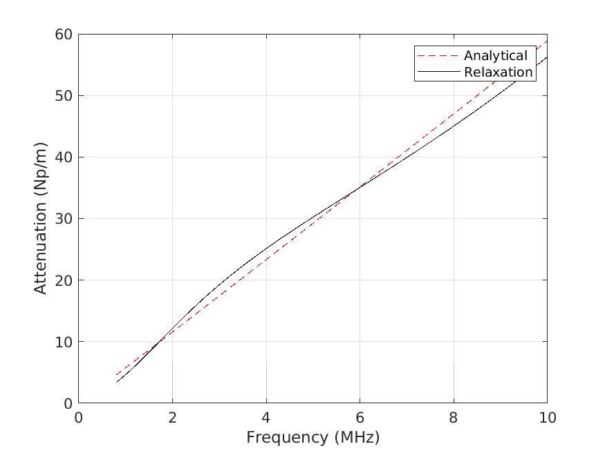
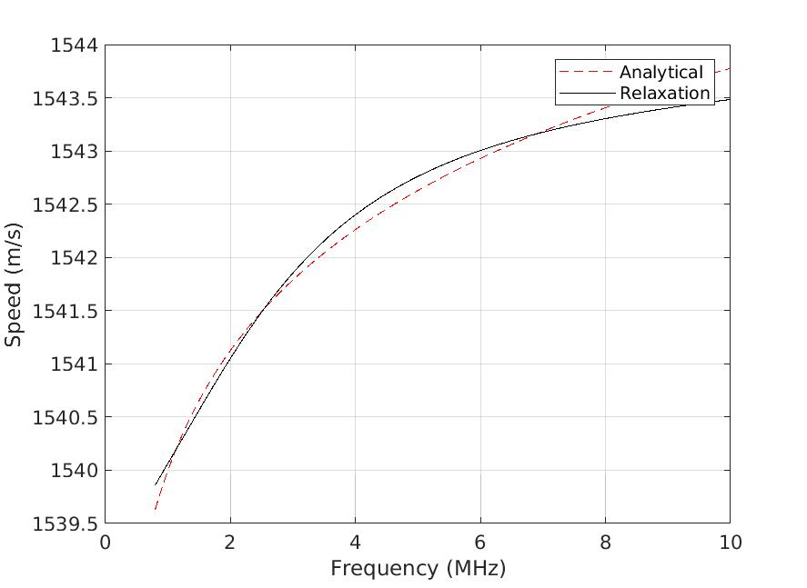
Figure 1: Validation of numerical attenuation/dispersion comparing analytical solution for an attenuation law that is linearly dependent on frequency (left) and its associated dispersion curve calculated from the Kramers Kronig relation (right).

A convolutional perfectly matched layer was implemented as described above with a cubic increase in the attenuation constant. The dispersion relation in the PML was kept constant relative to the interior of the domain to minimize any impedance discontinuoities. This is a key advantage of describing PMLs with relaxation mechanisms. The reflection coefficient, measured in dB as the amplitude of the reflected wave for normal incidence is shown in Fig. 2 (left) for different boundary layer thicknesses and in Fig. 2 (right) for different grid sizes.

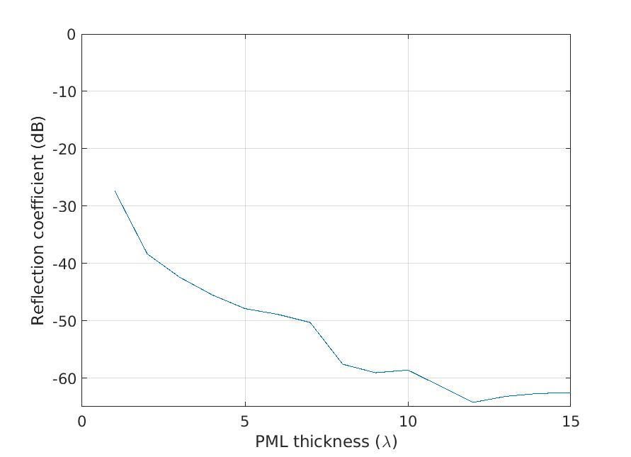
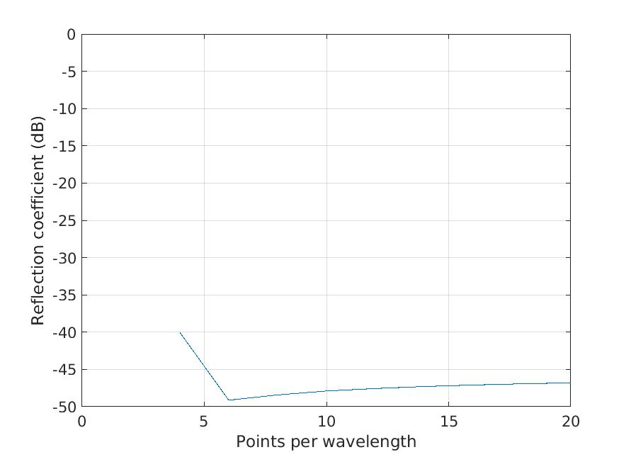
Figure 2: Validation of the perfectly matched layers, as function of boundary thickness and grid size.

A 2D plane wave was transmitted in a material with no attenuation/dispersion and compared to 1D solutions of the inviscid quadratic Burgers equation solved with a Rusanov scheme. The reference Rusanov solutions were implemented on a grid that was 10 times finer (150 points per wavelength) than the Fullwave solver (15 points per wavelength). A close matched is obtained both in the frequency (Fig. 3, left) and time domains (Fig. 3, middle and right). The frequency domain error shows that the Fullwave solution is accurate up to the 7th harmonic, indicating that the spectral support fails just before Nyquist, i.e. the fundamental sampling limit for this grid size, which occurs at 7.5 $f0$.

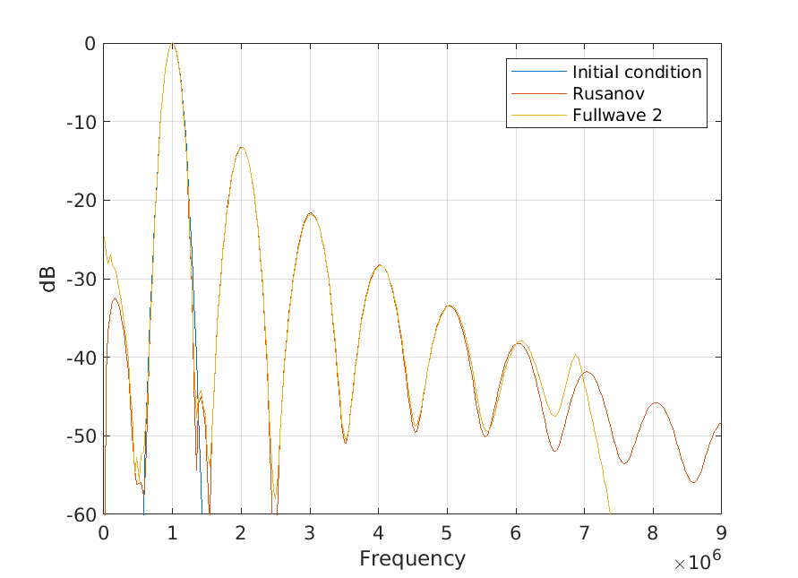
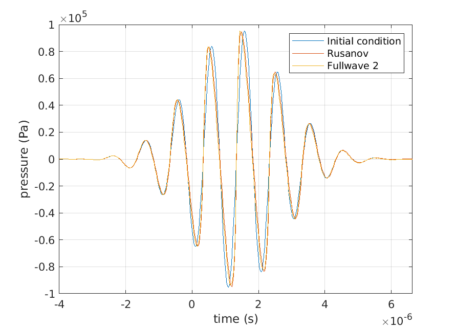
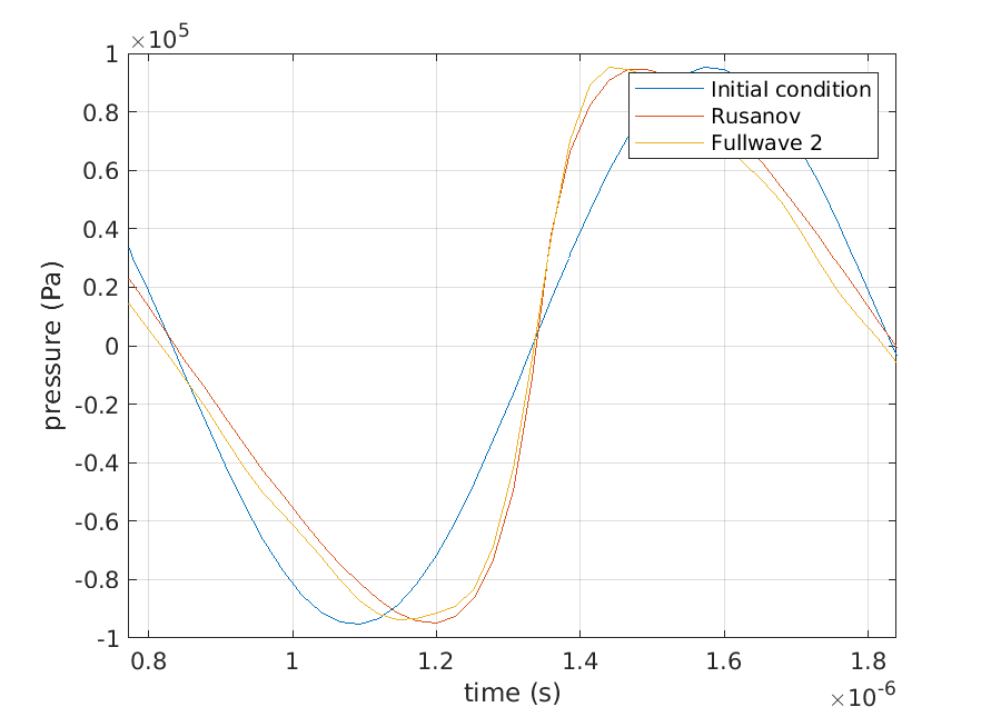
Figure 3: Comparison of nonlinearity described by Rusanov 1D solution to Burgers equation using 150 points per wavelength and Fullwave solution with a 15 points per wavelength grid. Fullwave solution is accurate up to the 7th harmonic, indicating that the spectral support fails just before Nyquist, i.e. the fundamental sampling limit for this grid size, which occurs at 7.5 $f_{0}$.

B-mode imaging simulations of a C5-2V siemens array were implemented using transmit receive simulations in the Visible Human abdomen [10, 11, 12]. To obtain this measurement and to calibrate the simulation tool, a fresh porcine liver was placed under the porcine abdomen and the same focused acquisition sequence was used to generate B-mode images experimentally. To avoid confounding effects on speckle brightness from vessels, a homogeneous vessel-free imaging view was selected and no vessels were modeled in the simulations. The average speckle brightness in the liver between 80-100 mm was measured to be -57.8 dB. The same measurement was performed in simulation with the Fullwave tool (Fig. 4). The impedance of the 35 $\mu$m sub-resolution scatterers in the liver were swept across values ranging between 0.5% to 10% and the best match was found for 4.0%. At this impedance value, the average brightness in the simulated liver was measured to be -57.5 dB. The LOC estimates, a measure of the signal to clutter/noise ratio in the channel signals [13], were found to be 0.32$\pm$0.093 in the experimental data and 0.31$\pm$0.037 in the simulated data.

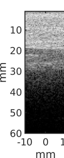
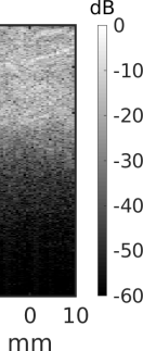
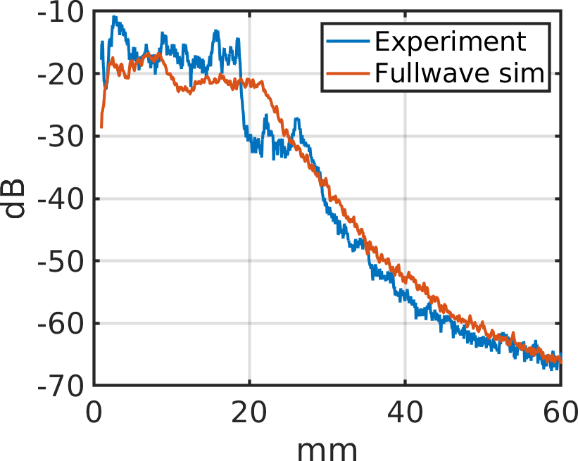
Figure 4: Experimental beamformed data from the C5-2v transducer imaging through a 20 mm pork belly sample (left). Simulated beamformed data from the C5-2v Fullwave simulation through the 2 cm human abdominal wall (middle). The average speckle brightness as a function of depth shows excellent agreement with the reverberation ringdown between experiment and simulation in the post-abdominal region beyond 20 mm depth (right).

III Summary and conclusion

A formulation of the nonlinear attenuating wave equation was developed to allow the use of high order finite differences on a staggered grid. This numerical solver was implemented and validated in terms of attenuation, nonlinearity, and ability to simulate ultrasound waves propagating in the human body. In these usage cases an excellent agreement was found. Future work will extend the validation cases.

References

- [1] J. Virieux, “Sh-wave propagation in heterogeneous media: Velocity-stress finite-difference method,” Geophysics, vol. 49, no. 11, pp. 1933–1942, 1984.
- [2] ——, “P-SV wave propagation in heterogeneous media: velocity-stress finite-difference method,” Geophysics, vol. 51, no. 4, pp. 889–901, 1986.
- [3] D. W. Zingg, “Comparison of high-accuracy finite-difference methods for linear wave propagation,” SIAM Journal on Scientific Computing, vol. 22, no. 2, pp. 476–502, 2000.
- [4] P. Moczo, J. Kristek, V. Vavrycuk, R. Archuleta, and L. Halada, “3D heterogeneous staggered-grid finite-difference modeling of seismic motion with volume harmonic and arithmetic averaging of elastic moduli and densities,” Bulletin of the Seismological Society of America, vol. 92, no. 8, pp. 3042–3066, 2002.
- [5] S. Tan and L. Huang, “An efficient finite-difference method with high-order accuracy in both time and space domains for modelling scalar-wave propagation,” Geophysical Journal International, vol. 197, no. 2, pp. 1250–1267, 2014.
- [6] X. Yuan, D. Borup, J. W. Wiskin, M. Berggren, R. Eidens, and S. A. Johnson, “Formulation and validation of berenger’s pml absorbing boundary for the fdtd simulation of acoustic scattering,” IEEE Transactions on Ultrasonics, Ferroelectrics, and Frequency Control, vol. 44, no. 4, pp. 816–822, 1997.
- [7] J. Huijssen and M. D. Verweij, “An iterative method for the computation of nonlinear, wide-angle, pulsed acoustic fields of medical diagnostic transducers,” The Journal of the Acoustical Society of America, vol. 127, no. 1, pp. 33–44, 2010.
- [8] S. Aanonsen, T. Barkve, J. N. Tjøtta, and S. Tjøtta, “Distortion and harmonic generation in the nearfield of a finite amplitude sound beam,” J. Acoust. Soc. Am., vol. 75, pp. 749–768, 1984.
- [9] M. O’Donnell, E. Jaynes, and J. Miller, “Kramers–kronig relationship between ultrasonic attenuation and phase velocity,” The Journal of the Acoustical Society of America, vol. 69, no. 3, pp. 696–701, 1981.
- [10] V. Spitzer, M. Ackerman, A. Scherzinger, and D. Whitlock, “The visible human male: a technical report,” Journal of the American Medical Informatics Association, vol. 3, no. 2, pp. 118–130, 1996.
- [11] G. Pinton, “Ultrasound imaging of the human body with three dimensional full-wave nonlinear acoustics. part 1: simulations methods,” arXiv, 2003.06934, 2020.
- [12] ——, “Ultrasound imaging with three dimensional full-wave nonlinear acoustic simulations. part 2: sources of image degradation in intercostal imaging,” arXiv, 2003.06927, 2020.
- [13] W. Long, N. Bottenus, and G. E. Trahey, “Lag-one coherence as a metric for ultrasonic image quality,” vol. 65, no. 10, pp. 1768–1780, 2018.