Fast Calculation of Gravitational Lensing Properties of Elliptical Navarro-Frenk-White and Hernquist Density Profiles

Abstract

We present a new approach for fast calculation of gravitational lensing properties, including the lens potential, deflection angles, convergence, and shear, of elliptical Navarro-Frenk-White (NFW) and Hernquist density profiles, by approximating them by superpositions of elliptical density profiles for which simple analytic expressions of gravitational lensing properties are available. This model achieves high fractional accuracy better than $10^{-4}$ in the range of the radius normalized by the scale radius of $10^{-4}-10^{3}$. These new approximations are $\sim 300$ times faster in solving the lens equation for a point source compared with the traditional approach resorting to expensive numerical integrations, and are implemented in glafic software.

1 Introduction

Gravitational lensing provides an important means of studying the Universe. With its purely gravitational nature and well-known underlying physics, gravitational lensing can be used to measure the dark matter distribution in galaxies and clusters of galaxies as well as to probe cosmological parameters (see e.g., Bartelmann & Schneider, 2001; Treu, 2010; Kneib & Natarajan, 2011; Limousin et al., 2013; Treu & Marshall, 2016; Oguri, 2019; Umetsu, 2020, for reviews).

In many cases, information on mass distributions and cosmological parameters is extracted by comparing gravitational lensing observables with model predictions assuming parametrized models of mass distributions. One of the most popular models that are used for the analysis of gravitational lensing is the Navarro et al. (1997, hereafter NFW) profile that is a model to represent the radial density profile of dark matter halos in $N$-body simulations. On the other hand, the stellar mass distribution is often modeled by the Hernquist (1990) profile that approximates the so-called de Vaucouleurs profile for elliptical galaxies.

One of the advantages of the NFW and Hernquist profiles is that analytic expressions of their gravitational lensing properties are available under the assumption of the spherical symmetry (Bartelmann, 1996; Wright & Brainerd, 2000; Keeton, 2001a). However, observed galaxies and dark matter halos are not spherically symmetric but are more like elliptical in projection on the sky. Therefore calculations of gravitational lensing properties for elliptical density profiles are important for a range of applications of gravitational lensing. For instance, the elliptical NFW density profile has been used to measure projected ellipticities of cluster-scale dark matter halos (Evans & Bridle, 2009; Oguri et al., 2010, 2012; Umetsu et al., 2018; Okabe et al., 2020) and to confirm an important prediction of the standard cold dark matter model.

A challenge of the gravitational lensing analysis using elliptical density profiles lies in the fact that analytic expressions of their gravitational lensing properties are available only for a very limited number of mass models. For instance, analytic expressions for elliptical NFW and Hernquist density profiles are not known, and as a result one has to resort to numerical integrations, which are computationally expensive, to derive their gravitational lensing properties (Schramm, 1990; Keeton, 2001a).

There are several possible ways to overcome such difficulty, at least partly. Golse & Kneib (2002) consider the elliptical NFW potential, in which the ellipticity is introduced in isopotential contours rather than in isodensity contours (see also Meneghetti et al., 2003). While this model enables fully analytic calculations of gravitational lensing properties, is also used for measuring projected ellipticities of cluster-scale dark matter halos (e.g., Richard et al., 2010), and is widely implemented in strong lens modeling softwares including gravlens (Keeton, 2001b, 2010), lenstool (Jullo et al., 2007), glafic (Oguri, 2010), and lenstronomy (Birrer & Amara, 2018), it predicts unphysical density distributions (e.g., dumbbell-like isodensity contours and negative densities) when the ellipticity is large. Du et al. (2020) propose a broken power-law model, which can resemble the NFW and Hernquist profiles, as an analytically tractable elliptical lens model (see also Barkana, 1998; Tessore & Metcalf, 2015). Methods using Fourier series are also explored in Schneider & Weiss (1991) and Chae (2002).

In this paper, we propose models that approximate elliptical NFW and Hernquist density profiles and have analytic expressions for their gravitational lensing potentials, deflection angles, convergence and shear. This is done by expressing NFW and Hernquist profiles by superpositions of models with known analytic expressions. The idea to describe a distribution by a superposition of analytically tractable models itself is not new. For instance, Hogg & Lang (2013) model two-dimensional images of galaxies by mixtures of Gaussians for fast pixel rendering and fast convolution with the telescope point-spread function. Baltz et al. (2009) propose to compute gravitational lensing properties of elliptical density models by a superposition of elliptical potential models with different ellipticities. Shajib (2019) explore a method to compute lensing and kinematic properties of arbitrary elliptical mass models by a superposition of elliptical Gaussian density profiles. Our work is similar in spirit by that of Shajib (2019) but proposes to use a different basis function whose analytic expression of gravitational lensing properties is simple and easy to implement in codes.

2 Elliptical NFW and Hernquist Density Profiles

2.1 General Elliptical Mass Model

First, we consider a family of spherically symmetric density profiles with a characteristic scale $r_{0}$

$$\rho(\boldsymbol{x})=\rho_{0}\,f\left(\frac{|\boldsymbol{x}|}{r_{0}}\right).$$ (1)

The corresponding convergence is also a circular symmetric and is written as

$$\kappa(r)=\frac{\rho_{0}}{\Sigma_{\rm cr}}\int_{-\infty}^{\infty}dz\,f\left(\frac{\sqrt{r^{2}+z^{2}}}{r_{0}}\right)=\frac{\rho_{0}r_{0}}{\Sigma_{\rm cr}}\kappa_{\rm dl}\left(\frac{r}{r_{0}}\right),$$ (2)

where $\Sigma_{\rm cr}$ is a critical surface mass density. We consider an elliptical mass model for which isodensity contours of convergence have an elliptical symmetry. Specifically, the ellipticity is introduced by replacing $r$ in Equation (2) to $v$ as

$$r\rightarrow v=\sqrt{qx^{2}+\frac{y^{2}}{q}},$$ (3)

where $q$ is the axis ratio of isodensity contours. Defining $b_{\rm norm}=\rho_{0}r_{0}/\Sigma_{\rm cr}$, convergence reduces to

$$\kappa(x,y)=b_{\rm norm}\kappa_{\rm dl}\left(\frac{\xi}{r_{0}^{\prime}}\right),$$ (4)

where

$$\xi=\sqrt{x^{2}+\frac{y^{2}}{q^{2}}},$$ (5)

$$r_{0}^{\prime}=\frac{r_{0}}{\sqrt{q}}.$$ (6)

Gravitational lensing properties of this elliptical model can be computed by one-dimensional numerical integrations (Schramm, 1990; Keeton, 2001a).

2.2 NFW Profile

The three-dimensional NFW radial density profile is given by (Navarro et al., 1997)

$$\rho^{\rm NFW}(r)=\frac{\rho_{\rm s}}{(r/r_{\rm s})(1+r/r_{\rm s})^{2}},$$ (7)

where $\rho_{\rm s}$ is the characteristic density and $r_{\rm s}$ is the scale radius. Choosing $\rho_{0}=4\rho_{s}$ and $r_{0}=r_{\rm s}$, we obtain (Bartelmann, 1996)

$$\kappa_{\rm dl}^{\rm NFW}(u)=\frac{1}{2(u^{2}-1)}\left[1-F(u)\right],$$ (8)

where $F(u)$ is defined by

$$F(u)=\begin{cases}{\displaystyle\frac{1}{\sqrt{1-u^{2}}}{\rm arctanh}\sqrt{1-u^{2}}}&{\displaystyle(u<1)},\\ {\displaystyle\frac{1}{\sqrt{u^{2}-1}}\arctan\sqrt{u^{2}-1}}&{\displaystyle(u>1)}.\end{cases}$$ (9)

2.3 Hernquist Profile

The three-dimensional Hernquist radial density profile is given by (Hernquist, 1990)

$$\rho^{\rm Hern}(r)=\frac{M}{2\pi(r/r_{\rm b})(1+r/r_{\rm b})^{3}},$$ (10)

where $M$ is the total mass and $r_{\rm b}$ is is the scale and is known to be related with the half-mass radius $R_{\rm e}$ of the project surface mass density as $r_{\rm b}=0.551R_{\rm e}$. Choosing $\rho_{0}=M/(2\pi r_{\rm b}^{3})$ and $r_{0}=r_{\rm b}$, we obtain (Keeton, 2001a)

$$\kappa_{\rm dl}^{\rm Hern}(u)=\frac{1}{(u^{2}-1)^{2}}\left[-3+(2+u^{2})F(u)\right],$$ (11)

where $F(u)$ is defined in Equation (9).

3 Approximating NFW and Hernquist Profiles

3.1 Cored Steep Ellipsoid as a Basis Function

In this paper, we propose to approximate $\kappa_{\rm dl}^{\rm NFW}(u)$ (equation 8) and $\kappa_{\rm dl}^{\rm Hern}(u)$ (equation 10) as

$$\kappa_{\rm dl}^{\rm NFW}(u)\approx\sum_{i=1}^{N_{\rm NFW}}A^{\rm NFW}_{i}\kappa^{\rm CSE}_{\rm dl}(u;S^{\rm NFW}_{i}),$$ (12)

$$\kappa_{\rm dl}^{\rm Hern}(u)\approx\sum_{i=1}^{N_{\rm Hern}}A^{\rm Hern}_{i}\kappa^{\rm CSE}_{\rm dl}(u;S^{\rm Hern}_{i}),$$ (13)

where $\kappa_{\rm dl}^{\rm CSE}(u)$ has the following functional form

$$\kappa^{\rm CSE}_{\rm dl}(u;s)=\frac{1}{2(s^{2}+u^{2})^{3/2}},$$ (14)

which is an unnamed density profile studied by Keeton & Kochanek (1998) and Keeton (2001a). For the sake of convenience, in what follows we call (the elliptical extension of) this model as a cored steep ellipsoid (CSE).

Once the above approximations are derived, approximated gravitational lensing properties of the elliptical NFW and Hernquist density profiles are fully analytically tractable because analytic expressions of gravitational lensing properties of the CSE profile are available, as explicitly shown in Section 3.2.

We point out that the use of the CSE profile has several advantages over the elliptical Gaussian profile used in Shajib (2019). One is that first and second derivatives of the lens potential, which are main quantities used for solving the lens equation and fitting observed strong lens systems, are described by simple algebraic functions and hence can be computed very efficiently in codes, in contrast to those for the elliptical Gaussian for which analytic expressions involve special functions that are computationally expensive. Second, unlike the elliptical Gaussian case, a simple analytic expression of the lens potential is also available for the CSE profile. Third, since the CSE model is less localized than the elliptical Gaussian model, it is expected that we need a smaller number of CSE components to fit the NFW and Hernquist profiles.

3.2 Gravitational Lensing Properties of Cored Steep Ellipsoid

Here we give explicit expressions of the lens potential as well as first and second derivatives of the lens potential for the CSE model, which are originally derived in Keeton & Kochanek (1998). Specifically, we consider an elliptical density profile of the following form

$$\kappa^{\rm CSE}(x,y)=\kappa^{\rm CSE}_{\rm dl}(\xi;s)=\frac{1}{2(s^{2}+\xi^{2})^{3/2}},$$ (15)

where $\xi$ is defined in Equation (5). The corresponding lens potential is given by

$$\phi^{\rm CSE}(x,y)=\frac{q}{2s}\ln\Psi-\frac{q}{s}\ln\left[(1+q)s\right],$$ (16)

where $\Psi$ denotes

$$\Psi=(\psi+s)^{2}+(1-q^{2})x^{2},$$ (17)

$$\psi=\sqrt{q^{2}(s^{2}+x^{2})+y^{2}}.$$ (18)

We note that the second term of the right hand side of Equation (16) is constant and hence can be omitted. First and second derivatives of the lens potential are simply given by

$$\phi_{x}^{\rm CSE}(x,y)=\frac{qx(\psi+q^{2}s)}{s\psi\Psi},$$ (19)

$$\phi_{y}^{\rm CSE}(x,y)=\frac{qy(\psi+s)}{s\psi\Psi},$$ (20)

$$\phi_{xx}^{\rm CSE}(x,y)=\frac{q}{s\Psi}\left[1+\frac{q^{2}s(q^{2}s^{2}+y^{2})}{\psi^{3}}-\frac{2x^{2}(\psi+q^{2}s)^{2}}{\psi^{2}\Psi}\right],$$ (21)

$$\phi_{yy}^{\rm CSE}(x,y)=\frac{q}{s\Psi}\left[1+\frac{q^{2}s(s^{2}+x^{2})}{\psi^{3}}-\frac{2y^{2}(\psi+s)^{2}}{\psi^{2}\Psi}\right],$$ (22)

$$\phi_{xy}^{\rm CSE}(x,y)=-\frac{qxy}{s\Psi}\left[\frac{q^{2}s}{\psi^{3}}+\frac{2(\psi+q^{2}s)(\psi+s)}{\psi^{2}\Psi}\right].$$ (23)

Given these analytic expressions, we can easily derive approximated gravitational lensing properties of the elliptical NFW and Hernquist density profiles. For instance, the first $x$-derivative (deflection angle) of the lens potential of the elliptical NFW density profile is approximated as

$$\phi_{x}^{\rm NFW}(x,y)\approx r_{0}^{\prime}b_{\rm norm}\sum_{i=1}^{N_{\rm NFW}}A^{\rm NFW}_{i}\phi^{\rm CSE}_{x}\left(\frac{x}{r_{0}^{\prime}},\frac{y}{r_{0}^{\prime}};S^{\rm NFW}_{i}\right),$$ (24)

and other approximated lensing properties can also be obtained in a similar manner.

Table 1: Parameters for the NFW profile.

$i$	$A_{i}^{\rm NFW}$	$S_{i}^{\rm NFW}$
1	1.648988e-18	1.082411e-06
2	6.274458e-16	8.786566e-06
3	3.646620e-17	3.292868e-06
4	3.459206e-15	1.860019e-05
5	2.457389e-14	3.274231e-05
6	1.059319e-13	6.232485e-05
7	4.211597e-13	9.256333e-05
8	1.142832e-12	1.546762e-04
9	4.391215e-12	2.097321e-04
10	1.556500e-11	3.391140e-04
11	6.951271e-11	5.178790e-04
12	3.147466e-10	8.636736e-04
13	1.379109e-09	1.405152e-03
14	3.829778e-09	2.193855e-03
15	1.384858e-08	3.179572e-03
16	5.370951e-08	4.970987e-03
17	1.804384e-07	7.631970e-03
18	5.788608e-07	1.119413e-02
19	3.205256e-06	1.827267e-02
20	1.102422e-05	2.945251e-02
21	4.093971e-05	4.562723e-02
22	1.282206e-04	6.782509e-02
23	4.575541e-04	1.596987e-01
24	7.995270e-04	1.127751e-01
25	5.013701e-03	2.169469e-01
26	1.403508e-02	3.423835e-01
27	5.230727e-02	5.194527e-01
28	1.898907e-01	8.623185e-01
29	3.643448e-01	1.382737e+00
30	7.203734e-01	2.034929e+00
31	1.717667e+00	3.402979e+00
32	2.217566e+00	5.594276e+00
33	3.187447e+00	8.052345e+00
34	8.194898e+00	1.349045e+01
35	1.765210e+01	2.603825e+01
36	1.974319e+01	4.736823e+01
37	2.783688e+01	6.559320e+01
38	4.482311e+01	1.087932e+02
39	5.598897e+01	1.477673e+02
40	1.426485e+02	2.495341e+02
41	2.279833e+02	4.305999e+02
42	5.401335e+02	7.760206e+02
43	9.743682e+02	2.143057e+03
44	1.775124e+03	1.935749e+03

Table 2: Parameters for the Hernquist profile.

$i$	$A_{i}^{\rm Hern}$	$S_{i}^{\rm Hern}$
1	9.200445e-18	1.199110e-06
2	2.184724e-16	3.751762e-06
3	3.548079e-15	9.927207e-06
4	2.823716e-14	2.206076e-05
5	1.091876e-13	3.781528e-05
6	6.998697e-13	6.659808e-05
7	3.142264e-12	1.154366e-04
8	1.457280e-11	1.924150e-04
9	4.472783e-11	3.040440e-04
10	2.042079e-10	4.683051e-04
11	8.708137e-10	7.745084e-04
12	2.423649e-09	1.175953e-03
13	7.353440e-09	1.675459e-03
14	5.470738e-08	2.801948e-03
15	2.445878e-07	9.712807e-03
16	4.541672e-07	5.469589e-03
17	3.227611e-06	1.104654e-02
18	1.110690e-05	1.893893e-02
19	3.725101e-05	2.792864e-02
20	1.056271e-04	4.152834e-02
21	6.531501e-04	6.640398e-02
22	2.121330e-03	1.107083e-01
23	8.285518e-03	1.648028e-01
24	4.084190e-02	2.839601e-01
25	5.760942e-02	4.129439e-01
26	1.788945e-01	8.239115e-01
27	2.092774e-01	6.031726e-01
28	3.697750e-01	1.145604e+00
29	3.440555e-01	1.401895e+00
30	5.792737e-01	2.512223e+00
31	2.325935e-01	2.038025e+00
32	5.227961e-01	4.644014e+00
33	3.079968e-01	9.301590e+00
34	1.633456e-01	2.039273e+01
35	7.410900e-02	4.896534e+01
36	3.123329e-02	1.252311e+02
37	1.292488e-02	3.576766e+02
38	2.156527e+00	2.579464e+04
39	1.652553e-02	2.944679e+04
40	2.314934e-02	2.834717e+03
41	3.992313e-01	5.931328e+04

4 Result

4.1 Derivation of $A_{i}$ and $S_{i}$

We determine $A_{i}$ and $S_{i}$ in Equations (12) and (13) so that these equations hold accurately. To do so, we quantify the goodness of fit by the following likelihood function

$$\mathcal{L}=\exp\left[-\frac{1}{2}\sum_{j}\frac{\left\{\kappa_{\rm dl}^{\rm X}(u_{j})-\sum_{i=1}^{N_{\rm X}}A^{\rm X}_{i}\kappa^{\rm CSE}_{\rm dl}(u_{j};S^{\rm X}_{i})\right\}^{2}}{\kappa_{\rm dl}^{\rm X}(u_{j})^{2}\sigma^{2}}\right],$$ (25)

where ${\rm X}$ denotes either ${\rm NFW}$ or ${\rm Hern}$, and we set $\sigma=10^{-4}$ that is an approximate target accuracy. To fit $\kappa_{\rm dl}(u)$ for a wide range of $u$, $u_{j}$ runs in the range $10^{-6}\leq u\leq 10^{3}$ and are equally spaced in logarithmic scale with an interval of $\Delta(\log_{10}u)=0.05$. For a given $N_{\rm X}$, we set the initial condition of $S^{\rm X}_{i}$ such that they are also equally spaced in logarithmic scale in the same $u$ range, and search the maximum likelihood combining the Metropolis–Hastings algorithm with several different random seeds and the downhill simplex method. We repeat this procedure as a function of $N_{\rm X}$ to find an optimal $N_{\rm X}$ that balances the number with the accuracy.

Tables 1 and 2 shows the parameters $A^{\rm X}_{i}$ and $S^{\rm X}_{i}$ derived using the method mentioned above, for the NFW and Hernquist profiles, respectively. The numbers of the CSE components are $N_{\rm NFW}=44$ and $N_{\rm Hern}=41$.

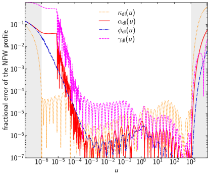
Figure 1: The fractional error of the approximation of convergence $\kappa_{\rm dl}(u)$ of the NFW profile given by Equation (12) is shown by a dotted line. The parameters $A^{\rm NFW}_{i}$ and $S^{\rm NFW}_{i}$ are summarized in Table 1. The fractional errors of the approximation of the deflection angle $\alpha_{\rm dl}(u)$ (solid), the lens potential $\phi_{\rm dl}(u)$ (dot-dashed), and shear $\gamma_{\rm dl}(u)$ (dashed) are also shown. The shaded regions indicate the ranges of $u$ that are not used for deriving the parameters $A^{\rm NFW}_{i}$ and $S^{\rm NFW}_{i}$.

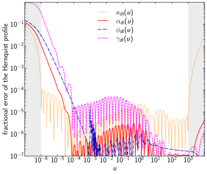
Figure 2: Same as Figure 1, but for the Hernquist profile.

4.2 Accuracy

We check the accuracy of our approximations given by Equations (12) and (13) in Figures 1 and 2, respectively. In the Figures, we check the accuracy of not only convergence $\kappa_{\rm dl}(u)$ but also the deflection angle

$$\alpha_{\rm dl}(u)=\frac{2}{u}\int_{0}^{u}u^{\prime}\kappa_{\rm dl}(u^{\prime})du^{\prime},$$ (26)

the lens potential

$$\phi_{\rm dl}(u)=2\int_{0}^{u}u^{\prime}\kappa_{\rm dl}(u^{\prime})\ln\left(\frac{u}{u^{\prime}}\right)du^{\prime},$$ (27)

and shear

$$\gamma_{\rm dl}(u)=\frac{\alpha_{\rm dl}(u)}{u}-\kappa_{\rm dl}(u),$$ (28)

as all these are important quantities that are frequently used for the gravitational lensing analysis. We find that our approximation of convergence is accurate at better than $10^{-4}$ for almost all the range used for fitting, $10^{-6}<u<10^{3}$. On the other hand, due to its non-local nature, the large deviation of convergence at $u<10^{-6}$ propagates into the deflection angle, the lens potential, and shear up to $u\sim 10^{-4}$. Hence we conclude that our approximation using the CSE is accurate at better than $10^{-4}$ for all these lensing properties in the range of the radius normalized by the scale radius of $10^{-4}-10^{3}$, both for the NFW and Hernquist profiles.

In some cases, accuracy requirements are less strict due to e.g., large measurement uncertainties in observations. Our procedure given in Section 4.1 in fact allows us to construct models with the lower accuracy using the smaller number the CSE components. As a specific example, we find that it is possible to construct models that achieve the accuracy better than $10^{-2}$ in the same range of the radius normalized by the scale radius of $10^{-4}-10^{3}$ using the $N_{\rm NFW}=16$ and $N_{\rm Hern}=13$ CSE components. The parameters $A^{\rm X}_{i}$ and $S^{\rm X}_{i}$ for this lower accuracy case are shown in Tables 3 and 4.

Table 3: Parameters for the NFW profile for the lower accuracy case.

$i$	$A_{i}^{\rm NFW}$	$S_{i}^{\rm NFW}$
1	1.434960e-16	4.041628e-06
2	5.232413e-14	3.086267e-05
3	2.666660e-12	1.298542e-04
4	7.961761e-11	4.131977e-04
5	2.306895e-09	1.271373e-03
6	6.742968e-08	3.912641e-03
7	1.991691e-06	1.208331e-02
8	5.904388e-05	3.740521e-02
9	1.693069e-03	1.153247e-01
10	4.039850e-02	3.472038e-01
11	5.665072e-01	1.017550e+00
12	3.683242e+00	3.253031e+00
13	1.582481e+01	1.190315e+01
14	6.340984e+01	4.627701e+01
15	2.576763e+02	1.842613e+02
16	1.422619e+03	8.206569e+02

Table 4: Parameters for the Hernquist profile for the lower accuracy case.

$i$	$A_{i}^{\rm Hern}$	$S_{i}^{\rm Hern}$
1	7.775712e-16	4.426947e-06
2	3.279878e-13	3.551219e-05
3	2.374931e-11	1.639271e-04
4	1.137151e-09	6.047024e-04
5	5.314908e-08	2.180958e-03
6	2.466940e-06	7.843573e-03
7	1.125917e-04	2.809420e-02
8	4.700637e-03	9.893403e-02
9	1.257748e-01	3.246017e-01
10	9.744152e-01	9.409923e-01
11	1.434502e+00	2.929948e+00
12	5.548243e-01	1.545137e+01
13	6.123431e-01	1.883671e+03

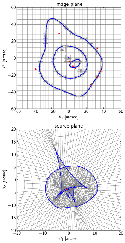
Figure 3: Critical curves and caustics of an example of the multiple lens plane mass model that is used to check the performance of the approximation are shown by solid lines. In this example three elliptical NFW and three elliptical Hernquist lenses placed over three lens planes at $z=0.3$, $0.6$, and $0.9$ are included in total. Filled triangles show the position of a point source at $z=3$ in the source plane as well as positions of the corresponding multiple images in the image plane. Adaptive mesh that is prepared in solving the lens equation with glafic software (Oguri, 2010) is also shown by gray lines.

4.3 Demonstration with glafic

The new approximations (the higher accuracy version with $N_{\rm NFW}=44$ and $N_{\rm Hern}=41$) of the elliptical NFW and Hernquist density profiles proposed in this paper are implemented in glafic software (Oguri, 2010) as lens model names of anfw and ahern, respectively. The latest version of glafic also supports multiple lens plane gravitational lensing (e.g., Schneider et al., 1992). Adopting three lens plane gravitational lensing as an example, we explicitly check how our new approximations speed up gravitational lensing calculations.

In our specific example, we consider three lens planes at redshift $z=0.3$, $0.6$, and $0.9$. At each lens plane, we place a compound lens comprising the elliptical NFW and Hernquist profiles with masses of $3\times 10^{14}h^{-1}M_{\odot}$ and $3\times 10^{12}h^{-1}M_{\odot}$, respectively. All these NFW and Hernquesit components have non-zero ellipticties $1-q$ ranging from $0.2$ to $0.8$. We derive multiple images of a point source placed at redshift $z=3$ with glafic. When solving the lens equation, the initial grid is set with a spacing of $3^{\prime\prime}$ (pix_poi $=3.0$) and the grid size is adaptively refined up to fifth level (maxlev $=5$).

Figure 3 shows critical curves, caustics, and positions of multiple images in this example. We find that shapes of the critical curve and caustic are almost indistinguishable between results with and without the approximation. In this specific example, there are 9 multiple images, and their positions and magnifications with and without the approximation match typically within $0.02^{\prime\prime}$ and $0.5\%$, respectively. These differences are sufficiently small compared with the typical accuracy of cluster mass modeling and hence are unimportant. We note that the differences in fact largely come from the imperfect accuracy of numerical integrations of the elliptical NFW and Hernquist profiles without the approximations, as those numerical integrations are slow to converge and those in glafic are accurate only up to fractional errors of $\sim 10^{-3}-10^{-4}$ level so as not to be computationally intensive.

More importantly, the new approximations make these calculations much faster. With a single core calculation with 2.3 GHz Intel Core i7, the new approximations allow us to find those multiple images in 0.13 seconds, while the calculations resorting to numerical integrations take 36 seconds to find those multiple images. Therefore, the new approximations are $\sim 300$ times faster than the traditional calculation involving numerical integrations, at least for the case of this specific example to solve the lens equation.

5 Summary

We have presented a new approach for fast calculation of gravitational lensing properties of the elliptical NFW and Hernquist density profiles. In this approach, the elliptical NFW and Hernquist density profiles are approximated by superpositions of the cored steep ellipsoid for which simple analytic expressions of gravitational lensing properties are available. These new approximations enable us to compute gravitational lensing potential, deflection angles, convergence, and shear at fractional accuracy better than $10^{-4}$ in the range of the radius normalized by the scale radius of $10^{-4}-10^{3}$, which is sufficiently wide for most of applications in both strong and weak gravitational lensing. These new approximations are also $\sim 300$ times faster in solving the lens equation for a point source compared with the traditional approach involving numerical integrations. These approximated models are already implemented in glafic software (Oguri, 2010) and are available for immediate applications.

We note that our approach enables fast calculation of lens potentials for the elliptical NFW and Hernquist density profiles, which may become important when we study the wave optics effect for which the Kirchhoff diffraction integral involving the lens potential needs to be evaluated (see e.g., Oguri, 2019, for a review).

References

- Baltz et al. (2009) Baltz, E. A., Marshall, P., & Oguri, M. 2009, J. Cosmology Astropart. Phys, 2009, 015, doi: 10.1088/1475-7516/2009/01/015
- Barkana (1998) Barkana, R. 1998, ApJ, 502, 531, doi: 10.1086/305950
- Bartelmann (1996) Bartelmann, M. 1996, A&A, 313, 697. https://arxiv.org/abs/astro-ph/9602053
- Bartelmann & Schneider (2001) Bartelmann, M., & Schneider, P. 2001, Phys. Rep., 340, 291, doi: 10.1016/S0370-1573(00)00082-X
- Birrer & Amara (2018) Birrer, S., & Amara, A. 2018, Physics of the Dark Universe, 22, 189, doi: 10.1016/j.dark.2018.11.002
- Chae (2002) Chae, K.-H. 2002, ApJ, 568, 500, doi: 10.1086/339164
- Du et al. (2020) Du, W., Zhao, G.-B., Fan, Z., et al. 2020, ApJ, 892, 62, doi: 10.3847/1538-4357/ab7a15
- Evans & Bridle (2009) Evans, A. K. D., & Bridle, S. 2009, ApJ, 695, 1446, doi: 10.1088/0004-637X/695/2/1446
- Golse & Kneib (2002) Golse, G., & Kneib, J. P. 2002, A&A, 390, 821, doi: 10.1051/0004-6361:20020639
- Hernquist (1990) Hernquist, L. 1990, ApJ, 356, 359, doi: 10.1086/168845
- Hogg & Lang (2013) Hogg, D. W., & Lang, D. 2013, PASP, 125, 719, doi: 10.1086/671228
- Jullo et al. (2007) Jullo, E., Kneib, J. P., Limousin, M., et al. 2007, New Journal of Physics, 9, 447, doi: 10.1088/1367-2630/9/12/447
- Keeton (2001a) Keeton, C. R. 2001a, arXiv e-prints, astro. https://arxiv.org/abs/astro-ph/0102341
- Keeton (2001b) —. 2001b, arXiv e-prints, astro. https://arxiv.org/abs/astro-ph/0102340
- Keeton (2010) —. 2010, General Relativity and Gravitation, 42, 2151, doi: 10.1007/s10714-010-1041-1
- Keeton & Kochanek (1998) Keeton, C. R., & Kochanek, C. S. 1998, ApJ, 495, 157, doi: 10.1086/305272
- Kneib & Natarajan (2011) Kneib, J.-P., & Natarajan, P. 2011, A&A Rev., 19, 47, doi: 10.1007/s00159-011-0047-3
- Limousin et al. (2013) Limousin, M., Morandi, A., Sereno, M., et al. 2013, Space Sci. Rev., 177, 155, doi: 10.1007/s11214-013-9980-y
- Meneghetti et al. (2003) Meneghetti, M., Bartelmann, M., & Moscardini, L. 2003, MNRAS, 340, 105, doi: 10.1046/j.1365-8711.2003.06276.x
- Navarro et al. (1997) Navarro, J. F., Frenk, C. S., & White, S. D. M. 1997, ApJ, 490, 493, doi: 10.1086/304888
- Oguri (2010) Oguri, M. 2010, PASJ, 62, 1017, doi: 10.1093/pasj/62.4.1017
- Oguri (2019) —. 2019, Reports on Progress in Physics, 82, 126901, doi: 10.1088/1361-6633/ab4fc5
- Oguri et al. (2012) Oguri, M., Bayliss, M. B., Dahle, H., et al. 2012, MNRAS, 420, 3213, doi: 10.1111/j.1365-2966.2011.20248.x
- Oguri et al. (2010) Oguri, M., Takada, M., Okabe, N., & Smith, G. P. 2010, MNRAS, 405, 2215, doi: 10.1111/j.1365-2966.2010.16622.x
- Okabe et al. (2020) Okabe, T., Oguri, M., Peirani, S., et al. 2020, MNRAS, 496, 2591, doi: 10.1093/mnras/staa1479
- Richard et al. (2010) Richard, J., Smith, G. P., Kneib, J.-P., et al. 2010, MNRAS, 404, 325, doi: 10.1111/j.1365-2966.2009.16274.x
- Schneider et al. (1992) Schneider, P., Ehlers, J., & Falco, E. E. 1992, Gravitational Lenses, doi: 10.1007/978-3-662-03758-4
- Schneider & Weiss (1991) Schneider, P., & Weiss, A. 1991, A&A, 247, 269
- Schramm (1990) Schramm, T. 1990, A&A, 231, 19
- Shajib (2019) Shajib, A. J. 2019, MNRAS, 488, 1387, doi: 10.1093/mnras/stz1796
- Tessore & Metcalf (2015) Tessore, N., & Metcalf, R. B. 2015, A&A, 580, A79, doi: 10.1051/0004-6361/201526773
- Treu (2010) Treu, T. 2010, ARA&A, 48, 87, doi: 10.1146/annurev-astro-081309-130924
- Treu & Marshall (2016) Treu, T., & Marshall, P. J. 2016, A&A Rev., 24, 11, doi: 10.1007/s00159-016-0096-8
- Umetsu (2020) Umetsu, K. 2020, A&A Rev., 28, 7, doi: 10.1007/s00159-020-00129-w
- Umetsu et al. (2018) Umetsu, K., Sereno, M., Tam, S.-I., et al. 2018, ApJ, 860, 104, doi: 10.3847/1538-4357/aac3d9
- Wright & Brainerd (2000) Wright, C. O., & Brainerd, T. G. 2000, ApJ, 534, 34, doi: 10.1086/308744