Querying in the Age of Graph Databases and Knowledge Graphs

Abstract.

Graphs have become the best way we know of representing knowledge. The computing community has investigated and developed the support for managing graphs by means of digital technology. Graph databases and knowledge graphs surface as the most successful solutions to this program. The goal of this document is to provide a conceptual map of the data management tasks underlying these developments, paying particular attention to data models and query languages for graphs.

1. Introduction

What does it mean to query a graph? What does it mean querying graph models? Any answers to these questions should try to understand the role of graphs as a conceptual tool to model data, information and knowledge. Graphs have a long tradition as medium of representation, and an impressive wide range of uses. Let us recall some highlights related to our area: underlying data structures (the hierarchical and networks database systems of the sixties (Stonebraker and Hellerstein, 2005)); semantic networks; graph neural networks; entity relationship model; XML; graph databases; the Web as universal network of information (and later of data and knowledge); and knowledge graphs. This non-exhaustive list indicates at least that some reflection is necessary before addressing the goal of this document.

Following usual practices, we performed an initial examination of what is being researched disciplinary in the area of data, graphs and knowledge. We explored five of the most salient keywords that today represent research around this area: “graph database”; “RDF”; “SPARQL”; “property graph”, “knowledge graph”, by analyzing papers in computer science (those indexed by DBLP) having these strings in their titles. Figure 1 shows the evolution of the number of publications of papers with these keyword in the title from 2010 to 2020.

In this preliminary exploration we can observe the following. The growth of “knowledge graph” papers can be seen starting in 2013, which correlates with the year after the Google’s Knowledge Graph announcement. The amount of publications about “RDF” and “SPARQL” continue to be stable. However we observe a decline when compared to “knowledge graph”. In 2015, 70% of knowledge graphs papers were about RDF/SPARQL, while that went down to 14% in 2020. Papers about “graph database” are comparatively small and there is no significant growth, while papers about “property graph” are negligible. The main takeaway message from this seems to be that publications about knowledge graphs are significantly increasing and in some sense “dominate” the area. Thus, when addressing graphs as a model for data to knowledge, we cannot ignore the obvious knowledge graph hype.

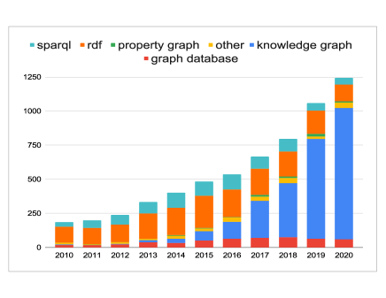
Figure 1. Number of knowledge graph related publications. Source: DBLP.

This poses the question: What are knowledge graphs and what is their relation to graph databases? In addressing this question we should be cautions about two extremes: On one hand, as Jeffrey Ullman wrote, avoid to get “engaged in hand-wringing over the idea that we [the database discipline] are becoming irrelevant” (Ullman, 2020). On the other hand, try to understand if there is someting really new under this new hype about knowledge graphs. Our preliminary hypothesis –one that we will follow here– is that this rather vague notion with no clear borders (see e.g. Appendix A in (Hogan et al., 2020)) encompasses a great variety of methods and practices dealing with data, information and knowledge, orbiting around the gravitation center of graph models.

Our intention in this brief overview is to try to convey a rough cartography of what is means to query in this new scenario, and instill in the audience some doubts and reflections we have about the development of our area as a whole. We feel that this reflection is more important than ever today, when big data, deep learning and other trends of the beginning of the 21st century have shaken computing as we know it.

1.1. A conceptual map of this document

The motivating questions for this work are why the rise of graph databases and knowledge graphs? and what are new techniques and challenges behind this boom? To try to give answers to these questions, we start by establishing in Section 2 a general picture of the area in order to better organize the conceptual map of the wide diversity of existing methods and techniques.

Then we continue by focusing on providing in Section 3 a unified and simple view of the data models behind graph databases and knowledge graphs, and show some recently established results on querying such graphs in Section 4. In particular, we focus on this latter section on queries about the local structure of a graph, the connections in it, and its global structure. Obviously, these are just a few tasks among many other relevant ones for graph databases and knowledge graphs: integration of different sources, graph data management, visualization of results, development of visual query languages, completion and refinement of graphs, search and exploration, reasoning in the presence of ontologies, different aspects related to natural language processing, analytics and the fundamental role of humans in all these challenges. The reader should bear in mind that in this document, these topics are not covered with the same level of detail as data models and querying.

2. Databases, Graphs and Knowledge Graphs

Before going to technicalities, we will present a conceptual overview of the main notions of the area and how they interplay. Our goal is to contribute to a necessary discussion of the reasons why graphs have become so prominent in data and knowledge management.

2.1. A necessary digression

Data, information and knowledge appear so often in the literature, and with so many senses, that we consider necessary to state how we understand them. These concepts predate computer science, and there is a wide and rich literature about them (Furner, 2016; Floridi, 2011; Machlup, 1981; Burke, 2015).

The notion of data has at least three main senses that play a role in our discussion. (a) A minimal unit of distinction. This lead to the notion of bit, that that can be implemented through electromagnetic media, and has many properties that makes it flexible enough for storing, transmitting and manipulating. (b) A register of aspects of reality. For example, the output of an instrument in a scientific experiment that captures some facets of “reality”. (c) A mark that leaves a phenomenon of the world. For example, the footprint (now in a stone) of a dinosaur in an archaeological site, or today’s registers from a sensor or a camera.

These three senses have something in common: data without further processing does not make much sense for humans, but it works as support for meaning and knowledge. Data in the computer science sense is this raw material in the digital format, incarnated as bits. It is important to mention then that the form how data is organized, e.g. the format and model for it, has to do essentially with the interpretation of registers in the modes of (b) and (c).

Knowledge, as understood e.g. in “knowledge representation”, “knowledge base” or “knowledge graph”, is a notion coming from the tradition of (formal) reasoning, and encompasses both, objects that statically represent knowledge (books, maps,charts, theorems, scientific laws, etc.), and mechanisms to dynamically obtain, deduce, or infer new knowledge from known premises or inputs (deductive systems, reasoners, neural networks, etc.). In fact, it is developed in (Gutiérrez and Sequeda, 2021) the idea that a great part of the developments in data and knowledge since the 50s can be thought of as a way of giving digital support to the representations (e.g. tables, graphs, etc.) and mechanisms of traditional reasoning (e.g. reasoners, expert systems, etc.).

Finally, information (which is not our concern here) speaks about semantics, meaning and interpretation for the subject that will use it. A database as such does not mean anything. It needs an interpretative apparatus, which is usually the schema and, more generally, some metadata. A digital text is a sequence of symbols. Again, needs a context, an interpretation, to get information from it. A similar phenomena occurs with a sequence of pixels: means nothing if not interpreted by a human eye or displayed by a visualization software.

2.2. Graph data and querying

Data is the raw material of our area. Databases originated in the need to store, keep safe and private, organize and operate in a efficient, reliable and permanent form, big quantities of data in computers. From these basic and essential tasks, it was developed what is probably the most important functionality of databases, namely querying, that boils down to have friendly, expressive, and efficient languages for defining, updating, transforming and extracting data. That is why query languages play such a relevant role in our discipline.

One of the landmark advances in the field was the notion of “data independence” (Codd, 1970). As computing is essentially about communicating humans and machines, or better, human knowledge and machine operation, for methodological and practical reasons one should separate the physical level (the one revolving around the machine and data) from the logical level (revolving around the way humans model reality and knowledge). Our working hypothesis is that graphs are an appropriate way of representing, both, data and knowledge. And this would be the reason why graphs began to be so prominent in this field of data and knowledge management.

Graphs have a simple data structure consisting of nodes and edges, which has the nice operational properties of expressing relations, presenting data in a rather holistic way (neither ordered nor sequentially), and last but not least, having a flexible structure that permits growing and shrinking (adding/deleting nodes and edges) and integration (of different graphs) in a natural way.

Over this nice data structure, floats a similarly nice group of conceptual ideas. First, entities, represented by nodes; second, connectivity, represented by edges and paths; and third, emergent (global) properties that the structure generates. Then it comes as no surprise that languages for querying graphs deal with extracting information about these three main features (we will discuss them in detail in Section 4):

1. local properties (nodes and neighborhoods), where pattern matching and its extensions play a key role, being usually approached with logical methods;

2. connectivity, where paths and more complicated structures need to be extracted, usually by means of a mixture of regular expressions and logical methods; and

3. global properties, where the entire structure of a graph is considered, and that essentially need different methods and approaches than those of (i) and (ii). Such methods are usually put under the graph analytics umbrella.

Figure 2. Three graph data models.

2.3. Some paradigmatic examples

To get a flavor of how these structures and ideas work in practice, let us briefly review three paradigmatic examples.

Semantic networks. One of the first attempt to represent knowledge in the form of graphs was the notion of Semantic Network (Richens, 1956; Quillan, 1963; Quillian, 1967). First born as a purely diagrammatic representation, soon researchers formalized those graphs to give them a formal semantics using logical methods. Graphs (called networks in this field) are used because they are historically very good objects to represent knowledge (in the static sense). Besides being a bridge to visualization of knowledge, semantic networks have the feature (shared with graphs in general) of highlighting and facilitating the discovery and representation of relationships.

Graph Databases. Classical relational databases are flexible enough to represent graphs, e.g. using a two attribute relation representing edges in a graph. Moreover, one could consider relational schemata as generalization of binary relations ($m$-ary relations). In this representation, nodes are entries and paths are constructed by successive joins. Why then do we need graph databases? There are at least two reasons: joins are expensive and thus, reasoning about paths –that are one the main motive to use graphs– becomes very costly. But furthermore, global properties are not easy to compute with classical queries based on logical methods.

So, it comes as no surprise that people have tried since the early days of databases to develop graph databases. First at the hardware level with the hierarchical and network models of the sixties; then at a more logical level in the eighties where we found the “golden era” of graph databases (Atkinson et al., 1992; Shapiro et al., 1993; Angles and Gutierrez, 2008). However, many constraints, among them the limitations of hardware and software, did not permit the popularization of these systems (Angles and Gutierrez, 2008).

Semantic Web. The Web is the first comprehensive system for representing, integrating and “producing” knowledge at big scale, whose key idea is taking advantage of the structure and features of the graph model (particularly the idea of integrating and extending knowledge and data by linking).

The Web was originally thought as a universal network, that is, nodes and edge were designed (with the notion of “Web page”) to be directly interpreted by humans. However, due to its scale, soon emerged the need to enrich the network to allow automation of functionalities. This is the origin of the Semantic Web (SW), where semantics means “understandable by machine” (Berners-Lee et al., 2001). The SW contained the two ideas that were to originate the current notion of knowledge graph: first, a graph structure to organize the data; second, a system which encodes not only information (i.e. data to be interpreted directly by humans), but it is also organized to derive new facts from the current ones, that is, deals essentially with knowledge. The feature of the underlying network devised by its creators, its universality (given by URIs (Berners-Lee et al., 1998) and the hypertext transfer protocol HTTP), became a problem for private companies and organizations as it was not “practical” due to privacy and property rights concern. Google overcame this, and develop the notion of knowledge graph as a “finite”, manageable, controlled and usually private Semantic Web. Nevertheless, the main concepts, namely, ontologies to integrate knowledge, and the Web as medium, would become almost standards.

2.4. Knowledge Graphs

The cases of Semantic Networks, Graph databases and the Semantic Web point to systems or software infrastructure in which graphs supports the representation, integration and production of knowledge. This rather fuzzy idea is what is at the core of the notion of Knowledge Graph. So we can define a Knowledge Graph as a software object (artifact) that represents (codifies), integrates and produces knowledge. In order to perform these functionalities, it relies on the model of graphs. In this regard, the notion of knowledge graph encompasses many previous developments (Fensel et al., 2020; Gutiérrez and Sequeda, 2021).

Knowledge representation is incorporated mainly through standardized languages, metadata and ontologies on one hand, and semantic networks and other non-formal language representations on the other. Lately, low-level representations like vector-labeled graphs were added. Notice that all of them use the flexibility of graphs for model representation (see Section 3).

Integration of knowledge is achieved essentially via the aforementioned features of graph extensibility and integration (assuming a good and standardized representation like ontologies). Thus a knowledge graph is capable of integrating knowledge from different sources, by linking or materializing them in one place, and in widely different formats, which include classical tabular data and files, natural language text, images, sound, video and other types of sensor data.

Finally, producing new knowledge is probably the main “added-value” as opposed to classical repositories of knowledge. Knowledge graphs have the capabilities of: deducing, e.g. by means of logical reasoners or neural networks; linking, that is, relating different pieces of knowledge beforehand isolated; learning, through new data and learning algorithms; and of course, generating new knowledge by human intervention through refined ways of querying it (see section 4). This new knowledge is not only user-oriented, but is utilized in parallel to “complete” and enrich the knowledge already present. As a clear example of this, we see the rapid development of knowledge graph embeddings (Bordes et al., 2013; Cai et al., 2018), and its use in the refinement and completion of knowledge graphs (Lin et al., 2015; Paulheim, 2017). In fact, they have even been used to enrich such knowledge by answering complex logical queries, which might need to deal with multiple unobserved nodes and edges in a graph (Hamilton et al., 2018; Ren et al., 2020).

These features make a knowledge graph a highly multifaceted software object. One of the best examples of this is Wikipedia. It is a repository that represents knowledge in the form of a large graph (implemented via Web link protocols). It organizes knowledge like a classic encyclopedia, the paradigm of knowledge source in pre-computing era. But the greatest feature of Wikipedia is its functionality of integrating knowledge from different sources (such as editors or links to other web pages) in different formats, both physical (text, images, sound, video, etc.) and in terms of semantics (different alphabets, languages, etc.). This makes it an unbounded networks of knowledge. Moreover, when coming to generation of knowledge, Wikipedia has a mechanism to “extract” or “produce” knowledge. In this case, these are the multiple interfaces, most of them human interfaces. Wikipedia is a knowledge graph oriented toward a final human user, that is, it does not (or at least was not conceived to) feed another software systems. DBpedia (Auer et al., 2007) and Wikidata (Vrandecic and Krötzsch, 2014) are derived system oriented to supply this facet.

3. Graph data models

In this section, we give a simple unifying view of the most popular graph data models, from the simplest ones used in graph databases to the models that have emerged to store, integrate and produce knowledge.

The following are two basic ingredients to define graph data models. Assume that Const is a set of constants, or strings, that can be used for different purposes, for example as node identifiers, edge identifiers, labels, property names or actual values (such as integers, real values or dates). Moreover, define a multigraph as a graph where multiple edges can connect two nodes, that is, a tuple $(N,E,\rho)$ where $N\subseteq\text{\rm{\bf Const}}$ is a set of nodes, $E\subseteq\text{\rm{\bf Const}}$ is a set of edges and $\rho:E\to N\times N$ is a function indicating the starting and ending node of each edge.

As a first data model, we consider labeled graphs, which are a popular and simple way to represent semi-structured data. Formally, a labeled graph is a tuple $\mathcal{L}=(N,E,\rho,\lambda)$ where $(N,E,\rho)$ is a multigraph and $\lambda:(N\cup E)\to\text{\rm{\bf Const}}$ is a function indicating the label of each node and edge. Such graphs have been called heterogeneous graphs in the literature (Sun et al., 2011; Hogan et al., 2020), as opposed to edge-labeled graphs where labels are only associated to edges (Angles et al., 2017). But here we prefer the simple term labeled graph to indicate that both nodes and edges are labeled. An example of such a graph storing information about people and their contacts is shown in Figure 2(a).

It is worth saying a few words about RDF (Cyganiak et al., 2014), a class of labeled graphs that is widely used in practice. A first characteristic that distinguish RDF graphs is that edges are replaced by triples, and they are not assigned identifiers. Formally, an RDF graph is a set of triples $(s,p,o)$ such that $s,p,o\in\text{\rm{\bf Const}}$, so that $(s,p,o)$ represents an edge from $s$ to $o$ with label $p$. A second important feature of RDF graphs is that Const is considered as a set of Uniform Resource Identifiers (URIs (Berners-Lee et al., 1998; Dürst and Suignard, 2005)), that can be used to identify any resource used by Web technologies. In this way, RDF graphs have a universal interpretation: if $c\in\text{\rm{\bf Const}}$ is used in two different RDF graphs, then $c$ is considered to represent the same element.

As a second model we consider property graphs, which are widely used in graph databases (Miller, 2013; Robinson et al., 2015; van Rest et al., 2016; Francis et al., 2018). Property graphs are defined as the extension of labeled graphs where nodes and edges can have values for some properties. Formally, a property graph is a tuple $\mathcal{P}=(N,E,\rho,\lambda,\sigma)$ where $(N,E,\rho,\lambda)$ is a labeled graph, and $\sigma:(N\cup E)\times\text{\rm{\bf Const}}\to\text{\rm{\bf Const}}$ is a partial function such that if $\sigma(o,p)=v$, then $v$ is said to be the value of property $p$ for object $o$. Besides, it is assumed that each node or edge in $\mathcal{P}$ has values for a finite number of properties (Miller, 2013; Angles et al., 2017, 2018). In Figure 2(b), we show an example of a property graph that extends the labeled graph in Figure 2(a), including as properties the name and age of a person, the zip code of the address for two people that live together, the date when someone rides a bus, and the date a contact between two people occurs.

As a final model, vector-labeled graphs are defined in a way that unifies the use of labels and properties, and allows to include in a simple way extra values that are necessary for message-passing graph algorithms (Kung, 1982), such as the Weisfeiler-Lehman graph isomorphism test (Weisfeiler and Leman, 1968; Grohe, 2011; Grohe and Schweitzer, 2020), and when graphs are used as input of graph neural networks (Merkwirth and Lengauer, 2005; Scarselli et al., 2009). Formally, a vector-labeled graph of dimension $d$, with $d\geq 1$, is a tuple $\mathcal{V}=(N,E,\rho,\lambda)$ where $(N,E,\rho)$ is a multigraph and $\lambda:(N\cup E)\to\text{\rm{\bf Const}}^{d}$ is a function that assigns a vector of values to each node and edge in the graph (Hogan et al., 2020), which is called a vector of features of dimension $d$. Hence, labels and properties are replaced by vectors of values from Const in vector-labeled graphs, as shown in Figure 2(c). In this figure, the string $\bot$ is used to represent the fact that a row in a vector does not have a value.

4. Querying: some new challenges and techniques

The goal of this section is to present pointers to some recently obtained results on querying graphs, and to pose some research questions related to them, that could be of interest not only for the database community, but also for other communities like artificial intelligence and computational logic. In this sense, this will be a growing section divided according to the features identified in Section 2 for graph query languages. In particular, we consider the following problems in this version:

• Local properties: we consider the old problem of extracting nodes from a graph, and present a recently established connection between graph neural networks and first-order logic with bounded resources, when such formalisms are viewed as query languages for node extraction.

• Connectivity properties: we consider the old problem of extracting paths from a graph, and show some recent approximation and uniform generation results.

• Global properties: we provide a simple application of the approximation result mentioned in the previous point to the definition and computation of centrality measures. Moreover, we consider the area of Explainable AI (Lundberg and Lee, 2017; Adadi and Berrada, 2018; Ribeiro et al., 2018) and, in particular, the problem of defining a declarative language for expressing natural model interpretation tasks. More precisely, we argue that such a problem corresponds to the definition of a query language for some global properties in a graph database.

4.1. A necessary terminology

As mentioned before, extracting nodes and paths is a fundamental task when retrieving knowledge from graphs (Angles et al., 2017; Francis et al., 2018). Regular expressions form the core of such an extraction task, so we need to fix a notation for regular expressions before going into the details of the results shown in this section. More precisely, a regular expression over a labeled graph $\mathcal{L}=(N,E,\rho,\lambda)$ is given by the following grammar:

$$\text{\it test}\ \ ::= \ \ \ \ell\ \mid\ (\neg\text{\it test})\ \mid\ (\text{\it test}\vee\text{\it test})\ \mid\ (\text{\it test}\wedge\text{\it test})$$

(1) $$r\ \ ::= \ \ \ ?\text{\it test}\ \mid\ \text{\it test}\ \mid\ \text{\it test}^{-}\ \mid\ (r+r)\ \mid\ (r/r)\ \mid\ (r^{*}),$$

where $\ell$ is a node or edge label in $\mathcal{L}$. An answer to $r$ over $\mathcal{L}$ is a path whose labels conform to $r$. Formally, such a path is a sequence $p=n_{0}e_{1}n_{1}e_{2}\cdots e_{i}n_{i}$, where $n_{0},n_{1},\ldots,n_{i}\in N$ and $e_{1},\ldots,e_{i}\in E$. Moreover, the starting and ending nodes of $p$ are defined as $\text{\it start}(p)=n_{0}$ and $\text{\it end}(p)=n_{i}$, respectively, and the concatenation of $p$ with a path $p^{\prime}=n_{i}e_{i+1}n_{i+1}e_{i+2}\cdots e_{i+j}n_{i+j}$ is defined as $\text{\it concat}(p,p^{\prime})=n_{0}e_{1}n_{1}e_{2}\cdots e_{i}n_{i}e_{i+1}n_{i+1}e_{i+2}\cdots e_{i+j}n_{i+j}$. With this terminology, the evaluation of $r$ over $\mathcal{L}$, denoted by $\llbracket r\rrbracket_{\mathcal{L}}$, is recursively defined as follows (omitting the usual interpretation for Boolean connectives $\neg$, $\vee$ and $\wedge$):

$$\llbracket?\ell\rrbracket_{\mathcal{L}} = \{n\mid n\in N\wedge\lambda(n)=\ell\}$$

$$\llbracket\ell\rrbracket_{\mathcal{L}} = \{n_{0}e_{1}n_{1}\mid\rho(e_{1})=(n_{0},n_{1})\wedge\lambda(e_{1})=\ell\}$$

$$\llbracket\ell^{-}\rrbracket_{\mathcal{L}} = \{n_{0}e_{1}n_{1}\mid\rho(e_{1})=(n_{1},n_{0})\wedge\lambda(e_{1})=\ell\}$$

$$\llbracket r_{1}+r_{2}\rrbracket_{\mathcal{L}} = \llbracket r_{1}\rrbracket_{\mathcal{L}}\cup\llbracket r_{2}\rrbracket_{\mathcal{L}}$$

$$\llbracket r_{1}/r_{2}\rrbracket_{\mathcal{L}} = \{\text{\it concat}(p_{1},p_{2})\mid p_{1}\in\llbracket r_{1}\rrbracket_{\mathcal{L}}\wedge p_{2}\in\llbracket r_{2}\rrbracket_{\mathcal{L}}\wedge$$

$$\phantom{\{\text{\it concat}(p_{1},p_{2})\mid\,}\text{\it end}(p_{1})=\text{\it start}(p_{2})\}$$

$$\llbracket r^{*}\rrbracket_{\mathcal{L}} = N\cup\llbracket r\rrbracket_{\mathcal{L}}\cup\llbracket r/r\rrbracket_{\mathcal{L}}\cup\llbracket r/r/r\rrbracket_{\mathcal{L}}\cup\cdots$$

Notice that $?\ell$ is used to test the label of a node, $\ell$ is used to follow an edge with label $\ell$, and $\ell^{-}$ is used to follow the opposite direction of an edge with label $\ell$. Besides, as an example of a test with Boolean connectives, observe that $\llbracket(\neg\ell_{1}\wedge\neg\ell_{2})^{-}\rrbracket_{\mathcal{L}}=\{n_{0}e_{1}n_{1}\mid\rho(e_{1})=(n_{1},n_{0})\wedge\lambda(e_{1})\neq\ell_{1}\wedge\lambda(e_{1})\neq\ell_{2}\}$. Hence, if $\mathcal{L}$ is the labeled graph in Figure 2(a), then

(2) $$\llbracket{\small\texttt{?person/contact/?infected}}\rrbracket_{\mathcal{L}}= \ \{n_{1}e_{4}n_{5}\},$$

$$\llbracket{\small\texttt{?person/rides/?bus/}}{\small\texttt{rides}}^{{\small\texttt{-}}}{\small\texttt{/?person}}\rrbracket_{\mathcal{L}}= \ \{n_{1}e_{2}n_{3}e_{3}n_{4},$$

$$\ \phantom{\{}n_{4}e_{3}n_{3}e_{2}n_{1},$$

$$\ \phantom{\{}n_{1}e_{2}n_{3}e_{2}n_{1},$$

$$\ \phantom{\{}n_{4}e_{3}n_{3}e_{3}n_{4}\}.$$

As property graphs are an extension of labeled graphs, the grammar in (1) can be easily expanded to consider property values:

$$\text{\it test}\ \ ::= \ \ \ \ell\ \mid\ (p=v)\ \mid\ (\neg\text{\it test})\ \mid\ (\text{\it test}\vee\text{\it test})\ \mid\ (\text{\it test}\wedge\text{\it test}).$$

In particular, $(p=v)$ is used to verify whether the value of property $p$ is $v$, with $p,v\in\text{\rm{\bf Const}}$. Formally, the evaluation of a regular expression $r$ over a property graph $\mathcal{P}=(N,E,\rho,\lambda,\sigma)$, denoted by $\llbracket r\rrbracket_{\mathcal{P}}$, is defined as for the case of labeled graphs but with three additional cases:

$$\llbracket?(p=v)\rrbracket_{\mathcal{P}} = \{n\mid n\in N\wedge\sigma(n,p)=v\}$$

$$\llbracket(p=v)\rrbracket_{\mathcal{P}} = \{n_{0}e_{1}n_{1}\mid\rho(e_{1})=(n_{0},n_{1})\wedge\sigma(e_{1},p)=v\}$$

$$\llbracket(p=v)^{-}\rrbracket_{\mathcal{P}} = \{n_{0}e_{1}n_{1}\mid\rho(e_{1})=(n_{1},n_{0})\wedge\sigma(e_{1},p)=v\}.$$

For example, we can extend regular expression (2) to indicate that the date of the contact between a person and an infected person is March 4th 2021:

(3) $${\small\texttt{?person/(contact}}\wedge{\small\texttt{(date\,=\,3/4/21))/?infected}}$$

Regular expressions for vector-labeled graphs are defined exactly in the same way. If $\mathcal{V}=(N,E,\rho,\lambda)$ is a vector-labeled graph of dimension $d$, then a regular expression over $\mathcal{V}$ is defined by modifying grammar (1) to consider the following tests:

$$\text{\it test}\ \ ::= \ \ \ (f_{i}=v)\ \mid\ (\neg\text{\it test})\ \mid\ (\text{\it test}\vee\text{\it test})\ \mid\ (\text{\it test}\wedge\text{\it test}),$$

where $i\in\{1,\ldots,d\}$ and $v\in\text{\rm{\bf Const}}$. In particular, $(f_{i}=v)$ is used to verify whether the value of the $i$-th feature is $v$, which is formally defined as follows:

$$\llbracket?(f_{i}=v)\rrbracket_{\mathcal{V}} = \{n\mid n\in N\wedge\lambda(n)_{i}=v\}$$

$$\llbracket(f_{i}=v)\rrbracket_{\mathcal{V}} = \{n_{0}e_{1}n_{1}\mid\rho(e_{1})=(n_{0},n_{1})\wedge\lambda(e_{1})_{i}=v\}$$

$$\llbracket(f_{i}=v)^{-}\rrbracket_{\mathcal{V}} = \{n_{0}e_{1}n_{1}\mid\rho(e_{1})=(n_{1},n_{0})\wedge\lambda(e_{1})_{i}=v\},$$

where $\lambda(n)_{i}$ refers to the $i$-th feature of $d$-dimensional vector $\lambda(n)$, and likewise for $\lambda(e_{1})_{i}$. Thus, for example, regular expression (3) can be rewritten as follows over the vector-labeled graph in Figure 2(c):

$${\small\texttt{?(f}}_{{\small\texttt{1}}}{\small\texttt{\,=\,person)/(f}}_{{\small\texttt{1}}}{\small\texttt{\,=\,contact}}\wedge{\small\texttt{f}}_{{\small\texttt{5}}}{\small\texttt{\,=\,3/4/21)/?(f}}_{{\small\texttt{1}}}{\small\texttt{\,=\,infected)}}.$$

4.2. Local properties

The task of matching a pattern against a graph is fundamental when extracting knowledge. In the previous section, we considered this problem for regular expressions, but such patterns can be specified in other frameworks, ranging from logic-based declarative languages (Harris and Seaborne, 2013; Barceló, 2013) to more procedural frameworks such as graph neural networks (Merkwirth and Lengauer, 2005; Scarselli et al., 2009). The goal of this part of the document is to show a recently established tight connection between these apparently different frameworks (Morris et al., 2019; Xu et al., 2019; Barceló et al., 2020a), which has interesting corollaries in terms of the use of declarative formalisms to specify patterns, versus the use of procedural formalisms to efficiently evaluate them.

Let $r_{1}={\small\texttt{?person/rides/?bus/}}{\small\texttt{rides}}^{{\small\texttt{-}}}{\small\texttt{/?infected}}$. How should this regular expression be evaluated over the labeled graph $\mathcal{L}$ in Figure 2(a)? To think about this problem, let us focus on the task of retrieving the nodes $a$ from which a node $b$ can be reached by following a path conforming to $r_{1}$, that is, a path $p\in\llbracket r_{1}\rrbracket_{\mathcal{L}}$ such that $\text{\it start}(p)=a$ and $\text{\it end}(p)=b$. Pattern $r_{1}$ is then used to retrieve the list of people who are possibly infected because they shared a bus with infected people. This regular expression can be specified in first-order logic:

$$\varphi(x)\ =\ {\small\texttt{person}}(x)\wedge\exists y\exists z\,({\small\texttt{rides}}(x,y)\wedge{\small\texttt{bus}}(y)\ \wedge\\ {\small\texttt{rides}}(z,y)\wedge{\small\texttt{infected}}(z)),$$

considering node labels as unary predicates and edge labels as binary predicates. Notice that only unary and binary predicates are used in it, and they are placed in a sequence in which values of variables can be forgotten, allowing them to be reused. Indeed, the following first-order logic formula that uses two variables is equivalent to $\varphi(x)$:

(4) $$\psi(x)\ =\ {\small\texttt{person}}(x)\wedge\exists y\,({\small\texttt{rides}}(x,y)\wedge{\small\texttt{bus}}(y)\ \wedge\\ \exists x\,({\small\texttt{rides}}(x,y)\wedge{\small\texttt{infected}}(x))).$$

Thus, regular expression $r_{1}$ can be evaluated efficiently by noticing that only the values of variables $x$ and $y$ need to be stored when computing the answer to $\psi(x)$. Hence, the result of each join in $r$ is a binary table, and no auxiliary relations with an arbitrary number of columns have to be stored.

The previous construction can be generalized to each regular expression $r$ not mentioning the Kleene star operator $(\ )^{*}$. That is, for each such an expression $r$, it is possible to construct a formula $\psi_{r}(x)$ in first-order logic such that $\psi_{r}(x)$ uses only two variables and for each labeled graph $\mathcal{L}$ and node $a$ in $\mathcal{L}$, there exists a path $p\in\llbracket r\rrbracket_{\mathcal{L}}$ such that $\text{\it start}(p)=a$ if and only if $\psi_{r}(a)$ holds in $G$. We denote by $\text{\rm FO}^{2}$ the fragment of first-order logic where only two variables are allowed. Each formula in $\text{\rm FO}^{2}$ can be evaluated efficiently by generalizing the idea in the previous paragraph. In fact, this idea has been successfully used in a variety of scenarios  (Vardi, 1995; Alechina and Immerman, 2000; Gottlob et al., 2002, 2005; Marx, 2005), and we are convinced that it should be kept in mind, not only as it provides an efficient way to evaluate regular expressions (without the Kleene star), but also as it allows to establish a tight connection with the more procedural and popular formalism of graph neural networks.

Figure 3. Execution of a graph neural network.

A graph neural network (GNN) receives as input a vector-labeled graph $\mathcal{V}=(N,E,\rho,\lambda)$ of dimension $d$, generates from it a vector-labeled graph $\mathcal{V}^{\prime}=(N,E,\rho,\lambda^{\prime})$ of the same dimension $d$, and then uses a classification function that returns either true or false for each node $u\in N$ based on the vector $\lambda^{\prime}(u)$. Formally, a GNN $\mathcal{G}$ with $\ell\geq 1$ layers is given by a sequence of functions $\text{\rm AGG}^{(i)}$ and $\text{\rm COMB}^{(i)}$ for $i\in\{1,\ldots,\ell\}$, and a function CSL. For each layer $i\in\{0,1,\ldots,\ell\}$, a vector $u^{(i)}\in\text{\rm{\bf Const}}^{d}$ is associated to each node $u\in N$. In particular, the input graph $\mathcal{V}=(N,E,\rho,\lambda)$ is considered as the layer $0$ for $\mathcal{G}$, so that $u^{(0)}=\lambda(u)$. Moreover, assuming that layer $i$ has been computed, the layer $i+1$ is defined as follows. A node $v$ is said to be a neighbor of a node $u$ in $\mathcal{V}$ if there exists $e\in E$ such that $\rho(e)=(u,v)$ or $\rho(e)=(v,u)$. Then

$$u^{(i+1)}\ =\ \text{\rm COMB}^{(i)}\big{(}u^{(i)},\\ \text{\rm AGG}^{(i)}(\{\!\!\{v^{(i)}\mid v\text{ is a neighbor of }u\text{ in }\mathcal{V}\}\!\!\})\big{)},$$

where $\text{\rm AGG}^{(i)}$ is an aggregate function that takes as input the multiset of feature vectors of the neighbors of node $u$ at layer $i$ and produces a vector $r^{(i)}\in\text{\rm{\bf Const}}^{d}$, and $\text{\rm COMB}^{(i)}$ is a function that combines the feature vector of node $u$ at layer $i$ with $r^{(i)}$ to produce the feature vector of node $u$ at layer $i+1$. Finally, the output of $\mathcal{G}$ for a node $u$, denoted by $\mathcal{G}(u,\mathcal{V})$, is defined as $\text{\rm CSL}(u^{(\ell)})$, that is, as the result of applying the classification function CSL over the last layer computed by the graph neural network.

For example, consider the vector-labeled graph $\mathcal{V}$ in Figure 3(a), and a GNN $\mathcal{G}$ with two layers used to identify the list of people from $\mathcal{V}$ who are possibly infected because they shared a bus with infected people. The layer 0 of the computation is shown in Figure 3(a), which corresponds to the input graph $\mathcal{V}$. Then $\mathcal{G}$ computes $u^{(1)}$ as follows, for each node $u$ of $\mathcal{V}$. If the first component of $u^{(0)}$ is bus and $u$ has a neighbor $v$ such that the first component of $v^{(0)}$ is infected, then $u^{(1)}$ is defined as $u^{(0)}$ but with the second component changed to $1$. Otherwise, $u^{(1)}=u^{(0)}$. In this way, if an infected person rode a bus, then this bus is signaled in layer 1, as shown by the node marked in red in Figure 3(b). Notice that the previous computation is obtained by combining functions $\text{\rm AGG}^{(1)}$ and $\text{\rm COMB}^{(1)}$, which are not explicitly defined for the sake of presentation. Moreover, $\mathcal{G}$ computes $u^{(2)}$ as follows, for each node $u$ of $\mathcal{V}$. If the first component of $u^{(1)}$ is person and $u$ has a neighbor $v$ such that the first component of $v^{(1)}$ is bus and the second component of $v^{(1)}$ is $1$, then $u^{(2)}$ is defined as $u^{(1)}$ but with the second component changed to $1$. Otherwise, $u^{(2)}=u^{(1)}$. In this way, possibly infected people (because they shared a bus with infected people) are identified in layer 2, as shown by the node marked in red in Figure 3(c). Finally, the classification function CSL assigns value true to a node $u$ if, and only if, the first component of $u^{(2)}$ is person and the second component of $u^{(2)}$ is $1$. Hence, we have that $\mathcal{G}(n_{3},\mathcal{V})=\textit{true}$, and $\mathcal{G}(n_{1},\mathcal{V})=\mathcal{G}(n_{2},\mathcal{V})=\mathcal{G}(n_{4},\mathcal{V})=\mathcal{G}(n_{5},\mathcal{V})=\textit{false}$.

Notice that the previous architecture for graph neural networks takes into account neither the direction nor the label of an edge. If the directions of the edges of a vector-labeled graph $\mathcal{V}=(N,E,\rho,\lambda)$ have to be considered, then $\text{\rm AGG}^{(i)}$ has to receive as separate inputs the multisets:

$$\{\!\!\{v^{(i)}\mid\rho(e)=(u,v)\text{ for some edge }e\in E\}\!\!\},$$

$$\{\!\!\{v^{(i)}\mid\rho(e)=(v,u)\text{ for some edge }e\in E\}\!\!\}.$$

Moreover, if the labels of edges have to be taken into account, then a vector of features $e^{(i)}$ has to be associated with each edge $e$, which is considered in the definition of a GNN in the same way as the vector of features $u^{(i)}$ for a node $u$.

The architecture for a graph neural network $\mathcal{G}$ defined in this section, that is referred to as an aggregate-combine graph neural network (Barceló et al., 2020a), turns $\mathcal{G}$ into a classifier (Merkwirth and Lengauer, 2005; Scarselli et al., 2009). But also $\mathcal{G}$ can be considered as a unary query that is true for a node $u$ of a vector-labeled graph $\mathcal{V}$ if, and only if, the output of $\mathcal{G}$ is true for $u$, that is $\mathcal{G}(u,\mathcal{V})=\textit{true}$. For example, the graph neural network depicted in Figure 3 corresponds to the unary query defined by first-order formula $\psi(x)$ in (4). Hence, it is important to understand the expressiveness of graph neural networks as a query language, in particular because they can act as an efficient procedural counterpart of more declarative query formalisms.

Define $\text{\rm FOC}^{2}$ as the extension of $\text{\rm FO}^{2}$ with quantifiers of the form $\exists x^{\geq k}x\,\psi(x)$ with $k$ a positive integer number, which is satisfied if $\varphi(a)$ holds for at least $k$ distinct values $a$ for variable $x$. Notice that $\text{\rm FOC}^{2}$ is an extension of $\text{\rm FO}^{2}$ as quantifier $\exists x^{\geq k}x\,\psi(x)$ can be expressed in first-order logic but using $k$ variables. In (Barceló et al., 2020a), it is proved that there is a tight connection between a natural fragment of $\text{\rm FOC}^{2}$ and aggregate-combine GNNs, since these two formalisms have the same expressive power as query languages. Such a characterization is based on a classical result showing that the Weisfeiler-Lehman test for graph isomorphism (Weisfeiler and Leman, 1968) has the same expressive power as $\text{\rm FOC}^{2}$ (Cai et al., 1992), and a recently established result showing that the Weisfeiler-Lehman test bounds the expressiveness of aggregate-combine GNNs (Morris et al., 2019; Xu et al., 2019) . Interestingly, the Weisfeiler-Lehman test can be formalized as a message-passing graph algorithm (Kung, 1982), which is an algorithmic model intimately related with graph neural networks. For a more detailed, and formal, description of the results outlined in this section see (Barceló et al., 2020a; Grohe, 2021), where also many other interesting questions about the relationship between formal logic and GNNs are posed.

We conclude this section by mentioning some research questions that may be of general interest. Can learning techniques for GNNs be used for learning queries on graphs? What are good algorithms for translating aggregate-combine GNNs into well-studied declarative query languages? And what is an appropriate GNN architecture for regular expressions? Notice that the answer to this last question will need of a query language with some form of recursion, which is a feature not expressible in FO (Abiteboul et al., 1995; Libkin, 2004).

4.3. Connectivity properties

Computing the complete set of answers to a graph query can be prohibitively expensive (Arenas et al., 2012; Losemann and Martens, 2013). As a way to overcome this limitation, the idea of enumerating the answers to a query with a small delay has recently attracted much attention (Segoufin, 2013; Martens and Trautner, 2019). More specifically, the computation of the answers is divided into a preprocessing phase, where a data structure is built to accelerate the process of computing answers, and then in an enumeration phase, the answers are produced with a polynomial-time delay between them.

Unfortunately, because of the data structures used in the preprocessing phase, these enumeration algorithms usually return answers that are similar to each other (Bagan et al., 2007; Segoufin, 2013; Florenzano et al., 2020). In this respect, the possibility of generating an answer uniformly, at random, is a desirable condition to improve the variety, if it can be done efficiently (Abiteboul et al., 2016; Har-Peled and Mahabadi, 2019; Abiteboul and Dowek, 2020; Aumüller et al., 2020). However, how can we know how complete is the set of answers calculated by such algorithms? A third tool that is needed then is an efficient algorithm for computing, or estimating, the number of solutions to a query.

In the following, we will present some recent results on efficient enumeration, uniform generation and approximate counting of paths conforming to a regular expression (Arenas et al., 2019, 2020). We will give an overview of two of these results for labeled graphs, but the reader must keep in mind that they can be readily adapted to property and vector-labeled graphs.

The length of a path $p=n_{0}e_{1}n_{1}e_{2}\cdots e_{k}n_{k}$, denoted by $|p|$, is defined as $k$. The problem Count has as input a labeled graph $\mathcal{L}$, a regular expression $r$ over $\mathcal{L}$ and a number $k$ (given in unary as a string $0^{k}$), and the task is to compute the number of paths $p\in\llbracket r\rrbracket_{\mathcal{L}}$ with $|p|=k$, which is denoted by $\text{\sc Count}(G,r,k)$. The problem Count is known to be intractable; in fact, it is SPanl-complete (Àlvarez and Jenner, 1993), which implies that if Count can be solved in polynomial time, then $\text{\sc P}=\text{\sc NP}$ (Àlvarez and Jenner, 1993). However, it has been recently shown that Count can be efficiently approximated (Arenas et al., 2019). More precisely, it has been shown that there exists a randomized algorithm $\mathcal{A}$ that receives as input $\mathcal{L}$, $r$, $k$ and an error $\varepsilon\in(0,1)$, and computes a value $\mathcal{A}(G,r,k,\varepsilon)$ such that:

$$\Pr\bigg{(}\,\bigg{|}\frac{\text{\sc Count}(G,r,k)-\mathcal{A}(G,r,k,\varepsilon)}{\text{\sc Count}(G,r,k)}\bigg{|}\,\leq\,\varepsilon\,\bigg{)} \geq 1-\bigg{(}\frac{1}{2}\bigg{)}^{100},$$

that is, with a very high probability the algorithm returns a value whose relative error is at most $\varepsilon$. Moreover, the algorithm works in polynomial time in the size of $\mathcal{L}$, $r$, and the values $k$ and $\nicefrac{{1}}{{\varepsilon}}$. Notice that such an algorithm is a fully polynomial-time randomized approximation scheme for Count (Vazirani, 2001).

The problem Gen has the same input $\mathcal{L}$, $r$, $k$ as Count, but the task is to generate uniformly, at random, a path $p\in\llbracket r\rrbracket_{\mathcal{L}}$ with $|p|=k$. As a corollary of the previous result, it is obtained that Gen can be solved efficiently. More precisely, there exists a randomized algorithm $\mathcal{B}$ that is divided into a preprocessing and a generation phase. In the preprocessing phase, the algorithm construct with a very high probability a data structure, which can be repeatedly used in the generation phase to produce paths $p\in\llbracket r\rrbracket_{\mathcal{L}}$ of length $k$ with uniform distribution.

Some questions about the results outlined in this section need to be answered. In particular, whether the fully polynomial-time randomized approximation scheme for Count can be effectively used in practice, and whether it can be used to provide fair answers to a query based on regular expressions.

4.4. Global properties

Graph analytic makes reference to a series of techniques to analyze the structure and content of a graph as a whole. Typical applications include clustering (Schaeffer, 2007), computation of connected components and the diameter of a graph, computation of shortest paths between pairs of nodes, calculation of centrality measures (Newman, 2018), such as betweenness centrality (Freeman, 1977) and PageRank (Brin and Page, 1998), and community detection, such as finding the subgraph of a graph with the largest density (Goldberg, 1984; Ma et al., 2020), to identify groups with a rich interaction in a network (Kleinberg, 1999) or groups with suspicious behaviour (Prakash et al., 2010; Hooi et al., 2016).

How should knowledge be included in such techniques? We focus here on the task of computing centrality. Given a labeled graph $\mathcal{L}=(N,E,\rho,\lambda)$ and nodes $a,b,x\in N$, let $S_{a,b}$ be the set of shortest paths from $a$ to $b$ in $\mathcal{L}$, and $S_{a,b}(x)$ be the set of paths in $S_{a,b}$ including node $x$. Then the betweenness centrality of a node $x$ of $\mathcal{L}$ is defined as (Freeman, 1977):

$$\text{\it bc}(x) = \sum_{a,b\in N\,:\,a\neq x\wedge b\neq x}\frac{|S_{a,b}(x)|}{|S_{a,b}|}$$

This definition does not use the labels in $\mathcal{L}$, which may be a problem if not all the shortest paths passing through a node need to be considered to measure its centrality. Of course, not including some nodes and edges in the computation can be a solution to this problem. But, unfortunately, in many cases this is not enough as the pattern defining the paths to be taken into account can be more complicated. As an example, consider the labeled graph in Figure 2(a), and assume that we want to measure the centrality of bus $n_{3}$ as a transportation service with respect to other buses. In this case, we should only consider the shortest paths confirming to the regular expression $r={\small\texttt{?person/rides/?bus/}}{\small\texttt{rides}}^{{\small\texttt{-}}}{\small\texttt{/?person}}$. That is, we must consider the paths where the bus is used as a transportation service for people, and not, for example, the paths with information about the company that owns it. In fact, if $S_{a,b,r}$ is the set of shortest paths from $a$ to $b$ conforming to the regular expression $r$, and $S_{a,b,r}(n_{3})$ is the set of paths in $S_{a,b,r}$ including node $n_{3}$, then the centrality of $n_{3}$ can be redefined as follows:

$$\text{\it bc}_{r}(n_{3}) = \sum_{a,b\in N\,:\,a\neq n_{3}\wedge b\neq n_{3}}\frac{|S_{a,b,r}(x)|}{|S_{a,b,r}|}$$

This definition can be generalized to any regular expression $r$. For example, the regular expression $r_{1}={\small\texttt{?infected/rides/}}{\small\texttt{?bus/}}{\small\texttt{rides}}^{{\small\texttt{-}}}{\small\texttt{/}}$ ${\small\texttt{(?person/}}{\small\texttt{(lives}}+{\small\texttt{contact))}}^{{\small\texttt{*}}}{\small\texttt{/?person}}$ can be used in conjunction with betweenness centrality to measure the important of a bus in the propagation of an infection. In fact, $r_{1}$ is used to find pairs $(a,b)$ of people such that $a$ is infected and shared a bus with a person $c$, and $b$ is connected to $c$ through a path of arbitrary length of people that lives together or have been in contact with each other.

Betweenness centrality can be computed efficiently, as there exists an efficiently algorithm for the following problem: given a labeled graph $\mathcal{L}$, a pair of nodes $a,b$ in $\mathcal{L}$ and a length $k$, count the number of paths of length $k$ from $a$ to $b$ in $\mathcal{L}$. However, as mentioned in Section 4.3, the situation is different if regular expressions are considered as the previous problem is intractable (Àlvarez and Jenner, 1993). How can we overcome this limitation? We leave as an exercise for the reader to show that the tools presented in Section 4.3 can be used to provide an efficient randomized approximation algorithm for $\text{\it bc}_{r}(\cdot)$.

Figure 4. A decision model represented as a labeled graph.

As in the previous sections, we would like to conclude by pointing out some questions for future research. In particular, it is a challenging question how knowledge should be considered in centrality measures. In a recent article (Riveros and Salas, 2020), the authors provide a natural and general framework to specify centrality measures, where betweenness centrality can be defined, but still without taking labels into consideration. Moreover, it is also important to mention a connection between the notion of global property in a graph database and the definition of a declarative language for expressing natural model interpretation tasks, in the area of Explainable AI (Lundberg and Lee, 2017; Adadi and Berrada, 2018; Ribeiro et al., 2018).

Consider the labeled graph $\mathcal{L}$ in Figure 4, in which node labels are used to represent variables in a binary decision model $\mathcal{M}$, and edge labels are used to represent assignments for such variables. For example, the path marked in red in Figure 4 corresponds to an instance where $x$ is assigned value $0$ and $y$ is assigned value $1$. Besides, nodes $n_{4}$ and $n_{5}$ are used in $\mathcal{L}$ to denote the value given by $\mathcal{M}$ to an instance; for example, the instance represented by the path marked in red in $\mathcal{L}$ is assigned value $1$ by the model. Several queries can be used when trying to understand the way in which $\mathcal{M}$ classifies instances. The most simple ones ask whether there is any instance that is classified positively by $\mathcal{M}$, whether there is any instance that is classified negatively by the model, or whether a partial instance like $x\mapsto 0$ can be completed to obtain an instance classified positively. Notice that such queries retrieve paths satisfying some conditions, so they correspond to what we have called connectivity properties in this document.

However, other interpretation tasks need to consider global properties of the labeled graph representing a decision model. For example, in the decision model $\mathcal{M}$ depicted in Figure 4, if variable $x$ is assigned value $1$ in an instance, then such an instance is classified positively by $\mathcal{M}$, no matter what value is assigned to variable $y$. In this sense, $x\mapsto 1$ can be considered as a sufficient reason for a positive classification of an instance, as any completion of $x\mapsto 1$ is assigned value $1$ by the model. Following this idea, several relevant queries about the global structure of the graph may be posed. Given an instance classified positively, what is a sufficient reason for it? What is a minimal sufficient reason for this instance? What are the minimal sufficient reasons in the model? Is the model biased with respect to a protected feature?

As a final remark, it is an interesting open problem how to define a declarative language for model interpretability, which not only should be expressive enough to represent the aforementioned interpretation queries, but also should be adequate for efficient implementation. Notice that this latter problem is directly related with the representation used for classification models, and the structural properties of this representation. For instance, the labeled graph representing a classification model can be a decision tree (Rudin, 2019), in which case the aforementioned interpretation queries can be solved efficiently (Barceló et al., 2020b).

5. Takeaway messages

The richness of the manifold technical developments in the area, part of which we reviewed, deserves to be encompassed in a conceptual map. Graphs have become ubiquitous in data and knowledge management. We argued that one of the main drivers of this blooming is the dual character of graphs: on one hand, being a simple, flexible and extensible data structure; and on the other, being one of the most deep-rooted form of representing human knowledge.

Graphs (as representation) unveil social aspects that are relatively far from being the main concerns of our area. Traditionally, we divided our labor between designers, organizing the conceptual boxes (through schemata and metadata) that contain data; and we, data people, dealing with preserving and transforming such data. Knowledge graphs mixed both worlds making difficult to trace a clear frontier between them.

Today we witness highly efficient techniques, particularly from the area of statistics, that are coping our area. They have to do with the massive and automated collection of new type of data, thus unstructured and uncertain. We have been using them mainly as tools, but large graphs force to incorporating them harmonically into our discipline. Much of this has to do with the classic counterpoint between logic and statistics, but it goes much deeper.

Finally, we are convinced that we should re-think the very notion of “querying” in graphs. We try to organize current research in three big areas, namely entities/nodes, relationships/connectivity, and emergent/global properties. But orthogonal to this is the extension of classical queries as languages for transforming data into data plus a final interpretation, into a loop with a continuous process of interaction between humans and data. Probably the allure of graphs today has to do with this loop.

- (1)
- Abiteboul and Dowek (2020) Serge Abiteboul and Gilles Dowek. 2020. The Age of Algorithms. Cambridge University Press.
- Abiteboul et al. (1995) Serge Abiteboul, Richard Hull, and Victor Vianu. 1995. Foundations of Databases. Addison-Wesley.
- Abiteboul et al. (2016) Serge Abiteboul, Gerome Miklau, Julia Stoyanovich, and Gerhard Weikum. 2016. Data, Responsibly. Dagstuhl Reports 6, 7 (2016), 42–71.
- Adadi and Berrada (2018) Amina Adadi and Mohammed Berrada. 2018. Peeking Inside the Black-Box: A Survey on Explainable Artificial Intelligence (XAI). IEEE Access 6 (2018), 52138–52160.
- Alechina and Immerman (2000) Natasha Alechina and Neil Immerman. 2000. Reachability Logic: An Efficient Fragment of Transitive Closure Logic. Log. J. IGPL 8, 3 (2000), 325–337.
- Àlvarez and Jenner (1993) Carme Àlvarez and Birgit Jenner. 1993. A Very Hard log-Space Counting Class. Theor. Comput. Sci. 107, 1 (1993), 3–30.
- Angles et al. (2018) Renzo Angles, Marcelo Arenas, Pablo Barceló, Peter A. Boncz, George H. L. Fletcher, Claudio Gutiérrez, Tobias Lindaaker, Marcus Paradies, Stefan Plantikow, Juan F. Sequeda, Oskar van Rest, and Hannes Voigt. 2018. G-CORE: A Core for Future Graph Query Languages. In Proceedings of the 2018 International Conference on Management of Data, SIGMOD Conference 2018, Houston, TX, USA, June 10-15, 2018. 1421–1432.
- Angles et al. (2017) Renzo Angles, Marcelo Arenas, Pablo Barceló, Aidan Hogan, Juan L. Reutter, and Domagoj Vrgoc. 2017. Foundations of Modern Query Languages for Graph Databases. ACM Comput. Surv. 50, 5 (2017), 68:1–68:40.
- Angles and Gutierrez (2008) Renzo Angles and Claudio Gutierrez. 2008. Survey of Graph Database Models. ACM Comput. Surv. 40, 1, Article 1 (Feb. 2008), 39 pages.
- Arenas et al. (2012) Marcelo Arenas, Sebastián Conca, and Jorge Pérez. 2012. Counting beyond a Yottabyte, or how SPARQL 1.1 property paths will prevent adoption of the standard. In Proceedings of the 21st World Wide Web Conference 2012, WWW 2012, Lyon, France, April 16-20, 2012. ACM, 629–638.
- Arenas et al. (2019) Marcelo Arenas, Luis Alberto Croquevielle, Rajesh Jayaram, and Cristian Riveros. 2019. Efficient Logspace Classes for Enumeration, Counting, and Uniform Generation. In Proceedings of the 38th ACM SIGMOD-SIGACT-SIGAI Symposium on Principles of Database Systems, PODS 2019, Amsterdam, The Netherlands, June 30 - July 5, 2019. 59–73.
- Arenas et al. (2020) Marcelo Arenas, Luis Alberto Croquevielle, Rajesh Jayaram, and Cristian Riveros. 2020. Efficient Logspace Classes for Enumeration, Counting, and Uniform Generation. SIGMOD Rec. 49, 1 (2020), 52–59.
- Atkinson et al. (1992) Malcolm P. Atkinson, François Bancilhon, David J. DeWitt, Klaus R. Dittrich, David Maier, and Stanley B. Zdonik. 1992. The Object-Oriented Database System Manifesto. In Building an Object-Oriented Database System, The Story of O2. 3–20.
- Auer et al. (2007) Sören Auer, Christian Bizer, Georgi Kobilarov, Jens Lehmann, Richard Cyganiak, and Zachary G. Ives. 2007. DBpedia: A Nucleus for a Web of Open Data. In The Semantic Web, 6th International Semantic Web Conference, 2nd Asian Semantic Web Conference, ISWC 2007 + ASWC 2007, Busan, Korea, November 11-15, 2007 (Lecture Notes in Computer Science), Vol. 4825. 722–735.
- Aumüller et al. (2020) Martin Aumüller, Rasmus Pagh, and Francesco Silvestri. 2020. Fair Near Neighbor Search: Independent Range Sampling in High Dimensions. In Proceedings of the 39th ACM SIGMOD-SIGACT-SIGAI Symposium on Principles of Database Systems, PODS 2020, Portland, OR, USA, June 14-19, 2020. 191–204.
- Bagan et al. (2007) Guillaume Bagan, Arnaud Durand, and Etienne Grandjean. 2007. On Acyclic Conjunctive Queries and Constant Delay Enumeration. In Proceedings of CSL. 208–222.
- Barceló (2013) Pablo Barceló. 2013. Querying graph databases. In Proceedings of the 32nd ACM SIGMOD-SIGACT-SIGART Symposium on Principles of Database Systems, PODS 2013, New York, NY, USA - June 22 - 27, 2013. 175–188.
- Barceló et al. (2020a) Pablo Barceló, Egor V. Kostylev, Mikaël Monet, Jorge Pérez, Juan L. Reutter, and Juan Pablo Silva. 2020a. The Expressive Power of Graph Neural Networks as a Query Language. SIGMOD Rec. 49, 2 (2020), 6–17.
- Barceló et al. (2020b) Pablo Barceló, Mikaël Monet, Jorge Pérez, and Bernardo Subercaseaux. 2020b. Model Interpretability through the lens of Computational Complexity. In Advances in Neural Information Processing Systems 33: Annual Conference on Neural Information Processing Systems 2020, NeurIPS 2020, December 6-12, 2020, virtual.
- Berners-Lee et al. (1998) Tim Berners-Lee, Roy Fielding, Larry Masinter, et al. 1998. Uniform resource identifiers (URI): Generic syntax.
- Berners-Lee et al. (2001) Tim Berners-Lee, James Hendler, and Ora Lassila. 2001. The Semantic Web. Scientific American 284, 5 (May 2001), 34–43.
- Bordes et al. (2013) Antoine Bordes, Nicolas Usunier, Alberto García-Durán, Jason Weston, and Oksana Yakhnenko. 2013. Translating Embeddings for Modeling Multi-relational Data. In Advances in Neural Information Processing Systems 26: 27th Annual Conference on Neural Information Processing Systems 2013. Proceedings of a meeting held December 5-8, 2013, Lake Tahoe, Nevada, United States. 2787–2795.
- Brin and Page (1998) Sergey Brin and Lawrence Page. 1998. The Anatomy of a Large-Scale Hypertextual Web Search Engine. Comput. Networks 30, 1-7 (1998), 107–117.
- Burke (2015) Peter Burke. 2015. What is the History of Knowledge? Polity.
- Cai et al. (2018) HongYun Cai, Vincent W. Zheng, and Kevin Chen-Chuan Chang. 2018. A Comprehensive Survey of Graph Embedding: Problems, Techniques, and Applications. IEEE Trans. Knowl. Data Eng. 30, 9 (2018), 1616–1637.
- Cai et al. (1992) Jin-yi Cai, Martin Fürer, and Neil Immerman. 1992. An optimal lower bound on the number of variables for graph identifications. Comb. 12, 4 (1992), 389–410.
- Codd (1970) E. F. Codd. 1970. A Relational Model of Data for Large Shared Data Banks. Commun. ACM 13, 6 (June 1970), 377–387.
- Cyganiak et al. (2014) Richard Cyganiak, , David Wood, and Markus Lanthaler. 2014. RDF 1.1 concepts and abstract syntax, W3C Recommendation 25 February 2014.
- Dürst and Suignard (2005) Martin Dürst and Michel Suignard. 2005. Internationalized resource identifiers (IRIs). Technical Report. RFC 3987, January.
- Fensel et al. (2020) Dieter Fensel, Umutcan Simsek, Kevin Angele, Elwin Huaman, Elias Kärle, Oleksandra Panasiuk, Ioan Toma, Jürgen Umbrich, and Alexander Wahler. 2020. Knowledge Graphs - Methodology, Tools and Selected Use Cases. Springer.
- Florenzano et al. (2020) Fernando Florenzano, Cristian Riveros, Martín Ugarte, Stijn Vansummeren, and Domagoj Vrgoc. 2020. Efficient Enumeration Algorithms for Regular Document Spanners. ACM Trans. Database Syst. 45, 1 (2020), 3:1–3:42.
- Floridi (2011) Luciano Floridi. 2011. The Philosophy of Information. Oxford University Press.
- Francis et al. (2018) Nadime Francis, Alastair Green, Paolo Guagliardo, Leonid Libkin, Tobias Lindaaker, Victor Marsault, Stefan Plantikow, Mats Rydberg, Petra Selmer, and Andrés Taylor. 2018. Cypher: An Evolving Query Language for Property Graphs. In Proceedings of the 2018 International Conference on Management of Data, SIGMOD Conference 2018, Houston, TX, USA, June 10-15, 2018. 1433–1445.
- Freeman (1977) Linton C Freeman. 1977. A Set of Measures of Centrality based on Betweenness. Sociometry (1977), 35–41.
- Furner (2016) Jonathan Furner. 2016. “Data”: The data. In Information cultures in the digital age. Springer, 287–306.
- Goldberg (1984) Andrew V Goldberg. 1984. Finding a maximum density subgraph. University of California Berkeley.
- Gottlob et al. (2002) Georg Gottlob, Christoph Koch, and Reinhard Pichler. 2002. Efficient Algorithms for Processing XPath Queries. In Proceedings of 28th International Conference on Very Large Data Bases, VLDB 2002, Hong Kong, August 20-23, 2002. 95–106.
- Gottlob et al. (2005) Georg Gottlob, Christoph Koch, and Reinhard Pichler. 2005. Efficient Algorithms for Processing XPath Queries. ACM Trans. Database Syst. 30, 2 (2005), 444–491.
- Grohe (2011) Martin Grohe. 2011. From Polynomial Time Queries to Graph Structure Theory. Commun. ACM 54, 6 (2011), 104–112.
- Grohe (2021) Martin Grohe. 2021. The Logic of Graph Neural Networks. CoRR abs/2104.14624 (2021). https://arxiv.org/abs/2104.14624
- Grohe and Schweitzer (2020) Martin Grohe and Pascal Schweitzer. 2020. The Graph Isomorphism Problem. Commun. ACM 63, 11 (2020), 128–134.
- Gutiérrez and Sequeda (2021) Claudio Gutiérrez and Juan F. Sequeda. 2021. Knowledge Graphs. Commun. ACM 64, 3 (2021), 96–104.
- Hamilton et al. (2018) William L. Hamilton, Payal Bajaj, Marinka Zitnik, Dan Jurafsky, and Jure Leskovec. 2018. Embedding Logical Queries on Knowledge Graphs. In Advances in Neural Information Processing Systems 31: Annual Conference on Neural Information Processing Systems 2018, NeurIPS 2018, December 3-8, 2018, Montréal, Canada. 2030–2041.
- Har-Peled and Mahabadi (2019) Sariel Har-Peled and Sepideh Mahabadi. 2019. Near Neighbor: Who is the Fairest of Them All?. In Advances in Neural Information Processing Systems 32: Annual Conference on Neural Information Processing Systems 2019, NeurIPS 2019, December 8-14, 2019, Vancouver, BC, Canada. 13176–13187.
- Harris and Seaborne (2013) Steve Harris and Andy Seaborne. 2013. SPARQL 1.1 Query Language, W3C Recommendation 21 March 2013.
- Hogan et al. (2020) Aidan Hogan, Eva Blomqvist, Michael Cochez, Claudia d’Amato, Gerard de Melo, Claudio Gutiérrez, José Emilio Labra Gayo, Sabrina Kirrane, Sebastian Neumaier, Axel Polleres, Roberto Navigli, Axel-Cyrille Ngonga Ngomo, Sabbir M. Rashid, Anisa Rula, Lukas Schmelzeisen, Juan F. Sequeda, Steffen Staab, and Antoine Zimmermann. 2020. Knowledge Graphs. To appear in ACM Computing Surveys. CoRR abs/2003.02320 (2020).
- Hooi et al. (2016) Bryan Hooi, Hyun Ah Song, Alex Beutel, Neil Shah, Kijung Shin, and Christos Faloutsos. 2016. FRAUDAR: Bounding Graph Fraud in the Face of Camouflage. In Proceedings of the 22nd ACM SIGKDD International Conference on Knowledge Discovery and Data Mining, San Francisco, CA, USA, August 13-17, 2016. 895–904.
- Kleinberg (1999) Jon M. Kleinberg. 1999. Authoritative Sources in a Hyperlinked Environment. J. ACM 46, 5 (1999), 604–632.
- Kung (1982) H. T. Kung. 1982. Why Systolic Architectures? Computer 15, 1 (1982), 37–46.
- Libkin (2004) Leonid Libkin. 2004. Elements of Finite Model Theory. Springer.
- Lin et al. (2015) Yankai Lin, Zhiyuan Liu, Maosong Sun, Yang Liu, and Xuan Zhu. 2015. Learning Entity and Relation Embeddings for Knowledge Graph Completion. In Proceedings of the Twenty-Ninth AAAI Conference on Artificial Intelligence, January 25-30, 2015, Austin, Texas, USA. 2181–2187.
- Losemann and Martens (2013) Katja Losemann and Wim Martens. 2013. The Complexity of Regular Expressions and Property Paths in SPARQL. ACM Trans. Database Syst. 38, 4 (2013), 24:1–24:39.
- Lundberg and Lee (2017) Scott M. Lundberg and Su-In Lee. 2017. A Unified Approach to Interpreting Model Predictions. In Advances in Neural Information Processing Systems 30: Annual Conference on Neural Information Processing Systems 2017, December 4-9, 2017, Long Beach, CA, USA. 4765–4774.
- Ma et al. (2020) Chenhao Ma, Yixiang Fang, Reynold Cheng, Laks V. S. Lakshmanan, Wenjie Zhang, and Xuemin Lin. 2020. Efficient Algorithms for Densest Subgraph Discovery on Large Directed Graphs. In Proceedings of the 2020 International Conference on Management of Data, SIGMOD Conference 2020, online conference [Portland, OR, USA], June 14-19, 2020. 1051–1066.
- Machlup (1981) Fritz Machlup. 1981. Knowledge: Its Creation, Distribution and Economic Significance, Volume I: Knowledge and Knowledge Production. Princeton Legacy Library.
- Martens and Trautner (2019) Wim Martens and Tina Trautner. 2019. Dichotomies for Evaluating Simple Regular Path Queries. ACM Trans. Database Syst. 44, 4 (2019), 16:1–16:46.
- Marx (2005) Maarten Marx. 2005. Conditional XPath. ACM Trans. Database Syst. 30, 4 (2005), 929–959.
- Merkwirth and Lengauer (2005) Christian Merkwirth and Thomas Lengauer. 2005. Automatic Generation of Complementary Descriptors with Molecular Graph Networks. J. Chem. Inf. Model. 45, 5 (2005), 1159–1168.
- Miller (2013) Justin J Miller. 2013. Graph Database Applications and Concepts with Neo4j. In Proceedings of the Southern Association for Information Systems Conference, Atlanta, GA, USA, Vol. 2324.
- Morris et al. (2019) Christopher Morris, Martin Ritzert, Matthias Fey, William L Hamilton, Jan Eric Lenssen, Gaurav Rattan, and Martin Grohe. 2019. Weisfeiler and Leman Go Neural: Higher-Order Graph Neural Networks. In Proceedings of the AAAI Conference on Artificial Intelligence, Vol. 33. 4602–4609.
- Newman (2018) Mark Newman. 2018. Networks. Oxford university press.
- Paulheim (2017) Heiko Paulheim. 2017. Knowledge Graph Refinement: A Survey of Approaches and Evaluation Methods. Semantic Web 8, 3 (2017), 489–508.
- Prakash et al. (2010) B. Aditya Prakash, Ashwin Sridharan, Mukund Seshadri, Sridhar Machiraju, and Christos Faloutsos. 2010. EigenSpokes: Surprising Patterns and Scalable Community Chipping in Large Graphs. In Advances in Knowledge Discovery and Data Mining, 14th Pacific-Asia Conference, PAKDD 2010, Hyderabad, India, June 21-24, 2010. Proceedings. Part II (Lecture Notes in Computer Science), Vol. 6119. 435–448.
- Quillan (1963) Ross Quillan. 1963. A Notation for Representing Conceptual Information: An Application to Semantics and Mechanical English Paraphrasing. Systems Development Corporation.
- Quillian (1967) Ross Quillian. 1967. Word Concepts: A Theory and Simulation of some Basic Semantic Capabilities. Behavioral science 12, 5 (1967), 410–430.
- Ren et al. (2020) Hongyu Ren, Weihua Hu, and Jure Leskovec. 2020. Query2box: Reasoning over Knowledge Graphs in Vector Space Using Box Embeddings. In 8th International Conference on Learning Representations, ICLR 2020, Addis Ababa, Ethiopia, April 26-30, 2020.
- Ribeiro et al. (2018) Marco Túlio Ribeiro, Sameer Singh, and Carlos Guestrin. 2018. Anchors: High-Precision Model-Agnostic Explanations. In Proceedings of the Thirty-Second AAAI Conference on Artificial Intelligence, (AAAI-18), the 30th innovative Applications of Artificial Intelligence (IAAI-18), and the 8th AAAI Symposium on Educational Advances in Artificial Intelligence (EAAI-18), New Orleans, Louisiana, USA, February 2-7, 2018. AAAI Press, 1527–1535.
- Richens (1956) Richard H Richens. 1956. Preprogramming for Mechanical Translation. Mech. Transl. Comput. Linguistics 3, 1 (1956), 20–25.
- Riveros and Salas (2020) Cristian Riveros and Jorge Salas. 2020. A Family of Centrality Measures for Graph Data Based on Subgraphs. In 23rd International Conference on Database Theory, ICDT 2020, March 30-April 2, 2020, Copenhagen, Denmark (LIPIcs), Vol. 155. Schloss Dagstuhl - Leibniz-Zentrum für Informatik, 23:1–23:18.
- Robinson et al. (2015) Ian Robinson, Jim Webber, and Emil Eifrem. 2015. Graph Databases: New Opportunities for Connected Data. O’Reilly Media, Inc.
- Rudin (2019) Cynthia Rudin. 2019. Stop explaining black box machine learning models for high stakes decisions and use interpretable models instead. Nature Machine Intelligence 1, 5 (2019), 206–215.
- Scarselli et al. (2009) Franco Scarselli, Marco Gori, Ah Chung Tsoi, Markus Hagenbuchner, and Gabriele Monfardini. 2009. The Graph Neural Network Model. IEEE Trans. Neural Networks 20, 1 (2009), 61–80.
- Schaeffer (2007) Satu Elisa Schaeffer. 2007. Graph Clustering. Comput. Sci. Rev. 1, 1 (2007), 27–64.
- Segoufin (2013) Luc Segoufin. 2013. Enumerating with Constant Delay the Answers to a Query. In Joint 2013 EDBT/ICDT Conferences, ICDT ’13 Proceedings, Genoa, Italy, March 18-22, 2013. ACM, 10–20.
- Shapiro et al. (1993) Ehud Shapiro, David H. D. Warren, Kazuhiro Fuchi, Robert A. Kowalski, Koichi Furukawa, Kazunori Ueda, Kenneth M. Kahn, Takashi Chikayama, and Evan Tick. 1993. The Fifth Generation Project: Personal Perspectives. Commun. ACM 36, 3 (1993), 46–103.
- Stonebraker and Hellerstein (2005) Michael Stonebraker and Joey Hellerstein. 2005. What goes around comes around. Readings in database systems 4 (2005), 1724–1735.
- Sun et al. (2011) Yizhou Sun, Jiawei Han, Xifeng Yan, Philip S. Yu, and Tianyi Wu. 2011. PathSim: Meta Path-Based Top-K Similarity Search in Heterogeneous Information Networks. Proc. VLDB Endow. 4, 11 (2011), 992–1003.
- Ullman (2020) Jeffrey D. Ullman. 2020. The Battle for Data Science. IEEE Data Eng. Bull. 43, 2 (2020), 8–14.
- van Rest et al. (2016) Oskar van Rest, Sungpack Hong, Jinha Kim, Xuming Meng, and Hassan Chafi. 2016. PGQL: A Property Graph Query Language. In Proceedings of the Fourth International Workshop on Graph Data Management Experiences and Systems, Redwood Shores, CA, USA, June 24 - 24, 2016.
- Vardi (1995) Moshe Y. Vardi. 1995. On the Complexity of Bounded-Variable Queries. In Proceedings of the Fourteenth ACM SIGACT-SIGMOD-SIGART Symposium on Principles of Database Systems, May 22-25, 1995, San Jose, California, USA. 266–276.
- Vazirani (2001) Vijay V. Vazirani. 2001. Approximation algorithms. Springer.
- Vrandecic and Krötzsch (2014) Denny Vrandecic and Markus Krötzsch. 2014. Wikidata: A Free Collaborative Knowledge Base. Commun. ACM 57, 10 (2014), 78–85.
- Weisfeiler and Leman (1968) Boris Weisfeiler and Andrei Leman. 1968. The reduction of a graph to canonical form and the algebra which appears therein. NTI, Series 2, 9 (1968), 12–16.
- Xu et al. (2019) Keyulu Xu, Weihua Hu, Jure Leskovec, and Stefanie Jegelka. 2019. How Powerful are Graph Neural Networks?. In 7th International Conference on Learning Representations, ICLR 2019, New Orleans, LA, USA, May 6-9, 2019.