Physics-constrained deep neural network method for estimating parameters in a redox flow battery

Abstract

In this paper, we present a physics-constrained deep neural network (PCDNN) method for parameter estimation in the zero-dimensional (0D) model of the vanadium redox flow battery (VRFB). In this approach, we use deep neural networks (DNNs) to approximate the model parameters as functions of the operating conditions. This method allows the integration of the VRFB computational models as the physical constraints in the parameter learning process, leading to enhanced accuracy of parameter estimation and cell voltage prediction. Using an experimental dataset, we demonstrate that the PCDNN method can estimate model parameters for a range of operating conditions and improve the 0D model prediction of voltage compared to the 0D model prediction with constant operation-condition-independent parameters estimated with traditional inverse methods. We also demonstrate that the PCDNN approach has an improved generalization ability for estimating parameter values for operating conditions not used in the DNN training.

1 Introduction

There has been increasing demand for large-scale battery storage systems for renewable power generation, uninterruptible power supplies, emergency backup, and smart grid applications. Among the various promising rechargeable energy-storage candidates for integration in the grid, a redox flow battery (RFB) is unique owing to its ability to independently determine the storage capacity and power output, long cycle life, and safety [1, 2, 3]. One of the most popular and well-studied RFB technologies is the vanadium redox flow battery (VRFB), which was developed in the 1980s [4, 5, 6]. Because the electrolytes used in VRFBs are all vanadium-based (i.e., the electrolyte in the negative electrode contains V^2+ and V^3+ ions, whereas that of the positive electrode involves VO^2+ and VO2+ ions) instead of being two different electroactive elements, VRFBs offer great reliability during charging and discharging with less cross-contamination. Because of its unique features, VRFB is closer to commercialization than other RFBs [7]. In this work, we use the VRFB technology to demonstrate a proposed machine-learning-based approach for modeling battery performance.

Many numerical models have been developed as cost-effective approaches to advance the understanding of VRFB technologies [8], as well as to improve battery control, optimize operating conditions, and design new materials and architectures for VRFB systems [1, 9]. The widely used physics-based VRFB models can be divided into zero-dimensional (0D) [10, 11, 12, 13], one-dimensional (1D) [14, 15], two-dimensional (2D) [8, 16, 17], and three-dimensional (3D) [18, 19] models based on the considered number of spatial dimensions that concentrations, current density, and electronic/ionic potential vary in. The 1D, 2D, and 3D models are based on time-dependent partial-differential equations that, in general, must be solved numerically. While more expensive, these models provide a better understanding of the effect of the battery design and operating conditions on battery performance. On the other hand, the 0D models use lumped (spatially averaged) states (concentrations, current density, and electronic/ionic potential) and are based on the ordinary-differential equations that often allow analytical solutions [10]. Because of this, the 0D models are much faster and (given a sufficient accuracy) can be used for real-time monitoring and control of the VRFB system [20, 21].

To be accurate, the 0D model must be properly calibrated. However, the calibration of the 0D models is challenging because (1) some of the “lumped” parameters in the 0D model strongly depend on the operating conditions, and (2) these parameters cannot be directly measured in the experiments [16, 22, 23, 24, 25]. For example, it has been shown that a slower flow rate could lead to less uniform concentrations [22, 24] and reduce the values of effective reaction rate coefficients and the effective reactive surface area in 0D models. Also, the study in [16, 26] reported that the increase of applied current causes a higher concentration gradient and polarization in the porous electrodes that affect the lumped parameter values. Therefore, the lumped parameters in the 0D model must be adjusted for different operating conditions.

For a given experiment, the standard inverse procedure to a battery model calibration (regardless of its complexity) is to find a set of parameters that minimize the square difference between the observed and predicted voltages [8, 16, 14, 15, 27, 28, 25, 29, 30, 31, 32, 33]. Bayesian methods have also been proposed to compute the posterior parameter distribution given an assumed form of the data likelihood function of the model to match the observed voltage [27, 34]. Choi et al. [28] recently proposed to use a genetic algorithm (GA) for parameter estimation in a semi-2D steady-state VRFB model as an inexpensive alternative to the inverse and Bayesian methods.

However, the existing parameter estimation approaches cannot be used to compute parameters as functions of the operating conditions. In this study, we aim to develop a machine-learning-enhanced 0D VRFB model with parameters given by the deep neural network (DNN) functions [35] of the operating conditions. The key idea of the proposed approach is to train DNNs subject to the VRFB model constraints; we therefore refer to this approach as the physics-constrained DNN (PCDNN) method. The proposed method allows training the DNNs without any measurements of the parameters as functions of the operating conditions. In this work, we only use the measurements of voltage as a function of time during charge-discharge cycles and of the operating conditions to train the DNNs. Once trained, the PCDNN model can predict the parameter values and voltages as a function of time for various operating conditions, including those that were not used for the model training. We note that the proposed method is different from the physics-informed neural network (PINNs) method [36, 37, 38, 39] for estimating parameters as functions of space and/or state variables in PDE and ODE models. In the PINN method, both unknown parameters and state variables are models with DNNs and the DNNs are trained jointly subject to the physics constraints in a soft form. As a result, in the PINN method, the governing equations are satisfied approximately subject to the errors in the training algorithms. Capitalizing on the fact that the 0D model allows an analytical solution, the physics constraints are satisfied exactly in the PCDNN method. We also note that the PCDNN method can be extended to the higher-dimensional (PDE) models of the flow batteries by enforcing the governing PDEs in the PINN method framework.

We also note that both the PCDNN and PINN methods are different from ML methods designed to establish a map between input (or, the distribution of inputs) and output parameters controlling and describing the battery performance (e.g., [33]). One attribute of such models is a relatively high (real or synthetic) data requirement. Here, we train DNNs subject to the physics constraints that significantly reduces the data requirement.

This paper is organized as follows: a brief review of the governing equations and associated assumptions in the 0D VRFB model is given in Section 2, followed by the introduction of the PCDNN approach and the description of the experimental dataset in Section 3. In Section 4, the PCDNN approach is validated by both synthetic and experimental datasets. Discussion of the results and conclusions are given in Section 5.

2 Physical VRFB model

2.1 Model assumptions and equations

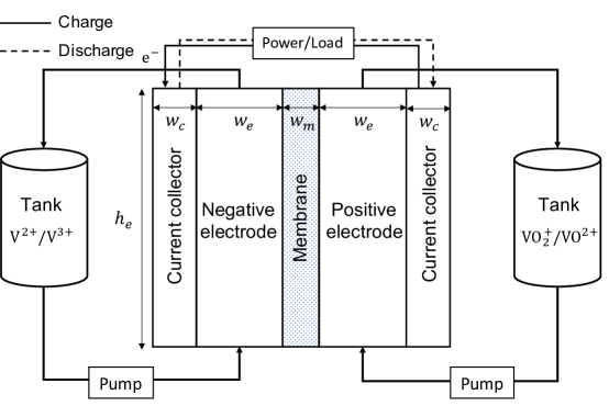
Figure 1: Schematic diagram of a single-cell vanadium redox flow battery (VRFB), which is composed of current collectors, positive and negative electrodes, electrolyte tanks (reservoirs), and an ion exchange membrane.

In this study, the 0D VRFB model [10] is adopted to describe the reaction kinetics in the electrolytes, electrodes, and membrane of a single-cell VRFB (see Fig. 1). The 0D model is derived based on the mass and energy conservation laws while disregarding the spatial variability of battery properties and electrochemical processes. The latter requires the electrolytes to be sufficiently dilute and be uniformly distributed in the porous electrodes. In addition, two assumptions are made in deriving the 0D governing equations: (1) the electrolytes are circulated at a constant flow rate between the respective electrodes and reservoirs; and (2) the crossover of vanadium ions through the membrane and any other side reactions are not considered in the model.

The main chemical reactions in the VRFB can be summarized as

$$-\text{ve electrode}:\text{V(III)}+\ce{e-}\ce{<=>}\text{V(II)}$$ (1a)

$$+\text{ve electrode}:\ce{VO^{2}+}+\ce{H2O}\ce{<=>}\ce{VO2+}+2\ce{H+}+\ce{e-}$$ (1b)

Let $c_{i},i\in\mathcal{S}=\{\text{V(II)},\text{V(III)},\text{V(IV)},\text{V(V)},\text{H}^{+},\text{H}_{2}\text{O}\}$ denote the concentration of active species $i$ in liquid, where V(IV) and V(V) refer to VO^2+ and VO2+, respectively.

The 0D equations governing the evolution of the concentrations of species $c_{i}$ and their analytical solutions are summarized in A. These equations allow the analytical solutions that express the concentration of each species $c_{i}$ as a function of the state of charge (SOC; defined in (23) as a function of time $t$):

$$\{c_{i}(t)\}_{i\in\mathcal{S}}=\{c_{i}(\text{SOC})\}_{i\in\mathcal{S}}=\left\{\begin{array}[]{ll}&c_{\text{V(II)}}=c_{V}^{0}\times\text{SOC}\\ &c_{\text{V(III)}}=c_{V}^{0}\times(1-\text{SOC})\\ &c_{\text{V(IV)}}=c_{V}^{0}\times(1-\text{SOC})\\ &c_{\text{V(V)}}=c_{V}^{0}\times\text{SOC}\\ &c_{\text{H}^{+}_{n}}=c_{\text{H}^{+}_{n}}^{0}+c_{V}^{0}\times\text{SOC}\\ &c_{\text{H}^{+}_{p}}=c_{\text{H}^{+}_{p}}^{0}+c_{V}^{0}\times\text{SOC}\\ &c_{\text{H}_{2}\text{O}_{p}}=c_{\text{H}_{2}\text{O}_{p}}^{0}-(1+n_{d})c_{V}^{0}\times\text{SOC}\end{array}\right.$$ (2)

where $c_{V}^{0}$, $c_{\text{H}^{+}_{n}}^{0}$ ($c_{\text{H}^{+}_{p}}^{0}$), and $c_{\text{H}_{2}\text{O}_{p}}^{0}$ are the initial concentrations of the vanadium, proton, and water species, respectively. The subscripts "$n$" and "$p$" are used to denote the quantities associated with the negative and positive electrodes, e.g., $c_{\text{H}^{+}_{p}}$ represents the concentration of protons $[\ce{H+}]$ in the positive electrode. The initial concentration $c_{V}^{0}$ is equal to the total vanadium concentration in the half cell.

2.2 Cell voltage equations

The cell voltage in VRFB can be computed as  [10, 11, 12, 13]:

$$E^{cell}=E^{OCV}+\eta^{act}+\eta^{ohm}$$ (3)

where $E^{OCV}$ is the reversible open circuit voltage (OCV), $\eta^{act}$ is the activation overpotential, and $\eta^{ohm}$ is the ohmic loss. Eq. (3) ignores the effect of the concentration loss, which is negligible for relatively low current densities.

In Eq. (3), $E^{OCV}$ can be approximated using a full version of Nernst’s equation with the Donnan potential arising across the membrane due to the differences in proton activities between both half-cells [40]:

$$E^{OCV}=E_{p}^{0}-E_{n}^{0}+\frac{RT}{F}\ln\left(\frac{c_{\text{V(II)}}c_{\text{V(V)}}c_{\text{H}^{+}_{p}}c^{2}_{\text{H}^{+}_{p}}}{c_{\text{V(III)}}c_{\text{V(IV)}}c_{\text{H}^{+}_{n}}c_{\text{H}_{2}\text{O}_{p}}}\right)$$ (4)

where $R$, $T$, and $F$ are the ideal gas constant, temperature, and Faraday constant, respectively, and $E_{n}^{0}$ and $E_{p}^{0}$ are the standard potentials. Because protons in the positive electrolyte are undergoing a redox reaction to form water, the proton-water redox couple is also considered in Eq. (4).

The activation overpotential in Eq. (3) is described by the Butler-Volmer equations [41] as:

$$\eta^{act}=\eta_{p}-\eta_{n}$$ (5)

$$\eta_{n}=-\frac{RT}{\alpha F}\operatorname{arcsinh}\left(\frac{j}{2Fk_{n}\sqrt{c_{\text{V(II)}}c_{\text{V(III)}}}}\right)$$ (6)

$$\eta_{p}=\frac{RT}{\alpha F}\operatorname{arcsinh}\left(\frac{j}{2Fk_{p}\sqrt{c_{\text{V(IV)}}c_{\text{V(V)}}}}\right)$$ (7)

where the transfer coefficient $\alpha$ for both electrodes is taken to be 0.5, and $k_{n}$ and $k_{p}$ are the rate constants associated with the reactions at the positive and negative electrodes, respectively. The (local) current density $j$ is calculated by $j=I/A_{s}$ with $A_{s}=SV_{e}$, where $V_{e}$ is the volume of the electrode and $S$ is the specific surface area. An empirical expression for the reaction rate coefficients is given in  [10].

$$k_{n}=k_{n,ref}\exp\left(-\frac{FE_{n}^{0}(T_{ref})}{R}\left[\frac{1}{T_{ref}}-\frac{1}{T}\right]\right)$$ (8)

and

$$k_{p}=k_{p,ref}\exp\left(\frac{FE_{p}^{0}(T_{ref})}{R}\left[\frac{1}{T_{ref}}-\frac{1}{T}\right]\right),$$ (9)

where $k_{n,ref}$ and $k_{p,ref}$ are the reference rate constants for the reactions in Eqs. (1a) and (1b) at $T_{ref}=293$ K, respectively.

The ohmic losses associated with the current collector (c), membrane (m), and electrolyte (e) can be expressed as  [10, 11]:

$$\eta^{ohm}=\left(\frac{2w_{c}}{\sigma_{c}}+\frac{w_{m}}{\sigma_{m}}+\frac{2w_{e}}{\sigma_{e}^{eff}}\right)j_{app},$$ (10)

where $j_{app}$ is the nominal current density defined by $j_{app}=I/A_{e}$, and $w_{c}$, $w_{m}$, and $w_{e}$ are the widths of the collectors, membrane, and electrodes, respectively (as illustrated in Fig. 1), and $\sigma_{c}$ is the conductivity of the collector (usually provided by the manufacturers). The Bruggeman correction [42] is used in the effective conductivity of the porous electrode, given by $\sigma_{e}^{eff}=\epsilon^{3/2}\sigma_{e}$. Assuming a fully saturated Nafion membrane [43] with $\lambda=22$, the conductivity of membrane $\sigma_{m}$ can be expressed as [44]:

$$\sigma_{m}=(0.5139\lambda-0.326)\exp\left(1268\left[\frac{1}{303}-\frac{1}{T}\right]\right).$$ (11)

While most of the parameters in the 0D model are independent or weakly dependent on the operating conditions, some parameters, including $\sigma_{e}$, $S$, $k_{n}$, and $k_{p}$, were found to have a strong dependence on the operating conditions [16, 10, 15, 12]. In this work, we use the proposed PCDNN method to model these parameters as functions of operating conditions.

3 Methods & experiments

3.1 Physics-constrained deep neural networks (PCDNNs)

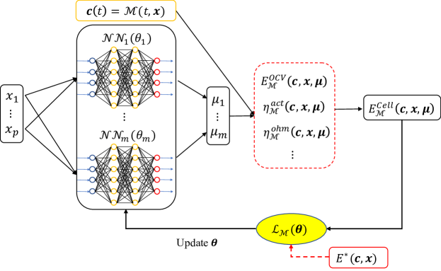
Figure 2: Schematic of the proposed PCDNN approach, where $m$ neural networks are used to relate the operating conditions $\{x_{i}\}_{i=1}^{p}$ and the $m$ identifiable parameters $\{\mu_{i}\}_{i=1}^{m}$ associated with the physics-based electrochemical model. Here, $\mathcal{M}$ denotes a predefined physical model used to compute the concentrations of species $\{c_{i}\}_{i\in\mathcal{S}}$, open circuit voltage $E_{\mathcal{M}}^{\text{OCV}}$, activation overpotential $\eta_{\mathcal{M}}^{\text{act}}$, and ohmic losses $\eta_{\mathcal{M}}^{\text{ohm}}$. Note that the 0D model described in Section 2 is adopted in this study.

The general framework of the PCDNN approach is illustrated in Fig. 2, where the model parameters to be estimated are denoted as $\boldsymbol{\mu}=\{\mu_{i}\}_{i=1}^{m}$, and $\boldsymbol{x}=\{x_{i}\}_{i=1}^{p}$ is the $p$-dimensional vector of the experimental operating conditions for VRFB. Here, we approximate functional relationships between $\mu_{i}$ and the operating conditions $\boldsymbol{x}$ with fully connected feed-forward DNNs:

$$\mu_{i}(\boldsymbol{x})\approx\hat{\mu}_{i}(\boldsymbol{x};\theta_{i})=\mathcal{NN}_{i}(\boldsymbol{x};\theta_{i}),\quad\text{for}\;i=1,...,m$$ (12)

where $\mathcal{NN}_{i}$ is a DNN approximation of $\mu_{i}$, and $\theta_{i}$ are the parameters (weights and biases) of $\mathcal{NN}_{i}$. We denote $\boldsymbol{\theta}=\{\theta_{1},...,\theta_{m}\}$ as the collection of all $\theta_{i}$. A brief review of the fully-connected feed-forward DNN architecture is given in B.

Substituting the DNNs $\hat{\boldsymbol{\mu}}(\boldsymbol{\theta})=\{\hat{\mu}_{i}(\theta_{i})\}_{i=1}^{m}$ in Eq (3) gives the equation for voltage as a function of $\boldsymbol{\theta}$, i.e.,

$$E^{cell}_{\mathcal{M}}(\boldsymbol{c},\boldsymbol{x},\hat{\boldsymbol{\mu}}(\boldsymbol{\theta}))=E^{OCV}_{\mathcal{M}}(\boldsymbol{c},\boldsymbol{x},\hat{\boldsymbol{\mu}}(\boldsymbol{\theta}))+\eta^{act}_{\mathcal{M}}(\boldsymbol{c},\boldsymbol{x},\hat{\boldsymbol{\mu}}(\boldsymbol{\theta}))+\eta^{ohm}_{\mathcal{M}}(\boldsymbol{c},\boldsymbol{x},\hat{\boldsymbol{\mu}}(\boldsymbol{\theta}))$$ (13)

where the subscript $\mathcal{M}$ is used to denote a quantity related to the defined physical models.

Considering the concentration–SOC relationship in Eq. (2) and the SOC–time relationship in Eq. (23), the species concentrations can be written as $c_{i}(t,\boldsymbol{x})=c_{i}(\text{SOC}(t,\boldsymbol{x}),\boldsymbol{x})$, and thus, the cell voltage becomes $E^{cell}_{\mathcal{M}}(t,\boldsymbol{x};\boldsymbol{\theta})$.

The DNN parameters $\boldsymbol{\theta}$ in PCDNN are estimated by minimizing the loss function $\mathcal{L}_{\mathcal{M}}$:

$$\boldsymbol{\theta}=\text{arg}\min_{\boldsymbol{\theta}^{*}}\mathcal{L}_{\mathcal{M}}(\boldsymbol{\theta}^{*})=\frac{1}{N^{x}N^{t}_{q}}\sum_{q=1}^{N^{x}}\sum_{l=1}^{N^{t}_{q}}[E^{cell}_{\mathcal{M}}(t_{l},\boldsymbol{x}_{q};\boldsymbol{\theta}^{*})-E^{*}(t_{l},\boldsymbol{x}_{q})]^{2}$$ (14)

where $E^{*}$ are the experimental measurements of the cell voltage, $N^{x}$ is the number of experiments with different operating conditions, $N^{t}_{q}$ is the number of measurements within a charge-discharge process in each experiment, and $t_{l}$ ($l=1,...,N_{q}^{t}$) are times where the measurements are collected. If we define a new array $\boldsymbol{z}=(t,\boldsymbol{x})$ to encode both the input time variable $t$ and the operating conditions $\boldsymbol{x}$, the loss function can be simplified as:

$$\mathcal{L}_{\mathcal{M}}(\boldsymbol{\theta})=\frac{1}{N}\sum_{n=1}^{N}[E^{cell}_{\mathcal{M}}(\boldsymbol{z}_{n},\boldsymbol{\theta})-E^{*}(\boldsymbol{z}_{n})]^{2},$$ (15)

where $N$ is the total number of the measurements. We use gradient descent minimization algorithms, including L-BFGS-B [45] and Adam [46] methods, to minimize $\mathcal{L}_{\mathcal{M}}$. To alleviate potential overfitting, we adopt the $L_{2}$ regularization on $\boldsymbol{\theta}$ [35] with a penalty parameter $10^{-8}$ in the loss function. Once $\boldsymbol{\theta}$ is found, the model parameters can be computed using the DNN $\hat{\boldsymbol{\mu}}(\boldsymbol{x};\boldsymbol{\theta})$ for any given operating conditions $\boldsymbol{x}$.

In this work, we attempt to learn four model parameters including the specific area $S$, the reaction rate constants $k_{n}$ and $k_{p}$, and $\sigma_{e}$, such that $\boldsymbol{\mu}=(S,k_{n},k_{p},\sigma_{e})$. Furthermore, we assume that the parameters $\boldsymbol{\mu}$ depend on the following operating conditions: the average electrolyte flow velocity $\tilde{u}$ ($\tilde{u}=\omega/A_{in}$, see A); the applied current $I$; and the initial vanadium concentration $c^{0}_{V}$. Therefore, the vector of operating conditions is $\boldsymbol{x}=\{\tilde{u},I,c^{0}_{V}\}$. The choice of parameters and operating conditions is based on the reported dependence of $S$, $k_{n}$, $k_{p}$, and $\sigma_{e}$ on $\tilde{u}$, $I$, and $c^{0}_{V}$, as discussed in Section 2.2. Furthermore, it is shown in [28] that the voltage prediction has a relatively high sensitivity with respect to the selected parameters.

3.2 Parameter normalization

Because the parameters $\boldsymbol{\mu}$ are positive-valued functions, we introduce the following expression for $\hat{\mu}_{i}$ in (12) to enforce its positivity in the PCDNN model:

$$\hat{\mu}_{i}(\boldsymbol{x})=\mu_{i}^{0}\exp\left({y_{i}(\boldsymbol{x})}\right),\quad\text{for}\;i=1,...,4,$$ (16)

where the variables $y_{i}(\boldsymbol{x})$ are approximated with DNNs as

$$y_{i}(\boldsymbol{x})=\hat{y}_{i}(\boldsymbol{x},\theta_{i}),\quad\text{for}\;i=1,...,4.$$ (17)

and $(\mu_{1}^{0},\mu_{2}^{0},\mu_{3}^{0},\mu_{4}^{0})=(S^{0},k_{n}^{0},k_{p}^{0},\sigma_{e}^{0})$ are the predefined baseline parameters that we define as the parameters’ values taken from the literature (or, this could be the averages of the parameter values that are reported in the literature).

3.3 Experiment

Table 1: Summary of operating conditions and VRFB parameters for the 12 experiment cases (ID 1-12) for a single cell structure conducted at Pacific Northwest National Laboratory (PNNL). The membrane width is $w_{m}=1.27\times 10^{-2}$ for Nafion 115 and $w_{m}=5.08\times 10^{-3}$ cm for Nafion 212, respectively. The operating temperature is assumed to be $T=298K$.

Exp. Case	$c^{0}_{V}$	$c_{\text{H}^{+}_{p}}^{0}$	$c_{\text{H}^{+}_{n}}^{0}$	$c_{\text{H}_{2}\text{O},p}$	$c_{\text{H}_{2}\text{O},n}$	$\omega$	I	$V_{r}$	Membrane
ID	[mol $\text{m}^{-3}$]	[mol $\text{m}^{-3}$]	[mol $\text{m}^{-3}$]	[mol $\text{m}^{-3}$]	[mol $\text{m}^{-3}$]	[ml $\text{min}^{-1}$]	[A ]	[$\text{m}^{3}$]
1	$1.5\times 10^{3}$	$3.85\times 10^{3}$	$3.03\times 10^{3}$	$4.46\times 10^{4}$	$4.61\times 10^{4}$	30	0.5	$2\times 10^{-5}$	Nafion 115
2	$1.5\times 10^{3}$	$3.85\times 10^{3}$	$3.03\times 10^{3}$	$4.46\times 10^{4}$	$4.61\times 10^{4}$	20	0.75	$8\times 10^{-5}$	Nafion 115
3	$2\times 10^{3}$	$5\times 10^{3}$	$3\times 10^{3}$	$4.75\times 10^{4}$	$4.95\times 10^{4}$	20	0.5	$5\times 10^{-5}$	Nafion 115
4	$2\times 10^{3}$	$5\times 10^{3}$	$3\times 10^{3}$	$4.75\times 10^{4}$	$4.95\times 10^{4}$	20	0.69	$4.5\times 10^{-5}$	Nafion 115
5	$2\times 10^{3}$	$5\times 10^{3}$	$3\times 10^{3}$	$4.75\times 10^{4}$	$4.95\times 10^{4}$	20	0.75	$4.5\times 10^{-5}$	Nafion 115
6	$2\times 10^{3}$	$5\times 10^{3}$	$3\times 10^{3}$	$4.75\times 10^{4}$	$4.95\times 10^{4}$	20	1.5	$4.5\times 10^{-5}$	Nafion 115
7	$2\times 10^{3}$	$5\times 10^{3}$	$3\times 10^{3}$	$4.75\times 10^{4}$	$4.95\times 10^{4}$	20	0.5	$5\times 10^{-5}$	Nafion 212
8	$2\times 10^{3}$	$5\times 10^{3}$	$3\times 10^{3}$	$4.75\times 10^{4}$	$4.95\times 10^{4}$	20	0.4	$3\times 10^{-5}$	Nafion 212
9	$2\times 10^{3}$	$5\times 10^{3}$	$3\times 10^{3}$	$4.75\times 10^{4}$	$4.95\times 10^{4}$	20	0.4	$2.5\times 10^{-5}$	Nafion 212
10	$2\times 10^{3}$	$5\times 10^{3}$	$3\times 10^{3}$	$4.75\times 10^{4}$	$4.95\times 10^{4}$	20	0.5	$4\times 10^{-5}$	Nafion 212
11	$2\times 10^{3}$	$5\times 10^{3}$	$3\times 10^{3}$	$4.75\times 10^{4}$	$4.95\times 10^{4}$	20	1.0	$2\times 10^{-5}$	Nafion 212
12	$1.5\times 10^{3}$	$3.85\times 10^{3}$	$3.03\times 10^{3}$	$4.46\times 10^{4}$	$4.61\times 10^{4}$	20	0.4	$3\times 10^{-5}$	Nafion 212

In this study, we focus on analyzing 12 VRFB experiments [26] that use a cell like the one depicted in Fig. 1. The experimental settings and conditions of each case are summarized in Table 1. In these experiments, the electrolyte was made of 1.5M $\text{VOSO}_{4}$ (Aldrich, 99%) dissolved in 3.5M $\text{H}_{2}\text{S}\text{O}_{4}$ solution (Aldrich, 96-98%). All experiments were run at room temperature. The VRFB single cell was composed of two current collectors with the thickness of $w_{c}=1.5$ cm, two carbon felt electrodes (each $5\times 4\times 0.4$ cm), two reservoir tanks, and a membrane. The electrode area is $A_{e}=20$ $\text{cm}^{2}$. The Nafion 115 and 212 membranes with thickneses $w_{m}=1.27\times 10^{-2}$ and $5.08\times 10^{-3}$ cm, respectively, were used.

The cell voltage $E$ as a function of time (and converted to SOC using the relation in (23)) was measured during each charge-discharge cycle. The experimental results show that the first two charge-discharge cycles may exhibit poor Coulombic efficiency. Thus, we train the PCDNN model using measurements collected during the third cycle. The SOC-V data for the third cycle are plotted in Fig. 3. In Section 4.2, we use the experimental data to demonstrate the accuracy of PCDNN approach.

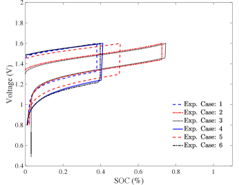
(a)

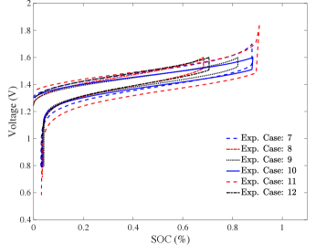
(b)

Figure 3: The measured charge-discharge curves (third cycle) for the 12 PNNL experiments given in Table 1.

3.4 Data availability

The data that support the findings of this study are available from the corresponding author upon request.

4 Results

As mentioned above, the values of the parameters $\sigma_{e}$, $S$, $k_{n}$, and $k_{p}$ vary significantly in different studies. In addition to dependence on the operating conditions, a reason for this variation is the ill-posed nature of multiple-parameter estimation problems that often do not have a unique solution without proper regularization. In Section 4.1, we use synthetic data simulated with the 0D model to demonstrate that the PCDNN method provides necessary regularization to obtain accurate estimates of parameters when the parameter dependence on the operating conditions is not pronounced.

In Section 4.2, we use the PCDNN method to learn parameters as functions of the operating conditions using the experimental data described in Section 3.3.

4.1 Parameter estimation for simulation data

Table 2: Model parameters for the simulation data of the VRFB cell [12].

Symbol	Description	Unit	Values
$E_{p}^{0}$	Standard equilibrium potential (Positive)	V	$1.004$
$E_{n}^{0}$	Standard equilibrium potential (Negative)	V	$-0.26$
$n_{d}$	Drag coefficient	-	$2.5$
$k_{p}$	Standard rate constant at $303$ K (Positive)	m $\text{s}^{-1}$	$1.114\times 10^{-4}$
$k_{n}$	Standard rate constant at $303$ K (Negative)	m $\text{s}^{-1}$	$1.798\times 10^{-5}$
$S$	Specific surface area	$\text{m}^{-1}$	$420$
$\epsilon$	Porosity	-	$0.67$
$\sigma_{e}$	Electrode conductivity	S $\text{m}^{-1}$	$1000$
$\sigma_{c}$	Current collector conductivity	S $\text{m}^{-1}$	$9.1\times 10^{4}$
$T_{ref}$	Reference temperature	$K$	$293$
$A_{e}$	Electrode area	$\text{m}^{2}$	$0.0025$
$w_{e}$	Electrode width	m	$0.003$
$w_{m}$	Membrane width	m	$1.25\times 10^{-4}$
$w_{c}$	Current collector width	m	$0.015$
$V_{r}$	Reservoir volume	$\text{m}^{3}$	$1\times 10^{-4}$

Table 3: Operating conditions for the simulation data of the VRFB cell [12].

Symbol	Description	Unit	Reference values	Test range [Min, Max]
$\omega$	Volumetric flow rate	$\text{m}^{3}$ $\text{s}^{-1}$	$4.17\times 10^{-7}$	-
$j$	Current density	A $\text{m}^{-2}$	$300$	[200,600]
$c_{V}^{0}$	Initial vanadium concentration	mol $\text{m}^{-3}$	$500$	-
$c_{\text{H}^{+}_{n}}^{0}$	Initial $\text{H}^{+}$ concentration (negative)	mol $\text{m}^{-3}$	$6000$	-
$c_{\text{H}^{+}_{p}}^{0}$	Initial $\text{H}^{+}$ concentration (positive)	mol $\text{m}^{-3}$	$6000$	-
$c_{\text{H}_{2}\text{O}}$	Initial $\text{H}_{2}\text{O}$ concentration	mol $\text{m}^{-3}$	$4.6\times 10^{4}$	-
$T$	Temperature	$K$	$303$	-

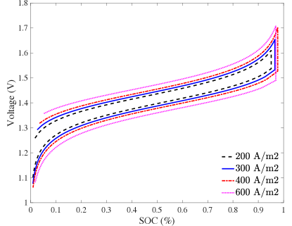
Figure 4: The SOC-V curves for different applied current densities ($j=200$, $300$, $400$, $600$ $\text{A}/\text{m}^{2}$) simulated by the ground truth 0D VRFB model. The numbers of data points for these four cases are 494, 494, 492, and 470, respectively.

To examine the accuracy of the proposed method for parameter estimation, we first test PCDNN using a simulation dataset consisting of four charge-discharge curves (see Fig. 4) that are generated by the 0D VRFB model with the current densities $j=200$, 300, 400, and $600\text{A}/\text{m}^{2}$. The 0D model parameters are taken from [12] and listed in Table 2, and the operating conditions are given in Table 3. The parameter values $\boldsymbol{\mu}=(S,k_{n},k_{p},\sigma_{e})$ given in Table 2 are treated as ground truth and are used to simulate synthetic data (i.e., the ground truth values of $E^{cell}$). The simulation data are used to perform parameter identification, and the estimated parameters are then compared against the ground truth parameters to validate the PCDNN method.

We use the SOC-V curves corresponding to $j=200$ and $400\text{A}/\text{m}^{2}$ as a training set and the rest of the dataset to test the model. To demonstrate that the PCDNN is not very sensitive to the choice of the baseline parameters $\boldsymbol{\mu}_{0}$ with respect to the ground truth, we select the baseline parameter values $S=1\times 10^{3}$ m^-1, $k_{n}=5\times 10^{-5}$ $\text{m}\text{s}^{-1}$, $k_{p}=1\times 10^{-4}$ $\text{m}\text{s}^{-1}$, and $\sigma_{e}=0.5\times 10^{3}$ $\text{S}\text{m}^{-1}$ that are different but within the same order of magnitude of the ground truth parameter values.

Table 4: The RMSE and estimated parameters obtained by PCDNN using different DNN sizes. The results given by the baseline and the least square estimation (LSE) are also provided as comparison. RMSE is evaluated on the test dataset. The ground truth parameters are: $S=4.2\times 10^{2}$, $k_{n}=1.798\times 10^{-5}$, $k_{p}=1.114\times 10^{-4}$, and $\sigma_{e}=1.000\times 10^{3}$.

DNN size	RMSE	$S$ [$\text{m}^{-1}$]	$k_{n}$ [m $\text{s}^{-1}$]	$k_{p}$ [m $\text{s}^{-1}$]	$\sigma_{e}$ [S $\text{m}^{-1}$]
$2\times 20$	$1.555\times 10^{-7}$	$4.1301\times 10^{2}$	$1.8285\times 10^{-5}$	$1.1334\times 10^{-4}$	$1.0000\times 10^{3}$
$2\times 30$	$0.626\times 10^{-7}$	$4.1323\times 10^{2}$	$1.8275\times 10^{-5}$	$1.1328\times 10^{-4}$	$1.0000\times 10^{3}$
$2\times 40$	$2.256\times 10^{-7}$	$4.1370\times 10^{2}$	$1.8254\times 10^{-5}$	$1.1315\times 10^{-4}$	$1.0001\times 10^{3}$
$3\times 20$	$0.784\times 10^{-7}$	$4.1570\times 10^{2}$	$1.8167\times 10^{-5}$	$1.1260\times 10^{-4}$	$1.0000\times 10^{3}$
$3\times 30$	$1.720\times 10^{-7}$	$4.1663\times 10^{2}$	$1.8126\times 10^{-5}$	$1.1236\times 10^{-4}$	$1.0001\times 10^{3}$
$3\times 40$	$2.203\times 10^{-7}$	$4.1188\times 10^{2}$	$1.8335\times 10^{-5}$	$1.1364\times 10^{-4}$	$0.9998\times 10^{3}$
Baseline	$2.477\times 10^{-2}$	$1.000\times 10^{3}$	$5.000\times 10^{-5}$	$1.000\times 10^{-4}$	$0.500\times 10^{3}$
LSE	$1.244\times 10^{-7}$	$5.2201\times 10^{2}$	$1.4467\times 10^{-5}$	$0.89671\times 10^{-4}$	$1.0001\times 10^{3}$

The structure of DNNs for $\hat{\mu}_{i}$ in Eq. (16) is denoted as $n_{l}\times m_{l}$, where $n_{l}$ is the number of hidden layers and $m_{l}$ is the number of neurons per layer. More information about setting the DNN can be found in B. Because the size of the training data is relatively small ($N=986$), the L-BFGS-B optimizer is adopted to train the PCDNN model. The accuracy of the PCDNN prediction is given in terms of the root-mean-square error (RMSE) of the voltage prediction with respect to the reference test data.

Table 4 summarizes the RMSE and the four estimated parameters as functions of the DNN size. It shows that for all considered DNN sizes, the PCDNN method yields accurate cell voltage predictions, as evidenced by the RMSE on the order of $10^{-7}$. On the other hand, the 0D model prediction with the baseline parameters $\boldsymbol{\mu}^{0}$ yields RMSE = $2.477\times 10^{-2}$. The PCDNN predictions are practically independent of the DNN sizes, with the $3\times 30$ DNNs giving the best estimated parameters. In the rest of the paper, we fix the DNN size to be $3\times 30$ unless stated otherwise.

In addition, the numerical results show that the parameters estimated by PCDNN remain unchanged for different current density. This independence is expected because the synthetic data came from experiments that use operation-condition-independent parameter values.

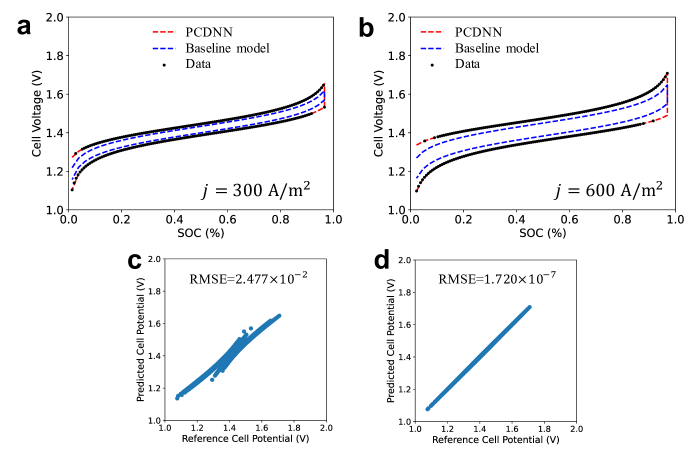
Figure 5: The comparison of cell voltage predictions obtained by the trained PCDNN model and the baseline 0D model with $\boldsymbol{\mu}^{0}$. The predicted SOC-V curves for the test cases $j=300$ $\text{A}/\text{m}^{2}$ and $j=600$ $\text{A}/\text{m}^{2}$ are depicted in (a) and (b), respectively. (c) "one-one" plot to compare the voltage prediction by the baseline 0D model against the test data set. (d) "one-one" plot to compare the voltage prediction by the trained PCDNN model against the test data set. The DNN structure $3\times 30$ is used for the PCDNN model, and the estimated parameters are shown in Table 4.

Because we know that the ground truth parameters are the same for all cases in the simulation data, we can consider the standard least square estimation (LSE) approach for comparison [47, 30]. In the LSE approach, the parameters are found by solving the least square minimization problem,

$$\min_{\{\mu_{i}\}_{i=1}^{m}}\frac{1}{N}\sum_{n=1}^{N}[E^{cell}_{\mathcal{M}}(\{\mu_{i}\}_{i=1}^{m};\boldsymbol{z}_{n})-E^{*}(\boldsymbol{z}_{n})]^{2}.$$ (18)

Table 4 shows that the LSE approach identifies a set of parameters that results in an accurate voltage prediction with RMSE = $2.203\times 10^{-7}$, which is of the same order as RMSE in the PCDNN method. However, the parameters estimated by PCDNN are much closer to the ground truth parameters (see Table 4) than those from the LSE method, suggesting an improvement in PCDNNs over the standard LSE approach for this multiple parameter estimation problem.

Cell voltages predicted with the PCDNN model (with the DNN size $3\times 30$) for $j=300$ and $600$ $\text{A}/\text{m}^{2}$ are shown in Fig. 5a and b, respectively. Fig. 5c and d present the "one-one" plots of the baseline 0D and PCDNN models predictions of $E^{cell}$ against the test dataset values of $E^{cell}$, respectively. Fig. 5 shows that the PCDNN approach substantially improves the voltage prediction for different current density cases relative to the baseline 0D model.

Next, we study the sensitivity of the PCDNN and LSE methods with respect to the number of unknown parameters. We do this by considering a case where only $S$, $k_{n}$, and $\sigma_{e}$ as unknown, while $k_{p}$ is set to its ground truth value $1.114\times 10^{-4}$. The PCDNN approach estimates the three parameters as $S=4.1725\times 10^{2}$, $k_{n}=1.8097\times 10^{-5}$, and $\sigma_{e}=1.0002\times 10^{3}$, which are close to the values that these parameters estimated in Table 4 where the number of unknown parameters was set to 4. On the other hand, the LSE approach yields the vales $S=4.2179\times 10^{2}$, $k_{n}=1.7904\times 10^{-5}$, and $\sigma_{e}=0.9998\times 10^{3}$, which are significantly different from the values of these parameters in Table 4 and closer to the ground truth values.

The inverse problem with three unknown parameters is significantly simpler than the one with four unknown parameters because of a nonlinear dependence between $k_{p}$ and $k_{n}$ in (5) for the activation overpotential. These results show that the proposed PCDNN approach outperforms the standard LSE method by being less sensitive to the number of unknown parameters and a nonlinear dependence between the unknown parameters.

It must be pointed out that in this case, the values of model parameters that need to be learned by the DNNs are constant and fixed to their ground truth values. We also note that with both PCDNN and LSE, the parameter $\sigma_{e}$ is estimated more accurately than the other parameters. This is because the dependence of $E^{cell}$ on $\sigma_{e}$ is simpler than on the rest of the parameters.

4.2 Learning parameters as functions of operating conditions from experimental data

Here, we consider the 12 experiments described in Section 3.3, with the operating conditions and the known (measured) VRFB parameters summarized in Table 1. In all considered experiments, $A_{e}=20$ $\text{cm}^{2}$, $w_{e}=0.4$ cm, $w_{c}=1.5$ cm, and temperature are assumed to be constant $T=298$ $K$. All other parameters that are required for the 0D model of these experiments are given in Table 2.

The baseline values $\boldsymbol{\mu}^{0}$ of the unknown 0D model parameters are taken from [25] and listed in Table 5. This table also lists a physically admissible range for each unknown parameter $\mu_{i}$, where the upper and lower bounds are estimated according to [28] based on the previous studies reported in [8, 10, 17, 12, 13, 25].

Given the large number of operating conditions (Table 1), $E^{cell}$ varies significantly in the experiments, as shown in Fig. 3. It is neither practical nor very useful to perform parameter fitting for each experiment because of the ill-posed nature of the parameter estimation problem. Thus, the proposed PCDNN method is used to learn the model parameters based on the ensemble of experimental data corresponding to the various operating conditions.

Table 5: The baseline values and feasible ranges of the model parameters to be estimated from experiments.

Symbol	Description	Unit	Baseline values [25]	Test range [Min, Max] [28]
$S$	Active surface area	$\text{m}^{-1}$	$3.48\times 10^{4}$	$[1.62\times 10^{3},1.62\times 10^{5}]$
$k_{n}$	Standard rate constant at $T$ (Negative)	m $\text{s}^{-1}$	$5.0\times 10^{-8}$	$[1.7\times 10^{-8},6.8\times 10^{-6}]$
$k_{p}$	Standard rate constant at $T$ (Positive)	m $\text{s}^{-1}$	$1.0\times 10^{-7}$	$[1.7\times 10^{-8},6.8\times 10^{-6}]$
$\sigma_{e}$	Electrode conductivity	S $\text{m}^{-1}$	$500$	$[1.0\times 10^{2},1.0\times 10^{4}]$

4.2.1 Learning parameters from the experimental dataset

Here, we randomly select 60% data points from the 12 experimental SOC-V curves (see Fig. 3) for training the PCDNN model. The remaining 40% data are used as the test data to evaluate the prediction performance. After training the PCDNN model, we obtain the parameters $\hat{\mu}_{i}(\boldsymbol{x};\theta_{i})$ as functions of the operating conditions $\boldsymbol{x}=\{\tilde{u},I,c^{0}_{V}\}$. Then, the PCDNN estimated model parameters for each experiment can be computed by evaluating $\hat{\mu}_{i}(\boldsymbol{x};\theta_{i})$ for the operating conditions $\boldsymbol{x}$ in the considered experiment.

Table 6: The estimated parameters and the RMSE obtained by the PCDNN approach for the 12 experiments. The constant parameters estimated by LSE are also provided for comparison.

Exp. ID		RMSE	$S$	$k_{n}$	$k_{p}$	$\sigma_{e}$
			PCDNN estimated parameters
1		$2.875\times 10^{-2}$	$2.95\times 10^{4}$	$7.07\times 10^{-8}$	$1.19\times 10^{-7}$	$1.00\times 10^{2}$
2		$1.716\times 10^{-2}$	$3.62\times 10^{4}$	$1.75\times 10^{-7}$	$1.67\times 10^{-7}$	$1.56\times 10^{2}$
3		$7.620\times 10^{-2}$	$2.61\times 10^{4}$	$1.14\times 10^{-7}$	$1.90\times 10^{-7}$	$2.42\times 10^{2}$
4		$6.331\times 10^{-3}$	$2.65\times 10^{4}$	$1.70\times 10^{-8}$	$2.08\times 10^{-7}$	$3.35\times 10^{2}$
5		$9.822\times 10^{-3}$	$2.67\times 10^{4}$	$1.70\times 10^{-8}$	$2.13\times 10^{-7}$	$3.43\times 10^{2}$
6		$7.141\times 10^{-3}$	$2.86\times 10^{4}$	$1.04\times 10^{-7}$	$2.56\times 10^{-7}$	$1.95\times 10^{2}$
7		$3.243\times 10^{-2}$	$2.61\times 10^{4}$	$1.14\times 10^{-7}$	$1.91\times 10^{-7}$	$2.42\times 10^{2}$
8		$3.602\times 10^{-2}$	$2.58\times 10^{4}$	$1.91\times 10^{-7}$	$1.80\times 10^{-7}$	$1.81\times 10^{2}$
9		$3.472\times 10^{-2}$	$2.58\times 10^{4}$	$1.91\times 10^{-7}$	$1.80\times 10^{-7}$	$1.81\times 10^{2}$
10		$3.137\times 10^{-2}$	$2.61\times 10^{4}$	$1.14\times 10^{-7}$	$1.91\times 10^{-7}$	$2.42\times 10^{2}$
11		$6.403\times 10^{-3}$	$1.51\times 10^{4}$	$1.51\times 10^{-7}$	$2.31\times 10^{-7}$	$3.21\times 10^{2}$
12		$3.836\times 10^{-2}$	$3.56\times 10^{4}$	$1.38\times 10^{-6}$	$1.46\times 10^{-7}$	$1.00\times 10^{2}$
LSE (all cases)			$3.04\times 10^{4}$	$2.90\times 10^{-8}$	$1.38\times 10^{-7}$	$5.68\times 10^{2}$

The estimated parameters of the PCDNN model for the whole dataset (i.e., all 12 experiments) are given in Table 6. It can be seen that, among the four estimated parameters, $S$ has the smallest range of values. This can be explained by the fact that these experiments adopt the same carbon fiber electrodes, and the variations are mainly due to different flow rates that affect the spatial distribution of species in the electrodes.

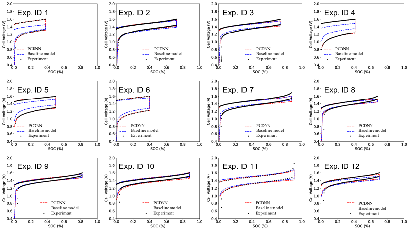
Figure 6: The comparison of SOC-V predictions for all 12 experiments by the PCDNN model (dashed red line) and the VRFB 0D model (dashed blue line) using the baseline parameters in Table 5. The black dots denote the experimental data.

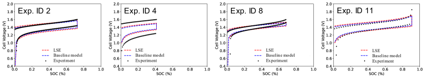
Figure 7: The comparison of SOC-V predictions for exemplary experiments by the VRFB 0D model using the LSE estimated parameters (dashed red line) in Table 6 and the baseline parameters (dashed blue line) in Table 5. The black dots denote the experimental data.

With the various estimated parameters, the RMSE of the PCDNN voltage prediction against the test data is $3.267\times 10^{-2}$, which is about $35\%$ and $40\%$ smaller than those of the standard LSE approach and the baseline VRFB 0D model, respectively. Fig. 6 shows that the PCDNN voltage prediction agrees well with the experimental data for experiments 1-6 (that use the Nafion 115 membrane) for the entire range of SOC values and is significantly better than the baseline 0D model predictions. For experiments 7–12, there are some discrepancies between the PCDNN predictions and experimental data for very small and large SOC values. These discrepancies are due to simplifications in the 0D model and cannot be corrected through the choice of different values for the 0D model parameters. However, these results show that the proposed approach improves the prediction of the 0D model with constant parameters for all considered experiments. Also, it is important to note that using higher-dimensional flow models instead of the 0D model should further improve the predictive ability of the proposed approach.

We also note that the standard LSE approach hardly improves the voltage prediction compared to the baseline 0D model using values from the literature as illustrated in Fig. 7 for experiments 2, 4, 8, and 11.

4.2.2 Leave-one-out testing of the DNN parameter models

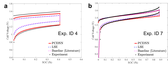
Figure 8: The comparison of SOC-V predictions for experiments (Cases 4 and 7) by using PCDNN and LSE parameter estimation approaches. The VRFB 0D model (dashed blue line) using the baseline parameters in Table 5 is also provided.

Table 7: The comparison of the RMSE and estimated parameters by the PCDNN and LSE approaches for different experiment cases.

	RMSE	$S$	$k_{n}$	$k_{p}$	$\sigma_{e}$
Baseline model∗
Exp. ID 4	$1.271\times 10^{-1}$	$3.48\times 10^{4}$	$5.00\times 10^{-8}$	$1.00\times 10^{-7}$	$5.00\times 10^{2}$
Exp. ID 7	$3.651\times 10^{-2}$
Least-square estimation
Exp. ID 4	$1.152\times 10^{-1}$	$2.91\times 10^{4}$	$5.31\times 10^{-8}$	$5.23\times 10^{-8}$	$1.29\times 10^{3}$
Exp. ID 7	$3.274\times 10^{-2}$
PCDNN
Exp. ID 4	$4.097\times 10^{-2}$	$3.01\times 10^{4}$	$1.70\times 10^{-8}$	$3.33\times 10^{-7}$	$1.00\times 10^{4}$
Exp. ID 7	$3.357\times 10^{-2}$	$2.93\times 10^{4}$	$2.42\times 10^{-8}$	$5.30\times 10^{-7}$	$1.00\times 10^{4}$

^∗ use the baseline parameters in Table 5

In this section, we investigate the effectiveness of the proposed PCDNN approach for modeling new or unseen experiments using the leave-one-out approach. That is, the PCDNN model is used to predict experiments with operating conditions different from those in the training dataset. Figure 8 and Table 7 show a detailed analysis of the leave-one-out tests for experiments 4 and 7. Table 8 gives RMSE in the leave-one-out tests for all 12 experiments.

We select experiments 4 and 7 for the detailed analysis because they are performed under different operation conditions and use different membranes: the Nafion 115 membrane in experiment 4 and Nafion 212 in experiment 7. Figure 8 shows the cell voltage for the test experiments as predicted by the PCDNN approach. Although no measurement data associated with the test experiments (Cases 4 and 7) are included in training the PCDNN model, the PCDNN prediction shows an improved agreement with the experimental data compared to the baseline 0D model. The RMSEs of the PCDNN approach for experiments 4 and 7 are $4.097\times 10^{-2}$ and $3.357\times 10^{-2}$, respectively, which are smaller than the RMSEs $1.271\times 10^{-1}$ and $3.651\times 10^{-2}$ in the baseline 0D model. Also, these results show that the LSE approach is less effective than PCDNN in predicting the voltage responses for the fourth experiment, as shown in Fig. 8a, where its RMSE is $1.152\times 10^{-1}$.

Table 8: RMSE in the voltage estimated with the 0D model with the PCDNN and LSE parameterazation for the 12 experiments in the leave-one-out test. For comparison, RMSE in the estimated voltage with the baseline 0D model is also shown.

Exp. ID	Baseline model∗	Least-square estimation	PCDNN
1	$1.036\times 10^{-1}$	$9.035\times 10^{-2}$	$2.865\times 10^{-2}$
2	$2.641\times 10^{-2}$	$3.508\times 10^{-2}$	$1.682\times 10^{-2}$
3	$8.707\times 10^{-2}$	$8.235\times 10^{-2}$	$7.552\times 10^{-2}$
4	$1.271\times 10^{-1}$	$1.152\times 10^{-1}$	$4.097\times 10^{-2}$
5	$8.957\times 10^{-2}$	$7.836\times 10^{-2}$	$9.115\times 10^{-3}$
6	$5.367\times 10^{-2}$	$4.500\times 10^{-2}$	$6.982\times 10^{-3}$
7	$3.651\times 10^{-2}$	$3.274\times 10^{-2}$	$3.357\times 10^{-2}$
8	$3.906\times 10^{-2}$	$3.835\times 10^{-2}$	$3.751\times 10^{-2}$
9	$3.590\times 10^{-2}$	$3.609\times 10^{-2}$	$3.462\times 10^{-2}$
10	$2.951\times 10^{-2}$	$3.074\times 10^{-2}$	$3.310\times 10^{-2}$
11	$6.988\times 10^{-2}$	$6.758\times 10^{-2}$	$6.336\times 10^{-2}$
12	$4.979\times 10^{-2}$	$4.880\times 10^{-2}$	$3.943\times 10^{-2}$

^∗ use the baseline parameters in Table 5

Table 8 shows the comparison of the RMSE in voltage estimated with the 0D model with the PCDNN and LSE parameteraziations using the leave-one-out approach for all 12 experiments. For comparison, we also show the RMSE in the estimated voltage in the 0D model with the baseline parameters. We can see that even with a relatively small data set (only 11 experiments) the PCDNN model is more accurate than the 0D model with parameters estimated using the LSE method for all but experiments 7 and 10. When compared to the 0D model with baseline parameters, the PCDNN is more accurate for all but the experiment 10. The applications of physics-constrained DNN methods to diffusion and advection-diffusion systems demonstrated that the accuracy of these methods improves with the increasing number of measurements [36, 37]. Therefore, we expect that the accuracy of the PCDNN parameterization versus the LSE paramerization would increase as more data becomes available.

Like many other traditional parameter estimation methods, LSE finds the optimal set of parameters for a single instant of the operating conditions. The approach proposed here allows learning the functional relationships between the model parameters and operating conditions. We note that in general, functions are infinite dimensional, i.e., an infinite number of values are required to represent an unknown function, and using parameter estimation methods like LSE is poorly suited for learning functional relationships.

5 Discussion and Conclusions

We developed a physics-constrained DNN parameter estimation framework for the 0D flow battery model, which enables learning model parameters as functions of operating conditions. In this framework, DNNs are used to approximate the map from the operating conditions to the model parameters, and the 0D VRFB physical model combined with the DNN parameter functions is used to predict the cell voltage. Thus, different from direct data-driven DNN methods that learn a map from the operating conditions to the voltage, the PCDNN model voltage output satisfies the given physical model. The key idea of the proposed approach is to directly learn the parameter functions by training DNNs subject to physics model constraints with the experimental datasets that are collected from many experiments. Therefore, the trained PCDNN model can predict both the model parameters and cell voltage under varying operating condition, including the conditions that are not part of the training dataset. This is different from standard model calibration approaches such as LSE, where modeling a battery under certain operating conditions requires calibrating the model for these same operating conditions. Such model calibration approaches cannot be used to accurately predict battery performance under new conditions when the model parameters have a strong dependence on the operating conditions.

In this work, we demonstrated the effectiveness of the PCDNN approach by using the simulation data generated with reference operating-condition-independent parameters, as discussed in Section 4.1. We demonstrated that the PCDNN approach can estimate such parameters more accurately than the LSE approach. We also demonstrated that the PCDNN method produces equally accurate results for problems with three and four unknown parameters, while the accuracy of the LSE method decreases with an increasing number of unknown parameters. In Section 4.2, we tested the PCDNN approach for an experimental dataset consisting of voltage measurements as functions of time and operating conditions from 12 different experiments. The results show that the PCDNN approach significantly improves the voltage prediction compared to the predictions of the 0D model with parameters reported in the literature [25] and estimated from the LSE approach. The PCDNN method produced more accurate predictions for both the experiments that were used for parameter estimation and the unseen experiments, i.e., those experiments that were not used in the training of the PCDNN model. These results demonstrate the enhanced abilities of parameter estimation and predictive generalization offered by the PCDNN approach, which provides a flexible framework to leverage the information of physical models and experimental data. It also serves as a surrogate model that allows efficient parameter estimation and avoids repeated, time-consuming calibration procedures.

In this work, we used the PCDNN approach to estimate the functional forms of parameters in a simple 0D model that has a limited ability to capture the tails of the charge and discharge curves, noticeable discrepancies in cell voltage predictions were observed at the extreme SOC values in some of the experiments. Considering additional physics in the 0D model, such as the concentration overpotential, can further improve the cell voltage prediction of the “PCDNN-0D” model. We should note that the PCDNN approach can be also used to estimate the functional form of parameters in higher-dimensional physics-based models of flow batteries that would improve these models’ accuracy with respect to standard LSE parametarization; however, this would also require numerically solving the PDEs or approximating the solution of PDEs with a DNN as in the standard PINN method.

Finally, we note that introducing more physics (e.g., concentration overpotential and cross-over) and considering more changing model parameters, such as membrane properties, electronic conductivity, and diffusion coefficients in the electrolyte) in the 0D model could enable the PCDNN method to predict more complex aspects of battery performance, such as degradation.

6 Acknowledgments

The authors thank Litao Yan, Yunxiang Chen, and Jie Bao for helpful discussions. The work was supported by the Energy Storage Materials Initiative (ESMI), which is a Laboratory Directed Research and Development Project at Pacific Northwest National Laboratory. Pacific Northwest National Laboratory is operated by Battelle for the U.S. Department of Energy under Contract DE-AC05-76RL01830.

Appendix A Analytical solution of species concentrations

Following the 0D VRFB model proposed in [10], the species considered in the reaction kinetics are $\mathcal{S}=\{\text{V(II)},\text{V(III)},\text{V(IV)},\text{V(V)},\text{H}^{+},\text{H}_{2}\text{O}\}$. Let $c_{i}^{res}$ and $c_{i}$ be the concentrations of species $i$ ($i\in\mathcal{S}$) in the reservoir and the electrode, respectively. Note that both $c_{i}^{res}$ and $c_{i}$ are space-independent functions because of the assumption of uniform distribution in the 0D model.

With a uniform flow rate at the inlet, the net change per unit time (mol/s) of species $i$ in the electrode due to recirculation is $\epsilon A_{in}u(c_{i}^{res}-c_{i})$, where $\epsilon$ is the porosity of the electrode, $u$ is the electrolyte flow velocity (in m/s), and $A_{in}=b_{e}w_{e}$ is the inlet area of the electrode, in which $b_{e}$ and $w_{e}$ are the breadth and width, respectively. Here, we define $\tilde{u}=\epsilon u=\omega/A_{in}$ as the average velocity in the porous medium, where $\omega$ is the inlet volume flow rate. Therefore, the mass conservation of species $i$ in the reservoirs is:

$$V_{r}\frac{dc_{i}^{res}}{dt}=-A_{in}\tilde{u}(c_{i}^{res}-c_{i})$$ (19)

where $V_{r}$ is the volume of the reservoir.

In the electrodes, we consider both the electrochemical reaction and the recirculation in the mass balance equations for the species ($i=\text{V(II), V(III), V(IV), V(V)}$), expressed as:

$$\epsilon V_{e}\frac{dc_{i}}{dt}=A_{in}\tilde{u}(c_{i}^{res}-c_{i})-\frac{I}{F},\quad i=\text{V(II), V(V)},$$ (20a)

$$\epsilon V_{e}\frac{dc_{i}}{dt}=A_{in}\tilde{u}(c_{i}^{res}-c_{i})+\frac{I}{F},\quad i=\text{V(III), V(IV)},$$ (20b)

where $I$ is the applied current, $V_{e}=b_{e}w_{e}h_{e}$ is the volume of the electrode, and $h_{e}$ is the length of the electrode. Eliminating the recirculation terms in Eqs. (19) and (20) and integrating time using the initial conditions, the solutions for electrode concentrations can be obtained [10]:

$$c_{i}=c_{i}^{0}-\frac{I}{V_{e}F\epsilon\tilde{\epsilon}}\left(\frac{\epsilon\delta+e^{-\tilde{\epsilon}t}}{1+\epsilon\delta}-1-\frac{\epsilon\delta}{\tau}t\right),\quad i=\text{V(II), V(V)},$$ (21a)

$$c_{i}=c_{i}^{0}+\frac{I}{V_{e}F\epsilon\tilde{\epsilon}}\left(\frac{\epsilon\delta+e^{-\tilde{\epsilon}t}}{1+\epsilon\delta}-1-\frac{\epsilon\delta}{\tau}t\right),\quad i=\text{V(III), V(IV)},$$ (21b)

where $c_{i}^{0}$ are the initial concentrations for both $c_{i}^{res}$ and $c_{i}$, $\delta=V_{e}/V_{r}$ is the ratio of the two volumes, $\tau=h_{e}/u$ and $\tilde{\epsilon}=(\epsilon\delta+1)/\tau$. Then, we can define the state of charge (SOC) [16] as

$$\text{SOC}(t)=\frac{c_{\text{V(II)}}(t)}{\bar{c}_{V_{n}}}=1-\frac{c_{\text{V(III)}}(t)}{\bar{c}_{V_{n}}}$$ (22)

where $\bar{c}_{V_{n}}$ is the total vanadium concentration of the negative half-cell. Substituting the analytical solution for $c_{\text{V(II)}}$ from Eq. (21a) into Eq. (22), SOC can be rewritten as

$$\text{SOC}(t)=\text{SOC}^{0}-\frac{I}{\bar{c}_{V_{n}}V_{e}F\epsilon\tilde{\epsilon}}\left(\frac{\epsilon\delta+e^{-\tilde{\epsilon}t}}{1+\epsilon\delta}-1-\frac{\epsilon\delta}{\tau}t\right)$$ (23)

where $\text{SOC}^{0}=c_{\text{V(II)}}^{0}/\bar{c}_{V_{n}}$ is the initial SOC.

A similar procedure is adopted for the concentrations of water and protons, i.e., $c_{\text{H}_{2}\text{O}}$ and $c_{\text{H}^{+}}$. The mass conservation of water is

$$-\text{ve electrode}:\epsilon V_{e}\frac{dc_{\text{H}_{2}\text{O}}}{dt}=A_{in}\tilde{u}(c_{\text{H}_{2}\text{O}}^{res}-c_{\text{H}_{2}\text{O}})+\frac{n_{d}I}{F},$$ (24a)

$$+\text{ve electrode}:\epsilon V_{e}\frac{dc_{\text{H}_{2}\text{O}}}{dt}=A_{in}\tilde{u}(c_{\text{H}_{2}\text{O}}^{res}-c_{\text{H}_{2}\text{O}})-\frac{(1+n_{d})I}{F}.$$ (24b)

Herein, the molar flux of water through the membrane from the positive to negative electrode during charging is approximated by $n_{d}j_{app}/F$, where $n_{d}$ is the drag coefficient, $j_{app}=I/A_{e}$ is the nominal current density, and $A_{e}=h_{e}w_{e}$ is the electrode area. By using the mass balance equation in (19) with $i=\text{H}_{2}\text{O}$ to eliminate the recirculation terms, the solution to Eq. (24) reads

$$-\text{ve electrode}:c_{\text{H}_{2}\text{O}}=c_{\text{H}_{2}\text{O}}^{0}-\frac{In_{d}}{V_{e}F\epsilon\tilde{\epsilon}}\left(\frac{\epsilon\delta+e^{-\tilde{\epsilon}t}}{1+\epsilon\delta}-1-\frac{\epsilon\delta}{\tau}t\right),$$ (25a)

$$+\text{ve electrode}:c_{\text{H}_{2}\text{O}}=c_{\text{H}_{2}\text{O}}^{0}+\frac{I}{V_{e}F\epsilon\tilde{\epsilon}}(1+n_{d})\left(\frac{\epsilon\delta+e^{-\tilde{\epsilon}t}}{1+\epsilon\delta}-1-\frac{\epsilon\delta}{\tau}t\right).$$ (25b)

Using the SOC in Eq. (23), the water concentration in the positive electrode $c_{\text{H}_{2}\text{O}_{p}}$ is expressed as: $c_{\text{H}_{2}\text{O}_{p}}=c_{\text{H}_{2}\text{O}_{p}}^{0}-(1+n_{d})\bar{c}_{V_{n}}\times(\text{SOC}-\text{SOC}^{0})$. The mass balances for the protons are:

$$-\text{ve electrode}:\epsilon V_{e}\frac{dc_{\text{H}^{+}}}{dt}=A_{in}\tilde{u}(c_{\text{H}^{+}}^{res}-c_{\text{H}^{+}})+\frac{I}{F},$$ (26a)

$$+\text{ve electrode}:\epsilon V_{e}\frac{dc_{\text{H}^{+}}}{dt}=A_{in}\tilde{u}(c_{\text{H}^{+}}^{res}-c_{\text{H}^{+}})+\frac{I}{F}.$$ (26b)

For simplicity, in the above equation (26) we assume a rapid transport of protons across the fully saturated membrane such that the protons are evenly distributed in both the positive and negative electrodes, which is different from the original formulation in [10]. Thus, the proton concentrations in both electrodes are:

$$c_{\text{H}^{+}}=c_{\text{H}^{+}}^{0}-\frac{I}{V_{e}F\epsilon\tilde{\epsilon}}\left(\frac{\epsilon\delta+e^{-\tilde{\epsilon}t}}{1+\epsilon\delta}-1-\frac{\epsilon\delta}{\tau}t\right),$$ (27)

or expressed as $c_{\text{H}^{+}}=c_{\text{H}^{+}}^{0}+\bar{c}_{V_{n}}\times(\text{SOC}-\text{SOC}^{0})$.

For the experiments considered in this study, we set the initial concentrations $c_{\text{V(III)}}^{0}=c_{\text{V(IV)}}^{0}=c_{V}^{0}$ and $c_{V}^{0}=\bar{c}_{V_{n}}$. Thus, we have $\text{SOC}^{0}=0$. Then, the SOC estimated by Eqs. (22) and (23) is used to calculate the concentration of each species, as shown in Eq. (2).

Appendix B Deep neural network

In the proposed approach, we use a fully connected feed-forward network architecture known as multilayer perceptrons, where the basic computing units (neurons) are stacked in layers. Generally, the DNN approximation $\hat{\boldsymbol{u}}(\boldsymbol{x};\theta)$ of a function $\boldsymbol{u}(\boldsymbol{x})$ is given as:

$$\boldsymbol{u}(\boldsymbol{x})\approx\hat{\boldsymbol{u}}(\boldsymbol{x};\theta)=\boldsymbol{y}_{n_{l}+1}(\boldsymbol{y}_{n_{l}}(...(\boldsymbol{y}_{2}(\boldsymbol{x}))),$$ (28)

where $\hat{(\cdot)}$ denotes the DNN approximation, and

$$\begin{split}\boldsymbol{y}_{2}(\boldsymbol{x})&=\sigma(\boldsymbol{W}_{1}\boldsymbol{x}+\boldsymbol{b}_{1})\\ \boldsymbol{y}_{3}(\boldsymbol{y}_{2})&=\sigma(\boldsymbol{W}_{2}\boldsymbol{y}_{2}+\boldsymbol{b}_{2})\\ ...\\ \boldsymbol{y}_{n_{l}}(\boldsymbol{y}_{n_{l}-1})&=\sigma(\boldsymbol{W}_{n_{l}-1}\boldsymbol{y}_{n_{l}-1}+\boldsymbol{b}_{n_{l}-1})\\ \boldsymbol{y}_{n_{l}+1}(\boldsymbol{y}_{n_{l}})&=\boldsymbol{W}_{n_{l}}\boldsymbol{y}_{n_{l}}+\boldsymbol{b}_{n_{l}}.\end{split}$$ (29)

The first layer is called the input layer, and the last layer is the output layer, while all the intermediate layers are known as hidden layers. Here, $n_{l}$ denotes the number of hidden layers, $\sigma$ is the predefined activation function, $\boldsymbol{x}\in\mathbb{R}^{d}$ denotes the input ($d$ is the number of spatial dimensions), $\boldsymbol{y}_{n_{l}+1}$ is the output vector, and $\theta$ denotes all the parameters (weights and biases) in the DNN approximation of $\boldsymbol{u}$:

$$\theta=\{\boldsymbol{W}_{1},\boldsymbol{W}_{2},...,\boldsymbol{W}_{n_{l}},\boldsymbol{b}_{1},\boldsymbol{b}_{2},...,\boldsymbol{b}_{n_{l}}\}.$$ (30)

References

- [1] W. Wang, Q. Luo, B. Li, X. Wei, L. Li, Z. Yang, Recent progress in redox flow battery research and development, Advanced Functional Materials 23 (8) (2013) 970–986.
- [2] J. Noack, N. Roznyatovskaya, T. Herr, P. Fischer, The chemistry of redox-flow batteries, Angewandte Chemie International Edition 54 (34) (2015) 9776–9809.
- [3] A. Z. Weber, M. M. Mench, J. P. Meyers, P. N. Ross, J. T. Gostick, Q. Liu, Redox flow batteries: a review, Journal of applied electrochemistry 41 (10) (2011) 1137.
- [4] E. Sum, M. Skyllas-Kazacos, A study of the V (II)/V (III) redox couple for redox flow cell applications, Journal of Power sources 15 (2-3) (1985) 179–190.
- [5] E. Sum, M. Rychcik, M. Skyllas-Kazacos, Investigation of the V (V)/V (IV) system for use in the positive half-cell of a redox battery, J. Power Sources;(Switzerland) 16 (2) (1985).
- [6] M. Skyllas-Kazacos, M. Rychcik, R. G. Robins, A. G. Fane, M. A. Green, New all-vanadium redox flow cell, Journal of the Electrochemical Society 133 (5) (1986) 1057.
- [7] G. Kear, A. A. Shah, F. C. Walsh, Development of the all-vanadium redox flow battery for energy storage: a review of technological, financial and policy aspects, International journal of energy research 36 (11) (2012) 1105–1120.
- [8] A. A. Shah, M. J. Watt-Smith, F. C. Walsh, A dynamic performance model for redox-flow batteries involving soluble species, Electrochimica Acta 53 (27) (2008) 8087–8100. doi:10.1016/j.electacta.2008.05.067.
-
[9]
Q. Zheng, X. Li, Y. Cheng, G. Ning, F. Xing, H. Zhang,
Development and
perspective in vanadium flow battery modeling, Applied Energy 132 (2014)
254–266.
doi:10.1016/j.apenergy.2014.06.077.
URL http://dx.doi.org/10.1016/j.apenergy.2014.06.077 - [10] A. A. Shah, R. Tangirala, R. Singh, R. G. Wills, F. C. Walsh, A dynamic unit cell model for the all-vanadium flow battery, Journal of the Electrochemical Society 158 (6) (2011) 10–13. doi:10.1149/1.3561426.
- [11] A. K. Sharma, C. Y. Ling, E. Birgersson, M. Vynnycky, M. Han, Verified reduction of dimensionality for an all-vanadium redox flow battery model, Journal of Power Sources 279 (2015) 345–350. doi:10.1016/j.jpowsour.2015.01.019.
-
[12]
D. E. Eapen, S. R. Choudhury, R. Rengaswamy,
Low grade heat recovery
for power generation through electrochemical route: Vanadium Redox Flow
Battery, a case study, Applied Surface Science 474 (2019) 262–268.
doi:10.1016/j.apsusc.2018.02.025.
URL https://doi.org/10.1016/j.apsusc.2018.02.025 - [13] S. B. Lee, K. Mitra, H. D. Pratt, T. M. Anderson, V. Ramadesigan, B. R. Chalamala, V. R. Subramanian, Open data, models, and codes for vanadium redox batch cell systems: A systems approach using zero-dimensional models, Journal of Electrochemical Energy Conversion and Storage 17 (1) (2019). doi:10.1115/1.4044156.
-
[14]
M. Vynnycky, Analysis of
a model for the operation of a vanadium redox battery, Energy 36 (4) (2011)
2242–2256.
doi:10.1016/j.energy.2010.03.060.
URL http://dx.doi.org/10.1016/j.energy.2010.03.060 -
[15]
C. L. Chen, H. K. Yeoh, M. H. Chakrabarti,
An enhancement to
Vynnycky’s model for the all-vanadium redox flow battery, Electrochimica
Acta 120 (2014) 167–179.
doi:10.1016/j.electacta.2013.12.074.
URL http://dx.doi.org/10.1016/j.electacta.2013.12.074 - [16] D. You, H. Zhang, J. Chen, A simple model for the vanadium redox battery, Electrochimica Acta 54 (27) (2009) 6827–6836. doi:10.1016/j.electacta.2009.06.086.
-
[17]
A. K. Sharma, M. Vynnycky, C. Y. Ling, E. Birgersson, M. Han,
The quasi-steady
state of all-vanadium redox flow batteries: A scale analysis,
Electrochimica Acta 147 (2014) 657–662.
doi:10.1016/j.electacta.2014.09.134.
URL http://dx.doi.org/10.1016/j.electacta.2014.09.134 -
[18]
X. Ma, H. Zhang, F. Xing,
A three-dimensional
model for negative half cell of the vanadium redox flow battery,
Electrochimica Acta 58 (1) (2011) 238–246.
doi:10.1016/j.electacta.2011.09.042.
URL http://dx.doi.org/10.1016/j.electacta.2011.09.042 - [19] Q. Xu, T. S. Zhao, P. K. Leung, Numerical investigations of flow field designs for vanadium redox flow batteries, Applied Energy 105 (2013) 47–56. doi:10.1016/j.apenergy.2012.12.041.
- [20] H. Al-Fetlawi, A. A. Shah, F. C. Walsh, Non-isothermal modelling of the all-vanadium redox flow battery, Electrochimica Acta 55 (1) (2009) 78–89. doi:10.1016/j.electacta.2009.08.009.
-
[21]
H. Al-Fetlawi, A. A. Shah, F. C. Walsh,
Modelling the
effects of oxygen evolution in the all-vanadium redox flow battery,
Electrochimica Acta 55 (9) (2010) 3192–3205.
doi:10.1016/j.electacta.2009.12.085.
URL http://dx.doi.org/10.1016/j.electacta.2009.12.085 -
[22]
X. Ma, H. Zhang, C. Sun, Y. Zou, T. Zhang,
An optimal strategy
of electrolyte flow rate for vanadium redox flow battery, Journal of Power
Sources 203 (2012) 153–158.
doi:10.1016/j.jpowsour.2011.11.036.
URL http://dx.doi.org/10.1016/j.jpowsour.2011.11.036 - [23] Z. Cheng, K. M. Tenny, A. Pizzolato, A. Forner-Cuenca, V. Verda, Y.-M. Chiang, F. R. Brushett, R. Behrou, Data-driven electrode parameter identification for vanadium redox flow batteries through experimental and numerical methods, Applied Energy 279 (2020) 115530.
- [24] B. K. Chakrabarti, E. Kalamaras, A. K. Singh, A. Bertei, J. Rubio-Garcia, V. Yufit, K. M. Tenny, B. Wu, F. Tariq, Y. S. Hajimolana, N. P. Brandon, C. T. John Low, E. P. Roberts, Y. M. Chiang, F. R. Brushett, Modelling of redox flow battery electrode processes at a range of length scales: a review, Sustainable Energy and Fuels 4 (11) (2020) 5433–5468. doi:10.1039/d0se00667j.
- [25] Y. Chen, Z. Xu, C. Wang, J. Bao, B. Koeppel, L. Yan, P. Gao, W. Wang, Analytical modeling for redox flow battery design (2021). doi:10.1016/j.jpowsour.2020.228817.
- [26] J. Bao, V. Murugesan, C. J. Kamp, Y. Shao, L. Yan, W. Wang, Machine Learning Coupled Multi-Scale Modeling for Redox Flow Batteries, Advanced Theory and Simulations 3 (2) (2020) 1–13. doi:10.1002/adts.201900167.
-
[27]
Y. Wang, L. T. Biegler, M. Patel, J. Wassick,
Parameters estimation and
model discrimination for solid-liquid reactions in batch processes,
Chemical Engineering Science 187 (2018) 455–469.
doi:10.1016/j.ces.2018.05.040.
URL https://doi.org/10.1016/j.ces.2018.05.040 -
[28]
Y. Y. Choi, S. Kim, S. Kim, J. I. Choi,
Multiple parameter
identification using genetic algorithm in vanadium redox flow batteries,
Journal of Power Sources 450 (September 2019) (2020) 227684.
doi:10.1016/j.jpowsour.2019.227684.
URL https://doi.org/10.1016/j.jpowsour.2019.227684 - [29] I. Kroner, M. Becker, T. Turek, Determination of Rate Constants and Reaction Orders of Vanadium-Ion Kinetics on Carbon Fiber Electrodes., ChemElectroChem (September) (2020). doi:10.1002/celc.202001033.
- [30] A. Jokar, J. E. Soc, A. Jokar, B. Rajabloo, D. Martin, M. Lacroix, An Inverse Method for Estimating the Electrochemical Parameters of Lithium-Ion Batteries An Inverse Method for Estimating the Electrochemical Parameters of Lithium-Ion Batteries I . Methodology (2016). doi:10.1149/2.0191614jes.
-
[31]
L. Zhang, L. Wang, G. Hinds, C. Lyu, J. Zheng, J. Li,
Multi-objective
optimization of lithium-ion battery model using genetic algorithm approach,
Journal of Power Sources 270 (2014) 367–378.
doi:10.1016/j.jpowsour.2014.07.110.
URL http://dx.doi.org/10.1016/j.jpowsour.2014.07.110 - [32] A. Bhattacharjee, A. Roy, N. Banerjee, S. Patra, H. Saha, Precision dynamic equivalent circuit model of a vanadium redox flow battery and determination of circuit parameters for its optimal performance in renewable energy applications, Journal of Power Sources 396 (2018) 506–518.
- [33] H. Chun, J. Kim, J. Yu, S. Han, Real-time parameter estimation of an electrochemical lithium-ion battery model using a long short-term memory network, IEEE Access 8 (2020) 81789–81799.
- [34] M. Kim, H. Chun, J. Kim, K. Kim, J. Yu, T. Kim, S. Han, Data-efficient parameter identification of electrochemical lithium-ion battery model using deep bayesian harmony search, Applied Energy 254 (2019) 113644.
- [35] I. Goodfellow, Y. Bengio, A. Courville, Y. Bengio, Deep learning, Vol. 1, MIT press Cambridge, Cambridge, MA, 2016.
- [36] Q. Z. He, D. Barajas-Solano, G. Tartakovsky, A. M. Tartakovsky, Physics-informed neural networks for multiphysics data assimilation with application to subsurface transport, Advances in Water Resources (2020) 103610.
- [37] A. M. Tartakovsky, C. O. Marrero, P. Perdikaris, G. D. Tartakovsky, D. Barajas-Solano, Physics-informed deep neural networks for learning parameters and constitutive relationships in subsurface flow problems, Water Resources Research 56 (5) (2020) e2019WR026731.
- [38] R. Tipireddy, P. Perdikaris, P. Stinis, A. Tartakovsky, A comparative study of physics-informed neural network models for learning unknown dynamics and constitutive relations, arXiv preprint arXiv:1904.04058 Submitted to Neural Networks (2019).
- [39] B. Reyes, A. A. Howard, P. Perdikaris, A. M. Tartakovsky, Learning unknown physics of non-newtonian fluids, arXiv preprint arXiv:2009.01658 (2020).
-
[40]
K. W. Knehr, E. C. Kumbur,
Open circuit voltage
of vanadium redox flow batteries: Discrepancy between models and
experiments, Electrochemistry Communications 13 (4) (2011) 342–345.
doi:10.1016/j.elecom.2011.01.020.
URL http://dx.doi.org/10.1016/j.elecom.2011.01.020 - [41] J. Newman, K. E. Thomas-Alyea, Electrochemical systems, John Wiley & Sons, 2012.
- [42] R. B. Bird, Transport phenomena (2002). doi:10.1115/1.1424298.
- [43] T. A. Zawodzinski, Water Uptake by and Transport Through Nafion® 117 Membranes, Journal of The Electrochemical Society (1993). doi:10.1149/1.2056194.
- [44] T. E. Springer, Polymer Electrolyte Fuel Cell Model, Journal of The Electrochemical Society (1991). doi:10.1149/1.2085971.
- [45] R. H. Byrd, P. Lu, J. Nocedal, C. Zhu, A Limited Memory Algorithm for Bound Constrained Optimization, SIAM Journal on Scientific Computing (1995). doi:10.1137/0916069.
-
[46]
D. P. Kingma, J. Lei Ba, Adam: A Method for Stochastic Optimization, Iclr (2015)
1–15arXiv:1412.6980v9.
URL https://arxiv.org/pdf/1412.6980.pdf%22entiredocument -
[47]
S. K. Rahimian, S. Rayman, R. E. White,
Comparison of single
particle and equivalent circuit analog models for a lithium-ion cell,
Journal of Power Sources 196 (20) (2011) 8450–8462.
doi:10.1016/j.jpowsour.2011.06.007.
URL http://dx.doi.org/10.1016/j.jpowsour.2011.06.007