Aggregated functional data model applied on clustering and disaggregation of UK electrical load profiles
Supplementary Material
1 Simulation studies
This section evaluates the proposed aggregated data model in simulated scenarios. This approach provides control over the true model parameters that generate the data and the possibility of assessing the performance of estimated parameters in multiple simulation runs. All parameters used in our simulation studies are based on the estimated typical curves and estimated covariance parameters obtained from the analysis of the UK electrical energy substation data in Section 4 of the main paper.
Two independent simulation studies were performed: one for the full aggregated data model, and the other for the clustering aggregated data model. Section 1.1 describes the performance measures used to assess the quality of the estimated typical curves. Section 1.2 introduces the simulated scenarios for both studies. Section 1.3 presents the first study with its typical surface, explanatory variables and functional variance; focusing on the precision of the estimated parameters under two model fits: one considering a homogeneous covariance structure and the other a complete structure as in data generation. Section 1.4 describes the second study involving the clustering aggregated data model and its results. Section 1.5 contains two additional tables with results.
1.1 Simulation performance measures
To assess the performance of the estimated typical curves, the relative residual curve of the customer of type is defined as
| (1) |
Analogously, the relative residual curve of the estimated variance functionals is also defined as
| (2) |
Division by the true value in (1) and (2) is desirable to make the residual curves comparable under different magnitudes.
Let be the relative residual curve of the customer of type in the -th simulation run. Define the functional Mean Squared Relative Error (fMSRE) as the mean of the integrals of the squared relative residual curves over time . That is,
| (3) |
where is the number of observed points in time in the data set and the upper limit of the time domain. Because in this thesis the time frequencies are equally distanced, the fraction is the equally spaced time difference band that approximates the of the integral on the left-hand side.
1.2 Simulated scenario setup
The simulated scenarios are different combinations of number of observed days, representing the amount of information available, and market balance, which is detailed below.
In real substation data, it is sometimes observed that a particular customer type may be overrepresented, with more than 95% of the market. If this dominance occurs in all observed substations, this situation is called an unbalanced market scenario, and a balanced market scenario otherwise. To study this phenomenon, the markets were generated as follows:
-
•
Unbalanced: all substations have markets with more customers of Type 1 than Type 2 with percentage varying between 70% and 95%.
-
•
Balanced: six substations have most of their customers of Type 1 and six substations have most of their customers of Type 2, with the majority percentages varying between 70% and 95%.
The percentages are relative to the number of customers for each substation, which is displayed in Table 1.
| Substation | 1 | 2 | 3 | 4 | 5 | 6 | 7 | 8 | 9 | 10 | 11 | 12 |
| Total | 231 | 151 | 156 | 109 | 225 | 172 | 206 | 182 | 175 | 160 | 254 | 69 |
The combinations of market balance and number of observed days compose the eight different simulated scenarios presented in Table 2. Scenarios 1 to 4 are related to the full aggregated data model study and Scenarios 5 to 8 to the clustering aggregated data model study. Each scenario is composed of two types of customers observed at 30 minutes time frequency at 12 substations and replicated 15 times. In other words, 15 datasets were generated with these configurations and studied in detail, as described in Sections 1.3 and 1.4.
| Scenario | Covariance | Clusters | Days | Market | Replications |
| 1 | Complete | 1 | 5 | Unbalanced | 15 |
| 2 | Complete | 1 | 5 | Balanced | 15 |
| 3 | Complete | 1 | 30 | Unbalanced | 15 |
| 4 | Complete | 1 | 30 | Balanced | 15 |
| 5 | Homogeneous | 3 | 5 | Unbalanced | 15 |
| 6 | Homogeneous | 3 | 5 | Balanced | 15 |
| 7 | Homogeneous | 3 | 30 | Unbalanced | 15 |
| 8 | Homogeneous | 3 | 30 | Balanced | 15 |
1.3 Full aggregated data model
The full aggregated data model studies the typical surface together with explanatory variables related to substations. In this case, the surface is a function of time and daily air temperature, as presented in Section 3.2 of the main paper. Section 1.3.1 describes the air temperature functional and the explanatory variables used in this simulation, Section 1.3.2 presents the main results and Section 1.3.2 contains a discussion and the conclusions of this study.
1.3.1 True parameters
Recall the typical surface in Equation (3) introduced in Section 3.2 of the main manuscript:
In this section, and are used as the temperature at day . Then, the typical surface is given by
| (4) |
with as the baseline curve for customer of type and as the cumulative density function of the standard normal distribution. Hence when the temperature drops below 1°C the typical surface area increases considerably.
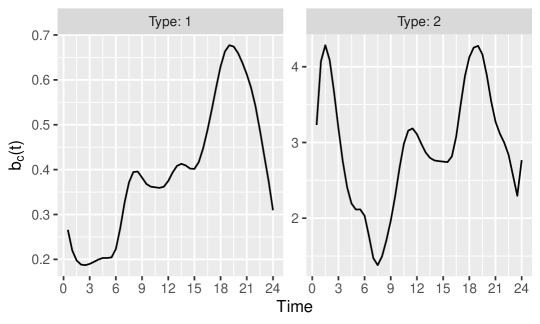
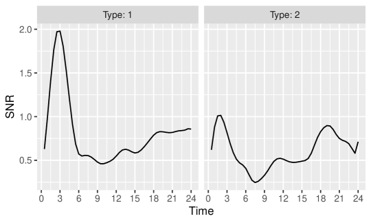
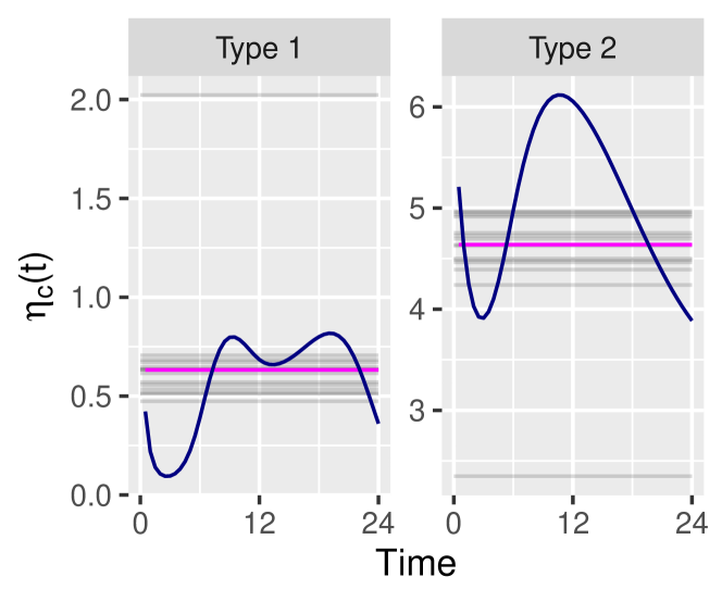
Figure 1 shows the baseline curves, the variance functionals and the signal-to-noise ratio (SNR) for each customer type. The SNR is simply the ratio of the typical curve to the variance functional at time . The baseline curves and variance functionals were based on the estimated typical curves obtained from the real data analysis in Section 4 of the main text. The type 1 baseline curve mimics the unrestricted domestic customer with lower consumption in early morning, increasing after 8 AM and reaching its peak at 8 PM. The Type 2 curve mimics the “Economy 7” customer with peaks around 2am and 8pm but with considerably larger electrical load values than Type 1. Customers variance functionals have higher values around the work period between 9am and 5pm, although Type 1 has two peaks that possibly represent when people leave from and arrive at their homes. The typical surfaces are shown in Figure 3.

The weather data containing temperature and air humidity were also based on real measurements for winter 2013 in Wales, United Kingdom. For this study, three sets of data were generated, representing three locations labelled T1, T2, and T3. Substations 1 to 4 were assigned to location T1, substations 5 to 8 to location T2, and the remaining substations 9 to 12 to location T3. Figure 2 shows the temperature and air humidity profiles for each location observed over 30 days. In fact, only data for scenarios 3, 4, 7, and 8 were generated in this manner. For scenarios 1, 2, 5, and 6, only the first five days were considered. In this study, temperature was used as the second component of the typical surface, and air humidity was used as an explanatory variable of the full aggregated data model with constant coefficient.

Furthermore, two explanatory variables were considered: air humidity as a functional variable, and a binary variable with value 1 for substations 1 and 2 and 0 otherwise, with associated coefficients and , respectively. Therefore, from Section 3.2 of the main paper, the full aggregated complete model can be written as
| (5) |
where is the dummy variable for substations 1 and 2 and the air humidity of substation at time of day . Finally, the true covariance decay parameters for each customer type were defined as and .


1.3.2 Results
In this study, for each of Scenarios 1 to 4 in Table 2, two models were fitted: one homogeneous and one complete aggregated data model. The homogeneous fit tests the performance of typical surface estimation under an under-parameterized covariance structure and the behaviour of the dispersion parameters by reducing the variance functional to a scalar. On the other hand, the complete model tests check whether, under the correct scenario, the proposed model performs well in terms of typical surface and covariance parameter estimation.
Throughout this section, the number of observed days and the market balance are explicitly shown to avoid consulting Table 2 to remember the scenario setup.
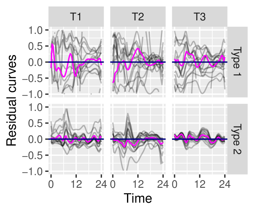
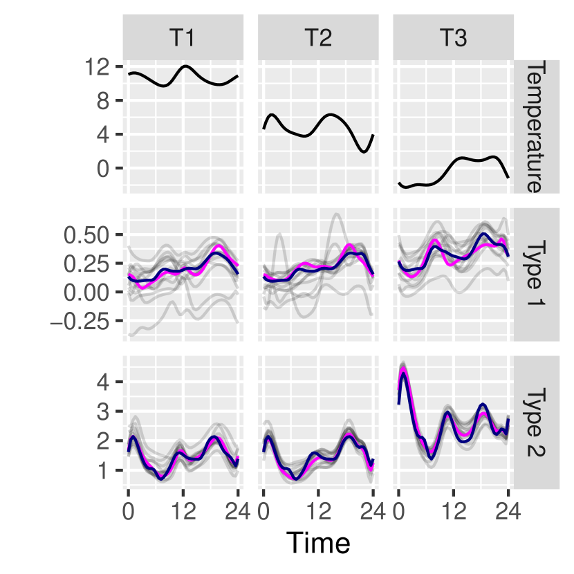
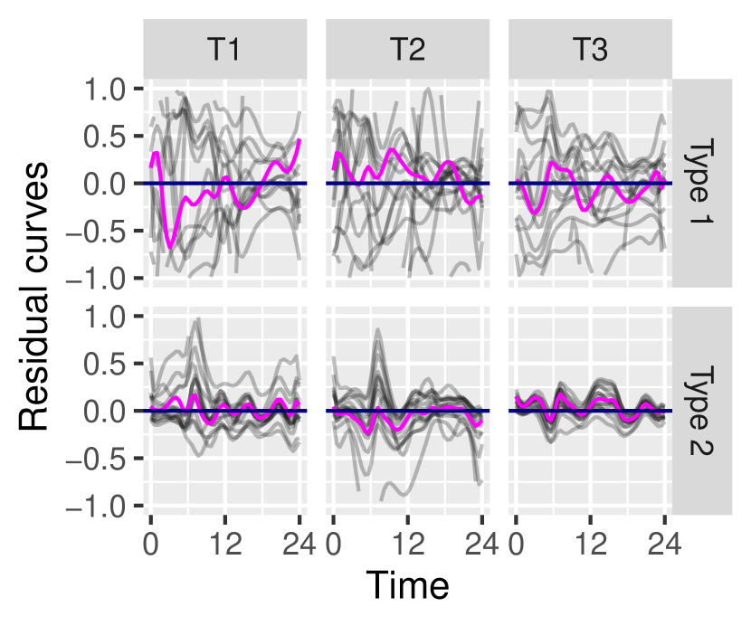
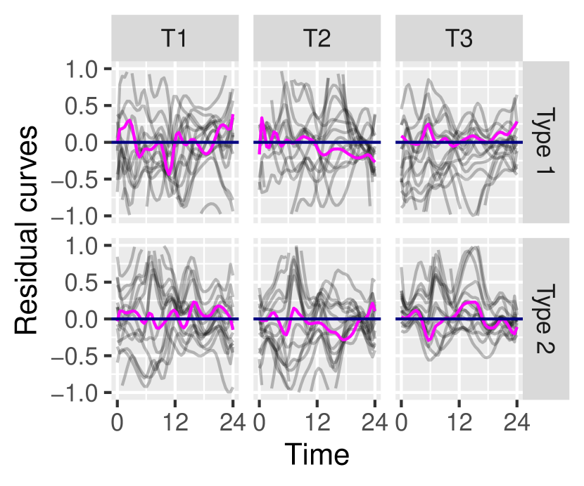
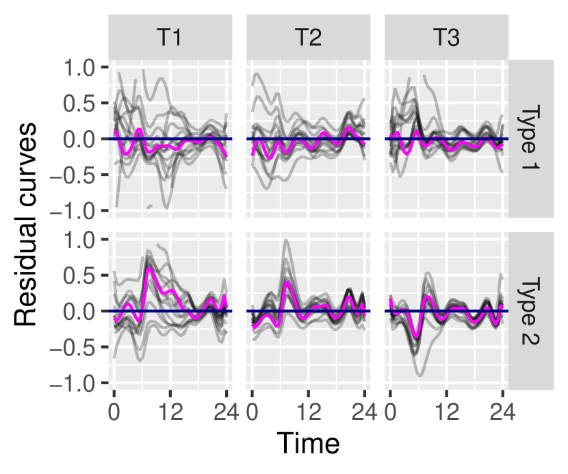
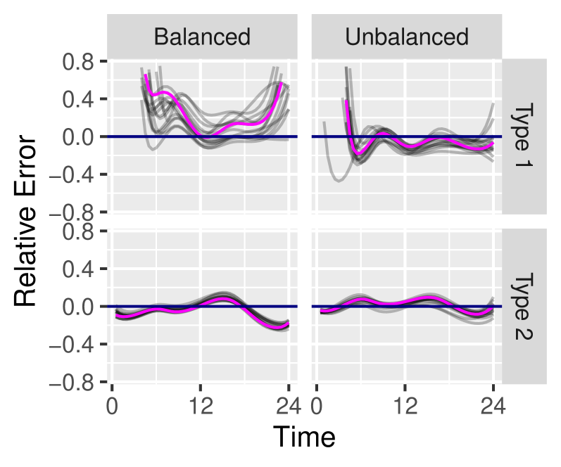
Starting with the homogeneous fit study, Figure 4 shows the estimated typical surfaces for some temperature curves for every combination of observed days and market balance. The first row in the panels represents a single instance of the temperature on the first observed day in the simulated data and in its respective primary group T1, T2 or T3. Observe that Figures 4a and 4b show estimated typical surfaces with noticeable variability, where some curves assume negative values. However, the balanced scenario in Figure 4a presents estimated curves for Type 2 with lower variability than those in Figure 4b. On the lower panels, Figures 4c and 4d show lower variability than the five-day scenarios. Furthermore, observe that the estimated curves for Type 2 in Figure 4c have even lower variability. In general, the median curves in the four scenarios show that the estimated curves are concentrated around their true values. This proximity to the true curve is better visualized in the residual curves shown in Figure 5. As presented in Section 1.1, these curves are standardized so that the scenario performance can be compared. Note that the residual curves for Type 2 in the five-day scenarios have lower variability in Figure 5a than their respective ones in Figure 5b, as mentioned earlier. The same event occurs in the 30-day scenarios, but with lower variability than the five-day scenarios. The four panels of Figure 5 show median curves oscillating around the horizontal zero-reference line, with no major differences among scenarios. To summarize the precision of the estimated typical surfaces shown in Figure 4, Table 3 shows the functional Mean Squared Relative Error for Scenarios 1 to 4 fitted by the homogeneous model. Clearly, the fMSRE for the estimated Type 1 typical curves is considerably higher in the five-day scenarios. It seems that the magnitude of the curves influences the variability of the estimates because the curves with greater magnitude in Type 2 have lower fMSRE than those with lower magnitude in Type 1. Moreover, all fMSRE for the 30-day scenarios are lower than the respective ones in the five-day scenarios.
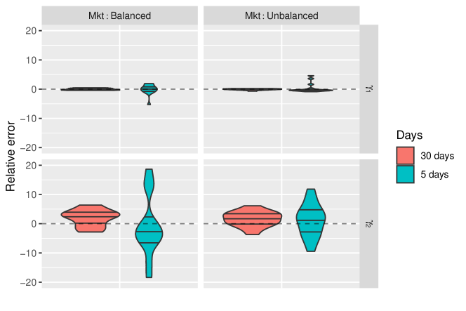
Figure 6a shows violin plots of the relative error of the estimated coefficients associated with the explanatory variables and . One run was excluded from the plot in the balanced scenario because it showed an absolute relative error greater than 38. In all scenarios, the estimates with have larger violins than those with . The 30-day scenarios have lower expected variability than the five-day scenario estimates, but their median reference lines above the zero line show visible underestimation of the parameter . Furthermore, Table 4 shows the mean, median and square root of the Mean Squared Relative Error (srMSRE) of the estimated parameters. Observe that parameter has estimates with considerably lower srMSRE than . The underestimation is notable in the mean and median values of . Nevertheless, the statistics of parameter show slight overestimation of the mean and larger srMSREs in all scenarios, especially the balanced five-day scenario, the one that presented a run with relative error greater than 38.
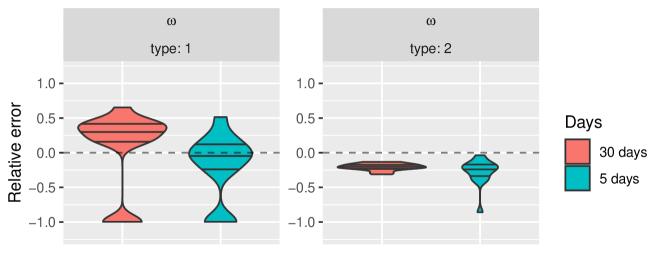
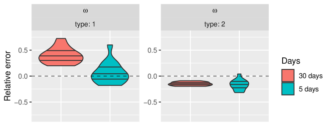
The estimated covariance parameters for Scenarios 1 to 4 are displayed in Figures 7 and 8 and Table 5. Figure 8 shows the estimated dispersion parameters represented over the true variance functionals, Figure 7 the violin plots of the estimated decay parameters and Table 5 the mean, median and square root of the Mean Squared Relative Error (MSRE)of the estimated decay parameters. Because the homogeneous model estimates a scalar as the dispersion parameter, the estimated values in Figure 8 are represented as constant lines over time. It seems that the horizontal lines are trying to capture an average of the variance functionals over time. In fact, taking the average of the variance functionals in Figure 8 over yields for Type 1 and for Type 2, which are close to the respective median lines at and . Moreover, the visibly overestimated valuefor Type 1 and the underestimated one for Type 2 in the unbalanced five-day scenario belong to the same run. On the other hand, the estimated decay parameters show systematic underestimation for Type 2 in all scenarios, as shown in Figure 7. The reduced estimate variability for the 30-day scenarios is observed only for estimated values of . Again, the difference in magnitude of the parameters seems to have an influence on their performance, because . Furthermore, Table 5 shows the underestimation of in the median and mean values and smaller srMSREs in favour of balanced markets in the five-day scenarios.
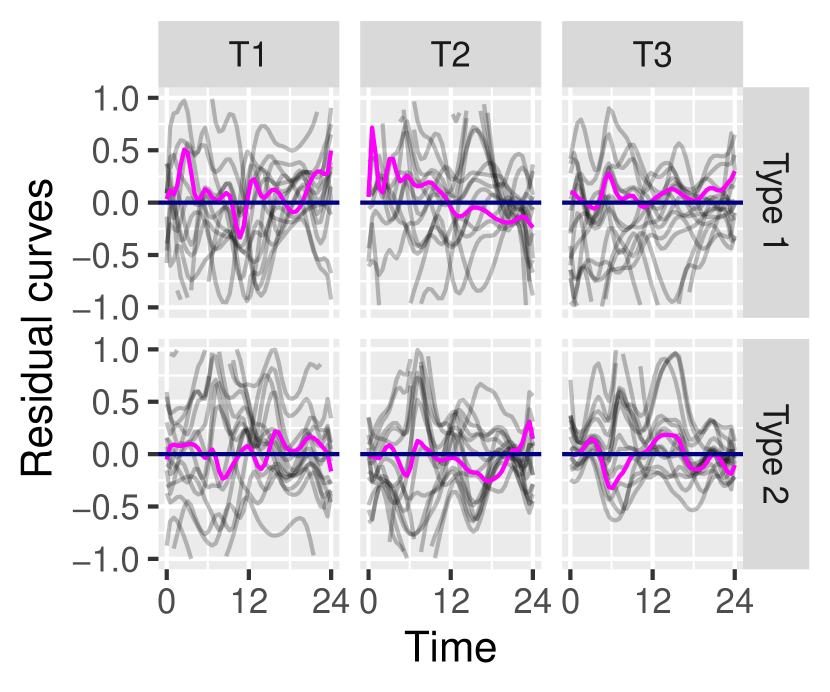
Figure 9 analogously shows the estimated typical surfaces for Scenarios 1 to 4 under the complete model fit. Again, observe that the estimated curve variability is reduced in the 30-day scenarios, especially for Type 2 under balanced markets. In addition, the advantage of balanced markets under the five-day scenarios can be seen from the lower variability of the residual curves in Figure 10 and the lower fMSRE in Table 3. The complete model does not present clear superiority in terms of fMSRE compared with the homogeneous model study.
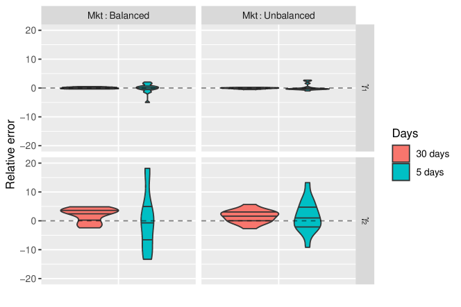
Figure 6b displays the relative errors of the estimated coefficients and associated with the explanatory variables. The characteristics of the violins are much like the respective ones in the homogeneous model. In fact, note that the srMSREs in Table 4 of both studies have similar values. Consequently, the complete model case shares the aspect of smaller srMSREs for estimates of , especially in the 30-day scenarios.
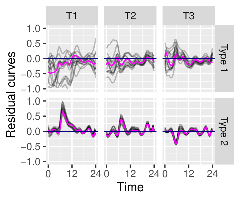
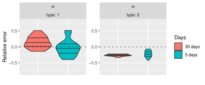
Finally, Figure 11 shows the estimated variance functionals of the complete model and Figure 12 their respective residual curves. As observed in the typical curves, the 30-day scenarios present lower estimate variability than the five-day scenarios. In general, the estimates capture the main features of the true curves, such as the prolonged higher values for customers of Type 1 and the decreasing values after 12 AM for Type 2. However, in some regions, the estimated curves present behaviour different from the true curve. In all scenarios, observe that the Type 1 curves begin almost at zero, whereas the true curve has a small peak with rapid decay. Moreover, in the balanced 30-day scenario, the estimated variance functionals for Type 2 customers present a nonexistent local peak at the end of the day. The violin plots of the relative errors of the estimated decay parameters are displayed in Figure 13 and their summary statistics in Table 5. Essentially, the complete model offers estimates with smaller srMSRE compared with the homogeneous model, but the underestimation of persists.
In addition, because the homogeneous model is nested in the complete model, Table LABEL:tab:simu-rvm in Section 1.5 shows the likelihood ratio test for all runs in every scenario. In all cases the test favours the complete model fit with p-values smaller than .


| Model | Days | Type | Market balance | fMSRE |
| Balanced | 17.6706 | |||
| Type 1 | Unbalanced | 18.4121 | ||
| Balanced | 0.8899 | |||
| 5 days | Type 2 | Unbalanced | 4.6557 | |
| Balanced | 1.9525 | |||
| Type 1 | Unbalanced | 2.1867 | ||
| Balanced | 0.5814 | |||
| Homogeneous | 30 days | Type 2 | Unbalanced | 1.0923 |
| Balanced | 19.5322 | |||
| Type 1 | Unbalanced | 14.9073 | ||
| Balanced | 0.9747 | |||
| 5 days | Type 2 | Unbalanced | 3.9616 | |
| Balanced | 1.9122 | |||
| Type 1 | Unbalanced | 1.9651 | ||
| Balanced | 0.7720 | |||
| Complete | 30 days | Type 2 | Unbalanced | 1.1850 |
| Model | Parameter | Days | Market | Mean | Median | |
| Balanced | 12.7193 | 12.0985 | 0.3054 | |||
| 30 days | Unbalanced | 11.8776 | 12.1702 | 0.2516 | ||
| Balanced | 12.0501 | 12.1832 | 1.7045 | |||
| 5 days | Unbalanced | 17.2909 | 8.3669 | 1.6263 | ||
| Balanced | 0.0330 | 0.0421 | 3.4016 | |||
| 30 days | Unbalanced | 0.0289 | 0.0328 | 2.9574 | ||
| Balanced | 0.0156 | -0.0159 | 14.6551 | |||
| Homogeneous | 5 days | Unbalanced | 0.0231 | 0.0334 | 5.6259 | |
| Balanced | 13.3503 | 12.9929 | 0.2578 | |||
| 30 days | Unbalanced | 11.8177 | 12.1773 | 0.2295 | ||
| Balanced | 11.3529 | 15.1660 | 1.6096 | |||
| 5 days | Unbalanced | 15.3926 | 9.1294 | 1.1091 | ||
| Balanced | 0.0330 | 0.0490 | 3.0979 | |||
| 30 days | Unbalanced | 0.0283 | 0.0337 | 2.5957 | ||
| Balanced | 0.0254 | 0.0104 | 15.3070 | |||
| Complete | 5 days | Unbalanced | 0.0274 | 0.0264 | 5.4715 |


| Model | Parameter | Days | Market | Median | Mean | |
| Balanced | 0.0257 | 0.0275 | 0.2549 | |||
| 30 days | Unbalanced | 0.0382 | 0.0322 | 0.5544 | ||
| Balanced | 0.0270 | 0.0259 | 0.2107 | |||
| 5 days | Unbalanced | 0.0287 | 0.0764 | 6.6934 | ||
| Balanced | 0.5028 | 0.5079 | 0.2764 | |||
| 30 days | Unbalanced | 0.5520 | 0.5562 | 0.2111 | ||
| Balanced | 0.5226 | 0.5251 | 0.2675 | |||
| Homogeneous | 5 days | Unbalanced | 0.5427 | 0.5073 | 0.3318 | |
| Balanced | 0.0316 | 0.0298 | 0.4243 | |||
| 30 days | Unbalanced | 0.0419 | 0.0418 | 0.4208 | ||
| Balanced | 0.0288 | 0.0291 | 0.2516 | |||
| 5 days | Unbalanced | 0.0312 | 0.0318 | 0.2065 | ||
| Balanced | 0.5169 | 0.5178 | 0.2621 | |||
| 30 days | Unbalanced | 0.5899 | 0.5962 | 0.1521 | ||
| Balanced | 0.5323 | 0.5450 | 0.2418 | |||
| Complete | 5 days | Unbalanced | 0.5819 | 0.5831 | 0.1917 |


1.3.3 Discussion and conclusion
In all scenarios, the estimated typical surfaces of the homogeneous model are robust to the misspecification of the covariance structure, as shown in Figure 4. Both studies show an expected better performance for the 30-day scenarios in terms of estimation variability and fMSRE, which is also true for balanced scenarios compared to unbalanced ones.
Interestingly, it seems that the magnitude of the parameters may influence the quality of the estimate. The estimated typical curves, for example, show better estimates for customers of Type 2, the ones with higher consumption curves compared to Type 1. The same characteristic is observed in the relative errors of the estimates of , a parameter much greater than . Nonetheless, this is not as evident in the decay parameter estimation. The latter seems to be especially difficult to estimate because its performance in terms of precision and srMSRE (square root of the mean squared relative error) is not improved under 30-day scenarios or balanced markets. In fact, the estimates present a systematic underestimation of . Still on the covariance structure, the estimated variance functionals in the complete study can capture the main features of the true ones, despite an unexpected local peak in the 30-day scenario with balanced market.
In general, the advantages of balanced markets and 30-day scenarios is evident. The complete model provides a functional variance structure that can capture different dispersions over time. However, in terms of typical surface estimation, there is no clear difference between the homogeneous and the complete model fit, which could be attributed to the fact that the least-squares estimators are unbiased independently of the covariance structure, as noted in Section 3.6 of the main text.
1.4 Clustering the aggregated model
This section studies the clustering approach of the aggregated data model presented in Section 3.5 of the main manuscript. The method was tested in Scenarios 5 to 8 and is presented in Table 2, where data from three clusters were simulated under the homogeneous covariance structure. In contrast to Section 1.3, typical surfaces were not considered here for the clustering model.
Section 1.4.1 details the clustering configuration and the true parameters. Sections 1.4.2 describes the main results and 1.4.3 contains the discussion and conclusions of this simulation study.
1.4.1 Clustering setup and true parameters
Scenarios 5 to 8 in Table 2 are made up of variations of the number of days (5 and 30) and the market (balanced and unbalanced). The remaining simulation parameters were fixed to three clusters and two types of customers observed in 12 substations every 30 minutes. The true cluster allocation is displayed in Table 6, where substations 1 to 6 are assigned to Cluster 1, substations 7 to 10 to Cluster 2 and finally substations 11 and 12 to Cluster 3. The chosen covariance structure is the homogeneous one, where each customer type has its own dispersion and decay parameters.
| Substation | 1 | 2 | 3 | 4 | 5 | 6 | 7 | 8 | 9 | 10 | 11 | 12 |
| True cluster | 1 | 1 | 1 | 1 | 1 | 1 | 2 | 2 | 2 | 2 | 3 | 3 |

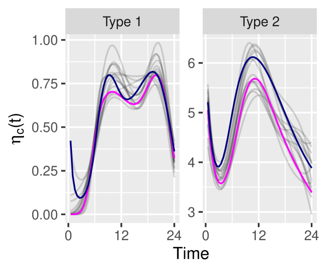
Figure 14 shows the six typical curves divided into the two customer types for each of the three clusters. Their shapes were based on the estimated typical curves for the UK energy grid dataset in Section 4.3 of the main paper. Hence, Type 1 mimics the unrestricted domestic customer, with similar shapes among clusters, whereas Type 2 mimics the “Economy 7” customer.
The covariance parameters that compose the homogeneous covariance structure of the simulated scenarios are presented in Table 7 divided by cluster, parameter and customer type, where, again, their values were based on the estimated covariance parameters for the UK energy grid dataset described in Section 4.3 of the main manuscript.
| Cluster | Parameter | Type | Value |
| 1.54 | |||
| 1.53 | |||
| 0.16 | |||
| 0.03 | |||
| 1.07 | |||
| 1.28 | |||
| 0.12 | |||
| 0.09 | |||
| 0.43 | |||
| 5.18 | |||
| 0.02 | |||
| 0.37 |
1.4.2 Results
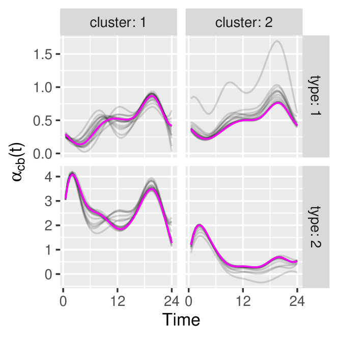
Scenarios 5 to 8 were subjected to two model fits: clustering homogeneous aggregated data models with two and three clusters. The two-cluster fit tested how the model would perform if the number of clusters were underdetermined, that is, how the method groups substations and consequently what are the characteristics of the estimated typical curves and covariance parameters. On the other hand, the three-cluster fit evaluates model performance under correct scenarios.
Before presenting the results, it is necessary to note the number of runs that did not converge or converged to a local maximum in this simulation at each model fit. The non-convergent runs in the two-cluster fit were the following: two runs in the unbalanced five-day market scenario, one run in the balanced five-day market scenario, and two runs in the balanced 30-day market scenario. Moreover, the three-cluster fit had three non-convergent runs in both balanced and unbalanced five-day market scenarios, four in the unbalanced 30-day scenario, and two in the balanced 30-day scenarios. The runs that converged to local maxima presented anomalous estimated typical curves with negative and discrepant values.
Let us begin with the two-cluster fit and its respective substation clustering as shown in Table 8. In all runs, substations are assigned with high probability to the same cluster configuration, and therefore Substations 1 to 6 were assigned to Cluster 1, Substations 7 to 10 to Cluster 2, and Substations 11 and 12 to Cluster 3. Note that the substations of true Cluster 3 were assigned to the larger Cluster 1 in the two-cluster model. Recall also that the true Clusters 1 and 3 in Figure 14 have similar typical curves for Type 1 and Type 2 and that both have approximately the same magnitude and characteristics over time, and hence it is reasonable that they merge into a single cluster in the two-cluster model.
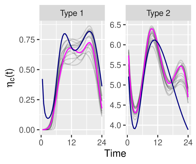
Figure 15 shows the estimated typical curves for Scenarios 5 to 8 under the two- cluster model fit. In general, observe that Cluster 1 curves capture the main characteristics of Clusters 1 and 3: the work period stability, the 8 PM peak of Type 1 curves, and the 2 AM and 8 PM peaks of Type 2 curves. The 30-day scenarios have slightly lower estimate variability than the five-day scenarios, but note that the Type 2 curves in Cluster 1 have runs with different estimated characteristics of the work period, as shown in Figures 15c and 15d. In fact, the main difference between true Clusters 1 and 3 is the work period characterization of Type 2, and therefore it is to be expected that some runs could estimate typical curves in favour of the true Cluster 1 or Cluster 3.
Table 9 shows the summary statistics of the estimated covariance parameters of the two-cluster model fit. Because the estimated Cluster 2 substations coincide with the substations in the true Cluster 2, it is to be expected that their estimated covariance parameters are close to their true values. Observe in Table 9that the median and mean of the estimated parameters for Cluster 2 are close to their true values in the Reference column, especially for 30-day scenarios. Under five-day scenarios, balanced markets have better estimates in terms of precision. On the other hand, Cluster 1 estimates are located between the true values of true Clusters 1 and 3, and therefore the Reference column for Cluster 1 in Table 9 represents the mean of the covariance parameters of the true Clusters 1 and 3. The proximity of estimated and true covariance parameters is greater for customers of Type 2. In contrast, the Type 2 true dispersion parameters of Clusters 1 and 3 present the largest difference in Table 7, 1.54 and 5.18 respectively. Nonetheless, there is no clear evidence that the estimated covariance parameters in Cluster 1 are close to the average of the true parameters of Clusters 1 and 3.
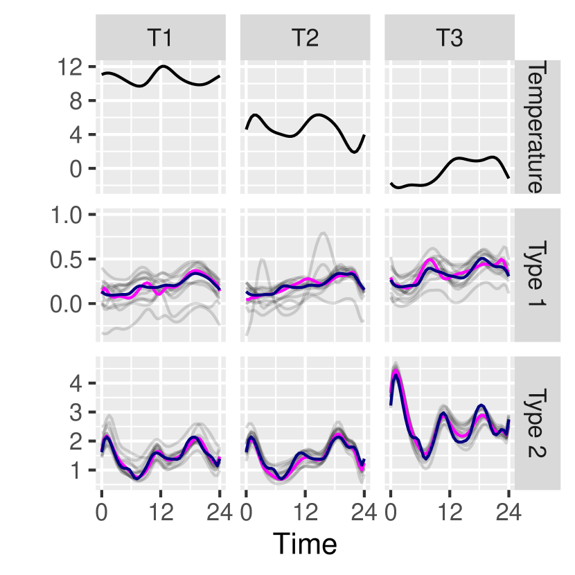
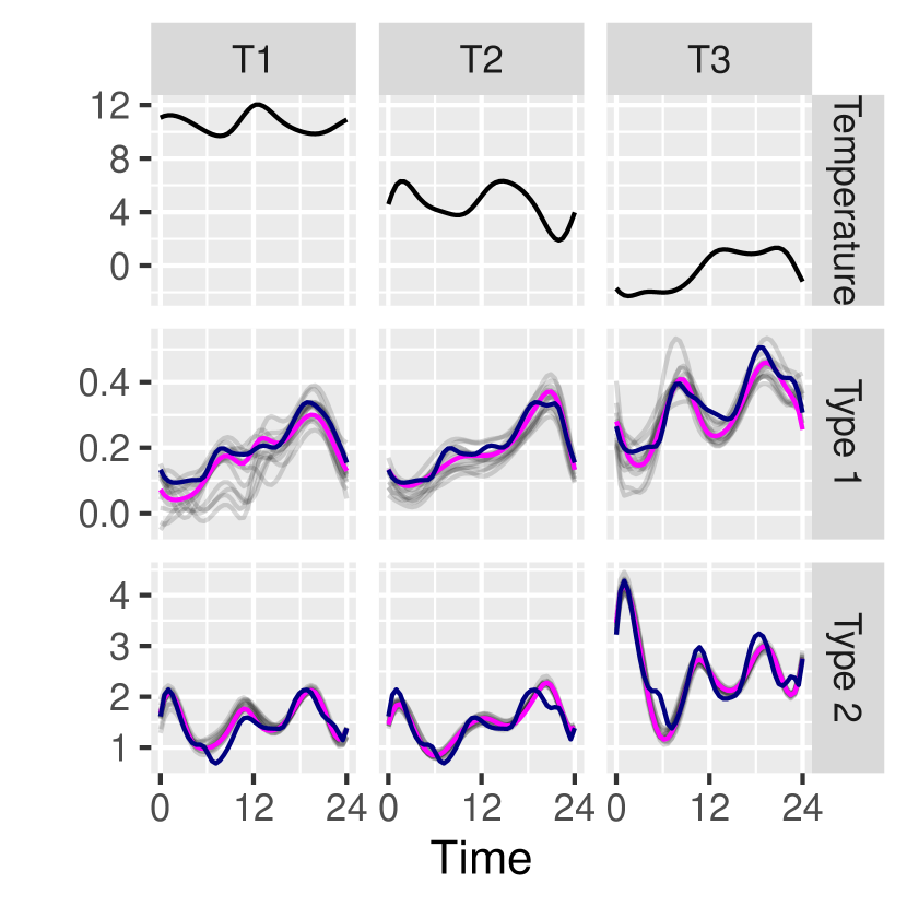
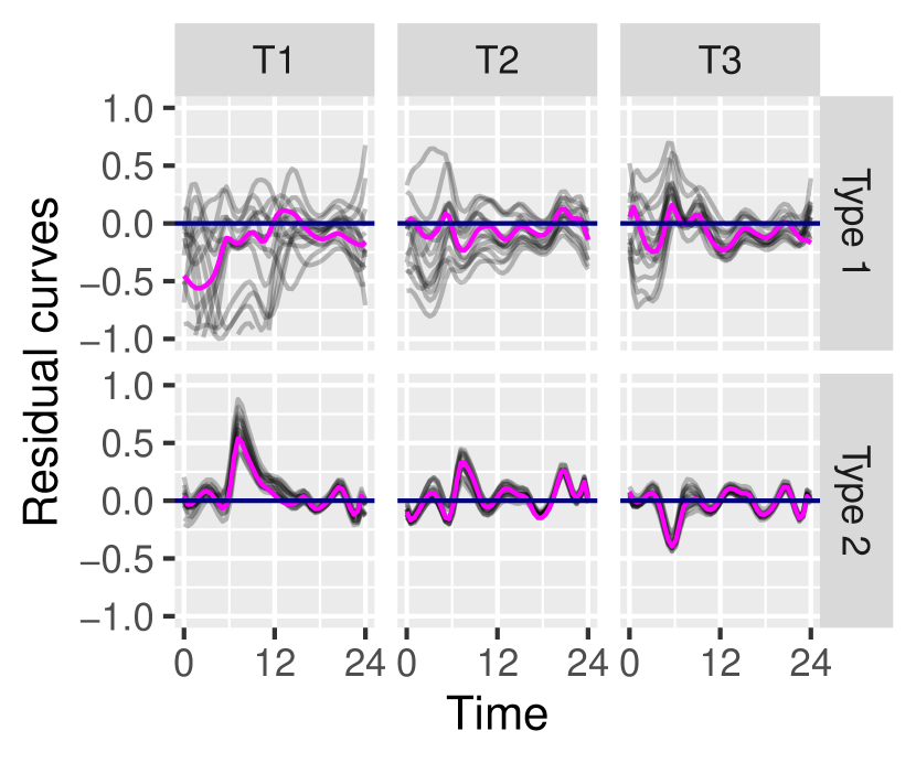
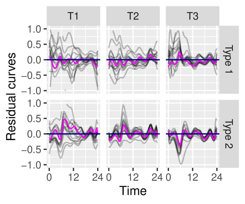
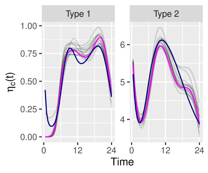
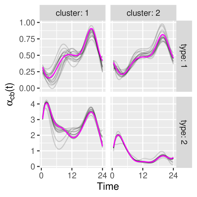
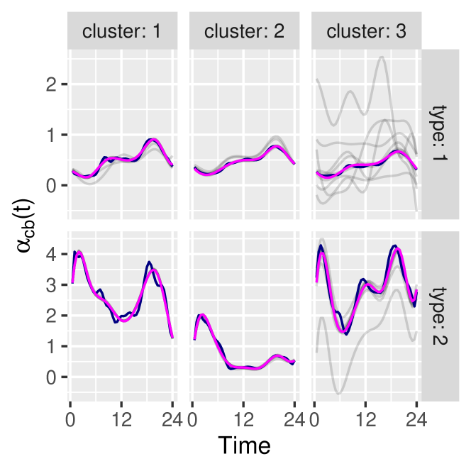
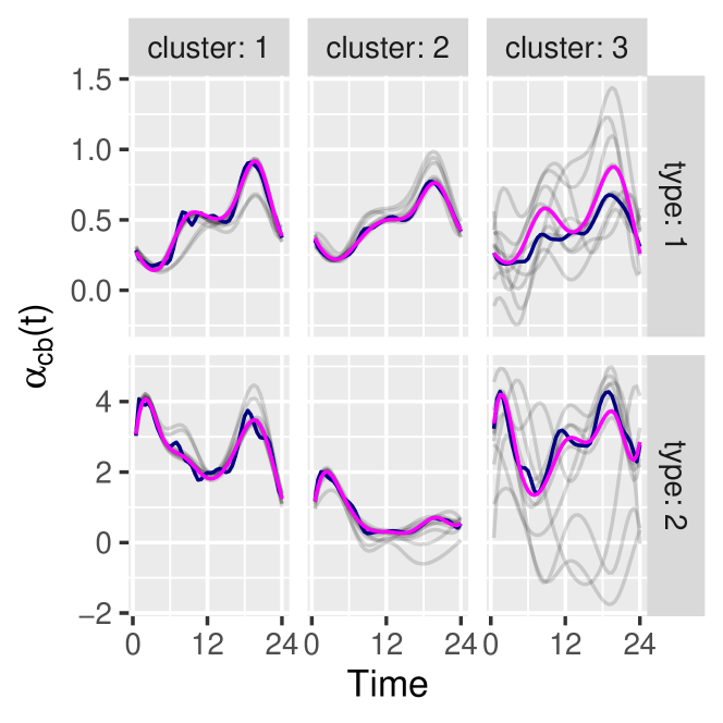
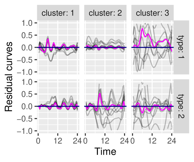
The estimated typical curves of the three-cluster model are displayed in Figure 16 and their associated residual curves in Figure 17. In general, the median curves show that the estimated curves capture the main characteristics of the true typical curves, although there are visible discrepant examples, more frequently seen in the unbalanced scenarios, as shown in Figures 16b and 16c. Negative values could be avoided by restricting the typical curve estimation, but to avoid overextending the computational burden of this simulation, it was decided to retain the least-squares estimators in exchange for some negative values, and also to show that in general the estimator is robust for different scenarios because the median curves are positive along the entire time axis. Once more, the residual curves show that the 30-day scenarios are more concentrated around the zero-reference line than the five-day scenarios, with even better fits for balanced scenarios. In this clustering approach, the relative residual curves for Cluster 3 in the unbalanced scenario do not concentrate around the zero-reference line, as shown in Figures 17b and 17d. Furthermore, Cluster 1 has residual curves with lower variability than Cluster 3 in all scenarios. In fact, Cluster 1 contains six substations, whereas Cluster 3 contains two substations, the minimum number required for model identifiability. It seems that the larger the number of substations in the cluster, the better is the precision, and consequently this might be the reason for the Cluster 3 overestimation of the typical curves, particularly under unbalanced scenarios.
The estimated covariance parameters of the three-cluster models are represented by their mean, median and srMSRE in Table LABEL:tab:simu-cl3-tab. As observed in previous results throughout this section, smallest srMSRE are associated with parameters with larger magnitudes, for example, and . n contrast, the largest srMSRE are associated with parameters with smaller magnitudes, for example, . In the latter case, the unbalanced scenarios presented smaller srMSRE than the balanced markets. In cases like , increasing the number of observation days from 5 to 30 improved srMSRE. The same behaviour was observed in most parameters, particularly those with small magnitude. On the other hand, parameters and were the smallest parameters in the simulation, but the srMSREs of were mostly around 1.5, whereas the srMSREs of had three values greater than 10. Recall that Cluster 3 contained only two substations. Therefore, as mentioned earlier for typical curve estimation, both the number of substations and the number of observation days are important to improve parameter estimation in each cluster.
To avoid an overextended table in this section, the comparison of BIC values between the two- and three-cluster models is presented in Table LABEL:tab:simu-bic in Section 1.5. In all cases, the BIC is favourable to the three-cluster model with differences mostly of order .


| Substation | True | two-cluster fit | three-cluster fit |
| 1 | 1 | 1 | 1 |
| 2 | 1 | 1 | 1 |
| 3 | 1 | 1 | 1 |
| 4 | 1 | 1 | 1 |
| 5 | 1 | 1 | 1 |
| 6 | 1 | 1 | 1 |
| 7 | 2 | 2 | 2 |
| 8 | 2 | 2 | 2 |
| 9 | 2 | 2 | 2 |
| 10 | 2 | 2 | 2 |
| 11 | 3 | 1 | 3 |
| 12 | 3 | 1 | 3 |
| Parameter | Days | Market | Ref | Median | Mean | Std Dev |
| Balanced | 0.985 | 1.3690 | 1.1717 | 0.6952 | ||
| 30 days | Unbalanced | 0.985 | 1.4175 | 1.4324 | 0.1123 | |
| Balanced | 0.985 | 1.2360 | 1.0226 | 0.5916 | ||
| 5 days | Unbalanced | 0.985 | 1.3903 | 0.9552 | 0.7257 | |
| Balanced | 0.090 | 0.1863 | 1.7907 | 3.2170 | ||
| 30 days | Unbalanced | 0.090 | 0.1303 | 0.1457 | 0.0323 | |
| Balanced | 0.090 | 0.2262 | 2.4892 | 3.6509 | ||
| 5 days | Unbalanced | 0.090 | 0.4885 | 1.7235 | 2.2490 | |
| Balanced | 3.355 | 3.3149 | 3.7087 | 1.0352 | ||
| 30 days | Unbalanced | 3.355 | 3.8129 | 3.3212 | 0.7789 | |
| Balanced | 3.355 | 4.0515 | 4.0523 | 0.7751 | ||
| 5 days | Unbalanced | 3.355 | 3.7831 | 4.1194 | 0.9537 | |
| Balanced | 0.200 | 0.1247 | 0.1559 | 0.0653 | ||
| 30 days | Unbalanced | 0.200 | 0.1859 | 0.1728 | 0.0768 | |
| Balanced | 0.200 | 0.1983 | 0.1848 | 0.0644 | ||
| 5 days | Unbalanced | 0.200 | 0.2595 | 0.2048 | 0.0891 | |
| Balanced | 1.070 | 1.1663 | 1.2281 | 0.3476 | ||
| 30 days | Unbalanced | 1.070 | 1.0870 | 1.1621 | 0.1524 | |
| Balanced | 1.070 | 1.0906 | 1.1274 | 0.3569 | ||
| 5 days | Unbalanced | 1.070 | 1.2591 | 1.1776 | 0.3398 | |
| Balanced | 0.120 | 0.1290 | 0.3108 | 0.7708 | ||
| 30 days | Unbalanced | 0.120 | 0.1143 | 0.1152 | 0.0071 | |
| Balanced | 0.120 | 0.1080 | 0.3592 | 1.0368 | ||
| 5 days | Unbalanced | 0.120 | 0.1134 | 1.0093 | 2.3378 | |
| Balanced | 1.280 | 1.4533 | 1.3147 | 0.3727 | ||
| 30 days | Unbalanced | 1.280 | 1.3541 | 1.2999 | 0.8166 | |
| Balanced | 1.280 | 1.4583 | 0.9738 | 0.7445 | ||
| 5 days | Unbalanced | 1.280 | 0.3949 | 0.8713 | 1.0385 | |
| Balanced | 0.090 | 0.0958 | 0.3894 | 0.8949 | ||
| 30 days | Unbalanced | 0.090 | 0.1233 | 1.4038 | 2.7188 | |
| Balanced | 0.090 | 0.0998 | 2.2790 | 3.1786 | ||
| 5 days | Unbalanced | 0.090 | 3.6099 | 4.7933 | 4.9760 |


| Parameter | Days | Market | Median | Mean | |
|---|---|---|---|---|---|
| Balanced | 1.0862 | 1.0114 | 0.6470 | ||
| 30 days | Unbalanced | 1.3929 | 1.2079 | 0.4677 | |
| Balanced | 0.9430 | 0.8281 | 0.6991 | ||
| 5 days | Unbalanced | 1.3859 | 1.2022 | 0.4923 | |
| Balanced | 0.3220 | 2.2018 | 3.5878 | ||
| 30 days | Unbalanced | 0.1295 | 0.3441 | 1.1971 | |
| Balanced | 3.9317 | 6.5328 | 6.3132 | ||
| 5 days | Unbalanced | 0.1274 | 0.9780 | 2.3491 | |
| Balanced | 2.8842 | 2.9041 | 0.9477 | ||
| 30 days | Unbalanced | 2.7891 | 2.8831 | 0.9404 | |
| Balanced | 2.8640 | 2.9372 | 0.9590 | ||
| 5 days | Unbalanced | 2.7464 | 2.7632 | 0.9386 | |
| Balanced | 0.0759 | 0.0777 | 1.2608 | ||
| 30 days | Unbalanced | 0.0960 | 0.0985 | 1.5111 | |
| Balanced | 0.0736 | 0.0807 | 1.3000 | ||
| 5 days | Unbalanced | 0.1057 | 0.4043 | 3.5322 | |
| Balanced | 1.0274 | 1.0346 | 0.4578 | ||
| 30 days | Unbalanced | 1.0810 | 1.1472 | 0.3197 | |
| Balanced | 0.6081 | 0.6888 | 0.7774 | ||
| 5 days | Unbalanced | 1.2345 | 1.2259 | 0.4379 | |
| Balanced | 0.1208 | 0.6763 | 2.1698 | ||
| 30 days | Unbalanced | 0.1226 | 0.1344 | 0.4184 | |
| Balanced | 1.4476 | 2.4465 | 4.4133 | ||
| 5 days | Unbalanced | 0.1083 | 0.5807 | 2.0123 | |
| Balanced | 1.5417 | 1.5858 | 0.4888 | ||
| 30 days | Unbalanced | 1.2823 | 1.2391 | 0.4312 | |
| Balanced | 1.5092 | 1.5814 | 0.4852 | ||
| 5 days | Unbalanced | 0.0363 | 0.5207 | 0.9565 | |
| Balanced | 0.0960 | 0.0965 | 0.2692 | ||
| 30 days | Unbalanced | 0.1057 | 0.4156 | 1.9330 | |
| Balanced | 0.0877 | 0.0884 | 0.2444 | ||
| 5 days | Unbalanced | 5.2492 | 5.6967 | 7.8929 | |
| Balanced | 0.3390 | 1.4096 | 1.7326 | ||
| 30 days | Unbalanced | 1.3438 | 1.4685 | 1.5540 | |
| Balanced | 0.0282 | 0.4760 | 1.1353 | ||
| 5 days | Unbalanced | 1.0871 | 1.0075 | 1.3569 | |
| Balanced | 3.9775 | 3.2759 | 12.7591 | ||
| 30 days | Unbalanced | 0.1446 | 0.3754 | 4.2157 | |
| Balanced | 9.9767 | 10.3302 | 22.7049 | ||
| 5 days | Unbalanced | 0.9252 | 2.7126 | 11.6030 | |
| Balanced | 5.2455 | 5.0097 | 0.3249 | ||
| 30 days | Unbalanced | 3.9596 | 3.3274 | 0.5980 | |
| Balanced | 4.7792 | 4.6787 | 0.3502 | ||
| 5 days | Unbalanced | 4.0859 | 3.9616 | 0.4917 | |
| Balanced | 0.2624 | 0.2492 | 0.5713 | ||
| 30 days | Unbalanced | 0.2968 | 0.6871 | 1.1099 | |
| Balanced | 0.1930 | 0.1960 | 0.6859 | ||
| 5 days | Unbalanced | 0.2759 | 0.8170 | 1.3016 |
1.4.3 Discussion and conclusion
In both fitted models, substations are allocated to the same clusters throughout the series of runs. In the two-cluster model, Substations 11 and 12, which belong to the true Cluster 3, are always assigned to Cluster 1 together with Substations 1 to 6. In this case, with an underdetermined number of clusters, the method groups the clusters with more similarity. Hence the estimated typical curves for Cluster 1 still capture the main features of the true curves for Clusters 1 and 3. Similarly, the estimated covariance parameters for Cluster 1 present values between the true covariance parameters of the true Clusters 1 and 3. In the three-cluster model, substations are assigned to the correct cluster. Consequently, except for some cases under unbalanced scenarios, estimated typical curves for this model are well located around their true curves. In general, 30-day scenarios have less dispersed estimates than five-day scenarios, and balanced markets have less dispersed estimates than unbalanced ones.
The differences among scenarios have a similar impact on the estimation of covariance parameters. In addition, there is evidence that the number of substations in a cluster is crucial to estimation performance, particularly for small-magnitude parameters. The positive impact of increasing the number of substations on parameter estimation is shown in Lenzi et al. (2017). Two parameters with small values for Clusters 1 and 3 have distinct srMSRE probably because the information available for Cluster 3 estimation is less than for Cluster 1.
When comparing both models, the three-cluster model presents lower BIC than the two-cluster model in all cases.In a real-world problem, where the true number of clusters is unknown, the BIC can be a useful tool to decide between models.
Users of the clustering aggregated data model are encouraged to be careful with the estimated covariance parameters and to try multiple models with different numbers of clusters using these estimated values as input for their initial values. For example, the estimated values of the aggregated two-cluster data model can be used as an input to fit the aggregated three-cluster data model by repeating one of the results. As shown in Section 2.5, after multiple fits, the user can compare the models using the likelihood test ratio to help decide which model is the most adequate to the data.
1.5 Additional tables
| Log-likelihood | |||||
| Days | Run | Homogeneous | Complete | Test statistic | p-value |
| 5 days | 1 | 11356.44 | 11206.11 | 300.6677 | <0.0001 |
| 5 days | 2 | 11468.83 | 11279.91 | 377.8489 | <0.0001 |
| 5 days | 3 | 11329.26 | 11129.60 | 399.3154 | <0.0001 |
| 5 days | 4 | 11393.79 | 11237.21 | 313.1679 | <0.0001 |
| 5 days | 5 | 11380.05 | 11161.95 | 436.2019 | <0.0001 |
| 5 days | 6 | 11412.08 | 11240.27 | 343.6055 | <0.0001 |
| 5 days | 7 | 11409.96 | 11230.16 | 359.5910 | <0.0001 |
| 5 days | 8 | 11380.91 | 11221.02 | 319.7964 | <0.0001 |
| 5 days | 9 | 11296.43 | 11111.48 | 369.8967 | <0.0001 |
| 5 days | 10 | 11293.50 | 11131.60 | 323.7867 | <0.0001 |
| 5 days | 11 | 11297.66 | 11132.56 | 330.1824 | <0.0001 |
| 5 days | 12 | 11380.86 | 11204.74 | 352.2391 | <0.0001 |
| 5 days | 13 | 11305.42 | 11135.14 | 340.5573 | <0.0001 |
| 5 days | 14 | 11357.41 | 11182.27 | 350.2775 | <0.0001 |
| 5 days | 15 | 11337.32 | 11153.20 | 368.2447 | <0.0001 |
| 5 days | 16 | 12252.88 | 12167.35 | 171.0486 | <0.0001 |
| 5 days | 17 | 12199.07 | 12079.56 | 239.0298 | <0.0001 |
| 5 days | 18 | 12315.08 | 12222.54 | 185.0706 | <0.0001 |
| 5 days | 19 | 12394.19 | 12316.81 | 154.7764 | <0.0001 |
| 5 days | 20 | 12254.24 | 12160.62 | 187.2429 | <0.0001 |
| 5 days | 21 | 12286.01 | 12189.36 | 193.3048 | <0.0001 |
| 5 days | 22 | 12314.49 | 12225.54 | 177.8949 | <0.0001 |
| 5 days | 23 | 12173.57 | 12073.10 | 200.9313 | <0.0001 |
| 5 days | 24 | 12248.57 | 12150.72 | 195.6961 | <0.0001 |
| 5 days | 25 | 12197.71 | 12090.13 | 215.1580 | <0.0001 |
| 5 days | 26 | 12304.61 | 12196.86 | 215.4922 | <0.0001 |
| 5 days | 27 | 12135.35 | 12034.37 | 201.9598 | <0.0001 |
| 5 days | 28 | 12385.44 | 12302.31 | 166.2589 | <0.0001 |
| 5 days | 29 | 12359.07 | 12253.33 | 211.4677 | <0.0001 |
| 5 days | 30 | 12249.15 | 12142.30 | 213.7031 | <0.0001 |
| 30 days | 1 | 68412.15 | 67418.28 | 1987.7512 | <0.0001 |
| 30 days | 2 | 68555.41 | 67692.07 | 1726.6639 | <0.0001 |
| 30 days | 3 | 68409.85 | 67507.56 | 1804.5693 | <0.0001 |
| 30 days | 4 | 68848.74 | 67854.20 | 1989.0811 | <0.0001 |
| 30 days | 5 | 68853.23 | 67912.53 | 1881.3950 | <0.0001 |
| 30 days | 6 | 68254.05 | 67181.14 | 2145.8196 | <0.0001 |
| 30 days | 7 | 68428.22 | 67442.46 | 1971.5111 | <0.0001 |
| 30 days | 8 | 68720.86 | 67794.68 | 1852.3555 | <0.0001 |
| 30 days | 9 | 68143.11 | 67241.85 | 1802.5107 | <0.0001 |
| 30 days | 10 | 68639.51 | 67645.38 | 1988.2693 | <0.0001 |
| 30 days | 11 | 68532.07 | 67568.32 | 1927.5025 | <0.0001 |
| 30 days | 12 | 68452.58 | 67430.66 | 2043.8409 | <0.0001 |
| 30 days | 13 | 68697.84 | 67687.06 | 2021.5609 | <0.0001 |
| 30 days | 14 | 68183.63 | 67221.51 | 1924.2479 | <0.0001 |
| 30 days | 15 | 68828.41 | 67972.03 | 1712.7790 | <0.0001 |
| 30 days | 16 | 73834.91 | 73325.45 | 1018.9162 | <0.0001 |
| 30 days | 17 | 74309.19 | 73894.94 | 828.4990 | <0.0001 |
| 30 days | 18 | 74396.67 | 73964.25 | 864.8214 | <0.0001 |
| 30 days | 19 | 74607.51 | 74136.77 | 941.4789 | <0.0001 |
| 30 days | 20 | 74741.17 | 74284.07 | 914.1883 | <0.0001 |
| 30 days | 21 | 74686.06 | 74273.96 | 824.1941 | <0.0001 |
| 30 days | 22 | 74678.44 | 74242.28 | 872.3236 | <0.0001 |
| 30 days | 23 | 74295.85 | 73798.20 | 995.2966 | <0.0001 |
| 30 days | 24 | 73439.84 | 72817.88 | 1243.9196 | <0.0001 |
| 30 days | 25 | 74510.71 | 74113.48 | 794.4602 | <0.0001 |
| 30 days | 26 | 74232.01 | 73790.03 | 883.9603 | <0.0001 |
| 30 days | 27 | 74783.54 | 74378.31 | 810.4463 | <0.0001 |
| 30 days | 28 | 74510.23 | 74068.60 | 883.2588 | <0.0001 |
| 30 days | 29 | 74963.07 | 74588.12 | 749.8957 | <0.0001 |
| 30 days | 30 | 74913.23 | 74506.08 | 814.3098 | <0.0001 |
| BIC | ||||
| Days | Run | 2 Clusters | 3 Clusters | BIC diff |
| 5 days | 1 | 22892.98 | 22653.75 | 239.24 |
| 5 days | 2 | 23037.71 | 22728.32 | 309.38 |
| 5 days | 3 | 22765.23 | 22522.55 | 242.68 |
| 5 days | 4 | 23002.98 | 22632.54 | 370.44 |
| 5 days | 5 | NA | NA | NA |
| 5 days | 6 | 22867.82 | 22589.01 | 278.82 |
| 5 days | 7 | 22928.48 | 22674.78 | 253.70 |
| 5 days | 8 | 23057.19 | NA | NA |
| 5 days | 9 | 23110.73 | 22797.53 | 313.20 |
| 5 days | 10 | NA | NA | NA |
| 5 days | 11 | 23023.11 | 22788.12 | 234.99 |
| 5 days | 12 | 22893.37 | 22633.57 | 259.80 |
| 5 days | 13 | 23033.60 | 22798.68 | 234.93 |
| 5 days | 14 | 22996.42 | 22713.55 | 282.87 |
| 5 days | 15 | 23127.33 | 22832.22 | 295.11 |
| 5 days | 16 | 24320.71 | 23984.69 | 336.02 |
| 5 days | 17 | 24930.08 | 24283.66 | 646.42 |
| 5 days | 18 | 24508.43 | NA | NA |
| 5 days | 19 | 24306.36 | 24053.74 | 252.62 |
| 5 days | 20 | 24582.05 | 24364.63 | 217.42 |
| 5 days | 21 | 24138.96 | 23911.80 | 227.16 |
| 5 days | 22 | 24580.06 | 24236.24 | 343.83 |
| 5 days | 23 | 24477.64 | NA | NA |
| 5 days | 24 | 24365.16 | 24106.78 | 258.37 |
| 5 days | 25 | NA | NA | NA |
| 5 days | 26 | 24842.38 | 24266.45 | 575.93 |
| 5 days | 27 | 23893.08 | 23763.69 | 129.38 |
| 5 days | 28 | 24568.87 | 24068.67 | 500.20 |
| 5 days | 29 | 24718.34 | 24275.80 | 442.54 |
| 5 days | 30 | 24304.65 | 24030.62 | 274.03 |
| 30 days | 1 | 140732.75 | 139731.99 | 1000.75 |
| 30 days | 2 | 137862.55 | 137674.83 | 187.73 |
| 30 days | 3 | 141129.86 | 140153.32 | 976.53 |
| 30 days | 4 | 139429.37 | NA | NA |
| 30 days | 5 | 138120.81 | 137360.21 | 760.60 |
| 30 days | 6 | 138909.99 | NA | NA |
| 30 days | 7 | 138244.85 | NA | NA |
| 30 days | 8 | 139216.20 | 138601.06 | 615.15 |
| 30 days | 9 | 138597.82 | 137882.19 | 715.63 |
| 30 days | 10 | 137915.18 | NA | NA |
| 30 days | 11 | 139329.72 | 138463.56 | 866.16 |
| 30 days | 12 | 138265.27 | NA | NA |
| 30 days | 13 | 139177.05 | 138376.03 | 801.02 |
| 30 days | 14 | 137716.41 | 136986.04 | 730.38 |
| 30 days | 15 | 138839.29 | 138544.00 | 295.30 |
| 30 days | 16 | 148793.81 | NA | NA |
| 30 days | 17 | 151598.28 | 149765.27 | 1833.01 |
| 30 days | 18 | 148195.67 | 146904.43 | 1291.24 |
| 30 days | 19 | 146444.55 | 145965.37 | 479.17 |
| 30 days | 20 | 150741.62 | 148847.58 | 1894.04 |
| 30 days | 21 | 145479.22 | 144462.94 | 1016.28 |
| 30 days | 22 | 147632.69 | 146775.49 | 857.20 |
| 30 days | 23 | 149746.58 | 148789.10 | 957.48 |
| 30 days | 24 | NA | 148840.17 | NA |
| 30 days | 25 | 151627.47 | 150116.68 | 1510.80 |
| 30 days | 26 | NA | 150376.76 | NA |
| 30 days | 27 | 150394.95 | NA | NA |
| 30 days | 28 | 149657.30 | 147460.43 | 2196.86 |
| 30 days | 29 | 147228.13 | 146344.21 | 883.91 |
| 30 days | 30 | 152994.93 | 150468.24 | 2526.69 |
References
- Lenzi et al. [2017] Amanda Lenzi, Camila P. E. de Souza, Ronaldo Dias, Nancy L. Garcia, and Nancy E. Heckman. Analysis of aggregated functional data from mixed populations with application to energy consumption. Environmetrics, 28(2):e2414, 2017.