Symmetry breaking at high temperatures in large N gauge theories

Abstract

Considering marginally relevant and relevant deformations of the weakly coupled $(3+1)$-dimensional large $N$ conformal gauge theories introduced in Chaudhuri:2020xxb , we study the patterns of phase transitions in these systems that lead to a symmetry-broken phase in the high temperature limit. These deformations involve only the scalar fields in the models. The marginally relevant deformations are obtained by varying certain double trace quartic couplings between the scalar fields. The relevant deformations, on the other hand, are obtained by adding masses to the scalar fields while keeping all the couplings frozen at their fixed point values. At the $N\rightarrow\infty$ limit, the RG flows triggered by these deformations approach the aforementioned weakly coupled CFTs in the UV regime. These UV fixed points lie on a conformal manifold with the shape of a circle in the space of couplings. As shown in Chaudhuri:2020xxb , in certain parameter regimes a subset of points on this manifold exhibits thermal order characterized by the spontaneous breaking of a global $\mathbb{Z}_{2}$ or $U(1)$ symmetry and Higgsing of a subset of gauge bosons at all nonzero temperatures. We show that the RG flows triggered by the marginally relevant deformations lead to a weakly coupled IR fixed point which lacks the thermal order. Thus, the systems defined by these RG flows undergo a transition from a disordered phase at low temperatures to an ordered phase at high temperatures. This provides examples of both inverse symmetry breaking and symmetry nonrestoration. For the relevant deformations, we demonstrate that a variety of phase transitions are possible depending on the signs and magnitudes of the squares of the masses added to the scalar fields. Using thermal perturbation theory, we derive the approximate values of the critical temperatures for all these phase transitions. All the results are obtained at the $N\rightarrow\infty$ limit. Most of them are found in a reliable weak coupling regime and for others we present qualitative arguments.

1 Introduction

Spontaneous breaking of symmetries plays an important role in distinguishing the different phases of matter. Usually symmetries that are broken at low temperatures are eventually restored as the temperature becomes sufficiently high. This is true also for systems in which a symmetry that is unbroken at low temperatures is spontaneously broken at a higher critical temperature PhysRevE.72.046107 - a phenomenon called inverse symmetry breaking. In each such instance, the broken symmetry is restored at an even higher temperature. The ubiquity of such symmetry restoration in nature raised the question of whether there can be models where some symmetry remains broken up to arbitrarily high temperatures.

This question has been explored for several decades in varied contexts ; it has important implications for several areas of physics. We refer the reader to Weinberg:1974hy ; Orloff:1996yn ; Bimonte:1999tw ; Pinto:1999pg ; Mohapatra:1979qt ; Langacker:1980kd ; Dodelson:1989ii ; Dodelson:1991iv ; Dvali:1995cj ; Meade:2018saz ; Bai:2021hfb ; Carena:2021onl for a sample of the literature. The main difficulty of coming up with a conclusive answer lay in the fact that the theories considered were UV-incomplete, thereby putting an upper cutoff on the temperatures that can be explored. To overcome this problem certain Wilson-Fisher-like conformal field theories (CFTs) with global $O(N)$ symmetries were studied for both infinite and finite $N$ in fractional dimensions Chai:2020zgq ; Chai:2020onq . The advantage of studying CFTs is that the absence of any intrinsic scale in the theory leads the system to be in the same phase (whatever it may be) at all nonzero temperatures. A symmetry-broken phase was indeed found to occur in the models considered in Chai:2020zgq ; Chai:2020onq . This was followed by the construction of (3+1)-dimensional large $N$ conformal gauge theories in Chaudhuri:2020xxb where certain global $\mathbb{Z}_{2}$ or $U(1)$ symmetries were shown to be broken at all nonzero temperatures. It was also shown that this symmetry breaking is accompanied by the Higgsing of a subset of gauge bosons which leads the system to be in a persistent Brout-Englert-Higgs (BEH) phase. In this context, we refer the reader to Bajc:2021ope for examples of similar persistent Higgsing at high temperatures in some asymptotically free large N gauge theories. Certain asymptotically safe theories Litim:2014uca were also considered in Bajc:2021ope , but they failed to show a symmetry-broken phase in the high temperature limit.

The study of the above-mentioned CFTs has demonstrated the existence of persistent symmetry breaking in the large $N$ limit. However, this still leaves open the question of how the persistent symmetry breaking characteristics change in the presence of an extra scale. In this work we address this question by considering relevant and marginally relevant deformations of the large $N$ CFTs introduced in Chaudhuri:2020xxb . These CFTs are weakly coupled. They lie on a circle in the space of couplings. In appropriate parameter regimes, a subset of points on this fixed circle demonstrates spontaneous breaking of some global $\mathbb{Z}_{2}$ or $U(1)$ symmetries at any nonzero temperature. We consider two kinds of deformations of these CFTs with thermal order. As we will discuss shortly, these deformations involve only the scalar fields in the model. At the $N\rightarrow\infty$ limit, the RG flows triggered by these deformations end up at the aforementioned CFTs in the UV regime. So, in this limit these systems provide examples of symmetry nonrestoration in theories with nontrivial UV fixed points. Exploring the IR regimes of these flows, we find interesting patterns of phase transitions at nonzero temperatures. Let us briefly describe these deformations and the corresponding phase transitions in the following two paragraphs.

The first class of deformations that we consider consists of marginally relevant ones involving variations of certain quartic couplings between the scalar fields. Such marginally relevant deformations may exist in four dimensional theories only in the presence of non-Abelian gauge interactions Zee:1973gn . This is the case here. We show that the RG flows corresponding to these deformations lead to a non-Gaussian fixed point in the IR. The theory remains weakly coupled throughout the flow allowing the use of perturbation theory to study it. As mentioned earlier, under certain conditions, some of the UV fixed points of these flows demonstrate persistent thermal order. On the other hand, the IR fixed point lacks thermal order. From this we conclude that there must be an inverse symmetry breaking phase transition at an intermediate temperature. By a perturbative analysis, we determine the critical temperature corresponding to this phase transition. Above the critical temperature, the system persistently remains in a symmetry-broken phase.

The second class of deformations involves adding masses to the scalar fields while keeping all the couplings frozen at the fixed points exhibiting thermal order. We show that at high temperatures, the effects of these masses are insignificant and the system exists in the same phase as the UV fixed point where a $\mathbb{Z}_{2}$ (or $U(1)$) global symmetry remains persistently broken. As the temperature is decreased the effects of the renormalized masses of the scalar fields become increasingly pronounced. At sufficiently low temperatures, such renormalized masses can induce phase transitions in the system. We show that in certain cases such phase transitions can be studied using thermal perturbation theory. We derive estimates of the critical temperatures corresponding to these phase transitions. We show that a variety of phases can exist slightly below such critical temperatures. The nature of these phases crucially depend on the magnitudes and signs of the squares of the renormalized masses. Far below the critical temperatures, the perturbative analysis breaks down. So we cannot say anything definite about the phases in this regime.

We emphasize that all the results mentioned above are derived in the $N\rightarrow\infty$ limit. Whether the symmetry nonrestoration in these models persists for finite $N$ remains unresolved. In the conclusion of the paper we comment on the potential problems that may arise for symmetry nonrestoration at finite $N$.

Organization of the paper:

In section 2, we review the models that were introduced in Chaudhuri:2020xxb . We discuss the features of the planar beta functions of the couplings in these models and the corresponding fixed points with special emphasis on the fixed points with thermal order.

In section 3, we demonstrate the existence of marginally relevant deformations of the fixed points exhibiting thermal order. We show that the systems defined by these deformations undergo inverse symmetry breaking phase transitions at nonzero critical temperatures. We derive estimates of these critical temperatures.

In section 4, we add masses to the scalar fields in the models, and study the phase transitions induced by these masses at nonzero critical temperatures. We show that there are distinct patterns of phase transitions for the different signs and magnitudes of the squares of these masses. We provide estimates of the critical temperatures corresponding to these phase transitions.

In section 5, we conclude by summarizing our results and commenting on how finite $N$ corrections can alter the features found in the $N\rightarrow\infty$ limit.

In appendix A we show that the tree-level quartic terms in the effective potential of the scalar fields are positive-definite throughout the RG flows discussed in section 3.

In appendix B we derive the 1-loop beta functions of the masses of the scalar fields that are introduced in section 4.

2 Review of the double bifundamental models

In this section we will describe the models that were originally introduced in Chaudhuri:2020xxb and which will be the objects of interest in this work. These models have gauge groups of the form

$$G=\prod\limits_{i=1}^{2}G_{i}\times G_{i}$$ (1)

where $G_{i}$ can be either $SO(N_{ci})$ or $SU(N_{ci})$. The models where the $G_{i}$’s are $SO(N_{ci})$ and $SU(N_{ci})$ were called the real double bifundamental model and the complex double bifundamental model respectively in Chaudhuri:2020xxb . These names were coined keeping in mind the representations in which certain scalar fields in the model transform under the gauge group. Henceforth, we will use the abbreviations RDB and CDB for these models. The two sectors of the gauge group are labeled by the index $i$. The matter fields in each sector transform only under the gauge group $(G_{i}\times G_{i})$ in that sector and they are invariant under the gauge transformations in the other sector. The fields in the $i^{\text{th}}$ sector include two sets of massless fermions ($\psi_{i}$ and $\chi_{i}$), each of which has $N_{fi}$ flavors and transforms in the fundamental representation of one of the $G_{i}$’s while being invariant under the other $G_{i}$. These fermions are Majorana spinors in the RDB model and Dirac spinors in CDB model. In addition to these fermions, there is an $N_{ci}\times N_{ci}$ matrix of massless scalar fields which transform in the bifundamental representation of $G_{i}\times G_{i}$. These scalars are real in the RDB model and complex in the CDB model. The scalar fields in each sector interact via both single trace and double trace quartic couplings. There is an additional double trace interaction coupling the scalar fields in the two sectors. In figure 1 we provide a schematic diagram indicating the representations in which the different fields transform in these models.

Figure 1: A schematic diagram indicating the representations in which the different fields transform in the double bifundamental models: The two sectors are represented by the two subdiagrams which are connected by a dashed line. This dashed line represents a double trace quartic interaction between the scalar fields in the two sectors. The two green nodes in each sector represent the two $G_{i}$’s in the gauge group $G_{i}\times G_{i}$ of that sector. Each of these $G_{i}$’s is $SO(N_{ci})$ for the RDB model and $SU(N_{ci})$ for the CDB model. The line connecting the two green nodes in each sector represents the scalar fields in that sector which transform in the bifundamental representation of $G_{i}\times G_{i}$. These scalar fields interact via both single trace and double trace quartic couplings. The two yellow nodes in each sector represent the $N_{fi}$ flavors of the two fermions $\psi_{i}$ and $\chi_{i}$ in that sector. Each line connecting a green node and a yellow node indicates that the respective fermion is an $(N_{ci}\times N_{fi})$ matrix which transforms in the fundamental representation of the corresponding $G_{i}$.

The renormalized Lagrangians of these models have the following common form:

$$\begin{split}\mathcal{L}=&-\frac{1}{2}\sum_{i,\gamma=1}^{2}\text{Tr}\Big{[}(F_{i\gamma})_{\mu\nu}(F_{i\gamma})^{\mu\nu}\Big{]}+i\kappa\sum_{i=1}^{2}\text{Tr}\Big{[}\overline{\psi}_{i}\not{D}\psi_{i}\Big{]}+i\kappa\sum_{i=1}^{2}\text{Tr}\Big{[}\overline{\chi}_{i}\not{D}\chi_{i}\Big{]}\\ &+\kappa\sum_{i=1}^{2}\text{Tr}\Big{[}\Big{(}D_{\mu}\Phi_{i}\Big{)}^{\dagger}D^{\mu}\Phi_{i}\Big{]}-\sum_{i=1}^{2}\widetilde{h}_{i}\text{Tr}\Big{[}(\Phi_{i}^{\dagger}\Phi_{i})^{2}\Big{]}-\sum_{i=1}^{2}\widetilde{f}_{i}\Big{(}\text{Tr}\Big{[}\Phi_{i}^{\dagger}\Phi_{i}\Big{]}\Big{)}^{2}\\ &-2\widetilde{\zeta}\text{Tr}\Big{[}\Phi_{1}^{\dagger}\Phi_{1}\Big{]}\text{Tr}\Big{[}\Phi_{2}^{\dagger}\Phi_{2}\Big{]},\end{split}$$ (2)

where $\kappa=\frac{1}{2}$ for the RDB model, and $\kappa=1$ for the CDB model. The index $\gamma$ distinguishes the two $G_{i}$’s in the $i^{\text{th}}$ sector. The fermionic fields $\psi_{i}$ and $\chi_{i}$ are $(N_{ci}\times N_{fi})$ matrices.

In Chaudhuri:2020xxb the fixed points of these models were studied at the Veneziano limit Veneziano:1976wm where $N_{ci},N_{fi}\rightarrow\infty$ while $r\equiv\frac{N_{c2}}{N_{c1}}$ and $x_{fi}\equiv\frac{N_{fi}}{N_{ci}}$ are kept finite, and the different couplings scale as

$$g_{i}^{2}=\frac{16\pi^{2}\lambda_{i}}{N_{ci}},\ \widetilde{h}_{i}=\frac{16\pi^{2}h_{i}}{N_{ci}},\ \widetilde{f}_{i}=\frac{16\pi^{2}f_{i}}{N_{ci}^{2}},\ \widetilde{\zeta}=\frac{16\pi^{2}\zeta}{N_{c1}N_{c2}}$$ (3)

with $g_{i}$ being the gauge coupling in the $i^{\text{th}}$ sector . We will continue to work in this limit. In this limit, there is an orbifold equivalence Bershadsky:1998cb ; Schmaltz:1998bg ; Dymarsky:2005nc ; Dymarsky:2005uh ; Pomoni:2008de ; Cherman:2010jj ; Hanada:2011ju ; Dunne:2016nmc ; Aitken:2019shs ; Jepsen:2020czw between the RDB model and the CDB model Chaudhuri:2020xxb with the couplings in the two dual theories related by

$$\begin{split}\lambda_{i}^{C}=\frac{\lambda_{i}^{R}}{2},\ h_{i}^{C}=2h_{i}^{R},\ f_{i}^{C}=2f_{i}^{R},\ \zeta^{C}=2\zeta^{R}.\end{split}$$ (4)

Here the superscript ‘R’ or ‘C’ indicates whether the coupling belongs to the RDB or the CDB model. This planar equivalence between the two models will allow us to restrict our attention to the RDB model. All results that will be derived in this work will have their counterparts in the CDB model.

Now, the planar beta functions (in the $\overline{\text{MS}}$ scheme) of the different couplings in the RDB model have the following forms:

$$\begin{split}&\beta_{\lambda_{i}}=-\Big{(}\frac{21-4x_{fi}}{6}\Big{)}\lambda_{i}^{2}+\Big{(}\frac{-27+13x_{fi}}{6}\Big{)}\lambda_{i}^{3}+\cdots\ ,\\ &\beta_{h_{i}}=16h_{i}^{2}-6h_{i}\lambda_{i}+\frac{3}{16}\lambda_{i}^{2}+\cdots\ ,\\ &\beta_{f_{i}}=8f_{i}^{2}+32f_{i}h_{i}-6f_{i}\lambda_{i}+24h_{i}^{2}+\frac{9}{16}\lambda_{i}^{2}+8\zeta^{2}+\cdots\ ,\\ &\beta_{\zeta}=\zeta\Bigg{[}8f_{1}+8f_{2}+16h_{1}+16h_{2}-3\lambda_{1}-3\lambda_{2}\Bigg{]}+\cdots\ .\end{split}$$ (5)

The dots indicate higher order corrections. There are several features of these beta functions which will be important for our analysis in this work. We would like to mention two of them here. Firstly, note that these beta functions are independent of the ratio $r=\frac{N_{c2}}{N_{c1}}$. This means that the RG flows that we will study in section 3 will be independent of this ratio. Secondly, the beta functions of the single trace couplings ($\lambda_{i}$ and $h_{i}$) are independent of the double trace couplings ($f_{i}$ and $\zeta$). These properties of the beta functions were shown to survive up to all orders at the Veneziano limit in Chaudhuri:2020xxb .

Based on the forms of the above beta functions, one can show that there are unitary perturbative fixed points which are of the following two kinds.

1. There is a discrete set of fixed points where the two sectors are decoupled and the couplings have the following values at leading order:

   $$\lambda_{i}={21-4x_{fi}\over 13x_{fi}-27},\ h_{i}={3-\sqrt{6}\over 16}\lambda_{i},\ f_{i}={2\sqrt{6}+\sigma_{i}\sqrt{18\sqrt{6}-39}\over 16}\lambda_{i},\ \zeta=0$$ (6)

   with $\sigma_{i}=\pm 1$. Note that to get unitary fixed points in a perturbative regime, one must set $x_{fi}=\frac{21}{4}-\epsilon_{i}$ with $0<\epsilon_{i}\ll 1$.

2. The second class of fixed points consists of theories where the two sectors are coupled. These fixed points exist only when $x_{f1}=x_{f2}\equiv x_{f}$. They form a conformal manifold which has the shape of a circle in the space of couplings. The values of the different couplings on this fixed circle at leading order are as follows:

   $$\lambda_{1}=\lambda_{2}\equiv\lambda={21-4x_{f}\over 13x_{f}-27},\ h_{1}=h_{2}\equiv h={3-\sqrt{6}\over 16}\lambda,$$ (7)

   $$f_{p}=\frac{\sqrt{6}}{8}\lambda,\ f_{m}^{2}+\zeta^{2}=\Big{(}{18\sqrt{6}-39\over 256}\Big{)}\lambda^{2}.$$

   where $f_{p}\equiv\frac{f_{1}+f_{2}}{2}$ and $f_{m}\equiv\frac{f_{1}-f_{2}}{2}$.

All these fixed points survive under higher loop corrections at the planar limit and have stable effective potentials (at least up to leading order in perturbation theory)Chaudhuri:2020xxb . Moreover, in appropriate regimes of the ratio $r$ certain points on the fixed circle exhibit thermal order, i.e., a $\mathbb{Z}_{2}$ symmetry in the sector with the smaller rank is spontaneously broken at all nonzero temperatures. The relevant $\mathbb{Z}_{2}$ symmetry in the $i^{\text{th}}$ sector transforms the different fields in that sector as follows:

$$\begin{split}&\Phi_{i}\rightarrow\mathcal{T}_{i}\Phi_{i},\ \ \psi_{i}\rightarrow\mathcal{T}_{i}\psi_{i},\ (V_{i1})_{\mu}\rightarrow\mathcal{T}_{i}(V_{i1})_{\mu}\mathcal{T}_{i}^{-1},\end{split}$$ (8)

where $\mathcal{T}_{i}$ is the following $N_{ci}\times N_{ci}$ diagonal matrix:

$$\mathcal{T}_{i}\equiv\text{diag}\{-1,1,\cdots,1\}.$$ (9)

It leaves the fields in the other sector unchanged. These symmetry transformations map one class of gauge-equivalent field configurations to another. These global symmetries were called baryon symmetries in Chaudhuri:2020xxb because the corresponding order parameters are the expectation values of the determinants of the scalar fields.

When $N_{c2}<N_{c1}$, the baryon symmetry in the first sector remains unbroken at all temperatures. On the other hand, the baryon symmetry in the second sector can be spontaneously broken in a thermal state for a subset of points on the conformal manifold when $r<r_{\text{max}}\equiv\sqrt{\frac{6\sqrt{6}-13}{61-6\sqrt{6}}}\approx 0.191$. These points can be expressed simply by defining the following polar coordinates in the $f_{m}$-$\zeta$ plane:

$$f_{m}=R\sin\theta,\ \zeta=R\cos\theta,$$ (10)

where $\theta\in[0,2\pi)$. For each $r<r_{\text{max}}$, the fixed points exhibiting thermal order lie in the angular interval $\theta\in(\theta_{1},\theta_{2})$ where

$$\theta_{1}=\cos^{-1}(\nu_{1}),\ \theta_{2}=\pi-\text{sgn}(r-r_{0})\Big{(}\pi-\cos^{-1}(\nu_{2})\Big{)}$$ (11)

with $r_{0}\equiv\frac{\sqrt{18\sqrt{6}-39}}{12}$ and

$$\nu_{1}\equiv r\Bigg{[}\frac{-12+\sqrt{\Big{(}18\sqrt{6}-183\Big{)}r^{2}+\Big{(}18\sqrt{6}-39\Big{)}}}{\Big{(}1+r^{2}\Big{)}\sqrt{18\sqrt{16}-39}}\Bigg{]}\ ,$$ (12)

$$\nu_{2}\equiv r\Bigg{[}\frac{-12-\sqrt{\Big{(}18\sqrt{6}-183\Big{)}r^{2}+\Big{(}18\sqrt{6}-39\Big{)}}}{\Big{(}1+r^{2}\Big{)}\sqrt{18\sqrt{16}-39}}\Bigg{]}\ .$$

Here the range of the function $\cos^{-1}$ is the interval $[0,\pi]$. The plots of $\theta_{1}$ and $\theta_{2}$ as functions of $r$ are shown in figure 2. From these plots, one can see that for all values of $r\in(0,r_{\text{max}})$ the end points of the above angular interval satisfy $\frac{\pi}{2}<\theta_{1}<\theta_{2}<\frac{3\pi}{2}$ with $\theta_{1}\rightarrow\frac{\pi}{2}$ and $\theta_{2}\rightarrow\frac{3\pi}{2}$ as $r\rightarrow 0$, and $\theta_{1,2}\rightarrow\cos^{-1}\Big{(}-\frac{\sqrt{61-6\sqrt{6}}}{4\sqrt{3}}\Big{)}\approx 2.952$ as $r\rightarrow r_{\text{max}}$. Thus, $\cos\theta$ (or equivalently, $\zeta=R\cos\theta$) is always negative for the fixed points demonstrating thermal order.

When $N_{c1}<N_{c2}$, one would get similar fixed points with spontaneous breaking of the baryon symmetry in the first sector at all nonzero temperatures. These fixed points can be obtained from those demonstrating thermal order in the second sector by the transformations $r\rightarrow\frac{1}{r}$ and $\theta\rightarrow 2\pi-\theta$.

Figure 2: Graphs of $\theta_{1}$ and $\theta_{2}$ against $r$: For each value of $r<r_{\text{max}}\equiv\sqrt{\frac{6\sqrt{6}-13}{61-6\sqrt{6}}}$, $\theta_{1}$ and $\theta_{2}$ are the endpoints of the angular interval on the fixed circle which exhibits thermal order in the second sector. They always lie in the regime $\frac{\pi}{2}<\theta_{1}<\theta_{2}<\frac{3\pi}{2}$. As $r\rightarrow 0$, $\theta_{1}\rightarrow\frac{\pi}{2}$ and $\theta_{2}\rightarrow\frac{3\pi}{2}$. As $r\rightarrow r_{\text{max}}$, $\theta_{1,2}\rightarrow\cos^{-1}\Big{(}-\frac{\sqrt{61-6\sqrt{6}}}{4\sqrt{3}}\Big{)}\approx 2.952$.

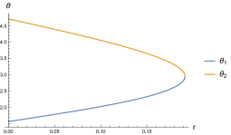
It was shown in Chaudhuri:2020xxb that for all the fixed points where the baryon symmetry in a sector is spontanously broken at nonzero temperatures, this phenomenon is accompanied by the Higgsing of half of the gauge bosons in the same sector. This leads the system to be in a persistent Brout-Englert-Higgs (BEH) phase at all nonzero temperatures.

A similar spontaneous breaking of a baryon symmetry at nonzero temperatures and a persistent BEH phase were also found at the corresponding fixed points of the dual CDB model. In this case, the relevant baryon symmetry in each sector is a $U(1)$ symmetry which can be obtained by replacing $\mathcal{T}_{i}$ by the $N_{ci}\times N_{ci}$ diagonal matrix defined below:

$$(\mathcal{T}_{i})_{\phi}\equiv\text{diag}\{e^{i\phi},1,\cdots,1\}.$$ (13)

with $\phi\in[0,2\pi)$.

An important result which was derived in Chaudhuri:2020xxb is that the above-mentioned baryon symmetries are not broken in a thermal state for the fixed points where the two sectors are decoupled. We will find this result to be consequential as one of these fixed points is the IR limit of the RG flows corresponding to the marginally relevant deformations discussed in section 3.

3 Phase transitions for marginally relevant deformations

In this section we will consider certain marginally relevant deformations of the points on the fixed circle in the RDB model by varying the quartic couplings between the scalars fields. In subsection 3.1 we will demonstrate the existence of such a marginally relevant deformation for each point on the fixed circle. Later in subsection 3.2 we will study the RG flows triggered by these deformations. We will show that in the IR limit these RG flows take the corresponding systems to a unique fixed point that lacks thermal order. Therefore, at low temperatures all these systems are in a disordered phase. On the other hand, in the UV limit some of these systems flow to the points on the fixed circle which exhibit thermal order. This means that at high temperatures these systems are in an ordered phase. Therefore, each of these systems must undergo an inverse symmetry breaking phase transition at some critical temperature. Above this critical temperature, the system remains persistently in a symmetry-broken phase. In subsection 3.3, we will provide an estimate of this critical temperature.

3.1 Deformations of the double trace quartic couplings

Let us now turn our attention to the deformations of the quartic couplings away from their values on the fixed circle. The deformations that are of interest to us involve only the double trace couplings ($f_{i}$ and $\zeta$). Since the beta functions of the single trace couplings ($\lambda_{i}$ and $h_{i}$) are independent of the double trace ones at the Veneziano limit, these couplings remain frozen at their fixed point values throughout the RG flows triggered by such deformations. Therefore, all such RG flows take place only in a subspace where $\lambda_{1}=\lambda_{2}=\lambda$ and $h_{1}=h_{2}=h$ with $\lambda$ and $h$ being the values given in (7) at leading order in perturbation theory. In this subspace the full planar beta functions of the double trace couplings have the following forms :

$$\begin{split}&\beta_{f_{p}}=F_{1}(f_{p},\sqrt{f_{m}^{2}+\zeta^{2}}),\ \beta_{f_{m}}=f_{m}\widetilde{F}_{2}(f_{p},\sqrt{f_{m}^{2}+\zeta^{2}}),\ \beta_{\zeta}=\zeta\widetilde{F}_{2}(f_{p},\sqrt{f_{m}^{2}+\zeta^{2}}),\end{split}$$ (14)

where $F_{1}$ and $\widetilde{F}_{2}$ are two functions of $f_{p}$ and $\sqrt{f_{m}^{2}+\zeta^{2}}$. Switching to the polar coordinates introduced in (10), the beta functions can be re-expressed as

$$\begin{split}&\beta_{f_{p}}=F_{1}(f_{p},R),\ \beta_{R}=F_{2}(f_{p},R),\ R\beta_{\theta}=0,\end{split}$$ (15)

where $F_{2}(f_{p},R)\equiv R\widetilde{F}_{2}(f_{p},R)$. The expressions of $F_{1}(f_{p},R)$ and $F_{2}(f_{p},R)$ at leading order are

$$\begin{split}&F_{1}(f_{p},R)=(8f_{p}+32h-6\lambda)f_{p}+8R^{2}+24h^{2}+\frac{9}{16}\lambda^{2}\ ,\\ &F_{2}(f_{p},R)=R(16f_{p}+32h-6\lambda)\ .\\ \end{split}$$ (16)

We can see that $\beta_{\theta}=0$ for all points in the space of the double trace couplings where $R\neq 0$. Moreover, the beta functions of $f_{p}$ and $R$ are independent of the angular coordinate $\theta$. Therefore, for a fixed point of these beta functions where $R\neq 0$, a shift in the value of $\theta$ spans the conformal manifold. Another important consequence of the vanishing of $\beta_{\theta}$ is that the projections of all RG flows on the $f_{m}$-$\zeta$ plane are radially directed. Furthermore, the fact that $\beta_{f_{p}}$ and $\beta_{R}$ are independent of $\theta$ ensures that such flows are identical for all values of $\theta$.

Now, suppose $f_{0p}$ and $R_{0}$ are the values of $f_{p}$ and $R$ for the points on the conformal manifold. The leading order expressions of $f_{0p}$ and $R_{0}$ are (see (7))

$$f_{0p}=\frac{\sqrt{6}}{8}\lambda,\ R_{0}=\Big{(}\frac{\sqrt{18\sqrt{6}-39}}{16}\Big{)}\lambda.$$ (17)

Consider the following small deformations of $f_{p}$ and $R$ away from their values on the fixed circle:

$$f_{p}=f_{0p}+\delta f_{p},\ R=R_{0}+\delta R.$$ (18)

The beta functions of these deformations in the values of $f_{p}$ and $R$ (at linear order) are

$$\begin{split}&\beta_{\delta f_{p}}=\frac{\partial F_{1}}{\partial f_{p}}(f_{0p},R_{0})\delta f_{p}+\frac{\partial F_{1}}{\partial R}(f_{0p},R_{0})\delta R,\\ &\beta_{\delta R}=\frac{\partial F_{2}}{\partial f_{p}}(f_{0p},R_{0})\delta f_{p}+\frac{\partial F_{2}}{\partial R}(f_{0p},R_{0})\delta R.\end{split}$$ (19)

The coefficient matrix multiplying the deformations in the above equations is

$$\mathcal{M}=\begin{pmatrix}\frac{\partial F_{1}}{\partial f_{p}}(f_{0p},R_{0})&\frac{\partial F_{1}}{\partial R}(f_{0p},R_{0})\\ \frac{\partial F_{2}}{\partial f_{p}}(f_{0p},R_{0})&\frac{\partial F_{2}}{\partial R}(f_{0p},R_{0})\end{pmatrix}=16R_{0}\begin{pmatrix}0&1\\ 1&0\end{pmatrix}.$$ (20)

The second equality in the above equation is obtained by substituting $F_{1}$, $F_{2}$ and the couplings $h$, $f_{0p}$ and $R_{0}$ by their leading order expressions. The eigenvalues of this matrix and the corresponding eigenvectors are as follows:

$$\begin{split}&v_{1}=-16R_{0},\ v_{2}=16R_{0},\\ &e_{1}=\begin{pmatrix}1\\ -1\end{pmatrix},\ e_{2}=\begin{pmatrix}1\\ 1\end{pmatrix}.\end{split}$$ (21)

Therefore, the deformations along $e_{1}$ and $e_{2}$ are marginally relevant and marginally irrelevant respectively. The existence of a marginally relevant deformation clearly demonstrates that all points on the conformal manifold are UV fixed points of certain RG flows. Next, let us study the features of these RG flows.

3.2 RG flows triggered by the marginally relevant deformations

To analyze the RG flows triggered by the marginally relevant deformations, we will rely on the 1-loop expressions of the beta functions. This approximation is justified near the UV fixed points on the conformal manifold as these fixed points are weakly coupled. However, the RG flows triggered by the marginally relevant deformations can take the system to a strongly coupled regime. We will show that this is not the case when we choose the marginally relevant deformation such that it has a radially inward component in the $f_{m}$-$\zeta$ plane, i.e., $\delta R<0$. Therefore, in this case one can trust the results based on the 1-loop beta functions. If the deformation is chosen to be in the opposite direction, i.e., $\delta R>0$, then the theory indeed flows to a strongly coupled regime. This can be verified by noticing that the RG flows obtained from the 1-loop beta functions lead to divergences of the couplings at finite energy scales.

With the above comments in mind, we choose the marginally relevant deformation to be

$$\delta f_{p}=-\delta R=\frac{R_{0}}{2}\widetilde{\epsilon}$$ (22)

at a reference energy scale $\Lambda$. We take $0<\widetilde{\epsilon}<1$. The RG flow generated by the 1-loop beta functions leads to the following values of the couplings at a scale $\mu$:

$$\begin{split}&f_{p}=f_{0p}+\frac{R_{0}}{2}\Bigg{[}\frac{(1-k)\Big{(}1-\tanh(8R_{0}t)\Big{)}}{1+k\tanh(8R_{0}t)}\Bigg{]}\ ,\ R=\frac{R_{0}}{2}\Bigg{[}\frac{(1+k)\Big{(}1+\tanh(8R_{0}t)\Big{)}}{1+k\tanh(8R_{0}t)}\Bigg{]}\ ,\\ \end{split}$$ (23)

where $t\equiv\ln(\mu/\Lambda)$ and $k\equiv 1-\widetilde{\epsilon}$. In figure 3, a graphical plot of this RG flow is given for $\lambda=0.001,\ \widetilde{\epsilon}=0.1$.

Figure 3: RG flow for $\lambda=0.001,\ \widetilde{\epsilon}=0.1$: In the UV limit ($t\rightarrow\infty$) the couplings flow to a point on the fixed circle. In the IR limit ($t\rightarrow-\infty$) they flow to a fixed point where the two sectors are decoupled.

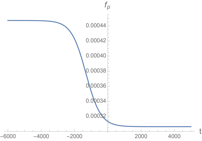
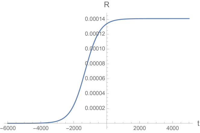
Note that the theory remains weakly coupled throughout the RG flow. In the deep UV, it flows to a point on the fixed circle as expected. In the deep IR, it flows to a fixed point where the two sectors are decoupled and $f_{1}=f_{2}={2\sqrt{6}+\sqrt{18\sqrt{6}-39}\over 16}\lambda$. Due to the rotational symmetry in the $f_{m}$-$\zeta$ plane, this behavior of the RG flow is identical for marginally relevant deformations of all points on the fixed circle. In particular, when $r<r_{\text{max}}$, it holds for the deformations of the fixed points demonstrating thermal order in the second sector. The RG flows triggered by these deformations lead to the IR fixed point where the two sectors are decoupled. As we have mentioned earlier, the baryon symmetries in both the sectors are unbroken at any nonzero temperature for this IR fixed point. Therefore, for the systems that flow from the UV fixed points with thermal order to this IR fixed point without thermal order, there must be a transition from a disordered phase to an ordered phase as the temperature is increased. We will now determine the critical temperatures at which this phase transition takes place in these systems.

3.3 Estimates of the critical temperatures

To determine the critical temperatures, we will consider the thermal effective potential of the scalar fields. At leading order in perturbation theory, this potential has both quadratic and quartic terms. The quartic terms are as follows:

$$V_{\text{quartic}}=16\pi^{2}\Bigg{[}\sum_{i=1}^{2}\frac{h_{i}}{N_{ci}}\text{Tr}[(\Phi_{i}^{T}\Phi_{i})^{2}]+\sum_{i=1}^{2}\frac{f_{i}}{N_{ci}^{2}}\Big{(}\text{Tr}[\Phi_{i}^{T}\Phi_{i}]\Big{)}^{2}+\frac{2\zeta}{N_{c1}N_{c2}}\text{Tr}[\Phi_{1}^{T}\Phi_{1}]\text{Tr}[\Phi_{2}^{T}\Phi_{2}]\Bigg{]}.$$ (24)

In appendix A we have shown that these quartic terms are positive-definite throughout the RG flows that we have discussed in the previous subsection.

The quadratic terms in the thermal effective potential are generated due to integration over the nonzero Matsubara modes of the different fields in the theory. These terms have the following structure

$$V_{\text{quadratic}}=\frac{1}{2}\sum_{i=1}^{2}m_{\text{th},i}^{2}\text{Tr}[\Phi_{i}^{T}\Phi_{i}]$$ (25)

where $m_{\text{th},1}^{2}$ and $m_{\text{th},2}^{2}$ are the thermal masses (squared) of the scalar fields $\Phi_{1}$ and $\Phi_{2}$ respectively. The contributions of 1-loop diagrams to such thermal masses (squared) were computed for a general 4-dimensional gauge theory in Weinberg:1974hy . Using these general results, the 1-loop expressions of $m_{\text{th},1}^{2}$ and $m_{\text{th},2}^{2}$ were derived in Chaudhuri:2020xxb . These expressions reduce to the following forms at the planar limit:

$$\begin{split}&m_{\text{th},1}^{2}=\frac{16\pi^{2}T^{2}}{3}\Bigg{[}2h_{1}+f_{1}+r\zeta+\frac{3}{8}\lambda_{1}\Bigg{]},\\ &m_{\text{th},2}^{2}=\frac{16\pi^{2}T^{2}}{3}\Bigg{[}2h_{2}+f_{2}+\frac{\zeta}{r}+\frac{3}{8}\lambda_{2}\Bigg{]},\\ \end{split}$$ (26)

where $T$ is the temperature. These thermal masses (squared) quantify the behavior of the effective potential of the scalar fields in the neighborhood of the point $\Phi_{1}=\Phi_{2}=0$, viz., the origin of the field space. Their signs determine the fates of the baryon symmetries at any given temperature. If either $m_{\text{th},1}^{2}$ or $m_{\text{th},2}^{2}$ is negative then the minimum of the effective potential cannot be at the origin of the field space. In fact, the positivity of the tree-level quartic terms in the potential ensures the existence of a minimum of the potential away from the origin. This would imply the spontaneous breaking of at least one of the baryon symmetries. In particular, when $m_{\text{th},i}^{2}<0$, the baryon symmetry in the $i^{\text{th}}$ sector would be spontaneously broken Chaudhuri:2020xxb .

To track the effective potential at different temperatures we will set the renormalization scale $\mu=T$. Let us explain this choice of the renormalization scale. Our aim is to check perturbatively whether the thermal effective potential of the scalar fields has a minimum away from the origin. When both the thermal masses (squared) are positive, the minimum of the potential is at the origin. In this case, as long as we are sufficiently away from the critical temperature, we will have $m_{\text{th},1}^{2},m_{\text{th},2}^{2}\sim\frac{16\pi^{2}}{3}\lambda T^{2}$. At higher orders in the perturbative expansion of the potential near the origin, there are terms which contain the logarithm of the ratio of $m_{\text{th},i}^{2}$ and $\mu^{2}$. The lowest order term of this kind is the Coleman-Weinberg term Coleman:1973jx ; Lee:1974fj ; Gould:2021oba . By setting $\mu=T$ we ensure that such logarithmic terms are suppressed by at least a factor of $\lambda\ln\lambda\ll 1$ compared to the leading order terms that we are retaining. A similar argument can be given when either of the thermal masses (squared) is negative and the minimum of the potential is away from the origin. In this case, again as long as we are sufficiently away from the critical point, we will have $|m_{\text{th},i}^{2}|\sim\frac{16\pi^{2}}{3}\lambda T^{2}$ irrespective of the sign of $m_{\text{th},i}^{2}$. Comparing this behavior of the thermal masses (squared) with the quartic terms given in (24), one can check that if there is symmetry-breaking in the $i^{\text{th}}$ sector, then the value of $\Phi_{i}$ (appropriately normalized by $N_{ci}$) at the minimum would be of the same order as the temperature scale $T$. To be more precise, if $(\Phi_{i})_{0}$ is the value of $\Phi_{i}$ at the minimum, then $\frac{\sqrt{\text{Tr}[(\Phi_{i})_{0}^{T}(\Phi_{i})_{0}]}}{N_{ci}}\sim T$. We want the perturbative expansion of the potential to be valid at this scale. At higher orders in this expansion, there are terms which contain the logarithm of the ratio of $\lambda$ times the square of this scale and $\mu^{2}$. By taking $\mu=T$, we again ensure that such logarithmic corrections are small. So we can rely on the perturbative analysis sufficiently away from the critical temperature on both sides of this temperature. To come up with an estimate of the critical temperature, we will interpolate the thermal masses (squared) in the intermediate interval with the expressions given in (26) and search for the point at which one of the thermal masses (squared) vanishes.

One may be able to improve the above-mentioned perturbative analysis by choosing $\mu$ to be some $O(1)$ numerical coefficient times $T$. Such a numerical factor can be absorbed in the reference energy scale $\Lambda$ by rescaling it appropriately while doing thermal perturbation theory. Due to the ambiguity in the value of this numerical factor, there would be theoretical uncertainties in the critical temperatures of the phase transitions that we will study. Henceforth, we will ignore this subtlety as our aim is to find the qualitative nature of the phases in different temperature regimes and to determine the critical temperatures for the phase transitions in terms of the unspecified reference energy scale $\Lambda$.

Having provided the rationale for choosing $\mu=T$ in the effective potential, let us now look at the behavior of the thermal masses at different temperature scales. For this it is convenient to define the dimensionless quantity

$$\widetilde{m}_{\text{th},i}^{2}\equiv\frac{3}{16\pi^{2}T^{2}}m_{\text{th},i}^{2}.$$ (27)

Substituting the values of the the different couplings along the RG flow triggered by the marginally relevant deformation, we get

$$\begin{split}\widetilde{m}_{\text{th},1}^{2}=&\frac{R_{0}}{2}(1+k)\Big{(}r\cos\theta+\sin\theta-1\Big{)}C(t)+\Big{(}\frac{3}{4}\lambda+R_{0}\Big{)},\\ \widetilde{m}_{\text{th},2}^{2}=&\frac{R_{0}}{2}(1+k)\Big{(}\frac{\cos\theta}{r}-\sin\theta-1\Big{)}C(t)+\Big{(}\frac{3}{4}\lambda+R_{0}\Big{)},\\ \end{split}$$ (28)

where $\theta$ is the angular location of the UV fixed point on the conformal manifold and $C(t)$ is the following function of $t\equiv\ln(\frac{T}{\Lambda})$:

$$C(t)\equiv\frac{1+\tanh(8R_{0}t)}{1+k\tanh(8R_{0}t)}.$$ (29)

Note that the parameter $k=1-\widetilde{\epsilon}$ controls the behavior of the thermal masses at different temperatures. As $\widetilde{\epsilon}\rightarrow 0$, $C(t)\rightarrow 1$ and the rescaled thermal masses (squared), $\widetilde{m}_{\text{th},1}^{2}$ and $\widetilde{m}_{\text{th},2}^{2}$, stop changing with the temperature. In this limit, they just reduce to the rescaled thermal masses (squared) of the points on the conformal manifold which were analyzed in Chaudhuri:2020xxb .

To study the variations of the thermal masses (squared) with the temperature concretely, we choose the UV fixed point to be the point where $\theta=\pi$, or equivalently, $f_{m}=0,\ \zeta=-R_{0}$. As can be verified from (11), this fixed point has thermal order in the second sector only when $r<r_{0}\approx 0.188$. So to stay in this regime, we choose $r=0.1$. To keep the values of the couplings and the deformations small we choose $\lambda=0.001$ and $\widetilde{\epsilon}=0.1$ as before. For this set of parameters, the plots of the rescaled thermal masses (squared) at different temperature scales are given in figure 4.

Figure 4: Plots of the rescaled thermal masses (squared) against $t=\ln(T/\Lambda)$ for $r=0.1$, $\theta=\pi$, $\lambda=0.001$, $\widetilde{\epsilon}=0.1$: In the low temperature regime, both $\widetilde{m}_{\text{th},1}^{2}$ and $\widetilde{m}_{\text{th},2}^{2}$ saturate at positive values. This indicates that the baryon symmetries in both the sectors are unbroken in this regime. In the high temperature limit, $\widetilde{m}_{\text{th},1}^{2}$ saturates at a positive value, while $\widetilde{m}_{\text{th},2}^{2}$ saturates at a negative value. This means that the baryon symmetry in the second sector remains persistently broken above a critical temperature. This critical temperature ($T_{c}$) is given by $t_{c}\equiv\ln(T_{c}/\Lambda)\approx-1172.1$.

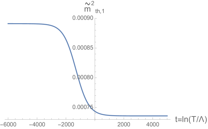
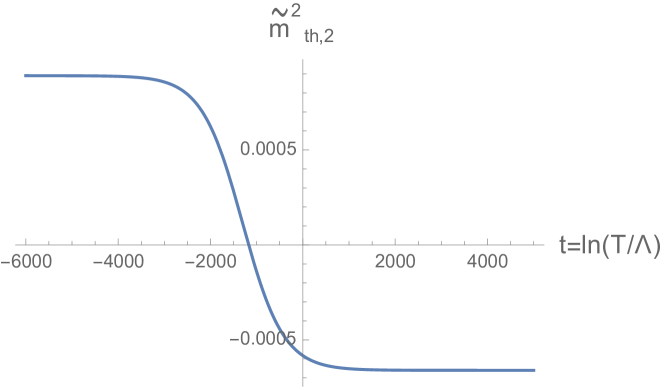
As one can see form these plots, both $\widetilde{m}_{\text{th},1}^{2}$ and $\widetilde{m}_{\text{th},2}^{2}$ decrease monotonically with increase in the temperature. However, $\widetilde{m}_{\text{th},1}^{2}$ remains positive at all temperatures indicating the absence of thermal order in the first sector. On the other hand, $\widetilde{m}_{\text{th},2}^{2}$ starts off from a positive value at low temperatures, but eventually becomes negative at high temperatures indicating a transition to an ordered phase. The critical temperature at which this transition happens is where $\widetilde{m}_{\text{th},2}^{2}=0$. This behavior is similar for all the systems where the UV fixed point exhibits thermal order in the second sector. One can obtain a general expression of the critical temperature ($T_{c}\equiv\Lambda e^{t_{c}}$) for all these systems by solving the equation $\widetilde{m}_{\text{th},2}^{2}=0$. We provide this expression below:

$$t_{c}=\frac{1}{8R_{0}}\tanh^{-1}(\rho),$$ (30)

where

$$\rho\equiv\frac{-(1+k)\frac{R_{0}}{2r}\Big{(}-\cos\theta+r(1+\sin\theta)\Big{)}+(\frac{3\lambda}{4}+R_{0})}{(1+k)\frac{R_{0}}{2r}\Big{(}-\cos\theta+r(1+\sin\theta)\Big{)}-k(\frac{3\lambda}{4}+R_{0})}.$$ (31)

From the above expression, we can see that $t_{c}$ has a real value only when $\rho\in(-1,1)$. This puts a restriction on the UV fixed points for which there can be a phase transition. The allowed fixed points are precisely the ones where $\theta\in(\theta_{1},\theta_{2})$ with $\theta_{1}$ and $\theta_{2}$ being the values given in (11). To study the variation of $t_{c}$ in this domain, we choose $r=0.1$, $\lambda=0.001$, $\widetilde{\epsilon}=0.1$ and plot the values of $t_{c}$ for different values of $\theta$ in figure 5.

Figure 5: Plot of $t_{c}$ against $\theta$ for $r=0.1,\lambda=0.001,\ \widetilde{\epsilon}=0.1$: The critical temperature increases sharply near the edges of the interval $(\theta_{1},\theta_{2})$, i.e., $t_{c}\rightarrow\infty$ as $\theta\rightarrow\theta_{1}$ or $\theta\rightarrow\theta_{2}$.

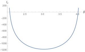
As one can see, $t_{c}$ increases rapidly as one approaches the edges of the interval $(\theta_{1},\theta_{2})$. As $\theta\rightarrow\theta_{1}$ or $\theta\rightarrow\theta_{2}$, $t_{c}\rightarrow\infty$ thereby indicating the absence of the phase transition at the end points. For each point in the interval $\theta\in(\theta_{1},\theta_{2})$, there is a finite temperature at which the system goes to an ordered phase characterized by the spontaneous breaking of the baryon symmetry and Higgsing of half of the gauge bosons in the second sector. In the Veneziano limit, the system remains in this phase at all higher temperatures.

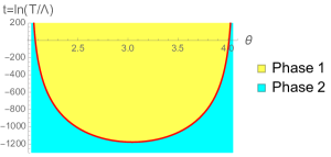
The line of critical points shown in figure 5 separates the following two phases:

• Phase 1: The high temperature phase where the baryon symmetry in the first sector remains unbroken while the baryon symmetry in the second sector is spontaneously broken.

• Phase 2: The low temperature phase where the baryon symmetries in both the sectors are unbroken.

In figure 6, we show the phase diagram of the systems with $r=0.1$, $\lambda=0.001$, $\widetilde{\epsilon}=0.1$. The phase diagrams for other values of $r$ in the domain $r<r_{\text{max}}$ would be similar to that shown in this figure.

Figure 6: Phase diagram of the systems with $r=0.1$, $\lambda=0.001$, $\widetilde{\epsilon}=0.1$: In Phase 1, the baryon symmetry in the first sector is unbroken while the baryon symmetry in the second sector is spontaneously broken. In Phase 2, the baryon symmetries in both the sectors are unbroken. The red line in this diagram is the line of critical points separating the two phases. It is the same as the curve given in figure 5.

Let us end this section with a remark on the zero temperature phase of the systems that we have been considering. At $T=0$, the thermal masses (squared) vanish and it is no longer possible to set the renormalization scale $\mu$ to $T$. In this case, one may wonder whether the Coleman-Weinberg terms can lead to a symmetry-broken phase. Such a symmetry-broken phase was indeed found in Coleman:1973jx for massless scalar QED at zero temperature. As shown in Coleman:1973jx , the quartic coupling in that model is of the same order as the fourth power of the gauge coupling at certain renormalization scales. This leads to the Coleman-Weinberg term becoming comparable to the quartic term slightly away from the origin which, in turn, allows for a perturbatively reliable minimum in this domain. In our case, however, the quartic couplings remain $O(\lambda)$ throughout the RG flow with $\lambda$ being related to the gauge couplings $g_{i}$ by $\lambda=\frac{N_{ci}g_{i}^{2}}{16\pi^{2}}$. The suppression of the Coleman-Weinberg terms compared to the quartic terms in this case is analogous to the same in massless $\phi^{4}$ theory where one does not get a perturbatively reliable minimum away from the origin at zero temperature Coleman:1973jx . Therefore, in the systems that we are considering, we expect the baryon symmetries in both the sectors to remain unbroken at zero temperature. We would like to establish this more rigorously in the future.

4 Adding masses to the scalar fields

In the previous section we studied marginally relevant deformations of the points on the fixed circle in the RDB model obtained by varying the double trace quartic couplings between the scalar fields. In this section we will consider relevant deformations of the same fixed points obtained by adding masses to the scalar fields. For such deformations, the Lagrangian has the following terms in addition to those given in (2):

$$\mathcal{L}_{\text{mass}}=-\frac{1}{2}\sum_{i=1}^{2}m_{i}^{2}\text{Tr}[\Phi_{i}^{T}\Phi_{i}],$$ (32)

where $m_{1}^{2}$ and $m_{2}^{2}$ are the renormalized masses (squared) of the scalar fields in the two sectors. The 1-loop planar contributions to their RG flows (in the $\overline{\text{MS}}$ scheme) are derived in appendix B. These contributions are as follows:

$$\begin{split}&\mu\frac{dm_{1}^{2}}{d\mu}=\Big{(}16h_{1}+8f_{1}-3\lambda_{1}\Big{)}m_{1}^{2}+8r\zeta m_{2}^{2},\\ &\mu\frac{dm_{2}^{2}}{d\mu}=\Big{(}16h_{2}+8f_{2}-3\lambda_{2}\Big{)}m_{2}^{2}+\frac{8\zeta}{r}m_{1}^{2}.\end{split}$$ (33)

Since we are working in a mass-independent renormalization scheme for the RG flows of the quartic couplings, we can freeze these couplings at their fixed point values and study the flows of the masses. Substituting the couplings by their leading order values on the fixed circle as given in (7) and switching to the polar coordinates in the $f_{m}$-$\zeta$ plane (see (10)), we get

$$\begin{split}&\mu\frac{dm_{1}^{2}}{d\mu}=8R_{0}\Big{(}\sin\theta\ m_{1}^{2}+r\cos\theta\ m_{2}^{2}\Big{)},\\ &\mu\frac{dm_{2}^{2}}{d\mu}=8R_{0}\Big{(}\frac{\cos\theta}{r}\ m_{1}^{2}-\sin\theta\ m_{2}^{2}\Big{)},\end{split}$$ (34)

where $R_{0}$ is the radius of the fixed circle whose value at leading order in $\lambda$ is given by

$$R_{0}=\Big{(}\frac{\sqrt{18\sqrt{6}-39}}{16}\Big{)}\lambda.$$ (35)

Solving the above equations, we get

$$\begin{split}&m_{1}^{2}=\frac{1}{2}(1-\sin\theta)M_{1}^{2}\ e^{-8R_{0}t}+\frac{1}{2}(1+\sin\theta)M_{2}^{2}\ e^{8R_{0}t},\\ &m_{2}^{2}=\frac{1}{2r}\Big{(}-M_{1}^{2}\ e^{-8R_{0}t}+M_{2}^{2}\ e^{8R_{0}t}\Big{)}\cos\theta,\end{split}$$ (36)

where $t\equiv\ln(\mu/\Lambda)$ with $\Lambda$ being a reference energy scale. $M_{1}^{2}$ and $M_{2}^{2}$ are integration constants having the dimension of mass². When both of them are nonzero, they determine the asymptotic behavior of the renormalized masses (squared) in the IR and UV regimes respectively.

At any nonzero temperature $T$ there are additional contributions to the effective masses (squared) of the scalar fields from the the thermal masses (squared) which were discussed in the previous section. For the massive theories that we are considering presently, the expressions of the 1-loop thermal masses (squared) given in (26) are approximately valid when $T^{2}\gg|m_{i}^{2}|$. These expressions are given below:

$$\begin{split}&m_{\text{th},1}^{2}=\frac{16\pi^{2}T^{2}}{3}\Bigg{[}2h_{1}+f_{1}+r\zeta+\frac{3}{8}\lambda_{1}\Bigg{]},\\ &m_{\text{th},2}^{2}=\frac{16\pi^{2}T^{2}}{3}\Bigg{[}2h_{2}+f_{2}+\frac{\zeta}{r}+\frac{3}{8}\lambda_{2}\Bigg{]}.\\ \end{split}$$ (37)

For the points on the fixed circle, these expressions reduce to

$$\begin{split}m_{\text{th},1}^{2}=&\frac{16\pi^{2}T^{2}}{3}\Bigg{[}R_{0}\Big{(}r\cos\theta+\sin\theta\Big{)}+\frac{3}{4}\lambda\Bigg{]},\\ m_{\text{th},2}^{2}=&\frac{16\pi^{2}T^{2}}{3}\Bigg{[}R_{0}\Big{(}\frac{\cos\theta}{r}-\sin\theta\Big{)}+\frac{3}{4}\lambda\Bigg{]}.\\ \end{split}$$ (38)

The overall effective masses (squared) of the scalar fields at the temperature $T$ are

$$\begin{split}&m_{\text{eff},1}^{2}=(m_{1}^{2}+m_{\text{th},1}^{2})|_{\mu=T},\ m_{\text{eff},2}^{2}=(m_{2}^{2}+m_{\text{th},2}^{2})|_{\mu=T}.\end{split}$$ (39)

These effective masses (squared) determine the behavior of the effective potential of the scalar fields in the neighborhood of the point $\Phi_{1}=\Phi_{2}=0$. A negative value of $m_{\text{eff},i}^{2}$ indicates that the baryon symmetry in the $i^{\text{th}}$ sector is spontaneously broken.

Here, as in the previous section, we have set $\mu=T$ to avoid large logarithms from appearing in the thermal perturbative expansion of the effective potential of the scalar fields. However, now one must be careful as the validity of this choice of the renormalization scale rests on the magnitudes of effective masses (squared) being $O(\frac{16\pi^{2}}{3}\lambda T^{2})$. At sufficiently low temperatures, the contributions of the renormalized masses (squared) will drive the effective masses (squared) out of this regime. So, unlike the previous section, here we cannot study the phase of the system down to arbitrarily low temperatures. However, we will show that in some cases, the renormalized masses can induce a phase transition at scales where the perturbative analysis is reliable, i.e., near the critical temperatures corresponding to these phase transitions, the effective masses (squared) remain $O(\frac{16\pi^{2}}{3}\lambda T^{2})$. In the rest of this section, we will use the term ‘low temperatures’ to mean temperatures slightly below such critical temperatures where the perturbative analysis is valid. We hope the reader will not be misled by this laxity.

The above-mentioned phase transitions and the corresponding critical temperatures depend on the magnitudes and the signs of two mass² scales $M_{1}^{2}$ and $M_{2}^{2}$ which were introduced in (36). To study these phase transitions let us define the following two dimensionless quantities which are obtained via dividing $M_{1}^{2}$ and $M_{2}^{2}$ by $\frac{32\pi^{2}}{3}\Lambda^{2}$:

$$c_{1}\equiv\frac{3}{32\pi^{2}}\frac{M_{1}^{2}}{\Lambda^{2}},\ c_{2}\equiv\frac{3}{32\pi^{2}}\frac{M_{2}^{2}}{\Lambda^{2}}.$$ (41)

It is also convenient to switch to the following dimensionless quantities obtained via dividing the effective masses (squared) by $\frac{16\pi^{2}}{3}T^{2}$ :

$$\widetilde{m}_{\text{eff},1}^{2}\equiv\frac{3}{16\pi^{2}}\frac{m_{\text{eff},1}^{2}}{T^{2}},\ \widetilde{m}_{\text{eff},2}^{2}\equiv\frac{3}{16\pi^{2}}\frac{m_{\text{eff},2}^{2}}{T^{2}}.$$ (42)

In the regime where $m_{i}^{2}|_{\mu=T}\ll T^{2}$ and the expressions of the thermal masses (squared) given in (38) are reliable, the rescaled effective masses (squared) defined above have the following values:

$$\begin{split}&\widetilde{m}_{\text{eff},1}^{2}=(1-\sin\theta)c_{1}\ e^{-(2+8R_{0})t}+(1+\sin\theta)c_{2}\ e^{-(2-8R_{0})t}+R_{0}\Big{(}r\cos\theta+\sin\theta\Big{)}+\frac{3}{4}\lambda,\\ &\widetilde{m}_{\text{eff},2}^{2}=\frac{1}{r}\Big{(}-c_{1}\ e^{-(2+8R_{0})t}+c_{2}\ e^{-(2-8R_{0})t}\Big{)}\cos\theta+R_{0}\Big{(}\frac{\cos\theta}{r}-\sin\theta\Big{)}+\frac{3}{4}\lambda.\end{split}$$ (43)

In the high temperature limit (i.e., large $t$), the rescaled effective masses (squared) are dominated by the contributions of the thermal masses (squared) and we have

$$\begin{split}&\widetilde{m}_{\text{eff},1}^{2}\xrightarrow{t\rightarrow\infty}R_{0}\Big{(}r\cos\theta+\sin\theta\Big{)}+\frac{3}{4}\lambda,\\ &\widetilde{m}_{\text{eff},2}^{2}\xrightarrow{t\rightarrow\infty}R_{0}\Big{(}\frac{\cos\theta}{r}-\sin\theta\Big{)}+\frac{3}{4}\lambda.\end{split}$$ (44)

These high temperature behaviors of the effective masses (squared) are exactly as they would be for the UV CFTs. Therefore, for the systems where $r<r_{\text{max}}=\sqrt{\frac{6\sqrt{6}-13}{61-6\sqrt{6}}}$ and $\theta\in(\theta_{1},\theta_{2})$ with $\theta_{1}$ and $\theta_{2}$ being the values given in (11), the baryon symmetry in the first sector remains unbroken in the high temperature regime, whereas the baryon symmetry in the second sector is persistently broken in the same regime. In the rest of this section we will restrict our attention to these systems which exhibit thermal order in the second sector at the high temperature limit. As the temperature is lowered in these systems, i.e., as $t$ decreases, the contributions of the renormalized masses (squared) start becoming comparable to the thermal masses (squared). This is what allows for phase transitions in the system. From the expressions given in (43) one can see that the signs of $c_{1}$ and $c_{2}$ (or equivalently, the signs of the mass² scales $M_{1}^{2}$ and $M_{2}^{2}$) play the key role in determining these phase transitions. We will study these phase transitions in the following 2 cases:

• Case 1: $M_{1}^{2}\neq 0,M_{2}^{2}=0$,

• Case 2: $M_{1}^{2}=0,M_{2}^{2}\neq 0$.

We will see that for each of these cases, there are distinct patterns of phase transitions depending on the signs of the nonzero $M_{i}^{2}$. We will discuss the low temperature phases for the different signs of the nonzero $M_{i}^{2}$ in each case as separate subcases. Later, in subsection 4.3 we will summarize these results and comment on the possible phase transitions when both $M_{1}^{2}$ and $M_{2}^{2}$ are nonzero.

4.1 Case 1: $M_{1}^{2}\neq 0,M_{2}^{2}=0$

In this case the expressions of the rescaled effective masses (squared) reduce to the following forms:

$$\begin{split}&\widetilde{m}_{\text{eff},1}^{2}=(1-\sin\theta)c_{1}\ e^{-(2+8R_{0})t}+R_{0}\Big{(}r\cos\theta+\sin\theta\Big{)}+\frac{3}{4}\lambda,\\ &\widetilde{m}_{\text{eff},2}^{2}=-\frac{1}{r}\cos\theta\ c_{1}\ e^{-(2+8R_{0})t}+R_{0}\Big{(}\frac{\cos\theta}{r}-\sin\theta\Big{)}+\frac{3}{4}\lambda.\end{split}$$ (45)

We remind the reader that we are restricting our attention to the systems which exhibit thermal order in the second sector at high temperatures, i.e., the systems where $r<r_{\text{max}}$ and $\theta\in(\theta_{1},\theta_{2})$. As we have already mentioned in section 2, $\cos\theta$ is always negative for such systems. Moreover, the quantity $(1-\sin\theta)$ is positive for all values of $\theta$ in this domain. Therefore, from the expressions given in (45) we can see that in the low temperature regime where the renormalized masses (squared) dominate over the thermal masses (squared), both the effective masses (squared) have the same sign. This sign depends on whether $c_{1}$ (or equivalently, $M_{1}^{2}$) is positive or negative.

4.1.1 Subcase 1: $M_{1}^{2}>0$

When $M_{1}^{2}>0$, both the effective masses (squared) are positive in the low temperature regime. This indicates that the baryon symmetries in both the sectors are unbroken in this regime. Therefore, there should be a phase transition at some critical temperature where the baryon symmetry in the second sector is spontaneously broken.

At the critical temperature ($T_{c}$) corresponding to this phase transition $m_{\text{eff},2}^{2}$ vanishes, i.e., the renormalized mass (squared) $m_{2}^{2}|_{\mu=T_{c}}$ exactly cancels the thermal mass (squared) $m_{\text{th},2}^{2}$ . Therefore, we have

$$|m_{2}^{2}|_{\mu=T_{c}}|\sim\frac{16\pi^{2}}{3}\lambda T_{c}^{2}\ll T_{c}^{2}.$$ (46)

Moreover, note that the two renormalized masses (squared) are related as follows

$$m_{1}^{2}|_{\mu=T_{c}}=\alpha m_{2}^{2}|_{\mu=T_{c}}$$ (47)

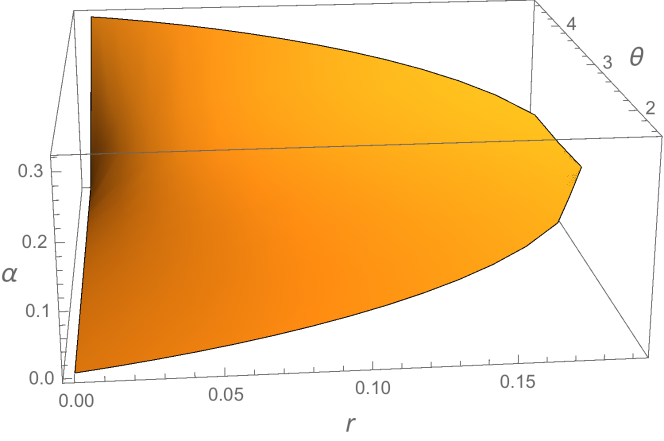
where $\alpha\equiv-\frac{r(1-\sin\theta)}{\cos\theta}$. Since we are considering systems where $r\in(0,r_{\text{max}})$ and $\theta\in(\theta_{1},\theta_{2})$ with $\theta_{1}$ and $\theta_{2}$ satisfying $\frac{\pi}{2}<\theta_{1}<\theta_{2}<\frac{3\pi}{2}$, both the numerator and denominator in $\alpha$ are nonzero. In fact, the denominator can become small only when $\theta$ is close to $\pi/2$ or $3\pi/2$. Such values of $\theta$ can lie in the range $(\theta_{1},\theta_{2})$ only when $r$ is close to zero. Therefore, in this case the factor of $r$ in the numerator of the expression of $\alpha$ ensures that $\alpha$ remains small despite the denominator having a small value. In figure 7 we show the values of $\alpha$ for all values $(r,\theta)$ satisfying $r<r_{\text{max}}$ and $\theta_{1}<\theta<\theta_{2}$. We can see that $\alpha<1$ at all points in this domain.

Figure 7: Plot of $\alpha=-\frac{r(1-\sin\theta)}{\cos\theta}$ against $r$ and $\theta$ in the domain $r<r_{\text{max}}$ and $\theta\in(\theta_{1},\theta_{2})$.

Thus, from (46) and (47) we can conclude that

$$|m_{1}^{2}|_{\mu=T_{c}}|\lesssim\frac{16\pi^{2}}{3}\lambda T_{c}^{2}\ll T_{c}^{2}$$ (48)

for all these systems. Note that $|m_{1,2}^{2}|_{\mu=T_{c}}|\ll T_{c}^{2}$ means that the expressions of the thermal masses (squared) given in (38) are reliable at the critical temperature. Moreover, the fact that $|m_{1}^{2}|_{\mu=T_{c}}|\lesssim\frac{16\pi^{2}}{3}\lambda T_{c}^{2}$ ensures that at the critical temperature $|m_{\text{eff},1}^{2}|\sim\frac{16\pi^{2}}{3}\lambda T_{c}^{2}$. This means that the perturbation theory with $\mu=T$ can be trusted at temperatures near $T_{c}$. Hence, one can study the phase transition using this renormalization scale.

To study this phase transition with a concrete example, we plot the rescaled effective masses (squared) against $t\equiv\ln(T/\Lambda)$ for the case where $r=0.1,\ \theta=\pi$, $\lambda=0.001$, $c_{1}=0.1$ and $c_{2}=0$ in figure 8. One can check that the choice of $r$ and $\theta$ is such that the UV fixed point exhibits thermal order in the second sector.

Figure 8: Plots of the rescaled effective masses (squared) against $t=\ln(T/\Lambda)$ for $r=0.1$, $\theta=\pi$, $\lambda=0.001$, $c_{1}=0.1$, $c_{2}=0$: Both $\widetilde{m}_{\text{eff},1}^{2}$ and $\widetilde{m}_{\text{eff},2}^{2}$ grow as the temperature decreases. In the high temperature limit, $\widetilde{m}_{\text{eff},1}^{2}$ saturates at a positive value while $\widetilde{m}_{\text{eff},2}^{2}$ saturates at a negative value. This indicates a phase transition at an intermediate temperature where the baryon symmetry in the second sector is broken. The critical temperature ($T_{c}$) corresponding to this phase transition is given by $t_{c}\equiv\ln(T_{c}/\Lambda)\approx 3.659$.

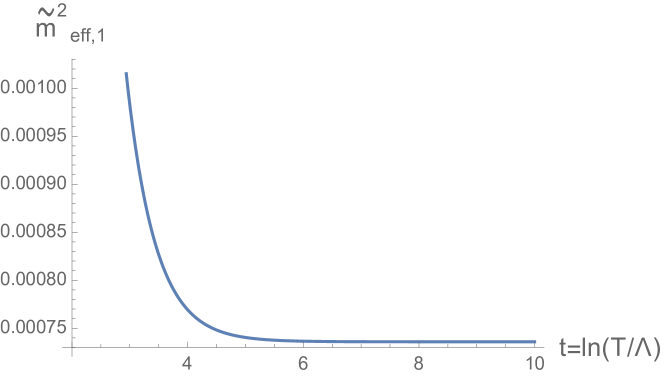
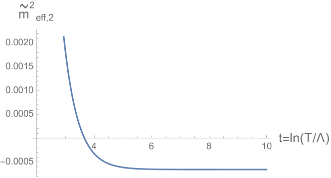
Note that $\widetilde{m}_{\text{eff},1}^{2}$ remains positive for all values of $t$. It grows as one goes to lower temperatures. At high temperatures, it saturates at a positive value. This means that the baryon symmetry in the first sector remains unbroken at all temperatures where the perturbative analysis is reliable. On the other hand, $\widetilde{m}_{\text{eff},2}^{2}$ also grows as the temperature is lowered, but at high temperatures it saturates at a negative value. This means that the baryon symmetry in the second sector is spontaneously broken at a critical temperature and then it remains broken at all higher temperatures.

In order to determine this critical temperature, we can solve for the value of $t$ at which $\widetilde{m}_{\text{eff},2}^{2}$ vanishes. Setting $\widetilde{m}_{\text{eff},2}^{2}=0$ at $t=t_{c}=\ln(T_{c}/\Lambda)$, we get

$$\begin{split}&t_{c}=-\frac{1}{2+8R_{0}}\ln\Bigg{[}\frac{r}{c_{1}\cos\theta}\Bigg{\{}R_{0}\Big{(}\frac{\cos\theta}{r}-\sin\theta\Big{)}+\frac{3}{4}\lambda\Bigg{\}}\Bigg{]}.\end{split}$$ (49)

In figure 9, we provide the plot of $t_{c}$ corresponding to different values of $\theta\in(\theta_{1},\theta_{2})$ for $\ r=0.1,\ \lambda=0.001,\ c_{1}=0.1,\ c_{2}=0$.

Figure 9: Plot of $t_{c}$ against $\theta$ for $r=0.1,\ \lambda=0.001,\ c_{1}=0.1,\ c_{2}=0$: The critical temperature increases sharply near the edges of the interval $(\theta_{1},\theta_{2})$,i.e., $t_{c}\rightarrow\infty$ as $\theta\rightarrow\theta_{1,2}$.

Just like what we saw for the critical temperatures corresponding to the phase transitions discussed in section 3, the critical temperature in this case increases sharply as one approaches the edges of the domain $(\theta_{1},\theta_{2})$, and $t_{c}\rightarrow\infty$ as $\theta\rightarrow\theta_{1}$ or $\theta\rightarrow\theta_{2}$. This means that at these edges, the system no longer undergoes the aforementioned phase transition and the baryon symmetries in both the sectors remain unbroken at all temperatures where the perturbative analysis can be trusted.

4.1.2 Subcase 2: $M_{1}^{2}<0$

When $M_{1}^{2}<0$, both the effective masses (squared) are negative in the low temperature regime. This means that the baryon symmetries in both the sectors are spontaneously broken in this regime. On the other hand, in the high temperature regime, the baryon symmetry in the first sector is unbroken while the baryon symmetry in the second sector is spontaneously broken. Therefore, we expect a phase transition at some critical temperature where the baryon symmetry in the first sector is restored.

At this critical temperature, the effective mass (squared) $m_{\text{eff},1}^{2}$ should vanish, i.e., $m_{1}^{2}|_{\mu=T_{c}}$ should cancel the contribution of the $m_{\text{th},1}^{2}$, and consequently

$$|m_{1}^{2}|_{\mu=T_{c}}|\sim\frac{16\pi^{2}}{3}\lambda T_{c}^{2}\ll T_{c}^{2}.$$ (50)

Now, we can again use the relation (47) between $m_{1}^{2}$ and $m_{2}^{2}$ to get

$$m_{2}^{2}|_{\mu=T_{c}}=\frac{m_{1}^{2}|_{\mu=T_{c}}}{\alpha}$$ (51)

where $\alpha\equiv-\frac{r(1-\sin\theta)}{\cos\theta}$. As we had noted earlier, $\alpha<1$ for all the UV fixed points which we are considering, i.e., the fixed points where $r<r_{\text{max}}$ and $\theta\in(\theta_{1},\theta_{2})$. From the plot given in figure 7 we can see that in certain regimes of $r$ and $\theta$, $\alpha$ can be much smaller than 1. In such regimes, the magnitude of $m_{2}^{2}|_{\mu=T_{c}}$ will be much larger than $\frac{16\pi^{2}}{3}\lambda T_{c}^{2}$ making the perturbative analysis with $\mu=T$ unreliable near the critical temperature.

In order to reliably employ the perturbative analysis to study the phase transition, we choose a system where $r=0.03$ and $\theta=4.52$. One can check that the fixed point to which this system flows in the UV lies in the domain given in (11), i.e., it exhibits thermal order in the second sector. For this point, we have $\alpha\approx 0.311$, and hence

$$m_{2}^{2}|_{\mu=T_{c}}\approx 3.216\ m_{1}^{2}|_{\mu=T_{c}}.$$ (52)

Therefore, near the critical temperature, we remain in a regime where $|m_{\text{eff},2}^{2}|\sim\frac{16\pi^{2}}{3}\lambda T^{2}$, and the perturbative analysis is reliable.

In figure 10, we plot $\widetilde{m}_{\text{eff},1}^{2}$ and $\widetilde{m}_{\text{eff},2}^{2}$ against $t\equiv\ln(T/\Lambda)$ for the case where $r=0.03$, $\theta=4.52$, $\lambda=0.001$ $c1=-0.1$ and $c_{2}=0$.

Figure 10: Plots of the rescaled effective masses (squared) against $t=\ln(T/\Lambda)$ for $r=0.03$, $\theta=4.52$, $\lambda=0.001$, $c_{1}=-0.1$, $c_{2}=0$: Both $\widetilde{m}_{\text{eff},1}^{2}$ and $\widetilde{m}_{\text{eff},2}^{2}$ are negative in the low temperature regime, and their magnitudes grow as the temperature is decreased. In the high temperature limit, $\widetilde{m}_{\text{eff},1}^{2}$ saturates at a positive value while $\widetilde{m}_{\text{eff},2}^{2}$ saturates at a negative value. This indicates that the baryon symmetry in the second sector remains broken at all temperatures where the perturbative analysis can be trusted, while the baryon symmetry in the first sector is restored at a critical temperature. This critical temperature ($T_{c}$) is given by $t_{c}=\ln(T_{c}/\Lambda)\approx 2.889$.

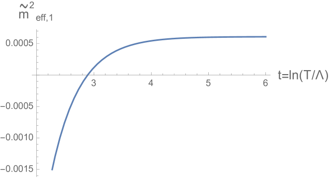
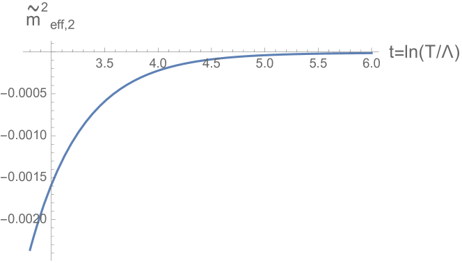
Here $\widetilde{m}_{\text{eff},2}^{2}$ remains negative for all values of $t$. Its magnitude grows as one goes to lower temperatures. At high temperatures, it saturates at a negative value. This means that the baryon symmetry in the second sector remains broken at all temperatures where the perturbative analysis is valid. The behavior of $\widetilde{m}_{\text{eff},1}^{2}$ is quite similar to that of $\widetilde{m}_{\text{eff},2}^{2}$ in the low temperature regime, i.e., in this regime $\widetilde{m}_{\text{eff},1}^{2}<0$ and $|\widetilde{m}_{\text{eff},1}^{2}|$ grows as the temperature is lowered. However, at high temperatures $\widetilde{m}_{\text{eff},1}^{2}$ saturates at a positive value. This means that the baryon symmetry in the first sector is restored at a critical temperature. The value of of this critical temperature ($T_{c}$) is given by $t_{c}=\ln(T_{c}/\Lambda)\approx 2.889$.

4.2 Case 2: $M_{1}^{2}=0,M_{2}^{2}\neq 0$

In this case the expressions of the rescaled effective masses (squared) are

$$\begin{split}&\widetilde{m}_{\text{eff},1}^{2}=(1+\sin\theta)c_{2}\ e^{-(2-8R_{0})t}+R_{0}\Big{(}r\cos\theta+\sin\theta\Big{)}+\frac{3}{4}\lambda,\\ &\widetilde{m}_{\text{eff},2}^{2}=\frac{1}{r}\cos\theta\ c_{2}\ e^{-(2-8R_{0})t}+R_{0}\Big{(}\frac{\cos\theta}{r}-\sin\theta\Big{)}+\frac{3}{4}\lambda.\end{split}$$ (53)

As we have noted earlier, $\cos\theta<0$ for the systems that we are considering, and $(1+\sin\theta)>0$ for all values of $\theta$ in this domain. Therefore, at sufficiently low temperatures, when the renormalized masses (squared) dominate over the thermal masses (squared), $\widetilde{m}_{\text{eff},1}^{2}$ and $\widetilde{m}_{\text{eff},2}^{2}$ have opposite signs. These signs depends on whether $c_{2}$ (or equivalently, $M_{2}^{2}$) is positive or negative.

4.2.1 Subcase 1: $M_{2}^{2}>0$

When $M_{2}^{2}>0$, i.e., $c_{2}>0$, then $\widetilde{m}_{\text{eff},1}^{2}>0$ and $\widetilde{m}_{\text{eff},2}^{2}<0$ in the low temperature regime. This means that in this regime the baryon symmetry in the first sector remains unbroken and the baryon symmetry in the second sector is spontaneously broken. This is identical to the phase in the high temperature limit. Therefore, we expect the system to remain in the same phase at all temperatures in the domain of validity of the perturbative analysis. To verify this we plot $\widetilde{m}_{\text{eff},1}^{2}$ and $\widetilde{m}_{\text{eff},2}^{2}$ at different temperatures for $r=0.1$, $\theta=\pi$, $\lambda=0.001$, $c_{1}=0$ and $c_{2}=0.1$ in figure 11. We can see that $\widetilde{m}_{\text{eff},1}^{2}>0$ and $\widetilde{m}_{\text{eff},2}^{2}<0$ for all values of $t$. This indicates that the system remains in the same phase at all temperatures where perturbation theory can be trusted.

Figure 11: Plots of the rescaled effective masses (squared) against $t=\ln(T/\Lambda)$ for $r=0.1$, $\theta=\pi$, $\lambda=0.001$, $c_{1}=0$, $c_{2}=0.1$: $\widetilde{m}_{\text{eff},1}^{2}>0$ and $\widetilde{m}_{\text{eff},2}^{2}<0$ at all temperatures indicating the absence of any phase transition in the domain of validity of the perturbative analysis.

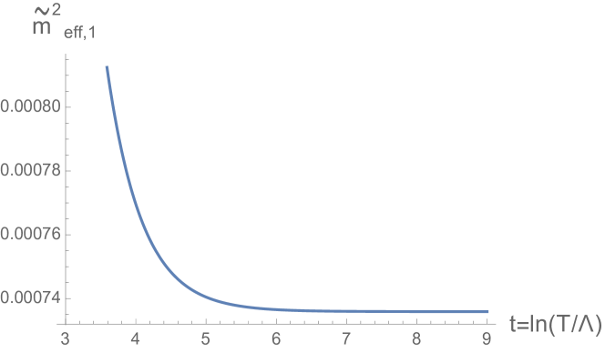
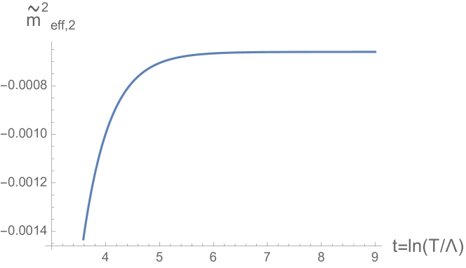
4.2.2 Subcase 2: $M_{2}^{2}<0$

When $M_{2}^{2}<0$, i.e., $c_{2}<0$, then $\widetilde{m}_{\text{eff},1}^{2}<0$ and $\widetilde{m}_{\text{eff},2}^{2}>0$ in the low temperature regime. This means that in this regime the baryon symmetry in the first sector is spontaneously broken and the baryon symmetry in the second sector is unbroken. On the other hand, in the high temperature limit, as we have already seen, the baryon symmetry in the first sector is unbroken and the baryon symmetry in the second sector is spontaneously broken. Therefore, as one goes from the low temperature regime to the high temperature regime, the baryon symmetry in the first sector would be restored at some critical temperature $T_{c1}$ and the baryon symmetry in the second sector would be broken at a possibly different critical temperature $T_{c2}$. At these two critical temperatures,

$$|m_{1}^{2}|_{\mu=T_{c1}}|\sim\frac{16\pi^{2}}{3}\lambda T_{c1}^{2}\ll T_{c1}^{2},\ |m_{2}^{2}|_{\mu=T_{c2}}|\sim\frac{16\pi^{2}}{3}\lambda T_{c2}^{2}\ll T_{c2}^{2}.$$ (54)

From the relation between the two renormalized masses (squared), we get

$$|m_{2}^{2}|_{\mu=T_{c1}}|=\frac{|m_{1}^{2}|_{\mu=T_{c1}}|}{\widetilde{\alpha}},\ |m_{1}^{2}|_{\mu=T_{c2}}|=\widetilde{\alpha}|m_{2}^{2}|_{\mu=T_{c2}}|$$ (55)

where $\widetilde{\alpha}\equiv-\frac{r(1+\sin\theta)}{\cos\theta}$. Just like $\alpha$ in the previous case, $\widetilde{\alpha}<1$ in the domain $r<r_{\text{max}}$ and $\theta\in(\theta_{1},\theta_{2})$ as can be seen from the plot given in figure 12. Therefore,

$$|m_{1}^{2}|_{\mu=T_{c2}}|\lesssim\frac{16\pi^{2}}{3}\lambda T_{c2}^{2}\ll T_{c2}^{2}.$$ (56)

Figure 12: Plot of $\widetilde{\alpha}=-\frac{r(1+\sin\theta)}{\cos\theta}$ against $r$ and $\theta$ in the domain $r<r_{\text{max}}$ and $\theta\in(\theta_{1},\theta_{2})$.

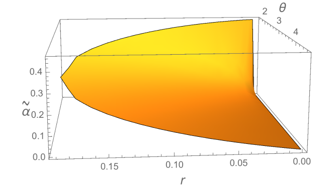
Note that $|m_{i}^{2}|_{\mu=T_{c2}}|\ll T_{c2}^{2}$ means that the expressions of the thermal masses (squared) given in (38) are reliable near the critical temperature $T_{c2}$. $|m_{1}^{2}|_{\mu=T_{c2}}|\lesssim\frac{16\pi^{2}}{3}\lambda T_{c2}^{2}$ further implies that near the critical temperature $T_{c2}$, $m_{\text{eff},1}^{2}$ satisfies the condition

$$|m_{\text{eff},1}^{2}|\sim\frac{16\pi^{2}}{3}\lambda T^{2}.$$ (57)

This means that we can rely on the perturbative analysis with $\mu=T$ in this regime.

Near the other critical temperature ($T_{c1}$) the perturbative analysis can break down if $\widetilde{\alpha}$ is very small. To avoid this, we choose a system where $r=0.1$ and $\theta=2.1$ for which $\widetilde{\alpha}\approx 0.369$. In this system, we have

$$|m_{2}^{2}|_{\mu=T_{c1}}|\approx 2.71|m_{1}^{2}|_{\mu=T_{c1}}|\sim\frac{16\pi^{2}}{3}\lambda T_{c1}^{2}.$$ (58)

Therefore, in this case we can rely on the perturbative analysis even near the critical temperature $T_{c1}$. In figure 13 we provide the plots of the rescaled effective masses (squared) against $t=\ln(T/\Lambda)$ for $r=0.1$, $\theta=2.1$, $\lambda=0.001$, $c_{1}=0$ and $c_{2}=-0.1$.

Figure 13: Plots of the rescaled effective masses (squared) against $t=\ln(T/\Lambda)$ for $r=0.1$, $\theta=2.1$, $\lambda=0.001$, $c_{1}=0$, $c_{2}=-0.1$: $\widetilde{m}_{\text{eff},1}^{2}<0$ and $\widetilde{m}_{\text{eff},2}^{2}>0$ in the low temperature regime. In the high temperature limit, $\widetilde{m}_{\text{eff},1}^{2}$ saturates at a positive value while $\widetilde{m}_{\text{eff},2}^{2}$ saturates at a negative value. This indicates that as the temperature is increased, there are two phase transitions. The first phase transition corresponds to the restoration of the baryon symmetry in the first sector. At the second phase transition, the baryon symmetry in the second sector is spontaneously broken. The two critical temperatures $T_{c1}$ and $T_{c2}$ are given by $t_{c1}=\ln(T_{c1}/\Lambda)\approx 2.688$ and $t_{c2}=\ln(T_{c2}/\Lambda)\approx 4.355$.

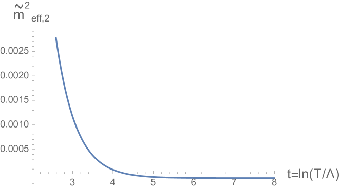
As we can see from these plots, $\widetilde{m}_{\text{eff},1}^{2}$ and $\widetilde{m}_{\text{eff},2}^{2}$ both flip their signs as the temperature is increased. The critical temperatures ($T_{c1}$ and $T_{c2}$) corresponding to these phase transitions are given by $t_{c1}=\ln(T_{c1}/\Lambda)\approx 2.688$ and $t_{c2}=\ln(T_{c2}/\Lambda)\approx 4.355$.

Since the perturbative analysis with $\mu=T$ is valid near the critical temperature $T_{c2}$ for different values of $(r,\theta)$ in the domain $r<r_{\text{max}}$, $\theta\in(\theta_{1},\theta_{2})$, we can provide a general expression for $T_{c2}$. This critical temperature can be evaluated by demanding that $\widetilde{m}_{\text{eff},2}^{2}=0$ at $T=T_{c2}$. This gives us the following expression for $t_{c2}\equiv\ln(T_{c2}/\Lambda)$:

$$\begin{split}&t_{c2}=-\frac{1}{2-8R_{0}}\ln\Bigg{[}-\frac{r}{c_{2}\cos\theta}\Bigg{\{}R_{0}\Big{(}\frac{\cos\theta}{r}-\sin\theta\Big{)}+\frac{3}{4}\lambda\Bigg{\}}\Bigg{]}.\end{split}$$ (59)

In figure 14, we plot $t_{c2}$ against $\theta$ in the domain $\theta\in(\theta_{1},\theta_{2})$ for $r=0.1$, $\lambda=0.001$, $c_{1}=0$ and $c_{2}=-0.1$.

Figure 14: Plot of $t_{c2}$ against $\theta$ for $r=0.1,\ \lambda=0.001,\ c_{1}=0,\ c_{2}=-0.1$: $t_{c2}\rightarrow\infty$ as $\theta\rightarrow\theta_{1}$ or $\theta\rightarrow\theta_{2}$.

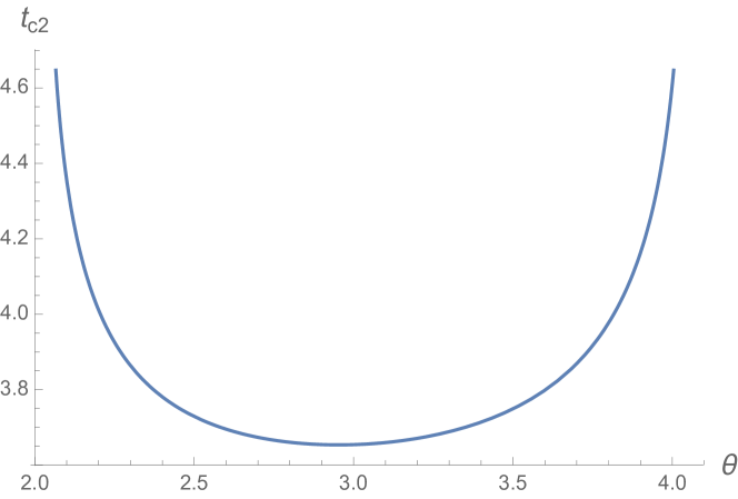
From this plot, we can see that $t_{c2}$ increases sharply as one approaches the edges of the domain $(\theta_{1},\theta_{2})$, and $t_{c2}\rightarrow\infty$ as $\theta\rightarrow\theta_{1}$ or $\theta\rightarrow\theta_{2}$. This means that at these edges, the baryon symmetries in the second sector remains unbroken at all temperatures where the perturbative analysis is valid.

4.3 Summary of the results and comments on the case $M_{1}^{2}\neq 0,\ M_{2}^{2}\neq 0$

In this section we studied the systems that are obtained by introducing masses to the scalar fields in the RDB model. We restricted our attention to the systems that flow to the UV fixed points exhibiting thermal order in the second sector. Due to this behavior of the systems in the UV regime, these systems remain in a persistently symmetry-broken phase in the high temperature limit. We found that as the temperature is lowered, the effects of the renormalized masses of the scalar fields start becoming significant. At sufficiently low temperatures, these renormalized masses can lead to phase transitions in the system. We studied such phase transitions for different values of two mass² scales $M_{1}^{2}$ and $M_{2}^{2}$ that appear in the renormalized masses (squared). When both these scales are nonzero, they determine the asymptotic behavior of the renormalized masses (squared) in the IR and UV regimes respectively. However, to simplify the analysis, we considered the following two cases where only one of these scales is nonzero:

1. $M_{1}^{2}\neq 0,M_{2}^{2}=0$,

2. $M_{1}^{2}=0,M_{2}^{2}\neq 0$.

We showed that in each of these cases, the sign of the nonzero $M_{i}^{2}$ determines the phase transitions occurring in the system. We showed that in certain parameter regimes, one can study these phase transitions using perturbation theory with the renormalization scale $\mu=T$. In these regimes, the perturbation theory remains valid slightly below the critical temperatures corresponding to the phase transitions. We called the phases at these scales the ‘low temperature’ phases of the systems. These low temperature phases and the associated phase transitions for the different cases are summarized in table 1.

Table 1: Phase transitions for the systems in which the baryon symmetry in the first sector is unbroken and the baryon symmetry in the second sector is broken at the high temperature limit.

	Fate of the baryon symmetry		Phase transitions as the
$M_{1}^{2},\ M_{2}^{2}$	in the low temperature regime		temperature is increased
	First sector	Second sector
			Baryon symmetry in the
$M_{1}^{2}>0,\ M_{2}^{2}=0$	unbroken	unbroken	second sector is broken
			at a critical temperature.
			Baryon symmetry in the
$M_{1}^{2}<0,\ M_{2}^{2}=0$	broken	broken	first sector is restored
			at a critical temperature.
$M_{1}^{2}=0,\ M_{2}^{2}>0$	unbroken	broken	No phase transition.
			2 phase transitions:
			At a critical temperature $T_{c1}$
			baryon symmetry in the
$M_{1}^{2}=0,\ M_{2}^{2}<0$	broken	unbroken	first sector is restored.
			At another critical temperature
			$T_{c2}$, baryon symmetry in the
			second sector is broken.

We expect similar phase transitions even outside the aforementioned parameter regimes. However, to be sure of this, one would need to improve the perturbative analysis which lies beyond the scope of this paper.

Finally, let us end this section by commenting on the possible phase structures when both $M_{1}^{2}$ and $M_{2}^{2}$ are nonzero. In general, it is hard to ascertain the regime of validity of the perturbative analysis near the critical temperatures in these cases. So, the following discussion will be mostly speculative. In the presence of both $M_{1}^{2}$ and $M_{2}^{2}$, we expect the sign of $M_{1}^{2}$ to determine the phase in the low temperature regime. This is due to the fact that as the temperature is lowered, the terms with the coefficient $c_{1}\equiv\frac{3M_{1}^{2}}{32\pi^{2}\Lambda^{2}}$ in the rescaled effective masses (squared) given in (43) grow faster than the terms with the coefficient $c_{2}\equiv\frac{3M_{2}^{2}}{32\pi^{2}\Lambda^{2}}$. However, at intermediate temperatures the phase can depend on $M_{2}^{2}$ as well. The situations in which $M_{2}^{2}$ can play an important role in determining the phase at such intermediate temperature scales can be guessed from the low temperature phases in the presence of a single $M_{i}^{2}$ that are given in table 1. If the signs of $M_{1}^{2}$ and $M_{2}^{2}$ are such that individually both of them lead to the same phase in a sector at low temperatures, then the phases in that sector at different temperature regimes would be identical to those in the presence of $M_{1}^{2}$ alone. On the other hand, if the signs of $M_{1}^{2}$ and $M_{2}^{2}$ are such that individually they lead to distinct phases in a sector at low temperatures, then there are the following two possibilities. If there is a phase transition in that sector when only $M_{1}^{2}$ is nonzero, we do not expect anything dramatic to happen in the presence of $M_{2}^{2}$ apart from a modification of the critical temperature corresponding to this phase transition. However, if there is no phase transition in that sector when only $M_{1}^{2}$ is nonzero, then a pair of phase transitions might be induced by the presence of $M_{2}^{2}$. Whether such a pair of phase transitions occurs or not would depend on the relative magnitudes of $M_{1}^{2}$ and $M_{2}^{2}$. In case such phase transitions indeed occur in a particular sector, the phase in that sector between the two critical temperatures would be the same as the low temperature phase in the presence of $M_{2}^{2}$ alone. We do not undertake a detailed study of such double phase transitions as the perturbation theory with $\mu=T$ may not be appropriate for analyzing the phases near the two critical temperatures.

To illustrate the possibility of such a pair of phase transitions and the associated problems with the perturbative analysis, let us consider a system where $r=0.1$, $\theta=2.1$, $\lambda=0.001$ and $c_{1}=c_{2}=-0.2$. In figure 15 we plot the rescaled effective masses (squared) against $t=\ln(T/\Lambda)$ for this system.

Figure 15: Plots of the rescaled effective masses (squared) against $t=\ln(T/\Lambda)$ for $r=0.1$, $\theta=2.1$, $\lambda=0.001$, $c_{1}=c_{2}=-0.2$: A pair of phase transitions occurs in the second sector.

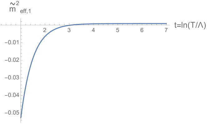
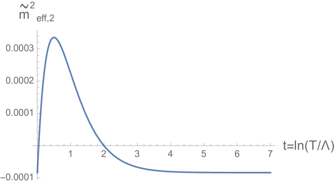
From these plots, we can see that at sufficiently low temperatures, both $\widetilde{m}_{\text{eff},1}^{2}$ and $\widetilde{m}_{\text{eff},2}^{2}$ are negative which indicates that the baryon symmetry in both the sectors are broken in this regime. This behavior at lower temperatures is determined by the negative sign of $M_{1}^{2}$ (see table 1). As the temperature is increased, due to the presence of a negative $M_{2}^{2}$, $\widetilde{m}_{\text{eff},2}^{2}$ becomes positive at a critical temperature indicating the restoration of the baryon symmetry in the second sector. When the temperature is increased further, $\widetilde{m}_{\text{eff},2}^{2}$ again becomes negative at a critical temperature and remains so at higher temperatures. This second phase transition is driven by the thermal mass (squared) $m_{\text{th},2}^{2}$ which begins to dominate over the renormalized mass (squared) $m_{2}^{2}|_{\mu=T}$ in this regime. At this second critical temperature, the system re-enters into a phase where the baryon symmetry in the second sector is spontaneously broken. However, note that $|\widetilde{m}_{\text{eff},1}^{2}|$ becomes much larger than $\lambda$ at temperatures higher than both the critical temperatures mentioned above, i.e., $|m_{\text{eff},1}^{2}|$ no longer remains $O(\frac{16\pi^{2}}{3}\lambda T^{2})$ near these critical temperatures. This indicates that the perturbative analysis with $\mu=T$ is unreliable in these regimes. We hope to come up with a more reliable analysis of such double phase transitions in the future.

5 Conclusion and discussion

In this paper we considered relevant and marginally relevant deformations of the large $N$ CFTs introduced in Chaudhuri:2020xxb and showed that in the $N\rightarrow\infty$ limit, the resulting RG flows end at these CFTs in the UV regime. The gauge groups in these theories have the product form given in (1). This structure of the gauge group implies the existence of two distinct sectors in the models. The ranks of the gauge groups in the two sectors can be unequal. The matter fields in each sector transform in certain representations of the gauge group in that sector while remaining invariant under the gauge transformations in the other sector. In each of these sectors, there is a global $\mathbb{Z}_{2}$ (or $U(1)$) baryon symmetry. It is the fate of these symmetries at different temperatures that was of interest to us in this work. We studied the RG flows of these theories to analyze whether the baryon symmetries in the two sectors are spontaneously broken or not at different temperature scales. As we mentioned above, the UV fixed points of these RG flows are the large $N$ CFTs explored in Chaudhuri:2020xxb . These CFTs are weakly coupled and they lie on a conformal manifold with the shape of a circle in the space of couplings. It was shown in Chaudhuri:2020xxb that when the ratio of the ranks of the gauge groups in the two sectors is sufficiently away from 1, an angular interval on this circle of fixed points demonstrates thermal order characterized by the spontaneous breaking of the $\mathbb{Z}_{2}$ (or $U(1)$) global baryon symmetry in the sector with the smaller gauge group. It was also shown that this symmetry breaking is accompanied by the Higgsing of half of the gauge bosons in the same sector at all nonzero temperatures. From these facts, we concluded that the systems described by the RG flows ending at these UV fixed points exhibit a symmetry-broken phase in the high temperature regime. We studied the IR limits of the RG flows corresponding to the different deformations and found interesting patterns of phase transitions. Let us summarize the features of these phase transitions for the different deformations below.

The first class of deformations that we considered involved variations of the double trace quartic couplings of the scalar fields from their values on the fixed circle. We showed that for each point on the fixed circle there is a marginally relevant deformation belonging to this class. The RG flows triggered by these marginally relevant deformations lead to a weakly coupled fixed point in the IR where the two sectors are decoupled. In fact, the theories remain weakly coupled throughout these RG flows. At the IR fixed point of these flows, the baryon symmetries in both the sectors are unbroken at any nonzero temperature. On the other hand, as mentioned earlier, the UV fixed points for some of these flows demonstrate thermal order characterized by spontaneous breaking of the baryon symmetry in the sector with the smaller gauge group. We showed that for each of these flows, there is an inverse symmetry breaking at a critical temperature where the baryon symmetry in the sector with the smaller gauge group is spontaneously broken. We determined this critical temperature by finding the temperature scale at which the thermal mass of the scalar fields in the respective sector goes to zero.

The second class of deformations involved adding masses to the scalar fields while keeping all the couplings in the model frozen at a fixed point which exhibits thermal order in the smaller sector. We studied the RG flows of these masses. This analysis showed that there are two mass² scales, $M_{1}^{2}$ and $M_{2}^{2}$, which determine the asymptotic behavior of the renormalized masses (squared) in the IR and the UV regimes respectively when both of them are nonzero. We found that in the high temperature limit, the effects of both these scales are suppressed compared to those of the thermal masses (squared) of the scalar fields, and the system remains in the same phase as the UV fixed point. Therefore, the baryon symmetry in the smaller sector remains persistently broken in this regime. The baryon symmetry in the larger sector, on the other hand, is unbroken in the same regime. As the temperature is lowered, the effects of $M_{1}^{2}$ and $M_{2}^{2}$ start becoming significant. At sufficiently low temperatures, they can induce phase transitions in the system. The nature of these phase transitions depends on the magnitudes and signs of $M_{1}^{2}$ and $M_{2}^{2}$. We did a detailed analysis of these phase transitions for the cases where only one of the $M_{i}^{2}$’s is nonzero. The results of this analysis for the systems where the second sector has the smaller gauge group are summarized in table 1. We also found that when both $M_{1}^{2}$ and $M_{2}^{2}$ are nonzero, in some cases there may be a pair of phase transitions occurring in a sector at different critical temperatures. We discussed the limitations of our perturbative analysis in studying the detailed features of such double phase transitions and estimating the corresponding critical temperatures.

We now comment on a few subtleties in the analysis done in this work. Firstly, note that we relied on the 1-loop expressions of the beta functions and the thermal masses to determine the phases at different temperatures. We expect the higher loop corrections to refine the estimates of the critical temperatures while not changing the qualitative features of the phases in the different regimes. In this context, it is also important to remember that thermal perturbation theory is riddled with infrared problems Linde:1980ts ; Gross:1980br . In the models that we considered there are three mass scales at any temperature $T$ where we could employ the perturbative analysis. These three mass scales are associated with the following modes:

1. The “hard” nonzero Matsubara modes of the different fields; these modes have masses of the order of $\pi T$,

2. The “soft” zero Matsubara modes of the scalar fields and the longitudinal gauge bosons; these modes have masses of the order of $\sqrt{\frac{16\pi^{2}}{3}\lambda}T$,

3. The “ultrasoft” zero Matsubara modes of the un-Higgsed transverse gauge bosons; these modes have masses of the order of $\frac{16\pi^{2}}{3}\lambda T$.

The different phases in our models are determined by the physics at the soft scale while the IR problems arise from the ultrasoft modes. They appear in the form of an infinite number of diagrams at a subleading order in the effective potential. This leads to breakdown of perturbation theory at this order. Usually this non-perturbative physics is studied by employing the dimensionally reduced effective theory framework and the techniques of lattice gauge theories Laine:2016hma ; Farakos:1994kx ; Kajantie:1995kf ; Kajantie:1996qd ; Moore:2000jw ; Kainulainen:2019kyp ; Gould:2019qek ; Niemi:2020hto . Such studies on a variety of models indicate that these non-perturbative contributions typically do not alter the qualitative features of the phases in different regimes. We expect a similar thing in the models considered in this paper. It may be useful to check this explicitly in the future.

Another point to which we would like to draw the reader’s attention is that the UV fixed points of the RG flows studied in this paper are like the Banks-Zaks-Caswell fixed points in more familiar QFTs. Such fixed points are typically considered to be IR fixed points as small variations of the gauge couplings from their values at these fixed points usually lead to asymptotic freedom. In our analysis, we avoided this by fixing the gauge couplings (as well as the single trace quartic couplings) at their fixed point values. This could be done in the massive theories that we considered in section 4 because the RG flows of the masses do not backreact on the flows of the gauge couplings (as well as the quartic couplings) in the $\overline{\text{MS}}$ scheme. In case of the massless theories considered in section 3, the single trace couplings could be kept frozen at their fixed point values as their beta functions are independent of the double trace couplings at the planar limit Chaudhuri:2020xxb .

Finally, let us end with some comments on how finite $N$ corrections may alter the features that we have presented at the planar limit. Currently, it is not clear to us whether the UV fixed points lying on the conformal manifold survive under such corrections. We refer the reader to the analysis in appendix H of Chaudhuri:2020xxb for some perturbative computations of $1/N$ corrections which suggest that these fixed points may survive under such corrections. Another potential problem would arise at finite N due to the fact that the double trace couplings start affecting the RG flows of the single trace couplings. This can eventually drive these couplings away from their planar fixed point values at sufficiently high temperatures where the cumulative effects of $1/N$ corrections become significant. Resolving both the issues mentioned above is complicated by the fact that to take into account $1/N$ corrections while staying in a regime where $1/N\ll$ ’t Hooft couplings, one would need to re-sum the perturbative expansions in the ’t Hooft couplings. It would be interesting to explore whether the thermal order persists under $1/N$ corrections after such re-summations. We would like to return to these issues in the future.

Appendix A Positivity of the quartic terms in the thermal effective potential at leading order

In this appendix we will show that the tree-level quartic terms in the thermal effective potential of the scalar fields remain positive throughout the RG flows studied in section 3.2. These quartic terms have the following form:

$$V_{\text{quartic}}=16\pi^{2}\Bigg{[}\sum_{i=1}^{2}\frac{h_{i}}{N_{ci}}\text{Tr}[\rho_{i}^{2}]+\sum_{i=1}^{2}\frac{f_{i}}{N_{ci}^{2}}\Big{(}\text{Tr}[\rho_{i}]\Big{)}^{2}+\frac{2\zeta}{N_{c1}N_{c2}}\text{Tr}[\rho_{1}]\text{Tr}[\rho_{2}]\Bigg{]},$$ (60)

where $\rho_{i}\equiv\Phi_{i}^{T}\Phi_{i}$. Note that $\rho_{1}$ and $\rho_{2}$ are positive-definite matrices. From this one can easily see that a sufficient condition for the positivity of $V_{\text{quartic}}$ is

$$h_{i}>0,\ f_{i}>0,\ f_{1}f_{2}-\zeta^{2}>0.$$ (61)

Let us now check whether these inequalities are satisfied throughout the above-mentioned RG flows. Firstly, let us note that $h_{1}$ and $h_{2}$ are frozen at the following common value in these RG flows:

$$h_{1}=h_{2}=h=\Big{(}\frac{3-\sqrt{6}}{16}\Big{)}\lambda.$$ (62)

Since $\lambda$ and the coefficient $\Big{(}\frac{3-\sqrt{6}}{16}\Big{)}$ are both positive, we can see that $h>0$. Now, let us look at the double trace couplings $f_{1}=f_{p}+R\sin\theta$ and $f_{2}=f_{p}-R\sin\theta$. The values of $f_{p}$ and $R$ along these RG flows are as follows.

$$\begin{split}&f_{p}=f_{0p}+\frac{R_{0}}{2}\Bigg{[}\frac{(1-k)\Big{(}1-\tanh(8R_{0}t)\Big{)}}{1+k\tanh(8R_{0}t)}\Bigg{]}\ ,\ R=\frac{R_{0}}{2}\Bigg{[}\frac{(1+k)\Big{(}1+\tanh(8R_{0}t)\Big{)}}{1+k\tanh(8R_{0}t)}\Bigg{]}\ .\end{split}$$ (63)

From these values of the couplings along the RG flow, we get

$$\begin{split}&f_{1,2}=f_{p}\pm R\sin\theta\geq f_{p}-R=f_{0p}-R_{0}+(1-k)R_{0}\Bigg{[}\frac{1-\tanh(8R_{0}t)}{1+k\tanh(8R_{0}t)}\Bigg{]}.\end{split}$$ (64)

Here the quantities $k$ and $\tanh(8R_{0}t)$ satisfy the following inequalities:

$$0<k<1,\ -1<\tanh(8R_{0}t)<1.$$ (65)

From this, we can infer that

$$\begin{split}&(1-k)R_{0}\Bigg{[}\frac{1-\tanh(8R_{0}t)}{1+k\tanh(8R_{0}t)}\Bigg{]}>0.\end{split}$$ (66)

This leads to the positivity of the couplings $f_{1}$ and $f_{2}$ as shown below:

$$\begin{split}&f_{1,2}>f_{0p}-R_{0}=\Bigg{[}\frac{\sqrt{6}}{8}-\frac{\sqrt{18\sqrt{6}-39}}{16}\Bigg{]}\lambda\approx 0.165\lambda>0.\end{split}$$ (67)

Note that for $\theta=\frac{\pi}{2}$ the positivity of $f_{1}$ and $f_{2}$ implies

$$\begin{split}&f_{p}\pm R>0.\end{split}$$ (68)

This also leads to the positivity of the quantity $(f_{1}f_{2}-\zeta^{2})$ as shown below:

$$\begin{split}&f_{1}f_{2}-\zeta^{2}=f_{p}^{2}-R^{2}=(f_{p}+R)(f_{p}-R)>0.\end{split}$$ (69)

Therefore, we have shown that all the conditions given in (61) are satisfied by the couplings throughout the RG flows discussed in section 3.2. Therefore the corresponding tree-level quartic terms in the thermal effective potential of the scalar fields are positive-definite.

Appendix B RG flows of the masses of the scalar fields

In this appendix we will derive the RG flows of the masses of the scalar fields that were introduced in section 4. For this we will rely on the expressions of the 1-loop beta functions of such masses in a general gauge theory given in Luo:2002ti . To be able to use these expressions, we need to re-express the quadratic and quartic terms involving the scalar fields in the Lagrangian of the RDB model as follows:

$$\mathcal{L}_{\text{mass}}=-\frac{1}{2}\overline{m}^{2}_{a_{r}i_{r},b_{s}j_{s}}(\Phi_{r})_{a_{r}i_{r}}(\Phi_{s})_{b_{s}j_{s}},$$ (70)

$$\mathcal{L}_{\text{quartic}}=-\frac{1}{4!}\overline{\lambda}_{a_{r}i_{r},b_{s}j_{s},c_{t}k_{t},d_{u}l_{u}}(\Phi_{r})_{a_{r}i_{r}}(\Phi_{s})_{b_{s}j_{s}}(\Phi_{t})_{c_{t}k_{t}}(\Phi_{u})_{d_{u}l_{u}}$$

where $\overline{m}^{2}_{a_{r}i_{r},b_{s}j_{s}}$ and $\overline{\lambda}_{a_{r}i_{r},b_{s}j_{s},c_{t}k_{t},d_{u}l_{u}}$ are symmetric under exchange of indices. By comparing the above forms with those given in (32) and (2), we can see that

$$\begin{split}&\overline{m}^{2}_{a_{1}i_{1},b_{1}j_{1}}\equiv m_{1}^{2}\delta_{a_{1}b_{1}}\delta_{i_{1}j_{1}},\ \overline{m}^{2}_{a_{2}i_{2},b_{2}j_{2}}\equiv m_{2}^{2}\delta_{a_{2}b_{2}}\delta_{i_{2}j_{2}},\ \overline{m}^{2}_{a_{1}i_{1},b_{2}j_{2}}=\overline{m}^{2}_{a_{2}i_{2},b_{1}j_{1}}\equiv 0,\end{split}$$ (71)

$$\begin{split}\overline{\lambda}_{a_{1}i_{1},b_{1}j_{1},c_{1}k_{1},d_{1}l_{1}}\equiv&4\widetilde{h}_{1}\Bigg{[}\delta_{i_{1}j_{1}}\delta_{k_{1}l_{1}}(\delta_{a_{1}c_{1}}\delta_{b_{1}d_{1}}+\delta_{a_{1}d_{1}}\delta_{b_{1}c_{1}})+\delta_{i_{1}k_{1}}\delta_{j_{1}l_{1}}(\delta_{a_{1}b_{1}}\delta_{c_{1}d_{1}}+\delta_{a_{1}d_{1}}\delta_{b_{1}c_{1}})\\ &\quad+\delta_{i_{1}l_{1}}\delta_{j_{1}k_{1}}(\delta_{a_{1}b_{1}}\delta_{c_{1}d_{1}}+\delta_{a_{1}c_{1}}\delta_{b_{1}d_{1}})\Bigg{]}\\ &+8\widetilde{f}_{1}\Bigg{[}\delta_{i_{1}j_{1}}\delta_{k_{1}l_{1}}\delta_{a_{1}b_{1}}\delta_{c_{1}d_{1}}+\delta_{i_{1}k_{1}}\delta_{j_{1}l_{1}}\delta_{a_{1}c_{1}}\delta_{b_{1}d_{1}}+\delta_{i_{1}l_{1}}\delta_{j_{1}k_{1}}\delta_{a_{1}d_{1}}\delta_{b_{1}c_{1}}\Bigg{]},\end{split}$$ (72)

$$\begin{split}\overline{\lambda}_{a_{2}i_{2},b_{2}j_{2},c_{2}k_{2},d_{2}l_{2}}\equiv&4\widetilde{h}_{2}\Bigg{[}\delta_{i_{2}j_{2}}\delta_{k_{2}l_{2}}(\delta_{a_{2}c_{2}}\delta_{b_{2}d_{2}}+\delta_{a_{2}d_{2}}\delta_{b_{2}c_{2}})+\delta_{i_{2}k_{2}}\delta_{j_{2}l_{2}}(\delta_{a_{2}b_{2}}\delta_{c_{2}d_{2}}+\delta_{a_{2}d_{2}}\delta_{b_{2}c_{2}})\\ &\quad+\delta_{i_{2}l_{2}}\delta_{j_{2}k_{2}}(\delta_{a_{2}b_{2}}\delta_{c_{2}d_{2}}+\delta_{a_{2}c_{2}}\delta_{b_{2}d_{2}})\Bigg{]}\\ &+8\widetilde{f}_{2}\Bigg{[}\delta_{i_{2}j_{2}}\delta_{k_{2}l_{2}}\delta_{a_{2}b_{2}}\delta_{c_{2}d_{2}}+\delta_{i_{2}k_{2}}\delta_{j_{2}l_{2}}\delta_{a_{2}c_{2}}\delta_{b_{2}d_{2}}+\delta_{i_{2}l_{2}}\delta_{j_{2}k_{2}}\delta_{a_{2}d_{2}}\delta_{b_{2}c_{2}}\Bigg{]},\end{split}$$ (73)

$$\begin{split}&\overline{\lambda}_{a_{1}i_{1},b_{1}j_{1},c_{2}k_{2},d_{2}l_{2}}=\overline{\lambda}_{a_{1}i_{1},c_{2}k_{2},b_{1}j_{1},d_{2}l_{2}}=\overline{\lambda}_{a_{1}i_{1},c_{2}k_{2},d_{2}l_{2},b_{1}j_{1}}\\ &=\overline{\lambda}_{c_{2}k_{2},a_{1}i_{1},b_{1}j_{1},d_{2}l_{2}}=\overline{\lambda}_{c_{2}k_{2},a_{1}i_{1},d_{2}l_{2},b_{1}j_{1}}=\overline{\lambda}_{c_{2}k_{2},d_{2}l_{2},a_{1}i_{1},b_{1}j_{1}}\equiv 8\widetilde{\zeta}\delta_{a_{1}b_{1}}\delta_{i_{1}j_{1}}\delta_{c_{2}d_{2}}\delta_{k_{2}l_{2}}.\end{split}$$ (74)

Now, we can use the expressions given in Luo:2002ti to get the following 1-loop beta functions of $\overline{m}^{2}_{a_{r}i_{r},b_{s}j_{s}}$:

$$\begin{split}&(4\pi)^{2}\mu\frac{d}{d\mu}(\overline{m}^{2}_{a_{1}i_{1},b_{1}j_{1}})=\overline{m}^{2}_{c_{1}k_{1},d_{1}l_{1}}\overline{\lambda}_{a_{1}i_{1},b_{1}j_{1},c_{1}k_{1},d_{1}l_{1}}+\overline{m}^{2}_{c_{2}k_{2},d_{2}l_{2}}\overline{\lambda}_{a_{1}i_{1},b_{1}j_{1},c_{2}k_{2},d_{2}l_{2}}\\ &\qquad\qquad\qquad\qquad\qquad-3\sum_{r,\gamma=1}^{2}g_{r}^{2}\Lambda^{S,r\gamma}_{a_{1}i_{1},b_{1}j_{1}},\\ &(4\pi)^{2}\mu\frac{d}{d\mu}(\overline{m}^{2}_{a_{2}i_{2},b_{2}j_{2}})=\overline{m}^{2}_{c_{2}k_{2},d_{2}l_{2}}\overline{\lambda}_{a_{2}i_{2},b_{2}j_{2},c_{2}k_{2},d_{2}l_{2}}+\overline{m}^{2}_{c_{1}k_{1},d_{1}l_{1}}\lambda_{a_{2}i_{2},b_{2}j_{2},c_{1}k_{1},d_{1}l_{1}}\\ &\qquad\qquad\qquad\qquad\qquad-3\sum_{r,\gamma=1}^{2}g_{r}^{2}\Lambda^{S,r\gamma}_{a_{2}i_{2},b_{2}j_{2}}.\end{split}$$ (75)

Here

$$\Lambda^{S,r\gamma}_{a_{1}i_{1},b_{1}j_{1}}\equiv 2C_{2}^{r\gamma}(S_{1})\overline{m}^{2}_{a_{1}i_{1},b_{1}j_{1}},\ \Lambda^{S,r\gamma}_{a_{2}i_{2},b_{2}j_{2}}\equiv 2C_{2}^{r\gamma}(S_{2})\overline{m}^{2}_{a_{2}i_{2},b_{2}j_{2}},$$ (76)

where $C_{2}^{r\gamma}(S_{i})$ is the quadratic Casimir of the representation in which the scalar fields in the $i^{th}$ sector transform under the $\gamma^{\text{th}}$ $G_{r}$ in the $r^{\text{th}}$ sector. The values of these quadratic Casimirs are as follows:

$$\begin{split}C_{2}^{r\gamma}(S_{1})=\delta_{r1}\Big{(}\frac{N_{cr}-1}{4}\Big{)},\ C_{2}^{r\gamma}(S_{2})=\delta_{r2}\Big{(}\frac{N_{cr}-1}{4}\Big{)}.\end{split}$$ (77)

Substituting these quadratic Casimirs as well as the parameters $\overline{m}^{2}_{a_{r}i_{r},b_{s}j_{s}}$ and $\overline{\lambda}_{a_{r}i_{r},b_{s}j_{s},c_{t}k_{t},d_{u}l_{u}}$ by their values given above, and then switching to the ’t Hooft couplings introduced in (3), we get

$$\begin{split}&\mu\frac{dm_{1}^{2}}{d\mu}=8\Bigg{[}h_{1}\Bigg{(}2+\frac{1}{N_{c1}}\Bigg{)}+f_{1}\Bigg{(}1+\frac{2}{N_{c1}^{2}}\Bigg{)}\Bigg{]}m_{1}^{2}+8\zeta\frac{N_{c2}}{N_{c1}}m_{2}^{2}-3\lambda_{1}\Bigg{(}1-\frac{1}{N_{c1}}\Bigg{)}m_{1}^{2},\\ &\mu\frac{dm_{2}^{2}}{d\mu}=8\Bigg{[}h_{2}\Bigg{(}2+\frac{1}{N_{c2}}\Bigg{)}+f_{2}\Bigg{(}1+\frac{2}{N_{c2}^{2}}\Bigg{)}\Bigg{]}m_{2}^{2}+8\zeta\frac{N_{c1}}{N_{c2}}m_{1}^{2}-3\lambda_{2}\Bigg{(}1-\frac{1}{N_{c2}}\Bigg{)}m_{2}^{2}.\end{split}$$ (78)

At the planar limit ($N_{c1},N_{c2}\rightarrow\infty$), these beta functions reduce to

$$\begin{split}&\mu\frac{dm_{1}^{2}}{d\mu}=\Big{(}16h_{1}+8f_{1}-3\lambda_{1}\Big{)}m_{1}^{2}+8r\zeta m_{2}^{2},\\ &\mu\frac{dm_{2}^{2}}{d\mu}=\Big{(}16h_{2}+8f_{2}-3\lambda_{2}\Big{)}m_{2}^{2}+\frac{8\zeta}{r}m_{1}^{2},\end{split}$$ (79)

where $r\equiv\frac{N_{c2}}{N_{c1}}$ in the same limit.

References

- (1) S. Chaudhuri, C. Choi and E. Rabinovici, Thermal order in large N conformal gauge theories, JHEP 04 (2021) 203 [2011.13981].
- (2) N. Schupper and N. M. Shnerb, Inverse melting and inverse freezing: A spin model, Phys. Rev. E 72 (2005) 046107.
- (3) S. Weinberg, Gauge and Global Symmetries at High Temperature, Phys. Rev. D9 (1974) 3357.
- (4) J. Orloff, The UV price for symmetry nonrestoration, Phys. Lett. B403 (1997) 309 [hep-ph/9611398].
- (5) G. Bimonte, D. Iniguez, A. Tarancon and C. L. Ullod, Inverse symmetry breaking on the lattice: An Accurate MC study, Nucl. Phys. B559 (1999) 103 [hep-lat/9903027].
- (6) M. B. Pinto and R. O. Ramos, A Nonperturbative study of inverse symmetry breaking at high temperatures, Phys. Rev. D61 (2000) 125016 [hep-ph/9912273].
- (7) R. N. Mohapatra and G. Senjanovic, Soft CP Violation at High Temperature, Phys. Rev. Lett. 42 (1979) 1651.
- (8) P. Langacker and S.-Y. Pi, Magnetic Monopoles in Grand Unified Theories, Phys. Rev. Lett. 45 (1980) 1.
- (9) S. Dodelson and L. M. Widrow, BARYON SYMMETRIC BARYOGENESIS, Phys. Rev. Lett. 64 (1990) 340.
- (10) S. Dodelson, B. R. Greene and L. M. Widrow, Baryogenesis, dark matter and the width of the Z, Nucl. Phys. B372 (1992) 467.
- (11) G. R. Dvali, A. Melfo and G. Senjanovic, Is There a monopole problem?, Phys. Rev. Lett. 75 (1995) 4559 [hep-ph/9507230].
- (12) P. Meade and H. Ramani, Unrestored Electroweak Symmetry, Phys. Rev. Lett. 122 (2019) 041802 [1807.07578].
- (13) Y. Bai, S. J. Lee, M. Son and F. Ye, Global Electroweak Symmetric Vacuum, 2103.09819.
- (14) M. Carena, C. Krause, Z. Liu and Y. Wang, A New Approach to Electroweak Symmetry Non-Restoration, 2104.00638.
- (15) Z. Komargodski, A. Sharon, R. Thorngren and X. Zhou, Comments on Abelian Higgs Models and Persistent Order, SciPost Phys. 6 (2019) 003 [1705.04786].
- (16) K. Aitken, A. Cherman, E. Poppitz and L. G. Yaffe, QCD on a small circle, Phys. Rev. D 96 (2017) 096022 [1707.08971].
- (17) Y. Tanizaki, T. Misumi and N. Sakai, Circle compactification and ’t Hooft anomaly, JHEP 12 (2017) 056 [1710.08923].
- (18) G. V. Dunne, Y. Tanizaki and M. Ünsal, Quantum Distillation of Hilbert Spaces, Semi-classics and Anomaly Matching, JHEP 08 (2018) 068 [1803.02430].
- (19) Z. Wan and J. Wang, Higher anomalies, higher symmetries, and cobordisms III: QCD matter phases anew, Nucl. Phys. B 957 (2020) 115016 [1912.13514].
- (20) S.-I. Hong and J. B. Kogut, Symmetry nonrestoration in a Gross-Neveu model with random chemical potential, Phys. Rev. D 63 (2001) 085014 [hep-th/0007216].
- (21) A. Buchel and C. Pagnutti, Exotic Hairy Black Holes, Nucl. Phys. B 824 (2010) 85 [0904.1716].
- (22) A. Donos and J. P. Gauntlett, Superfluid black branes in AdS_4\times S^7, JHEP 06 (2011) 053 [1104.4478].
- (23) U. Gürsoy, E. Kiritsis, F. Nitti and L. Silva Pimenta, Exotic holographic RG flows at finite temperature, JHEP 10 (2018) 173 [1805.01769].
- (24) A. Buchel, Klebanov-Strassler black hole, JHEP 01 (2019) 207 [1809.08484].
- (25) A. Buchel, Thermal order in holographic CFTs and no-hair theorem violation in black branes, Nucl. Phys. B 967 (2021) 115425 [2005.07833].
- (26) A. Buchel, Holographic conformal order in supergravity, Phys. Lett. B 814 (2021) 136111 [2007.09420].
- (27) A. Buchel, Fate of the conformal order, Phys. Rev. D 103 (2021) 026008 [2011.11509].
- (28) N. Chai, S. Chaudhuri, C. Choi, Z. Komargodski, E. Rabinovici and M. Smolkin, Thermal Order in Conformal Theories, Phys. Rev. D 102 (2020) 065014 [2005.03676].
- (29) N. Chai, S. Chaudhuri, C. Choi, Z. Komargodski, E. Rabinovici and M. Smolkin, Symmetry Breaking at All Temperatures, Phys. Rev. Lett. 125 (2020) 131603.
- (30) M. Hogervorst, S. Rychkov and B. C. van Rees, Unitarity violation at the Wilson-Fisher fixed point in 4- dimensions, Phys. Rev. D 93 (2016) 125025 [1512.00013].
- (31) B. Bajc, A. Lugo and F. Sannino, Asymptotically free and safe fate of symmetry nonrestoration, Phys. Rev. D 103 (2021) 096014 [2012.08428].
- (32) D. F. Litim and F. Sannino, Asymptotic safety guaranteed, JHEP 12 (2014) 178 [1406.2337].
- (33) A. Zee, Study of the renormalization group for small coupling constants, Phys. Rev. D 7 (1973) 3630.
- (34) N. Chai, A. Dymarsky and M. Smolkin, A model of persistent breaking of discrete symmetry, 2106.09723.
- (35) G. Veneziano, Some Aspects of a Unified Approach to Gauge, Dual and Gribov Theories, Nucl. Phys. B 117 (1976) 519.
- (36) M. Bershadsky and A. Johansen, Large N limit of orbifold field theories, Nucl. Phys. B536 (1998) 141 [hep-th/9803249].
- (37) M. Schmaltz, Duality of nonsupersymmetric large N gauge theories, Phys. Rev. D 59 (1999) 105018 [hep-th/9805218].
- (38) A. Dymarsky, I. Klebanov and R. Roiban, Perturbative gauge theory and closed string tachyons, JHEP 11 (2005) 038 [hep-th/0509132].
- (39) A. Dymarsky, I. Klebanov and R. Roiban, Perturbative search for fixed lines in large N gauge theories, JHEP 08 (2005) 011 [hep-th/0505099].
- (40) E. Pomoni and L. Rastelli, Large N Field Theory and AdS Tachyons, JHEP 04 (2009) 020 [0805.2261].
- (41) A. Cherman, M. Hanada and D. Robles-Llana, Orbifold equivalence and the sign problem at finite baryon density, Phys. Rev. Lett. 106 (2011) 091603 [1009.1623].
- (42) M. Hanada and N. Yamamoto, Universality of Phases in QCD and QCD-like Theories, JHEP 02 (2012) 138 [1103.5480].
- (43) G. V. Dunne and M. Ünsal, New Nonperturbative Methods in Quantum Field Theory: From Large-N Orbifold Equivalence to Bions and Resurgence, Ann. Rev. Nucl. Part. Sci. 66 (2016) 245 [1601.03414].
- (44) K. Aitken, C. Choi and A. Karch, New and Old Fermionic Dualities from 3d Bosonization, JHEP 01 (2020) 035 [1909.04036].
- (45) C. B. Jepsen, I. R. Klebanov and F. K. Popov, RG limit cycles and unconventional fixed points in perturbative QFT, Phys. Rev. D 103 (2021) 046015 [2010.15133].
- (46) A. Belavin and A. Migdal, Calculation of anomalous dimensions in non-abelian gauge field theories, Pisma Zh. Eksp. Teor. Fiz. 19 (1974) 317.
- (47) W. E. Caswell, Asymptotic behavior of non-abelian gauge theories to two-loop order, Phys. Rev. Lett. 33 (1974) 244.
- (48) T. Banks and A. Zaks, On the Phase Structure of Vector-Like Gauge Theories with Massless Fermions, Nucl. Phys. B196 (1982) 189.
- (49) S. R. Coleman and E. J. Weinberg, Radiative Corrections as the Origin of Spontaneous Symmetry Breaking, Phys. Rev. D 7 (1973) 1888.
- (50) S. Y. Lee and A. M. Sciaccaluga, Evaluation of Higher Order Effective Potentials with Dimensional Regularization, Nucl. Phys. B 96 (1975) 435.
- (51) O. Gould and T. V. I. Tenkanen, On the perturbative expansion at high temperature and implications for cosmological phase transitions, JHEP 06 (2021) 069 [2104.04399].
- (52) D. Croon, O. Gould, P. Schicho, T. V. I. Tenkanen and G. White, Theoretical uncertainties for cosmological first-order phase transitions, JHEP 04 (2021) 055 [2009.10080].
- (53) A. D. Linde, Infrared Problem in Thermodynamics of the Yang-Mills Gas, Phys. Lett. B 96 (1980) 289.
- (54) D. J. Gross, R. D. Pisarski and L. G. Yaffe, QCD and Instantons at Finite Temperature, Rev. Mod. Phys. 53 (1981) 43.
- (55) M. Laine and A. Vuorinen, Basics of Thermal Field Theory, vol. 925. Springer, 2016, 10.1007/978-3-319-31933-9, [1701.01554].
- (56) K. Farakos, K. Kajantie, K. Rummukainen and M. E. Shaposhnikov, 3-D physics and the electroweak phase transition: Perturbation theory, Nucl. Phys. B 425 (1994) 67 [hep-ph/9404201].
- (57) K. Kajantie, M. Laine, K. Rummukainen and M. E. Shaposhnikov, The Electroweak phase transition: A Nonperturbative analysis, Nucl. Phys. B 466 (1996) 189 [hep-lat/9510020].
- (58) K. Kajantie, M. Laine, K. Rummukainen and M. E. Shaposhnikov, A Nonperturbative analysis of the finite T phase transition in SU(2) x U(1) electroweak theory, Nucl. Phys. B 493 (1997) 413 [hep-lat/9612006].
- (59) G. D. Moore and K. Rummukainen, Electroweak bubble nucleation, nonperturbatively, Phys. Rev. D 63 (2001) 045002 [hep-ph/0009132].
- (60) K. Kainulainen, V. Keus, L. Niemi, K. Rummukainen, T. V. I. Tenkanen and V. Vaskonen, On the validity of perturbative studies of the electroweak phase transition in the Two Higgs Doublet model, JHEP 06 (2019) 075 [1904.01329].
- (61) O. Gould, J. Kozaczuk, L. Niemi, M. J. Ramsey-Musolf, T. V. I. Tenkanen and D. J. Weir, Nonperturbative analysis of the gravitational waves from a first-order electroweak phase transition, Phys. Rev. D 100 (2019) 115024 [1903.11604].
- (62) L. Niemi, M. J. Ramsey-Musolf, T. V. I. Tenkanen and D. J. Weir, Thermodynamics of a two-step electroweak phase transition, Phys. Rev. Lett. 126 (2021) 171802 [2005.11332].
- (63) M.-x. Luo, H.-w. Wang and Y. Xiao, Two loop renormalization group equations in general gauge field theories, Phys. Rev. D 67 (2003) 065019 [hep-ph/0211440].