Understanding Object Dynamics for Interactive Image-to-Video Synthesis

Abstract

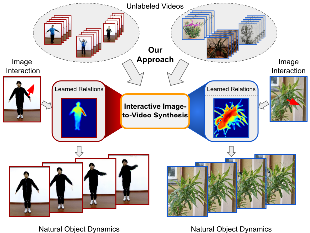
What would be the effect of locally poking a static scene? We present an approach that learns naturally-looking global articulations caused by a local manipulation at a pixel level. Training requires only videos of moving objects but no information of the underlying manipulation of the physical scene. Our generative model learns to infer natural object dynamics as a response to user interaction and learns about the interrelations between different object body regions. Given a static image of an object and a local poking of a pixel, the approach then predicts how the object would deform over time. In contrast to existing work on video prediction, we do not synthesize arbitrary realistic videos but enable local interactive control of the deformation. Our model is not restricted to particular object categories and can transfer dynamics onto novel unseen object instances. Extensive experiments on diverse objects demonstrate the effectiveness of our approach compared to common video prediction frameworks. Project page is available at https://bit.ly/3cxfA2L.

1 Introduction

From infancy on we learn about the world by manipulating our immediate environment and subsequently observing the resulting diverse reactions to our interaction. Particularly in early years, poking, pulling, and pushing the objects around us is our main source for learning about their integral parts, their interplay, articulation and dynamics. Consider children playing with a plant. They eventually comprehend how subtle touches only affect individual leaves, while increasingly forceful interactions may affect larger and larger constituents, thus finally learning about the entirety of the dynamics related to various kinds of interactions. Moreover, they learn to generalize these dynamics across similar objects, thus becoming able to predict the reaction of a novel object to their manipulation.

Training artificial visual systems to gain a similar understanding of the distinct characteristics of object articulation and its distinct dynamics is a major line of computer vision research. In the realm of still images the interplay between object shape and appearance has been extensively studied, even allowing for controlled, global [56, 54, 28, 22, 21] and local [52, 89] manipulation. Existing work on object dynamics, however, so far is addressed by either extrapolations of observed object motion [83, 37, 16, 45, 83, 59, 8, 76] or only coarse control of predefined attributes such as explicit action labels [87] and imitation of previously observed holistic motion [1, 20, 3]. Directly controlling and, even further, interacting with objects on a local level however, so far, is a novel enterprise.

Figure 1: Our approach for interactive image-to-video synthesis learns to understand the relations between the distinct body parts of articulated objects from unlabeled video data, thus enabling synthesis of videos showing natural object dynamics as responses to local interactions.

Teaching visual systems to understand the complex dynamics of objects both arising by explicit manipulations of individual parts and to predict and analyze the behavior [17, 4, 5] of the remainder of the object is an exceptionally challenging task. Similarly to a child in the example above, such systems need to know about the natural interrelations of different parts of an object [88]. Moreover, they have to learn how these parts are related by their dynamics to plausibly synthesize temporal object articulation as a response to our interactions.

In this paper, we present a generative model for interactive image-to-video synthesis which learns such a fine-grained understanding of object dynamics and, thus, is able to synthesize video sequences that exhibit natural responses to local user interactions with images on pixel-level. Using intuitions from physics [70], we derive a hierarchical recurrent model dedicated to model complex, fine-grained object dynamics. Without making assumptions on objects we learn to interact with and no ground-truth interactions provided, we learn our model from video sequences only.

We evaluate our model on four video datasets comprising the highly-articulated object categories of humans and plants. Our experiments demonstrate the capabilities of our proposed approach to allow for fine-grained user interaction. Further, we prove the plausibility of our generated object dynamics by comparison to state-of-the-art video prediction methods in terms of visual and temporal quality. Figure 1 provides an overview over the capabilities of our model.

2 Related Work

Video Synthesis. Video Synthesis involves a wide range of tasks including video-to-video translation [81], image animation [84, 67, 68], frame interpolation [60, 86, 50, 2, 61], unconditional video generation [78, 71, 13, 58] and video prediction. Given a set of context frames, video prediction methods aim to predict realistic future frames either deterministically [83, 77, 75, 85] or stochastically [23, 16, 77, 45, 83, 65, 59, 8, 76, 43]. A substantial number of methods ground on image warping techniques [79, 51, 25], leading to high-quality short term predictions, while struggling with longer sequence lengths. To avoid such issues, many works use autoregressive models. Due to consistently increasing compute capabilities, recent methods aim to achieve this task via directly maximizing likelihood in the pixel space, using large scale architectures such as normalizing flows [42, 43] or pixel-level transformers [74, 82]. As such methods introduce excessive computational costs and are slow during inference, most existing methods rely on RNN-based methods, acting autoregressively in the pixel-space [55, 45, 53, 16, 77, 8] or on intermediate representation such as optical flow [47, 46, 63]. However, since they have no means for direct interactions with a depicted object, but instead rely on observing past frames, these methods model dynamics in a holistic manner. By modelling dynamics entirely in the latent space, more recent approaches take a step towards a deeper understanding of dynamics [59, 24, 18] and can be used to factorize content from dynamics [24], which are nonetheless modeled holistically. In contrast, our model has to infer plausible motion based on local interactions and, thus, understands dynamics in a more fine-grained way.
Controllable Synthesis of Object Dynamics. Since it requires to understand the interplay between their distinct parts, controlling the dynamics of articulated objects is a highly challenging task. Davis et al. [15] resort to modeling rigid objects as spring-mass systems and animate still image frames by evaluating the resulting motion equations. However, due to these restricting assumptions, their method is only applicable for small deviations around a rest state, thus unable model complex dynamics.

To reduce complexity, existing learning based approaches often focus on modelling human dynamics using low-dimensional, parametric representations such as keypoints [1, 87, 3], thus preventing universal applicability. Moreover, as these approaches are either based on explicit action labels or require motion sequences as input, they cannot be applied to controlling single body parts. When intending to similarly obtain control over object dynamics in the pixel domain, previous methods use ground truth annotations such as holistic motion trajectories [23, 45, 18] for simple object classes without articulation [19]. Hao et al. [31] step towards locally controlling the video generation process by predicting a single next images based on a given input frame and sets of sparse flow vectors. Their proposed approach, however, requires multiple flow vectors for each individual frame of a sequence to be predicted, thus preventing localized, fine-grained control. Avoiding such flaws and indeed allowing for localized control, our approach introduces a latent dynamics model, which is able to model complex, articulated motion based on an interaction at a single pixel.

Figure 2: Left: Our framework for interactive image-to-video synthesis during training. Right: Our proposed hierarchical latent model $\boldsymbol{\mathcal{F}}$ for synthesizing dynamics, consisting of a hierarchy of individual RNNs $\mathcal{F}_{n}$, each of which operates on a different spatial feature level of the UNet defined by the pretrained encoder $\mathcal{E}_{\sigma}$ and the decoder $\mathcal{G}$. Given the initial object state $\boldsymbol{\sigma}_{0}=[\mathcal{E}_{\sigma}(x_{0})^{1},...,\mathcal{E}_{\sigma}(x_{0})^{N}]$, $\boldsymbol{\mathcal{F}}$ predicts the next state $\boldsymbol{\hat{\sigma}}_{i+1}=[\hat{\sigma}_{i+1}^{1},...,\hat{\sigma}_{i+1}^{N}]$ based on its current state $\hat{\sigma}_{i}$ and the latent interaction $\phi_{i}=\mathcal{E}_{\phi}(p,l)$ at the corresponding time step. The decoder $\mathcal{G}$ finally visualizes each predicted object state $\hat{\sigma}_{i}$ in an image frame $\hat{x}_{i}$.

3 Interactive Image-to-Video Synthesis

Given an image frame $x_{0}\in\mathbb{R}^{H\times W\times 3}$, our goal is to interact with the depicted objects therein, i.e. we want to initiate a poke $p\in\mathbb{R}^{2}$ which represents a shift of a single location $l\in\mathbb{N}^{2}$ within $x_{0}$ to its new target location. Moreover, such pokes should also influence the remainder of the image in a natural, physically plausible way.

Inferring the implications of local interactions upon the entire object requires a detailed understanding of its articulation, and, thus, of the interrelation between its various parts. Consequently, we require a structured and concise representation of the image $x_{0}$ and a given interaction. To this end, we introduce two encoding functions: an object encoder $\mathcal{E}_{\sigma}$ mapping images $x$ onto a latent object state $\sigma=\mathcal{E}_{\sigma}(x)$, e.g. describing current object pose and appearance, and the encoder $\mathcal{E}_{\phi}$ translating the target location defined by $p$ and $l$ to a latent interaction $\phi=\mathcal{E}_{\phi}(p,l)$ now affecting the initially observed object state $\sigma_{0}=\mathcal{E}_{\sigma}(x_{0})$.

Eventually, we want to synthesize a video sequence depicting the response arising from our interaction with the image $x_{0}$, represented by means of $\sigma_{0}$ and $\phi$. Commonly, such conditional video generation tasks are formulated by means of learning a video generator $\mathcal{G}:(\sigma_{0},\phi)\rightarrow X_{1:T}=\{x_{1},...,x_{T}\}$ [45, 8]. Thus, $\mathcal{G}$ would both model object dynamics and infer their visualization in the RGB space. However, every object class has its distinct, potentially very complex dynamics which - affecting the entire object - must be inferred from a localized poke shifting a single pixel. Consequently, a model for interactive image-to-video synthesis has to understand the complex implications of the poke for the remaining object parts and, thus, requires to model these dynamics in sufficiently fine-grained and flexible way. Therefore, we introduce a dedicated object dynamics model inferring a trajectory of object states $[\sigma_{0},\sigma_{1},\dots,\sigma_{T}]$ representing an object’s response to $\phi$ within an object state space $\Omega$. As a result, $\mathcal{G}$ only needs to generate the individual images $x_{i}=\mathcal{G}(\sigma_{i})$, thus decomposing the overall image-to-video synthesis problem.

Figure 3: Visualization of the videos generated by our model for two distinct plants within our self-recorded PokingPlants-Dataset: The first row depicts a ground truth sequence from the test set. The second row contains a simulated poke (red arrow) based on this ground truth sequence, using the procedure described in Section 3.2. The last two rows show results of the model to pokes from human users. In the first column, the red arrow indicates the interaction and, thus, also the resulting target location, which is indicated as a red dot in the remaining columns. As the motions within the Poking-Plants dataset are sometimes subtle and not straightforward to detect, we also visualize the visual flow field, which was estimated based on the synthesized videos. We encourage the reader to also view the corresponding video results in the supplemental and on our project page https://bit.ly/3cxfA2L.

3.1 A Hierarchical Model for Object Dynamics

In physics, one would typically model the trajectory of object states $\sigma(t)$ as a dynamical system and, thus, describe it as an ordinary differential equation (ODE) [70, 9]

$$\dot{\sigma}(t)=f(\sigma(t),\phi(t))\,,\,\sigma(0)=\sigma_{0}\,,$$ (1)

with $f$ the - in our case unknown - evolution function, $\dot{\sigma}$ its first time derivative, and $\phi(t)=\phi~{},~{}\forall t\in[0,T]$ the latent external interaction obtained from the poke. Recent work proposes to describe $f$ with fixed model assumptions, such as as an oscillatory system [15]. While this may hold in some cases, it greatly restricts applications to arbitrary, highly-articulated object categories. Avoiding such strong assumptions, the only viable solution is to learn a flexible prediction function $\mathcal{F}$ representing the dynamics in Eq. (1). Consequently, we base $\mathcal{F}$ on recurrent neural network models [33, 11] which can be interpreted as a discrete, first-order approximation to Eq. (1) at time steps $i\in[0,T-1]$

$$\mathcal{F}(\sigma_{i},\phi_{i})=\sigma_{i+1}=\sigma_{i}+h\cdot f_{a}(\sigma_{i},\phi_{i})\,,$$ (2)

with $h$ being the step size between two consecutive predicted states $\sigma_{i}$ and $\sigma_{i+1}$ and $f_{a}$ an approximation to the derivative at $\sigma_{i}$ [9, 62]. However, dynamics of objects can be arbitrarily complex and subtle such as leaves of a tree or plant fluttering in the wind. In such cases, the underlying evolution function $f$ is expected to be similarly complex and, thus, involving only first-order derivatives when modelling Eq. (1) may not be sufficient. Instead, capturing also such high-frequency details actually calls for higher-order terms.

In fact, one can model an $N$-th order evolution function in terms of $N$ first order ODEs, by introducing a hierarchy $\boldsymbol{\sigma}=[\sigma^{1},...,\sigma^{N}]\,,\,\sigma^{1}=\sigma$ of state variables, the $n$-th element of which is proportional to the $(n-1)$-th order of discrete time derivative of the original variable $\sigma$ [30, 62]. Consequently, as first order ODEs can be well approximated with Eq. (2), we can extend $\mathcal{F}$ to a hierarchy of predictors $\boldsymbol{\sigma}=\boldsymbol{\mathcal{F}}=[\mathcal{F}_{1},...,\mathcal{F}_{N}]$ by using a sequence of $N$ RNNs,

$$\sigma^{n}_{i+1}=\mathcal{F}_{n}(\sigma_{i}^{n},\sigma_{i+1}^{n-1})\,,\sigma^{n}_{0}=\sigma_{0}$$ (3)

each operating on the input of its predecessor, except for the lowest level $\mathcal{F}_{1}$, which predicts the coarsest approximation of the object states based on $\phi_{i}$ as

$${\sigma}^{1}_{i+1}=\mathcal{F}_{1}(\sigma^{1}_{i},\phi_{i})\,,\,\sigma^{1}_{0}=\sigma_{0}\,.$$ (4)

A derivation of our this hierarchy is given in the Appendix C. However, while $\boldsymbol{\mathcal{F}}$ is able to approximate higher-order derivatives up to order $N$, thus being able to model fine-grained dynamics, we need to make sure that our decoder $\mathcal{G}$ actually captures these details when generating the individual image frames $x_{i}$.

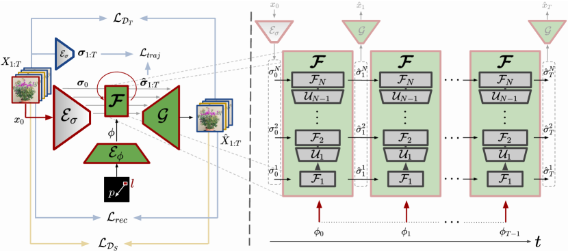
Recent work on image synthesis indicates that standard decoder architectures fed with latent encodings only on the bottleneck-level, are prone to missing out on subtle image details [39, 64], such as those arising from high motion frequencies. Instead, providing a decoder with latent information at each spatial scale has proven to be more powerful [66]. Hence, we model $\mathcal{G}$ to be the decoder of a hierarchical image-to-sequence UNet with the individual predictors $\mathcal{F}_{n}$ operating on the different spatial feature levels of $\mathcal{G}$. To maintain the hierarchical structure of $\boldsymbol{\mathcal{F}}$, we compensate for the resulting mismatch between the dimensionality of $\sigma_{i}^{n-1}$ and $\sigma_{i}^{n}$ by means of upsampling functions $\mathcal{U}_{n}$. Finally, to fully exploit the power of a UNet structure, we similarly model the encoder $\mathcal{E}_{\sigma}$ to yield a hierarchical object state $\boldsymbol{\sigma}_{0}=[\mathcal{E}_{\sigma}(x_{0})^{1},...,\mathcal{E}_{\sigma}(x_{0})^{N}]$, which is the initial state to $\boldsymbol{\mathcal{F}}$. Thus, Eq. (3) becomes

$$\sigma^{n}_{i+1}=\mathcal{F}_{n}(\sigma_{i}^{n},\mathcal{U}_{n-1}(\sigma_{i+1}^{n-1}))\,,\sigma^{n}_{0}=\mathcal{E}_{\sigma}(x_{0})^{n}$$ (5)

with $\sigma^{n}_{i}$ being the predicted object state at feature level $n\in[2,N]$ and time step $i$. Hence, at each time step we obtain a hierarchy of $N$ latent object states $\boldsymbol{\sigma}_{i}=[\sigma^{1}_{i},...,\sigma^{N}_{i}]$ on different spatial scales, which are the basis for synthesizing image frames $x_{i}$ by $\mathcal{G}$. Our full hierarchical predictor $\boldsymbol{\mathcal{F}}$ and its linkage to the overall architecture are shown in the right and left parts of Figure 2.

As our proposed model jointly adds more subtle details in the temporal and spatial domain, it accurately captures complex dynamics arising from interactions and simultaneously displays them in the image space.

Figure 4: Visualization of the videos generated by our model for two actors within the test set of the iPER [49] dataset: The first row depicts the ground truth sequence. The second row contains a simulated poke (red arrow) based on this ground truth sequence, using the procedure described in Section 3.2. The last two rows show results of the model to pokes from human users. In the first column, the red arrow indicates the interaction and, thus, also the resulting target location, which is indicated as a red dot in the remaining columns. We encourage the reader to also view the accompanying video results in the supplemental and on our project page https://bit.ly/3cxfA2L.

3.2 Learning Dynamics from Poking

To learn our proposed model for interactive image-to-video synthesis, we would ideally have ground-truth interactions provided, i.e. actual pokes and videos of their immediate impact on the depicted object in $x_{0}$. However, gathering such training interactions is tedious and in some cases not possible at all, particularly hindering universal applicability. Consequently, we are limited to cheaply available video sequences and need to infer the supervision for interactions automatically.

While at inference a poke $p$ represents an intentional shift of an image pixel in $x_{0}$ at location $l$, at training we only require to observe responses of an object to some shifts, as long as the inference task is well and naturally approximated. To this end, we make use of dense optical flow displacement maps [34] $D\in\mathbb{R}^{H\times W\times 2}$ between images $x_{0}$ and $x_{T}$ of our training videos, i.e. their initial and last frames. Simulating training pokes in $x_{0}$ then corresponds to sampling pixel displacements $p=(D_{l_{1},l_{2},1},D_{l_{1},l_{2},2})$ from $D$, with the video sequence $X_{1:T}=\{x_{i}\}_{i=1}^{T}$ being a natural response to $p$. Using this, we train our interaction conditioned generative model to minimize the mismatch between the individual predicted image frames $\hat{x}_{i}=\mathcal{G}(\boldsymbol{\mathcal{F}}(\boldsymbol{\sigma}_{i-1},\phi_{i-1}))$ and those of the video sequence as measured by the perceptual distance [38]

$$\mathcal{L}_{rec}=\sum_{i=1}^{T}\sum_{k=1}^{K}\|\Phi_{k}(x_{i})-\Phi_{k}(\hat{x}_{i})\|_{1}\,,$$ (6)

where $\Phi_{k}$ denotes the $k$-th layer of a pre-trained VGG [69] feature extractor.

However, due to the direct dependence of $\mathcal{G}$ on $\boldsymbol{\sigma}_{i}$, during end-to-end training the state space $\Omega$ is continuously changing. Thus, learning object dynamics by means of our hierarchical predictor $\boldsymbol{\mathcal{F}}$ is aggravated. To alleviate this issue, we propose to first learn a fixed object space state $\Omega$ by pretraining $\mathcal{E}_{\sigma}$ and $\mathcal{G}$ to reconstruct individual image frames. Training $\boldsymbol{\mathcal{F}}$ on $\Omega$ to capture dynamics depicted in $\{x_{i}\}_{i=0}^{T}$ is then performed by predicting states $\boldsymbol{\hat{\sigma}}_{i}=\boldsymbol{\mathcal{F}}(\boldsymbol{\hat{\sigma}}_{i-1},\phi_{i})$ approaching the individual states $\boldsymbol{\sigma}_{i}=[\mathcal{E}_{\sigma}(x_{i})^{1},...,\mathcal{E}_{\sigma}(x_{i})^{N}]$ of the target trajectory, while simultaneously fine-tuning $\mathcal{G}$ to compensate for prediction inaccuracy, using

$$\mathcal{L}_{traj}=\sum_{i=1}^{T}\sum_{n=1}^{N}\|\mathcal{E}_{\sigma}(x_{i})^{n}-\hat{\sigma}^{n}_{i}\|_{2}\,.$$ (7)

Finally, to improve the synthesis quality we follow previous work [13, 81] by training discriminators $\mathcal{D}_{S}$ on frame level and $\mathcal{D}_{T}$ on the temporal level, resulting in loss functions $\mathcal{L}_{\mathcal{D}_{S}}$ and $\mathcal{L}_{\mathcal{D}_{T}}$. Our overall optimization objective then reads

$$\mathcal{L}=\mathcal{L}_{rec}+\lambda_{traj}\cdot\mathcal{L}_{traj}+\lambda_{S}\cdot\mathcal{L}_{\mathcal{D}_{S}}\,+\lambda_{\mathcal{D}_{T}}\cdot\mathcal{L}_{D_{T}}$$ (8)

with hyperparameters $\lambda_{traj}$, $\lambda_{S}$ and $\lambda_{T}$. The overall procedure for learning our network is summarized in Fig. 2.

Figure 5: Understanding object structure: By performing 100 random interactions at the same location $l$ within a given image frame $x_{0}$ we obtain varying video sequences, from which we compute motion correlations for $l$ with all remaining pixels. By mapping these correlations to the pixel space, we visualize distinct object parts. For a detailed discussion, refer to Section 4.2.

4 Experiments

In this section we both qualitatively and quantitatively analyze our model for the task of interactive image-to-video synthesis. After providing implementation details, we illustrate qualitative results and analyze the learned object interrelations. Finally, we conduct a quantitative evaluation of both visual quality of our generated videos and the plausibility of the motion dynamics depicted within.

4.1 Implementation Details and Datasets

Foreground-Background-Separation. While our model should learn to capture dynamics associated with objects initiated by interaction, interaction with areas corresponding to the background should be ignored. However, optical flow maps often exhibit spurious motion estimates in background areas, which may distort our model when considered as simulated object pokes for training. To suppress these cases we only consider flow vector exhibiting sufficient motion magnitude as valid pokes, while additionally training our model to ignore background pokes. More details are provided in Appendix E.2. Examples for responses to background interactions can be found in the videos on our project page https://bit.ly/3cxfA2L.
Model Architecture and Training. The individual units $\mathcal{F}_{n}$ of our hierarchical dynamics model are implemented as Gated Recurrent Units (GRU) [11]. The depth $N$ of our hierarchy of predictors varies among datasets and videos resolutions. For the experiments shown in the main paper, we train our model to generate sequences of 10 frames and spatial size $128\times 128$, if not specified otherwise. For training, we use ADAM [41] optimizer with parameters $\beta=(0.9,0.99)$ and a learning rate of $10^{-4}$. The batch size during training is 10. The weighting factors for our final loss function are chosen as $\lambda_{traj}=0.1$, $\lambda_{\mathcal{D}_{S}}=0.2$ and $\lambda_{\mathcal{D}_{T}}=1$. More details regarding architecture, hyperparameters and training can be found in the Appendix E. Additionally, alternate training procedures for different parameterizations of the poke and the latent interaction $\phi(t)$ are presented in Appendix B.
Datasets We evaluate the capabilities of our model to understand object dynamics on four datasets, comprising the highly-articulated object categories of humans and plants.

Poking-Plants (PP) is a self-recorded dataset showing 27 video sequences of 13 different types of pot plants in motion. As the plants within the dataset have large variances in shape and texture, it is particularly challenging to learn a single dynamics model from those data. The dataset consists of overall 43k image frames, of which we use a fifth as test and the remainder as train data.

iPER [49] is a human motion dataset containing 206 video sequences of 30 human actors of varying shape, height gender and clothing, each of which is recorded in 2 videos showing simple and complex movements. We follow the predefined train test split with a train set containing 180k frames and a test set consisting of 49k frames.

Tai-Chi-HD [68] is a video collection of 280 in-the-wild Tai-Chi videos of spatial size $256\times 256$ from youtube which are subdivided into 252 train and 28 test videos, consisting of 211k and 54k image frames. It contains large variances in background and also camera movements, thus serving as an indicator for the real-world applicability of our model. As the motion between subsequent frame is often small, we temporally downsample the dataset by a factor of two.

Human3.6m [35] is large scale human motion dataset, containing video sequences of 7 human actors performing 17 distinct actions. Following previous work on video prediction [83, 59, 24], we centercrop and downsample the videos to 6.25 Hz and use actors S1,S5,S6,S7 and S8 for training and actors S9 and S11 for testing.

4.2 Qualitative Analysis

Dataset	PP	iPER	Tai-Chi	H3.6m
SAVP [45]	136.81	150.39	309.62	160.32
IVRNN [8]	184.54	181.50	202.33	465.55
SRVP [24]	283.90	245.13	238.71	174.65
Ours	89.67	144.92	171.74	107.73

Table 1: Comparison with recent work from video prediction. Across datasets, our approach obtains considerably lower FVD-scores.

Dataset	PP		iPER [49]		TaiChi [68]		Human3.6m [35]
Method	Ours	Hao et al. [31]	Ours	Hao et al. [31]	Ours	Hao et al. [31]	Ours	Hao et al. [31]
FVD $\downarrow$	137.78	361.51	93.28	235.08	152.76	341.79	100.36	259.92
LPIPS $\downarrow$	0.10	0.16	0.06	0.11	0.12	0.12	0.08	0.10
PSNR $\uparrow$	20.68	21.28	23.99	21.09	20.58	20.41	23.71	22.81
SSIM $\uparrow$	0.78	0.72	0.91	0.88	0.75	0.78	0.92	0.93

Table 2: Comparison on controlled video synthesis. We compare with Hao et al. [31] which we consider the closest previous work to ours.

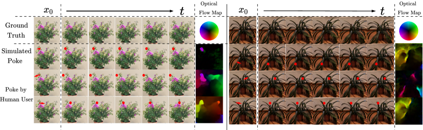
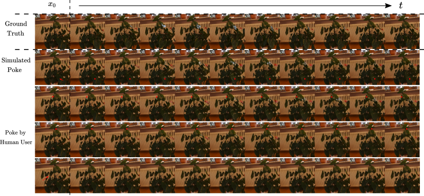
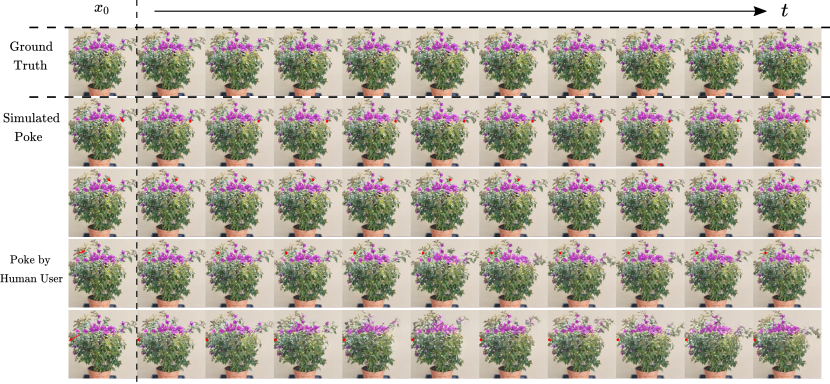
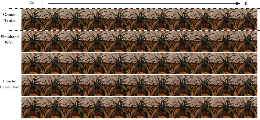
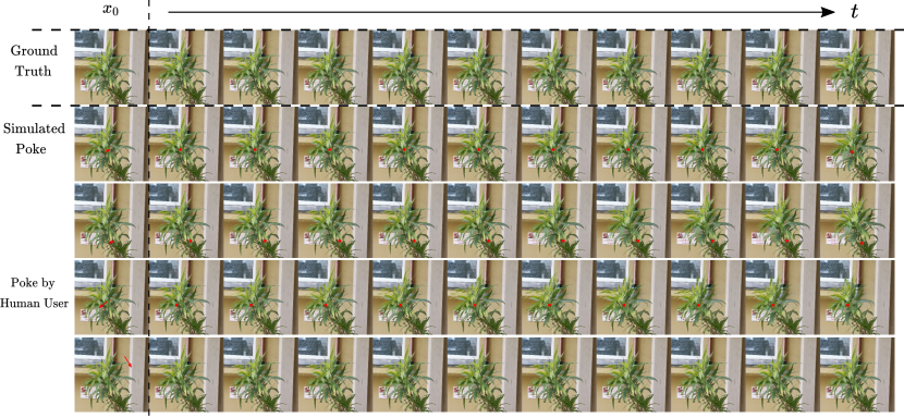
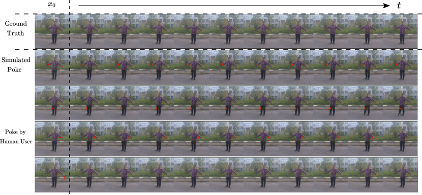
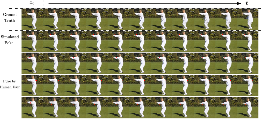
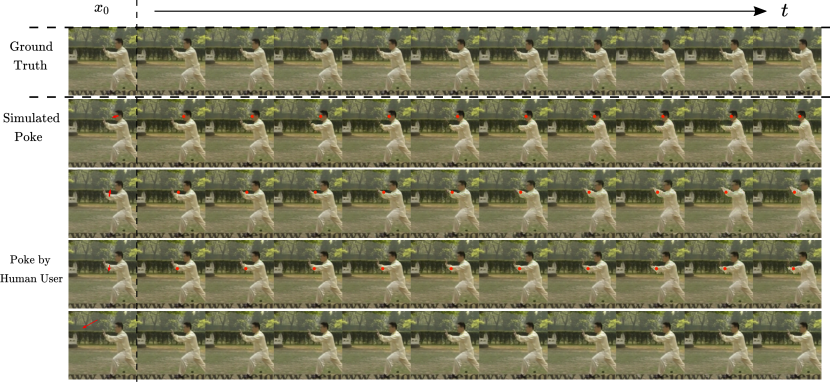
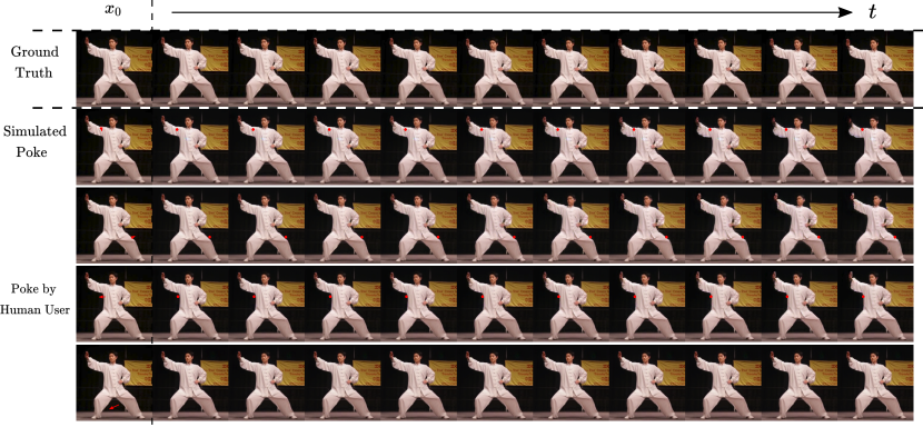
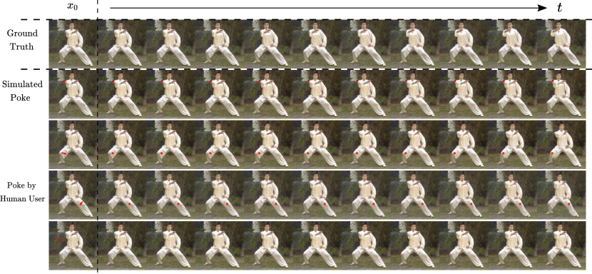
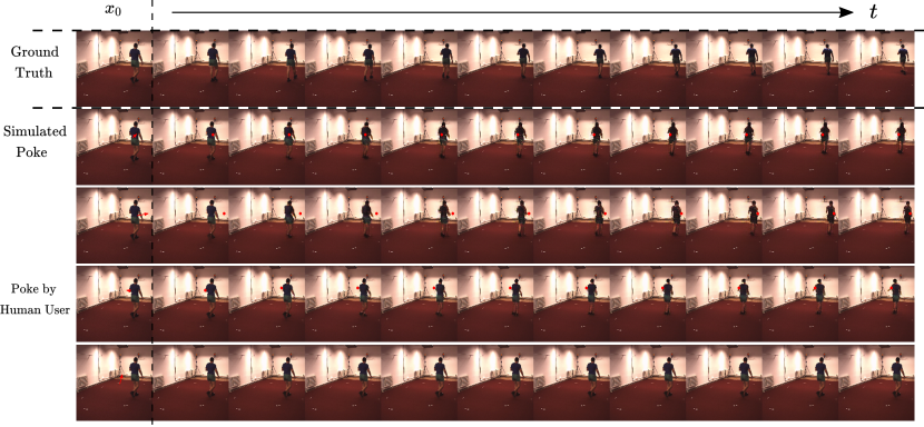
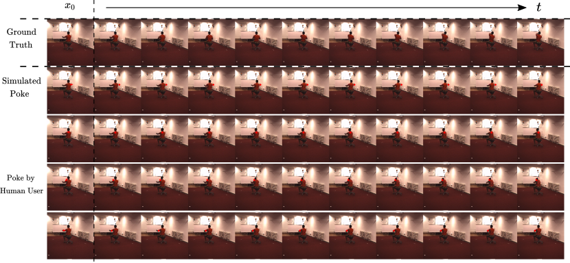
Interactive Image-to-Video-Synthesis. We now demonstrate the capabilities of our model for the task of interactive image-to-video synthesis. By poking a pixel within a source image $x_{0}$, i.e. defining the shift $p$ between the source location $l$ and the desired target location, we require our model to synthesize a video sequence showing the object part around $l$ approaching the defined target location. Moreover, the model should also infer plausible dynamics for the remaining object parts. Given $x_{0}$, we visualize the video sequences generated by our model for $i)$ simulated pokes obtained from optical flow estimates (see Sec. 3.2) from test videos and $ii)$ pokes initiated by human users. We compare them to the corresponding ground truth videos starting with $x_{0}$. For the object category of plants, we also show optical flow maps between the source frame and the last frame for each generated video, to visualize the overall motion therein.

Figure 3 shows examples for two distinct plants from the PokingPlants dataset of very different appearance and shape. In the left example we interact with the same pixel location varying both poke directions and magnitudes. Our model correctly infers corresponding object dynamics. Note that the interaction location corresponds to a very small part of the plant, initiating both subtle and complex motions. This demonstrates the benefit of our hierarchical dynamics model. As shown by the visualized flow, the model also infers plausible movements for object parts not directly related to the interaction, thus indicating our model to also understand long term relations between distinct object regions. In the right example we observe similar results when interacting with different locations.

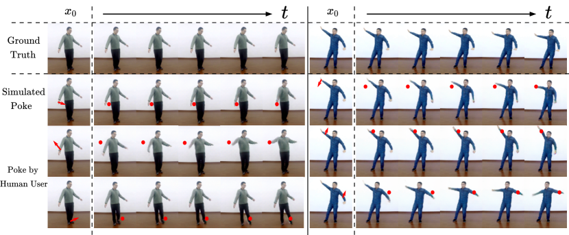
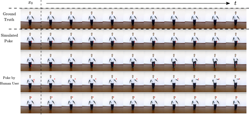
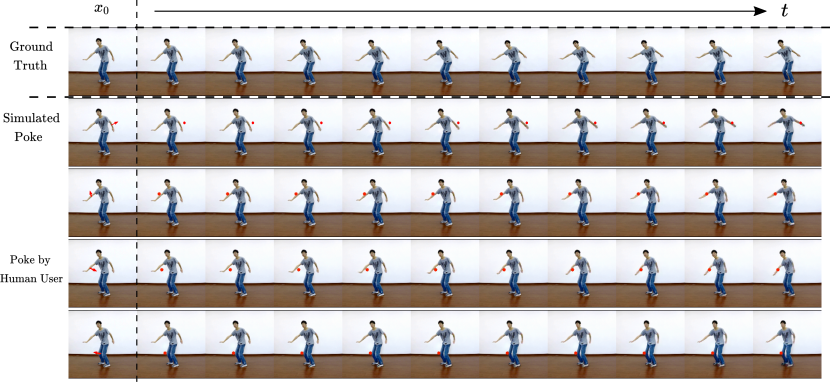
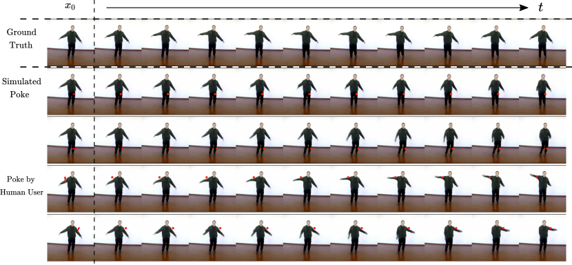
As our model does not make any assumptions on the depicted object to manipulate, we are not restricted to particular object classes. To this end we also consider the category of humans which is widely considered for various video synthesis tasks. Figure 4 shows results for two unseen persons from the iPER test set. Again our model infers natural object dynamics for both the interaction target location and the entire object. This highlights that our model is also able to understand highly structured dynamics and natural interrelations of object parts independent of object appearance. Analogous results for the Tai-Chi-HD and Human3.6m datasets are contained in the Appendix A.
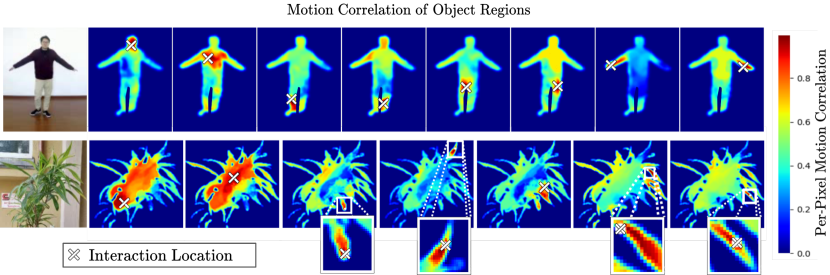
Understanding Object Structure. We now analyze the interrelation of object parts learned by our model, i.e. how pixels depicting such parts correlate when interacting with a specific, fixed interaction location.

To this end, we perform $100$ random interactions for a given, fixed source frame $x_{0}$ at the fixed location $l=(l_{1},l_{2})$ of different magnitudes and directions. This results in varying videos $\{\hat{X}_{k}\}_{k=1}^{100}$, exhibiting distinct dynamics of the depicted object. To measure the correlation in motion of all pixels with respect to the interaction location, we first obtain their individual motion for each generated video using optical flow maps between $x_{0}$ and the last video frames. Next, for each pixel we compute the L2-distance in each video to the respective interaction poke based on a $[\text{magnitude},\text{angle}]$ representation, thus obtaining a $100$-dimensional difference vector. To measure the correlation for each pixel with $l$, we now compute the variance over each difference vector to obtain correlation maps. High correlation then corresponds to low variance in motion.

Figure 5 visualizes such correlations by using heatmaps for different interaction locations $l$ in the same source frame $x_{0}$ for both plants and humans. For humans, we obtain high correlations for the body parts around $l$, indicating our model to actually understand the human body structure. Considering the plant, we see that poking locations on its trunk (first two columns) intuitively results in highly similar movements of all those pixels close to the trunk. The individual leaves farther away are not that closely correlated, as they might perform oscillations in higher frequencies superposing the generally low-frequency movements of the trunk. When poking these leaves, however, mostly directly neighbouring pixels exhibit high correlation.

4.3 Quantitative Evaluation

To quantitatively demonstrate the ability of our approach to synthesize plausible object motion, we compare with the current state-of-the-art of RNN-based video prediction [45, 8, 24]. For all competing methods we used the provided pretrained models, where available, or trained the models using official code. Moreover, to also evaluate the controllable aspect of our approach, we compare against Hao et al. [31], an approach for controlled video synthesis by predicting independent single frames from sparse sets of flow vectors, which we consider the closest previous work to interactive image-to-video synthesis. We trained their method on our considered datasets using their provided code.
Evaluation Metrics. For evaluation we utilize the following metrics. Additional details on all metrics are listed in Appendix F.

Motion Consistency. The Fréchet-Video-Distance (FVD, lower-is-better) is the standard metric to evaluate video predictions tasks, as it is sensitive to the visual quality, as well as plausibility and consistency of motion dynamics of a synthesized video. Moreover it has been shown to correlate well with human judgement [73]. All FVD-scores reported hereafter are obtained from video sequences of length 10.

Prediction accuracy. Our model is trained to understand the global impact of localized pokes on the overall object dynamics and to infer the resulting temporal object articulation. To evaluate this ability, we report distance scores against the ground-truth using three commonly used frame-wise metrics, averaged over time: SSIM (higher-is-better) and PSNR (higher-is-better) directly compare the predicted and ground truth frames. Since they are based on L2-distances directly in pixel space, they are known disregard high-frequency image details, thus preferring blurry predictions. To compensate, we also report the LPIPS-score [90] (lower-is-better), comparing images based on distance between activations of pretrained deep neural network and, thus exhibit better correlation with human judgment.
Comparison to other methods. We evaluate our approach against SAVP [45], IVRNN [8] and SRVP [24] which are RNN-based state-of-the-art methods in video prediction based on FVD scores. We train these models to predict video sequences of length 10 given 2 context frames corresponding to the evaluation setting. Note, that our method generates sequences consisting of 10 frames based on a single frame and a poke. Following common evaluation practice in video prediction [45, 8, 24], we predict sequences are $64\times 64$ for all models, including ours. The results are shown in Tab. 1. Across datasets, our approach achieves significantly lower FVD-scores demonstrating the effectiveness of our approach to both infer and visualize plausible object dynamics. Particularly on the plants dataset our model performs significantly better than the competitors due to our proposed hierarchic model for capturing fine-grained dynamics.

To quantitatively evaluate our ability for controlled video synthesis, we now compare against Hao et al. [31]. For them to predict videos $[x_{0},\dots,x_{T}]$ of length $T$, we first sample $k$ flow vectors between $x_{0}$ and $x_{1}$. We then extend these initial vectors to discrete trajectories of length $T-1$ in the image space by tracking the initial points using consecutive flow vectors between $x_{i}$ and $x_{i+1}$. Video prediction is then performed by individually warping $x_{0}$ given the shift of its pixels to the intermediate locations at step $i$ in these trajectories. Following their protocol we set $k=5$. Note, that we only require a single interactive poke of arbitrary length for synthesize videos. Tab. 2 compares both approaches. We see that our model performs significantly better by a large margin, especially in FVD measuring the video quality and temporal consistency. This is explained by temporal object dynamics not even being considered in [31], in contrast to our dedicated hierarchical dynamics model. Further, their image warping-based approach typically results in blurry image predictions. Across datasets we outperform their method also in LPIPS scores indicating our proposed method to produce more visually compelling results.

4.4 Ablation Studies

Finally, we conduct ablation studies to analyze the effects of the individual components of our proposed method. To limit computational cost, we conduct all ablation experiments using videos of spatial size $64\times 64$. Ours RNN indicates our model trained with a common GRU consisting of three individual cells at the latent bottleneck of the UNet instead of our proposed hierarchy of predictors $\boldsymbol{\mathcal{F}}$. For fair evaluation with the baselines we also choose $N=3$ as depth of the hierarchy. Further, we also evaluate baselines without considering the loss term $\mathcal{L}_{traj}$ which compensates for the prediction inaccuracy of $\boldsymbol{\mathcal{F}}$ (Ours w/o $\mathcal{L}_{traj}$) and without pretraining the object encoder $\mathcal{E}_{\sigma}$ (Ours single-stage). Tab. 3 summarizes the ablation results, indicating the the benefits of each individual component across reported metrics and used datasets. We observe the largest impact when using our hierarchical predictor $\boldsymbol{\mathcal{F}}$, thus modelling higher-order terms in our dynamics model across all spatial feature scales. Looking at the remaining two ablations, we also see improvements in FVD-scores. This concludes that operating on a pretrained, consistent object state space $\Omega$ and subsequently accounting for the prediction inaccuracies, leads to significantly more stable learning. An additional ablation study on the effects of varying the highest order $N$ of modeled derivative by our method is provided in Appendix D.

4.5 Additional Experiments

We also conduct various alternate experiments, including the generalization of our model to unseen types of plants and different interpretations of the poke $p$, resulting in different capabilities of our model. These experiments are contained in the Appendix B, which also contains many videos further visualizing the corresponding results.

5 Conclusion

In this work, we propose a generative model for interactive image-to-video synthesis which learns to understand the dynamics of articulated objects by capturing the interplay between the distinct object parts, thus allowing to synthesize videos showing natural responses to localized user interactions. The model can be flexibly learned from unlabeled video data without limiting assumptions on object shape. Experiments on a range of datasets prove the plausibility of generated dynamics and indicate the model to produce visually compelling video sequences.

Dataset	PP			iPER [49]
Method	LPIPS $\downarrow$	PSNR $\uparrow$	FVD $\downarrow$	LPIPS $\downarrow$	PSNR $\uparrow$	FVD $\downarrow$
Ours RNN	0.08	20.92	175.42	0.07	23.02	250.64
Ours w/o $\mathcal{L}_{traj}$	0.07	21.53	110.00	0.05	22.82	203.26
Ours (single)	0.07	21.41	115.65	0.06	23.09	220.82
Ours full	0.06	21.81	89.67	0.05	23.49	144.92

Table 3: Ablation studies on the PokingPlants and iPER datasets

Preliminaries

For all of our reported datasets in the main paper, we provide additional video material resulting in 24 videos in total. For each video three individual cycles are shown (indicated left bottom) as well as the corresponding frame-per-second (FPS) rate (right bottom). Analogous to the main paper, the direction of the poke is indicated by a red arrow starting at the poke location $l$ and the target location is marked by a red dot, if not stated otherwise. The file structure of the videos is as follows:

  supplementary_material_244
        |
        +--A-Additional_Visualizations
            |
            +--A1-PokingPlants
            |
            +--A2-iPER
            |
            +--A3-Tai-Chi-HD
            |
            +--A4-Human36M
            |
            +--A5-Qualitative_Comparison
            |
        +--B-Additional_Experiments
            |
            +--B2-Impulse_Model
            |
            +--B3-Generalization

In Section A, we discuss our qualitative results and further emphasize the effectiveness of our approach by visually comparing with two competitors from the main paper. In Section B we acquire two additional experiments which are based on a slightly different training procedure and a different interpretation of the poke: first, we introduce the training procedure. We then visually evaluate the trained model and subsequently show this model to generalize to previously unseen types of plants which are obtained using web-search. After discussing the results, we derive Equation (3) from the main paper within Section C. Moreover, to provide empirical evidence for the effects of selecting the highest order of ODE derivative modeled by our method, we show the benefits of increasing the depth of the RNN hierarchy corresponding to an increase in this order in an additional ablation study in Section D. In conclusion we describe implementation and evaluation details in the Sections E and  F.

Appendix A Additional Visualizations

Subsequently, we discuss our obtained results for each dataset individually, before visually comparing our approach with two competing methods from the quantitative evaluation section. Within the section-specific directory ’...--A-Additional_Visualizations’, each subsection matches its corresponding folder (e.g. ’A.1.PokingPlants’ corresponds to ’...--A1-PokingPlants’) containing the discussed video sequences. Each video file compares synthesized sequences of our model for a simulated poke and three pokes initiated by human users with the ground truth sequence starting with the same initial image $x_{0}$, except for those videos containing the comparisons to the related methods.

A.1 PokingPlants

We provide four videos (poking_plants_[1-4].mp4) for the PokingPlants dataset showing distinct types of plants of substantially different shapes and appearances. Despite these large variances, our model generates realistic and appealing visualizations which are plausible responses to the poke. Pokes of large magnitudes (indicated by longer arrows) result in larger object motion, affecting not only the object parts in the vicinity of the poke location, but also those parts farther away. This illustrates that our model captures long-term relations between distinct object regions. Modest interactions, in contrast, result in much finer object motions. For instance, the subtle poke initiated in the third column of poking_plants_2.mp4 only results in fine-grained movements of those parts next to the poke location, whereas the large interaction in the last column causes nearly the entire plant to heavily oscillate. In summary, the examples demonstrate the capabilities of our method to flexibly model dynamics even for object categories with large intra-class variance, ranging from large scale low frequency motion to very subtle movements. Moreover, our model consistently accomplishes to generate sequences showing the object regions around the poke location to approach the target location. We also provide examples for background interactions in the last columns of the examples poking_plants_1.mp4 and poking_plants_4.mp4 which indicate our model to separate those pixels comprising the object from background clutter. Note, that we also plot the individual image frames of the generated videos in Figures 6-9 together with the target locations and the pokes.

A.2 iPER

For the iPER [49] dataset, we also provide four videos (iper_[1-4].mp4) containing unseen actors in indoor as well as outdoor scenes. When comparing the synthesized motion, which is generated based on simulated pokes (second columns), with the ground truth sequences depicted in the first columns, one can clearly observe, that our proposed method achieves to infer realistic global motion only from those sparse, localized interactions. The model can even generate complex human dynamics including distinct combinations of the arms and legs resulting from large pokes, as visualized in the third column of iper_1.mp4. Furthermore, it generalizes well to out-of-distribution settings as indicated by the example iper_4.mp4 showing an actor in the wild  and is capable to separate background from foreground also in such cases. Similar to the PokingPlants dataset, we visualize the individual image frames of the generated sequences together with the pokes and target locations in Figures 10-13.

A.3 Tai-Chi-HD

We now visualize examples for the Tai-Chi-HD [68] dataset, which does not contain movements as large as those in iPER, but is nonetheless challenging, since it contains many in-the-wild scenes with highly textured background and substantial amounts of camera movements. Thus, we use it to demonstrate our method to be also able to handle such real-world conditions. As for the other datasets discussed so far, we prepared four videos (taichi_[1-4].mp4; the individual image frames are shown in Figures 14-17). Also for this dataset, the model infers plausible global motions from the poke as indicated by the examples obtained from the simulated poke, which are similar to the ground truth sequences for all provided visualizations. Moreover, the model generates plausible responses to user interactions, demonstrating our model to be applicable to outdoor conditions. This is further emphasized by the capability of our model to separate the object area from the background in the presence of camera movements and background clutter.

A.4 Human3.6M

Finally, we show exemplary results of our method on the Human3.6m [35] dataset, which is challenging due to the complexity of performed motions and the low number of different unique persons. Consequently during testing, appearance swaps after a small number of predicted frames are frequently observed [83, 59, 24]. As the majority of actions performed by the persons are either based on walking or sitting we visualize examples for both these cases (h36m_[1,2].mp4; corresponding image enrollmentin Figure 18+19). In the first example, we use the poke to control the walking direction of the depicted actor as well as the covered distance. Although changing the appearance, our model generates plausible dynamics which are responses to the individual pokes. In the second example, we interact with the depicted person by manipulating its torso, head and arms. In summary, the visualizations demonstrate that our model is able to synthesize complex human motions and to control their temporal progression based on interactions.

A.5 Qualitative Comparison

Comparison with SAVP. To visually demonstrate the benefits of our proposed model, we compare it to SAVP [45], the strongest competitor of all video prediction models considered in this paper. We therefore visualize three sequences showing distinct types of plants from the PokingPlants dataset in comparison_savp_plants.mp4. Each row contains a ground truth sequence, followed by our results and those from SAVP [45]. Especially on this dataset, we observe large differences in the quality of the generated dynamics. We attribute this to the wide range of covered motions for the distinct types of plants within the dataset. Note, that the spatial video resolution for our model and the baseline was chosen to be $64\times 64$ for these experiments, as this is common practice in video prediction [45, 59, 8, 24]. The visualized sequences indicate that our competitor struggles especially with subtle oscillations corresponding to fine image details. In contrast, our model also successfully synthesizes these fine motion details, thus demonstrating the efficacy of our proposed hierarchical architecture for capturing fine-grained dynamics.
Comparison with Hao et al. Finally, we visually compare our model with the controllable image synthesis approach of Hao et al. [31] which can also be applied to generate video sequences, as stated in the main paper. The comparisons are conducted on the PokingPlants and iPER datasets and can be viewed in the videos comparison_hao_plants.mp4 and comparison_hao_iper.mp4. Each video consists of three individual video sequences. Again, we firstly visualize the ground truth on the left, before showing our results and those of the competitor. Moreover, since we aim at comparing the models in terms of visual quality, we do not visualize the pokes and trajectories but only the generated sequences. For both datasets, we can clearly observe that our model significantly improves upon the competitor in terms of motion consistency and visual quality. Especially on iPER, we observe the approach of Hao et al. to be unable to individually move distinct body parts. Instead, they holistically move the entire body resulting in large errors when compared to the ground truth sequence.

Appendix B Additional Experiments

Our model formulation also allows for different interpretations of the poke $p$. In this paragraph, we present the alternative interpretation of the poke $p$ as an initial, localized impulse onto the object instead of a local shift of the pixel at location $l$. We first explain how to train the model to achieve this before showing samples of the resulting synthesized videos for a model trained on the PokingPlants dataset. Lastly, we show that the trained model generalizes also well to unseen types of plants obtained from web search.

B.1 Training Setting

Recall that in our main experiments, the poke $p$ was defined as the shift between the poke location and its desired target location in the last frame $\hat{x}_{T}$ of the predicted video sequence $\hat{X}_{1:T}$ (cf. Section 3 in the main paper).
Instead, we now normalize the magnitudes within all estimated flow maps to be in $[0,1]$, i.e we remove the information about the exact target location and only retain the direction and a magnitude which does not define a pixel shift anymore. By parameterizing the latent interaction $\phi(t)$ as

$$\phi(t)=\left\{\begin{array}[]{ll}\phi,&t=0\\ 0,&t>0\end{array}\right.\,,$$ (9)

with $\phi=E_{\phi}(p,l)$, $\phi(t)$ can be seen as an initial force to the initial object state. When using this parameterization of $\phi(t)$, we can in fact train our model to produce sequences which do not longer show plausible object reactions to the shift of a pixel. Instead, they now visualize an object response to an initial impulse acting at location $l$. However, as the magnitude of such an initial impulse should influence the amount motion in the reaction of the depicted object, we have to ensure the model to observe sequences with small amounts of motion for pokes with small magnitude and videos showing much motion for these pokes with large magnitude during training. To this end, we estimate the average of motion within each training sequence $X_{0:T}$ as

$$M(X_{0:T})=\frac{1}{T}\sum_{i=1}^{T}\mathrm{mag}(D(x_{i},x_{i-1})),$$ (10)

with $D(x_{i},x_{i-1})\in\mathbb{R}^{H\times W\times 2}$ the estimated flow map between two consecutive images $x_{i}$ and $x_{i-1}$ and $\mathrm{mag}(D(x_{i},x_{i-1}))$ the spatial average of flow magnitudes. Using these estimates, we can sample smaller pokes for sequence with smaller amounts of motion and larger ones for those with more motion, resulting in a learned model which indeed synthesizes videos showing object responses to an initial impulse.

B.2 Results

We show results of our model trained on the PokingPlants dataset using the procedure explained above. We train the model to reconstruct sequences of length $10$ and predict $25$ frames during inference. We here provide 3 unique video examples, which are denoted as impulse_model_[1-3].mp4 and are located in the directory --B-Additional_Experiments within --B1-Impulse_Model subfolder. For illustrating the poke within the videos, we now plot a single arrow starting at the poke location. The length of this arrow is proportional to the magnitude of the poke and, thus, defines the amount of motion to be expected within a generated sequence. Within the leftmost examples in the videos impulse_model_1.mp4 and impulse_model_2.mp4 only a very subtle poke is induced. As our model has learned to couple the poke magnitude to the global amount of motion visualized in the predicted sequence, it generates similarly subtle movements in these cases. Thus, these plants immediately return to their initial states after performing small oscillations. Pokes with larger magnitudes, however, cause larger motions to elapse. Hence, in these cases, the poked plants do not approach their rest state again within the $25$ frames of the generated video sequence. In summary, the provided videos demonstrate that also for this training setting, the model understands the dynamics of a given object class and, thus, can be used to synthesize video sequences illustrating the response to an initial impulse onto the object body.

B.3 Generalization to Unseen Types of Plants

Finally, we illustrate the generalization capabilities of our approach by applying it to four unseen types of plants, which were obtained by using image search in the internet. The resulting generations can be viewed in generalization_[1-4].mp4 within the subfolder --B2-Generalization. The applied model was trained on the PokingPlants dataset as well as the vegetation samples from the Dynamic Texture Database [29]. For each example, we provide video sequences based on four different pokes and also visualize the nearest neighbor from the train set (last column). The nearest-neighbor is computed in the feature space of our object encoder $\mathcal{E}_{\phi}$. For the trees shown in generalization_1.mp4 and generalization_3.mp4 as well as for the pot plants in the remaining two examples, we observe the model to predict plausible dynamics. Remarkably, the model also captures the relations between distinct parts for the two pot plants, as indicated by the columns two and three of generalization_2.mp4. In the second column, where a subtle interaction is applied, only the directly affected lead and some related parts are slightly moving. However, when initiating a poke with larger magnitude, the entire plant is heavily shaking. Finally our model also achieves to separate foreground from background in example generalization_3.mp4, despite its substantially textured background area.

Appendix C Derivation of Equation (3)

In the following section, we will derive our RNN-hierarchy introduced in Eq. (3) in the main paper. Prior to the derivation, we will shortly introduce the correspondence between common RNN architectures [33, 11] and the 2-stage Runge-Kutta-Method [44], an approximation method for solving ODEs. For more details and the exact proof, see [62].

C.1 Correspondence between RNNs and the 2-stage Runge-Kutta-Method

Runge-Kutta-Methods [44] are a family of multi-stage, discrete approximation methods for solving ODEs of the form

$$\dot{\sigma}=f(\sigma(t))\,.$$ (11)

Niu et al. [62] showed that common RNN architectures as LSTMs [33] and GRUs [11] can be seen as realizations of the 2-stage Runge-Kutta-Method [44] (RK2). Given an initial value $\sigma(0)=\sigma_{0}$, RK2 approximates $\sigma(t)$ at discrete time-steps $i\in[1,T]$. Let $h$ be the step-size between two consecutive states $\sigma_{i}$ and $\sigma_{i+1}$, which the ODE is approximated at, then the RK2 method reads

$$\sigma_{i+1} =\sigma_{i}+h\cdot K_{1}(\sigma_{i})+h\cdot K_{2}(\sigma_{i}+h)$$ (12)

$$=\sigma_{i}+K_{1}^{*}(\sigma_{i})+K_{2}^{*}(\sigma_{i})\,,$$

with $K_{1}^{*}(\sigma_{i}):=h\cdot K_{1}(\sigma_{i})$, $K_{2}^{*}(\sigma_{i}):=h\cdot K_{2}(\sigma_{i}+h)$. 
Based on an initial hidden state $\sigma_{0}$, the update rule of the GRU-cell [11] is

$$\sigma_{i+1} =\sigma_{i}+z(\sigma_{i})\odot\sigma_{i}+z(\sigma_{i})\odot h(\sigma_{i})$$ (13)

$$=\sigma_{i}+G_{1}(\sigma_{i})+G_{2}(\sigma_{i})\,,$$

with $z(\sigma_{i})$ the update gate vector and $h(\sigma_{i})$ the candidate activation [11, 12] and $\odot$ the hadamard product . By comparing the Equations (12) and (13), the correspondence becomes evident. Note that this is only for clarification, for the exact proof, see Niu et al [62].

C.2 Derivation of RNN-Hierarchy

We will now use RK2 to solve an $N$-th ODE $f=f(\sigma^{(1)},\sigma^{(1)},...,\sigma^{(N)})$, with $\sigma^{(n)}$ the $n$-th time derivative of $\sigma(t)$. By introducing the following hierarchy of variables [30]

$$\boldsymbol{\sigma}=\begin{pmatrix}\sigma^{0}\\ \sigma^{1}\\ \sigma^{2}\\ \vdots\\ \sigma^{N}\end{pmatrix}:=\begin{pmatrix}\sigma\\ \sigma^{(1)}\\ \sigma^{(2)}\\ \vdots\\ f(\sigma^{0},...,\sigma^{N-1})\end{pmatrix}\,,$$ (14)

we can map this $N$-th order ODE onto a system of trivial first order ODEs of the form $\sigma^{n}=\dot{\sigma}^{n-1}=f_{n}(\sigma^{n-1})$. The $n$-th element of $\boldsymbol{\sigma}$ is proportional to the $n$-th time derivative of the original variable $\sigma$. Each of these ODEs has the form of Eq. (11) and - given initial values $\sigma^{n}_{0}$ - can be approximated in discrete time by using RK2. Thus, we can apply GRU cells $\mathcal{F}_{n}$ to solve each ODE individually. However, as the argument of each function $f_{n}$ is the predecessor $\sigma^{n-1}$ of the variable $\sigma^{n}$, which $f_{n}$ shall be solved for, we use the approximation $\sigma^{n-1}_{i+1}$ as the input state of $\mathcal{F}_{n}$, resulting in

$$\sigma^{n}_{i+1}=\mathcal{F}_{n}(\sigma^{n}_{i},\sigma^{n-1}_{i+1})$$ (15)

for $n\in[1,N]$, which is Eq. (3) in the main paper.

Appendix D Ablation Study: Modelled Order of ODE-Derivative

Dataset	PP			iPER    [49]
Method	LPIPS $\downarrow$	PSNR $\uparrow$	FVD $\downarrow$	LPIPS $\downarrow$	PSNR $\uparrow$	FVD $\downarrow$
$N=1$	0.08	21.13	170.74	0.07	22.62	233.22
$N=2$	0.08	21.15	138.72	0.06	23.12	178.52
Ours ($N=3$)	0.06	21.81	89.67	0.05	23.11	144.92

Table 4: Ablation study on modelled order $N$ of derivative of ODE approximation corresponding to the depth of the RNN hierarchy. Since the approximation gets more accurate by including higher orders of derivatives, i.e. increasing the depth of the hierarchy, the model improves in prediction accuracy (LPIPS,PSNR) and dynamics consistency (FVD) for increasing $N$.

To further provide empirical evidence on the effects of selecting of the highest order of derivative which is modelled by our proposed method corresponding to the depth $N$ of the RNN-hierarchy, we analyze the effects of varying $N$ in this section. Thus, $N=1$ corresponds to $\boldsymbol{\mathcal{F}}$ consisting of a single RNN cell in the latent bottleneck between $\mathcal{E}_{\sigma}$ and $\mathcal{G}$ and using no skip connections between these sub-networks while learning $\Omega$. Starting from this baseline, we increase the hierarchy until $N=3$ is reached, which constitutes our proposed model. As each additional RNN cell operates on a higher spatial size than its predecessor, we add a skip connection on the respective spatial level between $\mathcal{E}_{\sigma}$ and $\mathcal{G}$, on which this additional RNN operates while learning $\boldsymbol{\mathcal{F}}$. The resulting three models, which are compared, are all training on videos with a spatial size of $64\times 64$ on the object categories of humans (on the iPER [49] dataset) and plants (on the PP dataset) investigated in the main paper.

Tab. 4 shows that our proposed model, whose RNN hierarchy is capable of modelling a higher number of derivative than the baselines, obtains lower FVD scores, indicating that complex object dynamics can be more accurately modelled by using a deeper RNN hierarchy. This further arises from comparing the performance of the two baselines, where $N=1$ obtains worse results than $N=2$. Additionally, the increasing $N$ yields an enhanced image quality as highlighted by lowered LPIPS and PSNR scores for raised $N$, which is a further benefit of our proposed hierarchy of RNNs.

Appendix E Implementation Details

Here we give a detailed explanation of the network architecture as well as the training procedure for our model and the baselines which are used for comparison.

E.1 Network Details

Encoders Within the encoders $\mathcal{E}_{\sigma}$ and $\mathcal{E}_{\phi}$ we subsequently apply ELU-activated [14] 2D-convolutional-layers with kernel size $3$ and stride $2$, until a spatial resolution of $8\times 8$ is reached, resulting in $N=3$ and $N=4$ layers for video sequences of spatial resolutions $64\times 64$ and $128\times 128$. After each conv-layer, we employ instance normalization [72]. The last conv-layer is followed by a final ResNet-Block [32]. The initial number of channels is $32$ after the first conv-layers and is increased by a factor of two after each subsequent layer.
Decoder The decoder consists $N$ subsequently applied ResNet-Blocks [32] where $N=3$ for a spatial video resolution of $64\times 64$ and $N=4$ for videos of spatial size $128\times 128$. Similar to the encoders, the conv-layers within each ResNet-Block are ELU-activated and followed by instance-normalization layers. Upsampling is achieved by using transposed convolutions instead of common convolutions as first layers of those ResNet-Blocks.
Hierarchical Image-to-Sequence-Model Our hierachical image-to-sequence model consists of a hierarchy of $N$ Conv-GRU cells, where $N=3$ for spatial video resolutions of $64\times 64$ and $N=4$ for videos of size $128\times 128$. The upsampling layers $\mathcal{U}_{n}$ are implemented as transposed convolutions. The hidden dimension of each individual GRU-cell is equal to the number of channels of the encoder $\mathcal{E}_{\sigma}$ at the same spatial level.
Discriminators The static discriminator $\mathcal{D}_{S}$ is implemented as a patch discriminator [36]. For the temporal discriminator $\mathcal{D}_{T}$ we use a 3D Resnet-18 [32]. Within both discriminators instance-normalization [72] is used after each layer.

E.2 Training Details

Our model

Foreground-Background-Separation We assume parts of the background of the videos within the train set to be static and the foreground to obtain a sufficient amount of motion, indicated by a specific magnitude of optical flow. Thus, during training, we only consider locations with an optical flow magnitude larger than the mean of magnitudes of the flow map $D$ for sampling the interaction location $l$. However, as we also want our model to separate the pixels on the object surface from those in the background, we sample a tenth of all poke locations in each epoch out of background pixels and construct artificial pokes by sampling the poke magnitudes and angles at these locations from the locations within the foreground. If our model gets such an artificial poke as input, it is trained to reconstruct a still sequence obtained by repeating the source image $x_{0}$ $T$ times. Thus, the model indeed learns to separate the pixels comprising the object from those in the background, as indicated by our video examples, where we show examples for such artificial pokes for each dataset.

Discriminators. The discriminators are optimized using the hinge formulation [48, 6]. For stabilizing the GAN training gradient penalty [57, 26] is used for the temporal discriminator. Additionally, we add a feature matching loss [80] to the overall objective $\mathcal{L}$ for $\mathcal{D}_{T}$, which we weigh with a factor of $2$. For training the spatial discriminator, we sample 16 individual images from the predicted and ground truth sequences.

Spatial Video of Predicted Videos. To conduct the comparison experiments with recent state-of-the-art video prediction models as well as for ablating our method, we trained models on videos of spatial resolution $64\times 64$. Our models which are compared with the controllable video synthesis method of Hao et al. [31] are trained to predict sequences of spatial size $128\times 128$. All provided videos are outcomes of those models, except for the ones which are visually compared with SAVP [45] on the PokingPlants-Dataset. In this case, we predicted videos of spatial size $64\times 64$ to obtain a fair comparison.
Video Prediction Models. For comparison, we implemented the video prediction baselines [45, 8, 24] based on the official provided code from Github . As no pretrained models are available for the utilized datasets, we trained models from scratch for all competitors except for SRVP [24], which provide a pretrained model for the Human3.6m [35] dataset. All models are trained to predict sequences of length 10 and spatial size $64\times 64$ based on two context frames. For models trained from scratch, we used the hyperparameters proposed in the respective publications.
Controlled Video Synthesis Model. The method of Hao et al. [31] is implemented based on the official code and the provided hyperparameters for all used datasets. We used their proposed procedure to construct the motion trajectories based on the same optical flow which was we used to train our own model. We trained their model to predict images of spatial size $128\times 128$.

Appendix F Evaluation Details

FVD-Scores. To compute the FVD-score [73] for a given model, we generated 1000 video sequences and sampled 1000 random videos of the same length from the ground truth data. Both the real and the generated examples are the input to an I3D [7] model pretrained on the Kinetics [40] dataset. Subsequently their distributions in the I3D feature space are compared resulting in the reported FVD-scores.
Accuracy Metrics. All reported accuracy metrics are based on 8000 predicted video sequences and the corresponding ground truth videos. As these metrics are calculated based on individual image frames, we compare each frame of a generated sequence with its corresponding frame ground in the ground truth sequence, resulting in $T$ scores for a predicted video of length $T$, which are subsequently averaged to obtain a scalar value per sequence.

Figure 6: Additional example for the PokingPlants-Dataset: The rows of this Figure depict the individual frames of the shown sequences in the respective columns of the video example poking_plants_1.mp4+. The poke direction and magnitude is indicated by the red arrow, which starts at the poke location $l$. The red dot visualizes the target location in each frame.

Figure 7: Additional example for the PokingPlants-Dataset: The rows of this Figure depict the individual frames of the shown sequences in the respective columns of the video example poking_plants_2.mp4+. The poke direction and magnitude is indicated by the red arrow, which starts at the poke location $l$. The red dot visualizes the target location in each frame.

Figure 8: Additional example for the PokingPlants-Dataset: The rows of this Figure depict the individual frames of the shown sequences in the respective columns of the video example poking_plants_3.mp4+. The poke direction and magnitude is indicated by the red arrow, which starts at the poke location $l$. The red dot visualizes the target location in each frame.

Figure 9: Additional example for the PokingPlants-Dataset: The rows of this Figure depict the individual frames of the shown sequences in the respective columns of the video example poking_plants_4.mp4+. The poke direction and magnitude is indicated by the red arrow, which starts at the poke location $l$. The red dot visualizes the target location in each frame.

Figure 10: Additional example for the iPER-Dataset: The rows of this Figure depict the individual frames of the shown sequences in the respective columns of the video example iper_1.mp4+. The poke direction and magnitude is indicated by the red arrow, which starts at the poke location $l$. The red dot visualizes the target location in each frame.

Figure 11: Additional example for the iPER-Dataset: The rows of this Figure depict the individual frames of the shown sequences in the respective columns of the video example iper_2.mp4+. The poke direction and magnitude is indicated by the red arrow, which starts at the poke location $l$. The red dot visualizes the target location in each frame.

Figure 12: Additional example for the iPER-Dataset: The rows of this Figure depict the individual frames of the shown sequences in the respective columns of the video example iper_3.mp4+. The poke direction and magnitude is indicated by the red arrow, which starts at the poke location $l$. The red dot visualizes the target location in each frame.

Figure 13: Additional example for the iPER-Dataset: The rows of this Figure depict the individual frames of the shown sequences in the respective columns of the video example iper_4.mp4+. The poke direction and magnitude is indicated by the red arrow, which starts at the poke location $l$. The red dot visualizes the target location in each frame.

Figure 14: Additional example for the Tai-Chi-HD-Dataset: The rows of this Figure depict the individual frames of the shown sequences in the respective columns of the video example taichi_1.mp4+. The poke direction and magnitude is indicated by the red arrow, which starts at the poke location $l$. The red dot visualizes the target location in each frame.

Figure 15: Additional example for the Tai-Chi-HD-Dataset: The rows of this Figure depict the individual frames of the shown sequences in the respective columns of the video example taichi_2.mp4+. The poke direction and magnitude is indicated by the red arrow, which starts at the poke location $l$. The red dot visualizes the target location in each frame.

Figure 16: Additional example for the Tai-Chi-HD-Dataset: The rows of this Figure depict the individual frames of the shown sequences in the respective columns of the video example taichi_3.mp4+. The poke direction and magnitude is indicated by the red arrow, which starts at the poke location $l$. The red dot visualizes the target location in each frame.

Figure 17: Additional example for the Tai-Chi-HD-Dataset: The rows of this Figure depict the individual frames of the shown sequences in the respective columns of the video example taichi_4.mp4+. The poke direction and magnitude is indicated by the red arrow, which starts at the poke location $l$. The red dot visualizes the target location in each frame.

Figure 18: Additional example for the Human3.6M-Dataset: The rows of this Figure depict the individual frames of the shown sequences in the respective columns of the video example h36m_1.mp4+. The poke direction and magnitude is indicated by the red arrow, which starts at the poke location $l$. The red dot visualizes the target location in each frame.

Figure 19: Additional example for the Human3.6M-Dataset: The rows of this Figure depict the individual frames of the shown sequences in the respective columns of the video example h36m_2.mp4+. The poke direction and magnitude is indicated by the red arrow, which starts at the poke location $l$. The red dot visualizes the target location in each frame.

References

- [1] Kfir Aberman, Yijia Weng, Dani Lischinski, Daniel Cohen-Or, and Baoquan Chen. Unpaired motion style transfer from video to animation. ACM Transactions on Graphics (TOG), 39(4):64, 2020.
- [2] Wenbo Bao, Wei-Sheng Lai, Chao Ma, Xiaoyun Zhang, Zhiyong Gao, and Ming-Hsuan Yang. Depth-aware video frame interpolation. In Proceedings of the IEEE/CVF Conference on Computer Vision and Pattern Recognition (CVPR), June 2019.
- [3] Andreas Blattmann, Timo Milbich, Michael Dorkenwald, and Bjorn Ommer. Behavior-driven synthesis of human dynamics. In Proceedings of the IEEE/CVF Conference on Computer Vision and Pattern Recognition (CVPR), pages 12236–12246, June 2021.
- [4] Biagio Brattoli, Uta Büchler, Michael Dorkenwald, Philipp Reiser, Linard Filli, Fritjof Helmchen, Anna-Sophia Wahl, and Björn Ommer. Unsupervised behaviour analysis and magnification (uBAM) using deep learning. Nature Machine Intelligence, 2021.
- [5] Biagio Brattoli, Uta Büchler, Anna-Sophia Wahl, Martin E. Schwab, and Björn Ommer. LSTM self-supervision for detailed behavior analysis. In IEEE Conf. Comput. Vis. Pattern Recog., pages 3747–3756, 2017.
- [6] Andrew Brock, Jeff Donahue, and Karen Simonyan. Large scale gan training for high fidelity natural image synthesis, 2018.
- [7] J. Carreira and A. Zisserman. Quo vadis, action recognition? a new model and the kinetics dataset. In 2017 IEEE Conference on Computer Vision and Pattern Recognition (CVPR), 2017.
- [8] L. Castrejon, N. Ballas, and A. Courville. Improved conditional vrnns for video prediction. In 2019 IEEE/CVF International Conference on Computer Vision (ICCV), 2019.
- [9] Bo Chang, Minmin Chen, Eldad Haber, and Ed H. Chi. AntisymmetricRNN: A dynamical system view on recurrent neural networks. In International Conference on Learning Representations, 2019.
- [10] Bo Chang, Lili Meng, Eldad Haber, Lars Ruthotto, David Begert, and Elliot Holtham. Reversible architectures for arbitrarily deep residual neural networks. Proceedings of the AAAI Conference on Artificial Intelligence, 32, Apr. 2018.
- [11] Junyoung Chung, Caglar Gulcehre, Kyunghyun Cho, and Yoshua Bengio. Empirical evaluation of gated recurrent neural networks on sequence modeling. In NIPS 2014 Workshop on Deep Learning, December 2014, 2014.
- [12] Junyoung Chung, Caglar Gulcehre, Kyunghyun Cho, and Yoshua Bengio. Empirical evaluation of gated recurrent neural networks on sequence modeling. In NIPS 2014 Workshop on Deep Learning, December 2014, 2014.
- [13] Aidan Clark, Jeff Donahue, and Karen Simonyan. Adversarial video generation on complex datasets, 2020.
- [14] Djork-Arné Clevert, Thomas Unterthiner, and Sepp Hochreiter. Fast and accurate deep network learning by exponential linear units (elus). In 4th International Conference on Learning Representations, ICLR 2016, San Juan, Puerto Rico, May 2-4, 2016, Conference Track Proceedings, 2016.
- [15] Abe Davis, Justin G. Chen, and Frédo Durand. Image-space modal bases for plausible manipulation of objects in video. ACM Trans. Graph., 2015.
- [16] Emily Denton and Rob Fergus. Stochastic video generation with a learned prior. volume 80 of Proceedings of Machine Learning Research, 2018.
- [17] Michael Dorkenwald, Uta Büchler, and Björn Ommer. Unsupervised magnification of posture deviations across subjects. In IEEE Conf. Comput. Vis. Pattern Recog., pages 8253–8263, 2020.
- [18] Michael Dorkenwald, Timo Milbich, Andreas Blattmann, Robin Rombach, Konstantinos G. Derpanis, and Bjorn Ommer. Stochastic image-to-video synthesis using cinns. In Proceedings of the IEEE/CVF Conference on Computer Vision and Pattern Recognition (CVPR), pages 3742–3753, June 2021.
- [19] Frederik Ebert, Chelsea Finn, Alex X. Lee, and Sergey Levine. Self-supervised visual planning with temporal skip connections. In 1st Annual Conference on Robot Learning, CoRL 2017, Mountain View, California, USA, November 13-15, 2017, Proceedings, volume 78 of Proceedings of Machine Learning Research, pages 344–356. PMLR, 2017.
- [20] Patrick Esser, Johannes Haux, Timo Milbich, and Björn Ommer. Towards learning a realistic rendering of human behavior. In European Conference on Computer Vision - Workshops, 2018.
- [21] Patrick Esser, Johannes Haux, and Björn Ommer. Unsupervised robust disentangling of latent characteristics for image synthesis. In Proceedings of the Intl. Conf. on Computer Vision (ICCV), 2019.
- [22] Patrick Esser, E. Sutter, and B. Ommer. A variational u-net for conditional appearance and shape generation. 2018 IEEE/CVF Conference on Computer Vision and Pattern Recognition, pages 8857–8866, 2018.
- [23] Chelsea Finn, Ian J. Goodfellow, and Sergey Levine. Unsupervised learning for physical interaction through video prediction. In Daniel D. Lee, Masashi Sugiyama, Ulrike von Luxburg, Isabelle Guyon, and Roman Garnett, editors, Advances in Neural Information Processing Systems 29: Annual Conference on Neural Information Processing Systems 2016, December 5-10, 2016, Barcelona, Spain, pages 64–72, 2016.
- [24] Jean-Yves Franceschi, Edouard Delasalles, Mickael Chen, Sylvain Lamprier, and P. Gallinari. Stochastic latent residual video prediction. ArXiv, abs/2002.09219, 2020.
- [25] Hang Gao, Huazhe Xu, Qi-Zhi Cai, Ruth Wang, Fisher Yu, and Trevor Darrell. Disentangling propagation and generation for video prediction. In Proceedings of the IEEE/CVF International Conference on Computer Vision (ICCV), October 2019.
- [26] Ishaan Gulrajani, Faruk Ahmed, Martin Arjovsky, Vincent Dumoulin, and Aaron Courville. Improved training of wasserstein gans, 2017.
- [27] Eldad Haber and Lars Ruthotto. Stable architectures for deep neural networks. Inverse Problems, dec 2017.
- [28] Naama Hadad, Lior Wolf, and Moni Shahar. A two-step disentanglement method. In 2018 IEEE Conference on Computer Vision and Pattern Recognition, CVPR 2018, Salt Lake City, UT, USA, June 18-22, 2018, 2018.
- [29] Isma Hadji and Richard P. Wildes. A new large scale dynamic texture dataset with application to convnet understanding. In Proceedings of the European Conference on Computer Vision (ECCV), September 2018.
- [30] J.K. Hale. Ordinary Differential Equations. Dover Books on Mathematics Series. Dover Publications, 2009.
- [31] Zekun Hao, Xun Huang, and Serge Belongie. Controllable video generation with sparse trajectories. In CVPR, 2018.
- [32] K. He, X. Zhang, S. Ren, and J. Sun. Deep residual learning for image recognition. In 2016 IEEE Conference on Computer Vision and Pattern Recognition (CVPR), 2016.
- [33] Sepp Hochreiter and Jürgen Schmidhuber. Long short-term memory. Neural Computation, 1997.
- [34] E. Ilg, N. Mayer, T. Saikia, M. Keuper, A. Dosovitskiy, and T. Brox. Flownet 2.0: Evolution of optical flow estimation with deep networks. In IEEE Conference on Computer Vision and Pattern Recognition (CVPR), Jul 2017.
- [35] Catalin Ionescu, Dragos Papava, Vlad Olaru, and Cristian Sminchisescu. Human3.6m: Large scale datasets and predictive methods for 3d human sensing in natural environments. IEEE Transactions on Pattern Analysis and Machine Intelligence, 36(7):1325–1339, jul 2014.
- [36] Phillip Isola, Jun-Yan Zhu, Tinghui Zhou, and Alexei A. Efros. Image-to-image translation with conditional adversarial networks. CoRR, abs/1611.07004, 2016.
- [37] B. Jin, Y. Hu, Q. Tang, J. Niu, Z. Shi, Y. Han, and X. Li. Exploring spatial-temporal multi-frequency analysis for high-fidelity and temporal-consistency video prediction. In 2020 IEEE/CVF Conference on Computer Vision and Pattern Recognition (CVPR), pages 4553–4562, 2020.
- [38] Justin Johnson, Alexandre Alahi, and Li Fei-Fei. Perceptual losses for real-time style transfer and super-resolution. In European Conference on Computer Vision, 2016.
- [39] T. Karras, S. Laine, and T. Aila. A style-based generator architecture for generative adversarial networks. In 2019 IEEE/CVF Conference on Computer Vision and Pattern Recognition (CVPR), 2019.
- [40] W. Kay, J. Carreira, K. Simonyan, Brian Zhang, Chloe Hillier, Sudheendra Vijayanarasimhan, F. Viola, T. Green, T. Back, A. Natsev, Mustafa Suleyman, and Andrew Zisserman. The kinetics human action video dataset. ArXiv, abs/1705.06950, 2017.
- [41] Diederik P. Kingma and Jimmy Ba. Adam: A method for stochastic optimization. In 3rd International Conference on Learning Representations, ICLR 2015, San Diego, CA, USA, May 7-9, 2015, Conference Track Proceedings, 2015.
- [42] Durk P Kingma and Prafulla Dhariwal. Glow: Generative flow with invertible 1x1 convolutions. In S. Bengio, H. Wallach, H. Larochelle, K. Grauman, N. Cesa-Bianchi, and R. Garnett, editors, Advances in Neural Information Processing Systems, 2018.
- [43] Manoj Kumar, Mohammad Babaeizadeh, Dumitru Erhan, Chelsea Finn, Sergey Levine, Laurent Dinh, and Durk Kingma. Videoflow: A conditional flow-based model for stochastic video generation. In International Conference on Learning Representations, 2020.
- [44] W. Kutta. Beitrag zur näherungsweisen Integration totaler Differentialgleichungen. Zeit. Math. Phys., 46:435–53, 1901.
- [45] Alex X. Lee, Richard Zhang, Frederik Ebert, Pieter Abbeel, Chelsea Finn, and Sergey Levine. Stochastic adversarial video prediction. CoRR, 2018.
- [46] Yijun Li, Chen Fang, Jimei Yang, Zhaowen Wang, Xin Lu, and Ming-Hsuan Yang. Flow-grounded spatial-temporal video prediction from still images. In Proceedings of the European Conference on Computer Vision (ECCV), September 2018.
- [47] Xiaodan Liang, Lisa Lee, Wei Dai, and Eric P. Xing. Dual motion GAN for future-flow embedded video prediction. In IEEE International Conference on Computer Vision, ICCV 2017, Venice, Italy, October 22-29, 2017, pages 1762–1770. IEEE Computer Society, 2017.
- [48] Jae Hyun Lim and Jong Chul Ye. Geometric gan, 2017.
- [49] Wen Liu, Zhixin Piao, Jie Min, Wenhan Luo, Lin Ma, and Shenghua Gao. Liquid warping gan: A unified framework for human motion imitation, appearance transfer and novel view synthesis. In Proceedings of the IEEE/CVF International Conference on Computer Vision (ICCV), October 2019.
- [50] Yu-Lun Liu, Yi-Tung Liao, Yen-Yu Lin, and Yung-Yu Chuang. Deep video frame interpolation using cyclic frame generation. In Proceedings of the 33rd Conference on Artificial Intelligence (AAAI), 2019.
- [51] Z. Liu, R. A. Yeh, X. Tang, Y. Liu, and A. Agarwala. Video frame synthesis using deep voxel flow. In 2017 IEEE International Conference on Computer Vision (ICCV), 2017.
- [52] Dominik Lorenz, Leonard Bereska, Timo Milbich, and Björn Ommer. Unsupervised part-based disentangling of object shape and appearance. In Proceedings of the IEEE Conference on Computer Vision and Pattern Recognition (CVPR), 2019.
- [53] C. Lu, M. Hirsch, and B. Schölkopf. Flexible spatio-temporal networks for video prediction. In Proceedings IEEE Conference on Computer Vision and Pattern Recognition (CVPR) 2017, pages 2137–2145. IEEE, 2017.
- [54] Liqian Ma, Qianru Sun, Stamatios Georgoulis, Luc Van Gool, Bernt Schiele, and Mario Fritz. Disentangled person image generation. In The IEEE International Conference on Computer Vision and Pattern Recognition (CVPR), June 2018.
- [55] Michael Mathieu, Camille Couprie, and Yann LeCun. Deep multi-scale video prediction beyond mean square error. 2016. 4th International Conference on Learning Representations, ICLR 2016.
- [56] Michael F Mathieu, Junbo Jake Zhao, Junbo Zhao, Aditya Ramesh, Pablo Sprechmann, and Yann LeCun. Disentangling factors of variation in deep representation using adversarial training. In Advances in Neural Information Processing Systems, 2016.
- [57] Lars Mescheder, Andreas Geiger, and Sebastian Nowozin. Which training methods for gans do actually converge? In International Conference on Machine learning (ICML), 2018.
- [58] Timo Milbich, Miguel Bautista, Ekaterina Sutter, and Björn Ommer. Unsupervised video understanding by reconciliation of posture similarities. In Proceedings of the IEEE International Conference on Computer Vision, 2017.
- [59] Matthias Minderer, Chen Sun, Ruben Villegas, Forrester Cole, Kevin P Murphy, and Honglak Lee. Unsupervised learning of object structure and dynamics from videos. In Advances in Neural Information Processing Systems, volume 32, 2019.
- [60] Simon Niklaus and Feng Liu. Context-aware synthesis for video frame interpolation. In Proceedings of the IEEE Conference on Computer Vision and Pattern Recognition (CVPR), June 2018.
- [61] Simon Niklaus and Feng Liu. Softmax splatting for video frame interpolation. In Proceedings of the IEEE/CVF Conference on Computer Vision and Pattern Recognition (CVPR), June 2020.
- [62] Murphy Yuezhen Niu, Lior Horesh, and Isaac Chuang. Recurrent neural networks in the eye of differential equations, 2019.
- [63] Junting Pan, Chengyu Wang, Xu Jia, Jing Shao, Lu Sheng, Junjie Yan, and Xiaogang Wang. Video generation from single semantic label map. In Proceedings of the IEEE/CVF Conference on Computer Vision and Pattern Recognition (CVPR), June 2019.
- [64] Taesung Park, Ming-Yu Liu, Ting-Chun Wang, and Jun-Yan Zhu. Semantic image synthesis with spatially-adaptive normalization. In Proceedings of the IEEE Conference on Computer Vision and Pattern Recognition, 2019.
- [65] Fitsum Reda, Guilin Liu, Kevin Shih, Robert Kirby, Jon Barker, David Tarjan, Andrew Tao, and Bryan Catanzaro. SDC-Net: Video Prediction Using Spatially-Displaced Convolution: 15th European Conference, Munich, Germany, September 8–14, 2018, Proceedings, Part VII. 2018.
- [66] O. Ronneberger, P.Fischer, and T. Brox. U-net: Convolutional networks for biomedical image segmentation. In Medical Image Computing and Computer-Assisted Intervention (MICCAI), 2015.
- [67] Aliaksandr Siarohin, Stéphane Lathuilière, Sergey Tulyakov, Elisa Ricci, and Nicu Sebe. Animating arbitrary objects via deep motion transfer. In The IEEE Conference on Computer Vision and Pattern Recognition (CVPR), June 2019.
- [68] Aliaksandr Siarohin, Stéphane Lathuilière, Sergey Tulyakov, Elisa Ricci, and Nicu Sebe. First order motion model for image animation. In Conference on Neural Information Processing Systems (NeurIPS), December 2019.
- [69] Karen Simonyan and Andrew Zisserman. Very deep convolutional networks for large-scale image recognition. In International Conference on Learning Representations, 2015.
- [70] Steven H. Strogatz. Nonlinear Dynamics and Chaos: With Applications to Physics, Biology, Chemistry and Engineering. Westview Press, 2000.
- [71] S. Tulyakov, Ming-Yu Liu, X. Yang, and J. Kautz. Mocogan: Decomposing motion and content for video generation. 2018 IEEE/CVF Conference on Computer Vision and Pattern Recognition, pages 1526–1535, 2018.
- [72] D. Ulyanov, A. Vedaldi, and V. Lempitsky. Instance normalization: The missing ingredient for fast stylization. ArXiv, abs/1607.08022, 2016.
- [73] Thomas Unterthiner, Sjoerd van Steenkiste, Karol Kurach, Raphaël Marinier, Marcin Michalski, and Sylvain Gelly. Towards accurate generative models of video: A new metric & challenges. CoRR, 2018.
- [74] Aaron van den Oord, Nal Kalchbrenner, Lasse Espeholt, Koray Kavukcuoglu, Oriol Vinyals, and Alex Graves. Conditional image generation with pixelcnn decoders. In Advances in Neural Information Processing Systems, 2016.
- [75] Sjoerd van Steenkiste, Michael Chang, Klaus Greff, and Jürgen Schmidhuber. Relational neural expectation maximization: Unsupervised discovery of objects and their interactions. In International Conference on Learning Representations, 2018.
- [76] Ruben Villegas, Arkanath Pathak, Harini Kannan, Dumitru Erhan, Quoc V. Le, and Honglak Lee. High fidelity video prediction with large stochastic recurrent neural networks. In Advances in Neural Information Processing Systems 32: Annual Conference on Neural Information Processing Systems 2019, NeurIPS 2019, 8-14 December 2019, Vancouver, BC, Canada, 2019.
- [77] Ruben Villegas, Jimei Yang, Seunghoon Hong, Xunyu Lin, and Honglak Lee. Decomposing motion and content for natural video sequence prediction. In 5th International Conference on Learning Representations, ICLR 2017, Toulon, France, April 24-26, 2017, Conference Track Proceedings, 2017.
- [78] Carl Vondrick, Hamed Pirsiavash, and Antonio Torralba. Generating videos with scene dynamics. In Proceedings of the 30th International Conference on Neural Information Processing Systems, 2016.
- [79] Carl Vondrick, Hamed Pirsiavash, and Antonio Torralba. Generating videos with scene dynamics. In D. Lee, M. Sugiyama, U. Luxburg, I. Guyon, and R. Garnett, editors, Advances in Neural Information Processing Systems, volume 29. Curran Associates, Inc., 2016.
- [80] Ting-Chun Wang, Ming-Yu Liu, Jun-Yan Zhu, Andrew Tao, Jan Kautz, and Bryan Catanzaro. High-resolution image synthesis and semantic manipulation with conditional gans. CoRR, 2017.
- [81] Ting-Chun Wang, Ming-Yu Liu, Jun-Yan Zhu, Guilin Liu, Andrew Tao, Jan Kautz, and Bryan Catanzaro. Video-to-video synthesis. In Conference on Neural Information Processing Systems (NeurIPS), 2018.
- [82] Dirk Weissenborn, Oscar Täckström, and Jakob Uszkoreit. Scaling autoregressive video models. In International Conference on Learning Representations, 2020.
- [83] Nevan Wichers, Ruben Villegas, Dumitru Erhan, and Honglak Lee. Hierarchical long-term video prediction without supervision. In Jennifer G. Dy and Andreas Krause, editors, Proceedings of the 35th International Conference on Machine Learning, ICML 2018, Stockholmsmässan, Stockholm, Sweden, July 10-15, 2018.
- [84] Olivia Wiles, A. Sophia Koepke, and Andrew Zisserman. X2face: A network for controlling face generation using images, audio, and pose codes. In Proceedings of the European Conference on Computer Vision (ECCV), September 2018.
- [85] Yue Wu, Rongrong Gao, Jaesik Park, and Qifeng Chen. Future video synthesis with object motion prediction. In Proceedings of the IEEE/CVF Conference on Computer Vision and Pattern Recognition (CVPR), June 2020.
- [86] Tianfan Xue, Baian Chen, Jiajun Wu, Donglai Wei, and William T Freeman. Video enhancement with task-oriented flow. International Journal of Computer Vision (IJCV), pages 1106–1125, 2019.
- [87] Ceyuan Yang, Zhe Wang, Xinge Zhu, Chen Huang, Jianping Shi, and Dahua Lin. Pose guided human video generation. In Proceedings of the European Conference on Computer Vision (ECCV), September 2018.
- [88] Pradeep Yarlagadda and Björn Ommer. From meaningful contours to discriminative object shape. In Computer Vision – ECCV 2012, pages 766–779, 2012.
- [89] Mihai Zanfir, Alin-Ionut Popa, Andrei Zanfir, and Cristian Sminchisescu. Human appearance transfer. In Proceedings of the IEEE Conference on Computer Vision and Pattern Recognition (CVPR), June 2018.
- [90] Richard Zhang, Phillip Isola, Alexei A. Efros, Eli Shechtman, and Oliver Wang. The unreasonable effectiveness of deep features as a perceptual metric. In Proceedings of the IEEE Conference on Computer Vision and Pattern Recognition (CVPR), June 2018.