Compositional federated learning: Applications in distributionally robust averaging and meta learning

Abstract

In the paper, we propose an effective and efficient Compositional Federated Learning (ComFedL) algorithm for solving a new compositional Federated Learning (FL) framework, which frequently appears in many data mining and machine learning problems with a hierarchical structure such as distributionally robust FL and model-agnostic meta learning (MAML). Moreover, we study the convergence analysis of our ComFedL algorithm under some mild conditions, and prove that it achieves a convergence rate of $O(\frac{1}{\sqrt{T}})$, where $T$ denotes the number of iteration. To the best of our knowledge, our new Compositional FL framework is the first work to bridge federated learning with composition stochastic optimization. In particular, we first transform the distributionally robust FL (i.e., a minimax optimization problem) into a simple composition optimization problem by using KL divergence regularization. At the same time, we also first transform the distribution-agnostic MAML problem (i.e., a minimax optimization problem) into a simple yet effective composition optimization problem. Finally, we apply two popular machine learning tasks, i.e., distributionally robust FL and MAML to demonstrate the effectiveness of our algorithm.

1 Introduction

In this paper, we study a new compositional Federated Learning (FL) framework that is equivalent to solve the following composition optimization problem, defined as

$$\min_{w\in\mathbb{R}^{d}}\frac{1}{n}\sum_{i=1}^{n}\mathbb{E}_{\zeta\sim\tilde{\mathcal{D}}_{i}}\big{[}g^{i}\big{(}\mathbb{E}_{\xi\sim\mathcal{D}_{i}}[f^{i}(w;\xi)];\zeta\big{)}\big{]},$$ (1)

where $n$ denotes the number of nodes (devices), and $y^{i}=f^{i}(w)=\mathbb{E}_{\xi\sim\mathcal{D}_{i}}[f^{i}(w;\xi)]:\mathbb{R}^{d}\rightarrow\mathbb{R}^{p}$ denotes the inner function (or mapping) and $g^{i}(y^{i})=\mathbb{E}_{\zeta\sim\tilde{\mathcal{D}}_{i}}[g^{i}(y^{i};\zeta)]:\mathbb{R}^{p}\rightarrow\mathbb{R}$ denotes the outer function. Here let $F(w):=\frac{1}{n}\sum_{i=1}^{n}F^{i}(w)$, and $F^{i}(w)=g^{i}(f^{i}(w)):\mathbb{R}^{d}\rightarrow\mathbb{R}$ is smooth but possibly nonconvex function. $\{\mathcal{D}_{i},\tilde{\mathcal{D}}_{i}\}$ denote two data distributions on $i$-th device, and $\{\mathcal{D}_{i}\}_{i=1}^{n}$ are not identical, similar for $\{\tilde{\mathcal{D}}_{i}\}_{i=1}^{n}$. In our new FL framework, clients collaboratively learn a model, but the raw data in each device is never shared with the server and other devices as in the existing FL framework [1, 2]. Thus, it is also helpful to protect data privacy as in the existing FL framework.

A key difference between our new FL framework and the existing FL framework is that each device includes two different data distributions $\{\mathcal{D}_{i},\tilde{\mathcal{D}}_{i}\}$ in our new FL framework, while each device only includes one data distribution $\mathcal{D}_{i}$ in existing FL framework. Another key difference is that our loss function is two-level composition function, while the loss function in the existing FL framework is only a single-level function. Thus, our new FL framework can effectively be applied to many machine learning problems with a hierarchical structure such as distributionally robust FL and model-agnostic meta learning.

1.1 Applications

1). Distributionally Robust Federated Learning. Federated learning (FL) [1, 2] is a popular learning paradigm in machine learning for training a centralized model using data distributed over a network of devices. In general, FL solves the following distributed optimization problem:

$$\min_{w\in\mathbb{R}^{d}}\sum_{i=1}^{n}r_{i}f^{i}(w),\quad f^{i}(w):=\mathbb{E}_{\xi\sim\mathcal{D}_{i}}[\ell_{i}(w;\xi)]$$ (2)

where $r_{i}\in(0,1)$ denotes the proportion of $i$-th device in the entire model. Here $\ell_{i}(w;\xi)$ is the loss function on $i$-th device, and $\mathcal{D}_{i}$ denotes the data distribution on $i$-th device. In FL, the data distributions $\{\mathcal{D}_{i}\}_{i=1}^{n}$ generally are different. The goal of FL is to learn a global variable $w$ based on these heterogeneous data from different data distributions.

To tackle the data heterogeneity concern in FL, some robust FL algorithms [3, 4, 5] have been proposed. Specifically, the robust FL mainly focuses on the following agnostic (distributionally robust) empirical loss problem

$$\min_{w\in\mathbb{R}^{d}}\max_{r\in\Lambda_{n}}\sum_{i=1}^{n}r_{i}f^{i}(w),$$ (3)

where $\Lambda_{n}=\{r\in\mathbb{R}^{n}_{+}:\sum_{i=1}^{n}r_{i}=1,\ r_{i}\geq 0\}$ is a $n$-dimensional simplex. In fact, these robust FL algorithms find a global variable $w$ from the worst-case loss, so the obtained variable $w$ is robust to the data heterogeneity. In the paper, we further introduce a regularized agnostic empirical loss problem as follows:

$$\min_{w\in\mathbb{R}^{d}}\max_{r\in\Lambda_{n}}\sum_{i=1}^{n}r_{i}f^{i}(w)-\gamma\phi(r,1/n),$$ (4)

where $\gamma>0$ is a regularization parameter, and $\phi(r,1/n)$ is a divergence measure between $r_{i}$ for all $i\in[n]$ and uniform probability $1/n$. Our motivation is that this penalty $\phi(r,1/n)$ ensures that the proportion $r_{i}$ is not far away from $1/n$, i.e., we still equally treat each local dataset and model in training the whole model. When consider the KL divergence $\phi(r,1/n)=\sum_{i=1}^{n}r_{i}\log(nr_{i})$, by exactly maximizing over $r\in\Lambda_{n}$, the above minimax problem (4) is equivalent to a composition problem, defined as

$$\min_{w\in\mathbb{R}^{d}}\gamma\log\bigg{(}\frac{1}{n}\sum_{i=1}^{n}\exp\big{(}f^{i}(w)/\gamma\big{)}\bigg{)},$$ (5)

which can be obtained from Lemma 1 given in the following Section 4. Since the function $\log(\cdot)$ is monotonically increasing, we can solve the following problem instead of the above problem (5), defined as

$$\min_{w\in\mathbb{R}^{d}}\frac{1}{n}\sum_{i=1}^{n}g\big{(}f^{i}(w)/\gamma\big{)},$$ (6)

where $g(\cdot)=\exp(\cdot/\gamma)$. In fact, we can apply the other monotonically increasing functions instead of the function $g(\cdot)=\exp(\cdot/\gamma)$ in the problem (6). Clearly, the problem (6) is a special case of the above problem (1).

In fact, our ComFedL framework (6) exponentially scales the loss of each device. Specifically, $f^{i}(w)$ denotes loss of the $i$-th device in the original FL problem (2). In our ComFedL problem (6), while we have a new loss function $\exp(f^{i}(w)/\gamma)$, and its gradient in the form of $(\exp(f^{i}(w)/\gamma)/\gamma)\nabla f^{i}(w)$. We can view our ComFedL as re-weighting the clients based on its current loss, higher loss leads to higher weights, so that we can learn a fairer model.

2). Model-Agnostic Meta Learning. Meta Learning is a powerful learning paradigm for learning the optimal model properties to improve model performances with more experiences, i.e., learning to learn [6]. Model-Agnostic Meta Learning (MAML) [7] is a popular meta-learning method, which is to learn a good initialization for a gradient-based update. The goal of MAML is to find a common initialization that can adapt to a desired model for a set of new tasks after taking several gradient descent steps. Specifically, we consider a set of tasks collected in $\mathcal{M}:=\{1,2,\cdots,n\}$ drawn from a certain task distribution. Then we find such initialization by solving the following one-step MAML problem

$$\min_{w\in\mathbb{R}^{d}}\frac{1}{n}\sum_{i=1}^{n}f_{i}\big{(}w-\eta\nabla f_{i}(w)\big{)},$$ (7)

where $f_{i}(w)=\mathbb{E}_{\xi\sim\mathcal{D}_{i}}[f(w;\xi)]$, and random variable $\xi$ follows the unknown distribution $\mathcal{D}_{i}$, and $\eta>0$ is stepsize. Let $g^{i}(y^{i})=f_{i}(y^{i})$ and $y^{i}=f^{i}(w)=w-\eta\nabla f_{i}(w)$, the above problem (7) is a special case of the above composition problem (1).

Recently, [8] applied (7) to perform personalized Federated Learning, where every client is viewed as a task. More recently, [9] pointed out some drawbacks such as poor worst-case performance and unfairness of the above MAML problem (7). To overcome these drawbacks, [9] proposed a task-robust MAML (TR-MAML) model, defined as

$$\min_{w\in\mathbb{R}^{d}}\max_{p\in\Delta_{n}}\sum_{i=1}^{n}p_{i}f_{i}\big{(}w-\eta\nabla f_{i}(w)\big{)}$$ (8)

where $p_{i}$ denotes the probability associated with $i$-th task, and $p=(p_{1},\cdots,p_{n})$, and $\Delta_{n}=\{p\in\mathbb{R}^{n}_{+}|\sum_{i=1}^{n}p_{i}=0,p_{i}\geq 0\}$ is the standard simplex in $\mathbb{R}^{n}_{+}$. Following the above distributionally robust FL, we can also add a KL divergence $\phi(p,1/n)=\sum_{i=1}^{n}p_{i}\log(np_{i})$ to the above problem (8). Then we obtain a regularized TR-MAML model, defined as

$$\min_{w\in\mathbb{R}^{d}}\max_{p\in\Delta_{n}}\sum_{i=1}^{n}p_{i}f_{i}\big{(}w-\eta\nabla f_{i}(w)\big{)}-\gamma\phi(p,1/n)$$ (9)

where tuning parameter $\gamma>0$. Since the above formation (7) can be regarded as a personalized federated learning problem [8], the formation (9) can be also regarded as a distributionally robust personalized federated learning problem. Similarly, following the above problem (6), by exactly maximizing over $p\in\Delta_{n}$, we can also solve the following composition problem instead of the above minimax problem (9), defined as

$$\min_{w\in\mathbb{R}^{d}}\frac{1}{n}\sum_{i=1}^{n}\exp\big{(}f_{i}\big{(}w-\eta\nabla f_{i}(w)\big{)}/\gamma\big{)}.$$ (10)

Let $g^{i}(y^{i})=\exp(f_{i}(y^{i})/\gamma)$ and $y^{i}=f^{i}(w)=w-\eta\nabla f_{i}(w)$, the above problem (10) also is a special case of the above problem (1).

1.2 Contributions

Our main contributions can be summarized as follows:

• We introduce a novel compositional federated learning framework that can be applied in many popular machine learning problems such as distributionally robust FL and (distribution-agnostic) MAML. Moreover, we propose an effective and efficient Compositional Federated Learning (ComFedL) algorithm for solving this new compositional FL framework.

• We provide a convergence analysis framework for our algorithm. Specifically, we prove that our ComFedL algorithm reaches a convergence rate of $O(\frac{1}{\sqrt{T}})$, where $T$ denotes the number of iteration.

• To the best of our knowledge, our compositional FL is the first work to bridge federated learning with composition stochastic optimization. In particular, we first transform the distributionally robust FL (i.e., a minimax problem) into a simple yet effective composition problem by using KL divergence regularization (please see the above problem (6)).

• Since the above problem (9) can be regarded as a distributionally robust personalized FL problem, we are the first study the distributionally robust personalized FL based on composition optimization. At the same time, we also first transform the distribution-agnostic MAML problem into a simple yet effective composition problem (please see the above problem (10)).

• Extensive experimental results on distributionally robust FL and MAML demonstrate the efficiency of our algorithm.

2 Related Works

In this section, we review federated learning, composition optimization and model-agnostic meta learning.

2.1 Federated Learning

Federated Learning (FL) [1, 2] has become a useful paradigm in large-scale machine learning applications such as automatic disease diagnosis [10], where the data remains distributed over a large number of clients such as network sensors or mobile phones. The key point of FL is that multiple clients such as edge devices cooperate to learn a global model and raw client data is never shared with the server and the other clients ( Please see Figure 1). Thus, it is very helpful to protect data privacy. FedAvg [1] is the first FL algorithm, which builds on the local stochastic gradient descent (SGD) [11, 12, 13, 14, 15, 16, 17]. Specifically, it performs multiple SGDs in the available clients before communicating to the server, which can reduce the total amount of communication required, but can lead to client drift [18, 19, 20, 21]. To deal with these issues of client drift and stability, some variants of FedAvg have been proposed. For example, [22] applied a regularization term in the client objectives towards the broadcast model to reduce the client drift. [23, 18, 24] used the momentum technique on the server to control variates. [25] applied the momentum techniques on both the clients and server to control variates. In addition, to improve flexibility and scalability of FL, [26] studied a new asynchronous federated learning based on asynchronous training.

Recently, some robust FL methods [3, 4, 5] have been proposed to deal with the data heterogeneity concern in FL. Specifically, these robust FL methods mainly learning the worst-case loss by solving a minimax optimization problems. To incorporate personalization in FL, more recently some personalized federated learning models [27, 28, 29, 8, 30, 31, 32] have been developed and studied. For example, Ditto [28] is a recently proposed personalized FL algorithm where a regularized local model is learnt for each client.

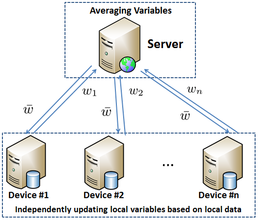
Figure 1: A star-network of FL system includes a server and multiple devices. In the basic FL problem (2), the server averages the local model variables $\bar{w}=\sum_{i=1}^{n}r_{i}w_{i}$, and sends $\bar{w}$ to each device; Each device update the local variable $w_{i}$ for $i\in[n]$, and then sent it to the server.

2.2 Composition Stochastic Optimization

Composition stochastic optimization has been widely applied to many applications such as reinforcement learning [33], model-agnostic meta Learning [34] and risk management [33]. Some compositional gradient methods have recently been proposed to solve these composition optimization problems. For example, stochastic compositional gradient methods [35, 33, 36] have been proposed to solve these problems. Subsequently, some variance-reduced compositional algorithms [37, 38, 39] have been proposed for composition optimization. More recently, [34, 40] presented a class of adaptive compositional gradient methods.

2.3 Model-Agnostic Meta Learning

Model-Agnostic Meta Learning (MAML) is an effective learning framework that learns a good initialization from prior experiences to fast adaptation in new tasks [7, 41]. MAML has been widely used to various applications such as deep learning [7], reinforcement learning [42, 43, 44] and personalized federated learning [8]. For example, [43] has proposed stochastic gradient meta-reinforcement learning, which can be regarded as a variant of the MAML method. [8] has studied a personalized variant of federated learning from the MAML view.

Due to solving MAML requires information on the stochastic Hessian matrix, some Hessian-free methods [45, 46] have been recently proposed to reduce the cost of computing Hessian matrix. At the same time, [47] studied the general multi-step MAML instead of one-step one to improve performance. More recently, [34, 40] have applied the composition optimization to the MAML by using the compositional structure of MAML.

Notations: $\|\cdot\|$ denotes the $\ell_{2}$ norm for vectors and spectral norm for matrices. $\langle x,y\rangle$ denotes the inner product of two vectors $x$ and $y$. $M^{T}$ denotes transpose of matrix $M$. For two sequences $\{a_{n}\}$ and $\{b_{n}\}$, we denote $a_{n}=O(b_{n})$ if $a_{n}\leq Cb_{n}$ for constant $C>0$.

3 Compositional Federated Learning

In this section, we propose an effective and efficient compositional federated learning (ComFedL) algorithm to solve the problem (1) based on compositional gradient descent iteration. The pseudo code of ComFedL algorithm is given in Algorithm 1.

Algorithm 1 Compositional Federated Learning (ComFedL) Algorithm

1:  Input: Synchronization gap $\tau$, number of outer iterations $S$, learning rate $\eta$, and initial parameter $\bar{w}_{0}\in\mathbb{R}^{d}$;

2:  for $s=0,1,\ldots,S-1$ do

3:     Server samples a mini-batch devices $\mathcal{C}_{s}\subset[n]$ with $|\mathcal{C}_{s}|=m$;

4:     Server broadcasts $\bar{w}_{s}$ to all devices $i\in\mathcal{C}_{s}$;

5:     for Devices $i\in\mathcal{C}_{s}$ parallel do

6:        Device sets $w^{i}_{s,0}=\bar{w}_{s}$;

7:        for $t=0,1,\cdots,\tau-1$ do

8:           Device draws a mini-batch samples $\mathcal{B}^{i}_{t}\subset\mathcal{D}_{i}$ with $|\mathcal{B}^{i}_{t}|=b$;

9:           Device computes $f^{i}_{\mathcal{B}^{i}_{t}}(w^{i}_{s,t})=\frac{1}{b}\sum_{j\in\mathcal{B}^{i}_{t}}f^{i}(w^{i}_{s,t};\xi_{j})$ and $\nabla f^{i}_{\mathcal{B}^{i}_{t}}(w^{i}_{s,t})=\frac{1}{b}\sum_{j\in\mathcal{B}^{i}_{t}}\nabla f^{i}(w^{i}_{s,t};\xi_{j})$;

10:           Device draws a mini-batch samples $\tilde{\mathcal{B}}^{i}_{t}\subset\tilde{\mathcal{D}}_{i}$ with $|\tilde{\mathcal{B}}^{i}_{t}|=b_{1}$;

11:           Device computes $\nabla g^{i}_{\tilde{\mathcal{B}}^{i}_{t}}(f^{i}_{\mathcal{B}^{i}_{t}}(w^{i}_{s,t}))=\frac{1}{b_{1}}\sum_{j\in\tilde{\mathcal{B}}^{i}_{t}}\nabla g^{i}(f^{i}_{\mathcal{B}^{i}_{t}}(w^{i}_{s,t});\zeta_{j})$;

12:           $u^{i}_{s,t}=\nabla g^{i}_{\tilde{\mathcal{B}}^{i}_{t}}(f^{i}_{\mathcal{B}^{i}_{t}}(w^{i}_{s,t}))^{T}\nabla f^{i}_{\mathcal{B}^{i}_{t}}(w^{i}_{s,t})$;

13:           $w^{i}_{s,t+1}=w^{i}_{s,t}-\eta u^{i}_{s,t}$;

14:        end for

15:        Device sends $w^{i}_{s,\tau}$ back to server;

16:     end for

17:     Server computes $\bar{w}_{s+1}=\frac{1}{m}\sum_{i\in\mathcal{C}_{s}}w^{i}_{s,\tau}$;

18:  end for

19:  Output: Final solution $w_{T}$.

For solving the problem (1), we should compute the gradient of composition function $F^{i}(w)=g^{i}(f^{i}(w))$, defined as

$$\nabla F^{i}(w)=\big{(}\nabla g^{i}(f^{i}(w))\big{)}^{T}\nabla f^{i}(w).$$ (11)

Since the inner function (or mapping) $y^{i}=f^{i}(w)=\mathbb{E}_{\xi\sim\mathcal{D}_{i}}f^{i}(w;\xi)$ and the outer function $g^{i}(y^{i})=\mathbb{E}_{\zeta\sim\tilde{\mathcal{D}}_{i}}f^{i}(y^{i};\zeta)$ are expected functions, we can not compute the full gradient $\nabla F^{i}(w)$. Thus, we compute the stochastic gradient $\nabla F^{i}(w)$ based on some mini-batch samples. Specifically, we draw a mini-batch samples $\mathcal{B}^{i}_{t}\subset\mathcal{D}_{i}$ with $|\mathcal{B}^{i}_{t}|=b$, and then compute stochastic value of inner function $f^{i}_{\mathcal{B}^{i}_{t}}(w^{i}_{s,t})=\frac{1}{b}\sum_{j\in\mathcal{B}^{i}_{t}}f^{i}(w^{i}_{s,t};\xi_{j})$ and its stochastic gradient $\nabla f^{i}_{\mathcal{B}^{i}_{t}}(w^{i}_{s,t})=\frac{1}{b}\sum_{j\in\mathcal{B}^{i}_{t}}\nabla f^{i}(w^{i}_{s,t};\xi_{j})$. At the same time, we draw a mini-batch samples $\tilde{\mathcal{B}}^{i}_{t}\subset\tilde{\mathcal{D}}_{i}$ with $|\tilde{\mathcal{B}}^{i}_{t}|=b_{1}$, and compute stochastic gradient of outer function $\nabla g^{i}_{\tilde{\mathcal{B}}^{i}_{t}}(f^{i}_{\mathcal{B}^{i}_{t}}(w^{i}_{s,t}))=\frac{1}{b_{1}}\sum_{j\in\tilde{\mathcal{B}}^{i}_{t}}g^{i}(f^{i}_{\mathcal{B}^{i}_{t}}(w^{i}_{s,t});\zeta_{j})$. Finally, we obtain the stochastic gradient estimator $u^{i}_{s,t}=\nabla g^{i}_{\tilde{\mathcal{B}}^{i}_{t}}(f^{i}_{\mathcal{B}^{i}_{t}}(w^{i}_{s,t}))^{T}\nabla f^{i}_{\mathcal{B}^{i}_{t}}(w^{i}_{s,t})$. Clearly, the gradient estimator $u^{i}_{s,t}$ is a biased estimator of $\nabla F^{i}(w)$, i.e., $\mathbb{E}[u^{i}_{s,t}]\neq\nabla F^{i}(w)$.

When the outer functions $\{g^{i}\}_{i=1}^{n}$ in the problem (1) are determinate and $g^{1}=g^{2}=\cdots=g^{n}$, i.e., $F^{i}(w)=g(\mathbb{E}[f^{i}(w;\xi)])$, we only compute stochastic gradient $u^{i}_{s,t}=\nabla g(f^{i}_{\mathcal{B}^{i}_{t}}(w^{i}_{s,t}))^{T}\nabla f^{i}_{\mathcal{B}^{i}_{t}}(w^{i}_{s,t})$. For example, by the following Lemma 1, we can obtain the simple composition problem (6) is similarly equivalent to the minimax problem (4) with $\phi(r,1/n)=\sum_{i=1}^{n}r_{i}\log(nr_{i})$. To solve the problem (6), we can obtain $u^{i}_{t}=\big{(}\exp\big{(}f^{i}_{\mathcal{B}^{i}_{t}}(w^{i}_{t})/\gamma\big{)}/\gamma\big{)}\nabla f^{i}_{\mathcal{B}^{i}_{t}}(w^{i}_{t})$.

When obtaining the stochastic gradient $u^{i}_{s,t}$, we will use the SGD to update the parameter $w$ given at the line 13 in Algorithm 1, where we can choose an appropriate learning rate $\eta>0$ to guarantee the convergence of our algorithm. In Algorithm 1, we apply the local-SGD framework to reduce communication. Specifically, our ComFedL algorithm performs multiple stochastic gradient descent (SGD) in the available devices before communicating to the server, which can reduce the total amount of communication. In Algorithm 1, we use the synchronization gap $\tau>0$ to control the communication cost and performances of our algorithm.

At the line 17 of Algorithm 1, the server averages the local model variables $\bar{w}_{s+1}=\frac{1}{m}\sum_{i\in\mathcal{C}_{s}}w^{i}_{s,\tau}$ as in the robust FL algorithms [5] instead of the re-weighting formulation $\bar{w}_{s+1}=\sum_{i\in\mathcal{C}_{s}}r_{i}w^{i}_{s,\tau}$ in the FedAvg algorithm [1]. Because our ComFedL solves the Distributionally Robust FL as a simpler compositional optimization problem, which is equivalent to a regularized minimax problem that searches for a global variable from the worst-case loss.

4 Theoretical Analysis

In this section, we first give a key lemma that shows the robust FL can be formed as a simple yet effective compositional optimization problem, and then provide the detailed convergence analysis of our ComFedL algorithm.

4.1 A Key Lemma

In this subsection, we introduce a useful lemma that shows the robust FL can be formed as a simple yet effective compositional optimization problem.

Lemma 1.

The above minimax problem (4) with $\phi(r,1/n)=\sum_{i=1}^{n}r_{i}\log(nr_{i})$, i.e.,

$$\min_{w\in\mathbb{R}^{d}}\max_{r\in\Lambda_{n}}\sum_{i=1}^{n}r_{i}f^{i}(w)-\gamma\sum_{i=1}^{n}r_{i}\log(nr_{i}),$$ (12)

$$\quad\mbox{s.t.}\ \Lambda_{n}=\big{\{}r\in\mathbb{R}^{n}_{+}\ |\ \sum_{i=1}^{n}r_{i}=1\big{\}}$$

is equivalent to the above composition problem (5), i.e.,

$$\min_{w\in\mathbb{R}^{d}}\gamma\log\bigg{(}\frac{1}{n}\sum_{i=1}^{n}\exp\big{(}f^{i}(w)/\gamma\big{)}\bigg{)}.$$ (13)

Proof.

We maximize the above problem (12) over $r\in\Lambda_{n}=\big{\{}r\in\mathbb{R}^{n}_{+}|\sum_{i=1}^{n}r_{i}=1\big{\}}$, i.e.,

$$\max_{r\in\Lambda_{n}}F(w,r):=\sum_{i=1}^{n}r_{i}f^{i}(w)-\gamma\sum_{i=1}^{n}r_{i}\log(r_{i}n).$$ (14)

For function $F(w,r)$, we first introduce its Lagrange function

$$L(w,r,\lambda)=\sum_{i=1}^{n}r_{i}f^{i}(w)\!-\!\gamma\sum_{i=1}^{n}r_{i}\log(r_{i}n)\!+\!\lambda\big{(}\sum_{i=1}^{n}r_{i}\!-\!1\big{)},$$

where $\lambda$ is a Lagrange multiplier. Then we have

$$\frac{\partial L(w,r,\lambda)}{\partial r_{i}}=f^{i}(w)-\gamma\log(r_{i}n)-\gamma+\lambda=0.$$ (15)

According to the equality (15), we have

$$f^{i}(w)-\gamma\log(nr_{i})=\gamma-\lambda.$$ (16)

Then by using the equality (16), we can obtain

$$r_{i}=\frac{1}{n}\exp(\frac{\lambda}{\gamma}-1)\exp(f^{i}(w)/\gamma)$$ (17)

According to $\sum_{i=1}^{n}r_{i}=1$, we have

$$\sum_{i=1}^{n}r_{i}=\frac{1}{n}\exp(\frac{\lambda}{\gamma}-1)\sum_{i=1}^{n}\exp(f^{i}(w)/\gamma)=1,$$ (18)

Clearly, we can obtain

$$\exp(1-\frac{\lambda}{\gamma})=\frac{1}{n}\sum_{i=1}^{n}\exp(f^{i}(w)/\gamma).$$ (19)

Taking the logarithm of its both sides, we have

$$1-\frac{\lambda}{\gamma}=\log\big{(}\frac{1}{n}\sum_{i=1}^{n}\exp(f^{i}(w)/\gamma)\big{)}.$$ (20)

According to $\sum_{i=1}^{n}r_{i}=1$ and the above equalities (16) and (20), we have

$$F(w,r) =\sum_{i=1}^{n}r_{i}\big{(}f^{i}(w)-\gamma\log(nr_{i})\big{)}=\gamma-\lambda$$

$$=\gamma\log\big{(}\frac{1}{n}\sum_{i=1}^{n}\exp(f^{i}(w)/\gamma)\big{)},$$ (21)

where the last equality is due to the above equality (20).

Thus, the above minimax problem (12) is equivalent to the above composition problem (13). In the other word, by exactly maximizing the above problem (4) over $r\in\Lambda_{n}$, the above minimax problem (4) with $\phi(r,1/n)=\sum_{i=1}^{n}r_{i}\log(nr_{i})$ is equivalent to the composition problem (5).

∎

4.2 Some Mild Assumptions

In this subsection, we introduce some mild conditions.

Assumption 1.

There exist constants $L_{f}$, $L_{g}$ and $L$ for $\nabla f^{i}(w;\xi)$, $\nabla g^{i}(y;\zeta)$ and $\nabla F(w)$ satisfying that for $i\in[n]$

$$\|\nabla f^{i}(w_{1};\xi)\!-\!\nabla f^{i}(w_{2};\xi)\|\!\leq\!L_{f}\|w_{1}\!-\!w_{2}\|,\forall w_{1},w_{2}\in\mathbb{R}^{d},$$

$$\|\nabla g^{i}(y_{1},\zeta)-\nabla g^{i}(y_{2},\zeta)\|\leq L_{g}\|y_{1}-y_{2}\|,\forall y_{1},y_{2}\in\mathbb{R}^{p},$$

$$\|\nabla F(w_{1})-\nabla F(w_{2})\|\leq L\|w_{1}-w_{2}\|,$$

and the last inequality follows

$$F(w_{2})\leq F(w_{1})+\nabla F(w_{1})^{T}(w_{2}-w_{1})+\frac{L}{2}\|w_{1}-w_{2}\|^{2}.$$

Assumption 2.

Gradient $\nabla g^{i}(y)$ and Jacobian matrix $\nabla f^{i}(w)$ have the upper bounds $G_{g}$ and $G_{f}$, respectively, i.e., for $i\in[n]$

$$\|\nabla f^{i}(w;\xi)\|\leq G_{f},\forall w\in\mathbb{R}^{d};\|\nabla g^{i}(y;\zeta)\|\leq G_{g},\forall y\in\mathbb{R}^{p}.$$

Assumption 3.

The variances of stochastic gradient or value of functions $f^{i}(w;\xi)$ and $g^{i}(y;\zeta)$, i.e., we have for all $i\in[n]$

$$\mathbb{E}\|\nabla f^{i}(w;\xi)-\nabla f^{i}(w)\|^{2}\leq\sigma_{1}^{2},$$

$$\mathbb{E}\|f^{i}(w;\xi)-f^{i}(w)\|^{2}\leq\sigma_{2}^{2},\ \forall w\in\mathbb{R}^{d}$$

$$\mathbb{E}\|\nabla g^{i}(y;\zeta)-\nabla g^{i}(y)\|^{2}\leq\sigma_{3}^{2},\ \forall y\in\mathbb{R}^{p}$$

where $\sigma_{1},\sigma_{2},\sigma_{3}>0$. Let $\sigma=\max(\sigma_{1},\sigma_{2},\sigma_{3})$.

Assumption 4.

$F(w)$ is lower bounded, i.e., $F^{*}=\inf_{w\in\mathbb{R}^{d}}F(w)$.

Assumptions 4.2-4.5 have been commonly used in the convergence analysis of the composition stochastic algorithms [35, 33]. Specifically, Assumption 4.2 ensures the smoothness of functions $f^{i}(w;\xi)$, $g^{i}(y;\zeta)$ and $F(w)$. Assumption 4.3 ensures the bounded gradients (or Jacobian matrix) of functions $f^{i}(w;\xi)$ and $g^{i}(y;\zeta)$. Assumption 4.4 ensures the bounded variances of stochastic gradient or value of functions $f^{i}(w;\xi)$ and $g^{i}(y;\zeta)$. Assumption 4.5 guarantees the feasibility of the problem (1). For the special problem (1), where the outer functions $\{g^{i}\}_{i=1}^{n}$ are determinate and $g^{1}=\cdots=g^{n}$, we only assume $\|\nabla g(y_{1})-\nabla g(y_{2})\|\leq L_{g}\|y_{1}-y_{2}\|,\ \forall y_{1},y_{2}\in\mathbb{R}^{p}$ and $\|\nabla g(y)\|\leq G_{g},\ \forall y\in\mathbb{R}^{p}$. For example, in the above problem (6), $g(y),\ y\in\mathcal{Y}$ is a monotonically increasing function, where $\mathcal{Y}$ is the range of functions $\{f^{i}(w)\}$. Thus, $g(y)$ is generally smooth and $\|\nabla g(y)\|$ is bounded. Note that we analyze the convergence properties of our ComFedL algorithm under non-i.i.d. and nonconvex setting. Although our convergence analysis relies on the bounded gradients in Assumption 4.4, the exiting convergence analysis of FL algorithms [19, 48, 49, 5] under non-i.i.d. and nonconvex (or strongly convex) setting also rely on the bounded gradients.

4.3 Convergence Analysis

In this subsection, we detail the convergence analysis of our CompFedL algorithm. In Algorithm 1, we only obtain a biased stochastic gradient in each device, due to the compositional loss function in our new FL framework. While the unbiased stochastic gradient is easily obtained in each device in the existing FL framework. Thus, our convergence analysis can not easily follow the existing convergence analysis of the FL [19, 14, 48]. For notational simplicity, let

$$\bar{w}_{s,t} =\frac{1}{m}\sum_{i\in\mathcal{C}_{s}}w^{i}_{s,t},$$

$$\bar{u}_{s,t} =\frac{1}{m}\sum_{i\in\mathcal{C}_{s}}u^{i}_{s,t}=\frac{1}{m}\sum_{i\in\mathcal{C}_{s}}\nabla g^{i}_{\tilde{\mathcal{B}}^{i}_{t}}(f^{i}_{\mathcal{B}^{i}_{t}}(w^{i}_{s,t}))^{T}\nabla f^{i}_{\mathcal{B}^{i}_{t}}(w^{i}_{s,t}),$$

then we have $\bar{w}_{s,t+1}=\bar{w}_{s,t}-\eta\bar{u}_{s,t}$. Let

$$U_{s,0}=\frac{1}{m}\sum_{i\in\mathcal{C}_{s}}\nabla F^{i}(\bar{w}_{s})=\frac{1}{m}\sum_{i\in\mathcal{C}_{s}}\nabla g^{i}\big{(}f^{i}(\bar{w}_{s})\big{)}^{T}\nabla f^{i}(\bar{w}_{s}),$$ (22)

we have $\mathbb{E}[U_{s,0}]=\nabla F(\bar{w}_{s})$.

Lemma 2.

Under the about Assumptions, we have

$$\mathbb{E}\|\bar{w}_{s,t}-\bar{w}_{s}\|^{2}\leq\tau^{2}\eta^{2}G^{2}_{g}G^{2}_{f}.$$

Proof.

Since $\bar{w}_{s}=w^{i}_{s,0}$, we have

$$\mathbb{E}\|\bar{w}_{s,t}-\bar{w}_{s}\|^{2}=\mathbb{E}\|\frac{1}{m}\sum_{i\in\mathcal{C}_{s}}w^{i}_{s,t}-\bar{w}_{s}\|^{2}$$

$$\leq\frac{1}{m}\sum_{i\in\mathcal{C}_{s}}\mathbb{E}\|w^{i}_{s,t}-\bar{w}_{s}\|^{2}=\frac{1}{m}\sum_{i\in\mathcal{C}_{s}}\mathbb{E}\|w^{i}_{s,t}-w^{i}_{s,0}\|^{2}$$

$$=\frac{1}{m}\sum_{i\in\mathcal{C}_{s}}\mathbb{E}\|\sum_{j=0}^{t-1}\eta u^{i}_{s,j}\|^{2}$$

$$\leq\frac{1}{m}\sum_{i\in\mathcal{C}_{s}}\bigg{(}t\eta^{2}\sum_{j=0}^{t-1}\mathbb{E}\|\nabla g_{\tilde{\mathcal{B}}^{i}_{t}}(f^{i}_{\mathcal{B}^{i}_{t}}(w^{i}_{s,t}))^{T}\nabla f^{i}_{\mathcal{B}^{i}_{t}}(w^{i}_{s,t})\|^{2}\bigg{)}$$

$$\leq t^{2}\eta^{2}G^{2}_{g}G^{2}_{f}\leq\tau^{2}\eta^{2}G^{2}_{g}G^{2}_{f},$$ (23)

where the second inequality holds by Assumption 2. ∎

Lemma 3.

Under the above Assumptions, we have

$$\mathbb{E}\|\bar{u}_{s,t}-U_{s,0}\|^{2}\leq 5(G^{2}_{g}L^{2}_{f}+G^{4}_{f}L^{2}_{g})\tau^{2}\eta^{2}G^{2}_{g}G^{2}_{f}$$

$$\quad+\frac{5G^{2}_{f}\sigma^{2}}{b_{1}}+\frac{5G^{2}_{g}\sigma^{2}}{b}+\frac{5L_{g}^{2}G_{f}^{2}\sigma^{2}}{b}.$$ (24)

Proof.

By using the above equality (22), we have

$$\mathbb{E}\|\bar{u}_{s,t}-U_{s,0}\|^{2}$$

$$=\mathbb{E}\|\frac{1}{m}\sum_{i\in\mathcal{C}_{s}}\nabla g^{i}_{\tilde{\mathcal{B}}^{i}_{t}}(f^{i}_{\mathcal{B}^{i}_{t}}(w^{i}_{s,t}))^{T}\nabla f^{i}_{\mathcal{B}^{i}_{t}}(w^{i}_{s,t})$$

$$\ -\nabla g^{i}(f^{i}(\bar{w}_{s}))^{T}\nabla f^{i}(\bar{w}_{s})\|^{2}$$

$$\leq\frac{1}{m}\sum_{i\in\mathcal{C}_{s}}\mathbb{E}\|\nabla g^{i}_{\tilde{\mathcal{B}}^{i}_{t}}(f^{i}_{\mathcal{B}^{i}_{t}}(w^{i}_{s,t}))^{T}\nabla f^{i}_{\mathcal{B}^{i}_{t}}(w^{i}_{s,t})$$

$$\ -\nabla g^{i}(f^{i}(\bar{w}_{s}))^{T}\nabla f^{i}(\bar{w}_{s})\|^{2}$$

$$=\frac{1}{m}\sum_{i\in\mathcal{C}_{s}}\mathbb{E}\|\nabla g^{i}_{\tilde{\mathcal{B}}^{i}_{t}}(f^{i}_{\mathcal{B}^{i}_{t}}(w^{i}_{s,t}))^{T}\nabla f^{i}_{\mathcal{B}^{i}_{t}}(w^{i}_{s,t})$$

$$\ -\nabla g^{i}_{\tilde{\mathcal{B}}^{i}_{t}}(f^{i}_{\mathcal{B}^{i}_{t}}(w^{i}_{s,t}))^{T}\nabla f^{i}_{\mathcal{B}^{i}_{t}}(\bar{w}_{s})$$

$$\ +\nabla g^{i}_{\tilde{\mathcal{B}}^{i}_{t}}(f^{i}_{\mathcal{B}^{i}_{t}}(w^{i}_{s,t}))^{T}\nabla f^{i}_{\mathcal{B}^{i}_{t}}(\bar{w}_{s})\!-\!\nabla g^{i}(f^{i}_{\mathcal{B}^{i}_{t}}(w^{i}_{s,t}))^{T}\nabla f^{i}_{\mathcal{B}^{i}_{t}}(\bar{w}_{s})$$

$$\ +\nabla g^{i}(f^{i}_{\mathcal{B}^{i}_{t}}(w^{i}_{s,t}))^{T}\nabla f^{i}_{\mathcal{B}^{i}_{t}}(\bar{w}_{s})-\nabla g^{i}(f^{i}_{\mathcal{B}^{i}_{t}}(w^{i}_{s,t}))^{T}\nabla f^{i}(\bar{w}_{s})$$

$$\ +\nabla g^{i}(f^{i}_{\mathcal{B}^{i}_{t}}(w^{i}_{s,t}))^{T}\nabla f^{i}(\bar{w}_{s})-\nabla g^{i}(f^{i}_{\mathcal{B}^{i}_{t}}(\bar{w}_{s}))^{T}\nabla f^{i}(\bar{w}_{s})$$

$$\ +\nabla g^{i}(f^{i}_{\mathcal{B}^{i}_{t}}(\bar{w}_{s}))^{T}\nabla f^{i}(\bar{w}_{s})-\nabla g^{i}(f^{i}(\bar{w}_{s}))^{T}\nabla f^{i}(\bar{w}_{s})\|^{2}$$

$$\leq\frac{5G^{2}_{g}L^{2}_{f}}{m}\sum_{i\in\mathcal{C}_{s}}\mathbb{E}\|w^{i}_{s,t}-\bar{w}_{s}\|^{2}+\frac{5G^{2}_{f}\sigma^{2}}{b_{1}}+\frac{5G^{2}_{g}\sigma^{2}}{b}$$

$$\ +\frac{5G^{4}_{f}L^{2}_{g}}{m}\sum_{i\in\mathcal{C}_{s}}\mathbb{E}\|w^{i}_{s,t}-\bar{w}_{s}\|^{2}+\frac{5L_{g}^{2}G_{f}^{2}\sigma^{2}}{b}$$

$$\leq 5(G^{2}_{g}L^{2}_{f}+G^{4}_{f}L^{2}_{g})\tau^{2}\eta^{2}G^{2}_{g}G^{2}_{f}+\frac{5G^{2}_{f}\sigma^{2}}{b_{1}}$$

$$\ +\frac{5G^{2}_{g}\sigma^{2}}{b}+\frac{5L_{g}^{2}G_{f}^{2}\sigma^{2}}{b},$$ (25)

where the second inequality is due to Assumptions 1-3, and the last inequality holds by Lemma 2. ∎

Theorem 1.

Under the above assumptions, in Algorithm 1, given $\eta>0$ and $b=b_{1}>0$, we have

$$\frac{1}{S}\sum_{s=0}^{S-1}\mathbb{E}\|\nabla F(\bar{w}_{s})\|^{2}$$

$$\leq\frac{F(\bar{w}_{0})-F^{*}}{T\eta}+G_{f}G_{g}\bigg{(}\sqrt{5}H\tau G_{g}G_{f}\eta\frac{\sqrt{5}G_{f}\sigma}{\sqrt{b_{1}}}$$

$$\ +\frac{\sqrt{5}G_{g}\sigma}{\sqrt{b}}+\frac{\sqrt{5}L_{g}G_{f}\sigma}{\sqrt{b}}\bigg{)}+L\tau\eta G^{2}_{g}G^{2}_{f}+\frac{L\eta}{2}G_{f}^{2}G_{g}^{2},$$ (26)

where $T=\tau S$ and $H=\sqrt{G^{2}_{g}L^{2}_{f}+G^{4}_{f}L^{2}_{g}}$.

Proof.

By the smoothness of the function $F(x)$, we have

$$\mathbb{E}[F(\bar{w}_{s,t+1})]$$

$$\leq\mathbb{E}[F(\bar{w}_{s,t})]+\mathbb{E}\langle\nabla F(\bar{w}_{s,t}),\bar{w}_{s,t+1}-\bar{w}_{s,t}\rangle$$

$$\quad+\frac{L}{2}\mathbb{E}\|\bar{w}_{s,t+1}-\bar{w}_{s,t}\|^{2}$$

$$=\mathbb{E}[F(\bar{w}_{s,t})]+\mathbb{E}\langle\nabla F(\bar{w}_{s,t}),-\eta\bar{u}_{s,t}\rangle+\frac{L}{2}\mathbb{E}\|\eta\bar{u}_{s,t}\|^{2}$$

$$=\mathbb{E}[F(\bar{w}_{s,t})]-\eta\mathbb{E}\langle\nabla F(\bar{w}_{s,t}),\bar{u}_{s,t}-U_{s,0}\rangle$$

$$\quad-\eta\mathbb{E}\langle\nabla F(\bar{w}_{s,t})-\nabla F(\bar{w}_{s}),U_{s,0}\rangle-\eta\mathbb{E}\langle\nabla F(\bar{w}_{s}),U_{s,0}\rangle$$

$$\quad+\frac{L}{2}\mathbb{E}\|\eta\bar{u}_{s,t}\|^{2}$$

$$\leq\mathbb{E}[F(\bar{w}_{s,t})]+\eta\mathbb{E}\big{(}\|\nabla F(\bar{w}_{s,t})\|\|\bar{u}_{s,t}-U_{s,0}\|\big{)}$$

$$\quad+\eta\mathbb{E}\big{(}\|\nabla F(\bar{w}_{s,t})-\nabla F(\bar{w}_{s})\|\|U_{s,0}\|\big{)}-\eta\mathbb{E}\|\nabla F(\bar{w}_{s})\|^{2}$$

$$\quad+\frac{L\eta^{2}}{2}\mathbb{E}\|\bar{u}_{s,t}\|^{2}$$

$$\leq\mathbb{E}[F(\bar{w}_{s,t})]+\eta G_{f}G_{g}\mathbb{E}\|\bar{u}_{s,t}-U_{s,0}\|+\eta LG_{f}G_{g}\mathbb{E}\|\bar{w}_{s,t}-\bar{w}_{s}\|$$

$$\quad-\eta\mathbb{E}\|\nabla F(\bar{w}_{s})\|^{2}+\frac{L\eta^{2}}{2}G_{f}^{2}G_{g}^{2}$$

$$\leq\mathbb{E}[F(\bar{w}_{s,t})]+\eta G_{f}G_{g}\sqrt{\mathbb{E}\|\bar{u}_{s,t}-U_{s,0}\|^{2}}$$

$$\quad+\eta LG_{f}G_{g}\sqrt{\mathbb{E}\|\bar{w}_{s,t}-\bar{w}_{s}\|^{2}}-\eta\mathbb{E}\|\nabla F(\bar{w}_{s})\|^{2}+\frac{L\eta^{2}}{2}G_{f}^{2}G_{g}^{2}$$

$$\leq\mathbb{E}[F(\bar{w}_{s,t})]+\eta G_{f}G_{g}\bigg{(}\sqrt{5(G^{2}_{g}L^{2}_{f}+G^{4}_{f}L^{2}_{g})}\tau\eta G_{g}G_{f}$$

$$\quad+\frac{\sqrt{5}G_{f}\sigma}{\sqrt{b_{1}}}+\frac{\sqrt{5}G_{g}\sigma}{\sqrt{b}}+\frac{\sqrt{5}L_{g}G_{f}\sigma}{\sqrt{b}}\bigg{)}+L\tau\eta^{2}G^{2}_{g}G^{2}_{f}$$

$$\quad-\eta\mathbb{E}\|\nabla F(\bar{w}_{s})\|^{2}+\frac{L\eta^{2}}{2}G_{f}^{2}G_{g}^{2},$$ (27)

where the second inequality is due to Cauchy-Schwarz inequality and $\mathbb{E}[U_{s,0}]=\nabla F(\bar{w}_{s})$; the second last inequality holds by the concavity of $\sqrt{x}$, and the last inequality is due to Lemmas 2 and 3. Thus, we have

$$\eta\mathbb{E}\|\nabla F(\bar{w}_{s})\|^{2}\leq\mathbb{E}[F(\bar{w}_{s,t})]-\mathbb{E}[F(\bar{w}_{s,t+1})]$$

$$\ +\eta G_{f}G_{g}\bigg{(}\sqrt{5(G^{2}_{g}L^{2}_{f}+G^{4}_{f}L^{2}_{g})}\tau\eta G_{g}G_{f}\!+\!\frac{\sqrt{5}G_{f}\sigma}{\sqrt{b_{1}}}\!+\!\frac{\sqrt{5}G_{g}\sigma}{\sqrt{b}}$$

$$\ +\frac{\sqrt{5}L_{g}G_{f}\sigma}{\sqrt{b}}\bigg{)}+L\tau\eta^{2}G^{2}_{g}G^{2}_{f}+\frac{L\eta^{2}}{2}G_{f}^{2}G_{g}^{2}.$$ (28)

Since $w_{s,0}=\bar{w}_{s}$, telescoping the above inequality over $s=0,1,\cdots,S-1$ and $t=0,1,\cdots,\tau-1$, we have

$$\frac{1}{S}\sum_{s=0}^{S-1}\mathbb{E}\|\nabla F(\bar{w}_{s})\|^{2}$$ (29)

$$\leq\frac{F(\bar{w}_{0})-F(\bar{w}_{T})}{T\eta}+G_{f}G_{g}\bigg{(}\sqrt{5(G^{2}_{g}L^{2}_{f}+G^{4}_{f}L^{2}_{g})}\tau\eta G_{g}G_{f}$$

$$\ +\frac{\sqrt{5}G_{f}\sigma}{\sqrt{b_{1}}}\!+\!\frac{\sqrt{5}G_{g}\sigma}{\sqrt{b}}\!+\!\frac{\sqrt{5}L_{g}G_{f}\sigma}{\sqrt{b}}\bigg{)}\!+\!L\eta G^{2}_{g}G^{2}_{f}\tau\!+\!\frac{L\eta}{2}G_{f}^{2}G_{g}^{2}$$

$$\leq\frac{F(\bar{w}_{0})-F^{*}}{T\eta}+G_{f}G_{g}\bigg{(}\sqrt{5(G^{2}_{g}L^{2}_{f}+G^{4}_{f}L^{2}_{g})}\tau\eta G_{g}G_{f}$$

$$\ +\frac{\sqrt{5}G_{f}\sigma}{\sqrt{b_{1}}}\!+\!\frac{\sqrt{5}G_{g}\sigma}{\sqrt{b}}\!+\!\frac{\sqrt{5}L_{g}G_{f}\sigma}{\sqrt{b}}\bigg{)}\!+\!L\tau\eta G^{2}_{g}G^{2}_{f}\!+\!\frac{L\eta}{2}G_{f}^{2}G_{g}^{2},$$

where the last inequality is due to Assumption 4. ∎

Remark 1.

Let $\eta=\frac{1}{T^{\alpha_{1}}},\ 0<\alpha_{1}\leq 1$, $b=\frac{1}{T^{\alpha_{2}}},\ \alpha_{2}>0$ and $b_{1}=\frac{1}{T^{\alpha_{3}}},\ \alpha_{3}>0$, we have $\frac{1}{S}\sum_{s=0}^{S-1}\mathbb{E}\|\nabla F(\bar{w}_{s})\|^{2}\leq O(\frac{1}{T^{1-\alpha_{1}}}+\frac{\tau}{T^{\alpha_{1}}}+\frac{1}{T^{0.5\alpha_{2}}}+\frac{1}{T^{0.5\alpha_{3}}})$. Thus, our ComFedL algorithm has a convergence rate of $O(\frac{1}{T^{1-\alpha_{1}}}+\frac{\tau}{T^{\alpha_{1}}}+\frac{1}{T^{0.5\alpha_{2}}}+\frac{1}{T^{0.5\alpha_{3}}})$. When $\alpha_{1}=\frac{1}{2}$, $\alpha_{2}=\alpha_{3}=1$ and $\tau=O(1)$, our ComFedL algorithm reaches a convergence rate of $O(\frac{1}{\sqrt{T}})$.

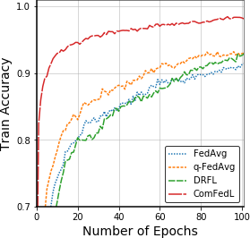
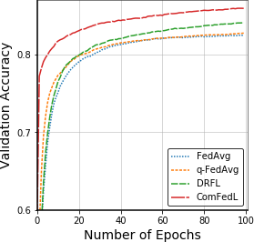
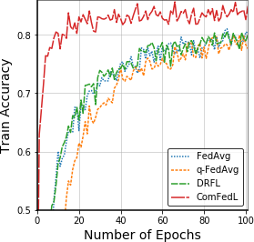
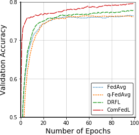
Figure 2: Train and Validation accuracy over imbalanced MNIST dataset with different robust FL methods. The top figures show average accuracy, and the bottom figures show the worst accuracy.

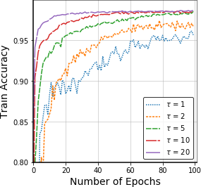
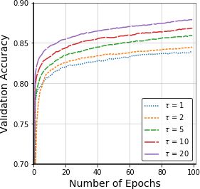
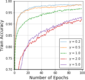
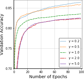
Figure 3: Comparing the effects of synchronization gap $\tau$ (top row) and regularization parameter $\gamma$ (bottom row) to our algorithm.

5 Experiments

In this section, we empirically validate the efficacy of our ComFedL algorithm. Specifically, we apply our algorithm to two tasks i.e. Distributionally Robust Federated Learning and Distribution Agnostic MAML-based Personalized Federated Learning. In the experiments, all algorithms are implemented based on the Distributed Library of Pytorch [50], and all experiments are run over a machine with 4 NVIDIA P40 GPUs.

5.1 Distributionally Robust Federated Learning

In this subsection, we conduct the distributionally robust FL task to verify effectiveness of our algorithm. In this set of experiments, we consider the multi-class classification problem over the MNIST [51] dataset with logistic regression model. The experiments are run over 10 clients and 1 server. In particular, we randomly select one client to have 5000 images, while the remained clients are distributed much less data, which is 20 images. This way of data construction is aimed to create imbalance among different client’s datasets. To get a good performance over this type of imbalanced datasets, the algorithm needs to attach more importance over the hardest task, i.e. the client that has dominant number of images. So it is a good way to test the ability of our algorithm to adapt to such imbalance.

We compare our algorithm with several state-of-the-art distributionally robust federated learning algorithms. In particular, we compare with DRFL [5], q-FedAvg [52] and the basic FedAvg [1]. In experiments, we set synchronization gap as 5 for all methods. As for other hyper-parameters, we perform grid search to find the optimal ones for each method and the search space is included in the following subsection 5.3. More specifically, Learning rate is 0.01 for all methods. In our algorithm, regularization parameter $\gamma$ is 0.2. In DRFL, client weights learning rate $\gamma$ is $8\times 10^{-2}$. In q-FedAvg, $q$ is set as 0.2. Finally, the synchronization gap is 5 by default. For all ablation studies, the hyper-parameters are chosen as above if not specified.

We show the result in Figure 2, where we report both average accuracy and the worst accuracy (among all the clients). As shown by the figure, our algorithm significantly outperforms all baselines in both metrics. Note that the FedAvg algorithm assigns weights proportional to the number of samples at each client, which might lead to bad validation performance for clients with smaller number of images (e.g. clients with only 20 images). Furthermore, DRFL solves a challenging minimax problem by optimizing the weight $r_{i}$ explicitly, while our algorithm can dynamically adjust the weight of clients, which makes our model simpler to train. Then in Figure 3, we show the robustness of our algorithm by varying the synchronization gap $\tau$ and the regularization parameter $\gamma$. As shown by the figure, our algorithm can get good train and validation accuracy with different values of $\tau$, furthermore, the algorithm converges much faster when we increase $\tau$, which shows the effectiveness of running multiple local epochs. Next, we show the effects of $\gamma$. Recall that $\gamma$ is a regularization parameter that penalizes the divergence $\phi(r,1/n)$. The larger $\gamma$ is, the more the algorithm emphasizes on getting $r_{i}$ close to the the average weight $\frac{1}{n}$. Since in our data-set, the optimal weights are far from $\frac{1}{n}$, we should pick $\gamma$ relatively small. This is verified by the results in Figure 3. The algorithm converges much faster when we choose $\gamma=0.1/0.2$ compared to that of $2/5$ in terms of both train and validation accuracy.

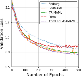
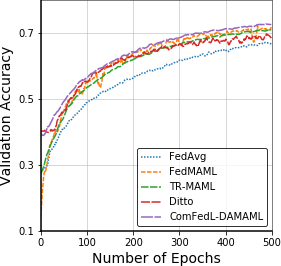
Figure 4: Validation loss (left) and Validation accuracy (right) over heterogeneous CIFAR-10 dataset with different personalized FL methods.

5.2 Distribution Agnostic MAML-based Personalized Federated Learning

In this subsection, we conduct Distribution Agnostic MAML-based personalized federated learning task to verify efficacy of our algorithm. Here we let ComFedL-DAMAML denote our algorithm for solving the above problem (10), i.e., a distributionally robust MAML-based personalized FL problem with regularization problem. We compare with the following baselines: FedAvg [1], FedMAML [8], TR-MAML [9] and Ditto [28]. In this set of experiments, we consider the multi-class classification task over the CIFAR10 [53] dataset with a 4-layer Convolutional Neural Network (CNN) used in [7]. We create the heterogeneous training (validation) dataset as follows: we create 10 clients and 1 server, while the dataset over each client includes images from a dominant class and a small percentage of images from other classes. The dominant class is different for different clients. More precisely, client-$i$ owns $\rho$ percentage images of class-$i$, and $(1-\rho)/9$ for other classes. For $\rho>0.1$ the images of each client will be dominated by a different class. The data distribution of each client is heterogeneous by construction, so it brings extra benefit by tuning a personalized model over each client. For all methods, we perform grid search to find the optimal hyper-parameters and the search space is reported in the following subsection 5.3. For FedAvg, the learning rate is 0.1; For FedMAML, both the inner and outer learning rate is 0.1; For TR-MAML, the inner learning rate is 0.05 and the outer learning rate is 0.1, while the learning rate of client weights is 0.08; For Ditto, the optimal learning rate for both the global and local models are 0.2, and the regularization parameter $\lambda$ is 0.1. For our ComFedL-DAMAML, the inner learning rate is set as 0.05, outer learning rate is 0.1 and the regularization parameter $\gamma$ is 0.5. Finally, the heterogeneity parameter $\rho$ is 0.28 and the synchronization gap is 5 by default. For all ablation studies, the hyper-parameters are chosen as above if not specified.

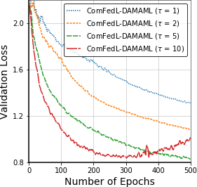
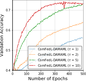
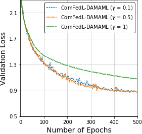
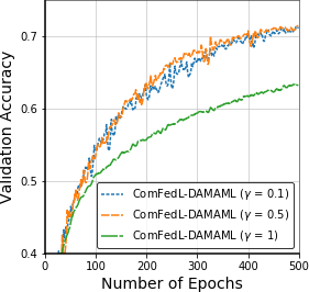
Figure 5: Comparing the effects of synchronization gap $\tau$ (top row) and regularization parameter $\gamma$ (bottom row) over ComFedL-DAMAML.

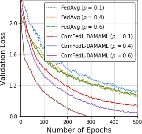
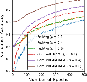
Figure 6: Comparing the effects of data heterogeneity $\rho$ over ComFedL-DAMAML.

In Figure 4, we compare ComFedL-DAMAML with other baseline methods. For fair comparison, FedAvg is trained with one step at test time. As shown by the figures, ComFedL-DAMAML outperforms other baselines. The basic FedAvg algorithm can not adapt to the heterogeneity of clients well and get the worst validation loss (accuracy). FedMAML and Ditto perform better but the loss (accuracy) curve is very noisy. TR-MAML gets a smoother curve compared to FedMAML due to its better balance of different clients. While our method outperforms all these methods. Our ComFedL-DAMAML algorithm adaptively adjusts the weight of clients based on the task’s performance (training loss). In other words, if the data distribution of a client is hard to learn (higher training loss), the algorithm increases its learning rate, while for clients with easier distributions, the learning rate is decreased. In summary, the results show that our ComFedL-DAMAML can also accelerate the personalized FL.

What’s more, we also test the effect of synchronization gap $\tau$ as shown in the top row of Figure 5. As shown in the figure, ComFedL-DAMAML converges much faster when we increase $\tau$, this shows the effectiveness of running multiple local epochs. Then in the bottom row of Figure 5, we compare effects of different regularization parameter $\gamma$. As shown by experiments, our algorithm is pretty robust with different values of $\gamma$. Finally, we test the effect of heterogeneity coefficient $\rho$ in Figure 6. $\rho$ represents the data heterogeneity among the clients, the larger $\rho$ is, the greater data heterogeneity. As shown by the figure, ComFedL-MAML consistently outperforms the FedAvg method over different $\rho$, especially when $\rho$ is large.

5.3 Hyper-parameter selection in the experiments

In the above Distributionally Robust Federated Learning experiments: For the learning rate, we search from [0.001, 0.01, 0.05, 0.1, 0.2, 0.5, 1]. We observe that when learning rate is 1, most methods just diverge. For our method, we search the regularization parameter from [0.1, 0.5, 1, 5]; For DRFL, we search the client weights learning rate from [8e-3, 8e-2, 8e-1]. For q-FedAvg, we search the $q$ value from [0.1, 0.2, 0.5, 1, 2].

In the above Distribution Agnostic MAML-based Personalized Federated Learning experiments: For the learning rate (both inner and outer if two types of learning rates are needed), we search from [0.001, 0.01, 0.05, 0.1, 0.2, 0.5, 1]. For our method, we search the regularization parameter from [0.1, 0.5, 1, 5]; For TR-MAML, we search the client weights learning rate from [8e-3, 8e-2, 8e-1]; For Ditto, we search the regularization parameter $\lambda$ from [0.05, 0.1, 0.5, 1, 5]

6 Conclusion

In the paper, we introduced a new compositional FL framework, and proposed an effective and efficient compositional FL (ComFedL) algorithm for solving this compositional FL framework. To the best of our knowledge, our new compositional FL is the first work to bridge federated learning with composition stochastic optimization. In particular, we first transform the distributionally robust federated learning (i.e., a minimax problem) into a simple composition problem by using KL divergence regularization.

References

• [1] B. McMahan, E. Moore, D. Ramage, S. Hampson, and B. A. y Arcas, “Communication-efficient learning of deep networks from decentralized data,” in Artificial Intelligence and Statistics.   PMLR, 2017, pp. 1273–1282.
• [2] P. Kairouz, H. B. McMahan, B. Avent, A. Bellet, M. Bennis, A. N. Bhagoji, K. Bonawitz, Z. Charles, G. Cormode, R. Cummings et al., “Advances and open problems in federated learning,” arXiv preprint arXiv:1912.04977, 2019.
• [3] M. Mohri, G. Sivek, and A. T. Suresh, “Agnostic federated learning,” in International Conference on Machine Learning.   PMLR, 2019, pp. 4615–4625.
• [4] A. Reisizadeh, F. Farnia, R. Pedarsani, and A. Jadbabaie, “Robust federated learning: The case of affine distribution shifts,” in NeurIPS, 2020.
• [5] Y. Deng, M. M. Kamani, and M. Mahdavi, “Distributionally robust federated averaging,” Advances in Neural Information Processing Systems, vol. 33, 2020.
• [6] M. Andrychowicz, M. Denil, S. G. Colmenarejo, M. W. Hoffman, D. Pfau, T. Schaul, B. Shillingford, and N. de Freitas, “Learning to learn by gradient descent by gradient descent,” in Proceedings of the 30th International Conference on Neural Information Processing Systems, 2016, pp. 3988–3996.
• [7] C. Finn, P. Abbeel, and S. Levine, “Model-agnostic meta-learning for fast adaptation of deep networks,” in International Conference on Machine Learning.   PMLR, 2017, pp. 1126–1135.
• [8] A. Fallah, A. Mokhtari, and A. Ozdaglar, “Personalized federated learning: A meta-learning approach,” arXiv preprint arXiv:2002.07948, 2020.
• [9] L. Collins, A. Mokhtari, and S. Shakkottai, “Distribution-agnostic model-agnostic meta-learning,” arXiv preprint arXiv:2002.04766, 2020.
• [10] Q. Yang, J. Zhang, W. Hao, G. Spell, and L. Carin, “Flop: Federated learning on medical datasets using partial networks,” arXiv preprint arXiv:2102.05218, 2021.
• [11] F. Haddadpour, M. M. Kamani, M. Mahdavi, and V. Cadambe, “Trading redundancy for communication: Speeding up distributed sgd for non-convex optimization,” in International Conference on Machine Learning.   PMLR, 2019, pp. 2545–2554.
• [12] F. Haddadpour, M. M. Kamani, M. Mahdavi, and V. R. Cadambe, “Local sgd with periodic averaging: Tighter analysis and adaptive synchronization,” arXiv preprint arXiv:1910.13598, 2019.
• [13] B. Woodworth, K. K. Patel, S. Stich, Z. Dai, B. Bullins, B. Mcmahan, O. Shamir, and N. Srebro, “Is local sgd better than minibatch sgd?” in International Conference on Machine Learning.   PMLR, 2020, pp. 10 334–10 343.
• [14] A. Khaled, K. Mishchenko, and P. Richtárik, “Tighter theory for local sgd on identical and heterogeneous data,” in International Conference on Artificial Intelligence and Statistics.   PMLR, 2020, pp. 4519–4529.
• [15] X. Liang, S. Shen, J. Liu, Z. Pan, E. Chen, and Y. Cheng, “Variance reduced local sgd with lower communication complexity,” arXiv preprint arXiv:1912.12844, 2019.
• [16] H. Yu, S. Yang, and S. Zhu, “Parallel restarted sgd with faster convergence and less communication: Demystifying why model averaging works for deep learning,” in Proceedings of the AAAI Conference on Artificial Intelligence, vol. 33, no. 01, 2019, pp. 5693–5700.
• [17] D. A. E. Acar, Y. Zhao, R. Matas, M. Mattina, P. Whatmough, and V. Saligrama, “Federated learning based on dynamic regularization,” in International Conference on Learning Representations, 2020.
• [18] S. P. Karimireddy, S. Kale, M. Mohri, S. J. Reddi, S. U. Stich, and A. T. Suresh, “Scaffold: Stochastic controlled averaging for on-device federated learning,” arXiv preprint arXiv:1910.06378, 2019.
• [19] X. Li, K. Huang, W. Yang, S. Wang, and Z. Zhang, “On the convergence of fedavg on non-iid data,” arXiv preprint arXiv:1907.02189, 2019.
• [20] A. K. Sahu, T. Li, M. Sanjabi, M. Zaheer, A. Talwalkar, and V. Smith, “On the convergence of federated optimization in heterogeneous networks,” arXiv preprint arXiv:1812.06127, vol. 3, 2018.
• [21] Y. Zhao, M. Li, L. Lai, N. Suda, D. Civin, and V. Chandra, “Federated learning with non-iid data,” arXiv preprint arXiv:1806.00582, 2018.
• [22] T. Li, A. K. Sahu, M. Zaheer, M. Sanjabi, A. Talwalkar, and V. Smith, “Federated optimization in heterogeneous networks,” arXiv preprint arXiv:1812.06127, 2018.
• [23] T.-M. H. Hsu, H. Qi, and M. Brown, “Measuring the effects of non-identical data distribution for federated visual classification,” arXiv preprint arXiv:1909.06335, 2019.
• [24] J. Wang, V. Tantia, N. Ballas, and M. Rabbat, “Slowmo: Improving communication-efficient distributed sgd with slow momentum,” arXiv preprint arXiv:1910.00643, 2019.
• [25] S. P. Karimireddy, M. Jaggi, S. Kale, M. Mohri, S. J. Reddi, S. U. Stich, and A. T. Suresh, “Mime: Mimicking centralized stochastic algorithms in federated learning,” arXiv preprint arXiv:2008.03606, 2020.
• [26] C. Xie, S. Koyejo, and I. Gupta, “Asynchronous federated optimization,” arXiv preprint arXiv:1903.03934, 2019.
• [27] H.-Y. Chen and W.-L. Chao, “On bridging generic and personalized federated learning,” arXiv preprint arXiv:2107.00778, 2021.
• [28] T. Li, S. Hu, A. Beirami, and V. Smith, “Ditto: Fair and robust federated learning through personalization,” in International Conference on Machine Learning.   PMLR, 2021, pp. 6357–6368.
• [29] Y. Jiang, J. Konečnỳ, K. Rush, and S. Kannan, “Improving federated learning personalization via model agnostic meta learning,” arXiv preprint arXiv:1909.12488, 2019.
• [30] Y. Deng, M. M. Kamani, and M. Mahdavi, “Adaptive personalized federated learning,” arXiv preprint arXiv:2003.13461, 2020.
• [31] C. T. Dinh, N. H. Tran, and T. D. Nguyen, “Personalized federated learning with moreau envelopes,” arXiv preprint arXiv:2006.08848, 2020.
• [32] F. Chen, M. Luo, Z. Dong, Z. Li, and X. He, “Federated meta-learning with fast convergence and efficient communication,” arXiv preprint arXiv:1802.07876, 2018.
• [33] M. Wang, J. Liu, and E. X. Fang, “Accelerating stochastic composition optimization,” The Journal of Machine Learning Research, vol. 18, no. 1, pp. 3721–3743, 2017.
• [34] R. Tutunov, M. Li, J. Wang, and H. Bou-Ammar, “Compositional adam: An adaptive compositional solver,” arXiv preprint arXiv:2002.03755, 2020.
• [35] M. Wang, E. X. Fang, and H. Liu, “Stochastic compositional gradient descent: algorithms for minimizing compositions of expected-value functions,” Mathematical Programming, vol. 161, no. 1-2, pp. 419–449, 2017.
• [36] S. Ghadimi, A. Ruszczynski, and M. Wang, “A single timescale stochastic approximation method for nested stochastic optimization,” SIAM Journal on Optimization, vol. 30, no. 1, pp. 960–979, 2020.
• [37] Z. Huo, B. Gu, J. Liu, and H. Huang, “Accelerated method for stochastic composition optimization with nonsmooth regularization,” in Proceedings of the AAAI Conference on Artificial Intelligence, vol. 32, no. 1, 2018.
• [38] T. Lin, C. Fan, M. Wang, and M. I. Jordan, “Improved sample complexity for stochastic compositional variance reduced gradient,” arXiv preprint arXiv:1806.00458, 2018.
• [39] J. Zhang and L. Xiao, “Multi-level composite stochastic optimization via nested variance reduction,” arXiv preprint arXiv:1908.11468, 2019.
• [40] T. Chen, Y. Sun, and W. Yin, “Solving stochastic compositional optimization is nearly as easy as solving stochastic optimization,” arXiv preprint arXiv:2008.10847, 2020.
• [41] C. Finn, A. Rajeswaran, S. Kakade, and S. Levine, “Online meta-learning,” in International Conference on Machine Learning, 2019, pp. 1920–1930.
• [42] H. Liu, R. Socher, and C. Xiong, “Taming maml: Efficient unbiased meta-reinforcement learning,” in International Conference on Machine Learning, 2019, pp. 4061–4071.
• [43] A. Fallah, A. Mokhtari, and A. Ozdaglar, “Provably convergent policy gradient methods for model-agnostic meta-reinforcement learning,” arXiv preprint arXiv:2002.05135, 2020.
• [44] ——, “On the convergence theory of gradient-based model-agnostic meta-learning algorithms,” in International Conference on Artificial Intelligence and Statistics.   PMLR, 2020, pp. 1082–1092.
• [45] M.-F. Balcan, M. Khodak, and A. Talwalkar, “Provable guarantees for gradient-based meta-learning,” in International Conference on Machine Learning.   PMLR, 2019, pp. 424–433.
• [46] X. Song, W. Gao, Y. Yang, K. Choromanski, A. Pacchiano, and Y. Tang, “Es-maml: Simple hessian-free meta learning,” arXiv preprint arXiv:1910.01215, 2019.
• [47] K. Ji, J. Yang, and Y. Liang, “Multi-step model-agnostic meta-learning: Convergence and improved algorithms,” arXiv preprint arXiv:2002.07836, 2020.
• [48] X. Zhang, M. Hong, S. Dhople, W. Yin, and Y. Liu, “Fedpd: A federated learning framework with optimal rates and adaptivity to non-iid data,” arXiv preprint arXiv:2005.11418, 2020.
• [49] C. Chen, Z. Chen, Y. Zhou, and B. Kailkhura, “Fedcluster: Boosting the convergence of federated learning via cluster-cycling,” in 2020 IEEE International Conference on Big Data (Big Data).   IEEE, 2020, pp. 5017–5026.
• [50] A. Paszke, S. Gross, F. Massa, A. Lerer, J. Bradbury, G. Chanan, T. Killeen, Z. Lin, N. Gimelshein, L. Antiga et al., “Pytorch: An imperative style, high-performance deep learning library,” arXiv preprint arXiv:1912.01703, 2019.
• [51] Y. LeCun, C. Cortes, and C. Burges, “Mnist handwritten digit database,” ATT Labs [Online]. Available: http://yann.lecun.com/exdb/mnist, vol. 2, 2010.
• [52] T. Li, M. Sanjabi, A. Beirami, and V. Smith, “Fair resource allocation in federated learning,” arXiv preprint arXiv:1905.10497, 2019.
• [53] A. Krizhevsky, G. Hinton et al., “Learning multiple layers of features from tiny images,” 2009.