The $q_{\mathrm{T}}$ and $\Delta\phi$ spectra in $W$ and $Z$ production at the LHC at N³LL^′+N²LO

Abstract

The production of weak gauge bosons, $W^{\pm}$ and $Z$, are at the core of the LHC precision measurement program. Their transverse momentum spectra as well as their pairwise ratios are key theoretical inputs to many high-precision analyses, ranging from the $W$ mass measurement to the determination of parton distribution functions. Owing to the different properties of the $W$ and $Z$ boson and the different accessible fiducial regions for their measurement, a simple one-dimensional correlation is insufficient to capture the differing vector and axial-vector dynamics of the produced lepton pair. We propose to correlate them in two observables, the transverse momentum $q_{\mathrm{T}}$ of the lepton pair and its azimuthal separation $\Delta\phi$. Both quantities are purely transverse and therefore accessible in all three processes, either directly or by utilising the missing transverse momentum of the event. We calculate all the single-differential $q_{\mathrm{T}}$ and $\Delta\phi$ as well as the double-differential $(q_{\mathrm{T}},\Delta\phi)$ spectra for all three processes at N³LL^′+N²LO accuracy, resumming small transverse momentum logarithms in the soft-collinear effective theory approach and including all singlet and non-singlet contributions. Using the double-differential cross sections we build the pairwise ratios $\mathcal{R}_{W^{+}/Z}$, $\mathcal{R}_{W^{-}/Z}$, and $\mathcal{R}_{W^{+}/W^{-}}$ and determine their uncertainties assuming fully correlated, partially correlated, and uncorrelated uncertainties in the respective numerators and denominators. In the preferred partially correlated case we find uncertainties of less than 1% in most phase space regions and up to 3% in the lowest $q_{\mathrm{T}}$ region.

1 Introduction

One of the most important observables at the LHC is the differential spectrum of the electroweak gauge bosons in their leptonic decay channels [1, 2, 3, 4, 5, 6, 7, 8, 9, 10, 11]. The extraordinary precision reached by the ATLAS and CMS collaborations in their measurements enables the precision extraction of the parameters of the Standard Model (SM), such as the $W$ boson mass [12] and parton densities [13, 14, 15, 16]. In order to exploit this precision data to its fullest, however, theory calculations of equal precision are indispensable. Of particular interest here are angular observables of the final state leptons, such as $\phi^{*}$ in $Z$ production [17, 18], as the angular resolution of charged objects is much more precise than their energy resolution, which is needed for $p_{\mathrm{T}}$-type observables. The purely transverse azimuthal decorrelation $\Delta\phi$ of the lepton pair carries the same experimental advantages as $\phi^{*}$, while being less favoured theoretically as it is not weighted by the scattering angle and, thus, less sensitive to the vector boson transverse momentum $q_{\mathrm{T}}$.

Unfortunately, the measurement of $W$ production always involves the determination of the event’s missing momentum as a proxy for the inaccessible neutrino momentum. Furthermore, only the transverse part of the missing momentum can be determined at hadron colliders due to the composite nature of the incident protons and the incomplete detector geometry, and thus all $W$ observables have to be constructed solely in the transverse plane. As such, observables such as $\phi^{*}$ can not be used, in contrast to its simpler version $\Delta\phi$, the azimuthal decorrelation of the lepton and the missing transverse momentum. For its lepton ingredient it has the same experimental advantages as $\phi^{*}$, depending only on the lepton direction but not its momentum. Conversely, however, the missing transverse momentum’s transverse direction resolution, being determined by the sum of all other measurable particles’ momentum vectors, is not significantly improved as compared to its magnitude [19, 20, 21, 22]. Still, in combination, a better resolution for $\Delta\phi$ should be achievable as compared to the transverse momentum $q_{\mathrm{T}}$ of the reconstructed $W$ boson.

Similarly, due to the purely transverse nature of measurable missing momentum vector as well as the rapidity limitations of the physical lepton detectors (electromagnetic calorimeter and muon chambers), the fiducial regions for lepton-neutrino and lepton-pair final states differ by definition. Thus, any correlation of the two production processes that aims for the precise extrapolation from one to the other, as is paramount in the $W$ mass measurements for example, should take into account detector-acceptance-induced difference of the internal dynamics of both systems. Hence, also multidifferential precision predictions of the $W^{+}$, $W^{-}$ and $Z$ production cross sections and their ratios are needed.

On the theory side, the Drell-Yan processes have drawn extensive attention for decades. The total cross section at LO [23] was one of the earliest processes calculated in the Standard Model, and its NLO QCD corrections have been derived soon after [24, 25, 26, 27, 28]. The NNLO QCD corrections [29, 30, 31, 32, 33, 34, 35, 36] and, very recently, the third-order QCD results [37, 38] are known as well. Similarly, the transverse momentum spectrum of the gauge boson at finite $q_{\mathrm{T}}$ is known also up to $\mathcal{O}(\alpha_{s}^{3})$ [39, 40, 41, 42, 43, 44, 45, 46, 47, 48, 49, 50]. In addition to the QCD corrections higher-order electro-weak (EW) effects [51, 52, 53, 54, 55, 56, 57, 58, 59, 60, 61, 62] and QCD-EW mixed corrections emerging at two-loop order [63, 64, 65, 66, 67, 68, 69, 70, 71, 72, 73] are of importance at this level of accuracy as well.

In addition, the small transverse momentum region of the gauge boson is of particular interest as it contains the bulk of the production cross section. In light of its sensitivity to the soft and collinear radiations, fixed-order calculations are dominated by the powers of large logarithms of the form $\ln\lambda_{\mathrm{T}}$, with $\lambda_{\mathrm{T}}\equiv q_{\mathrm{T}}/m$ and $m$ being the mass of the produced (off-shell) gauge boson, spoiling the convergence of the perturbative expansion. It is thus imperative to resum these logarithms to all perturbative orders.

Based on the infrared-collinear (IRC) properties of QCD, the exploration of the small-$q_{\mathrm{T}}$ exponentiation has been a topic of investigation since the formulation of the theory [74, 75, 76, 77, 78, 79, 80, 81, 82, 83], and the first all-order proof was achieved by Collins, Soper and Sterman [84]. After that, a formalism of recombining the occurring ingredients has been proposed in Refs. [85, 86, 87], such as to arrive at a process-independent Sudakov form factor. In the recent decades, many efforts have been devoted to this theme and alternative schemes have been proposed and implemented, such as the distributional space resummation [88], the direct momentum-space resummation [89, 90, 91, 92] and a number of variants within the soft-collinear effective theory (SCET) [93, 94, 95]. As one of the more popular factorisation techniques, SCET enables a formal but flexible way to explore the factorisation properties in the small-$q_{\mathrm{T}}$ domain [96, 97, 98, 99, 100, 101, 102].

With the progresses made in the framework development, the resummation accuracy has increased steadily. Throughout this work, we take the following counting rule for the resummation results,

$$\begin{split}\frac{{\rm d}\sigma}{{\rm d}^{2}\vec{q}_{\mathrm{T}}}\sim&\;\sigma_{\text{Born}}\cdot\exp\left[\;\underbrace{\ln\lambda_{\mathrm{T}}f_{0}(\alpha_{s}\ln\lambda_{\mathrm{T}})}_{(\text{LL})}+\underbrace{f_{1}(\alpha_{s}\ln\lambda_{\mathrm{T}})}_{(\text{NLL,NLL${}^{\prime}$})}+\underbrace{\alpha_{s}f_{2}(\alpha_{s}\ln\lambda_{\mathrm{T}})}_{(\text{N${}^{2}$LL,N${}^{2}$LL${}^{\prime}$})}+\underbrace{\alpha^{2}_{s}f_{3}(\alpha_{s}\ln\lambda_{\mathrm{T}})}_{(\text{N${}^{3}$LL,N${}^{3}$LL${}^{\prime}$})}+\ldots\;\right]\\ &\;\phantom{\sigma_{\text{Born}}}\cdot\Big{\{}1(\text{LL,NLL});\alpha_{s}(\text{NLL${}^{\prime}$,N${}^{2}$LL});\alpha_{s}^{2}(\text{N${}^{2}$LL${}^{\prime}$,N${}^{3}$LL});\alpha_{s}^{3}(\text{N${}^{3}$LL${}^{\prime}$,N${}^{4}$LL});\ldots\Big{\}}\,,\end{split}$$ (1.1)

where the exponent indicates the anomalous dimension level required by the resummation accuracy, the desired perturbative level for the fixed-order functions is presented in the curly brackets. We have taken $\alpha_{s}\ln\lambda_{\mathrm{T}}\sim\mathcal{O}(1)$ here. In the previous investigations, the N²LL calculations were carried out in Refs. [96, 103, 104, 105, 106, 107, 108, 109], whilst the authors in Refs. [92, 110, 91, 111, 112] have accomplished N³LL very recently. Thanks to the developments in fixed-order perturbative calculations, the cusp anomalous dimension has achieved four-loop accuracy [113] and the fixed-order ingredients (including the non-singlet quark form factor [114], soft [115, 102] and beam functions [116, 117, 118]) at N³LO are available now. The non-cusp anomalous dimensions can be extracted from the latter sectors.

Consequently, we present in this work N³LL^′ accurate calculations where the fixed-order functions are improved by one power of $\alpha_{s}$ order with respect to the unprimed accuracy. During our calculation, not only are the ingredients mentioned above assembled, the singlet contributions in the neutral Drell-Yan process are also addressed for completeness. In spite of its expected smallness, the singlet contribution in fact acts as the essential constituent starting from N²LL^′ or N³LL. To include it, the low energy effective field theory (LEEFT) [121, 122, 123, 124, 125, 126] resulting from integrating out the top quark has been employed in this work. With the help of the availability of the complete four-momenta of the final state leptons and neutrinos, we compute the $q_{\mathrm{T}}$ spectrum in an experimentally accessible fiducial region. Additionally, this work will also project the resummation of small-$q_{\mathrm{T}}$ logarithms on the azimuthal decorrelation $\Delta\phi$, and compute single- and double- differential cross sections and their ratios.

The paper is organised as follows: In Sec. 2 we detail the ingredients of our calculation, emphasising on the specifics of the resummation. Sec. 3 then presents the results for off-shell $Z$, $W^{+}$ and $W^{-}$ production and the respective $W^{\pm}/Z$ ratios, double differential in $(q_{\mathrm{T}},\Delta\phi)$. Sec. 4 summarises our findings. Finally, the appendices collect the details on the specific size and impact of the singlet contributions and leptonic power corrects. They also detail the process-specific hard functions.

2 Details of the calculation

In this section we detail the construction of our resummed results using the SCET formalism for both the $q_{\mathrm{T}}$ and $\Delta\phi$ observables. These expressions, fully differential in the lepton momenta, are then matched to the respective fixed-order calculation.

2.1 Factorisation and fixed-order functions

From the QCD factorization theorem [127], the differential cross section for the Drell-Yan (DY) process can be expressed as

$$\begin{split}\frac{{\rm d}^{5}\sigma}{{\rm d}^{2}\vec{q}_{\mathrm{T}}\,{\rm d}Y_{L}\,{\rm d}M_{L}^{2}\,{\rm d}\Omega_{L}}=&\;\sum_{i,j}\int^{1}_{\tau_{\text{min}}}d\tau\,f\!\!f_{ij}(\tau,\mu_{F})\,\frac{{\rm d}^{5}\hat{\sigma}_{ij}(\tau,\mu_{R},\mu_{F})}{{\rm d}^{2}\vec{q}_{\mathrm{T}}\,{\rm d}Y_{L}\,{\rm d}M_{L}^{2}\,{\rm d}\Omega_{L}}\;,\end{split}$$ (2.1)

where $Y_{L}$ and $M_{L}$ stand for the rapidity and the invariant mass of the final state lepton pair, respectively. $\Omega_{L}$ represents the solid angle of one of the final leptons in the lepton-pair rest system. $\hat{\sigma}_{ij}$ denotes the partonic cross section which depends on the renormalisation scale $\mu_{R}$ as well as the factorisation scale $\mu_{F}$. $f\!\!f_{ij}$ is the effective parton luminosity function. It is defined as

$$\begin{split}f\!\!f_{ij}(\tau,\mu_{F})=&\;\int^{1}_{\tau}\frac{d\xi}{\xi}\,f_{i/N_{+}}(\xi,\mu_{F})\,f_{j/N_{-}}(\tau/\xi,\mu_{F})\;,\end{split}$$ (2.2)

where $f_{i/N}$ is the parton distribution function (PDF) for the parton $i$ out of the nucleon $N_{\pm}$ traveling in the $\pm z$ direction. In addition, eq. (2.1) also involves the parameter $\tau\equiv\hat{s}/s$, where $s$ and $\hat{s}$ are the square of the hadronic and partonic colliding energies, respectively. Its minimal value is a function of the invariant mass and transverse momentum to be produced,

$$\begin{split}\tau_{\text{min}}=&\;\frac{1}{s}\left[\cosh(Y_{L})\overline{M}_{\mathrm{T}}+\sqrt{q_{\mathrm{T}}^{2}+\sinh^{2}(Y_{L})\overline{M}^{2}_{\mathrm{T}}}\right]^{2}\,.\end{split}$$ (2.3)

Therein, $\overline{M}_{{\mathrm{T}}}=\sqrt{M_{L}^{2}+q_{\mathrm{T}}^{2}}$. In the small $q_{\mathrm{T}}$ regime particularly concerned, the partonic cross section $\hat{\sigma}_{ij}$ can be factorised further. In the context of SCET, one can in principle utilise the decoupling transformation [94] to express $\hat{\sigma}_{ij}$ as a convolution of hard, collinear and soft sectors. However, neither the collinear nor soft sector at this stage is well-defined due to the appearance of the rapidity singularity [128]. Various different regulators have been proposed in the recent years, such as the analytic regulator [96, 98], the $\Delta$ regulator [99, 100] and exponential regulators [101, 102]. In light of its particular performance in the fixed-order calculations, the framework with the exponential regulator will be employed in this work. In this approach, the factorisation formula of eq. (2.1) can be rewritten as [101, 102],

$$\begin{split}\frac{{\rm d}^{5}\sigma}{{\rm d}^{2}\vec{q}_{\mathrm{T}}\,{\rm d}Y_{L}\,{\rm d}M_{L}^{2}\,{\rm d}\Omega_{L}}=&\;\frac{1}{16s(2\pi)^{4}M_{L}^{2}}\;\sum_{i,j}\Big{[}\int{\rm d}^{2}\vec{b}_{\mathrm{T}}\;e^{i\vec{b}_{\mathrm{T}}\cdot\vec{q}_{\mathrm{T}}}\;\mathcal{H}^{V}_{ij}(M_{L},\Omega_{L},\mu_{R})\;\mathcal{S}({\vec{b}_{\mathrm{T}}},\mu_{R},\nu)\\ &\hskip 113.81102pt{}\;\mathcal{B}_{+}^{i}(\eta_{+},\vec{b}_{\mathrm{T}},\mu_{R},\nu)\;\mathcal{B}^{j}_{-}(\eta_{-},\vec{b}_{\mathrm{T}},\mu_{R},\nu)\;\Big{]}+\mathcal{O}(\lambda_{\mathrm{T}})\;.\end{split}$$ (2.4)

Therein the light-cone decomposition has been carried out upon the impact parameter $b$, i.e.,

$$\begin{split}b^{\mu}=&\;\frac{b\cdot n_{+}}{2}\,n_{-}^{\mu}+\frac{b\cdot n_{-}}{2}\,n_{+}^{\mu}+\vec{b}_{\mathrm{T}}\equiv b_{+}n_{-}^{\mu}+b_{-}n_{+}^{\mu}+\vec{b}_{\mathrm{T}}\;.\end{split}$$ (2.5)

Here $n_{\pm}$ are two reference vectors satisfying $n_{\pm}^{2}=0$ and $n_{+}\cdot n_{-}=2$. For later reference, we also introduce the light-cone coordinate $b^{\mu}\equiv(b_{+},b_{-},\vec{b}_{\mathrm{T}})$.

The integrand of eq. (2.4) comprises three kinds of ingredients. $\mathcal{S}(\vec{b}_{\mathrm{T}},\mu_{R},\nu)$ is the soft function encoding all the soft quantum fluctuations surrounding the beam. As a result of the ultraviolet (UV) and rapidity divergences, it possesses explicit dependences on the virtuality scale $\mu_{R}$ and the rapidity scale $\nu$. The definition of $\mathcal{S}$ reads [101]

$$\begin{split}\mathcal{S}(\vec{b}_{\mathrm{T}},\mu_{R},\nu)=&\;\mathcal{Z}^{-1}_{\mathcal{S}}\,\lim_{\tau\to 0^{+}}\frac{1}{N_{c}}\langle 0|\mathrm{Tr}\left[\overline{Y}^{\dagger}_{+}\overline{Y}_{-}(-{ib_{0}\tau},-{ib_{0}\tau},\vec{b}_{\mathrm{T}})\,\overline{Y}^{\dagger}_{-}\overline{Y}_{+}(0)\right]|0\rangle\bigg{|}_{\tau=\frac{1}{2\nu}}\;,\end{split}$$ (2.6)

where $\mathcal{Z}^{-1}_{\mathcal{S}}$ is the soft renormalisation constant, $\overline{Y}_{\pm}$ stands for the incoming Wilson line along the $n_{\pm}$ direction, and $\tau$ here denotes the rapidity regulator and $b_{0}=2e^{\gamma_{E}}$. Currently, the soft function $\mathcal{S}(\vec{b}_{\mathrm{T}},\mu_{R},\nu)$ is known at N³LO accuracy [102].

The beam functions $\mathcal{B}_{\pm}$ contain the collimated contributions along the $\pm z$ direction. Introducing the momentum fractions $\eta_{\pm}=M_{L}\exp(\pm Y_{L})/\sqrt{s}$, the field-operator definition for $\mathcal{B}_{+}$ is [101, 129]

$$\begin{split}\mathcal{B}_{+}^{i}(\eta_{+},\vec{b}_{\mathrm{T}},\mu_{R},\nu)=&\;\mathcal{Z}^{-1}_{\mathcal{B}_{+}}\mathcal{Z}^{-1}_{0}\,\lim_{\tau\to 0^{+}}\int\frac{{\rm d}b_{+}}{2\pi}\,e^{-2i\eta_{+}b_{+}P_{-}}\langle P|\bar{\chi}_{+,i}(-{ib_{0}\tau},-{ib_{0}\tau}+b_{+},\vec{b}_{\mathrm{T}})\frac{\not{n}_{-}}{2}{\chi}_{+,i}(0)|P\rangle\bigg{|}_{\tau=\frac{1}{2\nu}},\end{split}$$ (2.7)

where $\mathcal{Z}^{-1}_{\mathcal{B}_{+}}$ is the collinear renormalisation constant, $\mathcal{Z}^{-1}_{0}$ is the zero-bin subtractor to remove the soft-collinear overlapping contribution, ${\chi}_{+,i}$ is the gauge-invariant building block for the collinear quark $q_{i}$ [130, 131] in $+z$ direction. The expression for $\mathcal{B}_{-}$ or the anti-quark case can be obtained through changing the light-cone components or field operators in eq. (2.7), respectively. Working in the hierarchy $q_{\mathrm{T}}\gg\Lambda_{\mathrm{QCD}}$, the beam function can be further factorised into the following form [101, 129],

$$\begin{split}\mathcal{B}_{\pm}^{i}(\eta,\vec{b}_{\mathrm{T}},\mu_{R},\nu)=&\;\sum_{j}\int^{1}_{x_{\pm}}\frac{d\xi}{\xi}\;\mathcal{I}_{ij}(\xi,\vec{b}_{\mathrm{T}},\mu_{R},\mu_{F},\nu)\;f_{j/N_{\pm}}\left(\frac{\eta}{\xi},\mu_{F}\right)\;,\end{split}$$ (2.8)

where the factorisation scale $\mu_{F}$ emerges in the right-hand side in the usual way. Considering the $\mu_{F}$ dependence of the PDFs will cancel against that in $\mathcal{I}_{ij}$ order by order, we suppress $\mu_{F}$ in the $\mathcal{B}_{\pm}$ arguments. Currently, the hard-collinear function $\mathcal{I}_{ij}$ is known at the N³LO accuracy [129, 132, 116].

In addition to the soft and beam functions, the factorisation formula in eq. (2.4) also involves the hard sector $\mathcal{H}^{V}_{ij}$ ($V=\gamma/Z,W^{\pm}$). $\mathcal{H}^{V}_{ij}$ can be calculated from the UV renormalised partonic amplitudes,

$$\begin{split}\mathcal{H}^{V}_{ij}=&\;\overline{\sum_{\mathrm{col,pol}}}\,\mathcal{Z}_{\mathcal{B}_{+}}\mathcal{Z}_{\mathcal{B}_{-}}\mathcal{Z}_{\mathcal{S}}\Big{|}\,\mathcal{M}(q_{i}\bar{q}_{j}\to V^{*}\to\ell\bar{\ell})\Big{|}^{2}\,,\end{split}$$ (2.9)

where the sum runs over all the colours and polarisations of the initial partons and includes the appropriate averaging factors. As the result of renormalisation, $|\mathcal{M}|^{2}$ is free of UV divergences but presents manifest IRC singularities. From the strategy of asymptotic expansion [133, 134], these IRC behaviours should be exactly removed by the product of $\mathcal{Z}_{\mathcal{B}_{+}}$, $\mathcal{Z}_{\mathcal{B}_{-}}$ and $\mathcal{Z}_{\mathcal{S}}$ and thus $\mathcal{H}^{V}_{ij}$ is left as a finite quantity. In contrast to $\mathcal{B}_{\pm}^{i}$ and $\mathcal{S}$, which are universal within the three processes under consideration in this paper, the hard function depends on the process and encodes the specifics of the hard partonic interaction. In Sec. 2.2 their structure will be detailed.

2.2 Hard function: non-singlet and singlet contributions

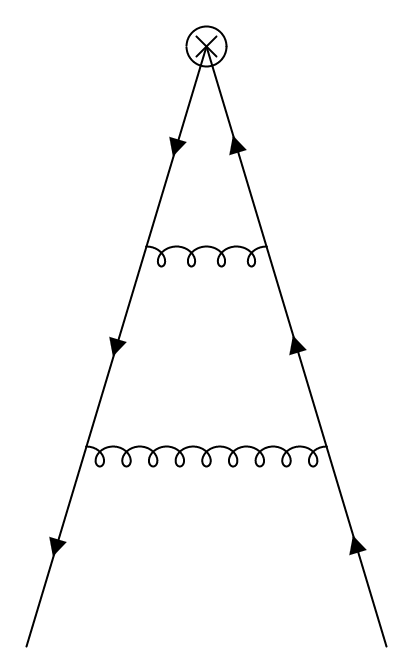
(a) Non-singlet amplitude.
H

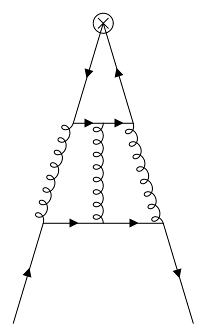
(b) Singlet amplitude induced by a vector current.

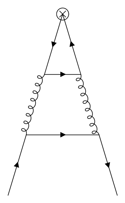
(c) Singlet amplitude induced by an axial-vector current.

Figure 1: Representative Feynman diagrams which contribute to the hard functions. The curly and straight lines denote the gluon and quark propagators, respectively. The crossed circle represents the electroweak current operator.

The Feynman diagrams contributing to the three hard processes under consideration in this paper, off-shell $Z$ or $W^{\pm}$ production, can be grouped into two categories according to whether or not the incident quark lines are connected to the EW vertex or not: the singlet and non-singlet contributions (see Fig. 1). Here, the non-singlet contribution of Fig. 1(a) collects all configurations that connect the external quark lines to the EW vertex while all other configurations are part of the singlet contribution. The latter can be subdivided according to whether they couple to the vector or axial-vector part of the EW vertex, as depicted in Fig. 1(b) and Fig. 1(c), respectively.

$Z$ production.

Here, the quarks coupling to the EW vertex are always of the same flavour. Hence, both singlet and non-singlet amplitudes contribute. In the following, their construction and embedding in the resummation framework is detailed. Their numerical impact is fully examined in App. A. In essence, while at N²LO the impact of the singlet contributions is numerically small, it reaches the same size at N³LO  as the standard non-singlet contribution and it is essential to include it.

All needed amplitudes can in principle be calculated in the full SM and evaluated loop by loop. However, the presence of multiple mass scales complicates the loop integrations considerably, rendering this method somewhat involved. Alternatively, in this work we will employ LEEFT resulting from the SM by integrating out the top quark. For the vector current, due to its conservative nature, the matching from SM onto LEEFT amounts to the re-definitions of the strong coupling $\alpha_{s}$ as well as the field operators [121, 122]. As a results, one can collect the effective vector currents as

$$\begin{split}{V}_{\gamma}^{\mu}=&\;\sum_{q_{i}=u,d,c,s,b}g_{\gamma}^{q_{i}}\,\bar{q}_{i}\gamma^{\mu}q_{i}\,,\\ {V}_{Z}^{\mu}=&\;\sum_{q_{i}=u,d,c,s,b}g_{V}^{q_{i}}\,\bar{q}_{i}\gamma^{\mu}q_{i}\,.\end{split}$$ (2.10)

It is apparent that the expressions for SM light quark vector currents are formally retained in ${V}_{\gamma/Z}^{\mu}$. For later convenience the currents induced by $\gamma^{*}q\bar{q}$ and $Z^{*}q\bar{q}$ vertices are listed separately. In absence of the EW corrections, one can always distinguish them. The coupling factors $g_{\gamma,V}^{q_{i}}$ collect the EW coupling constants,

$$\begin{split}g_{\gamma}^{q}=&\;e\,Q_{q}\;,\hskip 28.45274pt{}g_{V}^{q}=\frac{e}{s_{w}\,c_{w}}\left(\frac{T^{3}_{q}}{2}\,-Q_{q}\,s_{w}^{2}\right)\,.\end{split}$$ (2.11)

Here we utilise $e$ as the electromagnetic coupling and $s_{w}$ and $c_{w}$ as the sine and cosine of the weak-mixing angle $\theta_{w}$. $T^{3}_{q}$ and $Q_{q}$ are the third component of the weak isospin and charge for the quark $q$, respectively.

The axial-vector current on the other hand, which exists only for $Z$ boson exchange, requires a more delicate matching procedure. As the renormalisability of SM relies on the anomaly cancellation within each quark generation, the removal of the top quark by brute force will break the renormalisation group invariance (RGI) explicitly and thus it necessitates an additional renormalisation constant in the LEEFT for its restoration. To this end, the following operator basis is proposed for the axial-vector effective current [123, 124, 125, 126],

$$\begin{split}A_{Z}^{\mu}=&\;g_{A}\left[\sum_{i=1,2,3}\Delta_{i}^{\mathrm{ns}}+C_{t}\mathcal{O}_{s}\right]\;,\end{split}$$ (2.12)

where the coupling factor $g_{A}$ again collects the EW coupling constant, i.e.

$$\begin{split}g_{A}=&\;-\frac{e}{4\,s_{w}\,c_{w}}\;.\end{split}$$ (2.13)

It is independent of the quark flavour. $\Delta_{i}^{\mathrm{ns}}$ stands for the non-singlet operators of the $i$th quark generation,

$$\begin{split}\Delta^{\mathrm{ns}}_{1}=\bar{u}\gamma^{\mu}\gamma_{5}u-\bar{d}\gamma^{\mu}\gamma_{5}d,\,~{}~{}\,\Delta^{\mathrm{ns}}_{2}=\bar{c}\gamma^{\mu}\gamma_{5}c-\bar{s}\gamma^{\mu}\gamma_{5}s,\,~{}~{}\,\Delta^{\mathrm{ns}}_{3}=\frac{\mathcal{O}_{s}}{N_{F}}-\bar{b}\gamma^{\mu}\gamma_{5}b\;.\end{split}$$ (2.14)

For the first two quark generations, the operators $\Delta^{\mathrm{ns}}_{1,2}$ are formally identical to those in SM, whilst for the third one, $\Delta^{\mathrm{ns}}_{3}$ is artificially constructed to facilitate the anomalous cancellation. Here $N_{F}$ represents the number of massless quarks, taking the value $N_{F}=5$ throughout this work. $\mathcal{O}_{s}$ is the singlet operator, which is defined as

$$\begin{split}\mathcal{O}_{s}=\sum_{q_{i}=u,d,c,s,b}\bar{q}_{i}\gamma^{\mu}\gamma_{5}q_{i}.\end{split}$$ (2.15)

In addition, $A_{Z}^{\mu}$ also comprises a novel structure $C_{t}\mathcal{O}_{s}$ beyond what is present in the SM. In presence of the axial-anomaly, the renormalised singlet $\mathcal{O}_{s}$ operator exhibits the explicit dependence on the renormalisation group transformations (RGT). However, this RGT-dependence will be eliminated order by order by the Wilson coefficient $C_{t}$ such that the RGI is still maintained in LEEFT. To calculate $C_{t}$, one needs to compare the SM amplitudes induced by $\bar{t}\gamma^{\mu}\gamma_{5}t-\bar{b}\gamma^{\mu}\gamma_{5}b$ with those from $\mathcal{O}_{s}$ in the limit $M_{L}\ll m_{t}$. Here $m_{t}$ denotes the pole mass of the top quark. In this work we follow the conventions of [125],

$$\begin{split}C_{t}=&\;-\frac{1}{N_{F}}+\left(\frac{\alpha_{s}}{4\pi}\right)^{2}\left(-8L_{t}+4\vphantom{\frac{\pi^{2}}{6}}\right)+\left(\frac{\alpha_{s}}{4\pi}\right)^{3}\left(-\frac{184}{3}L_{t}^{2}-\frac{784}{9}L_{t}+208\zeta_{3}-\frac{6722}{27}\right)\;.\end{split}$$ (2.16)

where $L_{t}=\ln(\mu^{2}/m_{t}^{2})$. Here the tree-level result $(-1/N_{F})$ balances the $\mathcal{O}_{s}/N_{F}$ term in $\Delta^{\mathrm{ns}}_{3}$. The singlet contribution starts from the two-loop level and the $\mathcal{O}(\alpha^{2}_{s})$ results can be either straightforwardly read from the axial-anomaly form factor in Ref. [135], or extracted from [136, 124]. The third order expressions can be found in Ref. [123]. Particular attention needs to be noted that in Refs. [123, 124] the $\mathcal{O}_{s}$ operator is renormalised in a different prescription from those in Refs. [125, 135]. Their conversion is essential and we present the corresponding details in App. C.

Now that we have all ingredients at hand we can finally calculate the hard function. From eq. (2.9), the hard sector can be addressed from the square of IRC-subtracted on-shell amplitudes. In absence of EW corrections, the amplitudes involved can be naturally decomposed into two parts: the hadronic and the leptonic currents. The hadronic current can be expressed using the effective vector and axial-vector currents, $V_{Z/\gamma}^{\mu}$ and $A_{Z}^{\mu}$, respectively. More explicitly, we have

$$\begin{split}H^{\mu,ij}_{\gamma}=&\;\sqrt{\mathcal{Z}_{\mathcal{B}_{+}}\mathcal{Z}_{\mathcal{B}_{-}}\mathcal{Z}_{\mathcal{S}}}\,\langle 0|V_{\gamma}^{\mu}|q_{i}\bar{q}_{j}\rangle=\left(g_{\gamma}^{q_{i}}C_{\mathrm{ns}}+g_{\gamma}^{\scriptscriptstyle\Sigma}C_{\mathrm{s}}^{V}\right)\mathcal{V}^{\mu}_{ij}\,,\\ H^{\mu,ij}_{Z,V}=&\;\sqrt{\mathcal{Z}_{\mathcal{B}_{+}}\mathcal{Z}_{\mathcal{B}_{-}}\mathcal{Z}_{\mathcal{S}}}\,\langle 0|V_{Z}^{\mu}|q_{i}\bar{q}_{j}\rangle=\left(g_{V}^{q_{i}}C_{\mathrm{ns}}+g_{V}^{\scriptscriptstyle\Sigma}C_{\mathrm{s}}^{V}\right)\mathcal{V}^{\mu}_{ij}\,,\\ H^{\mu,ij}_{Z,A}=&\;\sqrt{\mathcal{Z}_{\mathcal{B}_{+}}\mathcal{Z}_{\mathcal{B}_{-}}\mathcal{Z}_{\mathcal{S}}}\,\langle 0|A_{Z}^{\mu}|q_{i}\bar{q}_{j}\rangle=g_{A}\left[\left(2T_{q_{i}}+\frac{1}{N_{F}}\right)C_{\mathrm{ns}}+C_{t}C_{\mathrm{s}}^{A}\right]\mathcal{A}^{\mu}_{ij}\,,\end{split}$$ (2.17)

where $g_{\gamma/V}^{\scriptscriptstyle\Sigma}$ is introduced to collect the EW coupling, namely,

$$\begin{split}g_{\gamma}^{\scriptscriptstyle\Sigma}\equiv\sum_{q_{i}=u,d,s,c,b}g^{q_{i}}_{\gamma}\;,\hskip 28.45274ptg_{V}^{\scriptscriptstyle\Sigma}\equiv\sum_{q_{i}=u,d,s,c,b}g^{q_{i}}_{V}\;.\end{split}$$ (2.18)

$\mathcal{V}^{\mu}_{ij}$ and $\mathcal{A}^{\mu}_{ij}$ are born level amplitudes induced by the vector and axial-vector vertices, respectively. Their expressions read,

$$\begin{split}\mathcal{V}^{\mu}_{ij}=\delta_{ij}\,\langle 0|\bar{q_{i}}\gamma^{\mu}q_{i}|q_{i}\bar{q}_{i}\rangle\Big{|}_{\mathrm{Born}}\,,\hskip 28.45274pt\mathcal{A}^{\mu}_{ij}=\delta_{ij}\,\langle 0|\bar{q_{i}}\gamma^{\mu}\gamma_{5}q_{i}|q_{i}\bar{q}_{i}\rangle\Big{|}_{\mathrm{Born}}\,.\end{split}$$ (2.19)

As the massless QCD interactions conserve chirality, one can always factor them out after the renormalisation and IRC-pole subtraction. In addition, we have also utilised a set of hard coefficients in eq. (2.17) encoding the loop corrections. $C_{\text{ns}}$ contains all the non-singlet contributions (see Fig. 1(a)) and can be extracted from the $\gamma^{*}q\bar{q}$ form factor. In the recent years, the $\gamma^{*}q\bar{q}$ form factor has been calculated up to three-loop level [137, 138, 114]. Further, $C_{\text{s}}^{V}$ stems from the singlet contribution to the vector current (see Fig. 1(b)). As Furry’s theorem forbids contributions at two-loop order, the lowest order result enters at $\mathcal{O}(\alpha_{s}^{3})$, see [138, 114]. Similarly, $C_{\text{s}}^{A}$ represents the QCD corrections induced by $\mathcal{O}_{s}$. Its N²LO expression can be extracted from Refs. [137, 138, 114, 135], while the logarithmic dependences at third-loop order accuracy can be obtained from the anomalous dimensions. The specific expressions for all three coefficient functions $C_{\text{ns}}$, $C_{\text{s}}^{V}$ and $C_{\text{s}}^{A}$ are listed in App. C.

Besides the hadronic contributions, the hard function also comprises the leptonic ones, namely the leptonic currents, including the vector boson propagators,

$$\begin{split}L^{\mu}_{\gamma}=&\;\frac{g_{\gamma}^{\ell}}{M^{2}_{L}}\;\langle\ell^{+}\ell^{-}|\bar{\ell}\gamma^{\mu}\ell|0\rangle\,,\\ L_{Z,V}^{\mu}=&\;\frac{g_{V}^{\ell}}{M_{L}^{2}-\mu_{Z}^{2}}\;\langle\ell^{+}\ell^{-}|\bar{\ell}\gamma^{\mu}\ell|0\rangle\,,\\ L_{Z,A}^{\mu}=&\;\frac{g_{A}^{\ell}}{M_{L}^{2}-\mu_{Z}^{2}}\;\langle\ell^{+}\ell^{-}|\bar{\ell}\gamma^{\mu}\gamma_{5}\ell|0\rangle\;.\end{split}$$ (2.20)

Therein, $\mu_{Z}$ stands for the complex mass of $Z$ boson, which will be introduced properly in Sec. 3.1. In absence of EW corrections, the couplings of the leptonic sector $g_{\gamma,V,A}^{\ell}$ can be inferred from the leading order vertices,

$$\begin{split}g_{\gamma}^{\ell}=e\,Q_{\ell}\,,\qquad g_{V}^{\ell}=\frac{e}{s_{w}\,c_{w}}\left[\frac{T^{3}_{\ell}}{2}-Q_{\ell}\,s_{w}^{2}\right]\,,\qquad\text{and}\qquad g_{A}^{\ell}=-\frac{e}{\,s_{w}\,c_{w}}\cdot\frac{T^{3}_{\ell}}{2}\;.\end{split}$$ (2.21)

Putting all pieces together, the hard function can be expressed as

$$\begin{split}\mathcal{H}^{\gamma/Z}_{ij}(m_{t},M_{L},\Omega_{L},\mu)=&\;\overline{\sum_{\mathrm{col,pol}}}\,\left|H^{\mu,ij}_{\gamma}L_{\gamma,\mu}+\left(H^{\mu,ij}_{Z,V}+H^{\mu,ij}_{Z,A}\right)\left(L_{Z,V,\mu}+L_{Z,A,\mu}\vphantom{H^{j}_{Z}}\right)\right|^{2}\;.\end{split}$$ (2.22)

$W^{\pm}$ production.

In this process, as the quarks participating in the EW vertex are always of different flavours, only non-singlet diagrams will contribute. In analogy to eqs. (2.17)-(2.22), we write the hard functions as

$$\begin{split}\mathcal{H}^{W}_{ij}(M_{L},\Omega_{L},\mu)=&\;\overline{\sum_{\mathrm{col,pol}}}\,\big{|}H^{\mu,ij}_{W}L_{W,\mu}\big{|}^{2}\;,\end{split}$$ (2.23)

where

$$\begin{split}H^{\mu,ij}_{W}=&\frac{e\,V_{ji}}{2\sqrt{2}\,s_{w}}\,C_{\text{ns}}\,\langle 0|\bar{q_{j}}\gamma^{\mu}(1-\gamma_{5})q_{i}|q_{i}\bar{q}_{j}\rangle\Big{|}_{\mathrm{Born}}\,,\\ L_{W}^{\mu}=&\frac{e}{2\sqrt{2}\,s_{w}}\frac{1}{M^{2}_{L}-\mu_{W}^{2}}\;\langle\ell^{\pm}\nu(\bar{\nu})|\bar{\ell}\gamma^{\mu}(1-\gamma_{5})\ell|0\rangle\,.\\ \end{split}$$ (2.24)

Here $V_{ji}$ signals the Cabibbo-Kobayashi-Maskawa (CKM) matrix, and $\mu_{W}$ represents the complex mass of the $W$ boson.

2.3 Resummation

With the help of eq. (2.4), the scales relevant to the small $q_{\mathrm{T}}$ regime can be successfully separated. However, in presence of the scale hierarchy, such as $q_{\mathrm{T}}\ll M_{L}$, any fixed-order expansion of eq. (2.4) will suffer from the large logarithmic terms reducing the perturbativity. To address this issue, we employ the solutions of RGEs as well as the rapidity group equations (RaGEs) to carry out the scale evolution. In this way, the fixed-order functions contribute only at their intrinsic scales and the large logarithmic terms arising from the scale hierarchy can collectively be resummed within the exponential functions of the evolution. The procedure is detailed in the following.

We begin with the RGEs and RaGEs for each sector. The RGE for $C_{t}$ reads

$$\begin{split}\frac{{\rm d}}{{\rm d}\ln\mu^{2}}\ln C_{t}(m_{t},\mu)=-\gamma_{t}\;,\end{split}$$ (2.25)

where $\gamma_{t}$ is the anomalous dimension and its N³LO result can be found in Ref. [125]. The evolution equations for $C_{\text{ns}}$, $C_{\text{s}}^{A}$ and $C_{\text{s}}^{V}$ can be expressed as

$$\begin{split}\frac{{\rm d}}{{\rm d}\ln\mu^{2}}\ln C_{\text{ns}}(M_{L},\mu)=&\;\frac{\Gamma_{\mathrm{cusp}}}{2}\,\ln\bigg{[}\frac{-M_{L}^{2}-i\epsilon}{\mu^{2}}\bigg{]}+\gamma_{h}\;,\\ \frac{{\rm d}}{{\rm d}\ln\mu^{2}}\ln C_{\text{s}}^{A}(M_{L},\mu)=&\;\frac{\Gamma_{\mathrm{cusp}}}{2}\,\ln\bigg{[}\frac{-M_{L}^{2}-i\epsilon}{\mu^{2}}\bigg{]}+\gamma_{h}+\gamma_{t}\;,\\ \frac{{\rm d}}{{\rm d}\ln\mu^{2}}\ln C_{\text{s}}^{V}(M_{L},\mu)=&\;\frac{\Gamma_{\mathrm{cusp}}}{2}\,\ln\bigg{[}\frac{-M_{L}^{2}-i\epsilon}{\mu^{2}}\bigg{]}+\gamma_{h}\;,\end{split}$$ (2.26)

where $\Gamma_{\mathrm{cusp}}$ stands for the cusp anomalous dimension. Its result is known at the three-loop accuracy [139], whilst the four-loop evaluation has been accomplished very recently [113]. $\gamma_{h}$ represents the hard anomalous dimensions and can be extracted from [114]. The remaining equations for the soft and beam functions, $\mathcal{S}$ and $\mathcal{B}$, read [101]

$$\begin{split}\frac{\partial}{\partial\ln\mu^{2}}\ln\mathcal{S}(\vec{b}_{\mathrm{T}},\mu,\nu)=&\;\Gamma_{\mathrm{cusp}}\,\ln\bigg{[}\frac{\mu^{2}}{\nu^{2}}\bigg{]}-\gamma_{s}\;,\\ \frac{\partial}{\partial\ln\mu^{2}}\ln\mathcal{B}(\eta,\vec{b}_{\mathrm{T}},\mu,\nu)=&\;\Gamma_{\mathrm{cusp}}\,\ln\bigg{[}\frac{\nu}{\eta\sqrt{s}}\bigg{]}+\gamma_{b}\;,\end{split}$$ (2.27)

and

$$\begin{split}\frac{\partial}{\partial\ln\nu^{2}}\ln\mathcal{S}(\vec{b}_{\mathrm{T}},\mu,\nu)=&\;-2\,\frac{\partial}{\partial\ln\nu^{2}}\ln\mathcal{B}(\eta,\vec{b}_{\mathrm{T}},\mu,\nu)=\gamma_{r}\left[\alpha_{s}\left(\frac{b_{0}}{b_{\mathrm{T}}}\right)\right]+\int_{\mu^{2}}^{\frac{b_{0}^{2}}{b_{\mathrm{T}}^{2}}}\frac{{\rm d}\bar{\mu}^{2}}{\bar{\mu}^{2}}\;\Gamma_{\mathrm{cusp}}\left[\alpha_{s}(\bar{\mu})\right]\;.\end{split}$$ (2.28)

Therein, $\gamma_{s}$ is the soft anomalous dimension, on which the accuracy has already arrived at N³LO [115]. $\gamma_{b}$ is the non-cusp anomalous dimension for the beam function, which can be derived from the consistency relationship $\gamma_{b}=(\gamma_{s}-2\gamma_{h})/2$. In addition to the ingredients of the RGEs, the rapidity anomalous dimension, $\gamma_{r}$, is involved within the RaGEs. Its universality (or the rapidity regulator independence) has been discussed in Refs. [140, 101], and the N³LO results are detailed in Refs. [102, 140].

Logarithmic accuracy$\int_{A}^{B}$	$C_{\text{ns}}$, $C_{\text{s}}^{A}$, $C_{\text{s}}^{V}$, $C_{t}$, $\mathcal{S}$, $\mathcal{B}$	$\Gamma_{\text{cusp}}$	$\gamma_{t,h,s,b}$
NLL′$\int_{A}^{B}$	$\mathcal{O}(\alpha_{s})$	$\mathcal{O}(\alpha^{2}_{s})$	$\mathcal{O}(\alpha_{s})$
N2LL′$\int_{A}^{B}$	$\mathcal{O}(\alpha^{2}_{s})$	$\mathcal{O}(\alpha^{3}_{s})$	$\mathcal{O}(\alpha^{2}_{s})$
N3LL′$\int_{A}^{B}$	$\mathcal{O}(\alpha^{3}_{s})$	$\mathcal{O}(\alpha^{4}_{s})$	$\mathcal{O}(\alpha^{3}_{s})$

Table 1: Needed accuracy of the fixed-order inputs to achieve a given logarithmic accuracy of the resummation, in accordance with eq. (1.1).

With all ingredients collected, we can now carry out the resummation. In this work, the resummed distributions are calculated at NLL^′, N²LL^′, and N³LL^′ level. For each level of the logarithmic accuracy, the perturbative order for each ingredient can be found out in eq. (1.1) and has been also summarised in Tab. 1. Note that as the accuracy of the fixed-order functions is counted with respect to Born cross section, only the $\mathcal{O}(\alpha_{s}^{3})$ terms for $C_{\text{s}}^{V}$ are needed in this paper. The resummed spectrum is then obtained by substituting the solutions of the RGEs as well as RaGEs into eq. (2.4), giving

$$\begin{split}\frac{{\rm d}^{4}\sigma_{\text{res}}}{{\rm d}^{2}\vec{q}_{\mathrm{T}}\,{\rm d}Y_{L}\,{\rm d}M_{L}^{2}\,{\rm d}\Omega_{L}}=&\;\frac{1}{16s(2\pi)^{4}M_{L}^{2}}\;\sum_{i,j}\int{\rm d}^{2}\vec{b}_{\mathrm{T}}\;e^{i\vec{b}_{\mathrm{T}}\cdot\vec{q}_{\mathrm{T}}}\;\mathcal{U}_{V}(\mu_{h},\mu_{b_{\pm}},\mu_{s},\nu_{b_{\pm}})\;\mathcal{U}_{R}(\mu_{s},\nu_{b_{\pm}},\nu_{s})\\ &\hskip 142.26378pt\times\vphantom{\sum_{i,j}}\widetilde{\mathcal{H}}^{V,\mathrm{res}}_{ij}(M_{L},\Omega_{L},\mu_{h})\;\mathcal{S}({\vec{b}_{T}},\mu_{s},\nu_{s})\\ &\hskip 142.26378pt\times\mathcal{B}_{+}^{i}(\eta_{+},\vec{b}_{T},\mu_{b_{+}},\nu_{b_{+}})\;\mathcal{B}_{-}^{j}(\eta_{-},\vec{b}_{T},\mu_{b_{-}},\nu_{b_{-}})\;,\end{split}$$ (2.29)

where the kernels $\mathcal{U}_{V,R}$, respectively, effect the virtuality and rapidity evolutions. Their explicit expressions read

$$\begin{split}\mathcal{U}_{V}&=\;\exp\bigg{\{}\int_{\mu^{2}_{h}}^{\mu^{2}_{b_{\pm}}}\frac{{\rm d}\bar{\mu}^{2}}{\bar{\mu}^{2}}\Big{[}-\Gamma_{\mathrm{cusp}}\ln\left(\frac{\bar{\mu}^{2}}{M_{L}^{2}}\right)+2\gamma_{h}\Big{]}+\int_{\mu^{2}_{s}}^{\mu^{2}_{b_{\pm}}}\frac{{\rm d}\bar{\mu}^{2}}{\bar{\mu}^{2}}\Big{[}\Gamma_{\mathrm{cusp}}\ln\left(\frac{\bar{\mu}^{2}}{\nu^{2}_{b_{\pm}}}\right)-\gamma_{s}\Big{]}\bigg{\}}\,,\\ \mathcal{U}_{R}&=\;\exp\bigg{\{}\ln\left[\frac{\nu^{2}_{b_{\pm}}}{\nu^{2}_{s}}\right]\Bigg{[}\gamma_{r}\left(\alpha_{s}\left(\frac{b_{0}}{b_{\mathrm{T}}}\right)\right)+\int^{\frac{b^{2}_{0}}{b_{\mathrm{T}}^{2}}}_{\mu^{2}_{s}}\frac{{\rm d}\bar{\mu}^{2}}{\bar{\mu}^{2}}\;\Gamma_{\mathrm{cusp}}\left[\alpha_{s}(\bar{\mu})\right]\Bigg{]}\bigg{\}}\,.\end{split}$$ (2.30)

Finally, $\widetilde{\mathcal{H}}^{V,\mathrm{res}}_{ij}$ is the part of the hard function participating in the resummation. In $W^{\pm}$ production, as $M_{L}$ is the only physical scale in the hard sector, the natural choice of scale $\mu_{h}$ can be easily identified (assuming it is related to $M_{L}$). $\widetilde{\mathcal{H}}^{V,\mathrm{res}}_{ij}$ then coincides directly with $\mathcal{H}^{W}_{ij}$ from eq. (2.23), giving

$$\begin{split}\widetilde{\mathcal{H}}^{W,\mathrm{res}}_{ij}(M_{L},\Omega_{L},\mu_{h})=\mathcal{H}^{W}_{ij}(M_{L},\Omega_{L},\mu_{h})\;.\end{split}$$ (2.31)

Conversely, the hard function in $Z$ production, contains a second intrinsic scale in addition to $M_{L}$, $m_{t}$, originating in the singlet contributions. In order to resum the logarithm associated with their scale hierarchy, $\ln[m^{2}_{t}/M^{2}_{L}]$, we substitute the Wilson coefficient $C_{t}$ in eq. (2.11) with its resummed version,

$$\begin{split}C_{t}^{\mathrm{res}}(m_{t},\mu_{h})=&\;C_{t}(m_{t},\mu_{t})\,\exp\left[-\int_{\mu^{2}_{t}}^{\mu^{2}_{h}}\frac{d\mu^{2}}{\mu^{2}}\,\gamma_{t}\right]\;,\end{split}$$ (2.32)

and then evaluate all other Wilson coefficients $C_{\text{ns}}$, $C_{\text{s}}^{V}$ and $C_{\text{s}}^{A}$, at the scale ${\mu_{h}}$. As a result, the part of the hard function participating in the resummation can be expressed as

$$\begin{split}\widetilde{\mathcal{H}}^{\gamma/Z,\mathrm{res}}_{ij}(m_{t},M_{L},\Omega_{L},\mu_{h})=&\;\mathcal{H}^{\gamma/Z}_{ij}\Bigg{|}_{\genfrac{}{}{0.0pt}{3}{C_{t}\to C_{t}^{\mathrm{res}}(m_{t},\mu_{h}),C_{\text{ns}}\to C_{\text{ns}}(M_{L},\mu_{h})}{C_{\text{s}}^{V}\to C_{\text{s}}^{V}(M_{L},\mu_{h}),C_{\text{s}}^{A}\to C_{\text{s}}^{A}(M_{L},\mu_{h})}}\;.\end{split}$$ (2.33)

2.4 Power corrections

To extrapolate eq. (2.29) to the entire phase space, it is crucial to properly account for power corrections stemming from the truncation of the asymptotic series in $q_{\mathrm{T}}/{M_{L}}$ (recalling that eq. (2.4) only contains the leading power contributions). They can impact both the leptonic currents $L_{W,Z,\gamma}^{\mu}$ (in eq. (2.20) and eq. (2.24)) as well as the hadronic ones. To improve the lepton currents, we substitute the $L_{W,Z,\gamma}^{\mu}$ by their pre-expanded results, i.e.

$$\begin{split}L_{V}^{\mu}\longrightarrow\Lambda^{\mu}_{\ell,\nu}(\vec{q}_{\mathrm{T}})L_{V}^{\nu}\;,\end{split}$$ (2.34)

where $V=W,Z,\gamma$. $\Lambda^{\mu}_{\ell,\nu}$ accounts for the Lorentz transformation from the leptonic centre of mass reference frame to the rest frame of the initial proton pair or lab frame. Noting that in eq. (2.20) and eq. (2.24), as a result of the $q_{\mathrm{T}}/M_{L}$ expansion in the hard sector, $L_{V}^{\mu}$ is defined in the lepton centre of mass frame. Thus, the replacement in eq. (2.34) restores the leptonic currents to their form in the exact SM calculation. Their impact is assessed in App. B. It is worth noting that even though the substitution in eq. (2.34) manifestly breaks energy-momentum conservation when coupling the hadronic and the corrected leptonic tensor, it induces no gauge violations in practice. This is because the longitudinal component of the $\gamma$, $Z$, or $W^{\pm}$ propagators can always be eliminated by the attached leptonic currents in the massless limit. Alternative methods with the analogous effects can also be found in Refs. [141, 142, 143, 108, 119]. Very recently, a systematic classification has been carried out in Ref. [112] as to the leptonic power corrections.

On the other hand, it is also necessary to handle the power corrections to the hadronic currents. In principle, one can incorporate them power by power with the aid of the subleading SCET Lagrangians and Hamiltonians [130, 95, 144]. Nevertheless, not only can more structures beyond eq. (2.4) be introduced by the subleading vertices, the inhomogeneity in asymptotic series, which arises from the rapidity regulation, may further complicate the investigations [145, 146, 147]. So for simplicity, this work only considers the leading power factorisation and the according resummation in the hadronic sector, treating the power corrections through the matching to fixed-order.

2.5 Matching to fixed-order QCD and observable calculation

Finally, we match the resummation to the exact QCD fixed-order calculation. We therefore introduce the following matching procedure,

$$\begin{split}\frac{{\rm d}\sigma_{\text{mat}}}{{\rm d}\Phi}=&\;\left\{\frac{{\rm d}\sigma_{\text{res+lpc}}}{{\rm d}\Phi}-\frac{{\rm d}\sigma_{\text{exp+lpc}}}{{\rm d}\Phi}(\mu_{R},\mu_{F})\right\}f\left(\frac{q_{\mathrm{T}}}{\mu_{Q}}\right)+\frac{{\rm d}\sigma_{\text{f.o.}}}{{\rm d}\Phi}(\mu_{R},\mu_{F})\;,\end{split}$$ (2.35)

where $\sigma_{\text{exp+lpc}}$ is the fixed-order expansion of $\sigma_{\text{res+lpc}}$ and the “lpc” addition in the subscript signals the inclusion of the leptonic power corrections. $\sigma_{\text{f.o.}}$ denotes the exact fixed-order perturbative result at the conventional renormalisation and factorisation scales $\mu_{R}$ and $\mu_{F}$. Of course, both $\sigma_{\text{exp+lpc}}$ and $\sigma_{\text{f.o.}}$ must be expanded to the same order. ${\rm d}\Phi$ stands for the differential phase space element ${\rm d}^{2}\vec{q}_{\mathrm{T}}\,{\rm d}Y_{L}\,{\rm d}M_{L}^{2}\,{\rm d}\Omega_{L}$. The transition function $f$ is introduced to assure that the resummation is only active in the asymptotic region, more explicitly,

$$\begin{split}f\left(\frac{q_{\mathrm{T}}}{\mu_{Q}}\right)=\frac{1}{1+a^{\frac{q_{\mathrm{T}}}{\mu_{Q}}-1}}\hskip 93.89265pt\begin{minipage}{225.34381pt} \includegraphics{text/Diag/fx.pdf} \end{minipage}\end{split}$$ (2.36)

The numerical choice of the matching scale $\mu_{Q}$ will be discussed in Sec. 3. The base of the exponent $a$ can be thought of as a free parameter governing the shape of the transition function. We choose to link it to $\mu_{Q}$ and define it as $a=\exp(\mu_{Q}/q_{\mathrm{T}}^{\text{ref}})$, $q_{\mathrm{T}}^{\text{ref}}$ is taken to be 1 GeV. It is important to note that although $f$ is smaller than unity for all physical $q_{\mathrm{T}}$, the precise choice of $\mu_{Q}$ will ensure that it differs from unity by amounts much smaller than one permille in a wide region around the Sudakov peak where the resummation effects dominate. Likewise, $q_{\mathrm{T}}=\mu_{Q}$ does not mark the endpoint of the resummation region, but where the resummation effects are faded out to half their intrinsic size, $f(1)=\tfrac{1}{2}$. The functional form then induces a symmetric reduction of the influence of the resummation in the region $[\mu_{Q}-\Delta q_{\mathrm{T}},\mu_{Q}+\Delta q_{\mathrm{T}}]$, wherein $\Delta q_{\mathrm{T}}=q_{\mathrm{T}}^{\text{ref}}\ln((1-f)/f)$ and $f$ is the fraction of reduction. Thus, with the above value for $q_{\mathrm{T}}^{\text{ref}}$ the resummation effects are reduced from 99% to 1% of their actual size in the interval $\mu_{Q}\mp 4.6\,\text{GeV}$. The functional form of the base of the exponent $a$ ensures that the width of the transition region, $\Delta q_{\mathrm{T}}$, is directly proportional to $q_{\mathrm{T}}^{\text{ref}}$, with $q_{\mathrm{T}}^{\text{ref}}$ taking the role of an easily interpretable shape parameter.

When $\vec{q}_{\mathrm{T}}$ enters the hadronic regime $\Lambda_{\mathrm{QCD}}\sim q_{\mathrm{T}}\ll M_{L}$, the non-perturbative contributions become non-negligible. Hence, a modification factor parametrising the non-perturbative dynamics of this regime, $S_{\mathrm{mod}}(b_{\mathrm{T}}^{2})$, encoding all the hadronic contributions within the low $q_{\mathrm{T}}$ region [148, 149], should be introduced. In the recent years, a number of parametrisations and input extractions of $S_{\mathrm{mod}}(b_{\mathrm{T}}^{2})$ have been discussed in the literatures [150, 151, 152, 16, 153, 15, 154]. However, as the main concern of this work is with the perturbative domain, we ignore $S_{\mathrm{mod}}(b_{\mathrm{T}}^{2})$ here and leave its incorporation to the future investigations.

Taking the integral of eq. (2.35) together with the customised theta and delta functions, one is able to implement the fiducial cuts and carry out the observable calculations, more explicitly,

$$\begin{split}\frac{{\rm d}\sigma}{{\rm d}O}=&\;\int{\rm d}\Phi\;\Theta\Big{[}\mathcal{G}\big{(}\Phi\big{)}\Big{]}\;\delta\Big{[}O-\mathcal{F}_{O}\big{(}\Phi\big{)}\Big{]}\;\frac{{\rm d}\sigma_{\mathrm{mat}}}{{\rm d}\Phi},\end{split}$$ (2.37)

where $\mathcal{G}$ is a function of the phase space encoding the fiducial cuts. $O$ stands for a generic observable and $\mathcal{F}_{O}$ is its corresponding functional definition. This work focusses on the $q_{\mathrm{T}}$ and $\Delta\phi$ spectra, giving

$$\begin{split}\mathcal{F}_{q_{\mathrm{T}}}=&\;|\vec{q}_{\mathrm{T}}|,\\ \mathcal{F}_{\Delta\phi}=&\;\arccos\left[\frac{\vec{p}_{{}_{1,\mathrm{T}}}\cdot\vec{p}_{{}_{2,\mathrm{T}}}}{|\vec{p}_{{}_{1,\mathrm{T}}}||\vec{p}_{{}_{2,\mathrm{T}}}|}\right].\end{split}$$ (2.38)

Here $\vec{p}_{{}_{1(2),\mathrm{T}}}$ denotes the transverse momentum of the final (anti-)lepton in the lab frame. In particular, both variables are purely transverse and are thus well-defined for both $W$ and $Z$ production in a realistic detector environment where only the transverse part of the neutrino’s momentum is observable through as missing transverse momentum. Further, in calculating the phase-space integral of eq. (2.37), we retain the full kinematic dependences in $\mathcal{G}(\Phi)$ and $\mathcal{F}_{O}(\Phi)$ and do not carry out any multipole-expansions.

3 Numerical Results

In this section we are discussing numerical results obtained with the methods outlined in the previous section for a representative fiducial region.

3.1 Setup and fiducial region

Throughout this paper, all distributions for $W^{\pm}$ production are calculated in the $G_{\mu}$ scheme while those for $Z$ production are calculated in the $\alpha(m_{Z})$ scheme. We use the following input parameters [155]

$G_{\mu}$	​​=​​	$1.166378\times 10^{-5}\,\text{GeV}^{-2}$
$m_{W}$	​​=​​	80.379 GeV	$\Gamma_{W}$	​​=​​	2.085 GeV
$m_{Z}$	​​=​​	91.1876 GeV	$\Gamma_{Z}$	​​=​​	2.4955 GeV
$m_{t}$	​​=​​	173.2 GeV .

The width of the top quark as well as the mass and the width of the Higgs boson have no phenomenological impact and are neglected. All other particles are considered massless. We work in the complex-mass scheme [156], with the complex masses and mixing angles defined through

$$\mu_{i}^{2}=m_{i}^{2}-\mathrm{i}m_{i}\Gamma_{i}\qquad\text{and}\qquad\sin^{2}\theta_{w}=1-\frac{\mu_{W}^{2}}{\mu_{Z}^{2}}\;.$$ (3.1)

The electromagnetic coupling constant is defined as

$$\alpha_{G_{\mu}}=\left|\frac{\sqrt{2}G_{\mu}\mu_{W}^{2}\sin^{2}\theta_{w}}{\pi}\right|\qquad\text{and}\qquad\alpha_{m_{Z}}=1/128.802$$ (3.2)

in the $G_{\mu}$ and $\alpha(m_{Z})$ schemes, respectively. Other input schemes, in particular for $Z$ boson production, may be chosen in order to improve the description of the correlations of the lepton pair system and the hadronic recoil, e.g. by using the weak mixing angle as an input parameter [157]. Furthermore, we use the NNPDF31_nnlo_as_0118 [13] parton distribution functions, interfaced through L HAPDF [158], with the corresponding value of the strong coupling $\alpha_{s}(m_{Z})=0.118$. In accordance with this choice we neglect all photon induced contributions. The CKM matrix is chosen as diagonal, i.e. $V_{ij}=\delta_{ij}$.

To carry out the resummation entering our matched results of eqs. (2.35) and (2.37), we employ the C UBA library [159, 160] performing the respective integrations and make use of L HAPDF evolving the factorisation scale. To tackle the harmonic poly-logarithms participating in the $\mathcal{I}_{ij}$ function (see eq. (2.8)), the package HPOLY [161] is used. The LO hard functions in eqs. (2.23) and (2.22) are computed with FeynCalc [162, 163, 164] and FeynArts [165, 166]. All remaining parts of the hard function, in particular the non-singlet and singlet contributions $C_{\text{ns}}$, $C_{\text{s}}^{V}$, and $C_{\text{s}}^{A}$ as well as the top-quark contribution $C_{t}$, are implemented analytically. The fixed-order contribution to eq. (2.35) and, hence, the matched result is computed using S HERPA [167, 168] in combination with O PEN L OOPS [169, 170]. In this framework, renormalised virtual amplitudes are provided by O PEN L OOPS , which uses C OLLIER tensor reduction library [171] as well as C UT T OOLS [172] together with the O NE L OOP library [173]. All remaining tasks, i.e. the bookkeeping of partonic subprocesses, phase-space integration, and the subtraction of all infrared singularities, are provided by S HERPA using the matrix element generator A MEGIC [174, 175, 176].

In estimating the theoretical uncertainties, we emphasise two aspects. The first one is the uncertainty arising from higher order corrections, which can be estimated by examining the sensitivity of the results to the scale variations. As presented in Sec. 2.5 the matched result depends on a set of auxiliary scales, originating both in the resummation and the fixed-order calculation, $\{\mu,\nu\}\equiv\{\mu_{t},\mu_{h},\mu_{b_{+}},\mu_{b_{-}},\mu_{s},\nu_{b_{+}},\nu_{b_{-}},\mu_{R},\mu_{F}\}$. During the numerical implementation, we take $\mu_{b}=\mu_{b_{\pm}}$ as well as $\nu_{b}=\nu_{b_{\pm}}$ in accordance with identical initial state particles, and set $\mu_{R}=\mu_{F}$ throughout to simplify the matching procedure of the fixed-order full QCD calculation to the results obtained in the soft-collinear effective theory. We set their default values, well away from the non-perturbative regime, to

$$\begin{split}\mu_{R}^{\text{def}}=\mu_{F}^{\text{def}}=M_{L}.\end{split}$$ (3.3)

Please note that while $M_{L}=m_{\ell\ell}$ in $Z$ production, it is equal to invariant chanrged-lepton-neutrino mass in $W$ production. For the sake of reducing the logarithmic contribution in the $\mathcal{H},\mathcal{B},\mathcal{S}$ functions, the default intrinsic scales are taken as

$$\begin{split}\mu^{\mathrm{def}}_{t}=&\;m_{t}\,,\quad\mu^{\mathrm{def}}_{h}=\nu^{\mathrm{def}}_{b}=M_{L}\,,\quad\mu^{\mathrm{def}}_{s}=\nu^{\mathrm{def}}_{s}=\mu^{\mathrm{def}}_{b}=b_{0}/b_{\mathrm{T}}\,.\end{split}$$ (3.4)

It is worth noting that with the choice of $\mu^{\mathrm{def}}_{s}=\mu^{\mathrm{def}}_{b}=b_{0}/b_{\mathrm{T}}$, the impact-parameter space integration of eq. (2.29) can not be carried out straightforwardly due to presence of the Landau singularity at small momentum transfers, or large impact parameters, of the strong coupling constant $\alpha_{s}$. To cope with this issue, the prescription in Ref. [177] is adopted in this work to suppress the higher-$b_{\mathrm{T}}$ influences. For estimating the uncertainties from the choices in eqs. (3.3) and (3.4), we vary the scales $\mu_{t,h,b,s}$, $\mu_{R,F}$ and $\nu_{b,s}$ independently to twice and half their default values, and then combine the deviations from the results using their above defined default values in the quadrature. The thus constructed uncertainty estimate is denoted $\delta_{\text{scale}}$ hereafter.

This leaves the uncertainty originating in the matching parameter $\mu_{Q}$. As our default we take $\mu_{Q}=16\,\text{GeV}$. The effectiveness of this choice will be illustrated and discussed in Sec. 3.2. For the estimation of its error, we alter the value in the interval $[15,17]\,\text{GeV}$ and denote the uncertainty from this by $\delta_{\text{mat}}$. Together with $\delta_{\text{scale}}$, the total uncertainty can be evaluated as $\delta_{\text{tot}}=\sqrt{\delta_{\text{scale}}^{2}+\delta^{2}_{\text{mat}}}$.

	$W^{+}$	$W^{-}$	$Z$
$p_{\mathrm{T}}(\ell^{+})$$\int_{A}^{B}$	$[20,\infty]\,\text{GeV}$	–	$[20,\infty]\,\text{GeV}$
$|\eta(\ell^{+})|$$\int_{A}^{B}$	$[-2.4,2.4]$	–	$[-2.4,2.4]$
$p_{\mathrm{T}}(\ell^{-})$$\int_{A}^{B}$	–	$[20,\infty]\,\text{GeV}$	$[20,\infty]\,\text{GeV}$
$|\eta(\ell^{-})|$$\int_{A}^{B}$	–	$[-2.4,2.4]$	$[-2.4,2.4]$
$\displaystyle{\not}p_{\mathrm{T}}$$\int_{A}^{B}$	$[20,\infty]\,\text{GeV}$	$[20,\infty]\,\text{GeV}$	–
$m_{\mathrm{T}}$$\int_{A}^{B}$	$[40,\infty]\,\text{GeV}$	$[40,\infty]\,\text{GeV}$	–
$m_{\ell\ell}$$\int_{A}^{B}$	–	–	$[80,100]\,\text{GeV}$

Table 2: Fiducial phase space.

We compute our results in a fiducial phase space that is loosely modelled after the respective ATLAS and CMS measurement regions. It differs slightly depending on the process and the physics objects. Leptons are required to have a transverse momentum $p_{\mathrm{T}}$ of larger than 20 GeV and an absolute pseudo-rapidity of less than 2.4. In the dilepton channel we require an opposite-sign same-flavour pair with an invariant mass $m_{\ell\ell}$ of more than 80 GeV and less than 100 GeV to effectively restrict it to the $Z$ pole. In both lepton-plus-missing-transverse-momentum channels we require one such lepton of the respective charge and a missing transverse momentum $\displaystyle{\not}p_{\mathrm{T}}$ of more than 20 GeV. For simplicity, the missing transverse momentum is equated with transverse momentum of the neutrino. In addition, the missing transverse momentum and the charged lepton have to have a transverse mass $m_{\text{T}}=\sqrt{2\,p_{\mathrm{T}}\displaystyle{\not}p_{\mathrm{T}}(1-\cos\Delta\phi)}$ of more than 40 GeV, where $\Delta\phi$ is the opening angle between the two in the transverse plane. These definitions are summarised in Tab. 2.

As we work at strict leading order in the electroweak sector, questions about the precise lepton definition do not arise. While the resummation part of the matched result is calculated for the specific observable under consideration, the fixed-order part is generated as conventional collider events and analysed using R IVET [178, 179]

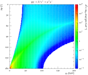
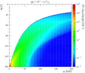
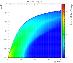
Figure 2: N²LO distributions in the transverse momentum of the leptonic system $q_{\mathrm{T}}$ and the opening angle between the two leptons in the transverse plane $\Delta\phi$.

Fig. 2 now details the distribution at N²LO, that is including terms up to $\mathcal{O}(\alpha_{s}^{2})$, in the transverse momentum of the leptonic system $q_{\mathrm{T}}$ and the opening angle between the two leptons in the transverse plane $\Delta\phi$. A regularising cut of $q_{\mathrm{T}}>1\,\text{GeV}$ is applied. As can be seen, the different sets of fiducial cuts necessitated by the differing measurable physics objects in each channel, induce differing coverages of the $q_{\mathrm{T}}$-$\Delta\phi$-plane. Although the fiducial regions overlap well at very small $q_{\mathrm{T}}$ and $\Delta\phi$, they illustrate that ratios between $Z$ and $W$ channels for the purpose of reweighting one channel to the other should not be taken single-differentially in $q_{\mathrm{T}}$ but need to take the constrained internal dynamics of the lepton system into account.

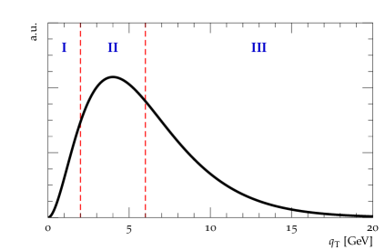
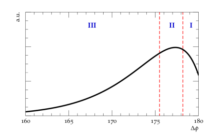
Figure 3: Illustration of the position of the three chosen slices in $q_{\mathrm{T}}$ and $\Delta\phi$  encompassing a region below (I), containing (II), and above (III) the Sudakov peak in each distribution.

Finally, Fig. 3 shows the qualitative behaviour of the single-differential behaviour of the matched cross section in $q_{\mathrm{T}}$ and $\Delta\phi$. In both distributions the typical resummed shape can be observed, exhibiting a Sudakov peak close to the singular point $(q_{\mathrm{T}},\Delta\phi)=(0,180^{\circ})$. It must be noted though, that the expression of the Sudakov peak in the $\Delta\phi$ spectrum strongly depends on the precise definition of the fiducial region. With these observations at hand, we define three different regions of interest for both spectra: (I) a region between the singular point and the Sudakov peak, (II) a region containing the Sudakov peak, and (III) a region beyond the Sudakov peak that includes the part of the spectrum where the resummation becomes unimportant. For the present study we therefore examine the $q_{\mathrm{T}}$ spectrum in three slices of $\Delta\phi$, $180^{\circ}>\Delta\phi>178.2^{\circ}$, $178.2^{\circ}>\Delta\phi>175.5^{\circ}$, and $175.5^{\circ}>\Delta\phi$, and the $\Delta\phi$ spectrum in three slices of $q_{\mathrm{T}}$, $1\,\text{GeV}<q_{\mathrm{T}}<2\,\text{GeV}$, $2\,\text{GeV}<q_{\mathrm{T}}<6\,\text{GeV}$, and $6\,\text{GeV}<q_{\mathrm{T}}$.

3.2 Validation

To begin with the examination of our result we first present a comparison of the resummed result, expanded to next-to-leading order (NLO${}_{\text{s}}$) and next-to-next-to-leading order (N²LO${}_{\text{s}}$), i.e. truncating at $\mathcal{O}(\alpha_{s})$ and $\mathcal{O}(\alpha_{s}^{2})$, respectively, to the exact full QCD result at the same order, NLO and N²LO. It needs to be noted that, contrary to the complete resummed result, the (expanded) fixed-order results diverge as $q_{\mathrm{T}}\to 0$. We thus, impose a cut of $q_{\mathrm{T}}>1\,\text{GeV}$ for the validation in this section, both for the $q_{\mathrm{T}}$ and $\Delta\phi$ spectra discussed in the following. The N³LO_s expansion of the resummed result will be compared with the corresponding full QCD computation in a future study.

Fig. 4 shows this comparison for the $q_{\mathrm{T}}$ spectra in the three slices in $\Delta\phi$ introduced earlier. In all three slices the agreement between the exact QCD result and the expanded resummed result derived from the soft-collinear effective theory is excellent for all three processes, $Z$, $W^{+}$, and $W^{-}$ production, under investigation. It is interesting to note that within a few percent the approximation in the soft-collinear effective theory holds to sizeable distances from the singular point at $(q_{\mathrm{T}},\Delta\phi)=(0\,\text{GeV},180^{\circ})$. In particular, deviations do not exceed 2% for $q_{\mathrm{T}}$ up to 10 GeV for all $\Delta\phi$ ranges, neither at NLO nor N²LO. These observations hold independent of the factorisation and renormalisation scale, as is indicated by the coincidence of the shown scale variation bands.

The situation is slightly different for the $\Delta\phi$ distributions in the three $q_{\mathrm{T}}$ slices depicted in Fig. 5. Here, the fixed-order expansion of the resummation very well coincides with the exact QCD calculation only in the first two slices for $q_{\mathrm{T}}$ smaller than 6 GeV. In the last $q_{\mathrm{T}}$ slice, well away from the singular point, the agreement is worse, ranging from around $5\%$ to 10%, with the best agreement unsurprisingly found on the Sudakov peak. Small effects due to limited statistics can be observed near the phase space boundaries, but do not impact our findings.

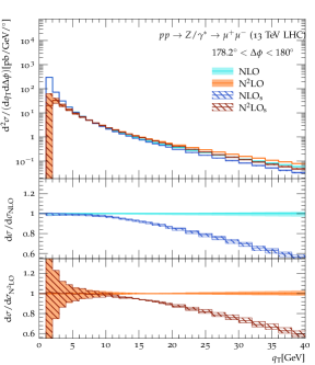
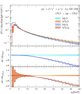
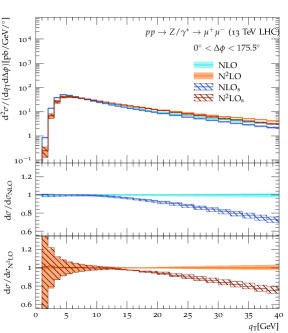
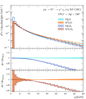
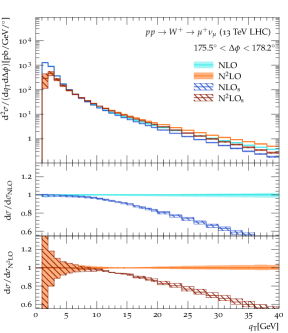
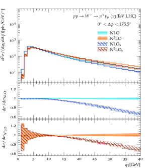
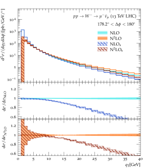
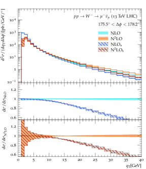
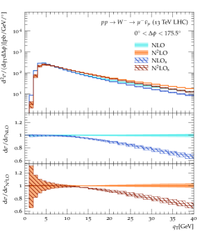
Figure 4: Comparison of the fixed-order $q_{\mathrm{T}}$ spectra in all three processes. N⁽²⁾LO denotes the fixed-order full QCD perturbative result, while N⁽²⁾LO${}_{\text{s}}$ is the fixed-order expansion of the SCET-based resummation.

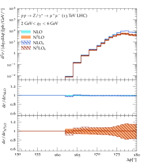
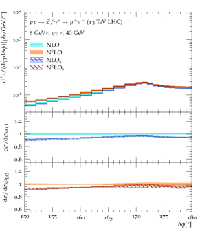
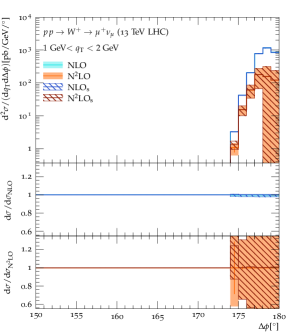
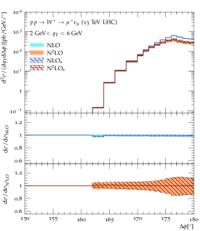
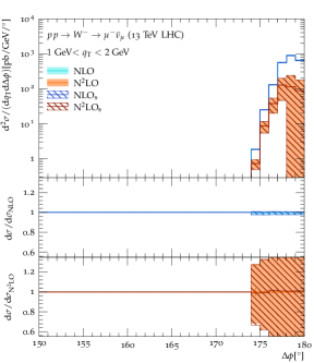
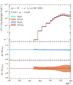
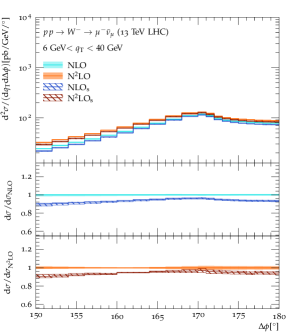
Figure 5: Comparison of the fixed-order $\Delta\phi$ spectra in all three processes. N⁽²⁾LO denotes the fixed-order full QCD perturbative result, while N⁽²⁾LO${}_{\text{s}}$ is the fixed-order expansion of the SCET-based resummation.

3.3 Resummation improved results

We now turn to examine our full resummation improved results, calculated according to eq. (2.37). Contrary to the fixed-order evaluation of the previous section, the behaviour of the cross section as we approach the singular point at $(q_{\mathrm{T}},\Delta\phi)=(0,180^{\circ})$ is regular and we can evaluate the complete $(q_{\mathrm{T}},\Delta\phi)$ plane. To arrive at our resummation improved results of this section, however, the governing eq. (2.35) still contains two terms that are separately diverging as the singular point is approached, originating in the behaviour of the full QCD fixed-order calculation and the fixed-order expansion of the resummation in the soft-collinear effective theory. To regulate their behaviour, following the results of Sec. 3.2, we set them to be exactly equal for $q_{\mathrm{T}}<1\,\text{GeV}$, leaving only the resummed result similar to the treatment in Refs. [180, 111]. Having said that, the most important question to answer, is the choice of matching scale $\mu_{Q}$. For this, we follow two arguments to guide us to our choice of matching scale.

Firstly, we want to restrict the resummation to the asymptotic regime where its intrinsic approximations are valid. Recalling that the resummation in eq. (2.29) is derived from the factorisation of eq. (2.4) where only the leading contributions in an expansion in $q_{\mathrm{T}}/M_{L}$ are kept, eq. (2.29) is valid only in the small $q_{\mathrm{T}}$ regime and thus should be disabled beyond it. To this end, the transition function $f(x)$ of eq. (2.36) is employed to provide a smooth transition from the resummed spectra to the fixed-order contribution in the matched result of eq. (2.35) within the interval $\mu_{Q}\mp\Delta q_{\mathrm{T}}$ with $\Delta q_{\mathrm{T}}\approx 4.6\,\text{GeV}$ with our choice of scales. We note that the value of $\mu_{Q}$ is related to the effective range of the $q_{\mathrm{T}}/M_{L}$ expansion. Following the spirit of [180] we determine that range by comparing in Fig. 4 the N²LO result with the corresponding expansion of the resummation N²LO_s. To be precise, we require the fixed-order expansion of the SCET approximation to deviate from the exact result by no more than 20%. For all three processes and $\Delta\phi$ slices we extract similar values, leading to a common choice of matching scale of $\mu_{Q}=16\,\text{GeV}$.

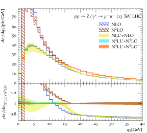
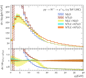
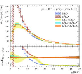
Figure 6: Single-differential cross section in $q_{\mathrm{T}}$ for all three processes. We compare the full QCD NLO and N²LO distributions to the resummation improved results, NLL^′+NLO, N²LL^′+N²LO, and N³LL^′+N²LO.

Secondly, we want the additional corrections introduced by the resummation with respect to the fixed-order calculation to be small or negligible at the matching scale. To evaluate this requirement, Fig. 6 is of particular interest. Here we observe that at values around the chosen matching scale $\mu_{Q}=16\,\text{GeV}$ the resummation improved results coincide with the pure fixed-order one to better than 3%. At this point, the reader is reminded that, although we are not comparing the pure resummation with the full QCD result but instead a result where the resummation at the scale $\mu_{Q}$ is already subjected to the suppression function $f(q_{\mathrm{T}})$ of eq. (2.36), the suppression function has the value $f(\mu_{Q})=0.5$. Therefore, we still find that the resummation and the fixed-order result still agree to better than 5% and resummation effects are no longer important. It is interesting to note that this observation holds for both N²LL^′+N²LO and N³LL^′+N²LO. The situation is slightly different for NLL^′+NLO. However, since this result is mainly included to illustrate the progression of the increased accuracy of our calculation we choose the same value for $\mu_{Q}$.

Analytically this can be understood in the following. In the above argument we are essentially evaluating the relative size of the contribution the resummation is supplying beyond the accuracy of the fixed-order calculation. These terms are of $\mathcal{O}(\alpha_{s}^{2}L^{4}+\alpha_{s}^{2}L^{3}+\ldots)$ for the NLL^′+NLO matched result, while they are of $\mathcal{O}(\alpha_{s}^{3}L^{6}+\alpha_{s}L^{5}+\ldots)$ for the N²LL^′+N²LO and N³LL^′+N²LO calculations, $L=\log(q_{\mathrm{T}}/M_{L})$. Now while $q_{\mathrm{T}}$ is small, these contributions are of the same order. Choosing a $\mu_{Q}$ sufficiently removed from the singular point, such that the ratio $q_{\mathrm{T}}/M_{L}$ is of $\mathcal{O}(1)$, $L$ follows a different power counting. Thus, the additional terms induced by the resummation with respect to the fixed-order calculation are indeed of higher-order in N²LL^′+N²LO and N³LL^′+N²LO than in NLL^′+NLO.

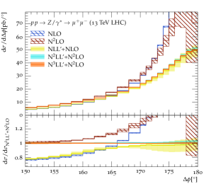
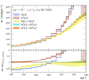
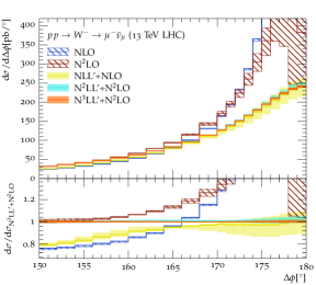
Figure 7: Single-differential cross section in $\Delta\phi$ for all three processes. We compare the full QCD NLO and N²LO distributions to the resummation improved results, NLL^′+NLO, N²LL^′+N²LO, and N³LL^′+N²LO.

With this choice of resummation scale the single-differential distributions in the leptonic transverse opening angle $\Delta\phi$ similarly receive substantial resummation effects, as shown in Fig. (7). Since the suppression function $f$ acts in another variable, no clear transition from one regime to the other can be observed at any order. We observe, however, that while at our highest order, N³LL^′+N²LO, all three processes behave extremely similarly and receive very similar resummation induced corrections to the N²LO result, this is markedly different at NLL^′+NLO accuracy. Here, the $W$ production channels receive somewhat larger corrections in the region between $\Delta\phi=150^{\circ}$ and $\Delta\phi=165^{\circ}$ than in $Z$ production.

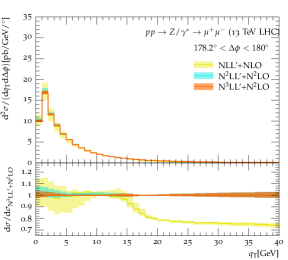
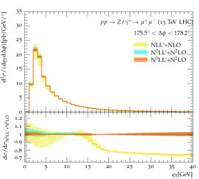
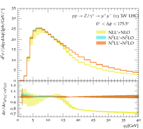
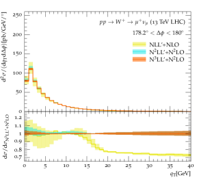
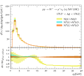
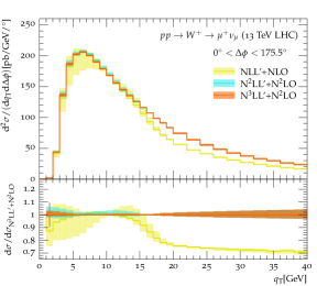
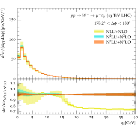
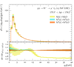
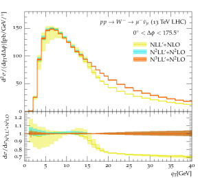
Figure 8: Double-differential cross section in $q_{\mathrm{T}}$ and three slices of $\Delta\phi$ for all three processes. We present the resummation improved results at NLL^′+NLO, N²LL^′+N²LO, and N³LL^′+N²LO accuracy.

With this global picture examined, we now turn to the aim of our study, the double-differential distributions. We again begin with the $q_{\mathrm{T}}$ spectra in our three chosen slices of $\Delta\phi$ in Fig. 8. While only the first slice for $\Delta\phi>175.5^{\circ}$ contains the singular point, all slices are close enough to the singularity that a Sudakov peak is formed. The description of this resummation region depends strongly on the order of logarithmic corrections included. While the central values do not change significantly order-by-order, validating our choice for the central scales involved in the resummation, the estimated uncertainty steadily decreases when going to higher orders. To be definite, the uncertainty in our lowest accuracy calculation (NLL^′) ranges from $-20\%$ to $+15\%$ around the central value around the Sudakov peak, independent of the $\Delta\phi$ slice, and involves a sizeable shape uncertainty as well. This shape uncertainty in particular differs in the region below the Sudakov peaks depending on $\Delta\phi$. Both uncertainties are reduced greatly when higher-order logarithmic corrections are included. At N²LL^′ they amount to $-4\%$ to $+7\%$ while at N³LL^′ they are reduced to $-2\%$ to $+4\%$.

Moving towards larger $q_{\mathrm{T}}$, the matching uncertainty tends to become comparable to the perturbative uncertainties in the resummation, dominating in particular NLL^′+NLO calculation around $\mu_{Q}$. As discussed above, the matching scale was chosen based on arguments for the highest precision calculation in this study and significant contributions of the resummation beyond the NLO fixed-order accuracy were found. Hence, this finding is not surprising. On the contrary, the matching uncertainty is substantially reduced in both the N²LL^′+N²LO and N³LL^′+N²LO calculations, not exceeding $\pm 1\%$ in the latter. At even higher transverse momenta the fixed-order calculation dominates the spectrum and its usual behaviour and uncertainties are recovered.

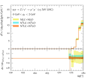
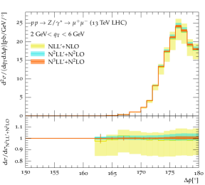
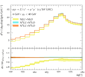
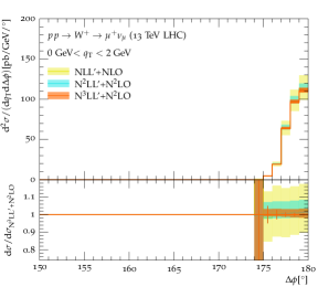
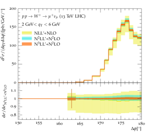
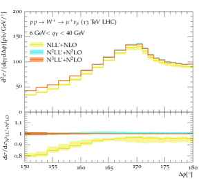
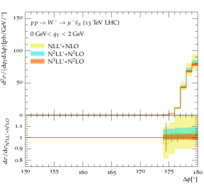
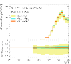
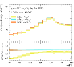
Figure 9: Double-differential cross section in $\Delta\phi$ and three slices of $q_{\mathrm{T}}$ for all three processes. We present the resummation improved results at NLL^′+NLO, N²LL^′+N²LO, and N³LL^′+N²LO accuracy.

Finally, we examine the resummation improved results for the $\Delta\phi$ spectra in the three chosen $q_{\mathrm{T}}$ regions. Recall that the first region with transverse momenta smaller than 2 GeV resides entirely below the Sudakov peak in the transverse momentum spectrum, while the second one contains the peak, and the third region with $q_{\mathrm{T}}>6\,\text{GeV}$ resides entirely beyond the Sudakov peak. Consequently, very different behaviour can be observed despite the per-bin-cross sections being of similar orders of magnitude. The results of our computation for the $\Delta\phi$ spectra are shown in Fig. 9. As all three processes exhibit a very similar behaviour we continue to discuss them simultaneously.

In the lowest $q_{\mathrm{T}}$ region, which probes the region below the Sudakov peak in the $q_{\mathrm{T}}$ spectrum, near back-to-back topologies are favoured unsurprisingly and resummation effects dominate the calculation throughout. Consequently, as observed before, the central values of our three predictions of increasing logarithmic accuracies agree very well. Their uncertainties have nearly no $\Delta\phi$ dependence and are steadily decreasing with the increasing accuracy of the resummation, reaching $-1\%$ to $+2\%$ in the N³LL^′ case.

In the intermediate $q_{\mathrm{T}}$ slice, focussing on the region around the Sudakov peak in the $q_{\mathrm{T}}$ spectrum, a peaked structure is developing. Still, the distribution is dominated by resummation effects, leading again very well agreeing central values, their uncertainties being dictated by the order of the logarithms included in the exponent. We, thus, find a variation of $\pm 1\%$ in our most accurate calculation. This time, however, there is a slight shape to these scale uncertainties, predominantly in the back-to-back region.

The third $q_{\mathrm{T}}$ slice, located entirely above the $q_{\mathrm{T}}$ Sudakov peak, now sees a stronger impact of the full QCD fixed-order calculations. Hence we find the central values no longer agree, partially reflecting the difference in cross section between the NLO and N²LO predictions for the spectrum. The increasing importance of the full QCD fixed-order part for smaller $\Delta\phi$ likewise explains the shape corrections at higher order. Still, the uncertainties are much reduced in our highest precision calculation at N³LL^′+N²LO accuracy, being smaller than $\pm 1\%$ throughout.

Finally, please note that the smallest $\Delta\phi$ bin in the lower two $q_{\mathrm{T}}$ slices carries almost no cross section and, thus, suffers from larger statistical uncertainties.

3.4 The $W^{\pm}/Z$ and $W^{+}/W^{-}$ correlations

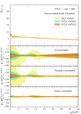
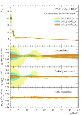
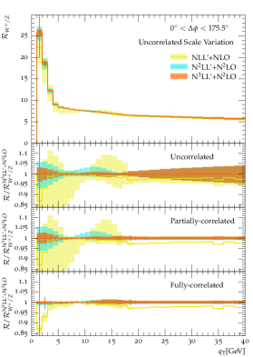
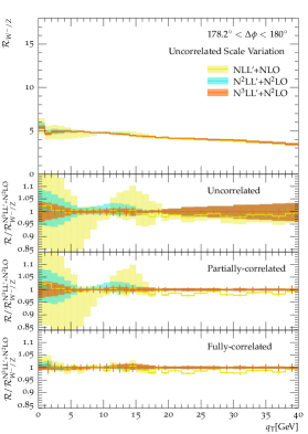
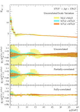
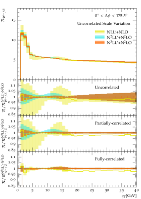
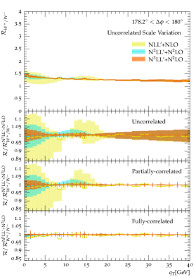
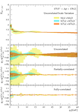
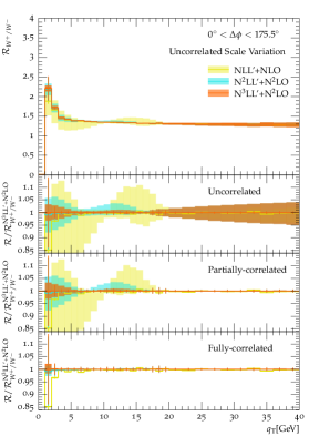
Figure 10: Double-differential cross section ratios in $q_{\mathrm{T}}$ and three slices of $\Delta\phi$ for all three processes. We present the resummation improved results at NLL^′+NLO, N²LL^′+N²LO, and N³LL^′+N²LO accuracy.

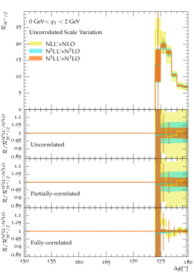
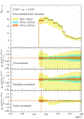
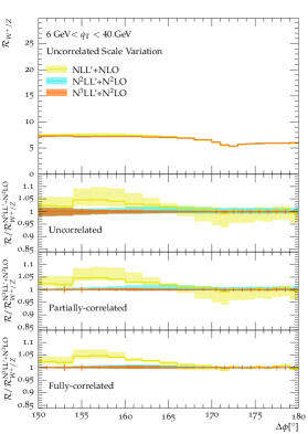
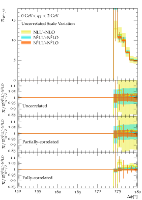
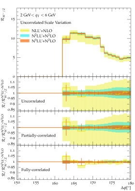
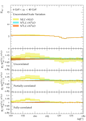
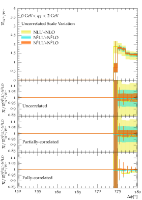
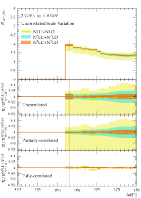
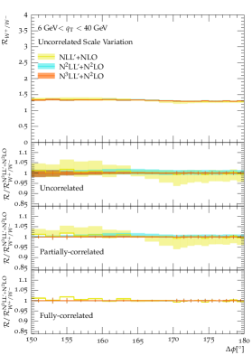
Figure 11: Double-differential cross section ratios in $\Delta\phi$ and three slices of $q_{\mathrm{T}}$ for all three processes. We present the resummation improved results at NLL^′+NLO, N²LL^′+N²LO, and N³LL^′+N²LO accuracy.

With the double-differential resummation-improved cross sections of the previous section at hand we finally turn towards cross section ratios. They are useful to obtain high-precision $W^{+}$ and $W^{-}$ production data, by measuring the fully and precisely reconstructible cross sections in $Z$ production and applying the following theory predictions, see e.g. Refs. [12]. Similarly, the $W^{+}$ to $W^{-}$ ratio is of interest for PDF extractions, see e.g. [13]. A key question, however, is how to determine the uncertainties of such a ratio. The main bottleneck is the fundamental lack of statistical interpretation of the theoretical uncertainties on (multi-)differential cross sections as presented so far. Thus, in particular various assumptions about their (non-)correlation in the numerator and denominator of the $R_{W^{\pm}/Z}$ have to be made. In the following, we present results for the following three correlation assumptions:

• Uncorrelated. The scales of the $W^{\pm}$ and $Z$ processes are assumed to be completely uncorrelated. All scales in the numerator and denominator are varied independently. This corresponds to the assumption that both processes have no common structure in the form of their higher-order corrections or input functions, such as the PDFs. As this is known not to be the case, the uncertainties on the ratio obtained this way are likely to be severely overestimated.

• Fully correlated. All scales of the $W^{\pm}$ and $Z$ processes are assumed to be completely correlated. They are thus varied by a common factor in the numerator and denominator simultaneously. This corresponds to the assumption that both processes have exactly the same structure in the form of their higher-order corrections and input functions, such as the PDFs. As this is known not to be the case, the uncertainties on the ratio obtained this way are likely to be severely underestimated.

• Partially correlated. A careful analysis of the internal structure of the higher-order corrections to $W^{\pm}$ and $Z$ production allows to carefully assess which corrections have identical (or at least very similar) structures and which differ. This allows, to first approximation, to select a subset of scales to fully correlate, uncorrelating the rest. Following a detailed analysis of the derivations of Sec. 2, we find that the singlet contributions to $Z$ production are numerically small, see App. A. In consequence, both the hard and soft functions for $W^{\pm}$ and $Z$ decays show the same dependence on the respective scales. Differences, however, occur for the beam functions, arising in the different composition of initial states in all three processes. We thus choose to fully correlate the variation of all scales except for $\mu_{b}$ and $\nu_{b}$, which we fully uncorrelate.

Figs. 10 and 11 now show the ratios $\mathcal{R}_{W^{+}/Z}$, $\mathcal{R}_{W^{-}/Z}$, and $\mathcal{R}_{W^{+}/W^{-}}$ for all three definitions of their uncertainties detailed above. In the following, we will discuss the different features of both their central values and uncertainties separately.

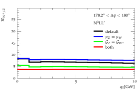
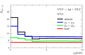
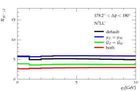
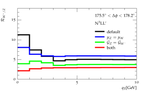
Figure 12: Double-differential cross section ratios $\mathcal{R}_{W^{+}/Z}$ and $\mathcal{R}_{W^{-}/Z}$ in $q_{\mathrm{T}}$ and the two $\Delta\phi$ slices closest to the singular region. We present the resummed results at N³LL^′ accuracy for the default parameters and fiducial regions used in all physical predictions (black), for the default parameters and the $Z$ production phase space $\mathcal{G}_{Z}$ adapted to the $W^{\pm}$ production phase space $\mathcal{G}_{W^{\pm}}$ (green), for the $Z$ boson mass set equal to the $W$ boson mass and default fiducial regions (blue), and for both adaptations of the $Z$ production parameters (red), see text for details.

Central values.

The central values of the cross section ratios are of course unaffected by the precise definition of the uncertainty band. Instead, they are largely determined by the slightly different location of the Sudakov peak induced by the mass difference, the different $x$-dependence of the contributing parton distributions, and the slightly different fiducial phase spaces. In addition, they only exhibit a small dependence on the perturbative order at which they are calculated. In fact, with respect to the perturbative stability of these ratios, we observe only minor corrections on the level of up to 2% in $\mathcal{R}_{W^{+}/Z}$ and $\mathcal{R}_{W^{-}/Z}$, and much smaller in $\mathcal{R}_{W^{+}/W^{-}}$, when increasing the intrinsic accuracy of the resummation-improved calculation from NLL^′+NLO to N³LL^′+N²LO.

Further, the cross section ratios depend only weakly on the transverse momentum of the reconstructed vector boson for $q_{\mathrm{T}}>5\,\text{GeV}$. Below that value, in the vicinity and left flank of the Sudakov peak, all three ratios exhibit a marked increase. As alluded to earlier, this increase is induced by the differing precise locations of the Sudakov peak in each process. Fig. 12 investigates this phenomenon more closely, by

• setting complex mass of the $Z$ boson to that of the $W$ boson in the propagator only, keeping all other parameters at the default values,

• replacing the fiducial phase space definition for the $Z$ production channel, $\mathcal{G}_{Z}$, by that of the $W^{\pm}$ channel, $\mathcal{G}_{W^{\pm}}$ with the $\ell^{\mp}$ taking the role of the neutrino, and

• applying both modifications a) and b).

This leaves the differences due to the participating parton fluxes and the different spin-structures in the underlying EW couplings. We find that in the $q_{\mathrm{T}}$ spectra the majority of the effect is induced by the differing fiducial regions, with smaller additional corrections stemming from the different $W$ and $Z$ boson masses. With both effects accounted for, the ratios are nearly $q_{\mathrm{T}}$ and $\Delta\phi$ independent, with the remaining small deviations attributed to the PDFs and the different spin-structures of the underlying EW coupling.

It needs to be noted, though, that the difference in fiducial phase spaces between $W^{\pm}$ and $Z$ measurements in the $W$-boson mass measurement [12] was larger than the one used here. Hence, the effect can be estimated to have been larger in that phase space as well.

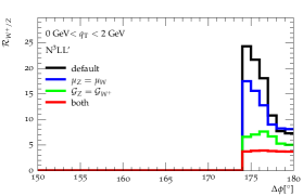
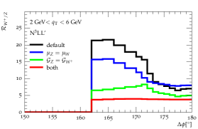
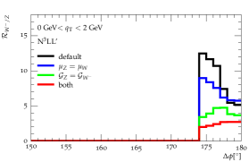
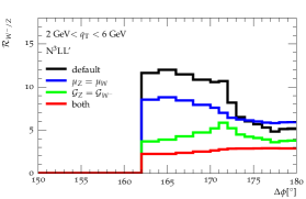
Figure 13: Double-differential cross section ratios $\mathcal{R}_{W^{+}/Z}$ and $\mathcal{R}_{W^{-}/Z}$ in $\Delta\phi$ and the two $q_{\mathrm{T}}$ slices closest to the singular region. We present the resummed results at N³LL^′ accuracy for the default parameters and fiducial regions used in all physical predictions (black), for the default parameters and the $Z$ production phase space $\mathcal{G}_{Z}$ adapted to the $W^{\pm}$ production phase space $\mathcal{G}_{W^{\pm}}$ (green), for the $Z$ boson mass set equal to the $W$ boson mass and default fiducial regions (blue), and for both adaptations of the $Z$ production parameters (red), see text for details.

The $\Delta\phi$ spectra show a stronger variation of the central value of the cross section ratio, increasing to up to a factor of three above their value far away from the Sudakov peak in both $q_{\mathrm{T}}$ and $\Delta\phi$, in particular in the first two regions. This increase, however, appears on the far side of the peak away from the back-to-back region, in contrast to the increase observed in the $q_{\mathrm{T}}$ spectra. Nonetheless, its origin can be traced to the same factors as for the $q_{\mathrm{T}}$ spectra in Fig. 13, the different definitions of the fiducial phase space in $W$ and $Z$ production and the different $W$ and $Z$ boson masses. To be specific, we observe that when both effects are accounted for the ratio is nearly independent of both $q_{\mathrm{T}}$ and $\Delta\phi$. This also means that the remaining PDF dependence is small.

At this point it is important to note that although both the fiducial phase spaces in $W^{+}$ and $W^{-}$ appear to be the same, they are not. The reason is that, in terms of spin-correlation the anti-neutrino produced in the decay of the $W^{-}$ takes the role of the charged lepton in the decay of the $W^{+}$, but not in the observable definition. This is compounded by the fact that, out of the three processes under consideration here, $W^{+}$ and $W^{-}$ show the largest divergence of the contributing partonic fluxes, imparting differing rapidity distributions on the produced boson and, thus, slightly different effects of the fiducial cuts. These factors add up to explain the remaining small, but non-negligible $q_{\mathrm{T}}$ and $\Delta\phi$ dependence of $\mathcal{R}_{W^{+}/W^{-}}$.

Finally, the ratios $\mathcal{R}_{W^{+}/Z}$, $\mathcal{R}_{W^{-}/Z}$, and $\mathcal{R}_{W^{+}/W^{-}}$ are nearly flat in the third region containing events with $q_{\mathrm{T}}>6\,\text{GeV}$, its only structure being induced mostly by the difference in the fiducial phase space in $W$ and $Z$ boson production.

Uncertainties.

The uncertainty of the cross section ratios follows the pattern laid out in their definition: while the fully-correlated case leads to vanishingly small uncertainties, smaller than 1% in most regions (in fact, the largest surviving uncertainty is related to the matching procedure), the fully-uncorrelated case lies on the opposite end of the spectrum with uncertainties of $\pm 4\%$ for our best calculation at N³LL^′+N²LO accuracy both in the fixed-order region and the resummation region. The partially-correlated ansatz so far yields the, in our judgement, most reliable result, ranging from $\pm 1\%$ in the fixed-order region where the respective scales are correlated and $\pm 3\%$ in the resummation region. In particular, it is interesting to note that the beam function uncertainties are the driving force of the resummation uncertainties overall, reinforcing the difference in contributing parton fluxes as a driving factor for the details of the ratio overall. Similarly, we observe that, apart from the fully-correlated uncertainty estimate, the uncertainty for $\mathcal{R}_{W^{+}/W^{-}}$ largely follows the pattern of $\mathcal{R}_{W^{+}/Z}$ and $\mathcal{R}_{W^{-}/Z}$  both qualitatively and quantitatively.

4 Conclusions

In this paper we have computed the single-differential $q_{\mathrm{T}}$ and $\Delta\phi$ as well as the double-differential $(q_{\mathrm{T}},\Delta\phi)$ spectra for inclusive $Z$, $W^{+}$, and $W^{-}$ production in the experimentally accessible fiducial phase space up to N³LL^′+N²LO accuracy resumming small transverse momentum logarithms. Besides the essential inclusion of the third-order soft and beam functions, the resummation features the incorporation of leptonic power corrections and the singlet contribution into the hard sector. The leptonic power corrections have been found to extend the region of validity of the approximate SCET result. The singlet contributions, on the other hand, characterised by topologies where the external quarks do not directly couple to the electroweak gauge boson, enter the $Z$ boson production process at second and third order in $\alpha_{s}$, and have been found to yield corrections of similar size as the non-singlet third order ones, and are thus non-negligible at N³LL^′.

In our numerical evaluation we first confronted the approximate results derived from the SCET with the exact ones and excellent agreement has been observed in the asymptotic regime. We then computed the resummation-improved single- and multidifferential distributions at NLL^′+NLO, N²LL^′+N²LO and N³LL^′+N²LO and found excellent perturbative convergence in the asymptotic regime, i.e. the higher order predictions and their estimated uncertainties are fully contained in the lower order uncertainty band. Further, the respective uncertainties themselves are systematically reduced to the level around 4% or less at N³LL^′+N²LO.

In addition, we computed the ratios $\mathcal{R}_{W^{+}/Z}$, $\mathcal{R}_{W^{-}/Z}$, and $\mathcal{R}_{W^{+}/W^{-}}$ of these calculations and estimated their uncertainty assuming no correlation, full correlation, and, as our best prediction, a partial correlation of the scale variations in the numerator and denominator making up the uncertainty. For the partial correlation case in particular, a careful assessment of the internal structure of our calculation allowed to identify identical (or very similar) components and structures that differed between the three different processes. Consequently, the scales used to estimate the uncertainties originating in similar components were correlated while scales used to estimate the uncertainties originating in differing structures were varied independently. The main driver for the differences were identified to be related to the incident beams and the partonic fluxes initiating the respective processes.

In summary, we determine the ratios with relative uncertainties of less than 1%, rising to 3-4% in the resummation region at N³LL^′+N²LO accuracy. The shape of the ratios, although largely perturbatively stable, is not constant but shows a strong impact of the fact that the Sudakov peak is located at slightly different positions in all three processes. This observation is the consequence of three main factors:

• the difference in the $W$ and $Z$ boson masses,

• the different partonic fluxes contributing to the three processes and the different $(x,Q)$-dependence of the $u$ and $d$ valence quarks in particular, and

• the difference in the fiducial regions for $\ell^{+}\ell^{-}$ and $\ell^{\pm}+\displaystyle{\not}p_{\mathrm{T}}$ final states.

The latter is, in fact, the dominating factor in the $\Delta\phi$ and low-$q_{\mathrm{T}}$-dependence of the $\mathcal{R}_{W^{+}/Z}$ and $\mathcal{R}_{W^{-}/Z}$ ratios.

With the presented calculation at hand, precise predictions for both absolute fiducial multidifferential cross sections and their ratios that are vital for the LHC’s precision measurements programme can be made. Nonetheless, important contributions from higher-order corrections originating in the electroweak sector of the Standard Model are not included in our calculation yet, and we leave their investigation to a future publication. Similarly, we have for now not included non-perturbative corrections that are expected to give non-negligible contributions in particular at small transverse momenta or large azimuthal separations. Their reliable modelling is intricate, including both flavour and $x$-dependent contributions, and goes beyond the scope of this paper. It will also be addressed in a future publication.

Acknowledgements

WJ is grateful to Xuan Chen and Markus Ebert for helpful discussions on the matching procedure. WJ also thanks Konstantin G. Chetyrkin and Thomas Gehrmann for constructive discussions on the singlet hard functions. MS is funded by the Royal Society through a University Research Fellowship (URF\R1\180549). WJ and MS are supported by a Royal Society Enhancement Award (RGF\EA\181033 and CEC19\100349). This work has received funding from the European Union’s Horizon 2020 research and innovation programme as part of the Marie Sklodowska-Curie Innovative Training Network MCnetITN3 (grant agreement no. 722104).

Appendix A Impact of the singlet contributions

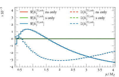
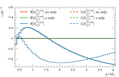
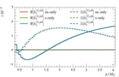
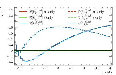
Figure 14: Numeric results for the hard coefficients $h_{\gamma}^{(3)}$ (left) and $h_{Z,V}^{(3)}$ (right) in the vector current.

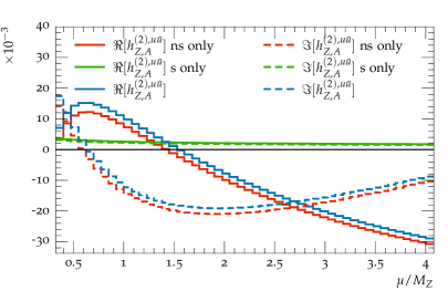
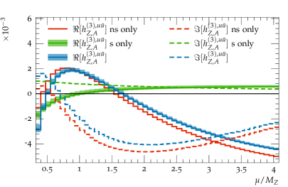
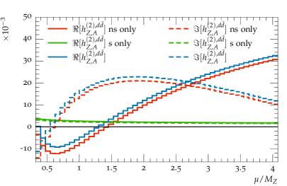
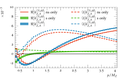
Figure 15: Numeric results for the hard coefficients $h_{Z,A}^{(2)}$ (left) and $h_{Z,A}^{(3)}$ (right) in the axial-vector current.

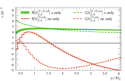
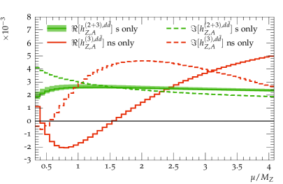
Figure 16: Comparison of the total singlet contribution to the third-order non-singlet contribution.

In this appendix we present a quantitative discussion of the singlet contributions to the hard function. To this end, we re-express the hadronic current $H^{\mu,ij}$ of (2.17) in the following form,

$$\begin{split}H^{\mu,ij}_{\gamma}=&\;\left(g_{\gamma}^{q_{i}}C_{\mathrm{ns}}+g_{\gamma}^{\scriptscriptstyle\Sigma}C_{\mathrm{s}}^{V}\right)\mathcal{V}^{\mu}_{ij}\equiv\,e\,\mathcal{V}^{\mu}_{ij}\,\sum_{m}\,h_{\gamma}^{(m),ij}\,,\\ H^{\mu,ij}_{Z,V}=&\;\left(g_{V}^{q_{i}}C_{\mathrm{ns}}+g_{V}^{\scriptscriptstyle\Sigma}C_{\mathrm{s}}^{V}\right)\mathcal{V}^{\mu}_{ij}\equiv\,\frac{e}{s_{w}\,c_{w}}\,\mathcal{V}^{\mu}_{ij}\sum_{m}\,h_{Z,V}^{(m),ij}\,,\\ H^{\mu,ij}_{Z,A}=&\;g_{A}\left[\left(2T_{q_{i}}+\frac{1}{N_{F}}\right)C_{\mathrm{ns}}+C_{t}C_{\mathrm{s}}^{A}\right]\mathcal{A}^{\mu}_{ij}\equiv\,g_{A}\,\mathcal{A}^{\mu}_{ij}\sum_{m}\,h_{Z,A}^{(m),ij}\,,\end{split}$$ (A.1)

where the coefficients $h_{\gamma}^{(m),ij}$, $h_{Z,V}^{(m),ij}$ and $h_{Z,A}^{(m),ij}$ represent the $\mathcal{O}(\alpha_{s}^{m})$ corrections to the hadronic currents. During our calculations here, the invariant mass $M_{L}$ is specifically fixed to $m_{Z}$, while the scale $\mu$ is left as a variable.

Fig. 14 exhibits the size of the non-singlet N³LO coefficients $h_{\gamma}^{(3)}$ and $h_{Z,V}^{(3)}$ for the $u\bar{u}$ and $d\bar{d}$ partonic channels. As the singlet contribution to the vector current is forbidden at two loop level by $C$-parity, we plot only the third order therein. The numerical results computed in three different ways are displayed: 1) the $\mathcal{O}(\alpha_{s}^{3})$ correction with both the non-singlet coefficient $C_{\mathrm{ns}}$ and the singlet coefficient $C_{\mathrm{s}}^{V}$ included; 2) the same $\mathcal{O}(\alpha_{s}^{3})$ correction including only the non-singlet contribution $C_{\mathrm{ns}}$; and 3) the $\mathcal{O}(\alpha_{s}^{3})$ singlet contribution $C_{\mathrm{s}}^{V}$. It is seen that for the entire $\mu$ range, the both the real and the imaginary part of the full $\mathcal{O}(\alpha_{s}^{3})$ correction (in blue lines) almost coincide with the pure non-singlet ones (in red lines), and the singlet contributions (in green lines) are negligible. This indicates that at least up to $\mathcal{O}(\alpha_{s}^{3})$, the role played by the singlet terms in the vector hadronic current is of little phenomenological impact. Moreover, it can also be observed that the full and non-singlet results of $u\bar{u}$ initial state are curved in the opposite direction to the $d\bar{d}$ ones. This is caused by the different charges and weak isospins of the $u$ and $d$ quarks. As shown in eq. (2.17), given the negligible singlet vector terms, the vector current hard coefficients between different initial states can be related as follows

$$\begin{split}\frac{h_{\gamma}^{(3),u\bar{u}}}{h_{\gamma}^{(3),d\bar{d}}}&\sim\frac{Q_{u}}{Q_{d}}=-2\,,\\ \frac{h_{Z,V}^{(3),u\bar{u}}}{h_{Z,V}^{(3),d\bar{d}}}&\sim\frac{T_{u}^{3}-2Q_{u}s_{w}^{2}}{T_{d}^{3}-2Q_{d}s_{w}^{2}}\sim-\frac{1}{2}\,.\\ \end{split}$$ (A.2)

Here the flipping signs account for the different curvatures as observed, and the proportions derived in the last step give the relationship of the magnitudes of the $u\bar{u}$ and $d\bar{d}$ initiated results.

In Fig. 15, the magnitudes of the real and imaginary parts of axial-vector current hard coefficients are depicted. As the singlet contribution here starts at $\mathcal{O}(\alpha_{s}^{2})$, we show both $h_{Z,A}^{(2)}$ and $h_{Z,A}^{(3)}$. In complete analogy to the vector current coefficients, we here also graph the three types of outputs therein: 1) the full result calculated as eq. (2.17); 2) the non-singlet one including $C_{\mathrm{ns}}$ only; and 3) the singlet one which is the difference between the previous two cases. Contrary to Fig. 14, the axial-vector singlet terms give an unignorable contribution here for all values of $\mu$, but in particular for values of $\mu$ close to 0.5 or 1.5 where either the real or imaginary part of the non-singlet contribution vanishes. In the region $\mu\sim m_{Z}$, which is the default hard scale taken in the resummation in this paper (see eq. (3.4)), the singlet terms can account for around $20\%$ of the real contributions of the full results in $\mathcal{O}({\alpha_{s}^{2}})$, and nearly $40\%$ in $\mathcal{O}({\alpha_{s}^{3}})$. In the imaginary parts, it is also noted that more than $10\%$ of $\Im[h_{Z,A}^{(2),u\bar{u}}]$ and $\Im[h_{Z,A}^{(2),d\bar{d}}]$ is made up of the singlet terms for the majority of the $\mu$ range, and although at the third order accuracy the singlet terms experience zeros in the vicinity of $\mu=m_{Z}$, its proportions can recover to $\sim 10\%$ when $\mu/m_{Z}$ exceeds $2$. Furthermore, one interesting phenomenon in Fig. 15 is that the singlet contributions remain the same in the $u\bar{u}$ and $d\bar{d}$ initial states, but the non-singlet lines are curved in the different directions. The reason can be found in eq. (2.17). Therein the non-singlet contribution $C_{\mathrm{ns}}$ is directly proportional to the weak isospin of the initial parton, $T_{q_{i}}$, whilst the singlet terms $C_{t}C_{\mathrm{s}}^{A}+C_{\mathrm{ns}}/N_{F}$ are universal for all initial states. Therefore, after excluding the singlet terms, the $h_{Z,A}^{(2,3),u\bar{u}}$ results are actually taking the opposite numbers of those for the $d\bar{d}$ channel, while the singlet terms hold. Please note that we have added an uncertainty band to the results of $C_{\mathrm{s}}^{A,(3)}$ to account for the uncertainty arising from the finite terms, see eq. (C.9) and discussion thereafter. The error estimation is carried out by varying $c_{\text{s}}^{A,(3)}$ around the default choice as $[\tfrac{1}{2},2]\cdot C_{\text{ns}}^{(3)}|_{{}_{L_{H}=0}}$.

To further explore the properties of the axial-vector singlet terms, we confront the whole singlet contribution (the sum of the $\mathcal{O}(\alpha_{s}^{2})$ and $\mathcal{O}(\alpha_{s}^{3})$ corrections) with the non-singlet $h_{Z,A}^{(3)}$s in Fig. 16. It is seen that for the majority of the $\mu$ range, the singlet contribution takes the comparable magnitude to the third-order non-singlet result. Especially in the $\mu\sim m_{Z}$ region, the singlet terms approach $\Im[h_{Z,A}^{(3),d\bar{d}}]$ but are even greater than $\Re[h_{Z,A}^{(3),u\bar{u}}]$, $\Im[h_{Z,A}^{(3),u\bar{u}}]$ as well as $\Re[h_{Z,A}^{(3),d\bar{d}}]$ in magnitude. In fact, this observation can substantially highlight the importance of the singlet terms in the resummation. As shown in Table. 1, the resummation at N²LL^′ requires the $\mathcal{O}(\alpha_{s}^{2})$ hard function, whilst the N³LL^′ accuracy needs those up to the third order. So if only a precision of the order of $10\%$ of the $\mathcal{O}(\alpha_{s}^{2})$ correction is needed, the singlet terms could be neglected at the N²LL^′ accuracy in a numerically approximate sense. Nevertheless, as the complete singlet corrections are of the same magnitude as, if not larger than, the third-order non-singlet corrections, their inclusion is mandatory for a meaningful and robust N³LL^′ resummation.

Appendix B Impact of leptonic power corrections

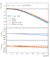
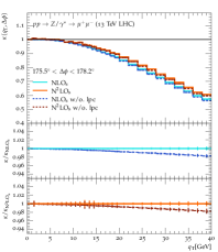
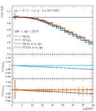
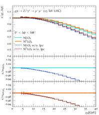
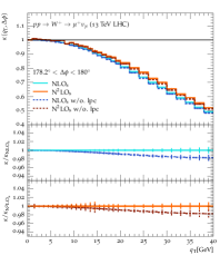
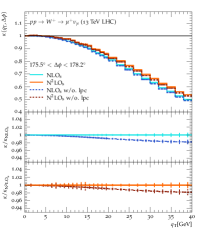
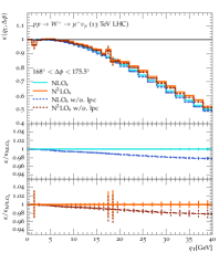
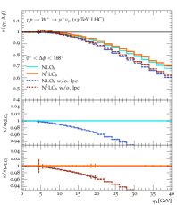
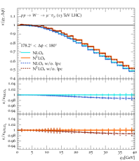
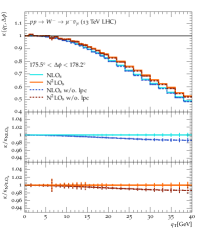
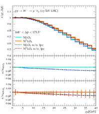
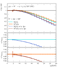
Figure 17: Numeric impacts of the leptonic power corrections on the $q_{\mathrm{T}}$ spectra.

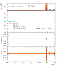
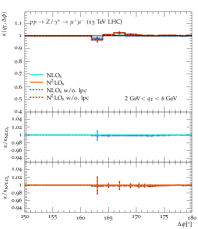
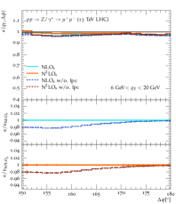
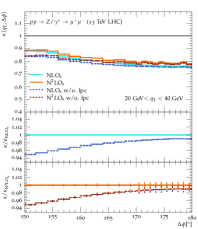
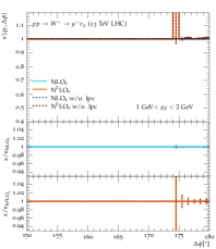
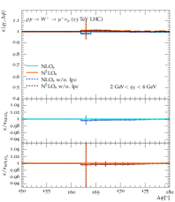
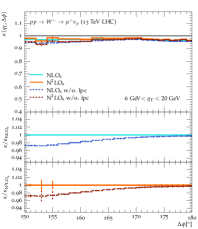
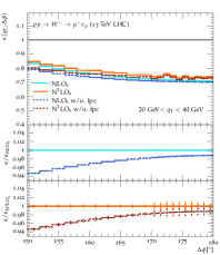
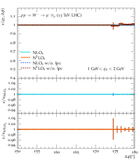
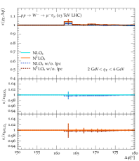
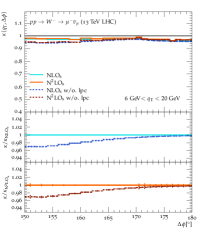
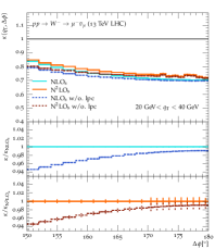
Figure 18: Numeric impacts of the leptonic power corrections on the $\Delta\phi$ spectra.

In eq. (2.34), the Lorenz-transformation matrix $\Lambda_{\ell}(\vec{q}_{\mathrm{T}})$ has been incorporated into the hard functions for including the leptonic power corrections. In this part, we will investigate its numerical influences on the double-differential observable ${\rm d}^{2}\sigma/({\rm d}q_{\mathrm{T}}{\rm d}\Delta\phi)$. To this end, we define the ratio of the approximate results to the exact ones as follows,

$$\kappa(q_{\mathrm{T}},\,\Delta\phi)\equiv\frac{{\rm d}^{2}\sigma_{\mathrm{exp}}/({\rm d}q_{\mathrm{T}}{\rm d}\Delta\phi)}{{\rm d}^{2}\sigma_{\mathrm{f.o.}}/({\rm d}q_{\mathrm{T}}{\rm d}\Delta\phi)},$$ (B.1)

where $\sigma_{\text{f.o.}}$ denotes the exact fixed-order perturbative result. $\sigma_{\mathrm{exp}}$ represents the perturbative expansions of the resummed distribution in eq. (2.29). For comparison, we will calculate $\sigma_{\mathrm{exp}}$ in two different ways: with or without $\Lambda_{\ell}(\vec{q}_{\mathrm{T}})$ contributions. While the result experienced eq. (2.34) is still named $\mathrm{N^{(m)}LO}_{\mathrm{s}}$, same as those in Figs. (4-5), those excluding $\Lambda_{\ell}(\vec{q}_{\mathrm{T}})$ effects are labelled as “$\mathrm{N^{(m)}LO}_{\mathrm{s}}$ w/o. lpc”. Here the superscript “m” specifies the expansion order in $\alpha_{s}$. Throughout this section, the results in former case will be depicted in the solid lines, and to distinguish, the dashed ones illustrate the later case.

In Fig. 17, we exhibit the numerical results for $\kappa(q_{\mathrm{T}},\,\Delta\phi)$ after integrating out $\Delta\phi$ over the following four intervals:

1) 178 .2∘	$<\Delta\phi<$	180∘;
2) 175 .5∘	$<\Delta\phi<$	178.2∘;
3) 168∘	$<\Delta\phi<$	175.5∘;
4) 0∘	$<\Delta\phi<$	168∘.

In the small $q_{\mathrm{T}}$ regime, the $\kappa$ distributions in the four slices all approach the unity and the differences due to the leptonic power corrections are insensible. This phenomenon is in agreement with the observations in Sec. 3.2 and also validates the leading power factorization in eq. (2.4). However, with the increase in the $q_{\mathrm{T}}$, the power corrections start to manifest themselves. For instance, in the intermediate region $q_{\mathrm{T}}\sim 20$ GeV, one can find that the $\kappa$ spectra obviously deviate from the unity grid and furthermore the discrepancies arising from the $\Lambda_{\ell}(\vec{q}_{\mathrm{T}})$ incorporation emerge. One interesting phenomenon is that differing from the first three slices, the $\kappa$ spectra in the last slice are fairly sensitive to the leptonic power corrections. To be specific, around the point $q_{\mathrm{T}}=25$ GeV, the $\Lambda_{\ell}(\vec{q}_{\mathrm{T}})$ incorporations in the first three slices improve the dashed lines by nearly $1\%$ towards the “f.o.” ones, whilst it escalates to $5\%$ for the last slice.

To interpret this, note the topological configuration of final leptons in the fourth slice considerably differs from the others. For the first three slices, as required by the small value of $(\pi-\Delta\phi)$, the final leptons are almost in the back to back configuration. So for the $q_{\mathrm{T}}\geq 25$ GeV region, the direction of $\vec{q}_{\mathrm{T}}$ tends to be aligned with $\hat{\vec{p}}_{{}_{\ell,\mathrm{T}}}$ in the transverse plane, so as to avoid the energetic recoil enhancing the $(\pi-\Delta\phi)$ value. Here $\hat{\vec{p}}_{{}_{\ell,\mathrm{T}}}$ represents the (anti-)lepton momentum in the rest frame of the lepton pair. Given the limit $\vec{q}_{\mathrm{T}}\parallel\hat{\vec{p}}_{{}_{\ell,\mathrm{T}}}$, the $\Lambda_{\ell}(\vec{q}_{\mathrm{T}})$ matrix acts only on the time-like and the longitudinal components of $L_{V}$, whereas the later case is only able to polarize perpendicularly to $\hat{\vec{p}}_{{}_{\ell,\mathrm{T}}}$ in the massless limit. After the contraction, the $\Lambda_{\ell}(\vec{q}_{\mathrm{T}})$ matrix is effectively reduced to the metric tensor and therefore gives rise to mild influences in the first three slices. The situation in the last slice is however different. A variety of $(\pi-\Delta\phi)$ therein can encourage the stronger recoils against lepton momenta, so that $\vec{q}_{\mathrm{T}}$ is capable of developing sizable perpendicular component with respect to $\hat{\vec{p}}_{{}_{\ell,\mathrm{T}}}$, which in turn permits $\Lambda_{\ell}(\vec{q}_{\mathrm{T}})$ non-trivially coupled with $L_{V}$.

With particular attention is that except for the boundary bins which suffer from statistical issues, the $\kappa$ values are all enhanced towards the unity grid after incorporating the leptonic power correction matrix $\Lambda_{\ell}(\vec{q}_{\mathrm{T}})$. This indicates that $\Lambda_{\ell}(\vec{q}_{\mathrm{T}})$ indeed compensates for the power expansions and therefore demonstrates the effectiveness of our strategy.

Additionally, Fig. 18 illustrates $\kappa(q_{\mathrm{T}},\,\Delta\phi)$s after integrating out $q_{\mathrm{T}}$ over the four intervals as follows:

1) $1$ GeV$<q_{\mathrm{T}}<2$ GeV;

2) $2$ GeV$<q_{\mathrm{T}}<6$ GeV;

3) $6$ GeV$<q_{\mathrm{T}}<20$ GeV;

4) $20$ GeV$<q_{\mathrm{T}}<40$ GeV.

For the first two slices, since the $q_{\mathrm{T}}$ value is constrained to be fairly small and thus the power corrections are significantly suppressed therein, it is challenging to observe any impacts from $\Lambda_{\ell}(\vec{q}_{\mathrm{T}})$. However, with the value of $q_{\mathrm{T}}$ growing in the next two slices, it emerges that the appreciable discrepancies between the results of $\mathrm{N^{(m)}LO}_{\mathrm{s}}$ and those without $\Lambda_{\ell}(\vec{q}_{\mathrm{T}})$ insertions. Instructively, it is observed that the $\Lambda_{\ell}(\vec{q}_{\mathrm{T}})$ influences are gradually corrupted when $\Delta\phi$ moves towards $180^{\circ}$. For example, $\Lambda_{\ell}(\vec{q}_{\mathrm{T}})$ can account for $3\%\sim 5\%$ contribution in the $\Delta\phi\sim 150^{\circ}$ region, whilst the proportion decreases to less than $1\%$ in the vicinity of $\Delta\phi=180^{\circ}$. This phenomenon can be interpreted by the arguments above: as to the non-vanishing $q_{\mathrm{T}}$, the greater $\Delta\phi$ value, the less opportunities that $\Lambda_{\ell}(\vec{q}_{\mathrm{T}})$ is able to couple with the leptonic current. In this way, the $\Lambda_{\ell}(\vec{q}_{\mathrm{T}})$ contributions in the right end of the graphs are relatively weaker than the left one, which therefore produces the inverse relationships between the $\Lambda_{\ell}(\vec{q}_{\mathrm{T}})$ influences and $\Delta\phi$ as illustrated in the ratio plots of the last two slices.

Appendix C Fixed-order functions

Axial Wilson coefficient $C_{t}$

As illustrated in (2.12), the axial-vector effective current comprises a novel structure $C_{t}\mathcal{O}_{s}$ to restore the RGI in LEEFT and encode the contributions induced by the top loops. In general, $C_{t}$ can be determined by matching the SM amplitudes induced by $\bar{t}\gamma^{\mu}\gamma_{5}t-\bar{b}\gamma^{\mu}\gamma_{5}b$ onto those from $\mathcal{O}_{s}$ in the limit $M_{L}\ll m_{t}$. However, owing to differences in the $\mathcal{O}_{s}$ renormalisation, the expressions for $C_{t}$ differ. Two prescriptions exist in the literatures: 1) Larin’s [125] and 2) Chetyrkin’s [124, 126, 123]. In the latter case, the results for $C_{t}$ up to four-loop accuracy have been computed [124, 126, 181, 182, 123, 183, 184]. In the former scheme, the axial-anomaly form factor induced by a top quark loop has been calculated in [135] at the two-loop level. The $C_{t}$ expressions in different schemes can be related as

$$\begin{split}\frac{{C_{t}^{\mathrm{Larin}}}}{{C_{t}^{\mathrm{Chetyrkin}}}}=\frac{Z_{5}^{f,\text{Chetyrkin}}}{Z_{5}^{f,\text{Larin}}}=&\;1-\left(\frac{\alpha_{s}}{4\pi}\right)^{2}\left(\frac{3}{2}\,C_{F}N_{F}\right)+\left(\frac{\alpha_{s}}{4\pi}\right)^{3}\left(-26\,C_{A}C_{F}N_{F}\,\zeta_{3}+\frac{163}{27}C_{A}C_{F}N_{F}\right.\\ &\left.\hskip 152.22223pt+24C_{F}^{2}N_{F}\zeta_{3}-\frac{35}{2}C_{F}^{2}N_{F}-\frac{88}{27}C_{F}N_{F}^{2}\right)\,,\end{split}$$ (C.1)

where the superscripts represent the schemes of $\mathcal{O}_{s}$ renormalisation. This paper employs $\alpha_{s}$ which is renormalized with $N_{F}=5$ active quarks throughout. In the Chetyrkin’s prescription, the finite renormalisation constant $Z_{5}^{f,\text{Chetyrkin}}$ is actually equal to the non-singlet case $Z_{\text{ns}}^{f,\text{Larin}}$ in Larin’s scheme. The $Z_{\text{ns}}^{f,\text{Larin}}$ expression up to $\mathcal{O}(\alpha^{3}_{s})$ can be found in [185, 123]. As to the $Z_{5}^{f,\text{Larin}}$ expression, the first two order investigation was carried out some time ago in [125], while the third order result is given in a very recent publication [186]. In this work, we use Larin’s scheme. The corresponding expression for $C_{t}$ reads,

$$\begin{split}C_{t}=&\;-\frac{1}{N_{F}}+\left(\frac{\alpha_{s}}{4\pi}\right)^{2}\left(-8L_{t}+4\vphantom{\frac{\pi^{2}}{6}}\right)+\left(\frac{\alpha_{s}}{4\pi}\right)^{3}\left(-\frac{184}{3}L_{t}^{2}-\frac{784}{9}L_{t}+208\zeta_{3}-\frac{6722}{27}\right)\;.\end{split}$$ (C.2)

where $L_{t}=\ln(\mu^{2}/m_{t}^{2})$. Here the tree-level result $(-1/N_{F})$ balances the $\mathcal{O}_{s}/N_{F}$ term in $\Delta^{\mathrm{ns}}_{3}$. The singlet contribution starts from the two-loop level and the $\mathcal{O}(\alpha^{2}_{s})$ results can be either straightforwardly read from the axial-anomaly form factor in Ref. [135], or extracted from [136, 124] with the aid of eq. (C.1). We can confirm that both methods result in the same $\mathcal{O}(\alpha^{2}_{s})$ expression. The third order expression is obtained from [123] after multiplying the converter in eq. (C.1). We have checked that the $C_{t}$ expression here indeed satisfies the RGE in (2.25) up to $\mathcal{O}(\alpha_{s}^{3})$, as expected by the Larin’s renormalisation scheme [125].

Non-singlet and singlet functions $C_{\text{ns}}$, $C_{\text{s}}^{V}$, and $C_{\text{s}}^{A}$

As shown in eq. (2.17), the hadronic currents $H_{\gamma}$, $H_{Z,V}$ and $H_{Z,A}$ involve a set of coefficients $C_{\text{ns}}$, $C_{\text{s}}^{V}$ and $C_{\text{s}}^{A}$ encoding the hard contributions in the loop integrals. In practice, they can be extracted from the UV-renormalized and IRC-subtracted quark form factors. To cope with the possible ambiguities arising from the $\gamma_{5}$ manipulation, the form factors with the Larin’s prescription will be adopted throughout, in accordance with the choice in $C_{t}$. In the following paragraphs, their expressions will be presented.

First, we specify the non-singlet function $C_{\text{ns}}$. As illustrated in eq. (2.17), $C_{\text{ns}}$ participates in both the vector and axial-vector hadronic sectors. Due to the appearance of $\gamma_{5}$, one may expect that the non-singlet vector quark form factor would differ from those in the axial vector case. However, since (at least) in Larin’s prescription the anticommutativity of $\gamma_{5}$ is effectively restored for the massless QCD, the axial-vector form factor coincides with the vector one after the renormalisation [125]. Therefore, we utilize $C_{\text{ns}}$ to represent both cases here. Without any loss of generosity, the perturbative expansion for $C_{\text{ns}}$ can be defined as

$$\begin{split}C_{\text{ns}}=\sum_{i=0}^{\infty}\left(\frac{\alpha_{s}}{4\pi}\right)^{i}C_{\text{ns}}^{(i)}.\end{split}$$ (C.3)

According to the calculations on $\gamma^{*}q\bar{q}$ amplitudes, the first three coefficients can be given as [137, 138, 114]

$$\begin{split}C_{\text{ns}}^{(0)}=&1,\\ C_{\text{ns}}^{(1)}=&-\frac{4L_{H}^{2}}{3}+4L_{H}+\frac{2\pi^{2}}{9}-\frac{32}{3},\\ C_{\text{ns}}^{(2)}=&\frac{8L_{H}^{4}}{9}-\frac{52L_{H}^{3}}{27}+\left(\frac{28\pi^{2}}{27}-\frac{418}{27}\right)L_{H}^{2}+\left(-\frac{184\zeta_{3}}{3}+\frac{7850}{81}+\frac{20\pi^{2}}{27}\right)L_{H}+\frac{2356\zeta_{3}}{27}+\frac{46\pi^{4}}{81}\\ &-\frac{277\pi^{2}}{81}-\frac{85081}{486},\\ C_{\text{ns}}^{(3)}=&-\frac{32L_{H}^{6}}{81}-\frac{80L_{H}^{5}}{81}+\left(\frac{2486}{81}-\frac{128\pi^{2}}{81}\right)L_{H}^{4}+\left(\frac{736\zeta_{3}}{9}-\frac{23284}{243}-\frac{416\pi^{2}}{243}\right)L_{H}^{3}+\left(\frac{11024\zeta_{3}}{81}\right.\\ &\left.-\frac{209686}{729}+\frac{7052\pi^{2}}{243}-\frac{4124\pi^{4}}{1215}\right)L_{H}^{2}+\left[-\frac{235168\zeta_{3}}{81}+\pi^{2}\left(\frac{3776\zeta_{3}}{81}+\frac{5356}{729}\right)\right.\\ &\left.+\frac{15328\zeta_{5}}{9}+\frac{4877080}{2187}-\frac{514\pi^{4}}{405}\right]L_{H}-\frac{87112\zeta_{5}}{81}+\pi^{2}\left(\frac{928\zeta_{3}}{243}-\frac{124987}{729}\right)-\frac{25664\zeta_{3}^{2}}{27}\\ &+\frac{4274126\zeta_{3}}{729}-\frac{492512\pi^{6}}{229635}+\frac{326479\pi^{4}}{21870}-\frac{145304189}{39366},\\ \end{split}$$ (C.4)

where $L_{H}=\ln[(-M_{L}^{2}-i\epsilon)/\mu^{2}]$.

Next, the expression for the vector singlet contribution $C_{\text{s}}^{V}$ starts at the third-loop level and can be given as [138, 114]

$$\begin{split}C_{\text{s}}^{V}=\left(\frac{\alpha_{s}}{4\pi}\right)^{3}\left(\frac{280\zeta_{3}}{27}-\frac{1600\zeta_{5}}{27}+\frac{100\pi^{2}}{27}+\frac{80}{9}-\frac{2\pi^{4}}{81}\right)\;.\end{split}$$ (C.5)

Note that as there are no $\epsilon$-poles confronted by $C_{\text{s}}^{V}$at $\mathcal{O}(\alpha_{s}^{3})$, the expression in eq. (C.5) contains no logarithmic terms.

At last, the axial vector function $C_{\text{s}}^{A}$ induced by the $\mathcal{O}_{s}$ operator will be determined. Similarly, we also introduce the perturbative expansion for $C_{\text{s}}^{A}$ here,

$$\begin{split}C_{\text{s}}^{A}=\sum_{i=0}^{\infty}\left(\frac{\alpha_{s}}{4\pi}\right)^{i}C_{\text{s}}^{A,(i)},\end{split}$$ (C.6)

where $C_{\text{s}}^{A,(i)}$ encodes the $\mathcal{O}_{s}$ contribution in each order. Topologically, $\mathcal{O}_{s}$ can conduct both the singlet and non-singlet Feynman diagrams (see Fig. 1). Considering that the singlet part will start to work at $\mathcal{O}(\alpha_{s}^{2})$, $C_{\text{s}}^{A}$ should be identical to $C_{\text{ns}}$ up to NLO. Hence we have

$$\begin{split}C_{\text{s}}^{A,(0)}=&\;1\;,\\ C_{\text{s}}^{A,(1)}=&\;-\frac{4}{3}L_{H}^{2}+4L_{H}+\frac{2\pi^{2}}{9}-\frac{32}{3}\;.\end{split}$$ (C.7)

From N²LO, $C_{\text{s}}^{A}$ however comprises both the singlet and non-singlet contributions. To discuss, it is convenient to subtract the $C_{\text{ns}}$ from $C_{\text{s}}^{A}$, and define the pure singlet contribution as $C_{\text{ps}}^{A}\equiv(C_{\text{s}}^{A}-C_{\mathrm{ns}})/N_{F}$ (see Fig. 1(c)). For now, the N²LO calculation on $C_{\text{ps}}^{A}$ has been carried out in Ref. [135] based on the prescription in [125], while the $C_{\text{ns}}$ expressions have been specified above. After the combination, we get

$$\begin{split}C_{\text{s}}^{A,(2)}=&\frac{8L_{H}^{4}}{9}-\frac{52L_{H}^{3}}{27}+\left(\frac{28\pi^{2}}{27}-\frac{418}{27}\right)L_{H}^{2}+\left(-\frac{184\zeta_{3}}{3}+\frac{20\pi^{2}}{27}+\frac{11090}{81}\right)L_{H}+\frac{2356\zeta_{3}}{27}\\ &+\frac{46\pi^{4}}{81}+\frac{83\pi^{2}}{81}-\frac{143401}{486}.\\ \end{split}$$ (C.8)

In comparison to $C_{\text{ns}}^{(2)}$, it is observed that the terms proportional to $L_{H}^{2}$ and those with the higher power remain the same, while the participation of singlet contribution has modified the others. This phenomenon is in agreement with the expectation of eq. (2.26), where the cusp anomalous dimension receives no changes but the non-cusp one endures an extra term, $\gamma_{t}$. We also have checked that up to $\mathcal{O}(\alpha_{s}^{2})$, $C_{\text{s}}^{A}$ indeed satisfies the corresponding RGEs in eq. (2.26).

In order to obtain the third order contribution, we resort to the perturbative solution of the RGE in eq. (2.26), which gives,

$$\begin{split}C_{\text{s}}^{A,(3)}=&-\frac{32}{81}L_{H}^{6}-\frac{80}{81}L_{H}^{5}+\left(\frac{2486}{81}-\frac{128\pi^{2}}{81}\right)L_{H}^{4}+\left(\frac{736\zeta_{3}}{9}-\frac{416\pi^{2}}{243}-\frac{36244}{243}\right)L_{H}^{3}+\left(\frac{11024\zeta_{3}}{81}\right.\\ &\left.+\frac{5612\pi^{2}}{243}-\frac{199966}{729}-\frac{4124\pi^{4}}{1215}\right)L_{H}^{2}+\left[\pi^{2}\left(\frac{3776\zeta_{3}}{81}-\frac{24884}{729}\right)+\frac{15328\zeta_{5}}{9}-\frac{235168\zeta_{3}}{81}\right.\\ &\left.-\frac{514\pi^{4}}{405}+\frac{8541520}{2187}\right]L_{H}+c_{\text{s}}^{A,(3)}.\\ \end{split}$$ (C.9)

It is also seen that the coefficients in front of $L_{H}^{4}$, $L_{H}^{5}$ as well as $L_{H}^{6}$ all stay still with respect to $C_{\text{ns}}^{(3)}$, while $\gamma_{t}$ make differences in the others. Also note that there is one constant term $c_{\text{s}}^{A,(3)}$ which relies on the third order expressions of $C_{\text{ps}}^{A}$ . In this work, we take $c_{\text{s}}^{A,(3)}=C_{\text{ns}}^{(3)}|_{{}_{L_{H}=0}}$ to contain the non-singlet contributions.

References

- [1] G. Aad et al., ATLAS collaboration, Measurement of the Transverse Momentum Distribution of Bosons in Collisions at TeV with the ATLAS Detector, Phys. Rev. D 85 (2012), 012005, [arXiv:1108.6308 [hep-ex]].
- [2] G. Aad et al., ATLAS collaboration, Measurement of angular correlations in Drell-Yan lepton pairs to probe Z/gamma* boson transverse momentum at sqrt(s)=7 TeV with the ATLAS detector, Phys. Lett. B 720 (2013), 32–51, [arXiv:1211.6899 [hep-ex]].
- [3] G. Aad et al., ATLAS collaboration, Measurement of the boson transverse momentum distribution in collisions at = 7 TeV with the ATLAS detector, JHEP 09 (2014), 145, [arXiv:1406.3660 [hep-ex]].
- [4] G. Aad et al., ATLAS collaboration, Measurement of the transverse momentum and distributions of Drell–Yan lepton pairs in proton–proton collisions at TeV with the ATLAS detector, Eur. Phys. J. C 76 (2016), no. 5, 291, [arXiv:1512.02192 [hep-ex]].
- [5] G. Aad et al., ATLAS collaboration, Measurement of the transverse momentum distribution of Drell–Yan lepton pairs in proton–proton collisions at TeV with the ATLAS detector, Eur. Phys. J. C 80 (2020), no. 7, 616, [arXiv:1912.02844 [hep-ex]].
- [6] S. Chatrchyan et al., CMS collaboration, Measurement of the Rapidity and Transverse Momentum Distributions of Bosons in Collisions at TeV, Phys. Rev. D 85 (2012), 032002, [arXiv:1110.4973 [hep-ex]].
- [7] V. Khachatryan et al., CMS collaboration, Measurement of the Z boson differential cross section in transverse momentum and rapidity in proton–proton collisions at 8 TeV, Phys. Lett. B 749 (2015), 187–209, [arXiv:1504.03511 [hep-ex]].
- [8] V. Khachatryan et al., CMS collaboration, Measurement of the transverse momentum spectra of weak vector bosons produced in proton-proton collisions at TeV, JHEP 02 (2017), 096, [arXiv:1606.05864 [hep-ex]].
- [9] A. M. Sirunyan et al., CMS collaboration, Measurement of differential cross sections in the kinematic angular variable for inclusive Z boson production in pp collisions at 8 TeV, JHEP 03 (2018), 172, [arXiv:1710.07955 [hep-ex]].
- [10] A. M. Sirunyan et al., CMS collaboration, Measurements of differential Z boson production cross sections in proton-proton collisions at = 13 TeV, JHEP 12 (2019), 061, [arXiv:1909.04133 [hep-ex]].
- [11] R. Aaij et al., LHCb collaboration, Measurement of forward W and Z boson production in collisions at TeV, JHEP 01 (2016), 155, [arXiv:1511.08039 [hep-ex]].
- [12] M. Aaboud et al., ATLAS collaboration, Measurement of the -boson mass in pp collisions at TeV with the ATLAS detector, Eur. Phys. J. C 78 (2018), no. 2, 110, [arXiv:1701.07240 [hep-ex]], [Erratum: Eur.Phys.J.C 78, 898 (2018)].
- [13] R. D. Ball et al., NNPDF collaboration, Parton distributions from high-precision collider data, Eur. Phys. J. C 77 (2017), no. 10, 663, [arXiv:1706.00428 [hep-ph]].
- [14] R. Boughezal, A. Guffanti, F. Petriello and M. Ubiali, The impact of the LHC Z-boson transverse momentum data on PDF determinations, JHEP 07 (2017), 130, [arXiv:1705.00343 [hep-ph]].
- [15] A. Bacchetta, F. Delcarro, C. Pisano, M. Radici and A. Signori, Extraction of partonic transverse momentum distributions from semi-inclusive deep-inelastic scattering, Drell-Yan and Z-boson production, JHEP 06 (2017), 081, [arXiv:1703.10157 [hep-ph]], [Erratum: JHEP 06, 051 (2019)].
- [16] V. Bertone, I. Scimemi and A. Vladimirov, Extraction of unpolarized quark transverse momentum dependent parton distributions from Drell-Yan/Z-boson production, JHEP 06 (2019), 028, [arXiv:1902.08474 [hep-ph]].
- [17] M. Vesterinen and T. R. Wyatt, A Novel Technique for Studying the Z Boson Transverse Momentum Distribution at Hadron Colliders, Nucl. Instrum. Meth. A 602 (2009), 432–437, [arXiv:0807.4956 [hep-ex]].
- [18] A. Banfi, S. Redford, M. Vesterinen, P. Waller and T. R. Wyatt, Optimisation of variables for studying dilepton transverse momentum distributions at hadron colliders, Eur. Phys. J. C 71 (2011), 1600, [arXiv:1009.1580 [hep-ex]].
- [19] V. Khachatryan et al., CMS collaboration, Performance of the CMS missing transverse momentum reconstruction in pp data at = 8 TeV, JINST 10 (2015), no. 02, P02006, [arXiv:1411.0511 [physics.ins-det]].
- [20] G. Aad et al., ATLAS collaboration, Performance of algorithms that reconstruct missing transverse momentum in 8 TeV proton-proton collisions in the ATLAS detector, Eur. Phys. J. C 77 (2017), no. 4, 241, [arXiv:1609.09324 [hep-ex]].
- [21] M. Aaboud et al., ATLAS collaboration, Performance of missing transverse momentum reconstruction with the ATLAS detector using proton-proton collisions at = 13 TeV, Eur. Phys. J. C 78 (2018), no. 11, 903, [arXiv:1802.08168 [hep-ex]].
- [22] A. M. Sirunyan et al., CMS collaboration, Performance of missing transverse momentum reconstruction in proton-proton collisions at 13 TeV using the CMS detector, JINST 14 (2019), no. 07, P07004, [arXiv:1903.06078 [hep-ex]].
- [23] S. D. Drell and T.-M. Yan, Massive Lepton Pair Production in Hadron-Hadron Collisions at High-Energies, Phys. Rev. Lett. 25 (1970), 316–320, [Erratum: Phys.Rev.Lett. 25, 902 (1970)].
- [24] J. Kubar-Andre and F. E. Paige, Gluon Corrections to the Drell-Yan Model, Phys. Rev. D 19 (1979), 221.
- [25] G. Altarelli, R. K. Ellis and G. Martinelli, Leptoproduction and Drell-Yan Processes Beyond the Leading Approximation in Chromodynamics, Nucl. Phys. B 143 (1978), 521, [Erratum: Nucl.Phys.B 146, 544 (1978)].
- [26] G. Altarelli, R. K. Ellis and G. Martinelli, Large Perturbative Corrections to the Drell-Yan Process in QCD, Nucl. Phys. B 157 (1979), 461–497.
- [27] K. Harada, T. Kaneko and N. Sakai, Hadronic Lepton Pair Production Beyond the Leading Order in Perturbative QCD, Nucl. Phys. B 155 (1979), 169–188, [Erratum: Nucl.Phys.B 165, 545 (1980)].
- [28] P. Aurenche and J. Lindfors, QCD Corrections to Direct Lepton Production in Hadronic Collisions, Nucl. Phys. B 185 (1981), 274–300.
- [29] R. Hamberg, W. L. van Neerven and T. Matsuura, A complete calculation of the order correction to the Drell-Yan factor, Nucl. Phys. B 359 (1991), 343–405, [Erratum: Nucl.Phys.B 644, 403–404 (2002)].
- [30] W. L. van Neerven and E. B. Zijlstra, The corrected Drell-Yan factor in the DIS and MS scheme, Nucl. Phys. B 382 (1992), 11–62, [Erratum: Nucl.Phys.B 680, 513–514 (2004)].
- [31] C. Anastasiou, L. J. Dixon, K. Melnikov and F. Petriello, Dilepton rapidity distribution in the Drell-Yan process at NNLO in QCD, Phys. Rev. Lett. 91 (2003), 182002, [hep-ph/0306192].
- [32] C. Anastasiou, L. J. Dixon, K. Melnikov and F. Petriello, High precision QCD at hadron colliders: Electroweak gauge boson rapidity distributions at NNLO, Phys. Rev. D 69 (2004), 094008, [hep-ph/0312266].
- [33] K. Melnikov and F. Petriello, The boson production cross section at the LHC through , Phys. Rev. Lett. 96 (2006), 231803, [hep-ph/0603182].
- [34] K. Melnikov and F. Petriello, Electroweak gauge boson production at hadron colliders through , Phys. Rev. D 74 (2006), 114017, [hep-ph/0609070].
- [35] S. Catani, L. Cieri, G. Ferrera, D. de Florian and M. Grazzini, Vector boson production at hadron colliders: a fully exclusive QCD calculation at NNLO, Phys. Rev. Lett. 103 (2009), 082001, [arXiv:0903.2120 [hep-ph]].
- [36] S. Catani, G. Ferrera and M. Grazzini, W Boson Production at Hadron Colliders: The Lepton Charge Asymmetry in NNLO QCD, JHEP 05 (2010), 006, [arXiv:1002.3115 [hep-ph]].
- [37] C. Duhr, F. Dulat and B. Mistlberger, Charged current Drell-Yan production at N3LO, JHEP 11 (2020), 143, [arXiv:2007.13313 [hep-ph]].
- [38] C. Duhr, F. Dulat and B. Mistlberger, Drell-Yan Cross Section to Third Order in the Strong Coupling Constant, Phys. Rev. Lett. 125 (2020), no. 17, 172001, [arXiv:2001.07717 [hep-ph]].
- [39] P. B. Arnold and M. H. Reno, The Complete Computation of High W and Z Production in 2nd Order QCD, Nucl. Phys. B 319 (1989), 37–71, [Erratum: Nucl.Phys.B 330, 284–284 (1990)].
- [40] R. J. Gonsalves, J. Pawlowski and C.-F. Wai, QCD Radiative Corrections to Electroweak Boson Production at Large Transverse Momentum in Hadron Collisions, Phys. Rev. D 40 (1989), 2245.
- [41] W. T. Giele, E. W. N. Glover and D. A. Kosower, Higher order corrections to jet cross-sections in hadron colliders, Nucl. Phys. B 403 (1993), 633–670, [hep-ph/9302225].
- [42] R. Boughezal, J. M. Campbell, R. K. Ellis, C. Focke, W. T. Giele, X. Liu and F. Petriello, Z-boson production in association with a jet at next-to-next-to-leading order in perturbative QCD, Phys. Rev. Lett. 116 (2016), no. 15, 152001, [arXiv:1512.01291 [hep-ph]].
- [43] R. Boughezal, X. Liu and F. Petriello, Phenomenology of the Z-boson plus jet process at NNLO, Phys. Rev. D 94 (2016), no. 7, 074015, [arXiv:1602.08140 [hep-ph]].
- [44] R. Boughezal, C. Focke, X. Liu and F. Petriello, -boson production in association with a jet at next-to-next-to-leading order in perturbative QCD, Phys. Rev. Lett. 115 (2015), no. 6, 062002, [arXiv:1504.02131 [hep-ph]].
- [45] R. Boughezal, X. Liu and F. Petriello, W-boson plus jet differential distributions at NNLO in QCD, Phys. Rev. D 94 (2016), no. 11, 113009, [arXiv:1602.06965 [hep-ph]].
- [46] A. Gehrmann-De Ridder, T. Gehrmann, E. W. N. Glover, A. Huss and T. A. Morgan, Precise QCD predictions for the production of a Z boson in association with a hadronic jet, Phys. Rev. Lett. 117 (2016), no. 2, 022001, [arXiv:1507.02850 [hep-ph]].
- [47] A. Gehrmann-De Ridder, T. Gehrmann, E. W. N. Glover, A. Huss and T. A. Morgan, The NNLO QCD corrections to Z boson production at large transverse momentum, JHEP 07 (2016), 133, [arXiv:1605.04295 [hep-ph]].
- [48] A. Gehrmann-De Ridder, T. Gehrmann, E. W. N. Glover, A. Huss and T. A. Morgan, NNLO QCD corrections for Drell-Yan and observables at the LHC, JHEP 11 (2016), 094, [arXiv:1610.01843 [hep-ph]], [Erratum: JHEP 10, 126 (2018)].
- [49] R. Gauld, A. Gehrmann-De Ridder, T. Gehrmann, E. W. N. Glover and A. Huss, Precise predictions for the angular coefficients in Z-boson production at the LHC, JHEP 11 (2017), 003, [arXiv:1708.00008 [hep-ph]].
- [50] A. Gehrmann-De Ridder, T. Gehrmann, E. W. N. Glover, A. Huss and D. M. Walker, Next-to-Next-to-Leading-Order QCD Corrections to the Transverse Momentum Distribution of Weak Gauge Bosons, Phys. Rev. Lett. 120 (2018), no. 12, 122001, [arXiv:1712.07543 [hep-ph]].
- [51] U. Baur, S. Keller and W. K. Sakumoto, QED radiative corrections to boson production and the forward backward asymmetry at hadron colliders, Phys. Rev. D 57 (1998), 199–215, [hep-ph/9707301].
- [52] U. Baur, O. Brein, W. Hollik, C. Schappacher and D. Wackeroth, Electroweak radiative corrections to neutral current Drell-Yan processes at hadron colliders, Phys. Rev. D 65 (2002), 033007, [hep-ph/0108274].
- [53] S. Dittmaier and M. Krämer, Electroweak radiative corrections to W boson production at hadron colliders, Phys. Rev. D 65 (2002), 073007, [hep-ph/0109062].
- [54] A. Arbuzov, D. Bardin, S. Bondarenko, P. Christova, L. Kalinovskaya, G. Nanava and R. Sadykov, One-loop corrections to the Drell-Yan process in SANC. I. The Charged current case, Eur. Phys. J. C 46 (2006), 407–412, [hep-ph/0506110], [Erratum: Eur.Phys.J.C 50, 505 (2007)].
- [55] C. M. Carloni Calame, G. Montagna, O. Nicrosini and A. Vicini, Precision electroweak calculation of the charged current Drell-Yan process, JHEP 12 (2006), 016, [hep-ph/0609170].
- [56] V. A. Zykunov, Weak radiative corrections to Drell-Yan process for large invariant mass of di-lepton pair, Phys. Rev. D 75 (2007), 073019, [hep-ph/0509315].
- [57] A. Arbuzov, D. Bardin, S. Bondarenko, P. Christova, L. Kalinovskaya, G. Nanava and R. Sadykov, One-loop corrections to the Drell–Yan process in SANC. (II). The Neutral current case, Eur. Phys. J. C 54 (2008), 451–460, [arXiv:0711.0625 [hep-ph]].
- [58] A. Denner, S. Dittmaier, T. Kasprzik and A. Mück, Electroweak corrections to W + jet hadroproduction including leptonic W-boson decays, JHEP 08 (2009), 075, [arXiv:0906.1656 [hep-ph]].
- [59] A. Denner, S. Dittmaier, T. Kasprzik and A. Muck, Electroweak corrections to dilepton + jet production at hadron colliders, JHEP 06 (2011), 069, [arXiv:1103.0914 [hep-ph]].
- [60] W. Hollik, B. A. Kniehl, E. S. Scherbakova and O. L. Veretin, Electroweak corrections to -boson hadroproduction at finite transverse momentum, Nucl. Phys. B 900 (2015), 576–602, [arXiv:1504.07574 [hep-ph]].
- [61] S. Kallweit, J. M. Lindert, P. Maierhöfer, S. Pozzorini and M. Schönherr, NLO electroweak automation and precise predictions for W+multijet production at the LHC, JHEP 04 (2015), 012, [arXiv:1412.5157 [hep-ph]].
- [62] S. Kallweit, J. M. Lindert, P. Maierhöfer, S. Pozzorini and M. Schönherr, NLO QCD+EW predictions for V + jets including off-shell vector-boson decays and multijet merging, JHEP 04 (2016), 021, [arXiv:1511.08692 [hep-ph]].
- [63] S. Dittmaier, A. Huss and C. Schwinn, Mixed QCD-electroweak corrections to Drell-Yan processes in the resonance region: pole approximation and non-factorizable corrections, Nucl. Phys. B 885 (2014), 318–372, [arXiv:1403.3216 [hep-ph]].
- [64] S. Dittmaier, A. Huss and C. Schwinn, Dominant mixed QCD-electroweak O() corrections to Drell–Yan processes in the resonance region, Nucl. Phys. B 904 (2016), 216–252, [arXiv:1511.08016 [hep-ph]].
- [65] D. de Florian, M. Der and I. Fabre, QCDQED NNLO corrections to Drell Yan production, Phys. Rev. D 98 (2018), no. 9, 094008, [arXiv:1805.12214 [hep-ph]].
- [66] R. Bonciani, F. Buccioni, N. Rana, I. Triscari and A. Vicini, NNLO QCDEW corrections to Z production in the channel, Phys. Rev. D 101 (2020), no. 3, 031301, [arXiv:1911.06200 [hep-ph]].
- [67] M. Delto, M. Jaquier, K. Melnikov and R. Röntsch, Mixed QCDQED corrections to on-shell boson production at the LHC, JHEP 01 (2020), 043, [arXiv:1909.08428 [hep-ph]].
- [68] F. Buccioni, F. Caola, M. Delto, M. Jaquier, K. Melnikov and R. Röntsch, Mixed QCD-electroweak corrections to on-shell Z production at the LHC, Phys. Lett. B 811 (2020), 135969, [arXiv:2005.10221 [hep-ph]].
- [69] R. Bonciani, F. Buccioni, N. Rana and A. Vicini, Next-to-Next-to-Leading Order Mixed QCD-Electroweak Corrections to on-Shell Z Production, Phys. Rev. Lett. 125 (2020), no. 23, 232004, [arXiv:2007.06518 [hep-ph]].
- [70] L. Cieri, D. de Florian, M. Der and J. Mazzitelli, Mixed QCDQED corrections to exclusive Drell Yan production using the qT -subtraction method, JHEP 09 (2020), 155, [arXiv:2005.01315 [hep-ph]].
- [71] S. Dittmaier, T. Schmidt and J. Schwarz, Mixed NNLO QCD×electroweak corrections of to single-W/Z production at the LHC, JHEP 12 (2020), 201, [arXiv:2009.02229 [hep-ph]].
- [72] A. Behring, F. Buccioni, F. Caola, M. Delto, M. Jaquier, K. Melnikov and R. Röntsch, Mixed QCD-electroweak corrections to -boson production in hadron collisions, Phys. Rev. D 103 (2021), no. 1, 013008, [arXiv:2009.10386 [hep-ph]].
- [73] L. Buonocore, M. Grazzini, S. Kallweit, C. Savoini and F. Tramontano, Mixed QCD-EW corrections to at the LHC, Phys. Rev. D 103 (2021), 114012, [arXiv:2102.12539 [hep-ph]].
- [74] Y. L. Dokshitzer, D. Diakonov and S. I. Troian, Hard Processes in Quantum Chromodynamics, Phys. Rept. 58 (1980), 269–395.
- [75] G. Parisi and R. Petronzio, Small Transverse Momentum Distributions in Hard Processes, Nucl. Phys. B 154 (1979), 427–440.
- [76] G. Curci, M. Greco and Y. Srivastava, QCD Jets From Coherent States, Nucl. Phys. B 159 (1979), 451–468.
- [77] A. Bassetto, M. Ciafaloni and G. Marchesini, Inelastic Distributions and Color Structure in Perturbative QCD, Nucl. Phys. B 163 (1980), 477–518.
- [78] J. C. Collins and D. E. Soper, Back-To-Back Jets in QCD, Nucl. Phys. B 193 (1981), 381, [Erratum: Nucl.Phys.B 213, 545 (1983)].
- [79] J. C. Collins and D. E. Soper, Back-To-Back Jets: Fourier Transform from B to K-Transverse, Nucl. Phys. B 197 (1982), 446–476.
- [80] J. Kodaira and L. Trentadue, Summing Soft Emission in QCD, Phys. Lett. B 112 (1982), 66.
- [81] J. Kodaira and L. Trentadue, Single Logarithm Effects in electron-Positron Annihilation, Phys. Lett. B 123 (1983), 335–338.
- [82] S. Catani, E. D’Emilio and L. Trentadue, The Gluon Form-factor to Higher Orders: Gluon Gluon Annihilation at Small transverse, Phys. Lett. B 211 (1988), 335–342.
- [83] C. T. H. Davies and W. J. Stirling, Nonleading Corrections to the Drell-Yan Cross-Section at Small Transverse Momentum, Nucl. Phys. B 244 (1984), 337–348.
- [84] J. C. Collins, D. E. Soper and G. F. Sterman, Transverse Momentum Distribution in Drell-Yan Pair and W and Z Boson Production, Nucl. Phys. B 250 (1985), 199–224.
- [85] S. Catani, D. de Florian and M. Grazzini, Universality of nonleading logarithmic contributions in transverse momentum distributions, Nucl. Phys. B 596 (2001), 299–312, [hep-ph/0008184].
- [86] G. Bozzi, S. Catani, D. de Florian and M. Grazzini, Transverse-momentum resummation and the spectrum of the Higgs boson at the LHC, Nucl. Phys. B 737 (2006), 73–120, [hep-ph/0508068].
- [87] G. Bozzi, S. Catani, D. de Florian and M. Grazzini, Higgs boson production at the LHC: Transverse-momentum resummation and rapidity dependence, Nucl. Phys. B 791 (2008), 1–19, [arXiv:0705.3887 [hep-ph]].
- [88] M. A. Ebert and F. J. Tackmann, Resummation of Transverse Momentum Distributions in Distribution Space, JHEP 02 (2017), 110, [arXiv:1611.08610 [hep-ph]].
- [89] P. F. Monni, E. Re and P. Torrielli, Higgs Transverse-Momentum Resummation in Direct Space, Phys. Rev. Lett. 116 (2016), no. 24, 242001, [arXiv:1604.02191 [hep-ph]].
- [90] W. Bizon, P. F. Monni, E. Re, L. Rottoli and P. Torrielli, Momentum-space resummation for transverse observables and the Higgs p⟂ at N3LL+NNLO, JHEP 02 (2018), 108, [arXiv:1705.09127 [hep-ph]].
- [91] W. Bizon, A. Gehrmann-De Ridder, T. Gehrmann, N. Glover, A. Huss, P. F. Monni, E. Re, L. Rottoli and D. M. Walker, The transverse momentum spectrum of weak gauge bosons at N3LL+NNLO, Eur. Phys. J. C 79 (2019), no. 10, 868, [arXiv:1905.05171 [hep-ph]].
- [92] W. Bizoń, X. Chen, A. Gehrmann-De Ridder, T. Gehrmann, N. Glover, A. Huss, P. F. Monni, E. Re, L. Rottoli and P. Torrielli, Fiducial distributions in Higgs and Drell-Yan production at N3LL+NNLO, JHEP 12 (2018), 132, [arXiv:1805.05916 [hep-ph]].
- [93] C. W. Bauer, S. Fleming, D. Pirjol and I. W. Stewart, An Effective field theory for collinear and soft gluons: Heavy to light decays, Phys. Rev. D 63 (2001), 114020, [hep-ph/0011336].
- [94] C. W. Bauer, D. Pirjol and I. W. Stewart, Soft collinear factorization in effective field theory, Phys. Rev. D 65 (2002), 054022, [hep-ph/0109045].
- [95] M. Beneke, A. P. Chapovsky, M. Diehl and T. Feldmann, Soft collinear effective theory and heavy to light currents beyond leading power, Nucl. Phys. B 643 (2002), 431–476, [hep-ph/0206152].
- [96] T. Becher and M. Neubert, Drell-Yan Production at Small , Transverse Parton Distributions and the Collinear Anomaly, Eur. Phys. J. C 71 (2011), 1665, [arXiv:1007.4005 [hep-ph]].
- [97] M. G. Echevarria, A. Idilbi and I. Scimemi, Factorization Theorem For Drell-Yan At Low And Transverse Momentum Distributions On-The-Light-Cone, JHEP 07 (2012), 002, [arXiv:1111.4996 [hep-ph]].
- [98] T. Becher and G. Bell, Analytic Regularization in Soft-Collinear Effective Theory, Phys. Lett. B 713 (2012), 41–46, [arXiv:1112.3907 [hep-ph]].
- [99] J.-Y. Chiu, A. Jain, D. Neill and I. Z. Rothstein, The Rapidity Renormalization Group, Phys. Rev. Lett. 108 (2012), 151601, [arXiv:1104.0881 [hep-ph]].
- [100] J.-Y. Chiu, A. Jain, D. Neill and I. Z. Rothstein, A Formalism for the Systematic Treatment of Rapidity Logarithms in Quantum Field Theory, JHEP 05 (2012), 084, [arXiv:1202.0814 [hep-ph]].
- [101] Y. Li, D. Neill and H. X. Zhu, An exponential regulator for rapidity divergences, Nucl. Phys. B 960 (2020), 115193, [arXiv:1604.00392 [hep-ph]].
- [102] Y. Li and H. X. Zhu, Bootstrapping Rapidity Anomalous Dimensions for Transverse-Momentum Resummation, Phys. Rev. Lett. 118 (2017), no. 2, 022004, [arXiv:1604.01404 [hep-ph]].
- [103] G. Bozzi, S. Catani, G. Ferrera, D. de Florian and M. Grazzini, Production of Drell-Yan lepton pairs in hadron collisions: Transverse-momentum resummation at next-to-next-to-leading logarithmic accuracy, Phys. Lett. B 696 (2011), 207–213, [arXiv:1007.2351 [hep-ph]].
- [104] T. Becher, M. Neubert and D. Wilhelm, Electroweak Gauge-Boson Production at Small : Infrared Safety from the Collinear Anomaly, JHEP 02 (2012), 124, [arXiv:1109.6027 [hep-ph]].
- [105] A. Banfi, M. Dasgupta and S. Marzani, QCD predictions for new variables to study dilepton transverse momenta at hadron colliders, Phys. Lett. B 701 (2011), 75–81, [arXiv:1102.3594 [hep-ph]].
- [106] A. Banfi, M. Dasgupta, S. Marzani and L. Tomlinson, Probing the low transverse momentum domain of Z production with novel variables, JHEP 01 (2012), 044, [arXiv:1110.4009 [hep-ph]].
- [107] A. Banfi, M. Dasgupta, S. Marzani and L. Tomlinson, Predictions for Drell-Yan and observables at the LHC, Phys. Lett. B 715 (2012), 152–156, [arXiv:1205.4760 [hep-ph]].
- [108] S. Catani, D. de Florian, G. Ferrera and M. Grazzini, Vector boson production at hadron colliders: transverse-momentum resummation and leptonic decay, JHEP 12 (2015), 047, [arXiv:1507.06937 [hep-ph]].
- [109] I. Scimemi and A. Vladimirov, Analysis of vector boson production within TMD factorization, Eur. Phys. J. C 78 (2018), no. 2, 89, [arXiv:1706.01473 [hep-ph]].
- [110] A. Bacchetta, V. Bertone, C. Bissolotti, G. Bozzi, F. Delcarro, F. Piacenza and M. Radici, Transverse-momentum-dependent parton distributions up to N3LL from Drell-Yan data, JHEP 07 (2020), 117, [arXiv:1912.07550 [hep-ph]].
- [111] T. Becher and T. Neumann, Fiducial resummation of color-singlet processes at N3LL+NNLO, JHEP 03 (2021), 199, [arXiv:2009.11437 [hep-ph]].
- [112] M. A. Ebert, J. K. L. Michel, I. W. Stewart and F. J. Tackmann, Drell-Yan resummation of fiducial power corrections at N3LL, JHEP 04 (2021), 102, [arXiv:2006.11382 [hep-ph]].
- [113] S. Moch, B. Ruijl, T. Ueda, J. A. M. Vermaseren and A. Vogt, On quartic colour factors in splitting functions and the gluon cusp anomalous dimension, Phys. Lett. B 782 (2018), 627–632, [arXiv:1805.09638 [hep-ph]].
- [114] T. Gehrmann, E. W. N. Glover, T. Huber, N. Ikizlerli and C. Studerus, Calculation of the quark and gluon form factors to three loops in QCD, JHEP 06 (2010), 094, [arXiv:1004.3653 [hep-ph]].
- [115] Y. Li, A. von Manteuffel, R. M. Schabinger and H. X. Zhu, Soft-virtual corrections to Higgs production at N3LO, Phys. Rev. D 91 (2015), 036008, [arXiv:1412.2771 [hep-ph]].
- [116] M.-x. Luo, T.-Z. Yang, H. X. Zhu and Y. J. Zhu, Quark Transverse Parton Distribution at the Next-to-Next-to-Next-to-Leading Order, Phys. Rev. Lett. 124 (2020), no. 9, 092001, [arXiv:1912.05778 [hep-ph]].
- [117] M.-x. Luo, T.-Z. Yang, H. X. Zhu and Y. J. Zhu, Unpolarized Quark and Gluon TMD PDFs and FFs at N3LO, arXiv:2012.03256 [hep-ph].
- [118] M. A. Ebert, B. Mistlberger and G. Vita, Transverse momentum dependent PDFs at N3LO, JHEP 09 (2020), 146, [arXiv:2006.05329 [hep-ph]].
- [119] E. Re, L. Rottoli and P. Torrielli, Fiducial Higgs and Drell-Yan distributions at N3LL′+NNLO with RadISH, arXiv:2104.07509 [hep-ph].
- [120] S. Camarda, L. Cieri and G. Ferrera, Drell-Yan lepton-pair production: resummation at N3LL accuracy and fiducial cross sections at N3LO, arXiv:2103.04974 [hep-ph].
- [121] K. G. Chetyrkin, B. A. Kniehl and M. Steinhauser, Decoupling relations to O (alpha-s**3) and their connection to low-energy theorems, Nucl. Phys. B 510 (1998), 61–87, [hep-ph/9708255].
- [122] T. Appelquist and J. Carazzone, Infrared Singularities and Massive Fields, Phys. Rev. D 11 (1975), 2856.
- [123] K. G. Chetyrkin and O. V. Tarasov, The alpha-s**3 corrections to the effective neutral current and to the Z decay rate in the heavy top quark limit, Phys. Lett. B 327 (1994), 114–122, [hep-ph/9312323].
- [124] K. G. Chetyrkin and J. H. Kühn, Complete QCD corrections of order alpha-s**2 to the Z decay rate, Phys. Lett. B 308 (1993), 127–136.
- [125] S. A. Larin, The Renormalization of the axial anomaly in dimensional regularization, Phys. Lett. B 303 (1993), 113–118, [hep-ph/9302240].
- [126] K. G. Chetyrkin and J. H. Kühn, Neutral current in the heavy top quark limit and the renormalization of the singlet axial current, Z. Phys. C 60 (1993), 497–502.
- [127] J. C. Collins, D. E. Soper and G. F. Sterman, Factorization of Hard Processes in QCD, Adv. Ser. Direct. High Energy Phys. 5 (1989), 1–91, [hep-ph/0409313].
- [128] A. V. Manohar and I. W. Stewart, The Zero-Bin and Mode Factorization in Quantum Field Theory, Phys. Rev. D 76 (2007), 074002, [hep-ph/0605001].
- [129] M.-X. Luo, X. Wang, X. Xu, L. L. Yang, T.-Z. Yang and H. X. Zhu, Transverse Parton Distribution and Fragmentation Functions at NNLO: the Quark Case, JHEP 10 (2019), 083, [arXiv:1908.03831 [hep-ph]].
- [130] M. Beneke and T. Feldmann, Multipole expanded soft collinear effective theory with non-Abelian gauge symmetry, Phys. Lett. B 553 (2003), 267–276, [hep-ph/0211358].
- [131] R. J. Hill and M. Neubert, Spectator interactions in soft collinear effective theory, Nucl. Phys. B 657 (2003), 229–256, [hep-ph/0211018].
- [132] M.-X. Luo, T.-Z. Yang, H. X. Zhu and Y. J. Zhu, Transverse Parton Distribution and Fragmentation Functions at NNLO: the Gluon Case, JHEP 01 (2020), 040, [arXiv:1909.13820 [hep-ph]].
- [133] M. Beneke and V. A. Smirnov, Asymptotic expansion of Feynman integrals near threshold, Nucl. Phys. B 522 (1998), 321–344, [hep-ph/9711391].
- [134] V. A. Smirnov, Asymptotic expansions of Feynman integrals on the mass shell in momenta and masses, AIP Conf. Proc. 415 (1997), no. 1, 354–359, [hep-ph/9708423].
- [135] W. Bernreuther, R. Bonciani, T. Gehrmann, R. Heinesch, T. Leineweber and E. Remiddi, Two-loop QCD corrections to the heavy quark form-factors: Anomaly contributions, Nucl. Phys. B 723 (2005), 91–116, [hep-ph/0504190].
- [136] J. C. Collins, F. Wilczek and A. Zee, Low-Energy Manifestations of Heavy Particles: Application to the Neutral Current, Phys. Rev. D 18 (1978), 242.
- [137] S. Moch, J. A. M. Vermaseren and A. Vogt, The Quark form-factor at higher orders, JHEP 08 (2005), 049, [hep-ph/0507039].
- [138] P. A. Baikov, K. G. Chetyrkin, A. V. Smirnov, V. A. Smirnov and M. Steinhauser, Quark and gluon form factors to three loops, Phys. Rev. Lett. 102 (2009), 212002, [arXiv:0902.3519 [hep-ph]].
- [139] S. Moch, J. A. M. Vermaseren and A. Vogt, The Three loop splitting functions in QCD: The Nonsinglet case, Nucl. Phys. B 688 (2004), 101–134, [hep-ph/0403192].
- [140] A. A. Vladimirov, Correspondence between Soft and Rapidity Anomalous Dimensions, Phys. Rev. Lett. 118 (2017), no. 6, 062001, [arXiv:1610.05791 [hep-ph]].
- [141] C. Balazs and C. P. Yuan, Soft gluon effects on lepton pairs at hadron colliders, Phys. Rev. D 56 (1997), 5558–5583, [hep-ph/9704258].
- [142] C. Balazs, J.-w. Qiu and C. P. Yuan, Effects of QCD resummation on distributions of leptons from the decay of electroweak vector bosons, Phys. Lett. B 355 (1995), 548–554, [hep-ph/9505203].
- [143] R. K. Ellis, D. A. Ross and S. Veseli, Vector boson production in hadronic collisions, Nucl. Phys. B 503 (1997), 309–338, [hep-ph/9704239].
- [144] D. Pirjol and I. W. Stewart, A Complete basis for power suppressed collinear ultrasoft operators, Phys. Rev. D 67 (2003), 094005, [hep-ph/0211251], [Erratum: Phys.Rev.D 69, 019903 (2004)].
- [145] M. A. Ebert, I. Moult, I. W. Stewart, F. J. Tackmann, G. Vita and H. X. Zhu, Subleading power rapidity divergences and power corrections for qT, JHEP 04 (2019), 123, [arXiv:1812.08189 [hep-ph]].
- [146] L. Buonocore, M. Grazzini and F. Tramontano, The subtraction method: electroweak corrections and power suppressed contributions, Eur. Phys. J. C 80 (2020), no. 3, 254, [arXiv:1911.10166 [hep-ph]].
- [147] L. Cieri, C. Oleari and M. Rocco, Higher-order power corrections in a transverse-momentum cut for colour-singlet production at NLO, Eur. Phys. J. C 79 (2019), no. 10, 852, [arXiv:1906.09044 [hep-ph]].
- [148] G. P. Korchemsky and G. F. Sterman, Nonperturbative corrections in resummed cross-sections, Nucl. Phys. B 437 (1995), 415–432, [hep-ph/9411211].
- [149] S. Tafat, Nonperturbative corrections to the Drell-Yan transverse momentum distribution, JHEP 05 (2001), 004, [hep-ph/0102237].
- [150] C. A. Aidala, B. Field, L. P. Gamberg and T. C. Rogers, Limits on transverse momentum dependent evolution from semi-inclusive deep inelastic scattering at moderate , Phys. Rev. D 89 (2014), no. 9, 094002, [arXiv:1401.2654 [hep-ph]].
- [151] M. G. Echevarria, A. Idilbi and I. Scimemi, Unified treatment of the QCD evolution of all (un-)polarized transverse momentum dependent functions: Collins function as a study case, Phys. Rev. D 90 (2014), no. 1, 014003, [arXiv:1402.0869 [hep-ph]].
- [152] U. D’Alesio, M. G. Echevarria, S. Melis and I. Scimemi, Non-perturbative QCD effects in spectra of Drell-Yan and Z-boson production, JHEP 11 (2014), 098, [arXiv:1407.3311 [hep-ph]].
- [153] A. Bacchetta, G. Bozzi, M. Lambertsen, F. Piacenza, J. Steiglechner and W. Vogelsang, Difficulties in the description of Drell-Yan processes at moderate invariant mass and high transverse momentum, Phys. Rev. D 100 (2019), no. 1, 014018, [arXiv:1901.06916 [hep-ph]].
- [154] I. Scimemi and A. Vladimirov, Power corrections and renormalons in Transverse Momentum Distributions, JHEP 03 (2017), 002, [arXiv:1609.06047 [hep-ph]].
- [155] P. A. Zyla et al., Particle Data Group collaboration, Review of Particle Physics, PTEP 2020 (2020), no. 8, 083C01.
- [156] A. Denner, S. Dittmaier, M. Roth and L. H. Wieders, Electroweak corrections to charged-current e+ e- — 4 fermion processes: Technical details and further results, Nucl. Phys. B 724 (2005), 247–294, [hep-ph/0505042], [Erratum: Nucl.Phys.B 854, 504–507 (2012)].
- [157] M. Chiesa, F. Piccinini and A. Vicini, Direct determination of at hadron colliders, Phys. Rev. D 100 (2019), no. 7, 071302, [arXiv:1906.11569 [hep-ph]].
- [158] A. Buckley, J. Ferrando, S. Lloyd, K. Nordström, B. Page, M. Rüfenacht, M. Schönherr and G. Watt, LHAPDF6: parton density access in the LHC precision era, Eur. Phys. J. C 75 (2015), 132, [arXiv:1412.7420 [hep-ph]].
- [159] T. Hahn, Concurrent Cuba, J. Phys. Conf. Ser. 608 (2015), no. 1, 012066, [arXiv:1408.6373 [physics.comp-ph]].
- [160] T. Hahn, CUBA: A Library for multidimensional numerical integration, Comput. Phys. Commun. 168 (2005), 78–95, [hep-ph/0404043].
- [161] J. Ablinger, J. Blümlein, M. Round and C. Schneider, Numerical Implementation of Harmonic Polylogarithms to Weight w = 8, Comput. Phys. Commun. 240 (2019), 189–201, [arXiv:1809.07084 [hep-ph]].
- [162] R. Mertig, M. Böhm and A. Denner, FEYN CALC: Computer algebraic calculation of Feynman amplitudes, Comput. Phys. Commun. 64 (1991), 345–359.
- [163] V. Shtabovenko, R. Mertig and F. Orellana, New Developments in FeynCalc 9.0, Comput. Phys. Commun. 207 (2016), 432–444, [arXiv:1601.01167 [hep-ph]].
- [164] V. Shtabovenko, R. Mertig and F. Orellana, FeynCalc 9.3: New features and improvements, Comput. Phys. Commun. 256 (2020), 107478, [arXiv:2001.04407 [hep-ph]].
- [165] T. Hahn, Generating Feynman diagrams and amplitudes with FeynArts 3, Comput. Phys. Commun. 140 (2001), 418–431, [hep-ph/0012260].
- [166] J. Kublbeck, M. Böhm and A. Denner, Feyn Arts: Computer Algebraic Generation of Feynman Graphs and Amplitudes, Comput. Phys. Commun. 60 (1990), 165–180.
- [167] E. Bothmann et al., Sherpa collaboration, Event Generation with Sherpa 2.2, SciPost Phys. 7 (2019), no. 3, 034, [arXiv:1905.09127 [hep-ph]].
- [168] T. Gleisberg, S. Höche, F. Krauss, M. Schönherr, S. Schumann, F. Siegert and J. Winter, Event generation with SHERPA 1.1, JHEP 02 (2009), 007, [arXiv:0811.4622 [hep-ph]].
- [169] F. Buccioni, J.-N. Lang, J. M. Lindert, P. Maierhöfer, S. Pozzorini, H. Zhang and M. F. Zoller, OpenLoops 2, Eur. Phys. J. C 79 (2019), no. 10, 866, [arXiv:1907.13071 [hep-ph]].
- [170] F. Cascioli, P. Maierhöfer and S. Pozzorini, Scattering Amplitudes with Open Loops, Phys. Rev. Lett. 108 (2012), 111601, [arXiv:1111.5206 [hep-ph]].
- [171] A. Denner, S. Dittmaier and L. Hofer, Collier: a fortran-based Complex One-Loop LIbrary in Extended Regularizations, Comput. Phys. Commun. 212 (2017), 220–238, [arXiv:1604.06792 [hep-ph]].
- [172] G. Ossola, C. G. Papadopoulos and R. Pittau, CutTools: A Program implementing the OPP reduction method to compute one-loop amplitudes, JHEP 03 (2008), 042, [arXiv:0711.3596 [hep-ph]].
- [173] A. van Hameren, OneLOop: For the evaluation of one-loop scalar functions, Comput. Phys. Commun. 182 (2011), 2427–2438, [arXiv:1007.4716 [hep-ph]].
- [174] F. Krauss, R. Kuhn and G. Soff, AMEGIC++ 1.0: A Matrix element generator in C++, JHEP 02 (2002), 044, [hep-ph/0109036].
- [175] M. Schönherr, An automated subtraction of NLO EW infrared divergences, Eur. Phys. J. C 78 (2018), no. 2, 119, [arXiv:1712.07975 [hep-ph]].
- [176] T. Gleisberg and F. Krauss, Automating dipole subtraction for QCD NLO calculations, Eur. Phys. J. C 53 (2008), 501–523, [arXiv:0709.2881 [hep-ph]].
- [177] D. Neill, I. Z. Rothstein and V. Vaidya, The Higgs Transverse Momentum Distribution at NNLL and its Theoretical Errors, JHEP 12 (2015), 097, [arXiv:1503.00005 [hep-ph]].
- [178] A. Buckley, J. Butterworth, D. Grellscheid, H. Hoeth, L. Lönnblad, J. Monk, H. Schulz and F. Siegert, Rivet user manual, Comput. Phys. Commun. 184 (2013), 2803–2819, [arXiv:1003.0694 [hep-ph]].
- [179] C. Bierlich et al., Robust Independent Validation of Experiment and Theory: Rivet version 3, SciPost Phys. 8 (2020), 026, [arXiv:1912.05451 [hep-ph]].
- [180] T. Becher and M. Hager, Event-Based Transverse Momentum Resummation, Eur. Phys. J. C 79 (2019), no. 8, 665, [arXiv:1904.08325 [hep-ph]].
- [181] B. A. Kniehl and J. H. Kühn, QCD Corrections to the Axial Part of the Z Decay Rate, Phys. Lett. B 224 (1989), 229–232.
- [182] B. A. Kniehl and J. H. Kühn, QCD Corrections to the Z Decay Rate, Nucl. Phys. B 329 (1990), 547–573.
- [183] P. A. Baikov, K. G. Chetyrkin, J. H. Kühn and J. Rittinger, Complete QCD Corrections to Hadronic -Decays, Phys. Rev. Lett. 108 (2012), 222003, [arXiv:1201.5804 [hep-ph]].
- [184] J. Rittinger, Totale Zerfallsrate des Z-Bosons nach Hadronen zur Ordnung , Ph.D. thesis, KIT, Karlsruhe, 2012.
- [185] S. A. Larin and J. A. M. Vermaseren, The alpha-s**3 corrections to the Bjorken sum rule for polarized electroproduction and to the Gross-Llewellyn Smith sum rule, Phys. Lett. B 259 (1991), 345–352.
- [186] T. Ahmed, L. Chen and M. Czakon, Renormalization of the flavor-singlet axial-vector current and its anomaly in dimensional regularization, JHEP 05 (2021), 087, [arXiv:2101.09479 [hep-ph]].
- [187] T. Gehrmann and A. Primo, The three-loop singlet contribution to the massless axial-vector quark form factor, Phys. Lett. B 816 (2021), 136223, [arXiv:2102.12880 [hep-ph]].