Signals to Spikes for Neuromorphic Regulated Reservoir Computing and EMG Hand Gesture Recognition
Abstract.
Surface electromyogram (sEMG) signals result from muscle movement and hence they are an ideal candidate for benchmarking event-driven sensing and computing. We propose a simple yet novel approach for optimizing the spike encoding algorithm’s hyper-parameters inspired by the readout layer concept in reservoir computing. Using a simple machine learning algorithm after spike encoding, we report performance higher than the state-of-the-art spiking neural networks on two open-source datasets for hand gesture recognition. The spike encoded data is processed through a spiking reservoir with a biologically inspired topology and neuron model. When trained with the unsupervised activity regulation CRITICAL algorithm to operate at the edge of chaos, the reservoir yields better performance than state-of-the-art convolutional neural networks. The reservoir performance with regulated activity was found to be 89.72% for the Roshambo EMG dataset and 70.6% for the EMG subset of sensor fusion dataset. Therefore, the biologically-inspired computing paradigm, which is known for being power efficient, also proves to have a great potential when compared with conventional AI algorithms.
1. Introduction
Worldwide, there are millions of people with severe upper limb amputations (Kannenberg, 2017) that require prosthesis implants to perform routine activities (Lusardi
et al., 2013; Cordella et al., 2016). Surface electromyography (sEMG) is a technique that measures the electrical activity in response to the muscle’s stimulations by a nerve and is a popular method to sense the users intention and drive the prosthesis due to its non-invasive nature and low cost (Scheme and
Englehart, 2011; Phinyomark et al., 2011). Constrained by low-power budget, processing these signals in real time is a challenging task. Neuromorphic computing (Mead, 2020) is about rethinking algorithms, circuits, and devices to match the principles of computation governing the human brain.
It might be a viable solution to EMG analysis and classification.
Asynchronous circuits, local learning rules, analog computation, spike-based information representation, and processing are key features of the neuromorphic computing paradigm that distinguish it from classical digital computers. The networks for neuromorphic computing is referred to as spiking neural networks.
Third-generation neural networks, commonly referred to as Spiking Neural Networks (SNNs), perform computation in a more biologically plausible way. In a SNN, the information is represented and transmitted in discrete spikes of fixed amplitude, and thus such a network requires input to be of the same form. Dynamic vision sensor or silicon retina (Lichtsteiner et al., 2008) for capturing visual information, and artificial cochlea (Wen and
Boahen, 2009) for sensing audio signals are some of the well-established event-based sensors. While event-based sensors for biomedical signal recording instruments were conceptually proposed in the past (Corradi and
Indiveri, 2015), they are still not available commercially. Therefore the recorded EMG data must be converted to spike trains for feeding the SNN. It is also worth mentioning that this conversion should occur in a lossless manner for benchmarking the performance of SNNs. In the temporal contrast method (Petro
et al., 2020), the generation of events is led by a change in signal and not by steady signals as done in rate-based encoding methods (Chen
et al., 2006), and energy is not consumed in the absence of signal activity. The spike converted data is processed through an efficient SNN architecture.
Optimal network topology and plasticity mechanisms are critical for the functionality of a SNN. Reservoir computer (Maass
et al., 2002) is used for maximizing spikes dynamics. Reservoir computing uses both spatial and temporal features from signals and projects them on a higher dimensional vector space and therefore seems to be a powerful method to compute spatiotemporal patterns of activities. The performance of a reservoir is highly dependent on the topology, and synaptic weights. Therefore an efficient synaptic plasticity algorithm is required for the reservoir to operate efficiently. It is believed that dynamic systems function more efficiently as computers at the ”edge of chaos”.
The
Lyapunov exponent quantifies the rate of separation of close trajectories. The network activity dies down quickly in the case of a negative Lyapunov exponent and explodes in a positive Lyapunov exponent. The edge of chaos occurs when ”the largest Lyapunov exponent transitions from negative to positive” (Legenstein and
Maass, 2007; Carroll, 2019). In this study, we use the CRITICAL (Brodeur and Rouat, 2012) plasticity rule to adjust the reservoir’s recurrent connection weights and drive the network towards the edge of chaos.
In the past, reservoirs with fixed weights have been used to recognize hand gestures using forearm EMG (Ma et al., 2020, [n.d.]).
Another popular method of processing EMG signals is features extractions (Spiewak, 2018) and machine learning, but this requires tailoring the features (Peng et al., 2015) based on the problem at hand and the training is not end-to-end. Deep learning (Phinyomark and
Scheme, 2018) methodologies, and non-spiking reservoir computing (Boström et al., 2013) have also been studied in the past for EMG signal processing, but such architectures are power-hungry and difficult to deploy on edge in real-time; moreover, the performance of deep neural networks is limited by the availability of large datasets. While there are studies done in the past to evaluate the performance of plastic spiking reservoirs for processing electroencephalogram (EEG) signals (Moinnereau et al., 2018), such a study of EMG signal processing is not known to the authors.
In this study, we wish to evaluate the impact of synaptic plasticity in recurrent connections on a reservoir performance.
In this work, we first discuss the sEMG dataset and spike encoding algorithm. To this end, we propose a novel yet straightforward algorithm to evaluate the encoding efficiency for the classification task. Subsequently, we simulate several different reservoir computers and ask whether the best performance is achieved on this edge of chaos. We use the CRITICAL (Brodeur and Rouat, 2012) branching factor auto-regulation algorithm for driving the network to this state. We then evaluate multiple ingredients of a reservoir of spiking neurons (feeding input to the reservoir, properties of the neurons, connection density, and plasticity) and propose strategies for designing an efficient reservoir computing system. We report performance better than the present state of the art for sEMG-based gesture recognition for (Donati, 2019; Ceolini et al., 2020) in the results section.
2. Methods
2.1. Dataset
We use two publicly available hand gesture recognition datasets collected through the Myo armband. The armband has eight equally spaced sensors with a sampling rate of 200 Hz.
The Roshambo dataset (Donati, 2019) consists of 3 gestures, collected from 10 participants, across 3 sessions. Each session comprises 5 trials for each gesture; hence there is 450 trials in the entire dataset. The initial and final 600 ms of each trial were trimmed off as done in (Ma et al., 2020) and (Ma et al., [n.d.]) as to benchmark the performance equitably. The EMG subset of sensor fusion dataset, also referred to as the 5 class dataset (Ceolini et al., 2020), consists of 5 gestures. The dataset comprises recordings from 21 participants. Each participant took part in 3 sessions, and each session comprised five trials of each gesture. Each trial is for 2 seconds. Hence, there was 1575 trials in the entire dataset. As there are three sessions, two of them are selected for training and one is used for testing with the aforementioned approaches. Hence, a three-fold cross-validation accuracy was computed for all the accuracies in this work.
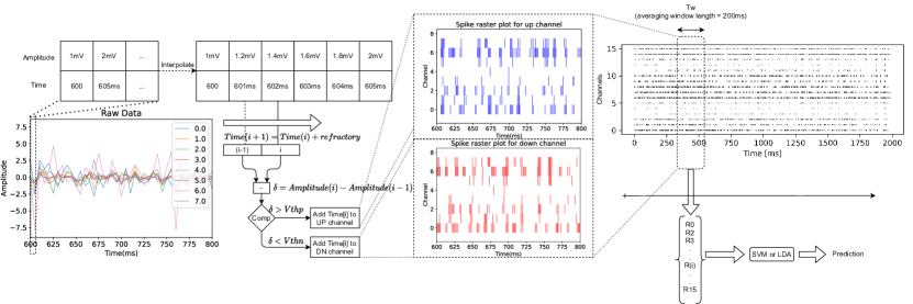
The eight continuous analog EMG signals are encoded as UP and down (DN) spikes. The data is first interpolated and the difference between successive amplitudes is compared to a positive and a negative threshold to obtain spike times. The average firing rate is computed across a time window of 200 ms for each of the 16 spike trains and fed into an SVM classifier.
2.1.1. Encoding
To realize the full potential of event-driven computing, it is essential to perform event-driven sensing. We use the temporal contrast method (Lichtsteiner et al., 2008; Ma et al., 2020; Ceolini et al., [n.d.]) to encode the continuous analog signal to discrete spike trains. In this method, the variation in amplitude is calculated across time. If the difference between a successive sample exceeds a predefined threshold, a spike is generated. We use two separate channels to better represent the signal in a lossless fashion for excitation (positive change in signal amplitude) or depression (negative change in signal amplitude) as shown in Figure 1. For hardware implementation, the successive difference would be calculated with the help of an optimal amplifier topology (Jiménez et al., 2017), and subsequently, this difference would be compared with a predefined threshold with the help of a comparator. This approach’s key parameters are the positive threshold (Vthp), negative threshold (Vthn), interpolation factor, and refractory period. A single analog channel results in two segments of spike times (UP and DN).
2.1.2. Evaluating the encoding algorithm
For solving the classification problem, every algorithm applied to the signal is aimed at extracting information that is valuable for class differentiation. In the literature, the conventional metric used for evaluating the encoding efficiency is the ability to reconstruct the original analog signal and minimize the mean square error (MSE) between the original and reconstructed signals (Petro
et al., 2020). The above is based on the assumption that the entire spectrum of the signal is of interest and any information loss has to be minimized. However, much of the signal component might not be of interest for classification. Tailoring the encoding hyper-parameters to reconstruct the background signal defeats the purpose of event-based sensing. While some studies (Guo
et al., 2021; Anumula
et al., 2018) evaluate the SNN performance to optimize the encoding hyperparameters, the performance is effected by the SNN topology and learning algorithm.
To this end, we propose a novel approach to evaluate and tune our signals to spikes encoding front ends in the context of classification tasks. We refer to as spike encoding & evaluation baseline (spike enc. eval. baseline) (as illustrated in Figure 1). This is, in turn, inspired by the readout method, which is a popular classification strategy for inferring the states of reservoirs. As shown in Figure 1, rate vectors averaged over 200 ms window are classified using a machine learning classifier (linear discriminant analysis (LDA) or support vector machine (SVM)). With help of grid search, the accuracy was computed for different values of positive (0,1) and negative (-1,0) threshold. The selected ones are positive and negative threshold as 0.5 V and -0.5 V respectively.
2.2. Spiking neural network
2.2.1. Recurrent neural networks and Reservoir computing
Recurrent neural networks incorporate the past input memory for computing the output. Recurrent neural networks are thus helpful for processing time-domain signals. Reservoirs inherently behave as recurrent neural networks and are also referred to as Liquid State Machines (LSM) (Maass et al., 2002) and Echo State Networks (ESN) (Jaeger, 2001). An efficient reservoir projects the input signal into a space of linearly separable vectors so that the decision can be computed by processing the network state (e.g. firing rate) through simple machine learning classifiers. Inferring from the reservoir of neurons consists of feeding in a signal of interest and matching the reservoir neurons’ time-series signals to a training signal related to the input signal of the same class (Carroll, 2019).
2.2.2. Neuron
Neurons perform temporal and spatial integration of weighted spikes from the synapses and add non-linearity to the system. Spiking neural networks are composed of neuron models inspired by the biological neuron. Leaky integrate and fire (LIF) neuron (Abbott, 1999) is a good balance between biological plausibility and computational feasibility and hence used in this study. A key feature of a biological neuron is homeostasis or adaptation; when a neuron is stimulated repeatedly, it becomes less sensitive to the stimulation, and the firing rate decreases. To account for homeostasis, we implement adaptive LIF neurons (Brodeur and Rouat, 2012).
The neuron integrates the incoming signal, with leakage (time constant of to resting membrane voltage of ), which is described by
| (1) |
When the neuron membrane potential () reaches a threshold level (), a spike is generated and the neuron membrane potential resets to the reset voltage (). After each spike, the threshold is incremented by an adaptive threshold increment value (), which in turn also leaks (to with time constant of ) to decrease the threshold in the absence of stimulation which is described by
| (2) |
| (3) |
The parameters along with descriptions are tabulated in Table 1.

EMG processing pipeline and reservoir topology
| Parameter | Value | Description | ||
| v0 | 0 V |
|
||
| 15 to 25 ms | Leak time constant | |||
| refractory | 1 ms | Refractory period | ||
| 1 V |
|
|||
| 100 mV |
|
|||
| 50 ms |
|
2.2.3. Synapses and activity regulation
The synaptic transmission is based on equation (4). The weights are initialized in the range [0, 0.25] with uniform distribution. Plasticity is implemented in ’w’ governed by the CRITICAL learning rule (Brodeur and Rouat, 2012) which maximizes the reservoir’s sensitivity.
| (4) |
| Parameter | Value | ||
| Shape of macrocolumn | [2,5,1] | ||
| Shape of minicolumn | [4,4,2] | ||
| Connectivity | Small world | ||
| Size of reservoir population | 320 | ||
|
0.8 | ||
|
1161 | ||
| Number of input connections | 174 | ||
| Initial input weights | 0 to 1 | ||
| Initial reservoir weights | 0 to 0.25 | ||
|
0.1 | ||
|
1 | ||
|
CRITICAL |
Reservoirs are prone to various problems in the balance of the spike activity. Either too much or too little activity is not effective in maintaining a working memory inside the reservoir, which is crucial for their implementation. The ”edge-of-chaos,” or criticality, has been shown to be an adequate target for reaching this balance. In order to maintain this balance, an adaptation mechanism must be implemented inside the reservoir. For this purpose, the CRITICAL learning rule (Brodeur and Rouat, 2012) was chosen as a local weight regulation plasticity rule. The usage of CRITICAL should allow the weights of the reservoir to be in a more desirable state than fully random initialization. The CRITICAL learning rule tunes the weights such that the local branching factor of every neuron reaches a target value. It is believed that maintaining the local branching factor near one will keep the reservoir at this ”edge-of-chaos” (Haldeman and Beggs, 2005). A branching factor of 1 conceptually means that a spike generated by any reservoir neuron would lead to, on average, a single spike in all of the postsynaptic neurons.
2.2.4. Topology
It is important to note that CRITICAL does not influence the reservoir’s connectivity, but only the weights. Therefore, the network connectivity must still be chosen adequately. For this purpose, the initial connectivity of the reservoir is a small-world-like topology (Wijesinghe et al., 2019; Davey et al., 2006) with the same parameters that were optimized with biologically realistic spectral values in (Balafrej and Rouat, 2020). The neurons are arranged in tri-dimensional minicolumns, as shown in Figure 3, and the probability of connection between two random neurons is purely euclidean distance-based. As an example, in Figure 3, there is 8 minicolumns in the macrocolumnar organization, with each having 32 neurons for a total of 256 neurons inside the reservoir. The connections between the input neurons and the reservoir neurons are made randomly, with the total number of input connections being 15% of reservoir connections (Brodeur and Rouat, 2012). The input connection density was optimized for performance. Lastly, all of the reservoir neurons are read when feeding the classifier.
All parameters for a reservoir of 320 neurons are listed in Table 2. The number of neuron were chosen to 320 in order to benchmark the results with respect to the ones reported in (Ma et al., 2020, [n.d.]). The simulations were performed with time step, dt = 1 ms and using Brian2 (Stimberg et al., 2019) simulator.
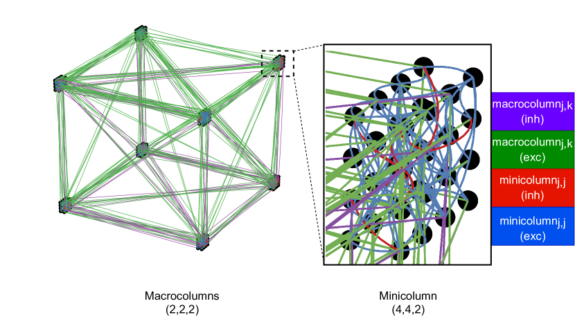
Small world topology for the reservoir of macrocolumn shape : [2,2,2], minicolumn shape of [4,4,2], and 256 neurons. The excitatory and inhibitory connections between neurons from the same minicolumn and across macro columns are shown in the legend’s lines of color.
2.3. Readout
The state of the reservoir is extracted in the form of each neuron’s mean firing rate across a time duration of 200 ms. The readout layer is inherently memoryless, as its value is not dependent upon a signal from the past. The resultant rate vector is fed into a classical machine learning classifier, which is a support vector machine with a radial basis function kernel (Boser et al., 1992) in this study. The regularization parameter (C) was chosen to be 1 while the parameter kernel coefficient (Gamma) was chosen to be 1/(number of features), note the number of features is equal to 16 for spike encoding baseline and number of reservoir neurons for reservoir computing.
| Dataset | Method |
|
Accuracy () | ||
|---|---|---|---|---|---|
| Roshambo | Spike Enc. & Eval. Baseline | LDA | 74.61 2.44% | ||
| SVM | 85.44 0.75% | ||||
| Reservoir (No plasticity) | LDA | 76.44 1.80% | |||
| SVM | 81.83 0.93% | ||||
| Reservoir (CRITICAL) | LDA | 83.06 0.92% | |||
| SVM | 88.00 0.29% | ||||
| Sensor fusion (EMG) | Spike Enc. & Eval. Baseline | LDA | 53.03 1.38% | ||
| SVM | 65.18 3.28% | ||||
| Reservoir (No plasticity) | LDA | 55.97 2.07% | |||
| SVM | 62.33 2.05% | ||||
| Reservoir (CRITICAL) | LDA | 61.96 2.99% | |||
| SVM | 70.60 3.65% |
3. Results and Discussions
We propose two pipelines, the Spike Encoding & Evaluation Baseline as presented in Figure 1, and an encoder followed by a CRITICAL-enabled reservoir as shown in Figure 2. Rather than minimizing the error in signal reconstruction, we optimize the encoding parameters by maximizing the accuracy of a supervised readout layer trained with the average rate vectors as shown in Figure 1. Data from 1 session was taken for testing from the three sessions, and the other two were used for training the machine learning classifier. The three-fold classification accuracy for two machine learning classifiers : LDA and SVM (RBF kernel) are reported in Table 3. We observe a higher accuracy for the SVM classifier than the LDA classifier and hence use that for comparing performance with literature (Table 4).
With the Spike Encoder & Evaluation Baseline we obtained 85.44% accuracy using the Roshambo dataset and 65.18% for the EMG subset of sensor fusion dataset. The classification performance for this method was found to be higher than the ones reported in the literature by using reservoirs with fixed weights in the case of the Roshambo dataset and by using spiking multilayer perceptron (MLP) and spiking convolutional neural network (CNN) for the sensor fusion dataset. This illustrates the high performance of event-based sensing of electrophysiological signals and low power budget and transmission bandwidth requirement. The Spike Encoding & Evaluation Baseline seems to be an excellent reference to which novel neuromorphic SNN classifiers can be compared.
| Dataset | Ref | Method | Accuracy | ||
| Roshambo | (Ma et al., 2020) |
|
73.2 % | ||
|
77.0 0.5% | ||||
|
60.0 1.4% | ||||
| (Ma et al., [n.d.]) |
|
85.28% | |||
|
75% | ||||
| This work |
|
85.44 0.75% | |||
|
88.00 0.29% | ||||
| Sensor fusion (EMG) | (Ceolini et al., [n.d.]) | MLP | 67.2 3.6% | ||
| CNN | 68.1 2.8% | ||||
| Spiking MLP | 53.6 1.4% | ||||
| Spiking CNN | 55.7 2.7% | ||||
| This work |
|
65.07 3.2% | |||
|
70.60 3.65% |
The architecture shown in Figure 2 uses a spiking reservoir with bio-inspired topology from (Balafrej and Rouat, 2020) for features extraction. With plasticity in the reservoir performance improves further. We implemented the CRITICAL auto-regulation synaptic plasticity in synapses emerging from excitatory neurons. The classification performance for both datasets is reported in Table 3, and compared in Table 4 with state of the art systems. The reservoir’s performance are compared between fixed weights and with that of a reservoir with CRITICAL plasticity.
Interestingly, the reservoir’s performance with fixed weights was lower than that of the Spike Encoding & Evaluation Baseline with SVM readout for both datasets, indicating information loss in the reservoir’s activity, possibly due to chaos. This highlights the importance of using a reference system like our proposed Spike Encoding & Evaluation Baseline to challenge neural architectures. Moreover, the LDA classifier’s performance was higher for the fixed weight reservoir than the Spike Encoding & Evaluation Baseline, which validates the proposition that a reservoir projects the signals to a linearly separable hyper-dimensional vector space.
The reservoir performance with regulated activity was found to be more than 88% (320 reservoir neurons) for the Roshambo dataset and 70.6% (2048 reservoir neurons) for the sensor fusion dataset. Importantly, the performance figure is higher than fixed weight reservoir (Ma et al., 2020, [n.d.]) for the Roshambo dataset, and the state-of-the-art CNN (Ceolini et al., [n.d.]) for sensor fusion dataset as shown in Table 4. Hence, the initial hypothesis of the reservoir’s increased performance at the edge of chaos is corroborated.
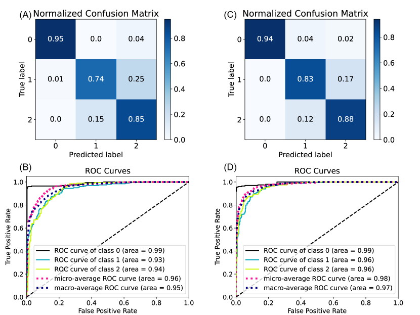
Roshambo dataset, where class 0,1,2 are ’rock’, ’paper’, and ’scissor’. (A) and (B) are the confusion matrix and ROC curve for the Spike Encoding & Evaluation Baseline, (C) and (D) are confusion matrix and ROC curve of the reservoir of 320 neurons, CRITICAL plasticity, and SVM based readout
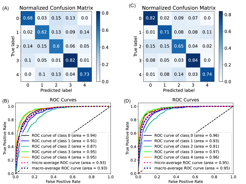
The confusion matrix and receiver operating characteristic (ROC) curve for the Spike Encoding & Evaluation Baseline are shown in Figures 4(A) and 4(B) for the Roshambo dataset. The ROC curves are used to study the tradeoff between specificity (1 - false-positive rate) and sensitivity (true positive rate), with a classifier closer to the top left indicating better performance and area under curve (AOC) equal to one. AOC score is computed for each class and averaged irrespective of individual class size for computing the macro-average of the AOC. For computing the micro-average, the averaging is weighted by class size. The micro-average and macro-ave rage of the AOC are almost identical indicating class balance and uniform performance across dataset. The recognition for the correct class reaches up to 98% in the case of a regulated reservoir-based approach. Lower accuracy is seen for differentiating movement with similar muscle pathways, i.e., paper and scissor. The confusion matrix and ROC curve for SVM readout performed on encoded data are shown in Figures 5(A) and 5(B) for the sensor fusion dataset. The accuracy for the correct class reaches up to 80%. Designing a system with commands associated with a similar muscle pathway, or low accuracy of differentiability should be avoided.
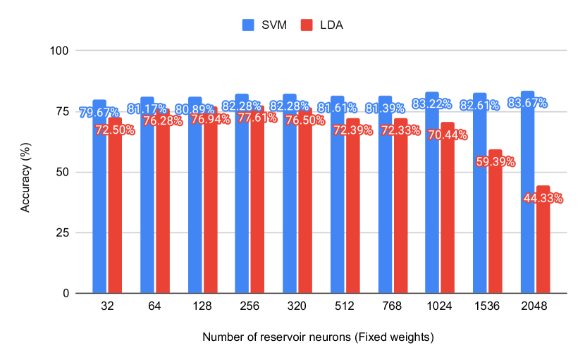
Classification accuracy for the Roshambo dataset plotted against the number of reservoir neurons. The CRITICAL learning rule is implemented in recurrent connections, and SVM or LDA is used in the readout layer.
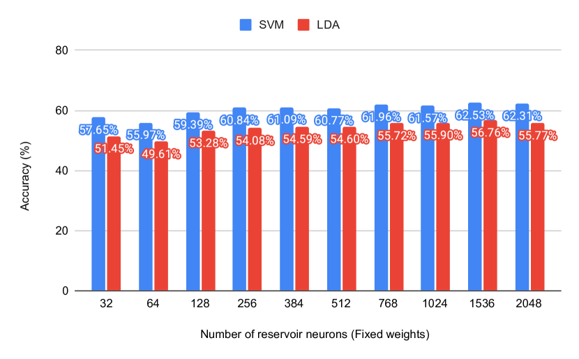
Classification accuracy for sensor fusion dataset (5 class) plotted against the number of reservoir neurons. The CRITICAL learning rule is implemented in recurrent connections, and SVM or LDA is used in the readout layer.
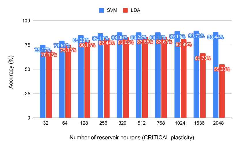 \DescriptionClassification accuracy for the Roshambo dataset plotted against the number of reservoir neurons. The CRITICAL learning rule is implemented in recurrent connections, and SVM or LDA is used in the readout layer.
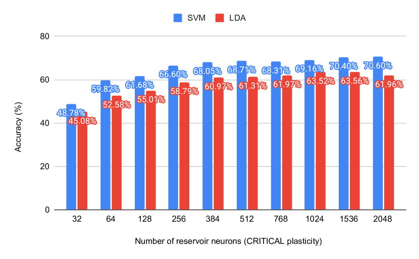 \DescriptionClassification accuracy for sensor fusion dataset (5 class) plotted against the number of reservoir neurons. The CRITICAL learning rule is implemented in recurrent connections, and SVM or LDA is used in the readout layer.
The classification performance was plotted against the number of neurons for reservoir with fixed weights and regulated reservoir in Figures 9 and 9 and Figures 9 and 9 for Roshambo and sensor fusion dataset, respectively. The classification performance increases with the number of neurons consistently for the sensor fusion dataset with the SVM-based reservoir’s readout. For the Roshambo dataset, the best performance of 89.72 % was observed for 1536 neurons and activity regulation. This highlights the importance of selecting the size of reservoir for complexity of task (number of classes), and size of dataset. A degradation of performance was observed for the LDA classifier while increasing the number of neurons beyond a limit. This highlights the limitation of the simple readout classifier, and need for a more sophisticated classifier like SVMs.
4. Conclusion and future scope
Sensing and processing electrophysiological data is one of the key applications of AI deployment on edge devices. Spike encoding is an important step in the neuromorphic computing pipeline, and it is crucial to ensure that important information for classification is preserved. It is also important to evaluate the efficiency of encoding before passing the information to a SNN to establish a baseline for comparing different SNN topologies and plasticity mechanisms. The high performance of the simple machine learning classifier (Spike Encoding & Evaluation Baseline) applied to raw spike converted data in the absence of any signal processing, and the feature extraction method validates the proposition of using event-based sensors to measure biopotential signals. The regulated reservoir of spiking neurons operating with a branching factor of one performs better than the state-of-the-art CNN (Ceolini et al., [n.d.]), which further validates reservoir computing’s applicability for processing time-series data when operating at the edge of chaos. The reservoir performance with regulated activity reached up to 89.72% for the Roshambo EMG dataset (Donati, 2019) and 70.6% for the EMG subset of sensor fusion dataset (Ceolini et al., 2020).
In a real-world deployment, essentially, a null class should also be present to avoid the actuator command in the resting state. As the availability of open-source data is limited, such a system could not be trained and evaluated in this study. In the future, we plan to incorporate more gestures along with the resting-state class. Finally, the readout layer, although efficient, is not biologically plausible. In the future, we will explore more biologically plausible readout classifiers in the context of life-long learning.
5. Author Contributions
J.R., Y.B., F.A., and D.D. contributed in formulating the study. N.G. designed and performed the experiments and derived the models. N.G., I.B., F.A., and Y.B. analysed the data. N.G. took the lead in writing the manuscript. All authors provided critical feedback and helped shape the research, analysis and manuscript.
Acknowledgements.
We acknowledge financial supports from the EU: ERC-2017-COG project IONOS (# GA 773228) and CHIST-ERA UNICO project. This work was also supported by Natural Sciences and Engineering Research Council of Canada (NSERC) and Fond de Recherche du Québec Nature et Technologies (FRQNT).References
- (1)
- Abbott (1999) L. Abbott. 1999. Lapicque’s introduction of the integrate-and-fire model neuron (1907). Brain Research Bulletin 50 (1999), 303–304.
- Anumula et al. (2018) J. Anumula, D. Neil, T. Delbruck, and S. C. Liu. 2018. Feature Representations for Neuromorphic Audio Spike Streams. Frontiers in Neuroscience 12 (feb 2018). https://doi.org/10.3389/fnins.2018.00023
- Balafrej and Rouat (2020) I. Balafrej and J. Rouat. 2020. P-CRITICAL: A Reservoir Autoregulation Plasticity Rule for Neuromorphic Hardware. ArXiv abs/2009.05593 (2020).
- Boser et al. (1992) B. E. Boser, I. M. Guyon, and V. N. Vapnik. 1992. A training algorithm for optimal margin classifiers. In Proceedings of the fifth annual workshop on Computational learning theory - COLT '92. ACM Press. https://doi.org/10.1145/130385.130401
- Boström et al. (2013) K. Boström, H. Wagner, M. Prieske, and M. D. de Lussanet. 2013. Model for a flexible motor memory based on a self-active recurrent neural network. Human movement science 32 5 (2013), 880–98.
- Brodeur and Rouat (2012) S. Brodeur and J. Rouat. 2012. Regulation toward Self-organized Criticality in a Recurrent Spiking Neural Reservoir. In Artificial Neural Networks and Machine Learning – ICANN 2012, Alessandro E. P. Villa, Włodzisław Duch, Péter Érdi, Francesco Masulli, and Günther Palm (Eds.). Springer Berlin Heidelberg, Berlin, Heidelberg, 547–554.
- Carroll (2019) T. Carroll. 2019. Mutual Information and the Edge of Chaos in Reservoir Computers. ArXiv abs/1906.03186 (2019).
- Ceolini et al. ([n.d.]) E. Ceolini, C. Frenkel, S. B. Shrestha, G. Taverni, L. Khacef, M. Payvand, and E. Donati. [n.d.]. Hand-Gesture Recognition Based on EMG and Event-Based Camera Sensor Fusion: A Benchmark in Neuromorphic Computing. ([n. d.]).
- Ceolini et al. (2020) E. Ceolini, G. Taverni, M. Payvand, and E. Donati. 2020. EMG and Video Dataset for sensor fusion based hand gestures recognition. https://doi.org/10.5281/zenodo.3663616
- Chen et al. (2006) D. Chen, Y. Li, Dongming Xu, J. Harris, and J. Príncipe. 2006. Asynchronous biphasic pulse signal coding and its CMOS realization. 2006 IEEE International Symposium on Circuits and Systems (2006), 4 pp.–2296.
- Cordella et al. (2016) F. Cordella, A. Ciancio, R. Sacchetti, A. Davalli, A. Cutti, E. Guglielmelli, and L. Zollo. 2016. Literature review on needs of upper limb prosthesis users. Frontiers in neuroscience 10 (2016), 209.
- Corradi and Indiveri (2015) F. Corradi and G. Indiveri. 2015. A Neuromorphic Event-Based Neural Recording System for Smart Brain-Machine-Interfaces. IEEE Transactions on Biomedical Circuits and Systems 9, 5 (2015), 699–709.
- Davey et al. (2006) N. Davey, L. Calcraft, and R. Adams. 2006. High capacity, small world associative memory models. Connection Science 18 (2006), 247 – 264.
- Donati (2019) E. Donati. 2019. EMG from forearm datasets for hand gestures recognition. https://doi.org/10.5281/zenodo.3194792
- Donati et al. (2019) E. Donati, M. Payvand, N. Risi, R. Krause, and G. Indiveri. 2019. Discrimination of EMG Signals Using a Neuromorphic Implementation of a Spiking Neural Network. IEEE Transactions on Biomedical Circuits and Systems 13, 5 (2019), 795–803. https://doi.org/10.1109/TBCAS.2019.2925454
- Guo et al. (2021) W. Guo, M. Fouda, A. Eltawil, and K. N. Salama. 2021. Neural Coding in Spiking Neural Networks: A Comparative Study for Robust Neuromorphic Systems. Frontiers in Neuroscience 15 (2021).
- Haldeman and Beggs (2005) Clayton Haldeman and John M Beggs. 2005. Critical branching captures activity in living neural networks and maximizes the number of metastable states. Phys. Rev. Lett. 94, 5 (2005), 1–4. https://doi.org/10.1103/PhysRevLett.94.058101
- Jaeger (2001) H. Jaeger. 2001. The ”echo state” approach to analysing and training recurrent neural networks.
- Jiménez et al. (2017) J. Jiménez, Shanshan Dai, and J. Rosenstein. 2017. A microwatt front end and asynchronous ADC for sparse biopotential acquisition. 2017 IEEE 60th International Midwest Symposium on Circuits and Systems (MWSCAS) (2017), 503–506.
- Kannenberg (2017) A. Kannenberg. 2017. Active Upper-Limb Prostheses: The International Perspective. Journal of Prosthetics and Orthotics 29 (2017), P57–P62.
- Legenstein and Maass (2007) R. Legenstein and W. Maass. 2007. Edge of chaos and prediction of computational performance for neural circuit models. Neural networks : the official journal of the International Neural Network Society 20 3 (2007), 323–34.
- Lichtsteiner et al. (2008) P. Lichtsteiner, C. Posch, and T. Delbruck. 2008. A 128 128 120 dB 15 s Latency Asynchronous Temporal Contrast Vision Sensor. IEEE Journal of Solid-State Circuits 43, 2 (2008), 566–576.
- Lusardi et al. (2013) M. Lusardi, M. Jorge, and C. Nielsen. 2013. Orthotics and Prosthetics in Rehabilitation-E-Book. Elsevier Health Sciences.
- Ma et al. ([n.d.]) Y. Ma, B. Chen, P. Ren, N. Zheng, G. Indiveri, and E. Donati. [n.d.]. EMG-Based Gestures Classification Using a Mixed-Signal Neuromorphic Processing System. IEEE Journal on Emerging and Selected Topics in Circuits and Systems ([n. d.]).
- Ma et al. (2020) Y. Ma, E. Donati, B. Chen, P. Ren, N. Zheng, and G. Indiveri. 2020. Neuromorphic Implementation of a Recurrent Neural Network for EMG Classification. In 2020 2nd IEEE International Conference on Artificial Intelligence Circuits and Systems (AICAS). 69–73.
- Maass et al. (2002) W. Maass, T. Natschläger, and H. Markram. 2002. Real-Time Computing Without Stable States: A New Framework for Neural Computation Based on Perturbations. Neural Computation 14 (2002), 2531–2560.
- Mead (2020) C. Mead. 2020. How we created neuromorphic engineering. Nature Electronics 3 (07 2020), 434–435. https://doi.org/10.1038/s41928-020-0448-2
- Moinnereau et al. (2018) M. Moinnereau, T. Brienne, S. Brodeur, J. Rouat, K. Whittingstall, and E. Plourde. 2018. Classification of auditory stimuli from EEG signals with a regulated recurrent neural network reservoir. ArXiv abs/1804.10322 (2018).
- Peng et al. (2015) L. Peng, Z. Hou, N. Kasabov, G. Bian, L. Vladareanu, and H. Yu. 2015. Feasibility of NeuCube spiking neural network architecture for EMG pattern recognition. In 2015 International Conference on Advanced Mechatronic Systems (ICAMechS). 365–369. https://doi.org/10.1109/ICAMechS.2015.7287090
- Petro et al. (2020) B. Petro, N. Kasabov, and R. M. Kiss. 2020. Selection and Optimization of Temporal Spike Encoding Methods for Spiking Neural Networks. IEEE Transactions on Neural Networks and Learning Systems 31, 2 (2020), 358–370.
- Phinyomark et al. (2011) A. Phinyomark, P. Phukpattaranont, and C. Limsakul. 2011. A Review of Control Methods for Electric Power Wheelchairs Based on Electromyography Signals with Special Emphasis on Pattern Recognition. IETE Technical Review 28 (2011), 316 – 326.
- Phinyomark and Scheme (2018) A. Phinyomark and E. Scheme. 2018. EMG Pattern Recognition in the Era of Big Data and Deep Learning. Big Data and Cognitive Computing 2, 3 (aug 2018), 21. https://doi.org/10.3390/bdcc2030021
- Scheme and Englehart (2011) E. Scheme and K. Englehart. 2011. Electromyogram pattern recognition for control of powered upper-limb prostheses: state of the art and challenges for clinical use. Journal of rehabilitation research and development 48 6 (2011), 643–59.
- Spiewak (2018) C. Spiewak. 2018. A Comprehensive Study on EMG Feature Extraction and Classifiers. Open Access Journal of Biomedical Engineering and Biosciences 1, 1 (feb 2018). https://doi.org/10.32474/oajbeb.2018.01.000104
- Stimberg et al. (2019) M. Stimberg, R. Brette, and D. F. Goodman. 2019. Brian 2, an intuitive and efficient neural simulator. eLife 8 (Aug. 2019), e47314. https://doi.org/10.7554/eLife.47314
- Wen and Boahen (2009) B. Wen and K. Boahen. 2009. A Silicon Cochlea With Active Coupling. IEEE Transactions on Biomedical Circuits and Systems 3, 6 (2009), 444–455. https://doi.org/10.1109/TBCAS.2009.2027127
- Wijesinghe et al. (2019) P. Wijesinghe, G. Srinivasan, P. Panda, and K. Roy. 2019. Analysis of Liquid Ensembles for Enhancing the Performance and Accuracy of Liquid State Machines. Frontiers in Neuroscience 13 (2019), 504. https://doi.org/10.3389/fnins.2019.00504